RRID:CVCL_7254
DOI: 10.1038/s41420-026-02945-y
Resource: (KCLB Cat# 80009, RRID:CVCL_7254)
Curator: @scibot
SciCrunch record: RRID:CVCL_7254
RRID:CVCL_7254
DOI: 10.1038/s41420-026-02945-y
Resource: (KCLB Cat# 80009, RRID:CVCL_7254)
Curator: @scibot
SciCrunch record: RRID:CVCL_7254
RRID:AB_2863407
DOI: 10.1038/s41420-026-02945-y
Resource: (ABclonal Cat# A4992, RRID:AB_2863407)
Curator: @scibot
SciCrunch record: RRID:AB_2863407
RRID:AB_2194997
DOI: 10.1038/s41420-026-02945-y
Resource: (Santa Cruz Biotechnology Cat# sc-21742, RRID:AB_2194997)
Curator: @scibot
SciCrunch record: RRID:AB_2194997
RRID:CVCL_0546
DOI: 10.1038/s41420-026-02945-y
Resource: (KCB Cat# KCB 200848YJ, RRID:CVCL_0546)
Curator: @scibot
SciCrunch record: RRID:CVCL_0546
RRID:CVCL_B288
DOI: 10.1038/s41420-026-02945-y
Resource: (RRID:CVCL_B288)
Curator: @scibot
SciCrunch record: RRID:CVCL_B288
RRID:AB_3675962
DOI: 10.1038/s41420-026-02945-y
Resource: None
Curator: @scibot
SciCrunch record: RRID:AB_3675962
RRID:AB_3675929
DOI: 10.1038/s41420-026-02945-y
Resource: None
Curator: @scibot
SciCrunch record: RRID:AB_3675929
RRID:AB_228307
DOI: 10.1007/s12035-026-05709-y
Resource: (Thermo Fisher Scientific Cat# 31430, RRID:AB_228307)
Curator: @scibot
SciCrunch record: RRID:AB_228307
RRID:AB_2892717
DOI: 10.1007/s12035-026-05709-y
Resource: (Abcam Cat# ab218624, RRID:AB_2892717)
Curator: @scibot
SciCrunch record: RRID:AB_2892717
RRID:AB_887691
DOI: 10.1007/s12035-026-05709-y
Resource: (Synaptic Systems Cat# 155 003, RRID:AB_887691)
Curator: @scibot
SciCrunch record: RRID:AB_887691
RRID:AB_11211734
DOI: 10.1007/s12035-026-05709-y
Resource: (Millipore Cat# AB9884, RRID:AB_11211734)
Curator: @scibot
SciCrunch record: RRID:AB_11211734
RRID:AB_476693
DOI: 10.1007/s12035-026-05709-y
Resource: (Sigma-Aldrich Cat# A2066, RRID:AB_476693)
Curator: @scibot
SciCrunch record: RRID:AB_476693
RRID:AB_2566521
DOI: 10.1007/s12035-026-05709-y
Resource: (BioLegend Cat# 836304, RRID:AB_2566521)
Curator: @scibot
SciCrunch record: RRID:AB_2566521
RRID:AB_10691711
DOI: 10.1007/s00018-026-06092-6
Resource: (Cell Signaling Technology Cat# 5153, RRID:AB_10691711)
Curator: @scibot
SciCrunch record: RRID:AB_10691711
In 1731, Manuel Trujillo accused two Pueblo men, Acensio Povia and Antonio Yuba, of committing sodomy. Both Povia and Yuba denied this accusation, and Yuba invoked his status as a Christian in order to bolster his credibility. Governor Gervasio Cruzat y Góngora chose to exile Povia and Yuba to different pueblos for a period of four months, during which time they were to cease any and all communication with one another. This case explores sexual practices deemed “nefarious sins” as well as illustrates what scholars have called the colonial dilemma—the situation where Indigenous peoples remained in a subjected state despite theological equality following their Christian conversion
The Faith and law aspect backing the rest of civilization was a moral inspiration to the culture to come, not an invitation for those already deemed savages (indigenous) for the unfair treatment they'd received being natives, as ultimately contradicting freedom implied by the ownership of the land and its governing. Laws against sexual promiscuity becoming the for front of laws is always related to the assimilation of nationals vs. dominants.
The four “spanned all the different areas of expertise
La interdisciplinaridad esta presente en cada área del conocimiento, lo que me hacer pensar en lo incorrecto de afirmar que desde nuestra carrera de ciencia de la información solo tenemos los campos de acción de la biblioteca y del archivo, cuando en realidad podemos desenvolvernos en distintos sectores para lograr un objetivo en común, como es el caso de este programa.
Tus artículos y mensajes de estado pueden transmitirse a todos los servicios, no solamente uno,
Según lo que pude leer y entender, se usa el modelo POSSE, para que los demás puedan leer lo que uno publica sin importar el sitio, lo que realmente me parece útil debido a que es una solución directa a esa costumbre de sitios a obligarnos a que creemos cuentas para la interacción.
Puedes publicar lo que quieras, en el formato que quieras, sin que nadie te monitoree. Adicionalmente, compartes enlaces permanentes, que siempre funcionarán, bien sean simples y legibles en tu propio dominio (como ejemplo.com/ideas) o cipherlinks, que funcionan incluso si no tienes un dominio, este cambia o está caído/inaccesible.
Este sitio web es muy similar Hypothesis, es una herramienta de anotación colaborativa que permite que la lectura sea activa, visible y social; sin que tenga ninguna restricción, que permite tener el control y responsabilidad de lo que publica.
Brea es un generador y gestor de sitios web enfocado en la personalización interactiva y la autonomía,
Cuando se menciona algún generador de sitios web automáticamente pienso en plataformas como Wix donde se puede hacer una gestión de contenidos de manera sencilla aunque dependa de una suscripción, por lo que una propuesta de este tipo combinando las dinámicas de generación de sitios web y un CMS me parece una forma más libre de interactuar con estas páginas al mencionar a tecnologías como Fossil ya que es una alternativa a Git.
Al tener más en detalle que es un CMS y un Generador de Sitios Web Estáticos siendo buenos ejemplos wikis o plataformas que usan Markdown es muy interesante ese puente entre dos plataformas que se conforman a partir de la interacción entre usuarios y la colaboración entre ellos dando a relucir el trabajo colaborativo de una manera más fácil y cercana
Brea es un generador y gestor de sitios web enfocado en la personalización interactiva y la autonomía, que permite publicar información integrada desde distintas fuentes, con presentaciones a la medida. Está a medio camino entre un generador de sitios web estáticos y un Sistema Gestor Contenidos (o CMS) desacoplado, debido a la combinación de tecnologías como Fossil y Pharo, que permiten una eficiente gestión, replicación y publicación de archivos estáticos y un entorno de programación en vivo (live coding), para extender y manipular las fuentes de datos, sus presentaciones e interfaces.
nos muestra con claridad la identidad "híbrida" de Brea, ya que nos dice cómo se posiciona a Brea no solo como una herramienta de publicación al estar entre un sitio estático y un CMS, resuelve el gran dilema de las webs actuales.
Flexibilidad : Al integrar Fossil, rompe la normatividad de los sistemas cerrados, el uso de "live coding" permite que el usuario no solo llene "cajitas de texto"
Tus datos y contenido son tuyos Cuando publicas algo en la web, debería pertenecerte a ti, no a una empresa. Demasiadas compañías han cerrado y perdido todos los datos de sus usuarios. Otras tienen algoritmos opacos que mercantilizan tu privacidad y condicionan tus hábitos, bajo lógicas extractivistas. Uniéndote a la IndieWeb, tu contenido continúa siendo tuyo y estando bajo tu control.
Lo que quiero resaltar del texto es lo importante de ser dueño de nuestro dominio y nuestros datos, de esta manera garantizamos que nuestra memoria y nuestra creatividad no dependan del permiso de una corporación.
Está a medio camino entre un generador de sitios web estáticos y un Sistema Gestor Contenidos (o CMS) desacoplado, debido a la combinación de tecnologías como Fossil y Pharo,
Considero es una mezcla intermedia entre un lenguaje HTML/JS y un CMS lo cual lo hace un poco mas intuitivo mezclando las mejores partes de cada lado
Interactivas Gracias a Pharo y su entorno de Live Coding, podemos explorar fuentes de datos, construir consultas y ver los cambios al sitio de manera interactiva, agilizando ciclos de realimentación entre creación y creadoras.
En esta era de compartir de manera simultanea, me parece excelente que se creen este tipo de plataformas donde sea ágil y fácil compartir y trabajar sobre un mismo espacio, de esta forma trabajar de manera ágil entre personas de un mismo ámbito y generar grandes resultados esperados si hablamos por ejemplo empresarialmente.
Cuando publicas algo en la web, debería pertenecerte a ti, no a una empresa.
Me parece muy adecuado el hecho de que en verdad nos pertenece lo que hagamos, pues en paginas como wix, por más que uno pague por el tu dominio y tal, todo esta almacenado en los servidores de ellos, si ellos cierran todo se va, mientras que aca se especifica que me pertenece ese aspecto
permite publicar información integrada desde distintas fuentes
Este apartado, puede relacionarse con los procesos pertenecientes a la Ciencia de la Información, ya que para la integración de información de diferentes fuentes, es necesario hacer la selección, normalización y organización de la información, lo que favorece a la experiencia del usuario final en IndieWeb.
Cuando publicas algo en la web, debería pertenecerte a ti, no a una empresa.
Esta idea en particular es la misma que pudimos observar en el video de Hypothesis, una web libre en donde nuestras acciones no están restringidas por las normativas o reglas de una empresa, y que hemos visto en clase, mediante las alternativas al monopolio de los gigantes tecnológicos como Google y su navegador
uando publicas algo en la web, debería pertenecerte a ti, no a una empresa. Demasiadas compañías han cerrado y perdido todos los datos de sus usuarios. Otras tienen algoritmos opacos que mercantilizan tu privacidad y condicionan tus hábitos, bajo lógicas extractivistas. Uniéndote a la IndieWeb, tu contenido continúa siendo tuyo y estando bajo tu control.
Esto es algo valioso, ya que en esta era de la información desbordada, cualquier cosa que hagamos en la red queda guardada, llega un punto donde en los navegadores que hemos usado aparecen productos o servicios que alguna vez buscamos, por eso ahora el chiste es que "Google lee nuestras mentes", pero en realidad es que vigilan todo lo que hacemos y somos un dato monetizable, por consiguiente me parece excelente una web que sea diferente como lo propone esta página.
personalización interactiva y la autonomía,
No es un sitio genérico tipo plantilla rígida, sino que permite personalizar cosas de forma mas dinámica
Está a medio camino entre un generador de sitios web estáticos y un Sistema Gestor Contenidos (o CMS) desacoplado,
Para ver más sobre CMS en la Wikipedia
Information science
La ciencia de la información es una disciplina interdisciplinaria que estudia cómo se produce, organiza, preserva, recupera y utiliza la información para transformar conocimiento y facilitar la toma de decisiones en cualquier ámbito humano. Es decir, no se limita a acumular datos: busca darles sentido, garantizar su accesibilidad y asegurar que circulen de manera ética y útil en la sociedad.
Disciplines and related fields
En pocas palabras, la ciencia de la información ha ido creciendo como un puente que une distintas disciplinas, convirtiéndose en un campo vivo y adaptable, capaz de transformarse según lo que la sociedad y la tecnología van necesitando.
La ciencia de la información, a grandes rasgos, es una disciplina que se encarga de gestionar datos, documentos e información para que no se pierdan y puedan cumplir una función útil, más allá de simplemente almacenarlos, se trata de otorgarles valor y establecer un ciclo que permita organizarlos, analizarlos y utilizarlos con un propósito definido, de este modo, la información deja de verse como algo sin importancia y se transforma en un recurso con poder, que requiere procesos propios para su adecuada gestión y aprovechamiento.
Considero que un gran campo de la Ciencia de la Información esta movido por los avances tecnológicos y como los profesionales en esta área nos adaptamos. esta tecnología. A las técnicos computacionales, la ciencia de datos y la analítica. Eso mezclado con una interacción entre personas y organizaciones las cuales ya tienen un sistema de información.
La ciencia de la información[1][2][3] (abreviada como infosci) es un campo académico que se ocupa principalmente del análisis, recopilación, clasificación, manipulación, almacenamiento, recuperación, movimiento, difusión y protección de la información. [4] Los profesionales dentro y fuera del campo participan en el estudio de la aplicación y uso del conocimiento en las organizaciones. Además, examinan la interacción entre personas, organizaciones y cualquier sistema de información existente. El objetivo de este estudio es crear, reemplazar, mejorar o comprender los sistemas de información.
Para mi la Ciencia de la Información es un campo interdisciplinario que se encarga de analizar cómo se genera, recolecta, organiza, almacena, recupera y transmite la información.
En lugar de centrarse solo en los cables o el código , se enfoca en el vínculo entre las personas y los datos como tal objetivo principal es asegurar que la información sea accesible y útil para quien la necesite.
Es una ciencia interdisciplinaria
Opino que es importante tener en que es una ciencia interdisciplinaria interdisciplinaria porque integra conocimientos y métodos de diversas áreas para comprender, organizar y facilitar el acceso a la información, como las disciplinas que aquí se mencionan
Social media's power to facilitate topics
Las conexiones en redes sociales ayudan a esparcir la información a mayor velocidad, pero es claro que también es un medio de desinformación y nosotros como bibliotecarios debemos saber filtrar dicha información cuando se esparce sin control y dar la información real. Aunque es una tarea difícil este tema debe estar de manera principal para poder solucionar la desinformación.
The discipline of documentation science, which marks the earliest theoretical foundations of modern information science, emerged in the late part of the 19th century in Europe together with several more scientific indexes whose purpose was to organize scholarly literature. Many information science historians cite Paul Otlet and Henri La Fontaine as the fathers of information science with the founding of the International Institute of Bibliography (IIB) in 1895.[31] A second generation of European Documentalists emerged after the Second World War, most notably Suzanne Briet.[32] However, "information science" as a term is not popularly used in academia until sometime in the latter part of the 20th century.[33]
A través de la historia ya habían vestigios de una ciencia para organizar y salvaguardar la información. Solo que no se llamaba como actualmente la conocemos, pero como toda rama comenzó como una necesidad y se fue especializando con el tiempo y dándole forma a lo que actualmente hoy conocemos.
Scope and approach
Somos una carrera que observa todo a su alrededor y comienza a dar mejoras de todo ello según enfoques que sean necesarios, ya sean desarrollos en tecnología o en el ámbito humano, podria decirse que somos un árbol de vida que mantiene cada rama y la nutre.
interdisciplinary
Manteniendo esa línea interdisciplinar y estemos involucrados en todas las áreas del conocimiento, estamos un poco aislados por el poco conocimiento e importancia que nos dan, y mi experiencia dicta que los profesionales a cargo son quienes no saben dar su voz en las instituciones. Y cada nuevo conocimiento y nueva rama que surge nos involucraremos en dicha disciplina.
transdisciplinary field
En este aspecto siento que esta palabra es muy fuerte y muchas personas están llevando estos términos muy allá olvidando los campos ya establecidos y que aun falta por mejorar, cuando uno quiere abarcar todo al tiempo al final no hace nada bien.
Information science
Creo que mas allá del termino lo que significa nuestra carrera, no debemos limitarla a eso, para cada profesional tiene un significado diferente este termino desde las experiencias vividas y desde su labor profesional, para algunos puede ser mas enfocado a lo social y las bibliotecas, para otros mas enfocado a memoria y cultura con el archivo, para otros solo tener un titulo y creerse mas por saber sobre palabras bonitas con significados perfectos. pero en mi humilde opinión la carrera y mas este termino es el sentir de la profesión y como cada uno la aborde desde sus distintos enfoques. Y son igual de validos.
Arguments for Utilitarianismfunction togglePlayOrPause(){document.getElementById("player-container").classList.add("show-player"),document.getElementById("audio-icon").outerHTML=""}Table of ContentsIntroduction: Moral Methodology & Reflective EquilibriumArguments for UtilitarianismWhat Fundamentally MattersThe Veil of IgnoranceEx Ante ParetoExpanding the Moral CircleThe Poverty of the AlternativesThe Paradox of DeontologyThe Hope ObjectionSkepticism About the Distinction Between Doing and AllowingStatus Quo BiasEvolutionary Debunking ArgumentsConclusionResources and Further ReadingIntroduction: Moral Methodology & Reflective EquilibriumYou cannot prove a moral theory. Whatever arguments you come up with, it’s always possible for someone else to reject your premises—if they are willing to accept the costs of doing so. Different theories offer different advantages. This chapter will set out some of the major considerations that plausibly count in favor of utilitarianism. A complete view also needs to consider the costs of utilitarianism (or the advantages of its competitors), which are addressed in Chapter 8: Objections to Utilitarianism. You can then reach an all-things-considered judgment as to which moral theory strikes you as overall best or most plausible.To this end, moral philosophers typically use the methodology of reflective equilibrium. 1 1 This involves balancing two broad kinds of evidence as applied to moral theories:Intuitions about specific cases (thought experiments).General theoretical considerations, including the plausibility of the theory’s principles or systematic claims about what matters.General principles can be challenged by coming up with putative counterexamples, or cases in which they give an intuitively incorrect verdict. In response to such putative counterexamples, we must weigh the force of the case-based intuition against the inherent plausibility of the principle being challenged. This could lead you to either revise the principle to accommodate your intuitions about cases or to reconsider your verdict about the specific case, if you judge the general principle to be better supported (especially if you are able to “explain away” the opposing intuition as resting on some implicit mistake or confusion).As we will see, the arguments in favor of utilitarianism rest overwhelmingly on general theoretical considerations. Challenges to the view can take either form, but many of the most pressing objections involve thought experiments in which utilitarianism is held to yield counterintuitive verdicts.There is no neutral, non-question-begging answer to how one ought to resolve such conflicts. 2 2 It takes judgment, and different people may be disposed to react in different ways depending on their philosophical temperament. As a general rule, those of a temperament that favors systematic theorizing are more likely to be drawn to utilitarianism (and related views), whereas those who hew close to common sense intuitions are less likely to be swayed by its theoretical virtues. Considering the arguments below may thus do more than just illuminate utilitarianism; it may also help you to discern your own philosophical temperament!While our presentation focuses on utilitarianism, it’s worth noting that many of the arguments below could also be taken to support other forms of welfarist consequentialism (just as many of the objections to utilitarianism also apply to these related views). This chapter explores arguments for utilitarianism and closely related views over non-consequentialist approaches to ethics.Arguments for UtilitarianismWhat Fundamentally MattersMoral theories serve to specify what fundamentally matters, and utilitarianism offers a particularly compelling answer to this question.Almost anyone would agree with utilitarianism that suffering is bad, and well-being is good. What could be more obvious? If anything matters morally, human well-being surely does. And it would be arbitrary to limit moral concern to our own species, so we should instead conclude that well-being generally is what matters. That is, we ought to want the lives of sentient beings to go as well as possible (whether that ultimately comes down to maximizing happiness, desire satisfaction, or other welfare goods).Could anything else be more important? Such a suggestion can seem puzzling. Consider: it is (usually) wrong to steal. 3 3 But that is plausibly because stealing tends to be harmful, reducing people’s well-being. 4 4 By contrast, most people are open to redistributive taxation, if it allows governments to provide benefits that reliably raise the overall level of well-being in society. So it’s not that individuals just have a natural right to not be interfered with no matter what. When judging institutional arrangements (such as property and tax law), we recognize that what matters is coming up with arrangements that tend to secure overall good results, and that the most important factor in what makes a result good is that it promotes well-being. 5 5Such reasoning may justify viewing utilitarianism as the default starting point for moral theorizing. 6 6 If someone wants to claim that there is some other moral consideration that can override overall well-being (trumping the importance of saving lives, reducing suffering, and promoting flourishing), they face the challenge of explaining how that could possibly be so. Many common moral rules (like those that prohibit theft, lying, or breaking promises), while not explicitly utilitarian in content, nonetheless have a clear utilitarian rationale. If they did not generally promote well-being—but instead actively harmed people—it’s hard to see what reason we would have to still want people to follow them. To follow and enforce harmful moral rules (such as rules prohibiting same-sex relationships) would seem like a kind of “rule worship”, and not truly ethical at all. 7 7 Since the only moral rules that seem plausible are those that tend to promote well-being, that’s some reason to think that moral rules are, as utilitarianism suggests, purely instrumental to promoting well-being.Similar judgments apply to hypothetical cases in which you somehow know for sure that a typically reliable rule is, in this particular instance, counterproductive. In the extreme case, we all recognize that you ought to lie or break a promise if lives are on the line. In practice, of course, the best way to achieve good results over the long run is to respect commonsense moral rules and virtues while seeking opportunities to help others. (It’s important not to mistake the hypothetical verdicts utilitarianism offers in stylized thought experiments with the practical guidance it offers in real life.) The key point is just that utilitarianism offers a seemingly unbeatable answer to the question of what fundamentally matters: protecting and promoting the interests of all sentient beings to make the world as good as it can be.The Veil of IgnoranceHumans are masters of self-deception and motivated reasoning. If something benefits us personally, it’s all too easy to convince ourselves that it must be okay. We are also more easily swayed by the interests of more salient or sympathetic individuals (favoring puppies over pigs, for example). To correct for such biases, it can be helpful to force impartiality by imagining that you are looking down on the world from behind a “veil of ignorance”. This veil reveals the facts about each individual’s circumstances in society—their income, happiness level, preferences, etc.—and the effects that each choice would have on each person, while hiding from you the knowledge of which of these individuals you are. 8 8 To more fairly determine what ideally ought to be done, we may ask what everyone would have most personal reason to prefer from behind this veil of ignorance. If you’re equally likely to end up being anyone in the world, it would seem prudent to maximize overall well-being, just as utilitarianism prescribes. 9 9How much weight we should give to the verdicts that would be chosen, on self-interested grounds, from behind the veil? The veil thought experiment highlights how utilitarianism gives equal weight to everyone’s interests, without bias. That is, utilitarianism is just what we get when we are beneficent to all: extending to everyone the kind of careful concern that prudent people have for their own interests. 10 10 But it may seem question-begging to those who reject welfarism, and so deny that interests are all that matter. For example, the veil thought experiment clearly doesn’t speak to whether non-sentient life or natural beauty has intrinsic value. It’s restricted to that sub-domain of morality that concerns what we owe to each other, where this includes just those individuals over whom our veil-induced uncertainty about our identity extends: presently existing sentient beings, perhaps. 11 11 Accordingly, any verdicts reached via the veil of ignorance will still need to be weighed against what we might yet owe to any excluded others (such as future generations, or non-welfarist values).Still, in many contexts other factors will not be relevant, and the question of what we morally ought to do will reduce to the question of how we should treat each other. Many of the deepest disagreements between utilitarians and their critics concern precisely this question. And the veil of ignorance seems relevant here. The fact that some action is what everyone affected would personally prefer from behind the veil of ignorance seems to undermine critics’ claims that any individual has been mistreated by, or has grounds to complain about, that action.Ex Ante ParetoA Pareto improvement is better for some people, and worse for none. When outcomes are uncertain, we may instead assess the prospect associated with an action—the range of possible outcomes, weighted by their probabilities. A prospect can be assessed as better for you when it offers you greater well-being in expectation, or ex ante. 12 12 Putting these concepts together, we may formulate the following principle:Ex ante Pareto: in a choice between two prospects, one is morally preferable to another if it offers a better prospect for some individuals and a worse prospect for none.This bridge between personal value (or well-being) and moral assessment is further developed in economist John Harsanyi’s aggregation theorem. 13 13 But the underlying idea, that reasonable beneficence requires us to wish well to all, and prefer prospects that are in everyone’s ex ante interests, has also been defended and developed in more intuitive terms by philosophers. 14 14A powerful objection to most non-utilitarian views is that they sometimes violate ex ante Pareto, such as when choosing policies from behind the veil of ignorance. Many rival views imply, absurdly, that prospect Y could be morally preferable to prospect X, even when Y is worse in expectation for everyone involved.Caspar Hare illustrates the point with a Trolley case in which all six possible victims are stuffed inside suitcases: one is atop a footbridge, five are on the tracks below, and a train will hit and kill the five unless you topple the one on the footbridge (in which case the train will instead kill this one and then stop before reaching the others). 15 15 As the suitcases have recently been shuffled, nobody knows which position they are in. So, from each victim’s perspective, their prospects are best if you topple the one suitcase off the footbridge, increasing their chances of survival from 1/6 to 5/6. Given that this is in everyone’s ex ante interests, it’s deeply puzzling to think that it would be morally preferable to override this unanimous preference, shared by everyone involved, and instead let five of the six die; yet that is the implication of most non-utilitarian views. 16 16Expanding the Moral CircleWhen we look back on past moral atrocities—like slavery or denying women equal rights—we recognize that they were often sanctioned by the dominant societal norms at the time. The perpetrators of these atrocities were grievously wrong to exclude their victims from their “circle” of moral concern. 17 17 That is, they were wrong to be indifferent towards (or even delight in) their victims’ suffering. But such exclusion seemed normal to people at the time. So we should question whether we might likewise be blindly accepting of some practices that future generations will see as evil but that seem “normal” to us. 18 18 The best protection against making such an error ourselves would be to deliberately expand our moral concern outward, to include all sentient beings—anyone who can suffer—and so recognize that we have strong moral reasons to reduce suffering and promote well-being wherever we can, no matter who it is that is experiencing it.While this conclusion is not yet all the way to full-blown utilitarianism, since it’s compatible with, for example, holding that there are side-constraints limiting one’s pursuit of the good, it is likely sufficient to secure agreement with the most important practical implications of utilitarianism (stemming from cosmopolitanism, anti-speciesism, and longtermism).The Poverty of the AlternativesWe’ve seen that there is a strong presumptive case in favor of utilitarianism. If no competing view can be shown to be superior, then utilitarianism has a strong claim to be the “default” moral theory. In fact, one of the strongest considerations in favor of utilitarianism (and related consequentialist views) is the deficiencies of the alternatives. Deontological (or rule-based) theories, in particular, seem to rest on questionable foundations. 19 19Deontological theories are explicitly non-consequentialist: instead of morally assessing actions by evaluating their consequences, these theories tend to take certain types of action (such as killing an innocent person) to be intrinsically wrong. 20 20 There are reasons to be dubious of this approach to ethics, however.The Paradox of DeontologyDeontologists hold that there is a constraint against killing: that it’s wrong to kill an innocent person even if this would save five other innocent people from being killed. This verdict can seem puzzling on its face. 21 21 After all, given how terrible killing is, should we not want there to be less of it? Rational choice in general tends to be goal-directed, a conception which fits poorly with deontic constraints. 22 22 A deontologist might claim that their goal is simply to avoid violating moral constraints themselves, which they can best achieve by not killing anyone, even if that results in more individuals being killed. While this explanation can render deontological verdicts coherent, it does so at the cost of making them seem awfully narcissistic, as though the deontologist’s central concern was just to maintain their own moral purity or “clean hands”.Deontologists might push back against this characterization by instead insisting that moral action need not be goal-directed at all. 23 23 Rather than only seeking to promote value (or minimize harm), they claim that moral agents may sometimes be called upon to respect another’s value (by not harming them, even as a means to preventing greater harm to others), which would seem an appropriately outwardly-directed, non-narcissistic motivation.The challenge remains that such a proposal makes moral norms puzzlingly divergent from other kinds of practical norms. If morality sometimes calls for respecting value rather than promoting it, why is the same not true of prudence? (Given that pain is bad for you, for example, it would not seem prudent to refuse a painful operation now if the refusal commits you to five comparably painful operations in future.) Deontologists may offer various answers to this question, but insofar as we are inclined to think, pre-theoretically, that ethics ought to be continuous with other forms of rational choice, that gives us some reason to prefer consequentialist accounts. 24 24Deontologists also face a tricky question about where to draw the line. Is it at least okay to kill one person to prevent a hundred killings? Or a million? Absolutists never permit killing, no matter the stakes. But such a view seems too extreme for many. Moderate deontologists allow that sufficiently high stakes can justify violations. But how high? Any answer they offer is apt to seem arbitrary and unprincipled. Between the principled options of consequentialism or absolutism, many will find consequentialism to be the more plausible of the two.The Hope ObjectionImpartial observers should want and hope for the best outcome. Non-consequentialists claim, nonetheless, that it’s sometimes wrong to bring about the best outcome. Putting the two claims together yields the striking result that you should sometimes hope that others act wrongly.Suppose it would be wrong for some stranger—call him Jack—to kill one innocent person to prevent five other (morally comparable) killings. Non-consequentialists may claim that Jack has a special responsibility to ensure that he does not kill anyone, even if this results in more killings by others. But you are not Jack. From your perspective as an impartial observer, Jack’s killing one innocent person is no more or less intrinsically bad than any of the five other killings that would thereby be prevented. You have most reason to hope that there is only one killing rather than five. So you have reason to hope that Jack acts “wrongly” (killing one to save five). But that seems odd.More than merely being odd, this might even be taken to undermine the claim that deontic constraints matter, or are genuinely important to abide by. After all, to be important just is to be worth caring about. For example, we should care if others are harmed, which validates the claim that others’ interests are morally important. But if we should not care more about Jack’s abiding by the moral constraint against killing than we should about his saving five lives, that would seem to suggest that the constraint against killing is not in fact more morally important than saving five lives.Finally, since our moral obligations ought to track what is genuinely morally important, if deontic constraints are not in fact important then we cannot be obligated to abide by them. 25 25 We cannot be obliged to prioritize deontic constraints over others’ lives, if we ought to care more about others’ lives than about deontic constraints. So deontic constraints must not accurately describe our obligations after all. Jack really ought to do whatever would do the most good overall, and so should we.Skepticism About the Distinction Between Doing and AllowingYou might wonder: if respect for others requires not harming them (even to help others more), why does it not equally require not allowing them to be harmed? Deontological moral theories place great weight on distinctions such as those between doing and allowing harm, or killing and letting die, or intended versus merely foreseen harms. But why should these be treated so differently? If a victim ends up equally dead either way, whether they were killed or “merely” allowed to die would not seem to make much difference to them—surely what matters to them is just their death. Consequentialism accordingly denies any fundamental significance to these distinctions. 26 26Indeed, it’s far from clear that there is any robust distinction between “doing” and “allowing”. Sometimes you might “do” something by remaining perfectly still. 27 27 Also, when a doctor unplugs a terminal patient from life support machines, this is typically thought of as “letting die”; but if a mafioso, worried about an informant’s potentially incriminating testimony, snuck in to the hospital and unplugged the informant’s life support, we are more likely to judge it to constitute “killing”. 28 28 Jonathan Bennett argues at length that there is no satisfactory, fully general distinction between doing and allowing—at least, none that would vindicate the moral significance that deontologists want to attribute to such a distinction. 29 29 If Bennett is right, then that might force us towards some form of consequentialism (such as utilitarianism) instead.Status Quo BiasOpposition to utilitarian trade-offs—that is, benefiting some at a lesser cost to others—arguably amounts to a kind of status quo bias, prioritizing the preservation of privilege over promoting well-being more generally.Such conservatism might stem from the Just World fallacy: the mistake of assuming that the status quo is just, and that people naturally get what they deserve. Of course, reality offers no such guarantees of justice. What circumstances one is born into depends on sheer luck, including one’s endowment of physical and cognitive abilities which may pave the way for future success or failure. Thus, even later in life we never manage to fully wrest back control from the whimsies of fortune and, consequently, some people are vastly better off than others despite being no more deserving. In such cases, why should we not be willing to benefit one person at a lesser cost to privileged others? They have no special entitlement to the extra well-being that fortune has granted them. 30 30 Clearly, it’s good for people to be well-off, and we certainly would not want to harm anyone unnecessarily. 31 31 However, if we can increase overall well-being by benefiting one person at the lesser cost to another, we should not refrain from doing so merely due to a prejudice in favor of the existing distribution. 32 32 It’s easy to see why traditional elites would want to promote a “morality” which favors their entrenched interests. It’s less clear why others should go along with such a distorted view of what (and who) matters.It can similarly be argued that there is no real distinction between imposing harms and withholding benefits. The only difference between the two cases concerns what we understand to be the status quo, which lacks moral significance. Suppose scenario A is better for someone than B. Then to shift from A to B would be a “harm”, while to prevent a shift from B to A would be to “withhold a benefit”. But this is merely a descriptive difference. If we deny that the historically given starting point provides a morally privileged baseline, then we must say that the cost in either case is the same, namely the difference in well-being between A and B. In principle, it should not matter where we start from. 33 33Now suppose that scenario B is vastly better for someone else than A is: perhaps it will save their life, at the cost of the first person’s arm. Nobody would think it okay to kill a person just to save another’s arm (that is, to shift from B to A). So if we are to avoid status quo bias, we must similarly judge that it would be wrong to oppose the shift from A to B—that is, we should not object to saving someone’s life at the cost of another’s arm. 34 34 We should not care especially about preserving the privilege of whoever stood to benefit by default; such conservatism is not truly fair or just. Instead, our goal should be to bring about whatever outcome would be best overall, counting everyone equally, just as utilitarianism prescribes.Evolutionary Debunking ArgumentsAgainst these powerful theoretical objections, the main consideration that deontological theories have going for them is closer conformity with our intuitions about particular cases. But if these intuitions cannot be supported by independently plausible principles, that may undermine their force—or suggest that we should interpret these intuitions as good rules of thumb for practical guidance, rather than as indicating what fundamentally matters.The force of deontological intuitions may also be undermined if it can be demonstrated that they result from an unreliable process. For example, evolutionary processes may have endowed us with an emotional bias favoring those who look, speak, and behave like ourselves; this, however, offers no justification for discriminating against those unlike ourselves. Evolution is a blind, amoral process whose only “goal” is the propagation of genes, not the promotion of well-being or moral rightness. Our moral intuitions require scrutiny, especially in scenarios very different from our evolutionary environment. If we identify a moral intuition as stemming from our evolutionary ancestry, we may decide not to give much weight to it in our moral reasoning—the practice of evolutionary debunking. 35 35Katarzyna de Lazari-Radek and Peter Singer argue that views permitting partiality are especially susceptible to evolutionary debunking, whereas impartial views like utilitarianism are more likely to result from undistorted reasoning. 36 36 Joshua Greene offers a different psychological debunking argument. He argues that deontological judgments—for instance, in response to trolley cases—tend to stem from unreliable and inconsistent emotional responses, including our favoritism of identifiable over faceless victims and our aversion to harming someone up close rather than from afar. By contrast, utilitarian judgments involve the more deliberate application of widely respected moral principles. 37 37Such debunking arguments raise worries about whether they “prove too much”: after all, the foundational moral judgment that pain is bad would itself seem emotionally-laden and susceptible to evolutionary explanation—physically vulnerable creatures would have powerful evolutionary reasons to want to avoid pain whether or not it was objectively bad, after all! 38 38However, debunking arguments may be most applicable in cases where we feel that a principled explanation for the truth of the judgment is lacking. We do not tend to feel any such lack regarding the badness of pain—that is surely an intrinsically plausible judgment if anything is. Some intuitions may be over-determined: explicable both by evolutionary causes and by their rational merits. In such a case, we need not take the evolutionary explanation to undermine the judgment, because the judgment also results from a reliable process (namely, rationality). By contrast, deontological principles and partiality are far less self-evidently justified, and so may be considered more vulnerable to debunking. Once we have an explanation for these psychological intuitions that can explain why we would have them even if they were rationally baseless, we may be more justified in concluding that they are indeed rationally baseless.As such, debunking objections are unlikely to change the mind of one who is drawn to the target view (or regards it as independently justified and defensible). But they may help to confirm the doubts of those who already felt there were some grounds for scepticism regarding the intrinsic merits of the target view.ConclusionUtilitarianism can be supported by several theoretical arguments, the strongest perhaps being its ability to capture what fundamentally matters. Its main competitors, by contrast, seem to rely on dubious distinctions—like “doing” vs. “allowing”—and built-in status quo bias. At least, that is how things are apt to look to one who is broadly sympathetic to a utilitarian approach. Given the flexibility inherent in reflective equilibrium, these arguments are unlikely to sway a committed opponent of the view. For those readers who find a utilitarian approach to ethics deeply unappealing, we hope that this chapter may at least help you to better understand what appeal others might see in the view.However strong you judge the arguments in favor of utilitarianism to be, your ultimate verdict on the theory will also depend upon how well the view is able to counter the influential objections that critics have raised against it.The next chapter discusses theories of well-being, or what counts as being good for an individual.Next Chapter: Theories of Well-BeingHow to Cite This PageChappell, R.Y. and Meissner, D. (2023). Arguments for Utilitarianism. In R.Y. Chappell, D. Meissner, and W. MacAskill (eds.), An Introduction to Utilitarianism, <https://www.utilitarianism.net/arguments-for-utilitarianism>, accessed document.write((new Date).toLocaleDateString("en-US"))2/13/2026.
Through the analysis of two artistic pieces of individual and collaborative authorship, the research describes
Reformularía a: "Through the analysis of two artistic pieces, we describe how..." Autoría individual y colectiva aquí en el abstract creo que no es relevante, y la frase "this research" en inglés siempre me ha parecido un poco rara...
corporate
aquí hay un buen juego de palabras entre corporate y corporeal. Quizá no para este artículo, pero en un contexto donde permita un punto de humor...
Author response:
The following is the authors’ response to the previous reviews
Public Reviews:
Reviewer #1 (Public review):
Summary:
This study generated 3D cell constructs from endometrial cell mixtures that were seeded in the Matrigel scaffold. The cell assemblies were treated with hormones to induce a "window of implantation" (WOI) state. Although many bioinformatic analyses point in this direction, there are major concerns that must be addressed.
Strengths:
The addition of 3 hormones to enhance the WOI state (although not clearly supported in comparison to the secretory state).
Comments on revisions:
The authors did their best to revise their study according to the Reviewers' comments. However, the study remains unconvincing, incomplete and at the same time still too dense and not focused enough.
Reviewer #2 (Public review):
Zhang et al. have developed an advanced three-dimensional culture system of human endometrial cells, termed a receptive endometrial assembloid, that models the uterine lining during the crucial window of implantation (WOI). During this mid-secretory phase of the menstrual cycle, the endometrium becomes receptive to an embryo, undergoing distinctive changes. In this work, endometrial cells (epithelial glands, stromal cells, and immune cells from patient samples) were grown into spheroid assembloids and treated with a sequence of hormones to mimic the natural cycle. Notably, the authors added pregnancy-related factors (such as hCG and placental lactogen) on top of estrogen and progesterone, pushing the tissue construct into a highly differentiated, receptive state. The resulting WOI assembloid closely resembles a natural receptive endometrium in both structure and function. The cultures form characteristic surface structures like pinopodes and exhibit abundant motile cilia on the epithelial cells, both known hallmarks of the mid-secretory phase. The assembloids also show signs of stromal cell decidualization and an epithelial mesenchymal transition, like process at the implantation interface, reflecting how real endometrial cells prepare for possible embryo invasion.
Although the WOI assembloid represents an important step forward, it still has limitations: the supportive stromal and immune cell populations decrease over time in culture, so only earlypassage assembloids retain full complexity. Additionally, the differences between the WOI assembloid and a conventional secretory-phase organoid are more quantitative than absolute; both respond to hormones and develop secretory features, but the WOI assembloid achieves a higher degree of differentiation due to the addition of "pregnancy" signals. Overall, while it's a reinforced model (not an exact replica of the natural endometrium), it provides a valuable in vitro system for implantation studies and testing potential interventions, with opportunities to improve its long-term stability and biological fidelity in the future.
Recommendations for the authors:
Reviewer #1 (Recommendations for the authors):
This study generated 3D cell constructs (i.e., assembloids) that were treated with hormones to induce a 'window of implantation' (WOI) state. While the authors have made large efforts to address the reviewers' feedback, the study's findings remain unconvincing and incomplete.
(1) The authors have appropriately revised the terminology from 'organoids' to 'assembloids' in several parts of the manuscript. However, this revision remains incomplete, as the main title, figure legends, and figure titles still contain the incorrect term. A thorough review of the entire manuscript is recommended to ensure consistent and accurate use of terminology.
Thank you for your meticulous review. We have now conducted a full check and confirmed that terminology is used consistently and accurately throughout the text.
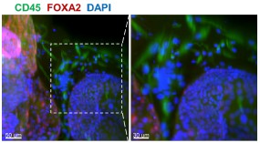
(1) Previous comments raised concerns about the feasibility of robustly passaging assembloid structures - comprising epithelial, stromal and immune cells - under epithelial growth conditions. The authors responded by stating that they optimized the expansion medium with a stromal cell-promoting factor. Additionally, rather than conducting scRNA-seq on both early and late passages (P6-P10) as suggested, they performed immunofluorescence staining, which confirmed the persistence of stromal cells at passage 6. However, the presence of immune cells was not addressed. Confirmation of their presence is essential for all further claims. Moreover, a more zoomed-out view of the immunostaining would help clarify the overall cellular composition across the entire well and facilitate comparison with corresponding brightfield images.
Whole-mount immunofluorescence of the 6th - generation assembloids revealed that CD45<sup>+</sup> immune cells surrounded FOXA2<sup>+</sup> glands, with a more zoomed-out view provided.
Author response image 1.
Whole-mount immunofluorescence showed that CD45<sup>+</sup> cells (immune cells) were arranged around the glandular spheres that were FOXA2<sup>+</sup>. Scale bar =50 μm (left) and 30 μm (right).
In their response, the authors mention using the first three passages to ensure optimal cell diversity and viability. However, the manuscript states that 'assembloids derived from the first generation are used for experiments' (line 106). This discrepancy must be clarified.
Thank you for your suggestion. We have revised the relevant content to “The assembloids derived from the first three generation are used for experiments” (Line 90-91).
(2) The authors have made a commendable effort to bring more focus to the manuscript, which has improved readability.
We thank you for your insightful suggestions, which have greatly improved the quality of our manuscript.
(3) The "embryo implantation" part remains very unconvincing. How did authors define "the blastoids could grow within the endometrial assembloids and interact with them"? What did they mean with "grow"? Did blastoids further differentiate? Normally, blastoids cannot further "grow". "Survival rates of blastoids" is not equal to "growth". It is not clear how the survival rate was quantified. Besides, regarding the "interaction rates", how did authors define and quantify it? Actually, blastoids are able to attach to Matrigel efficiently (even without any endometrial cells), so authors cannot simply define the "interaction" as the co-localization of blastoids and assembloids via brightfield images. In addition, for the assembloids as the 3D structures grow in the Matrigel, the epithelial parts are normally apical-in, while the blastoids attach to the apical (lumen) side of the epithelial cells, so physiologically, blastoids should interact with the apical part of the epithelial cells instead of the outside of the assembloids.
(1) What did they mean with "grow"? Did blastoids further differentiate?
On the one hand, volume and morphology undergo continuous dynamic changes; on the other hand, only the inner cell mass and trophectoderm exist at the blastocyst stage, with the ICM further differentiating into OCT4<sup>+</sup> epiblast and GATA6<sup>+</sup> hypoblast.
(2) Survival rates of blastoids" is not equal to "growth". It is not clear how the survival rate was quantified.
The definition of "survival rate" is as follows: morphologically, the blastocoel remains noncollapsed and the cell boundaries are distinct (with no obvious cell detachment); molecularly, the markers of epiblast, hypoblast and trophectoderm are expressed. The survival rate is calculated as the ratio of viable embryoids to the total number of embryoids.
(3) Besides, regarding the "interaction rates", how did authors define and quantify it? Actually, blastoids are able to attach to Matrigel efficiently (even without any endometrial cells), so authors cannot simply define the "interaction" as the co-localization of blastoids and assembloids via brightfield images.
The criteria for determining interaction include not only attachment between the blastoids and assembloids observed via brightfield images, but also their sustained tight adhesion against external mechanical perturbations (e.g., medium replacement, immunostaining procedures).
(4) In addition, for the assembloids as the 3D structures grow in the Matrigel, the epithelial parts are normally apical-in, while the blastoids attach to the apical (lumen) side of the epithelial cells, so physiologically, blastoids should interact with the apical part of the epithelial cells instead of the outside of the assembloids.
You are absolutely correct. In vivo, the embryo indeed makes initial contact with the apical side of the epithelial cells. The introduction of the blastoid co-culture model herein is intended to demonstrate that this receptive endometrial assembloids can better support blastoid growth and development.
(4) Previous comments highlighted the absence of distinct shifts in gene expression profiles between SEC assembloids and WOI assembloids, which contrasts with findings from primary endometrial tissue reported by Wang et al. (2020). While the authors have expanded their analysis using the Mfuzz algorithm and identified changes in mitochondria- and cilia-associated genes, the manuscript still lacks evidence of significant transcriptional changes in key WOI marker genes, as described in Wang et al. This discrepancy must be addressed and discussed in greater depth to clarify the biological relevance of their model.
The endometrium in vivo involves complex crosstalk among multiple cell types and is tightly regulated by the hypothalamic-pituitary-ovarian (HPO) axis, thus exhibiting distinct shifts in gene expression during the peri-implantation period.
In our in vitro model, alterations in mitochondria- and cilia-related genes were observed, which to a certain extent demonstrates that these window of implantation (WOI) assembloids possess receptive-phase characteristics and can be employed to investigate WOI-associated scientific questions or conduct in vitro drug screening.
However, substantial efforts are still required to optimize the current model for fully recapitulating the dynamic changes in endometrial gene expression across different phases in vivo, and this aspect is further addressed in the Limitations section of our discussion (Line 342-353).
“However, our WOI endometrial assembloids also exhibit some limitations. It is undeniable that the assembloids cannot perfectly replicate the in vivo endometrium, which comprises functional and basal layers with a greater abundance of cell subtypes, under superior regulation by hypothalamic-pituitary-ovarian (HPO) axis. Specifically, stromal and immune cells are challenging to stably passage, and their proportion is lower than in the in vivo endometrium. While the in vivo peri-implantation period exhibits intricate gene expression dynamics driven by systemic regulation, our models only partially recapitulate these changes, primarily in mitochondria- and cilia-associated genes. Nevertheless, to some extent, these WOI assembloids possess receptivity characteristics and can be utilized for investigating receptivity-related scientific questions or conducting in vitro drug screening. Further refinements are required to fully simulate the dynamic endometrial gene expression patterns across all menstrual cycle stages. We are looking forward to integrating stem cell induction, 3D printing, and microfluidic systems to modify the culture environment.”
(5) In the authors' response document, they present data integrating their results with those of Garcia Alonso et al. (2021). However, these integrated analyses are not included in the revised manuscript (which should be, if answering a major concern).
Thanks for your valuable suggestions. We have now integrated the findings of Garcia Alonso et al. (2021) into the revised manuscript (Line 132) and Figure S2E–F.
(8) Fig 2D: The authors have clarified that CD45+ staining is used. However, they have not yet adapted the typo in the figure legend of the right picture.
Thanks for your thorough review. The left panel of Figure 2D is stained with CD45 to label immune cells, while the right panel is stained with CD44. These details have been clearly indicated in both the manuscript and the figure legend.
(9) All quantification analyses (as described in the authors' response document) should be clearly described in the Materials & Methods section.
Thanks for your valuable suggestions. All quantification analyses have now been added to the Supporting Materials and Methods section (Line 94-104, Line 110-111, Line 241244).
(10) The authors have provided clarification regarding their method for quantifying immunofluorescence staining (e.g., OLFM4 expression in Fig. 3C) in their response document. However, these methodological details are not included in the revised manuscript. It is important that such information is incorporated into the manuscript itself to ensure transparency and reproducibility for others.
Thanks for your valuable suggestions. All quantification analyses have now been added to the Supporting Materials and Methods section (Line 94-104).
(13) It is needed to include the author's response to the comment about literature showing the opposite of increased number of cilia during the WOI into the discussion part of the paper.
We appreciate your suggestions. The relevant content has now been added to the Discussion section (Lines 319–323).
(14) In the authors' response, they explain the difference between pinopodes and microvilli. They should include this explanation briefly in the manuscript. Moreover, Fig. 3F lacks a picture of cilia structure in CTRL condition. In addition, the structures that are indicated as cilia with an orange arrow seem to not be attached to the endometrial cells (anymore). It would be useful to show another more representative picture for the cilia.
(1) Thank you for your valuable suggestions. The distinction between pinopodes and microvilli has now been added to the Supporting Materials and Methods section (Line 230-236).
(2) You are probably referring to Figure 2F—we did not observe ciliary structures in the CTRL group.
(3) The cilia structure was visualized via transmission electron microscopy (TEM), which requires ultrathin sectioning. Thus, the cilia shown in the image correspond to a single cross-section of the captured assembloids. Owing to technical limitations, three-dimensional visualization of cilia on the cells cannot be achieved.
(17) The results on co-culturing blastoids with the WOI assembloids is not convincing. The blastoids are exposed to the basolateral side of the endometrial epithelial cells, while in vivo, blastocysts interact with the apical side of the endometrial epithelial cells first (apposition and attachment), followed by invasion into the endometrium. This means that the interaction shown here is not physiological. Therefore, it is not justified to say that this platform holds promise to investigate maternal-fetal interactions.
We agree with your perspective that discrepancies exist between this model and the physiological processes in vivo. However, such differences do not negate the scientific value of the model.
The core merit of this study lies in the successful establishment of co-culture systems for blastoids and WOI assembloids. Notably, genuine cross-talk occurs between the two components, thereby providing a practical and operational tool for subsequent research.
Although the current contact orientation differs from that observed in vivo, future optimization of the cell culture protocol (via modulation of cell polarity) will enable the model to better recapitulate physiological conditions. Therefore, the innovation and operability of this model within specific research contexts still render it a robust platform for investigating maternal-fetal interactions.
Overall, it is highly recommended that the authors carefully review the manuscript for grammatical errors, inconsistencies and issues with scientific phrasing. The language throughout the text requires substantial editing to improve clarity, readability and precision.
We appreciate your suggestions. A full manuscript check was performed to rectify grammatical errors, inconsistencies, and inappropriate scientific phrasing, with further language refinement by a native English-speaking specialist.
Fig 1A: This overview is unclear. How many days do the assembloids grow before being stimulated with hormones? Are CTRL assembloids only kept in culture until day 2 and SEC and WOI assembloids until day 8? This is also not clear form the Materials and Methods section. Should be clarified.
Thanks for your valuable suggestions. We have now updated the overview (Figure 1A) and Materials and Methods section (Line 370-371, Line 379-381).
“Hormonal treatment was initiated following the assembly of the endometrial assembloids (about 7-day growth period).”
“The CTRL group was cultured in ExM without hormone supplementation and subjected to parallel culture for 8 days along with the two aforementioned groups.”
Fig 1B: From these brightfield images, it appears that the size of the assembloids remains relatively consistent from Day 0 to Day 3 and up to Day 11 (especially in CTRL). However, in Fig S1A, the assembloids on Day 11 appear significantly larger compared to those on Day 2 (or Day 4). Authors should clarify this discrepancy (since both of the figures are shown as "brightfield of endometrial assembloids").
You are probably referring to the observation that the assembloids at Day 11 in Fig. S1A are smaller in size than those at Day 2 (or Day 4) in Fig. 1B. This discrepancy arises because the time points in Fig. 1B are calculated starting from the initiation of hormone treatment for the SEC and WOI groups, rather than from the beginning of the overall culture as in Fig. S1A. In addition, assembloids exhibit size variability during the same culture period due to individual heterogeneity.
To eliminate ambiguity, we have now labeled “Hormone Day 0, Day 2, Day 8” in Fig. 1B and revised the corresponding figure legend to read: “Endometrial assembloids from the CTRL, SEC, and WOI groups, which were subjected to hormone treatment on Days 0, 2, and 8, exhibited comparable growth patterns throughout the culture period.”
Fig 2G: authors still used the description "organoids" here instead of "assembloids".
We appreciate your careful review. Corrections have been made accordingly.
Fig. 3C: For the OLFM4 staining quantification, in the Y-axis authors wrote "proportion of OLFM4 (+) cells (OLFM4 (+)/total", but in the rebuttal letter they mention "its fluorescence intensity (quantified as mean grey value) was significantly stronger in both the SEC and WOI groups compared to the CTRL group". This is confounding and should be clarified.
We apologize for incorrectly writing "fluorescence intensity" in the rebuttal letter; the correct term should be the "proportion of OLFM4 (+) cells (OLFM4 (+)/total)" as shown in Fig. 3C.
Fig 5D: Acetyl-α-tubulin is the marker of ciliated cells and should be expressed in the cilia instead of the whole cells. It is very strange to quantify as "mean fluorescence intensity (acetyl-αtubulin/DAPI)" to assess the cilia. Please clarify.
Thank you for your insightful comment. To clarify, the ratio "mean fluorescence intensity (acetyl-α-tubulin/DAPI)" was calculated within individual acetyl-α-tubulin<sup>+</sup> ciliated cells. Acetyl-αtubulin fluorescence was normalized to the DAPI signal of the same cell nucleus, not the wholecell population. This corrected for variations in cell number and staining efficiency to ensure data accuracy.
Fig 5F: it is very bizarre that unciliated epithelium was transformed from ciliated epithelium, and CTRL was transformed from SEC and WOI. Should be clarified and discussed.
Pseudotime analysis sorts discrete cells along a "pseudotime axis" based on similarities and differences in cellular gene expression, thereby simulating cell state transitions.
Ciliated epithelium → unciliated epithelium: During the menstrual cycle, ciliated and unciliated epithelia undergo mutual transformation from the secretory phase (or mid-secretory phase) to the menstrual phase, and then to the proliferative phase. Here, we demonstrate the transition of ciliated cells to unciliated cells from the SEC and WOI stages to the CTRL stage.
Notably, the two cell types coexist, and what is presented here merely reflects a transformation trend. Relative content has been incorporated into the Discussion section (Line 319-321).
“Throughout the menstrual cycle, ciliated and unciliated epithelia undergo mutual transformation from the secretory phase (or mid-secretory phase) to the menstrual phase, and then to the proliferative phase.”
Fig 5H: To show "enhanced invasion ability", authors must provide some quantification and statistic analysis. It is very hard to see the difference between the CTRL and SEC regarding ROR2Wnt5A.
We appreciate your suggestion. Quantification and statistic analysis have been added to Figure 5H.
Fig 6A: please elaborate the "mIVC1" and "mIVC2" in the figure legends.
Additions have been made to the figure legends accordingly, as follows: "mIVC1: modified In Vitro Culture Medium 1; mIVC2: modified In Vitro Culture Medium 2."
Fig S1D: Is the PAS staining also done in CTRL assembloids? In addition, it is stated that the assembloids secrete glycogen because of a positive PAS staining, while it could also be neutral mucins, glycoproteins, etc, which are all detected by PAS staining. So, the authors should be more careful in stating that it is glycogen, or a PAS staining with diastase digestion should be done.
The PAS staining results for the CTRL group are presented in Fig. S1I. In addition, results of PAS staining with diastase digestion are included in Figure S1.
Line 120: references?
The reference has been added accordingly.
Line 178: The term 'Endometrial Receptivity Test (ERT)' is used. Do the authors mean Endometrial Receptivity Analysis (ERA) test? ERA is the commonly used abbreviation for this test. Moreover, the authors describe ERA as 'a kind of gene analysis-based test.' This should be rephrased more scientifically correct.
Thank you for your valuable suggestion. We have revised the term to ERA, and modified the phrase "a kind of gene analysis-based test" to "gene expression profiling-based diagnostic assay" (Lines 160–163).
“We performed Endometrial Receptivity Analysis (ERA), a gene expression profiling-based diagnostic assay that integrates high-throughput sequencing and machine learning to quantify the expression of endometrial receptivity-associated genes.”
Line 83: assemblies à assembloids
We appreciate your suggestion. The text has been updated to “the endometrial assembloids progressed from epithelial organoids, to assemblies of epithelial and stromal cells and then to stem cell-laden 3D artificial endometrium”.
The Materials and Methods section currently lacks the needed details. Authors should substantially expand this section to clearly describe all experimental and analytical procedures, including, aùmong others, immunofluorescence staining, quantification methods, bioinformatics analyses and statistical approaches. Providing comprehensive methodological information is essential.
A detailed description of these methods is provided in the Supporting Materials and Methods section.
Reviewer #2 (Recommendations for the authors):
The revised manuscript is much improved in clarity, focus, and experimental support. The authors have thoughtfully addressed the major concerns from the previous review. In particular, the logic and flow of the paper are clearer, it now guides the reader through the rationale (constructing a WOI model), the comparative analysis against in vivo tissue and simpler organoids, and the key features that distinguish the WOI assembloid. The added functional validation (especially the blastoid co-culture experiment) significantly strengthens the work by showing a tangible outcome of "receptivity" beyond molecular profiling. The distinction between the standard secretory-phase organoid and the WOI assembloid is now more convincing, as the authors highlight several specific differences in morphology (more cilia, pinopodes), metabolism, and implantation success that favor the WOI model. The manuscript also reads cleaner with the bioinformatic sections condensed to the most important findings (excess detail was trimmed or moved to supplements) and the rationale for gene/pathway selection explicitly stated.
The manuscript has been significantly strengthened through the addition of functional assays (like the blastoid co-culture), clearer transcriptomic and proteomic data, and detailed analyses of hormone treatments, cilia biology, and stromal and immune cell behavior in early passages. These updates confirm that the WOI assembloid supports embryo attachment and outperforms standard secretory organoids, while integrating external references and clarifications on terminology. Minor suggestions remain, such as clarifying statistical significance and adding functional interpretations for certain observations, but overall, the manuscript is now more robust and biologically convincing.
Remaining points for clarification: There are a few minor points that still merit attention:
- Use of the Endometrial Receptivity Test (ERT): As previously mentioned, if the authors have ERT data for the SEC organoid group, including that information would further support the claim that the WOI assembloid is uniquely receptive. If not, it would be helpful to add a statement clarifying that the ERT was employed specifically as a confirmatory test for the WOI assembloids, rather than as a comparative measure across all groups.
Thank you for your valuable suggestion. We have now supplemented the description in the Supporting Materials and Methods section (Lines 160–162) as follows: “ERA was employed specifically as a confirmatory test for the WOI assembloids, rather than as a comparative measure across all groups.”
- Because the assembloids are created from primary tissue samples, it would be helpful to briefly comment on how consistent the findings were across different patient-derived samples. For example, did all biological replicates show similar expression of receptivity markers and comparable capacity to support blastoid attachment? Although this seems implied, including a sentence in the Methods or Results sections that specifies the number of donor lines tested would help readers assess the model's variability and reproducibility.
We appreciated your advice. The relevant statement has been added to the Supporting Materials and Methods section. (Line 312-313).
“All biological replicates (fourteen individuals) of endometrial assembloids show similar expression of receptivity markers and comparable capacity to support blastoid attachment.”
- The authors mention promising future directions, such as integrating 3D printing and microfluidics to further enhance the model, which is an excellent forward-looking statement. It would also be valuable to suggest the inclusion of additional cell types, like more robust immune cell populations or endothelial components, as future improvements to create an even more comprehensive model of the endometrial lining.
Thank you for your valuable suggestion. 3D printing and microfluidics serve as approaches for introducing multiple cell types. We have supplemented the following statement in the manuscript: “We are looking forward to integrating stem cell induction, 3D printing, and microfluidic systems to modify the culture environment.” (Line 352-353).
We are grateful for your valuable feedback and constructive criticism, which have helped us improve the quality of our work in terms of content and presentation. We have diligently revised the manuscript and made necessary changes. Here, we have attached the revised manuscript, figures, and all supplementary materials for your re-evaluation. Thank you again for your continued support and look forward to your favorable decision.
État des Lieux Scientifique des Thérapies Manuelles : Entre Mythes et Réalités
Ce document de synthèse analyse l'état actuel des connaissances scientifiques concernant les thérapies manuelles (kinésithérapie, ostéopathie, chiropraxie, étiopathie), avec un accent particulier sur le mal de dos, principal motif de consultation.
Les points saillants sont les suivants :
• Le primat du mouvement : La science moderne démontre que le traitement le plus efficace contre la lombalgie est le mouvement actif.
Les thérapies passives ne doivent pas être utilisées de manière isolée.
• Obligations légales et déontologiques : Contrairement aux pseudomédecines, la kinésithérapie est encadrée par l'obligation d'utiliser des moyens conformes aux « données acquises de la science », un principe juridique ancré depuis l'arrêt Mercier de 1936.
• Déconstruction des mythes : Les concepts de « vertèbre déplacée » ou de « bassin décalé » sont des vues de l'esprit sans réalité anatomique.
La palpation manuelle, bien que rassurante, manque de fiabilité scientifique pour établir un diagnostic de texture ou de blocage.
• Risques et conséquences sociales : Au-delà de l'effet placebo ou contextuel, certaines manipulations (notamment cervicales) présentent des risques graves comme l'accident vasculaire cérébral (AVC).
De plus, ces pratiques peuvent parasiter les messages de santé publique et altérer la littératie en santé des patients.
--------------------------------------------------------------------------------
L'approche médicale de la lombalgie a radicalement changé au cours des trente dernières années, passant d'une logique de repos à une logique d'action.
• 1986 : Une étude du New England Journal of Medicine suggère que deux jours de repos au lit sont plus bénéfiques que sept jours.
• 1995 : Une étude pivot démontre que le groupe "témoin" (continuant à vivre normalement) récupère mieux que les groupes soumis à un repos strict ou à des exercices trop prudents.
• 2019 : La Haute Autorité de Santé (HAS) et l'Assurance Maladie lancent des recommandations officielles : « Le bon traitement, c'est le mouvement ».
Les thérapies passives isolées sont déclarées inefficaces sur l'évolution de la lombalgie.
Contrairement aux idées reçues, des activités comme la course à pied améliorent la physiologie discale.
L'alternance de pressions et dépressions (environ 1 Hz) lors de la course permet d'hydrater les disques intervertébraux. Statistiquement, les coureurs de fond souffrent moins du dos que les autres sportifs.
--------------------------------------------------------------------------------
La distinction entre kinésithérapie et thérapies alternatives repose sur un fondement juridique historique.
Ce tournant de la Cour de cassation a établi trois principes majeurs :
1. Le contrat de soins : Il existe un lien contractuel entre le soignant et le patient.
2. L'obligation de moyens : Le soignant n'a pas d'obligation de résultat (guérison), mais doit mettre en œuvre tous les moyens nécessaires.
3. Les données acquises de la science : Les moyens choisis doivent être conformes aux connaissances scientifiques actuelles.
Le code de déontologie impose aux kinésithérapeutes d'abandonner les pratiques invalidées. Par exemple :
• Bronchiolite : La kinésithérapie respiratoire pédiatrique n'est plus recommandée depuis 2019 pour les nourrissons sains, car le bénéfice est jugé insuffisant par rapport au caractère traumatisant du soin.
• Massage : Son usage est désormais limité (cicatrices, œdèmes) et n'est plus recommandé comme traitement de première intention pour le mal de dos.
--------------------------------------------------------------------------------
La science démontre que le sens tactile des praticiens est sujet à l'illusion.
• Manque de fiabilité : Deux évaluateurs sont rarement d'accord sur la texture (dur/mou) ou le caractère « bloqué » d'un tissu.
• Précision anatomique : En palpant une structure évidente sous la peau, l'erreur moyenne est de 5 cm.
• Impossibilité mécanique : Il est impossible de mobiliser une seule vertèbre de façon isolée ; une manipulation en impacte au minimum trois.
Les thérapies manuelles produisent un effet antalgique réel mais transitoire :
• Distraction sensorielle : Le système nerveux privilégie les sensations tactiles, de chaud ou de froid sur la douleur. C'est un effet à court terme (quelques minutes à quelques heures).
• Effet contextuel : Le rituel de la consultation, l'attention portée par le praticien et la régression naturelle vers la moyenne (la douleur diminue souvent d'elle-même au moment où l'on consulte) renforcent l'illusion d'efficacité.
--------------------------------------------------------------------------------
Les thérapies comme l'ostéopathie ou la chiropraxie reposent sur le vitalisme, une philosophie du XIXe siècle postulant l'existence d'une « force vitale » non physique.
| Discipline | Origine | Fondements Idéologiques | État actuel en Europe | | --- | --- | --- | --- | | Ostéopathie | A.T. Still (1874) | "Le corps est la pharmacie de Dieu". Flux sanguin synonyme de santé. | Branche "puriste" (Littlejohn) très présente, axée sur le crânio-sacré et le fluidique. | | Chiropraxie | D.D. Palmer (1895) | Système nerveux central comme maître du corps. Recours aux manipulations à haute vélocité (faire craquer). | Pratique restée proche des concepts originels, avec une forte présence sur les réseaux sociaux. | | Étiopathie | C. Trédaniel (Fr) | Recherche de l'origine de la pathologie dans l'ajustement articulaire. | Très similaire à l'ostéopathie, sans distinction scientifique réelle. |
Note sur l'exception américaine : Aux États-Unis, l'ostéopathie s'est médicalisée suite au rapport Flexner (1910). Les "DO" y sont des médecins généralistes qui ne pratiquent quasiment plus de thérapie manuelle, contrairement à la branche européenne restée mystique.
--------------------------------------------------------------------------------
• Risques graves : Les manipulations cervicales peuvent provoquer des dissections de l'artère vertébrale, entraînant des AVC ou le syndrome de "Locked-in" (paralysie totale avec conscience préservée).
• Erreurs de diagnostic : Le recours direct à ces thérapies sans avis médical peut retarder la prise en charge de pathologies graves (ex: fractures non détectées).
Le "vernis médical" utilisé par ces disciplines (mots tels que « diagnostic », « anamnèse », « consultation ») crée une confusion chez les patients :
• Atteinte à la littératie en santé : En ancrant des concepts erronés (vertèbre déplacée, jambe plus courte), les praticiens créent une dépendance et une peur de bouger (kinésiophobie).
• Facteurs sociaux : Le principal facteur de persistance d'une lombalgie n'est pas mécanique, mais lié à l'insatisfaction au travail ou à des problèmes sociétaux. Les thérapies manuelles, en se focalisant sur le "crack and go", ignorent cette complexité.
Si les thérapies manuelles offrent un soulagement temporaire et un confort relationnel, elles ne constituent pas une solution de fond au mal de dos.
La science préconise une approche centrée sur l'éducation thérapeutique, la gestion de la motivation et, impérativement, le mouvement actif du patient.
Analyse de la Rhétorique Complotiste : Mécanismes, Discours et l'Allégorie du « Mouton »
Ce document de synthèse analyse les recherches et les réflexions de Loïc Massaia, vulgarisateur pour le projet Utopia, concernant la rhétorique employée dans les milieux complotistes.
Il détaille les structures argumentatives, les fonctions psychologiques du discours et l'usage spécifique de l'insulte « mouton » comme outil de distinction sociale et de clôture du débat.
L'analyse de la rhétorique complotiste révèle un système de communication visant moins à établir une vérité qu'à asseoir un ascendant sur l'auditoire.
Cette rhétorique se caractérise par une structure circulaire (tautologique) et un recours systématique à l'essentialisme.
L'usage de termes comme « mouton » remplit une triple fonction : une attaque ad personam pour éviter le débat de fond, une accusation de complicité passive, et un mécanisme de distinction permettant de renforcer l'estime de soi du locuteur.
En s'affranchissant des règles du « débat sain », le discours complotiste s'établit comme un système fermé où la conclusion (l'existence d'un complot) est déjà contenue dans les prémisses.
-------------------------------------------------------------------------------
Le document propose de définir la rhétorique comme l'ensemble des moyens mis en œuvre dans un discours pour convaincre, briller, manipuler ou obtenir un ascendant sur autrui.
Une définition complémentaire la décrit comme la « négociation de la différence entre les individus sur une question donnée ».
Dans le cadre du complotisme, les expressions récurrentes peuvent être classées selon quatre dimensions principales :
| Dimension | Exemples de phrases types | Objectif recherché | | --- | --- | --- | | Accusatoire | « Journalopes », « Merdias », « On ne vous dit pas tout » | Discréditer les sources d'information officielles. | | Incitatoire | « Faites vos propres recherches », « Réveillez-vous » | Pousser l'interlocuteur à adopter la même conclusion par une illusion d'autonomie. | | Négation du hasard | « Coïncidence ? Je ne crois pas », « Tout est lié » | Refuser la contingence au profit d'un dessein caché. | | Surconfiance et Distinction | « Tous des moutons », « On avait raison » | Se placer au-dessus de la « masse » ignorante. |
--------------------------------------------------------------------------------
Pour évaluer la solidité d'un argument, le document mobilise le modèle de Toulmin, qui identifie les composants d'une argumentation optimale :
1. Données : Les informations de base.
2. Conclusion : Ce que l'on veut démontrer.
3. Justifications : Le lien logique entre données et conclusion.
4. Fondement : Ce qui rend la justification solide et acceptée.
5. Réfutation : L'intégration des limites et des conditions qui pourraient contredire l'argument.
L'analyse montre que le discours complotiste omet généralement la réfutation.
Par exemple, l'argument consistant à dire que le gouvernement est une secte parce qu'il lutte contre les dérives sectaires (pour étouffer la dissidence) s'effondre si l'on introduit d'autres facteurs de distinction entre État et secte.
Le discours complotiste est décrit comme un système fermé ou une tautologie.
Il repose sur l'essentialisation : on décrète que la « nature » profonde d'une entité (le gouvernement, les élites) est malveillante.
Dès lors, toute action de cette entité, même positive en apparence, est interprétée comme une preuve supplémentaire de sa malveillance.
Le complot existe nécessairement au départ pour expliquer les faits qui servent ensuite à prouver l'existence du complot.
--------------------------------------------------------------------------------
L'expression « tous des moutons » est un idiotisme animalier présent dans plusieurs langues (français, italien, anglais, polonais).
L'image du mouton qui suit aveuglément remonte notamment à Rabelais (l'épisode des moutons de Panurge), où les animaux sautent à l'eau et meurent simplement parce que le premier a sauté.
Cela souligne une dimension « naturelle » ou essentialiste de l'animal : le besoin de suivre.
1. L'identification du comploteur : S'il y a des moutons, il y a nécessairement un « berger » ou un « maître » (le comploteur).
2. L'accusation de complicité : Les non-complotistes sont jugés idiots, mais aussi complices par leur passivité.
3. Le besoin de distinction : Se déclarer « non-mouton » permet de s'extraire de la masse. Selon les travaux d'Anthony Lantian (2015), l'adhésion aux théories du complot serait un moyen de rehausser une estime de soi initialement basse en se sentant détenteur d'un savoir supérieur.
--------------------------------------------------------------------------------
L'usage de l'insulte « mouton » est qualifié d'argument ad personam.
Théorisée par Schopenhauer, cette tactique consiste à attaquer l'individu plutôt que ses arguments pour mettre fin à une discussion que l'on ne peut pas gagner sur le fond.
En s'appuyant sur les travaux de Levi Hedge (XIXe siècle), le document identifie trois règles fondamentales d'un débat sain systématiquement violées par la rhétorique complotiste :
• Règle n°4 : Interdiction des attaques personnelles.
• Règle n°5 : Interdiction d'accuser l'adversaire de mobiles cachés.
• Règle n°7 : La vérité doit être le but, non la victoire. L'usage du ridicule ou de la raillerie (traiter l'autre de mouton) est une violation de cette règle.
Toutefois, le document souligne que ces dérives ne sont pas l'apanage des complotistes ; elles se retrouvent fréquemment dans tout débat public où l'objectif des participants est de « gagner » plutôt que de chercher la vérité.
--------------------------------------------------------------------------------
En conclusion, le document invite à une réflexion sur la nature même de la critique du complotisme.
Si l'on définit la rhétorique complotiste comme étant « par nature » une tautologie basée sur un essentialisme, on court le risque de produire soi-même un discours fermé et essentialiste.
Cette mise en abyme suggère que l'analyse du complotisme doit elle-même rester vigilante quant à ses propres structures argumentatives pour ne pas tomber dans les travers qu'elle dénonce.
Synthèse Clinique : Comprendre et Accompagner la Cooccurrence TSA-TDAH (ODHD)
Ce document propose une analyse approfondie de la cooccurrence entre le Trouble du Spectre de l'Autisme (TSA) et le Trouble du Déficit de l'Attention avec ou sans Hyperactivité (TDAH), un profil souvent désigné sous l'acronyme anglo-saxon « ODHD ».
Longtemps ignorée par les classifications officielles (notamment avant le DSM-5 en 2013), cette double problématique est aujourd'hui reconnue comme une entité clinique à part entière, et non une simple addition de symptômes.
Les points clés de cette analyse incluent :
• Prévalence élevée : Plus de 40 % des individus avec un TSA présentent un TDAH associé.
• Complexité clinique : La combinaison des deux troubles entraîne une sévérité accrue des symptômes, une fatigue majeure (burnout autistique) et des profils sensoriels complexes.
• Prise en charge spécifique : L'approche doit être multidisciplinaire, privilégiant la psychoéducation et une pharmacologie prudente, tout en évitant le recours systématique aux antipsychotiques.
• Changement de paradigme : Il est crucial de passer d'une vision centrée sur le symptôme à une vision axée sur le fonctionnement global et la qualité de l'environnement.
--------------------------------------------------------------------------------
Avant 2013, le DSM-5 interdisait formellement le double diagnostic TSA et TDAH. Pourtant, la pratique clinique révélait déjà des patients présentant des caractéristiques marquées des deux troubles. Depuis la levée de cette interdiction, la littérature scientifique et l'expérience de terrain confirment une imbrication fréquente.
Les données actuelles mettent en évidence une asymétrie dans la comorbidité :
• TSA avec TDAH : Plus de 40 % des personnes autistes répondent également aux critères du TDAH.
• TDAH avec TSA : Environ 13 % à 20 % des personnes TDAH présentent des traits autistiques associés.
Il est impératif de distinguer l'origine des symptômes pour éviter un empilement erroné de diagnostics. Par exemple :
• Les difficultés sociales du TDAH sont souvent liées à l'impulsivité ou l'inattention, tandis que dans le TSA, elles relèvent de la cognition sociale.
• Les troubles attentionnels du TSA sont souvent la conséquence d'une hyper-sensorialité ou d'intérêts restreints plutôt que d'un mécanisme TDAH intrinsèque.
--------------------------------------------------------------------------------
L'association des deux troubles (ODHD) crée un tableau singulier où les symptômes s'influencent mutuellement, augmentant la sévérité globale.
| Domaine de fonctionnement | Impact de la cooccurrence TSA + TDAH | | --- | --- | | Fonctions Exécutives | Difficultés plus marquées (inhibition, flexibilité, attention) ; profil proche du TDAH isolé mais plus sévère. | | Cognition Sociale | Difficultés sociales accrues, contact visuel moindre et peu d'amélioration spontanée avec le temps. | | Sensorialité | Cumul des hypersensibilités ; profil sensoriel complexe et particulièrement intense. | | Santé Mentale | Risque accru de troubles dépressifs, troubles du sommeil, épuisement majeur et burnout autistique. | | Adaptation | Précarité économique plus importante et difficultés psychosociales majeures. |
Un point crucial de l'analyse est la distinction entre avoir un fonctionnement neurodivergent et présenter un trouble. Le trouble n'apparaît que lorsqu'il y a une répercussion fonctionnelle négative. Cette répercussion est étroitement liée à la qualité environnementale (par exemple, la personnalité d'un enseignant ou l'adaptation d'un poste de travail).
--------------------------------------------------------------------------------
La psychoéducation doit être « sextuple » (incluant l'enfant, les parents et la fratrie). Ses objectifs sont de :
• Donner du sens aux symptômes.
• Mettre fin aux idées reçues et aux préjugés (notamment ceux des soignants).
• Réduire l'auto-stigmatisation et la culpabilité.
• Limiter le "masking" (suradaptation permanente), qui est une cause majeure d'épuisement et de burnout.
Le recours au méthylphénidate est possible mais nécessite une expertise clinique fine :
• Sensibilité accrue : Les patients TSA sont souvent hyper-sensibles aux substances (perception fine des changements corporels).
• Posologie : Il est recommandé de commencer par des doses très faibles (ex: 5 mg) et d'augmenter de manière très progressive.
• Vigilance : Surveiller l'augmentation potentielle des stéréotypies ou de l'irritabilité.
• Critique des pratiques : Le document dénonce comme une « hérésie » l'usage de première intention des antipsychotiques (type Haldol ou Risperdal) en France, au détriment du méthylphénidate.
L'hygiène de vie et le corps sont des leviers fondamentaux :
• Hygiène de vie : Régime méditerranéen, sommeil de qualité et régulation de l'exposition aux écrans.
• Activité physique : Présente une efficacité majeure prouvée par la littérature pour la régulation du TDAH.
• Régulation émotionnelle : Utilisation d'outils de cohérence cardiaque (ex: RespiRelax) pour agir sur le système nerveux autonome.
• Médiations alternatives : La musicothérapie et la danse-thérapie sont particulièrement efficaces car elles passent par les fréquences et le corps plutôt que par le langage verbal.
--------------------------------------------------------------------------------
Il est essentiel de ne pas réduire l'individu à ses symptômes mais de reconnaître les forces inhérentes à ces profils.
• Forces du TDAH : Empathie, créativité (issue des stratégies d'adaptation développées), curiosité, enthousiasme, intuition et rapidité.
• Forces du TSA : Précision, sérieux, honnêteté, respect des horaires et sens du détail.
• Lecture évolutionniste : La persistance des troubles du neurodéveloppement (TND) dans l'évolution humaine suggère leur utilité sociale. Par exemple, le TDAH pour l'exploration et la résolution de problèmes rapides, et le TSA pour la vigilance et l'expertise technique au sein d'un groupe.
Le projet « Atipy Friendly » illustre la transition nécessaire vers une société (notamment l'université) capable de s'adapter à la singularité de ces fonctionnements, plutôt que d'exiger une suradaptation systématique des personnes concernées.
--------------------------------------------------------------------------------
Le profil TSA-TDAH (ODHD) nécessite une attention particulière et une coordination accrue entre les professionnels (psychomotriciens, pédopsychiatres, éducateurs).
L'enjeu n'est pas seulement de traiter des symptômes, mais de répondre aux besoins spécifiques de la personne pour favoriser son autonomie et sa qualité de vie, tout en valorisant les forces liées à sa neurodivergence.
THE AMERICAN YAWP Menu Skip to content HomeAbout Barbara Jordan – On the Impeachment of Richard Nixon (1974) Brookes print Casta painting Contributors How the Other Half Lived: Photographs of Jacob Riis Introduction Note on Recommended Readings Press Sample Feedback (@AmericanYawp) Teaching Materials TEST: 11/18/2025 Updates Who Pays for This? 6. A New Nation “The Federal Pillars,” from The Massachusetts Centinel, August 2, 1789. Library of Congress. *The American Yawp is an evolving, collaborative text. Please click here to improve this chapter.* I. IntroductionII. Shays’s RebellionIII. The Constitutional ConventionIV. Ratifying the ConstitutionV. Rights and CompromisesVI. Hamilton’s Financial SystemVII. The Whiskey Rebellion and Jay’s TreatyVIII. The French Revolution and the Limits of LibertyIX. Religious FreedomX. The Election of 1800XI. ConclusionXII. Primary SourcesXIII. Reference Material I. Introduction On July 4, 1788, Philadelphians turned out for a “grand federal procession” in honor of the new national constitution. Workers in various trades and professions demonstrated. Blacksmiths carted around a working forge, on which they symbolically beat swords into farm tools. Potters proudly carried a sign paraphrasing from the Bible, “The potter hath power over his clay,” linking God’s power with an artisan’s work and a citizen’s control over the country. Christian clergymen meanwhile marched arm-in-arm with Jewish leaders. The grand procession represented what many Americans hoped the United States would become: a diverse but cohesive, prosperous nation.1 Over the next few years, Americans would celebrate more of these patriotic holidays. In April 1789, for example, thousands gathered in New York to see George Washington take the presidential oath of office. That November, Washington called his fellow citizens to celebrate with a day of thanksgiving, particularly for “the peaceable and rational manner” in which the government had been established.2 But the new nation was never as cohesive as its champions had hoped. Although the officials of the new federal government—and the people who supported it—placed great emphasis on unity and cooperation, the country was often anything but unified. The Constitution itself had been a controversial document adopted to strengthen the government so that it could withstand internal conflicts. Whatever the later celebrations, the new nation had looked to the future with uncertainty. Less than two years before the national celebrations of 1788 and 1789, the United States had faced the threat of collapse. II. Shays’s Rebellion Daniel Shays became a divisive figure, to some a violent rebel seeking to upend the new American government, to others an upholder of the true revolutionary virtues Shays and others fought for. This contemporary depiction of Shays and his accomplice Job Shattuck portrays them in the latter light as rising “illustrious from the Jail.” Unidentified artist, Daniel Shays and Job Shattuck, 1787. Wikimedia. In 1786 and 1787, a few years after the Revolution ended, thousands of farmers in western Massachusetts were struggling under a heavy burden of debt. Their problems were made worse by weak local and national economies. Many political leaders saw both the debt and the struggling economy as a consequence of the Articles of Confederation, which provided the federal government with no way to raise revenue and did little to create a cohesive nation out of the various states. The farmers wanted the Massachusetts government to protect them from their creditors, but the state supported the lenders instead. As creditors threatened to foreclose on their property, many of these farmers, including Revolutionary War veterans, took up arms. Led by a fellow veteran named Daniel Shays, these armed men, the “Shaysites,” resorted to tactics like the patriots had used before the Revolution, forming blockades around courthouses to keep judges from issuing foreclosure orders. These protesters saw their cause and their methods as an extension of the “Spirit of 1776”; they were protecting their rights and demanding redress for the people’s grievances. Governor James Bowdoin, however, saw the Shaysites as rebels who wanted to rule the government through mob violence. He called up thousands of militiamen to disperse them. A former Revolutionary general, Benjamin Lincoln, led the state force, insisting that Massachusetts must prevent “a state of anarchy, confusion and slavery.”3 In January 1787, Lincoln’s militia arrested more than one thousand Shaysites and reopened the courts. Daniel Shays and other leaders were indicted for treason, and several were sentenced to death, but eventually Shays and most of his followers received pardons. Their protest, which became known as Shays’s Rebellion, generated intense national debate. While some Americans, like Thomas Jefferson, thought “a little rebellion now and then” helped keep the country free, others feared the nation was sliding toward anarchy and complained that the states could not maintain control. For nationalists like James Madison of Virginia, Shays’s Rebellion was a prime example of why the country needed a strong central government. “Liberty,” Madison warned, “may be endangered by the abuses of liberty as well as the abuses of power.”4 III. The Constitutional Convention The uprising in Massachusetts convinced leaders around the country to act. After years of goading by James Madison and other nationalists, delegates from twelve of the thirteen states met at the Pennsylvania state house in Philadelphia in the summer of 1787. Only Rhode Island declined to send a representative. The delegates arrived at the convention with instructions to revise the Articles of Confederation. The biggest problem the convention needed to solve was the federal government’s inability to levy taxes. That weakness meant that the burden of paying back debt from the Revolutionary War fell on the states. The states, in turn, found themselves beholden to the lenders who had bought up their war bonds. That was part of why Massachusetts had chosen to side with its wealthy bondholders over poor western farmers.5 James Madison, however, had no intention of simply revising the Articles of Confederation. He intended to produce a completely new national constitution. In the preceding year, he had completed two extensive research projects—one on the history of government in the United States, the other on the history of republics around the world. He used this research as the basis for a proposal he brought with him to Philadelphia. It came to be called the Virginia Plan, named after Madison’s home state.6 James Madison was a central figure in the reconfiguration of the national government. Madison’s Virginia Plan was a guiding document in the formation of a new government under the Constitution. John Vanderlyn, Portrait of James Madison, 1816. Wikimedia. The Virginia Plan was daring. Classical learning said that a republican form of government required a small and homogenous state: the Roman republic, or a small country like Denmark, for example. Citizens who were too far apart or too different could not govern themselves successfully. Conventional wisdom said the United States needed to have a very weak central government, which should simply represent the states on certain matters they had in common. Otherwise, power should stay at the state or local level. But Madison’s research had led him in a different direction. He believed it was possible to create “an extended republic” encompassing a diversity of people, climates, and customs. The Virginia Plan, therefore, proposed that the United States should have a strong federal government. It was to have three branches—legislative, executive, and judicial—with power to act on any issues of national concern. The legislature, or Congress, would have two houses, in which every state would be represented according to its population size or tax base. The national legislature would have veto power over state laws.7 Other delegates to the convention generally agreed with Madison that the Articles of Confederation had failed. But they did not agree on what kind of government should replace them. In particular, they disagreed about the best method of representation in the new Congress. Representation was an important issue that influenced a host of other decisions, including deciding how the national executive branch should work, what specific powers the federal government should have, and even what to do about the divisive issue of slavery. For more than a decade, each state had enjoyed a single vote in the Continental Congress. William Patterson’s New Jersey Plan proposed to keep things that way. The Connecticut delegate Roger Sherman, furthermore, argued that members of Congress should be appointed by the state legislatures. Ordinary voters, Sherman said, lacked information, were “constantly liable to be misled” and “should have as little to do as may be” about most national decisions.8 Large states, however, preferred the Virginia Plan, which would give their citizens far more power over the legislative branch. James Wilson of Pennsylvania argued that since the Virginia Plan would vastly increase the powers of the national government, representation should be drawn as directly as possible from the public. No government, he warned, “could long subsist without the confidence of the people.”9) Ultimately, Roger Sherman suggested a compromise. Congress would have a lower house, the House of Representatives, in which members were assigned according to each state’s population, and an upper house, which became the Senate, in which each state would have one vote. This proposal, after months of debate, was adopted in a slightly altered form as the Great Compromise: each state would have two senators, who could vote independently. In addition to establishing both types of representation, this compromise also counted three-fifths of a state’s enslaved population for representation and tax purposes. The delegates took even longer to decide on the form of the national executive branch. Should executive power be in the hands of a committee or a single person? How should its officeholders be chosen? On June 1, James Wilson moved that the national executive power reside in a single person. Coming only four years after the American Revolution, that proposal was extremely contentious; it conjured up images of an elected monarchy.10 The delegates also worried about how to protect the executive branch from corruption or undue control. They endlessly debated these questions, and not until early September did they decide the president would be elected by a special electoral college. In the end, the Constitutional Convention proposed a government unlike any other, combining elements copied from ancient republics and English political tradition but making some limited democratic innovations—all while trying to maintain a delicate balance between national and state sovereignty. It was a complicated and highly controversial scheme. IV. Ratifying the Constitution Delegates to the Constitutional Convention assembled, argued, and finally agreed in this room, styled in the same manner as during the Convention. Photograph of the Assembly Room, Independence Hall, Philadelphia, Pennsylvania. Wikimedia. Creative Commons Attribution-Share Alike 3.0 Unported. The convention voted to send its proposed Constitution to Congress, which was then sitting in New York, with a cover letter from George Washington. The plan for adopting the new Constitution, however, required approval from special state ratification conventions, not just Congress. During the ratification process, critics of the Constitution organized to persuade voters in the different states to oppose it. Importantly, the Constitutional Convention had voted down a proposal from Virginia’s George Mason, the author of Virginia’s state Declaration of Rights, for a national bill of rights. This omission became a rallying point for opponents of the document. Many of these Anti-Federalists argued that without such a guarantee of specific rights, American citizens risked losing their personal liberty to the powerful federal government. The pro-ratification Federalists, on the other hand, argued that including a bill of rights was not only redundant but dangerous; it could limit future citizens from adding new rights.11 Citizens debated the merits of the Constitution in newspaper articles, letters, sermons, and coffeehouse quarrels across America. Some of the most famous, and most important, arguments came from Alexander Hamilton, John Jay, and James Madison in the Federalist Papers, which were published in various New York newspapers in 1787 and 1788.12 The first crucial vote came at the beginning of 1788 in Massachusetts. At first, the Anti-Federalists at the Massachusetts ratifying convention probably had the upper hand, but after weeks of debate, enough delegates changed their votes to narrowly approve the Constitution. But they also approved a number of proposed amendments, which were to be submitted to the first Congress. This pattern—ratifying the Constitution but attaching proposed amendments—was followed by other state conventions. The most high-profile convention was held in Richmond, Virginia, in June 1788, when Federalists like James Madison, Edmund Randolph, and John Marshall squared off against equally influential Anti-Federalists like Patrick Henry and George Mason. Virginia was America’s most populous state, it had produced some of the country’s highest-profile leaders, and the success of the new government rested upon its cooperation. After nearly a month of debate, Virginia voted 89 to 79 in favor of ratification.13 On July 2, 1788, Congress announced that a majority of states had ratified the Constitution and that the document was now in effect. Yet this did not mean the debates were over. North Carolina, New York, and Rhode Island had not completed their ratification conventions, and Anti-Federalists still argued that the Constitution would lead to tyranny. The New York convention would ratify the Constitution by just three votes, and finally Rhode Island would ratify it by two votes—a full year after George Washington was inaugurated as president. V. Rights and Compromises Although debates continued, Washington’s election as president cemented the Constitution’s authority. By 1793, the term Anti-Federalist would be essentially meaningless. Yet the debates produced a piece of the Constitution that seems irreplaceable today. Ten amendments were added in 1791. Together, they constitute the Bill of Rights. James Madison, against his original wishes, supported these amendments as an act of political compromise and necessity. He had won election to the House of Representatives only by promising his Virginia constituents such a list of rights. There was much the Bill of Rights did not cover. Women found no special protections or guarantee of a voice in government. Many states continued to restrict voting only to men who owned significant amounts of property. And slavery not only continued to exist; it was condoned and protected by the Constitution. Of all the compromises that formed the Constitution, perhaps none would be more important than the compromise over the slave trade. Americans generally perceived the transatlantic slave trade as more violent and immoral than slavery itself. Many northerners opposed it on moral grounds. But they also understood that letting southern states import more Africans would increase their political power. The Constitution counted each enslaved individual as three fifths of a person for purposes of representation, so in districts with many enslaved people, the white voters had extra influence. On the other hand, the states of the Upper South also welcomed a ban on the Atlantic trade because they already had a surplus of enslaved laborers. Banning importation meant enslavers in Virginia and Maryland could get higher prices when they sold their enslaved laborers to states like South Carolina and Georgia that were dependent on a continued slave trade. New England and the Deep South agreed to what was called a “dirty compromise” at the Constitutional Convention in 1787. New Englanders agreed to include a constitutional provision that protected the foreign slave trade for twenty years; in exchange, South Carolina and Georgia delegates had agreed to support a constitutional clause that made it easier for Congress to pass commercial legislation. As a result, the Atlantic slave trade resumed until 1808 when it was outlawed for three reasons. First, Britain was also in the process of outlawing the slave trade in 1807, and the United States did not want to concede any moral high ground to its rival. Second, the Haitian Revolution (1791–1804), a successful slave revolt against French colonial rule in the West Indies, had changed the stakes in the debate. The image of thousands of armed Black revolutionaries terrified white Americans. Third, the Haitian Revolution had ended France’s plans to expand its presence in the Americas, so in 1803, the United States had purchased the Louisiana Territory from the French at a fire-sale price. This massive new territory, which had doubled the size of the United States, had put the question of slavery’s expansion at the top of the national agenda. Many white Americans, including President Thomas Jefferson, thought that ending the external slave trade and dispersing the domestic slave population would keep the United States a white man’s republic and perhaps even lead to the disappearance of slavery. The ban on the slave trade, however, lacked effective enforcement measures and funding. Moreover, instead of freeing illegally imported Africans, the act left their fate to the individual states, and many of those states simply sold intercepted enslaved people at auction. Thus, the ban preserved the logic of property ownership in human beings. The new federal government protected slavery as much as it expanded democratic rights and privileges for white men.14 VI. Hamilton’s Financial System Alexander Hamilton saw America’s future as a metropolitan, commercial, industrial society, in contrast to Thomas Jefferson’s nation of small farmers. While both men had the ear of President Washington, Hamilton’s vision proved most appealing and enduring. John Trumbull, Portrait of Alexander Hamilton, 1806. Wikimedia. President George Washington’s cabinet choices reflected continuing political tensions over the size and power of the federal government. The vice president was John Adams, and Washington chose Alexander Hamilton to be his secretary of the treasury. Both men wanted an active government that would promote prosperity by supporting American industry. However, Washington chose Thomas Jefferson to be his secretary of state, and Jefferson was committed to restricting federal power and preserving an economy based on agriculture. Almost from the beginning, Washington struggled to reconcile the Federalist and Republican (or Democratic-Republican) factions within his own administration.15 Alexander Hamilton believed that self-interest was the “most powerful incentive of human actions.” Self-interest drove humans to accumulate property, and that effort created commerce and industry. According to Hamilton, government had important roles to play in this process. First, the state should protect private property from theft. Second, according to Hamilton, the state should use human “passions” and “make them subservient to the public good.”16 In other words, a wise government would harness its citizens’ desire for property so that both private individuals and the state would benefit. Hamilton, like many of his contemporary statesmen, did not believe the state should ensure an equal distribution of property. Inequality was understood as “the great & fundamental distinction in Society,” and Hamilton saw no reason why this should change. Instead, Hamilton wanted to tie the economic interests of wealthy Americans, or “monied men,” to the federal government’s financial health. If the rich needed the government, then they would direct their energies to making sure it remained solvent.17 Hamilton, therefore, believed that the federal government must be “a Repository of the Rights of the wealthy.”18 As the nation’s first secretary of the treasury, he proposed an ambitious financial plan to achieve just that. The first part of Hamilton’s plan involved federal “assumption” of state debts, which were mostly left over from the Revolutionary War. The federal government would assume responsibility for the states’ unpaid debts, which totaled about $25 million. Second, Hamilton wanted Congress to create a bank—a Bank of the United States. The goal of these proposals was to link federal power and the country’s economic vitality. Under the assumption proposal, the states’ creditors (people who owned state bonds or promissory notes) would turn their old notes in to the treasury and receive new federal notes of the same face value. Hamilton foresaw that these bonds would circulate like money, acting as “an engine of business, and instrument of industry and commerce.”19 This part of his plan, however, was controversial for two reasons. First, many taxpayers objected to paying the full face value on old notes, which had fallen in market value. Often the current holders had purchased them from the original creditors for pennies on the dollar. To pay them at full face value, therefore, would mean rewarding speculators at taxpayer expense. Hamilton countered that government debts must be honored in full, or else citizens would lose all trust in the government. Second, many southerners objected that they had already paid their outstanding state debts, so federal assumption would mean forcing them to pay again for the debts of New Englanders. Nevertheless, President Washington and Congress both accepted Hamilton’s argument. By the end of 1794, 98 percent of the country’s domestic debt had been converted into new federal bonds.20 Hamilton’s plan for a Bank of the United States, similarly, won congressional approval despite strong opposition. Thomas Jefferson and other Republicans argued that the plan was unconstitutional; the Constitution did not authorize Congress to create a bank. Hamilton, however, argued that the bank was not only constitutional but also important for the country’s prosperity. The Bank of the United States would fulfill several needs. It would act as a convenient depository for federal funds. It would print paper banknotes backed by specie (gold or silver). Its agents would also help control inflation by periodically taking state bank notes to their banks of origin and demanding specie in exchange, limiting the amount of notes the state banks printed. Furthermore, it would give wealthy people a vested interest in the federal government’s finances. The government would control just 20 percent of the bank’s stock; the other eighty percent would be owned by private investors. Thus, an “intimate connexion” between the government and wealthy men would benefit both, and this connection would promote American commerce. In 1791, therefore, Congress approved a twenty-year charter for the Bank of the United States. The bank’s stocks, together with federal bonds, created over $70 million in new financial instruments. These spurred the formation of securities markets, which allowed the federal government to borrow more money and underwrote the rapid spread of state-charted banks and other private business corporations in the 1790s. For Federalists, this was one of the major purposes of the federal government. For opponents who wanted a more limited role for industry, however, or who lived on the frontier and lacked access to capital, Hamilton’s system seemed to reinforce class boundaries and give the rich inordinate power over the federal government. Hamilton’s plan, furthermore, had another highly controversial element. In order to pay what it owed on the new bonds, the federal government needed reliable sources of tax revenue. In 1791, Hamilton proposed a federal excise tax on the production, sale, and consumption of a number of goods, including whiskey. VII. The Whiskey Rebellion and Jay’s Treaty Grain was the most valuable cash crop for many American farmers. In the West, selling grain to a local distillery for alcohol production was typically more profitable than shipping it over the Appalachians to eastern markets. Hamilton’s whiskey tax thus placed a special burden on western farmers. It seemed to divide the young republic in half—geographically between the East and West, economically between merchants and farmers, and culturally between cities and the countryside. In the fall of 1791, sixteen men in western Pennsylvania, disguised in women’s clothes, assaulted a tax collector named Robert Johnson. They tarred and feathered him, and the local deputy marshals seeking justice met similar fates. They were robbed and beaten, whipped and flogged, tarred and feathered, and tied up and left for dead. The rebel farmers also adopted other protest methods from the Revolution and Shays’s Rebellion, writing local petitions and erecting liberty poles. For the next two years, tax collections in the region dwindled. Then, in July 1794, groups of armed farmers attacked federal marshals and tax collectors, burning down at least two tax collectors’ homes. At the end of the month, an armed force of about seven thousand, led by the radical attorney David Bradford, robbed the U.S. mail and gathered about eight miles east of Pittsburgh. President Washington responded quickly. First, Washington dispatched a committee of three distinguished Pennsylvanians to meet with the rebels and try to bring about a peaceful resolution. Meanwhile, he gathered an army of thirteen thousand militiamen in Carlisle, Pennsylvania. On September 19, Washington became the only sitting president to lead troops in the field, though he quickly turned over the army to the command of Henry Lee, a Revolutionary hero and the current governor of Virginia. As the federal army moved westward, the farmers scattered. Hoping to make a dramatic display of federal authority, Alexander Hamilton oversaw the arrest and trial of a number of rebels. Many were released because of a lack of evidence, and most of those who remained, including two men sentenced to death for treason, were soon pardoned by the president. The Whiskey Rebellion had shown that the federal government was capable of quelling internal unrest. But it also demonstrated that some citizens, especially poor westerners, viewed it as their enemy.21 Around the same time, another national issue also aroused fierce protest. Along with his vision of a strong financial system, Hamilton also had a vision of a nation busily engaged in foreign trade. In his mind, that meant pursuing a friendly relationship with one nation in particular: Great Britain. America’s relationship with Britain since the end of the Revolution had been tense, partly because of warfare between the British and French. Their naval war threatened American shipping, and the impressment of men into Britain’s navy terrorized American sailors. American trade could be risky and expensive, and impressment threatened seafaring families. Nevertheless, President Washington was conscious of American weakness and was determined not to take sides. In April 1793, he officially declared that the United States would remain neutral.22 With his blessing, Hamilton’s political ally John Jay, who was currently serving as chief justice of the Supreme Court, sailed to London to negotiate a treaty that would satisfy both Britain and the United States. Jefferson and Madison strongly opposed these negotiations. They mistrusted Britain and saw the treaty as the American state favoring Britain over France. The French had recently overthrown their own monarchy, and Republicans thought the United States should be glad to have the friendship of a new revolutionary state. They also suspected that a treaty with Britain would favor northern merchants and manufacturers over the agricultural South. In November 1794, despite their misgivings, John Jay signed a “treaty of amity, commerce, and navigation” with the British. Jay’s Treaty, as it was commonly called, required Britain to abandon its military positions in the Northwest Territory (especially Fort Detroit, Fort Mackinac, and Fort Niagara) by 1796. Britain also agreed to compensate American merchants for their losses. The United States, in return, agreed to treat Britain as its most prized trade partner, which meant tacitly supporting Britain in its current conflict with France. Unfortunately, Jay had failed to secure an end to impressment.23 For Federalists, this treaty was a significant accomplishment. Jay’s Treaty gave the United States, a relatively weak power, the ability to stay officially neutral in European wars, and it preserved American prosperity by protecting trade. For Jefferson’s Republicans, however, the treaty was proof of Federalist treachery. The Federalists had sided with a monarchy against a republic, and they had submitted to British influence in American affairs without even ending impressment. In Congress, debate over the treaty transformed the Federalists and Republicans from temporary factions into two distinct (though still loosely organized) political parties. VIII. The French Revolution and the Limits of Liberty The mounting body count of the French Revolution included that of the queen and king, who were beheaded in a public ceremony in early 1793, as depicted in the engraving. While Americans disdained the concept of monarchy, the execution of King Louis XVI was regarded by many Americans as an abomination, an indication of the chaos and savagery reigning in France at the time. Charles Monnet (artist), Antoine-Jean Duclos and Isidore-Stanislas Helman (engravers), Day of 21 January 1793 the death of Louis Capet on the Place de la Révolution, 1794. Wikimedia. In part, the Federalists were turning toward Britain because they feared the most radical forms of democratic thought. In the wake of Shays’s Rebellion, the Whiskey Rebellion, and other internal protests, Federalists sought to preserve social stability. The course of the French Revolution seemed to justify their concerns. In 1789, news had arrived in America that the French had revolted against their king. Most Americans imagined that liberty was spreading from America to Europe, carried there by the returning French heroes who had taken part in the American Revolution. Initially, nearly all Americans had praised the French Revolution. Towns all over the country hosted speeches and parades on July 14 to commemorate the day it began. Women had worn neoclassical dress to honor republican principles, and men had pinned revolutionary cockades to their hats. John Randolph, a Virginia planter, named two of his favorite horses Jacobin and Sans-Culotte after French revolutionary factions.24 In April 1793, a new French ambassador, “Citizen” Edmond-Charles Genêt, arrived in the United States. During his tour of several cities, Americans greeted him with wild enthusiasm. Citizen Genêt encouraged Americans to act against Spain, a British ally, by attacking its colonies of Florida and Louisiana. When President Washington refused, Genêt threatened to appeal to the American people directly. In response, Washington demanded that France recall its diplomat. In the meantime, however, Genêt’s faction had fallen from power in France. Knowing that a return home might cost him his head, he decided to remain in America. Genêt’s intuition was correct. A radical coalition of revolutionaries had seized power in France. They initiated a bloody purge of their enemies, the Reign of Terror. As Americans learned about Genêt’s impropriety and the mounting body count in France, many began to have second thoughts about the French Revolution. Americans who feared that the French Revolution was spiraling out of control tended to become Federalists. Those who remained hopeful about the revolution tended to become Republicans. Not deterred by the violence, Thomas Jefferson declared that he would rather see “half the earth desolated” than see the French Revolution fail. “Were there but an Adam and an Eve left in every country, and left free,” he wrote, “it would be better than as it now is.”25 Meanwhile, the Federalists sought closer ties with Britain. Despite the political rancor, in late 1796 there came one sign of hope: the United States peacefully elected a new president. For now, as Washington stepped down and executive power changed hands, the country did not descend into the anarchy that many leaders feared. The new president was John Adams, Washington’s vice president. Adams was less beloved than the old general, and he governed a deeply divided nation. The foreign crisis also presented him with a major test. In response to Jay’s Treaty, the French government authorized its vessels to attack American shipping. To resolve this, President Adams sent envoys to France in 1797. The French insulted these diplomats. Some officials, whom the Americans code-named X, Y, and Z in their correspondence, hinted that negotiations could begin only after the Americans offered a bribe. When the story became public, this XYZ Affair infuriated American citizens. Dozens of towns wrote addresses to President Adams, pledging him their support against France. Many people seemed eager for war. “Millions for defense,” toasted South Carolina representative Robert Goodloe Harper, “but not one cent for tribute.”26 By 1798, the people of Charleston watched the ocean’s horizon apprehensively because they feared the arrival of the French navy at any moment. Many people now worried that the same ships that had aided Americans during the Revolutionary War might discharge an invasion force on their shores. Some southerners were sure that this force would consist of Black troops from France’s Caribbean colonies, who would attack the southern states and cause their enslaved laborers to revolt. Many Americans also worried that France had covert agents in the country. In the streets of Charleston, armed bands of young men searched for French disorganizers. Even the little children prepared for the looming conflict by fighting with sticks.27 Meanwhile, during the crisis, New Englanders were some of the most outspoken opponents of France. In 1798, they found a new reason for Francophobia. An influential Massachusetts minister, Jedidiah Morse, announced to his congregation that the French Revolution had been hatched in a conspiracy led by a mysterious anti-Christian organization called the Illuminati. The story was a hoax, but rumors of Illuminati infiltration spread throughout New England like wildfire, adding a new dimension to the foreign threat.28 Against this backdrop of fear, the French Quasi-War, as it would come to be known, was fought on the Atlantic, mostly between French naval vessels and American merchant ships. During this crisis, however, anxiety about foreign agents ran high, and members of Congress took action to prevent internal subversion. The most controversial of these steps were the Alien and Sedition Acts. These two laws, passed in 1798, were intended to prevent French agents and sympathizers from compromising America’s resistance, but they also attacked Americans who criticized the president and the Federalist Party. The Alien Act allowed the federal government to deport foreign nationals, or “aliens,” who seemed to pose a national security threat. Even more dramatically, the Sedition Act allowed the government to prosecute anyone found to be speaking or publishing “false, scandalous, and malicious writing” against the government.29 These laws were not simply brought on by war hysteria. They reflected common assumptions about the nature of the American Revolution and the limits of liberty. In fact, most of the advocates for the Constitution and the First Amendment accepted that free speech simply meant a lack of prior censorship or restraint, not a guarantee against punishment. According to this logic, “licentious” or unruly speech made society less free, not more. James Wilson, one of the principal architects of the Constitution, argued that “every author is responsible when he attacks the security or welfare of the government.”30 In 1798, most Federalists were inclined to agree. Under the terms of the Sedition Act, they indicted and prosecuted several Republican printers—and even a Republican congressman who had criticized President Adams. Meanwhile, although the Adams administration never enforced the Alien Act, its passage was enough to convince some foreign nationals to leave the country. For the president and most other Federalists, the Alien and Sedition Acts represented a continuation of a conservative rather than radical American Revolution. However, the Alien and Sedition Acts caused a backlash in two ways. First, shocked opponents articulated a new and expansive vision for liberty. The New York lawyer Tunis Wortman, for example, demanded an “absolute independence” of the press.31 Likewise, the Virginia judge George Hay called for “any publication whatever criminal” to be exempt from legal punishment.32 Many Americans began to argue that free speech meant the ability to say virtually anything without fear of prosecution. Second, James Madison and Thomas Jefferson helped organize opposition from state governments. Ironically, both of them had expressed support for the principle behind the Sedition Act in previous years. Jefferson, for example, had written to Madison in 1789 that the nation should punish citizens for speaking “false facts” that injured the country.33 Nevertheless, both men now opposed the Alien and Sedition Acts on constitutional grounds. In 1798, Jefferson made this point in a resolution adopted by the Kentucky state legislature. A short time later, the Virginia legislature adopted a similar document written by Madison. The Kentucky and Virginia Resolutions argued that the national government’s authority was limited to the powers expressly granted by the U.S. Constitution. More importantly, they asserted that the states could declare federal laws unconstitutional. For the time being, these resolutions were simply gestures of defiance. Their bold claim, however, would have important effects in later decades. In just a few years, many Americans’ feelings toward France had changed dramatically. Far from rejoicing in the “light of freedom,” many Americans now feared the “contagion” of French-style liberty. Debates over the French Revolution in the 1790s gave Americans some of their earliest opportunities to articulate what it meant to be American. Did American national character rest on a radical and universal vision of human liberty? Or was America supposed to be essentially pious and traditional, an outgrowth of Great Britain? They couldn’t agree. It was on this cracked foundation that many conflicts of the nineteenth century would rest. IX. Religious Freedom One reason the debates over the French Revolution became so heated was that Americans were unsure about their own religious future. The Illuminati scare of 1798 was just one manifestation of this fear. Across the United States, a slow but profound shift in attitudes toward religion and government began. In 1776, none of the American state governments observed the separation of church and state. On the contrary, all thirteen states either had established, official, and tax-supported state churches, or at least required their officeholders to profess a certain faith. Most officials believed this was necessary to protect morality and social order. Over the next six decades, however, that changed. In 1833, the final state, Massachusetts, stopped supporting an official religious denomination. Historians call that gradual process disestablishment. In many states, the process of disestablishment had started before the creation of the Constitution. South Carolina, for example, had been nominally Anglican before the Revolution, but it had dropped denominational restrictions in its 1778 constitution. Instead, it now allowed any church consisting of at least fifteen adult males to become “incorporated,” or recognized for tax purposes as a state-supported church. Churches needed only to agree to a set of basic Christian theological tenets, which were vague enough that most denominations could support them.34 South Carolina tried to balance religious freedom with the religious practice that was supposed to be necessary for social order. Officeholders were still expected to be Christians; their oaths were witnessed by God, they were compelled by their religious beliefs to tell the truth, and they were called to live according to the Bible. This list of minimal requirements came to define acceptable Christianity in many states. As new Christian denominations proliferated between 1780 and 1840, however, more and more Christians fell outside this definition. South Carolina continued its general establishment law until 1790, when a constitutional revision removed the establishment clause and religious restrictions on officeholders. Many other states, though, continued to support an established church well into the nineteenth century. The federal Constitution did not prevent this. The religious freedom clause in the Bill of Rights, during these decades, limited the federal government but not state governments. It was not until 1833 that a state supreme court decision ended Massachusetts’s support for the Congregational Church. Many political leaders, including Thomas Jefferson and James Madison, favored disestablishment because they saw the relationship between church and state as a tool of oppression. Jefferson proposed a Statute for Religious Freedom in the Virginia state assembly in 1779, but his bill failed in the overwhelmingly Anglican legislature. Madison proposed it again in 1785, and it defeated a rival bill that would have given equal revenue to all Protestant churches. Instead Virginia would not use public money to support religion. “The Religion then of every man,” Jefferson wrote, “must be left to the conviction and conscience of every man; and it is the right of every man to exercise it as these may dictate.”35 At the federal level, the delegates to the Constitutional Convention of 1787 easily agreed that the national government should not have an official religion. This principle was upheld in 1791 when the First Amendment was ratified, with its guarantee of religious liberty. The limits of federal disestablishment, however, required discussion. The federal government, for example, supported Native American missionaries and congressional chaplains. Well into the nineteenth century, debate raged over whether the postal service should operate on Sundays, and whether non-Christians could act as witnesses in federal courts. Americans continued to struggle to understand what it meant for Congress not to “establish” a religion. X. The Election of 1800 The year 1800 brought about a host of changes in government, in particular the first successful and peaceful transfer of power from one political party to another. But the year was important for another reason: the U.S. Capitol in Washington, D.C. (pictured here in 1800) was finally opened to be occupied by Congress, the Supreme Court, the Library of Congress, and the courts of the District of Columbia. William Russell Birch, A view of the Capitol of Washington before it was burnt down by the British, c. 1800. Wikimedia. Meanwhile, the Sedition and Alien Acts expired in 1800 and 1801. They had been relatively ineffective at suppressing dissent. On the contrary, they were much more important for the loud reactions they had inspired. They had helped many Americans decide what they didn’t want from their national government. By 1800, therefore, President Adams had lost the confidence of many Americans. They had let him know it. In 1798, for instance, he had issued a national thanksgiving proclamation. Instead of enjoying a day of celebration and thankfulness, Adams and his family had been forced by rioters to flee the capital city of Philadelphia until the day was over. Conversely, his prickly independence had also put him at odds with Alexander Hamilton, the leader of his own party, who offered him little support. After four years in office, Adams found himself widely reviled. In the election of 1800, therefore, the Republicans defeated Adams in a bitter and complicated presidential race. During the election, one Federalist newspaper article predicted that a Republican victory would fill America with “murder, robbery, rape, adultery, and incest.”36 A Republican newspaper, on the other hand, flung sexual slurs against President Adams, saying he had “neither the force and firmness of a man, nor the gentleness and sensibility of a woman.” Both sides predicted disaster and possibly war if the other should win.37 In the end, the contest came down to a tie between two Republicans, Thomas Jefferson of Virginia and Aaron Burr of New York, who each had seventy-three electoral votes. (Adams had sixty-five.) Burr was supposed to be a candidate for vice president, not president, but under the Constitution’s original rules, a tie-breaking vote had to take place in the House of Representatives. It was controlled by Federalists bitter at Jefferson. House members voted dozens of times without breaking the tie. On the thirty-sixth ballot, Thomas Jefferson emerged victorious. Republicans believed they had saved the United States from grave danger. An assembly of Republicans in New York City called the election a “bloodless revolution.” They thought of their victory as a revolution in part because the Constitution (and eighteenth-century political theory) made no provision for political parties. The Republicans thought they were fighting to rescue the country from an aristocratic takeover, not just taking part in a normal constitutional process. This image attacks Jefferson’s support of the French Revolution and religious freedom. The letter, “To Mazzei,” refers to a 1796 correspondence that criticized the Federalists and, by association, President Washington. Providential Detection, 1797. Courtesy American Antiquarian Society. Attribution-NonCommercial-ShareAlike 4.0 International (CC BY-NC-SA 4.0. In his first inaugural address, however, Thomas Jefferson offered an olive branch to the Federalists. He pledged to follow the will of the American majority, whom he believed were Republicans, but to respect the rights of the Federalist minority. His election set an important precedent. Adams accepted his electoral defeat and left the White House peacefully. “The revolution of 1800,” Jefferson wrote years later, did for American principles what the Revolution of 1776 had done for its structure. But this time, the revolution was accomplished not “by the sword” but “by the rational and peaceable instrument of reform, the suffrage of the people.”38 Four years later, when the Twelfth Amendment changed the rules for presidential elections to prevent future deadlocks, it was designed to accommodate the way political parties worked. Despite Adams’s and Jefferson’s attempts to tame party politics, though, the tension between federal power and the liberties of states and individuals would exist long into the nineteenth century. And while Jefferson’s administration attempted to decrease federal influence, Chief Justice John Marshall, an Adams appointee, worked to increase the authority of the Supreme Court. These competing agendas clashed most famously in the 1803 case of Marbury v. Madison, which Marshall used to establish a major precedent. The Marbury case seemed insignificant at first. The night before leaving office in early 1801, Adams had appointed several men to serve as justices of the peace in Washington, D.C. By making these “midnight appointments,” Adams had sought to put Federalists into vacant positions at the last minute. On taking office, however, Jefferson and his secretary of state, James Madison, had refused to deliver the federal commissions to the men Adams had appointed. Several of the appointees, including William Marbury, sued the government, and the case was argued before the Supreme Court. Marshall used Marbury’s case to make a clever ruling. On the issue of the commissions, the Supreme Court ruled in favor of the Jefferson administration. But Chief Justice Marshall went further in his decision, ruling that the Supreme Court reserved the right to decide whether an act of Congress violated the Constitution. In other words, the court assumed the power of judicial review. This was a major (and lasting) blow to the Republican agenda, especially after 1810, when the Supreme Court extended judicial review to state laws. Jefferson was particularly frustrated by the decision, arguing that the power of judicial review “would make the Judiciary a despotic branch.”39 XI. Conclusion A grand debate over political power engulfed the young United States. The Constitution ensured that there would be a strong federal government capable of taxing, waging war, and making law, but it could never resolve the young nation’s many conflicting constituencies. The Whiskey Rebellion proved that the nation could stifle internal dissent but exposed a new threat to liberty. Hamilton’s banking system provided the nation with credit but also constrained frontier farmers. The Constitution’s guarantee of religious liberty conflicted with many popular prerogatives. Dissension only deepened, and as the 1790s progressed, Americans became bitterly divided over political parties and foreign war. During the ratification debates, Alexander Hamilton had written of the wonders of the Constitution. “A nation, without a national government,” he wrote, would be “an awful spectacle.” But, he added, “the establishment of a Constitution, in time of profound peace, by the voluntary consent of a whole people, is a prodigy,” a miracle that should be witnessed “with trembling anxiety.”40 Anti-Federalists had grave concerns about the Constitution, but even they could celebrate the idea of national unity. By 1795, even the staunchest critics would have grudgingly agreed with Hamilton’s convictions about the Constitution. Yet these same individuals could also take the cautions in Washington’s 1796 farewell address to heart. “There is an opinion,” Washington wrote, “that parties in free countries are useful checks upon the administration of the government and serve to keep alive the spirit of liberty.” This, he conceded, was probably true, but in a republic, he said, the danger was not too little partisanship, but too much. “A fire not to be quenched,” Washington warned, “it demands a uniform vigilance to prevent its bursting into a flame, lest, instead of warming, it should consume.”41 For every parade, thanksgiving proclamation, or grand procession honoring the unity of the nation, there was also some political controversy reminding American citizens of how fragile their union was. And as party differences and regional quarrels tested the federal government, the new nation increasingly explored the limits of its democracy. XII. Primary Sources 1. Hector St. Jean de Crèvecœur describes the American people, 1782 Hector St. John de Crèvecœur was born in France, but relocated to the colony of New York and married a local woman named Mehitable Tippet. For a period of several years, de Crèvecœur wrote about the people he encountered in North America. The resulting work was widely successful in Europe. In this passage, Crèvecœur attempts to reflect on the difference between life in Europe and life in North America. 2. A Confederation of Native peoples seek peace with the United States, 1786 In 1786, half a year before the Constitutional Convention, a collection of Native American leaders gathered on the banks of the Detroit River to offer a unified message to the Congress of the United States. Despite this proposal, American surveyors, settlers, and others continued to cross the Ohio River. 3. Mary Smith Cranch comments on politics, 1786-87 In the aftermath of the Revolution, politics became a sport consumed by both men and women. In a series of letters sent to her sister, Mary Smith Cranch comments on a series of political events including the lack of support for diplomats, the circulation of paper or hard currency, legal reform, tariffs against imported tea tables, Shays’s rebellion, and the role of women in supporting the nation’s interests. 4. James Madison, Memorial and Remonstrance Against Religious Assessments, 1785 Before the American Revolution, Virginia supported local Anglican churches through taxes. After the American Revolution, Virginia had to decide what to do with this policy. Some founding fathers, including Patrick Henry, wanted to equally distribute tax dollars to all churches. In this document, James Madison explains why he did not want any government money to support religious causes in Virginia. 5. George Washington, “Farewell Address,” 1796 George Washington used his final public address as president to warn against what he understood as the two greatest dangers to American prosperity: political parties and foreign wars. Washington urged the American people to avoid political partisanship and entanglements with European wars. 6. Venture Smith, A Narrative of the Life and Adventures of Venture Smith, 1798 Venture Smith’s autobiography is one of the earliest slave narratives to circulate in the Atlantic World. Slave narratives grew into the most important genre of antislavery literature and bore testimony to the injustices of the slave system. Smith was unusually lucky in that he was able to purchase his freedom, but his story nonetheless reveals the hardships faced by even the most fortunate enslaved men and women. 7. Susannah Rowson, Charlotte Temple, 1794 In Charlotte Temple, the first novel written in America, Susannah Rowson offered a cautionary tale of a woman deceived and then abandoned by a roguish man. Americans throughout the new nation read the book with rapt attention and many even traveled to New York City to visit the supposed grave of this fictional character. 8. Constitutional ratification cartoon, 1789 The Massachusetts Centinel ran a series of cartoons depicting the ratification of the Constitution. Each vertical pillar represents a state that has ratified the new government. In this cartoon, North Carolina’s pillar is being guided into place (it would vote for ratification in November 1789). Rhode Island’s pillar, however, is crumbling and shows the uncertainty of the vote there. 9. Anti-Thomas Jefferson Cartoon, 1797 This image attacks Jefferson’s support of the French Revolution and religious freedom. The Altar to “Gallic Despotism” mocks Jefferson’s allegiance to the French. The letter, “To Mazzei,” refers to a 1796 correspondence that criticized the Federalists and, by association, President Washington. XIII. Reference Material This chapter was edited by Tara Strauch, with content contributions by Marco Basile, Nathaniel C. Green, Brenden Kennedy, Spencer McBride, Andrea Nero, Cara Rogers, Tara Strauch, Michael Harrison Taylor, Jordan Taylor, Kevin Wisniewski, and Ben Wright. Recommended citation: Marco Basile et al., “A New Nation,” Tara Strauch, ed., in The American Yawp, eds. Joseph Locke and Ben Wright (Stanford, CA: Stanford University Press, 2018). Recommended Reading Allgor, Catherine. Parlor Politics: In which the Ladies of Washington Help Build a City and a Government. Charlottesville: University of Virginia Press, 2000. Appleby, Joyce. Inheriting the Revolution: The First Generation of Americans. Cambridge, Mass.: Belknap Press, 2001. Bartolini-Tuazon, Kathleen. For Fear of an Elective King: George Washington and the Presidential Title Controversy of 1789. Ithaca: Cornell University Press, 2014. Beeman, Richard, Stephen Botein, and Edward C. Carter II eds. Beyond Confederation: Origins of the Constitution and American National Identity. Chapel Hill, N.C.: University of North Carolina Press, 1987. Bilder, Mary Sarah. Madison’s Hand: Revising the Constitutional Convention. Cambridge: Harvard University Press, 2015. Bouton, Terry. “A Road Closed: Rural Insurgency in Post-Independence Pennsylvania,” Journal of American History 87:3 (December 2000): 855-887. Cunningham, Noble E. The Jeffersonian Republicans: The Formation of Party Organization, 1789-1801. Chapel Hill, N.C.: University of North Carolina Press, 1967. Dunn, Susan. Jefferson’s Second Revolution: The Election of 1800 and the Triumph of Republicanism. Boston: Houghton Mifflin, 2004. Edling, Max. A Revolution in Favor of Government: Origins of the U.S. Constitution and the Making of the American State. New York: Oxford University Press, 2003 Gordon-Reed, Annette. The Hemingses of Monticello: An American Family. New York: W. W. Norton, 2008. Halperin, Terri Diane. The Alien and Sedition Acts of 1798: Testing the Constitution. Baltimore: Johns Hopkins University Press, 2016. Holton, Woody. Unruly Americans and the Origins of the Constitution. 1st edition. New York: Hill and Wang, 2007. Kierner, Cynthia A. Martha Jefferson Randolph, Daughter of Monticello: Her Life and Times. Chapel Hill: University of North Carolina Press, 2012. Maier, Pauline. Ratification: The People Debate the Constitution, 1787-1788. New York: Simon & Schuster, 2010. Papenfuse, Eric Robert. “Unleashing the ‘Wildness’: The Mobilization of Grassroots Antifederalism in Maryland,” Journal of the Early Republic 16:1 (Spring 1996): 73-106. Pasley, Jeffrey L. The First Presidential Contest: 1796 and the Founding of American Democracy. Lawrence: The University of Kansas Press, 2013. Smith-Rosenberg, Carroll. “Dis-Covering the Subject of the ‘Great Constitutional Discussion,’ 1786-1789,” Journal of American History 79:3 (December 1992): 841-873 Taylor, Alan. William Cooper’s Town: Power and Persuasion on the Frontier of the Early American Republic. Reprint edition. New York: Vintage, 1996. Rakove, Jack N. Original Meanings: Politics and Ideas in the Making of the Constitution. New York: Vintage Books, 1996. Salmon, Marylynn. Women and the Law of Property in Early America. Chapel Hill, N.C.: University of North Carolina Press, 1989. Sharp, James Roger. American Politics in the Early Republic: The New Nation in Crisis. New Haven: Yale University Press, 1993. Slaughter, Thomas P. The Whiskey Rebellion: Frontier Epilogue to the American Revolution. New York: Oxford University Press, 1988. Waldstreicher, David. In the Midst of Perpetual Fetes : The Making of American Nationalism, 1776-1820. Chapel Hill : Williamsburg, Virginia, by the University of North Carolina Press, 1997. Wood, Gordon. Empire of Liberty: A History of the Early Republic, 1789-1815. Oxford: Oxford University Press, 2011. Zagarri, Rosemarie. Revolutionary Backlash: Women and Politics in the Early American Republic. Philadelphia: University of Pennsylvania Press, 2007. Allgor, Catherine. Parlor Politics: In Which the Ladies of Washington Help Build a City and a Government. Charlottesville: University of Virginia Press, 2000. Appleby, Joyce. Inheriting the Revolution: The First Generation of Americans. Cambridge, MA: Belknap Press, 2001. Bartolini-Tuazon, Kathleen. For Fear of an Elective King: George Washington and the Presidential Title Controversy of 1789. Ithaca, NY: Cornell University Press, 2014. Beeman, Richard, Stephen Botein, and Edward C. Carter II, eds. Beyond Confederation: Origins of the Constitution and American National Identity. Chapel Hill: University of North Carolina Press, 1987. Bilder, Mary Sarah. Madison’s Hand: Revising the Constitutional Convention. Cambridge, MA: Harvard University Press, 2015. Bouton, Terry. “A Road Closed: Rural Insurgency in Post-Independence Pennsylvania.” Journal of American History 87, no. 3 (December 2000): 855–887. Cunningham, Noble E. The Jeffersonian Republicans: The Formation of Party Organization, 1789–1801. Chapel Hill: University of North Carolina Press, 1967. Dunn, Susan. Jefferson’s Second Revolution: The Election of 1800 and the Triumph of Republicanism. Boston: Houghton Mifflin, 2004. Edling, Max. A Revolution in Favor of Government: Origins of the U.S. Constitution and the Making of the American State. New York: Oxford University Press, 2003. Gordon-Reed, Annette. The Hemingses of Monticello: An American Family. New York: Norton, 2008. Halperin, Terri Diane. The Alien and Sedition Acts of 1798: Testing the Constitution. Baltimore: Johns Hopkins University Press, 2016. Holton, Woody. Unruly Americans and the Origins of the Constitution. New York: Hill and Wang, 2007. Kierner, Cynthia A. Martha Jefferson Randolph, Daughter of Monticello: Her Life and Times. Chapel Hill: University of North Carolina Press, 2012. Maier, Pauline. Ratification: The People Debate the Constitution, 1787–1788. New York: Simon and Schuster, 2010. Papenfuse, Eric Robert. “Unleashing the ‘Wildness’: The Mobilization of Grassroots Antifederalism in Maryland.” Journal of the Early Republic 16, no. 1 (Spring 1996): 73–106. Pasley, Jeffrey L. The First Presidential Contest: 1796 and the Founding of American Democracy. Lawrence: University of Kansas Press, 2013. Rakove, Jack N. Original Meanings: Politics and Ideas in the Making of the Constitution. New York: Vintage Books, 1996. Salmon, Marylynn. Women and the Law of Property in Early America. Chapel Hill: University of North Carolina Press, 1989. Sharp, James Roger. American Politics in the Early Republic: The New Nation in Crisis. New Haven, CT: Yale University Press, 1993. Slaughter, Thomas P. The Whiskey Rebellion: Frontier Epilogue to the American Revolution. New York: Oxford University Press, 1986. Smith-Rosenberg, Carroll. “Dis-Covering the Subject of the ‘Great Constitutional Discussion,’ 1786–1789.” Journal of American History 79, no. 3 (December 1992): 841–873. Taylor, Alan. William Cooper’s Town: Power and Persuasion on the Frontier of the Early American Republic. New York: Vintage, 1996. Waldstreicher, David. In the Midst of Perpetual Fetes : The Making of American Nationalism, 1776–1820. Chapel Hill : University of North Carolina Press, 1997. Wood, Gordon. Empire of Liberty: A History of the Early Republic, 1789–1815. Oxford, UK: Oxford University Press, 2011. Zagarri, Rosemarie. Revolutionary Backlash: Women and Politics in the Early American Republic. Philadelphia: University of Pennsylvania Press, 2007 Notes Francis Hopkinson, An Account of the Grand Federal Procession, Philadelphia, July 4, 1788 (Philadelphia: Carey, 1788). []George Washington, Thanksgiving Proclamation, October, 3, 1789; Fed. Reg., Presidential Proclamations, 1791–1991. []Hampshire Gazette (CT), September 13, 1786. []James Madison, The Federalist Papers, (New York: Signet Classics, 2003), no. 63. []Woody Holton, Unruly Americans and the Origins of the Constitution (New York: Hill and Wang, 2007), 8–9. []Madison took an active role during the convention. He also did more than anyone else to shape historians’ understandings of the convention by taking meticulous notes. Many of the quotes included here come from Madison’s notes. To learn more about this important document, read Mary Sarah Bilder, Madison’s Hand: Revising the Constitutional Convention (Cambridge, MA: Harvard University Press, 2015). []Virginia (Randolph) Plan as Amended (National Archives Microfilm Publication M866, 1 roll); The Official Records of the Constitutional Convention; Records of the Continental and Confederation Congresses and the Constitutional Convention, 1774–1789, Record Group 360; National Archives. []Richard Beeman, Plain, Honest Men: The Making of the American Constitution (New York: Random House, 2009), 114. []Herbert J. Storing, What the Anti-Federalists Were For: The Political Thought of the Opponents of the Constitution (Chicago: University of Chicago Press, 1981), 16. []Ray Raphael, Mr. President: How and Why the Founders Created a Chief Executive (New York: Knopf, 2012), 50. See also Kathleen Bartoloni-Tuazon, For Fear of an Elected King: George Washington and the Presidential Title Controversy of 1789 (Ithaca, NY: Cornell University Press, 2014). []David J. Siemers, Ratifying the Republic: Antifederalists and Federalists in Constitutional Time (Stanford, CA: Stanford University Press, 2002). []Alexander Hamilton, James Madison, and John Jay, The Federalist Papers, ed. Ian Shapiro (New Haven, CT: Yale University Press, 2009). []Pauline Maier, Ratification: The People Debate the Constitution, 1787–1788 (New York: Simon and Schuster, 2010), 225–237. []David Waldstreicher, Slavery’s Constitution: From Revolution to Ratification (New York: Hill and Wang, 2009). []Carson Holloway, Hamilton Versus Jefferson in the Washington Administration: Completing the Founding or Betraying the Founding? (New York: Cambridge University Press, 2015). []Alexander Hamilton, The Works of Alexander Hamilton, Volume 1, ed. Henry Cabot Lodge, ed. (New York: Putnam, 1904), 70, 408. []Alexander Hamilton, Report on Manufactures (New York: Childs and Swaine, 1791). []James H. Hutson, ed., Supplement to Max Farrand’s the Records of the Federal Convention of 1787 (New Haven, CT: Yale University Press, 1987), 119. []Hamilton, Report on Manufactures). []Richard Sylla, “National Foundations: Public Credit, the National Bank, and Securities Markets,” in Founding Choices: American Economic Policy in the 1790s, ed. Douglas A. Irwin and Richard Sylla (Chicago: University of Chicago Press, 2011), 68. []Thomas P. Slaughter, The Whiskey Rebellion: Frontier Epilogue to the American Revolution (New York: Oxford University Press, 1986). []“Proclamation of Neutrality, 1793,” in A Compilation of the Messages and Papers of the Presidents Prepared Under the Direction of the Joint Committee on printing, of the House and Senate Pursuant to an Act of the Fifty-Second Congress of the United States (New York: Bureau of National Literature, 1897). []United States, Treaty of Amity, Commerce, and Navigation, signed at London November 19, 1794, Submitted to the Senate June 8, Resolution of Advice and Consent, on condition, June 24, 1795. Ratified by the United States August 14, 1795. Ratified by Great Britain October 28, 1795. Ratifications exchanged at London October 28, 1795. Proclaimed February 29, 1796. []Elizabeth Fox-Genovese and Eugene D. Genovese, The Mind of the Master Class: History and Faith in the Southern Slaveholders Worldview (New York: Cambridge University Press, 2005), 18. []From Thomas Jefferson to William Short, 3 January 1793,” Founders Online, National Archives. http://founders.archives.gov/documents/Jefferson/01-25-02-0016, last modified June 29, 2015; The Papers of Thomas Jefferson, vol. 25, 1 January–10 May 1793, ed. John Catanzariti (Princeton, NJ: Princeton University Press, 1992), 14–17. []Robert Goodloe Harper, June 18, 1798, quoted in American Daily Advertiser (Philadelphia), June 20, 1798. []Robert J. Alderson Jr., This Bright Era of Happy Revolutions: French Consul Michel-Ange-Bernard Mangourit and International Republicanism in Charleston, 1792–1794 (Columbia: University of South Carolina Press, 2008). []Rachel Hope Cleves, The Reign of Terror in America: Visions of Violence from Anti-Jacobinism to Antislavery (New York: Cambridge University Press, 2012), 47. []Alien Act, July 6, 1798, and An Act in Addition to the Act, Entitled “An Act for the Punishment of Certain Crimes Against the United States,” July 14, 1798; Fifth Congress; Enrolled Acts and Resolutions; General Records of the United States Government; Record Group 11; National Archives. []James Wilson, Congressional Debate, December 1, 1787, in Jonathan Elliot, ed., The Debates in the Several State Conventions on the Adoption of the Federal Constitution as Recommended by the General Convention at Philadelphia in 1787, Vol. 2 (New York: s.n., 1888) 448–450. []Tunis Wortman, A Treatise Concerning Political Enquiry, and the Liberty of the Press (New York: Forman, 1800), 181. []George Hay, An Essay on the Liberty of the Press (Philadelphia: s.n., 1799), 43. []Thomas Jefferson to James Madison, August 28, 1789, from The Works of Thomas Jefferson in Twelve Volumes, Federal Edition, ed. Paul Leicester Ford. http://www.loc.gov/resource/mtj1.011_0853_0861 []Francis Newton Thorpe, ed., The Federal and State Constitutions, Colonial Charters, and Other Organic Laws of the States, Territories, and Colonies Now or Heretofore Forming the United States of America Compiled and Edited Under the Act of Congress of June 30, 1906 (Washington, DC: U.S. Government Printing Office, 1909). []Thomas Jefferson, An Act for Establishing Religious Freedom, 16 January 1786, Manuscript, Records of the General Assembly, Enrolled Bills, Record Group 78, Library of Virginia. []Catherine Allgor, Parlor Politics: In Which the Ladies of Washington Help Build a City and a Government (Charlottesville: University of Virginia Press, 2000), 14. []James T. Callender, The Prospect Before Us (Richmond: s.n., 1800). []Letter from Thomas Jefferson to Spencer Roane, September 6, 1819, in The Writings of Thomas Jefferson, 20 vols., ed. Albert Ellery Bergh (Washington, DC: Thomas Jefferson Memorial Association of the United States, 1903), 142. []Harold H. Bruff, Untrodden Ground: How Presidents Interpret the Constitution (Chicago: University of Chicago Press, 2015), 65. []Alexander Hamilton, The Federalist Papers (New York: Signet Classics, 2003), no. 85. []George Washington, Farewell Address, Annals of Congress, 4th Congress, 2869–2870. [] This entry was posted in Uncategorized on June 7, 2013 by All Chapters. Post navigation ← 5. The American Revolution 7. The Early Republic →
The discussion of Shays’s Rebellion reveals how economic struggles and weak national power under the Articles of Confederation created serious unrest among farmers. While some leaders viewed the rebellion as a dangerous threat to order, others believed it represented the same revolutionary spirit that founded the country.
moved to a “conflicting changes” notebook
DiffMerge,
Why Vampires Live Forever
Chapsal Escudero, Mauricio. "Kant y el rol de la sensibilidad humana en el bienestar animal." Areté, vol. 36, no. 2, July 2024, pp. 231+. Gale In Context: Global Issues, dx.doi.org/10.18800/arete.202402.002. Accessed 12 Feb. 2026.
Los fármacos constituyen la piedra angular de la terapéutica moderna; aunque, médicos y legos reconocen que los resultados de la farmacoterapia varían sobremanera con cada persona. Esta variabilidad se ha percibido como un aspecto impredecible y, por lo tanto, inevitable de la farmacoterapia, pero en realidad no es así.
Importante Para el examen
Google Docs Switches to Canvas Rendering, Sidelining the DOM
2025).
la cita al Balance Nacional de energía debe ser del 2023, es una mezcla, una cosa es la consulta, otra cosa el año del reporte y otra el año en que se publica la noticia. Debe haber una manera adecuada de poner la cita
history books were designed to guide y werin18 through their own past, thusmaking them more aware of their identity in the present. In so doing, his hopewas that Welsh identity could find its own way of progressing and developing.His history books were ‘refreshing’ 19 because he offered the people of Wales anaccessible interpretation of their own past.
Develops her idea and says how Edwards provided Welsh with more understanding of thei past, and thus making them more aware of their presence identity, enabling welsh identity to develop.
Remark 3.1.3. Due to the linearity of inner products, if (3.1) holds for f = δx, g = δy wherex, y are two elements of S and δx stands for the Dirac delta function, then M is self-adjoint onℓ2(π). On the other hand, the explicit form of (3.1) shows that by considering K as an operatoron ℓ2(π), K is self-adjoint if π(x)K(x, y) = π(y)K(y, x).Remark 3.1.3 provides the connection between reversible transition matrices and self-adjointoperators.Theorem 3.1.4. Let K be an irreducible transition matrix having stationary distribution π. Kis reversible if and only if K is self-adjoint on ℓ2(π).
寫成 Thm. & Proof 會比較好嗎?
Trajectoires des Jeunes Protégés et Facteurs de Résilience : Note de Synthèse
Ce document synthétise les interventions de Laëtitia Sauvage, chercheuse en anthropologie de l'éducation et membre du Conseil national de la protection de l'enfance, concernant les parcours de résilience des jeunes issus de la protection de l'enfance.
La thèse centrale établit que la résilience n'est pas une compétence individuelle intrinsèque, mais un processus complexe, dynamique et systémique qui se construit dans l'interaction entre l'individu et son environnement.
L'institution scolaire est identifiée comme un « tuteur de résilience » potentiel, à condition qu'elle dépasse le cadre strictement disciplinaire pour investir la dimension psychosociale.
Le rapport au savoir agit comme un levier de mentalisation essentiel, permettant au jeune de se projeter au-delà de ses traumatismes.
La réussite de ce processus repose sur une approche pluridisciplinaire coordonnée (école, famille, travailleurs sociaux) et sur la capacité des professionnels à décoder les comportements de « résistance » (agressivité, provocation) comme des appels au lien éducatif plutôt que comme de simples manquements disciplinaires.
--------------------------------------------------------------------------------
La résilience doit être comprise non pas comme une capacité fixe, mais comme un phénomène psychosociologique en constante redéfinition.
L'individu est comparé à une bille de flipper, ballotée par les traumatismes. Son parcours de résilience se divise en étapes clés :
• Résistance : Réaction immédiate pour éviter l'effondrement ou la désorganisation mentale.
• Reconstruction : Mécanismes de réparation à moyen terme.
• Remaniement psychique (Néo-développement) : Transformation durable et continue tout au long de la vie.
Distinction entre les mécanismes de réaction
Il est crucial de ne pas confondre la résilience avec d'autres modalités de réaction aux traumatismes :
• Résistance : Confrontation nécessaire à l'autorité, souvent perçue à tort comme de l'agressivité gratuite.
• Désilience : Incapacité totale à se mobiliser, pouvant mener à des addictions ou au retrait social.
• Désistance : Abandon d'une sphère spécifique (ex: décrochage scolaire) tout en maintenant un investissement dans d'autres domaines (social, associatif).
--------------------------------------------------------------------------------
Le développement de l'enfant s'inscrit dans le modèle écologique de Bronfenbrenner, complété par la notion d'ontosystème.
| Système | Définition | Rôle dans la Résilience | | --- | --- | --- | | Ontosystème | Monde sensible, psyché et valeurs intimes de l'enfant. | Siège de la sensibilité et des affects traumatiques. | | Microsystème | Sphère immédiate (famille, substituts parentaux). | Souvent le lieu des « fracas » initiaux en protection de l'enfance. | | Mésosystème | Interactions entre les milieux (école, sport, associations). | L'école y joue un rôle pivot de décloisonnement. | | Macrosystème | Normes institutionnelles et politiques nationales. | Évolue vers une meilleure prise en compte de la vulnérabilité. |
Citation clé : « La résilience est un tricot qui noue une laine développementale avec une laine affective et sociale. Ce n'est pas une substance, c'est un maillage. »
--------------------------------------------------------------------------------
L'école peut agir comme un tuteur de résilience en offrant un cadre sécurisant et des opportunités de mentalisation.
Le rapport au savoir ne se limite pas à l'acquisition de connaissances ; il soutient les capacités de projection de soi.
Pour les jeunes protégés, l'institution du savoir peut être le seul espace de « sécurité pleine et totale ».
Des gestes simples et humanisants, comme le sourire d'une gardienne ou l'accueil d'un chauffeur de bus, constituent des ancrages fondamentaux.
Ces interactions valident l'existence de l'enfant et soutiennent son sentiment d'appartenance.
Le système actuel présente des failles majeures dans l'accompagnement des jeunes confiés :
• Accès aux études supérieures : Seulement 8 % des jeunes issus de la protection de l'enfance (contre 52 % en population générale).
• Retard scolaire : 40 % des enfants de 11 ans accueillis sont encore en primaire (contre 10 % en population générale).
--------------------------------------------------------------------------------
L'analyse doit porter sur l'équilibre entre les vulnérabilités et les ressources disponibles.
• Manque de coordination entre enseignants, familles et travailleurs sociaux.
• Orientations scolaires contraintes par des impératifs d'autonomie financière rapide.
• Instabilité géographique (déplacements fréquents de lieux d'accueil).
• Réunions institutionnelles organisées durant le temps scolaire, entravant la scolarité.
Facteurs de protection (Leviers)
• Relations stables : Présence d'adultes référents non-jugeants.
• Espaces sécures : Accès aux bibliothèques, foyers ou salles de repos.
• Renforcement positif : Valorisation systématique des forces de caractère et des efforts de l'élève.
• Compétences psychosociales : Développement de l'estime de soi et de la capacité d'agir.
--------------------------------------------------------------------------------
Pour transformer un établissement en environnement porteur de résilience, trois étapes de professionnalisation sont proposées :
1. Identifier et dissocier : Apprendre à distinguer les mécanismes de défense (souvent inconscients, comme la sur-intellectualisation) des stratégies d'adaptation (recherche active d'informations).
2. Décoder la résistance : Comprendre que l'agressivité d'un jeune peut être une marque de confiance, une « porte ouverte à la relation éducative » dans un lieu où il s'autorise enfin à exprimer son traumatisme.
3. Valoriser les ressources psychologiques : S'appuyer sur des modèles comme les 24 forces de caractère de Seligman ou les ressources de Pourtois (affectives, sociales, cognitives, conatives).
Programmes de « résilience assistée » mentionnés :
• Spark : Utilisation de supports ludiques pour la mentalisation.
• Care Commites (Pays-Bas) : Approche communautaire intégrée.
• Mentorat (Espagne) : Accompagnement par les pairs ou des tuteurs externes.
• Projets personnels d'accompagnement : Création d'une alliance éducative entre le jeune, un enseignant de son choix et son éducateur.
--------------------------------------------------------------------------------
La promotion de la résilience en milieu scolaire exige un changement de paradigme : il ne s'agit plus de se focaliser uniquement sur le traumatisme ou les lacunes disciplinaires, mais d'adopter une approche inclusive et systémique.
En identifiant les forces intrinsèques des jeunes et en sécurisant leur rapport au savoir, l'école devient le terreau d'un nouveau développement, permettant à l'élève de transformer son « fracas » initial en un épanouissement original et durable.
Te has dado cuenta que esa persona que trata su propio cumpleaños como un día cualquiera no lo hace por desinterés?Lo hace porque aprendió a no depender de fechas para sentirse importante.Es alguien que ya pasó por suficientes silencios, responsabilidades y golpes como para saber que el tiempo no se celebra, se aprovecha. Cumplir años para él no es sumar velas, es hacer cuentas: qué logró, qué perdió, qué sigue debiendo.No espera mensajes, ni fiestas, ni atención. Está acostumbrado a caminar solo, a cargar lo suyo y a seguir adelante aunque nadie esté mirando. Por eso su cumpleaños no es un evento… es una pausa breve antes de volver al camino.Esa persona suele ser la misma que no presume lo que aguanta, que no pide reconocimiento por lo que sostiene, y que entiende que el verdadero respeto no llega con felicitaciones, sino con coherencia.Tratar el cumpleaños como un día cualquiera no es frialdad.Es madurez.Es haber entendido que el valor no lo da una fecha, sino lo que haces con tu tiempo. Ver menos
Te has dado cuenta que esa persona que trata su propio cumpleaños como un día cualquiera no lo hace por desinterés? Lo hace porque aprendió a no depender de fechas para sentirse importante.
Es alguien que ya pasó por suficientes silencios, responsabilidades y golpes como para saber que el tiempo no se celebra, se aprovecha. Cumplir años para él no es sumar velas, es hacer cuentas: qué logró, qué perdió, qué sigue debiendo.
No espera mensajes, ni fiestas, ni atención. Está acostumbrado a caminar solo, a cargar lo suyo y a seguir adelante aunque nadie esté mirando. Por eso su cumpleaños no es un evento… es una pausa breve antes de volver al camino.
Esa persona suele ser la misma que no presume lo que aguanta, que no pide reconocimiento por lo que sostiene, y que entiende que el verdadero respeto no llega con felicitaciones, sino con coherencia.
Tratar el cumpleaños como un día cualquiera no es frialdad. Es madurez. Es haber entendido que el valor no lo da una fecha, sino lo que haces con tu tiempo. Ver menos
Author response:
eLife Assessment
This useful study examines whether the sugar trehalose, coordinates energy supply with the gene programs that build muscle in the cotton bollworm (Helicoverpa armigera). The evidence for this currently is incomplete. The central claim - that trehalose specifically regulates an E2F/Dp-driven myogenic program - is not supported by the specificity of the data: perturbations and sequencing are systemic, alternative explanations such as general energy or amino-acid scarcity remain plausible, and mechanistic anchors are also limited. The work will interest researchers in insect metabolism and development; focused, tissue-resolved measurements together with stronger mechanistic controls would substantially strengthen the conclusions.
We thank the reviewer for the thoughtful and constructive evaluation of our work and for recognizing its potential relevance to researchers working on insect metabolism and development. We fully agree that our current evidence is preliminary and that the mechanistic link between trehalose and the E2F/Dp‑driven myogenic program needs to be strengthened.
Our intention was to present trehalose-E2F/Dp coupling as a working model emerging from our data, rather than as a fully established pathway. We agree that systemic manipulations of trehalose and whole‑larval RNA‑seq cannot fully differentiate global metabolic stress from specific effects on myogenic programs. In the revision, we plan to include additional metabolic readouts (e.g., ATP/AMP ratio, key amino acids where available) to better discuss the overall energetic and nutritional state. We will reanalyze our RNA‑seq data to more clearly distinguish broad stress/metabolic signatures from cell‑cycle/myogenic signatures. Furthermore, we will reframe our discussion to explicitly state that we cannot completely rule out a contribution of general energy or amino‑acid scarcity at this stage.
We acknowledge that, with our current experiments, the specificity for an E2F/Dp‑driven program is inferred mainly from enrichment of E2F targets among differentially expressed genes, and expression changes in canonical E2F partners and downstream cell‑cycle/myogenic regulators. To address this more rigorously, we are performing targeted qRT-PCR for a panel of well‑characterized E2F/Dp target genes and myogenic markers in larval muscle versus non‑muscle tissues, following trehalose perturbation. Where technically feasible, testing whether partial knockdown of HaE2F or HaDp modifies the effect of trehalose manipulation on selected myogenic markers. These data, even if limited, will help to provide a more direct functional link, and we will include them in the manuscript if completed in time. In parallel, we will soften statements that imply a fully established, trehalose‑specific regulation of E2F/Dp and instead present this as a strong candidate pathway suggested by the current data.
We fully agree that tissue‑resolved analyses are essential to move from systemic correlations to causality in muscle. We are in the process of standardizing larval muscle dissections and isolating thoracic/abdominal body wall muscle for trehalose, glycogen, and expression assays. Comparing expression of key metabolic and myogenic genes in muscle versus fat body and midgut, under trehalose manipulation. These tissue‑resolved data will directly address whether the transcriptional changes we report are preferentially localized to muscle.
We are grateful for the reviewer’s critical but encouraging comments. We will moderate our central claims, also explicitly consider and discuss alternative explanations. Further, we will add tissue‑resolved and more focused mechanistic data as far as possible within the current revision. We believe these changes will substantially strengthen the manuscript and better align our conclusions with the evidence we presently have.
Public Reviews:
Reviewer #1 (Public review):
Summary:
In this work by Mohite et al., they have used transcriptomic and metabolic profiling of H. armigera, muscle development, and S. frugiperda to link energy trehalose metabolism and muscle development. They further used several different bioinformatics tools for network analysis to converge upon transcriptional control as a potential mechanism of metabolite-regulated transcriptional programming for muscle development. The authors have also done rescue experiments where trehalose was provided externally by feeding, which rescues the phenotype. Though the study is exciting, there are several concerns and gaps that lead to the current results as purely speculative. It is difficult to perform any genetic experiments in non-model insects; the authors seem to suggest a similar mechanism could also be applicable in systems like Drosophila; it might be possible to perform experiments to fill some missing mechanistic details.
A few specific comments below:
The authors used N-(phenylthio) phthalimide (NPP), a trehalose-6-phosphate phosphatase (TPP) inhibitor. They also find several genes, including enzymes of trehalose metabolism, that change. Further, several myogenic genes are downregulated in bulk RNA sequencing. The major caveat of this experiment is that the NPP treatment leads to reduced muscle development, and so the proportion of the samples from the muscles in bulk RNA sequencing will be relatively lower, which might have led to the results. So, a confirmatory experiment has to be performed where the muscle tissues are dissected and sequenced, or some of the interesting targets could be validated by qRT-PCR. Further to overcome the off-target effects of NPP, trehalose rescue experiments could be useful.
Thank you for this valuable comment. We will validate the gene expression data using qRT-PCR on muscle tissue samples from both treated and control groups. This will help determine whether the gene expression patterns observed in the RNA-seq data are muscle-specific or systemic.
Even the reduction in the levels of ADP, NAD, NADH, and NMN, all of which are essential for efficient energy production and utilization, could be due to the loss of muscles, which perform predominantly metabolic functions due to their mitochondria-rich environment. So it becomes difficult to judge if the levels of these energy molecules' reduction are due to a cause or effect.
We thank the reviewer for this thoughtful comment and agree that reduced levels of ADP, NAD, NADH, and NMN could arise either from a disturbance of energy metabolism or from loss of mitochondria‑rich muscles. Our current data cannot fully separate these two possibilities. Still, several studies support the interpretation that perturbing trehalose metabolism causes a primary systemic energy deficit that is coupled to mitochondrial function, not merely a passive consequence of tissue loss.
For example:
(1) Our previous study in H. armigera showed that chemical inhibition of trehalose synthesis results in depletion of trehalose, glucose, glucose‑6‑phosphate, and suppression of the TCA cycle, indicating reduced energy levels and dysregulated fatty‑acid oxidation (Tellis et al., 2023).
(2) Chang et al. (2022) showed that trehalose catabolism and mitochondrial ATP production are mechanistically linked. HaTreh1 localizes to mitochondria and physically interacts with ATP synthase subunit α. 20‑hydroxyecdysone increases HaTreh1 expression, enhances its binding to ATP synthase, and elevates ATP content, while knockdown of HaTreh1 or HaATPs‑α reduces ATP levels.
(3) Similarly, our previous study inhibition of Treh activity in H. armigera generates an “energy‑deficient condition” characterized by deregulation of carbohydrate, protein, fatty‑acid, and mitochondria‑related pathways, and a concomitant reduction in key energy metabolites (Tellis et al., 2024).
(4) The starvation study in H. armigera has shown that reduced hemolymph trehalose is associated with respiratory depression and large‑scale reprogramming of glycolysis and fatty‑acid metabolism (Jiang et al., 2019).
These findings support a direct coupling between trehalose availability and systemic energy/redox state. Therefore, the coordinated decrease in ADP, NAD, NADH, and NMN following TPS/TPP silencing is consistent with a primary disturbance of systemic energy and mitochondrial metabolism rather than exclusively a secondary consequence of muscle loss. We agree, however, that the present whole‑larva metabolite measurements do not allow a quantitative partitioning between changes due to altered muscle mass and those due to intrinsic metabolic impairment at the cellular level. Thus, tissue-specific quantification of these metabolites would allow us to directly test whether altered energy metabolites are a cause or consequence of muscle loss.
References:
(1) Tellis, M. B., Mohite, S. D., Nair, V. S., Chaudhari, B. Y., Ahmed, S., Kotkar, H. M., & Joshi, R. S. (2024). Inhibition of Trehalose Synthesis in Lepidoptera Reduces Larval Fitness. Advanced Biology, 8(2), 2300404.
(2) Chang, Y., Zhang, B., Du, M., Geng, Z., Wei, J., Guan, R., An, S. and Zhao, W., 2022. The vital hormone 20-hydroxyecdysone controls ATP production by upregulating the binding of trehalase 1 with ATP synthase subunit α in Helicoverpa armigera. Journal of Biological Chemistry, 298(2).
(3) Tellis, M., Mohite, S. and Joshi, R., 2024. Trehalase inhibition in Helicoverpa armigera activates machinery for alternate energy acquisition. Journal of Biosciences, 49(3), p.74.
(4) Jiang, T., Ma, L., Liu, X.Y., Xiao, H.J. and Zhang, W.N., 2019. Effects of starvation on respiratory metabolism and energy metabolism in the cotton bollworm Helicoverpa armigera (Hübner)(Lepidoptera: Noctuidae). Journal of Insect Physiology, 119, p.103951.
The authors have used this transcriptomic data for pathway enrichment analysis, which led to the E2F family of transcription factors and a reduction in the level of when trehalose metabolism is perturbed. EMSA experiments, though, confirm a possibility of the E2F interaction with the HaTPS/TPP promoter, but it lacks proper controls and competition to test the actual specificity of this interaction. Several transcription factors have DNA-binding domains and could bind any given DNA weakly, and the specificity is ideally known only from competitive and non-competitive inhibition studies.
We thank the reviewer for this important comment and fully agree that EMSA alone, without appropriate competition and control reactions, cannot establish the specificity or functional relevance of a transcription factor-DNA interaction. In our study, we found the E2F family from GRN analysis of the RNA seq data obtained upon HaTPS/TPP silencing, suggesting a potential regulatory connection. After that, we predicted E2F binding sites on the promoter of HaTPS/TPP. The EMSA experiments were intended as preliminary evidence that E2F can associate with the HaTPS/TPP promoter in vitro. We will clarify this in the manuscript by softening our conclusion to indicate that our data support a “possible E2F-HaTPS/TPP interaction”. We also perform EMSA with specific and non‑specific competitors to confirm the E2F binding to the HaTPS/TPP promoter.
The work seems to have connected the trehalose metabolism with gene expression changes, though this is an interesting idea, there are no experiments that are conclusive in the current version of the manuscript. If the authors can search for domains in the E2F family of transcription factors that can bind to the metabolite, then, if not, a chip-seq is essential to conclusively suggest the role of E2F in regulating gene expression tuned by the metabolites.
A previous study in D. melanogaster, Zappia et al., (2016) showed vital role of E2F in skeletal muscle required for animal viability. They have shown that Dp knockdown resulted in reduced expression of genes encoding structural and contractile proteins, such as Myosin heavy chain (Mhc), fln, Tropomyosin 1 (Tm1), Tropomyosin 2 (Tm2), Myosin light chain 2 (Mlc2), sarcomere length short (sals) and Act88F, and myogenic regulators, such as held out wings (how), Limpet (Lmpt), Myocyte enhancer factor 2 (Mef2) and spalt major (salm). Also, ChiP-qRT-PCR showed upstream regions of myogenic genes, such as how, fln, Lmpt, sals, Tm1 and Mef2, were specifically enriched with E2f1, E2f2, and Dp antibodies in comparison with a nonspecific antibody. Further, Zappia et al. (2019) reported a chip-seq dataset that suggests that E2F/Dp directly activates the expression of glycolytic and mitochondrial genes during muscle development. Zappia et al., (2023) showed the regulation of one of the glycolytic genes, Phosphoglycerate kinase (Pgk) by E2F during Drosophila development.
However, the regulation of trehalose metabolic genes by E2F/Dp and vice versa was not studied previously. So here in our study, we tried to understand the correlation of trehalose metabolism and E2F/Dp in the muscle development of H. armigera.
References:
(1) Zappia, M.P. and Frolov, M.V., 2016. E2F function in muscle growth is necessary and sufficient for viability in Drosophila. Nature Communications, 7(1), p.10509.
(2) Zappia, M.P., Rogers, A., Islam, A.B. and Frolov, M.V., 2019. Rbf activates the myogenic transcriptional program to promote skeletal muscle differentiation. Cell reports, 26(3), pp.702-719.
(3) Zappia, M. P., Kwon, Y.-J., Westacott, A., Liseth, I., Lee, H. M., Islam, A. B., Kim, J., & Frolov, M. V. (2023a). E2F regulation of the Phosphoglycerate kinase gene is functionally important in Drosophila development. Proceedings of the National Academy of Sciences, 120(15), e2220770120.
Some of the above concerns are partially addressed in experiments where silencing of E2F/Dp shows similar phenotypes as with NPP and dsRNA. It is also notable that silencing any key transcription factor can have several indirect effects, and delayed pupation and lethality could not be definitely linked to trehalose-dependent regulation.
Yes. It’s true that silencing of any key transcription factor can have several indirect effects. Our intention was not to argue that delayed pupation and lethality are exclusively due to trehalose-dependent regulation, but that E2F/Dp and HaTPS/TPP silencing showed a consistent set of phenotypes and molecular changes, such as (i) transcriptomic enrichment of E2F targets upon trehalose perturbation, (ii) reduced HaTPS/TPP expression following E2F/Dp silencing, (iii) reduced myogenic gene expression that parallels the phenotypes observed with HaTPS/TPP silencing and (iv) restoration of E2F and Dp expression in E2F/Dp‑silenced insects upon trehalose feeding in the rescue assay. Together, these findings support a functional association between E2F/Dp and trehalose homeostasis. At the same time, we fully acknowledge that these results do not exclude additional, trehalose‑independent roles of E2F/Dp in development.
Trehalose rescue experiments that rescue phenotype and gene expression are interesting. But is it possible that the fed trehalose is metabolized in the gut and might not reach the target tissue? In which case, the role of trehalose in directly regulating transcription factors becomes questionable. So, a confirmatory experiment is needed to demonstrate that the fed trehalose reaches the target tissues. This could possibly be done by measuring the trehalose levels in muscles post-rescue feeding. Also, rescue experiments need to be done with appropriate control sugars.
Yes, it’s possible that, to some extent, trehalose is metabolized in the gut. Even though trehalase is present in the insect gut, some of the trehalose will be absorbed via trehalose transporters on the gut lining. Trehalose feeding was not rescued in insects fed with the control diet (empty vector and dsHaTPP), which contains chickpea powder, which is composed of an ample amount of amino acids and carbohydrates. Insects fed exclusively on a trehalose-containing diet are rescued, but not on a control diet that contains other carbohydrates. We agree that direct measurement of trehalose in target tissues will provide important confirmation. In the manuscript, we will measure trehalose levels in muscle, gut, and haemolymph after trehalose feeding.
No experiments are performed with non-target control dsRNA. All the experiments are done with an empty vector. But an appropriate control should be a non-target control.
Yes, there was no experiment with non-target dsRNA. Earlier, we have optimized a protocol for dsRNA delivery and its effectiveness in target knockdown (concentration, time) experiment, and published several research articles using a similar protocol:
(1) Chaudhari, B.Y., Nichit, V.J., Barvkar, V.T. and Joshi, R.S., 2025. Mechanistic insights in the role of trehalose transporter in metabolic homeostasis in response to dietary trehalose. G3: Genes, Genomes, Genetics, p. jkaf303.
(2) Barbole, R.S., Sharma, S., Patil, Y., Giri, A.P. and Joshi, R.S., 2024. Chitinase inhibition induces transcriptional dysregulation altering ecdysteroid-mediated control of Spodoptera frugiperda development. Iscience, 27(3).
(3) Patil, Y.P., Wagh, D.S., Barvkar, V.T., Gawari, S.K., Pisalwar, P.D., Ahmed, S. and Joshi, R.S., 2025. Altered Octopamine synthesis impairs tyrosine metabolism affecting Helicoverpa armigera vitality. Pesticide Biochemistry and Physiology, 208, p.106323.
(4) Tellis, M.B., Chaudhari, B.Y., Deshpande, S.V., Nikam, S.V., Barvkar, V.T., Kotkar, H.M. and Joshi, R.S., 2023. Trehalose transporter-like gene diversity and dynamics enhances stress response and recovery in Helicoverpa armigera. Gene, 862, p.147259.
(5) Joshi, K.S., Barvkar, V.T., Hadapad, A.B., Hire, R.S. and Joshi, R.S., 2025. LDH-dsRNA nanocarrier-mediated spray-induced silencing of juvenile hormone degradation pathway genes for targeted control of Helicoverpa armigera. International Journal of Biological Macromolecules, p.148673.
The same vector backbone and preparation procedures were used for both control and experimental constructs, allowing us to specifically compare the effects of the target dsRNA. The phenotypes and gene expression changes we observed were specific to the target genes and were not seen in the empty vector controls, suggesting that the effects are not due to nonspecific responses of dsRNA delivery or vector components.<br /> We acknowledge your suggestions, and in future studies, we will keep non-target dsRNA as a control in silencing assays.
Reviewer #2 (Public review):
Summary:
This study shows that the knockdown of the effects of TPS/TPP in Helicoverpa armigera and Spodoptera frugiperda can be rescued by trehalose treatment. This suggests that trehalose metabolism is necessary for development in the tissues that NPP and dsRNA can reach.
Strengths:
This study examines an important metabolic process beyond model organisms, providing a new perspective on our understanding of species-specific metabolism equilibria, whether conserved or divergent.
Weaknesses:
While the effects observed may be truly conserved across Lepidopterans and may be muscle-specific, the study largely relies on one species and perturbation methods that are not muscle-specific. The technical limitations arising from investigations outside model systems, where solid methods are available, limit the specificity of inferences that may be drawn from the data.
Thank you for this potting out this experimental weakness. We will validate the gene expression data using qRT-PCR on muscle tissue samples from both treated and control groups. We will also perform metabolite analysis with muscle samples. This will help to determine whether the observed gene expression patterns and metabolite changes are muscle-specific or systemic.
Reviewer #3 (Public review):
The hypothesis is that Trehalose metabolism regulates transcriptional control of muscle development in lepidopteran insects.
The manuscript investigates the role of Trehalose metabolism in muscle development. Through sequencing and subsequent bioinformatics analysis of insects with perturbed trehalose metabolism (knockdown of TPS/TPP), the authors have identified transcription factor E2F, which was validated through RT-PCR. Their hypothesis is that trehalose metabolism regulates E2F, which then controls the myogenic genes. Counterintuitive to this hypothesis, the investigators perform EMSAs with the E2F protein and promoter of the TPP gene and show binding. Their knockdown experiments with Dp, the binding partner of E2F, show direct effect on several trehalose metabolism genes. Similar results are demonstrated in the trehalose feeding experiment, where feeding trehalose leads to partial rescue of the phenotype observed as a result of Dp knockdown. This seems contradictory to their hypothesis. Even more intriguing is a similar observation between paramyosin, a structural muscle protein, and E2F/Dp - they show that paramyosin regulates E2F/Dp and E2F/Dp regulated paramyosin. The only plausible way to explain the results is the existence of a feed-forward loop between TPP-E2F/Dp and paramyosin-E2F/Dp. But the authors have mentioned nothing in this line. Additionally, I think trehalose metabolism impacts amino acid content in insects, and that will have a direct bearing on muscle development. The sequencing analysis and follow-up GSEA studies have demonstrated enrichment of several amino acid biosynthetic genes. Yet authors make no efforts to measure amino acid levels or correlate them with muscle development. Any study aiming to link trehalose metabolism and muscle development and not considering the above points will be incomplete.
We appreciate the reviewer’s efforts in the careful evaluation of this manuscript and constructive comments. From our and earlier data we found it was difficult to consider linear pathway “trehalose → E2F → muscle,” but rather a regulatory module in which trehalose metabolism and E2F/Dp form an interdependent circuit controlling myogenic genes. E2F/Dp binds and activates trehalose metabolism genes (TPS/TPP, Treh1) and myogenic structural genes, consistent with EMSA (TPS/TPP-E2F) and predicted binding sites of E2F on metabolic genes, Treh1, Pgk, and myogenic genes such as Act88F, Prm, Tm1, Fln, etc. At the same time, perturbing trehalose synthesis reduces E2F/Dp expression and myogenic gene expression, and trehalose feeding partially restores all three. This bidirectional influence is similar to E2F‑dependent control of carbohydrate metabolism and systemic sugar homeostasis described in D. melanogaster, where E2F/Dp both regulates metabolic genes and is itself constrained by metabolic state (Zappia et al., 2023a; Zappia et al., 2021).
The reciprocal regulation between Prm and E2F/Dp is indeed intriguing. Rather than a paradox, we interpret this as evidence that E2F/Dp couples metabolic genes and structural muscle genes within a shared module, and that key sarcomeric components (such as paramyosin) feed back on this transcriptional program. Similar cross‑talk between E2F‑controlled metabolic programs and tissue function has been documented in D. melanogaster muscle and fat body, where E2F loss in one tissue elicits systemic changes in the other (Zappia et al., 2021). For further confirmation of E2F-regulated Prm, we will perform EMSA on the Prm promoter with appropriate controls.
We fully agree that amino‑acid metabolism is a critical missing piece. In the manuscript, we will quantify the amino acid levels and include the results: “Amino acids display differential levels showing cysteine, leucine, histidine, valine, and proline showed significant reductions, while isoleucine and lysine showed non-significant reductions upon trehalose metabolism perturbation. These results are consistent with previous reports published by Tellis et al. (2024) and Shi et al. (2016)”. We will reframe our conclusions more cautiously as establishing a trehalose-E2F/Dp-muscle development, while stating that “definitive causal links via amino‑acid metabolism remain to be demonstrated”.
Reference:
(1) Zappia, M. P., Kwon, Y.-J., Westacott, A., Liseth, I., Lee, H. M., Islam, A. B., Kim, J., & Frolov, M. V. (2023a). E2F regulation of the Phosphoglycerate kinase gene is functionally important in Drosophila development. Proceedings of the National Academy of Sciences, 120(15), e2220770120.
(2) Zappia, M.P., Guarner, A., Kellie-Smith, N., Rogers, A., Morris, R., Nicolay, B., Boukhali, M., Haas, W., Dyson, N.J. and Frolov, M.V., 2021. E2F/Dp inactivation in fat body cells triggers systemic metabolic changes. elife, 10, p.e67753.
(3)Tellis, M., Mohite, S. and Joshi, R., 2024. Trehalase inhibition in Helicoverpa armigera activates machinery for alternate energy acquisition. Journal of Biosciences, 49(3), p.74.
(4) Shi, J.F., Xu, Q.Y., Sun, Q.K., Meng, Q.W., Mu, L.L., Guo, W.C. and Li, G.Q., 2016. Physiological roles of trehalose in Leptinotarsa larvae revealed by RNA interference of trehalose-6-phosphate synthase and trehalase genes. Insect Biochemistry and Molecular Biology, 77, pp.52-68.
Author response image 1.
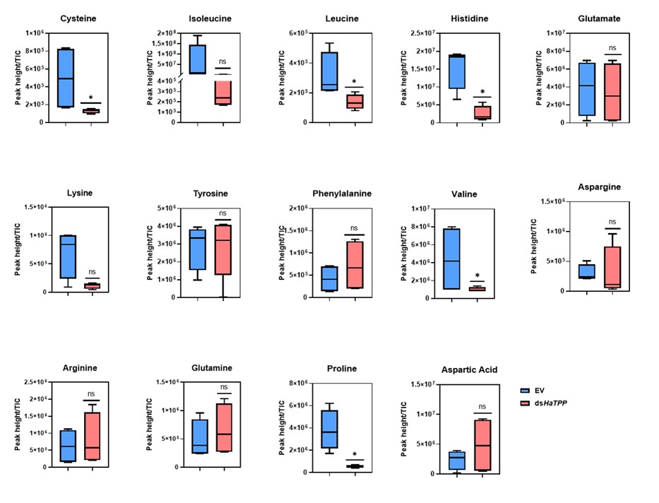
The result section of the manuscript is quite concise, to my understanding (especially the initial few sections), which misses out on mentioning details that would help readers understand the paper better. While technical details of the methods should be in the Materials and Methods section, the overall experimental strategy for the experiments performed should be explained in adequate detail in the results section itself or in figure legends. I would request authors to include more details in the results section. As an extension of the comment above, many times, abbreviations have been used without introducing them. A thorough check of the manuscript is required regarding this.
Thank you very much for pointing out this issue. We will revise the manuscript content according to these suggestions.
The Spodoptera experiments appear ad hoc and are insufficient to support conservation beyond Helicoverpa. To substantiate this claim, please add a coherent, minimal set of Spodoptera experiments and present them in a dedicated subsection. Alternatively, consider removing these data and limiting the conclusions (and title) to H. armigera.
We thank the reviewer for this helpful comment. We agree that, in this current version of the manuscript, the S. frugiperda experiments are not sufficiently systematic to support strong claims about conservation beyond H. armigera. Our primary focus in this study is indeed on H. armigera, and the addition of the S. frugiperda data was intended only as preliminary, supportive evidence rather than a central component of our conclusions. To avoid over‑interpretation and to keep the manuscript focused and coherent, we will remove all S. frugiperda data from the revised version, including the corresponding text and figures. We will also adjust the title, abstract, and conclusion to clearly state that our findings are limited to H. armigera.
In order to check the effects of E2F/Dp, a dsRNA-mediated knockdown of Dp was performed. Why was the E2F protein, a primary target of the study, not chosen as a candidate? The authors should either provide justification for this or perform the suggested experiments to come to a conclusion. I would like to point out that such experiments were performed in Drosophila.
Thank you for this thoughtful comment and the specific suggestion. We agree that directly targeting E2F would, in principle, be an informative complementary approach. In our study, however, we prioritized Dp knockdown for two main reasons. First, E2F is a large family, and E2F-Dp functions as an obligate heterodimer. Previous work in D. melanogaster has shown that depletion of Dp is sufficient to disrupt E2F-dependent transcription broadly, often with more efficient loss of complex activity than targeting individual E2F isoforms (Zappia et al., 2021; Zappia et al., 2016). Second, in our preliminary trials, we performed a dsRNA feeding assay with dsHaE2F, dsHaDp, and combined dsHaE2F plus dsHaDp. In that assay, we did not achieve silencing of E2F in dsRNA targeting HaE2F (dsHaE2F). So here, as E2F is a large family, other E2F isoforms may be compensating for the silencing effect of targeted HaE2F. However, HaE2F showed significantly reduced expression upon dsHaDp and combined dsHaE2F plus dsHaDp feeding (Figure A), whereas HaDp showed a significant reduction in its expression in all three conditions (Figure B). As we observed reduced expression of both HaE2F and HaDp upon combined feeding of dsHaE2F and dsHaDp, we further performed a rescue assay by exogenous feeding of trehalose. We observed the significant upregulation of HaE2F, HaDp, trehalose metabolic genes (HaTPS/TPP and HaTreh1), and myogenic genes (HaPrm and HaTm2) (Figure C). For these reasons, we focused on Dp silencing as a more reliable way to impair E2F/Dp complex function in H. armigera.
Author response image 2.
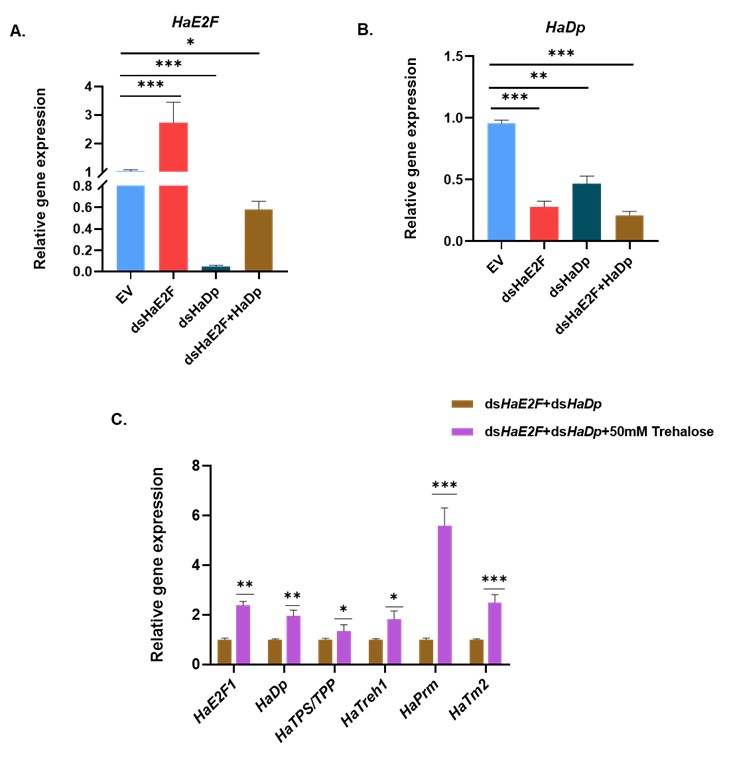
References:
(1) Zappia, M.P. and Frolov, M.V., 2016. E2F function in muscle growth is necessary and sufficient for viability in Drosophila. Nature Communications, 7(1), p.10509.
(2) Zappia, M.P., Guarner, A., Kellie-Smith, N., Rogers, A., Morris, R., Nicolay, B., Boukhali, M., Haas, W., Dyson, N.J. and Frolov, M.V., 2021. E2F/Dp inactivation in fat body cells triggers systemic metabolic changes. elife, 10, p.e67753.
Silencing of HaDp resulted in a significant decrease in HaE2F expression. I find this observation intriguing. DP is the cofactor of E2F, and they both heterodimerise and sit on the promoter of target genes to regulate them. I would request authors to revisit this result, as it contradicts the general understanding of how E2F/Dp functions in other organisms. If Dp indeed controls E2F expression, then further experiments should be conducted to come to a conclusion convincingly. Additionally, these results would need thorough discussion with citations of similar results observed for other transcription factor-cofactor complexes.
Thank you for highlighting this point and for prompting us to examine these data more carefully. Silencing HaDp leading to reduced HaE2F mRNA is indeed unexpected if one only considers the canonical view of E2F/Dp as a heterodimer that co-occupies target promoters without strongly regulating each other’s expression. However, several lines of work suggest that transcription factor-cofactor networks frequently include feedback loops in which cofactors influence the expression of their partner TFs. First, in multiple systems, transcription factors and their cofactors are known to regulate each other’s transcription, forming positive or negative feedback loops. For example, in hematopoietic cells, the transcription factor Foxp3 controls the expression of many of its own cofactors, and some of these cofactors in turn facilitate or stabilize Foxp3 expression, forming an interconnected regulatory network rather than a simple one‑way interaction (Rudra et al., 2012). Second, E2F/Dp complexes exhibit non‑canonical regulatory mechanisms and can regulate broad sets of targets, including other transcriptional regulators. Several studies show that E2F/Dp proteins not only control classical cell‑cycle genes but also participate in diverse processes such as DNA damage signaling, mitochondrial function, and differentiation (Guarner et al., 2017; Ambrus et al., 2013; Sánchez-Camargo et al., 2021). In D. melanogaster, complete loss of dDP alters the expression of direct targets E2F/DP, including dATM (Guarner et al., 2017).
All these reports indicate that the E2F-Dp complex sits at the top of multi‑layer regulatory hierarchies. Such architectures make it plausible that Dp silencing in H. armigera could modulate HaE2F expression in a non-canonical way.
References:
(1) Rudra, D., DeRoos, P., Chaudhry, A., Niec, R.E., Arvey, A., Samstein, R.M., Leslie, C., Shaffer, S.A., Goodlett, D.R. and Rudensky, A.Y., 2012. Transcription factor Foxp3 and its protein partners form a complex regulatory network. Nature immunology, 13(10), pp.1010-1019.
(2) Guarner, A., Morris, R., Korenjak, M., Boukhali, M., Zappia, M.P., Van Rechem, C., Whetstine, J.R., Ramaswamy, S., Zou, L., Frolov, M.V. and Haas, W., 2017. E2F/DP prevents cell-cycle progression in endocycling fat body cells by suppressing dATM expression. Developmental cell, 43(6), pp.689-703.
(3) Ambrus, A.M., Islam, A.B., Holmes, K.B., Moon, N.S., Lopez-Bigas, N., Benevolenskaya, E.V. and Frolov, M.V., 2013. Loss of dE2F compromises mitochondrial function. Developmental cell, 27(4), pp.438-451.
(4) Sánchez-Camargo, V.A., Romero-Rodríguez, S. and Vázquez-Ramos, J.M., 2021. Non-canonical functions of the E2F/DP pathway with emphasis in plants. Phyton, 90(2), p.307.
I consider the overall bioinformatics analysis to remain very poorly described. What is specifically lacking is clear statements about why a particular dry lab experiments were conducted.
We again thank the reviewer for advising us to give a biological context/motivation for every bioinformatics analysis performed. The bioinformatics analyses devised here, try to explain the systems-level perturbations of HaTPS/TPP silencing to explain the observed phenotype and to discover transcription factors potentially modulating the HaTPS/TPP induced gene regulatory changes.
(1) Gene set enrichment analyses:
Differential gene expression analyses of the bulk RNA sequencing data followed by qRT-PCR confirmed the transcriptional changes in myogenic genes and gene expression alterations in metabolic and cell cycle-related genes. These perturbations merely confirmed the effect induced by HaTPS/TPP silencing in obviously expected genes. We wanted to see whether using an “unbiased” system-level statistical analyses like gene set enrichment analyses (GSEA), can reveal both expected and novel biological processes that underlie HaTPS/TPP silencing. GSEA results revealed large-scale transcriptional changes in 11 enriched processes, including amino acid metabolism, energy metabolism, developmental regulatory processes, and motor protein activity. GSEA not only divulged overall transcriptionally enriched pathways but also identified the genes undergoing synchronized pathway-level transcriptional change upon HaTPS/TPP silencing.
(2) Gene regulatory network analysis:
Although GSEA uncovered potential pathway-level changes, we were also interested in identifying the gene regulatory network associated with such large-scale process-level transcriptional perturbations. Interestingly, the biological processes undergoing perturbations were also heterogeneous (e.g., motor protein activity, energy metabolism, amino acid metabolism, etc.). We hypothesized that the inference of a causal gene regulatory network associated with the genes associated with GSEA-enriched biological processes should predict core/master transcription factors that might synchronously regulate metabolic and non-metabolic processes related to HaTPS/TPP silencing, thereby providing a broad understanding of the perturbed phenotype. The gene regulatory network analysis statistically inferred an “active” gene regulatory network corresponding to the GSEA-enriched KEGG gene sets. Ranking the transcription factors (TFs) based on the number of outgoing connections (outdegree centrality) within the active gene regulatory network, E2F family TFs were identified to be top-ranking, highly connected transcription factors associated with the transcriptionally enriched processes. This suggests that E2F family TFs are central to controlling the flow of regulatory information within this network. Intriguingly, E2F has been previously implicated in muscle development in insects (Zappia et al., 2016). Further extracting the regulated targets of E2F family TFs within this network revealed the mechanistic connection with the 11 enriched processes. This GRN analysis was crucial in discovering and prioritizing E2F TFs as central transcription factors mediating HaTPS/TPP silencing effects, which was not apparent using trivial analyses like differential gene expression analysis.
As per the reviewer’s suggestions, we will add these outlined points in the text of the manuscript (Results section) to further give context and clarity to the bioinformatics analyses conducted in this study.
In my judgement, the EMSA analysis presented is technically poor in quality. It lacks positive and negative controls, does not show mutation analysis or super shifts. Also, it lacks any competition assays that are important to prove the binding beyond doubt. I am not sure why protein is not detected at all in lower concentrations. Overall, the EMSA assays need to be redone; I find the current results to be unacceptable.
Thank you for pointing out this issue. We will reperform the EMSA analysis with appropriate controls. Although the gel image was not clear, there was a light band of protein (indicated by the white square) observed in well No. 8, where we used 8 μg of E2F protein and 75 ng of HaTPS/TPP promoter, upon gel stained with SYPRO Ruby protein stain, suggesting weak HaTPS/TPP-E2F complex formation.
GSEA studies clearly indicate enrichment of the amino acid synthesis gene in TPP knockdown samples. This supports the plausible theory that a lack of Trehalose means a lack of enough nutrients, therefore less of that is converted to amino acids, and therefore muscle development is compromised. Yet the authors make no effort to measure amino acid levels. While nutrients can be sensed through signalling pathways leading to shut shutdown of myogenic genes, a simple and direct correlation between less raw material and deformed muscle might also be possible.
We quantified amino acid levels as per the suggestion, and we observed differential levels of amino acids upon trehalose metabolism perturbation.
However, we observed that insect were failed to rescue when fed a control chickpea-based artificial diet that contained nutrients required for normal growth and development. Based on this observation, we conclude that trehalose deficiency is the only possible cause for the defect in muscle development.
The authors are encouraged to stick to one color palette while demonstrating sequencing results. Choosing a different color palette for representing results from the same sequencing analysis confuses readers.
Thank you for the comment. We will revise the color palette as per the suggestion.
Expression of genes, as understood from sequencing analysis in Figure 1D, Figure 2F, and Figure 3D, appears to be binary in nature. This result is extremely surprising given that the qRT-PCR of these genes have revealed a checker and graded expression.
Thank you for pointing out this issue. We will revise the scale range for these figures to get more insights about gene expression levels and include figures as per the suggestion.
In several graphs, non-significant results have been interpreted as significant in the results section. In a few other cases, the reported changes are minimal, and the statistical support is unclear; please recheck the analyses and include exact statistics. In the results section, fold changes observed should be discussed, as well as the statistical significance of the observed change.
We will revise the analyses and include exact statistics as per the suggestion.
Finally, I would add that trehalose metabolism regulates cell cycle genes, and muscle development genes establish correlation and causation. The authors should ensure that any comments they make are backed by evidence.
We thank the reviewer for this insightful comment. Although direct evidence in insects is currently lacking, multiple independent studies in yeast, plants and mammalian systems support a regulatory link between trehalose metabolism and the cell cycle. In budding yeast Saccharomyces cerevisiae, neutral Treh (Nth1) is directly phosphorylated and activated by the major cyclin‑dependent kinase Cdk1 at G1/S, routing stored trehalose into glycolysis to fuel DNA replication and mitosis (Ewald et al., 2016). CDK‑dependent regulation of trehalase activity has also been reported in plants, where CDC28‑mediated phosphorylation channels glucose into biosynthetic pathways necessary for cell proliferation (Lara-núñez et al., 2025). Furthermore, budding yeast cells accumulate trehalose and glycogen upon entry into quiescence and subsequently mobilize these stores to generate a metabolic “finishing kick” that supports re‑entry into the cell cycle (Silljé et al., 1999; Shi et al., 2010). Exogenous trehalose that perturbs the trehalose cycle impairs glycolysis, reduces ATP, and delays cell cycle progression in S. cerevisiae, highlighting a dose‑ and context‑dependent control of growth versus arrest (Zhang, Zhang and Li, 2020). In mammalian systems, trehalose similarly modulates proliferation-differentiation decisions. In rat airway smooth muscle cells, low trehalose concentrations promote autophagy, whereas higher doses induce S/G2–M arrest, downregulate Cyclin A1/B1, and trigger apoptosis, indicating a shift from controlled growth to cell elimination at higher exposure (Xiao et al., 2021). In human iPSC‑derived neural stem/progenitor cells, low‑dose trehalose enhances neuronal differentiation and VEGF secretion, while higher doses are cytotoxic, again highlighting a tunable impact on cell‑fate outcomes (Roose et al., 2025). In wheat, exogenous trehalose under heat stress reduces growth, lowers auxin, gibberellin, abscisic acid and cytokinin levels, and represses CycD2 and CDC2 expression, suggesting that trehalose signalling integrates with hormone pathways and core cell‑cycle regulators to restrain proliferation during stress (Luo, Liu, and Li, 2021). Together, these studies showed the importance of trehalose metabolism in cell‑cycle regulation to decide whether cells and tissues proliferate, differentiate, or remain quiescent.
With respect to muscle development, previous work has implicated glycolytic metabolism in myogenesis and muscle growth. Tixier et al. (2013) showed that loss of key glycolytic genes results in abnormally thin muscles, while Bawa et al. (2020) demonstrated that loss of TRIM32 decreases glycolytic flux and reduces muscle tissue size. These findings indicate that carbohydrate and energy metabolism pathways are important determinants of muscle structure and growth. However, there are no previous studies about the role of trehalose metabolism in muscle development, other than as an energy source, so here we specifically set out to establish the involvement of trehalose metabolism in muscle development.
References:
(1) Ewald, J.C. et al. (2016) “The yeast cyclin-dependent kinase routes carbon fluxes to fuel cell cycle progression,” Molecular cell, 62(4), pp. 532–545.
(2) Lara-núñez, A. et al. (2025) “The Cyclin-Dependent Kinase activity modulates the central carbon metabolism in maize during germination,” (January), pp. 1–16.
(3) Silljé, H.H.W. et al. (1999) “Function of trehalose and glycogen in cell cycle progression and cell viability in Saccharomyces cerevisiae,” Journal of bacteriology, 181(2), pp. 396–400.
(4) Shi, L. et al. (2010) “Trehalose Is a Key Determinant of the Quiescent Metabolic State That Fuels Cell Cycle Progression upon Return to Growth,” 21, pp. 1982–1990.
(5) Zhang, X., Zhang, Y. and Li, H. (2020) “Regulation of trehalose, a typical stress protectant, on central metabolisms, cell growth and division of Saccharomyces cerevisiae CEN. PK113-7D,” Food Microbiology, 89, p. 103459.
(6) Xiao, B. et al. (2021) “Trehalose inhibits proliferation while activates apoptosis and autophagy in rat airway smooth muscle cells,” Acta Histochemica, 123(8), p. 151810.
(7) Roose, S.K. et al. (2025) “Trehalose enhances neuronal differentiation with VEGF secretion in human iPSC-derived neural stem / progenitor cells,” Regenerative Therapy, 30, pp. 268–277.
(8) Luo, Y., Liu, X. and Li, W. (2021) “Exogenously-supplied trehalose inhibits the growth of wheat seedlings under high temperature by affecting plant hormone levels and cell cycle processes,” Plant Signaling & Behavior, 16(6).
(9) Tixier, V., Bataillé, L., Etard, C., Jagla, T., Weger, M., DaPonte, J.P., Strähle, U., Dickmeis, T. and Jagla, K., 2013. Glycolysis supports embryonic muscle growth by promoting myoblast fusion. Proceedings of the National Academy of Sciences, 110(47), pp.18982-18987.
(10) Bawa, S., Brooks, D.S., Neville, K.E., Tipping, M., Sagar, M.A., Kollhoff, J.A., Chawla, G., Geisbrecht, B.V., Tennessen, J.M., Eliceiri, K.W. and Geisbrecht, E.R., 2020. Drosophila TRIM32 cooperates with glycolytic enzymes to promote cell growth. elife, 9, p.e52358.
Finally, we appreciate the meticulous review of this manuscript and constructive comments. We will perform the recommended experiments, data analysis, and revise the manuscript accordingly.
RRID:SCR_002865
DOI: 10.1038/s41420-025-02886-y
Resource: SPSS (RRID:SCR_002865)
Curator: @dhovakimyan1
SciCrunch record: RRID:SCR_002865
RRID: AB_2813911
DOI: 10.1007/s12020-025-04499-y
Resource: (Abbott Cat# 7K72-25, RRID:AB_2813911)
Curator: @dhovakimyan1
SciCrunch record: RRID:AB_2813911
AB_2813909
DOI: 10.1007/s12020-025-04499-y
Resource: (Abbott Cat# 2P40-25, RRID:AB_2813909)
Curator: @scibot
SciCrunch record: RRID:AB_2813909
RRID:AB_2924942
DOI: 10.1007/s12020-025-04499-y
Resource: (Abbott Cat# 5P02, RRID:AB_2924942)
Curator: @scibot
SciCrunch record: RRID:AB_2924942
RRID:AB_2895254
DOI: 10.1007/s12020-025-04499-y
Resource: (Abbott Cat# 2P13, RRID:AB_2895254)
Curator: @scibot
SciCrunch record: RRID:AB_2895254
RRID:AB_2813910
DOI: 10.1007/s12020-025-04499-y
Resource: (Abbott Cat# 7K75-25, RRID:AB_2813910)
Curator: @scibot
SciCrunch record: RRID:AB_2813910
RRID:AB_476744
DOI: 10.1186/s13062-025-00722-y
Resource: (Sigma-Aldrich Cat# A5441, RRID:AB_476744)
Curator: @scibot
SciCrunch record: RRID:AB_476744
RRID:AB_3265513
DOI: 10.1186/s13062-025-00722-y
Resource: Cell Signaling Technology Cat# 32683, RRID:AB_3265513
Curator: @scibot
SciCrunch record: RRID:AB_3265513
RRID:AB_11125142
DOI: 10.1186/s13062-025-00722-y
Resource: (Bio-Rad Cat# 170-6515, RRID:AB_11125142)
Curator: @scibot
SciCrunch record: RRID:AB_11125142
RRID:AB_2749902
DOI: 10.1186/s13062-025-00722-y
Resource: (BioLegend Cat# 905403, RRID:AB_2749902)
Curator: @scibot
SciCrunch record: RRID:AB_2749902
RRID:AB_11125547
DOI: 10.1186/s13062-025-00722-y
Resource: (Bio-Rad Cat# 170-6516, RRID:AB_11125547)
Curator: @scibot
SciCrunch record: RRID:AB_11125547
RRID:CVCL_0037
DOI: 10.1186/s13062-025-00722-y
Resource: (RCB Cat# RCB1872, RRID:CVCL_0037)
Curator: @scibot
SciCrunch record: RRID:CVCL_0037
RRID:CVCL_S877
DOI: 10.1186/s13062-025-00722-y
Resource: (RRID:CVCL_S877)
Curator: @scibot
SciCrunch record: RRID:CVCL_S877
AB_2281408
DOI: 10.1016/j.isci.2026.114906
Resource: (BioLegend Cat# 116222, RRID:AB_2281408)
Curator: @scibot
SciCrunch record: RRID:AB_2281408
RRID:AB_3675250
DOI: 10.1016/j.celrep.2026.116952
Resource: None
Curator: @scibot
SciCrunch record: RRID:AB_3675250
las características que debe cumplir un objetivo forman el acrónimo SMART:• Específico• Medible• Alcanzable• Relevante• Temporal
SMART asegura que los objetivos sean claros y alcanzables. Lo que evita plantear metas ambiguas o dificiles de cumplir. La medición y temporalidad permiten evaluar si el estudio logró lo que se propuso.
De la idea de investigación nace la pregunta central de investigación y las preguntasauxiliares de investigación que guiarán el proceso de investigación.
Las preguntas de investigación son demasiado útiles y sirven como una guia metodológica. Ya que estas orientan todo el proceso y evitan desviaciones.
La descripción del problema:
El enunciado hace que se pueda contextualizar el problema de una manera profunda. No solo es mencionar el problema, sino que se deben analizar sus causas y efectos. Lo que ayuda a comprender su impacto real.
Refleja el área temática a investigar• Responde los aspectos deo Especificidad: ¿Qué se investiga?o Espacialidad ¿Dónde se realiza?o Temporalidad ¿Cuándo se lleva a cabo?
El título es una síntesis estructurada del estudio. Debe indicar qué se investiga, dónde y cuándo. Lo que permite delimitar el estudio y evitar ambigüedades, esto al final garantiza precisión desde el inicio.
La justificación explica el porqué de la investigación: por qué elproyecto es importante y necesario.
No se investiga por curiosidad únicamente, sino que también para aportar soluciones, conocimiento o beneficios prácticos. Evaluar lo que es su conveniencia y relevancia fortalece el valor académico del proyecto.
Un problema planteado de forma correcta está parcialmente resuelto, ya que, a mayorexactitud, hay más posibilidades de obtener una solución satisfactoria.
Esta idea es clave porque nos muestra que la claridad en la formulación del problema es muy importante y determina la calidad de toda la investigación. Si el problema no es exacto, el estudio perderá dirección. Por lo que hay que definirlo correctamente para aumentar las probabilidades de obtener resultados válidos y útiles.
ThisURL returnsa “404 Notfound” errorfor us. Pleasedouble-check
Looking at the internet archives, this URL was moved elsewhere. Please use this new citation:
Shah Y, et al. Safety and efficacy of Impella RP support for acute right ventricular failure complicated by cardiogenic shock: post market approval sub-analysis of the CVAD registry. J Card Fail. 2024;30(1):269.
def shape(piece_grid): cells = [] for y, row in enumerate(piece_grid): for x, ch in enumerate(row): if ch == "x": cells.append([x, y]) return cells
Ett alternativ utan append, men inte helt glasklart om det är tydligare än for-loopen.
med comprehensions i två nivåer:
def shape(piece_grid):
    return [
        [x, y]
        for y, row in enumerate(piece_grid)
        for x, ch in enumerate(row)
        if ch == "x"
    ]
y released five EPs, two single
fsdfasdfasd
f o r e i g n e r e n d e a v o u r i n g t o u n d e r s t a n d t h e t r u ec h a r a c t e r of t h e B r i t i s h E m p i r e by t h e a i d of t h i sf p r m u l a a l o n e might be tempted, t o t h i n k t h a t i t wasd e v i s e d r a t h e r t o make m u t u a l i n t e r f e r e n c e i m p o s s i b l et h a n t o make m u t u a l c o o p e r a t i o n e a s y
This paragraph explains that outsiders might see this system as preventing interference rather than encouraging cooperation. Because each Dominion is fully independent, there is no central authority forcing unity. The structure prioritizes sovereignty and equality, even if that makes cooperation less automatic.
They a r e autonomous c o m m u n i t i e sw i t h i n t h e B r i t i s h J ^ P j £ e m e q u a l i n s t a t u s , i n no ways u b o r d i n a t e one t o a n o t h e r i n a n y a s p e c t of t h e i r d o m e s t i cor e x t e r n a l a f f a i r s , t h o u g h u n i t e d by a commona l l e g i a n c e t o t h e Crown,, and f r e e l y a s s o c i a t e d a s membersof t h e B r i t i s h Commonwealth of E a t i o n s
The statement that the Dominions are “autonomous communities… equal in status” shows that Britain no longer had authority over them. They controlled their own domestic and foreign affairs and were not subordinate to one another. However, they remained united by a shared allegiance to the Crown. This marks the shift from empire to a voluntary Commonwealth of equal nations.
y, however, we issued aclarification, accompanied by a lengthy editors’ note: By saying that protecting slavery was “oneof the primary reasons,” Nikole did not mean to imply that it was a primary reason for every oneof the colonists, who were, after all, a geographically and culturally diverse lot with varyinginterests; rather, she meant that one of the primary reasons driving some of them, particularlythose from the Southern colonies, was the protection of slavery from British meddling. Weclarified this by adding “some of” to Nikole’s original sentence
Shows that the Times responded to criticism but stood by the broader argument about slavery and the Revolution.
on: El Reino de Italia, Reino Unido de Gran Bretaña e Irlanda, Francia y el Imperio ruso.
Kingdoms?
Author response:
The following is the authors’ response to the original reviews.
Reviewer #1:
Summary:
In their study, the authors investigated the F. graminearum homologue of the Drosophila Misato-Like Protein DML1 for a function in secondary metabolism and sensitivity to fungicides.
Strengths:
Generally, the topic of the study is interesting and timely, and the manuscript is well written, albeit in some cases, details on methods or controls are missing.
Weaknesses:
However, a major problem I see is with the core result of the study, the decrease in the DON content associated with the deletion of FgDML1. Although some growth data are shown in Figure 6, indicating a severe growth defect, the DON production presented in Figure 3 is not related to biomass. Also, the method and conditions for measuring DON are not described. Consequently, it could well be concluded that the decreased amount of DON detected is simply due to decreased growth, and the specific DON production of the mutant remains more or less the same.
To alleviate this concern, it is crucial to show the details on the DON measurement and growth conditions and to relate the biomass formation under the same conditions to the DON amount detected. Only then can a conclusion as to an altered production in the mutant strains be drawn.
We appreciate it very much that you spent much time on my paper and give me good suggestions, we tried our best to revise the manuscript. I have revised my manuscript according to your suggestions. The point to point responds to the reviewer’s comments are listed as following. Our method for DON quantification was based on the amount per unit of mycelium. After obtaining the absorbance value from the ELISA reaction, the concentration of DON was calculated according to a standard curve and a formula, then divided by the dry weight of the mycelium to obtain the DON content per unit of mycelium, with the results finally expressed in µg/g.
(1) Line 139f
... FgDML1 is a critical positive regulator of virulence ....
Clearly, the deletion of FgDML1 impacts virulence, but it is too much of a general effect to say it is a regulator. DML1 acts high up in the cascade, impacting numerous processes, one of which is virulence. Generally, it has to be considered that deletion of DML1 causes a severe growth defect, which in turn is likely to lead to a plethora of effects. Besides discussing this fact, please also revise the manuscript to avoid references to "direct effects" or "regulator".
Thank you very much for your advice. Our method for determining the amount of DON is based on the amount of mycelium per unit. After obtaining the absorbance value through Elisa reaction, we calculate the concentration of DON toxin according to the established standard curve and formula. Then, we divide it by the dry weight of mycelium to obtain the DON toxin content per unit mycelium, and finally present the results in µg/g. In summary, we conclude that the decrease in DON production by ΔFgDML is not due to slower hyphal growth, but rather a decrease in the ability of unit hyphae to produce DON toxins compared to the wild type. Given the decrease in DON toxin synthesis caused by FgDML1 deficiency, we believe that using a regulator is reasonable.
(2) Line 143
Please define "toxin-producing conditions".
Thank you very much for your advice. We have accurately defined the conditions for toxin-producing conditions in the manuscript' toxin-inducing conditions '(28°C, 145 ×g, 7 days incubation)' (in L163-164)
(3) Line 149
A brief intro on toxisomes should be provided in the introduction to better integrate this into the manuscript's results.
Thank you very much for your advice. We have added corresponding content about toxin producing bodies in the introduction section 'The biosynthesis of DON entails a reorganization of the endoplasmic reticulum into a specialized compartment termed the "toxisome" (Tang et al., 2018). The assembly of the toxisome coincides with the aggregation of key biosynthetic enzymes, which in turn enhances the efficiency of DON production. Concurrently, this compartmentalization serves as a self-defense mechanism, protecting the fungus from the autotoxicity of TRI pathway intermediates (Boenisch et al., 2017). The proteins TRI1, TRI4, TRI14, and Hmr1 are confirmed constituents of this structure(Kistler and Broz, 2015; Menke et al., 2013).' (in L86-93)
(4) Line 153
DON production decreases by about 80 %, but not to 0. Consequently, DML1 is important, but NOT essential for DON production.
Thank you very much for your advice. We have made changes to the wording of the corresponding sections based on your suggestions. 'FgDML1 is essential for the biosynthesis of the DON toxin. '(in L161)
(5) Line 168ff
Please provide a reference for FgDnm1 being critical for mitochondrial fission and state whether such an interaction has been shown in other organisms.
Thank you very much for your advice. We have made changes to the wording of the corresponding sections based on your suggestions. 'FgDnm1 is a key dynamin-related protein mediating mitochondrial fission(Griffin et al., 2005; Kang et al., 2023), suggesting that FgDML1 may form a complex with FgDnm1 to regulate mitochondrial fission and fusion processes. To our knowledge, this is the first report documenting an interaction between DML1 and Dnm in any fungal species, including model organisms such as S. cerevisiae. This novel finding provides new insights into the molecular mechanisms underlying mitochondrial dynamics in filamentous fungi. '(in L277-283)
(6) Line 178
Please specify whether Complex III activity was related to biomass and provide a p-value or standard deviation for the value.
Thank you very much for your question. The activity determination of complex III was completed using a complex III enzyme activity kit (Solarbio, Beijing, China) (Li, et al 2022; Wang, et al 2022). Take 0.1 g of standardized mycelium as the sample for the experiment. Given that the mycelium has been homogenized, we believe that there is no necessary correlation between the activity and biomass of complex III. And we also refined the specific measurement steps in the article. ' Briefly, 0.1 g of mycelia was homogenized with 1 mL of extraction buffer in an ice bath. The homogenate was centrifuged at 600 ×g for 10 min at 4°C. The resulting supernatant was then subjected to a second centrifugation at 11,100 ×g for 10 min at 4°C. The pellet was resuspended in 200 μL of extraction buffer and disrupted by ultrasonication (200 W, 5 s pulses with 10 s intervals, 15 cycles). Complex III enzyme activity was finally measured by adding the working solution as per the manufacturer's protocol. Each treatment group contains three biological replicates and three technical replicates. '(in L511-517)
Li C, et al. Amino acid catabolism regulates hematopoietic stem cell proteostasis via a GCN2-eIF2 axis. Cell Stem Cell. 2022 Jul 7; 29(7):1119-1134.e7. doi: 10.1016/j.stem.2022.06.004. PMID: 35803229.
Wang K, et al. Locally organised and activated Fth1hi neutrophils aggravate inflammation of acute lung injury in an IL-10-dependent manner. Nat Commun. 2022 Dec 13;13(1):7703. doi: 10.1038/s41467-022-35492-y. PMID: 36513690; PMCID: PMC9745290
(7) Line 185
Albeit this headline is a reasonable hypothesis, you actually did not show that the conformation is altered. Please reword accordingly.
Please also add references for cyazofamid acting on the QI site versus other fungicides acting on the QO site.
Thank you very much for your advice. We have made changes to the wording of the corresponding sections based on your suggestions. 'Overexpression of FgQCR2, FgQCR8, and FgQCR9 may alters the conformation of the QI site, resulting in reduced sensitivity to cyazofamid. '(in L212-213). For fungicides targeting Qi and QO sites, we have added corresponding descriptions in the respective sections 'Numerous fungicides have been developed to inhibit the Qo site (e.g., pyraclostrobin, azoxystrobin)(Nuwamanya et al., 2022; Peng et al., 2022) and the Qi site (e.g., cyazofamid)(Mitani et al., 2001) of the cytochrome bc1 complex. '(in L327-329)
(8) Line 200
This section on growth should be moved up right after introducing the mutant strain.
Thank you very much for your advice. We have advanced the part of nutritional growth and sexual asexual development before DON toxin to promote better reading and understanding. We arranged the sequence in the previous way to emphasize the new discovery between mitochondria and DON toxin. We found a significant decrease in DON toxin in ΔFgDML1, defects in the formation of toxin producing bodies, and downregulation of FgTRis at both the gene and protein levels. In summary, we believe that the absence of FgDML1 does indeed lead to a decrease in the content of DON toxin, and FgDML1 plays a regulatory role in the synthesis of DON toxin. In addition, our measurements of DON toxin, acetyl CoA, ATP and other indicators are all based on the amount per unit hyphae, excluding differences caused by hyphal biomass or growth. We have further refined the materials and methods to facilitate better reading and understanding.
(9) Line 203
"... significantly reduced growth rates ..."
This is not what was measured here. Figure 6A shows a plate assay that can be used to assess hyphal extension. In the figure, it is also visible that the mycelium of the deletion mutant is much denser, maybe due to increased hyphal branching. Please reword.
Additionally, it is important to include a biomass measurement here under the conditions used for DON assessment. Hyphal extension measurements cannot be used instead of biomass.
Thank you very much for your advice. We have made changes to the wording of the corresponding sections based on your suggestions. 'The ΔFgDML1 strain displayed a distinct growth phenotype characterized by retardation in radial growth and the formation of more compact, denser hyphal networks on all tested media compared to the PH-1 and ΔFgDML-C strains. '(in L136-138).
(10) Line 217
Please include information on how long the cultures were monitored. Given the very slow growth of the mutant, perithecia formation may be considerably delayed beyond 14 days.
Thank you very much for your advice. Based on your suggestion, we have extended the incubation time for sexual reproduction to 21 days to more accurately evaluate its sexual reproduction ability. Our results show that even after 21 days, Δ FgDML1 still cannot produce ascospores and ascospores, which proves that the absence of FgDML1 does indeed cause sexual reproduction defects in F. graminearum.
Author response image 1.
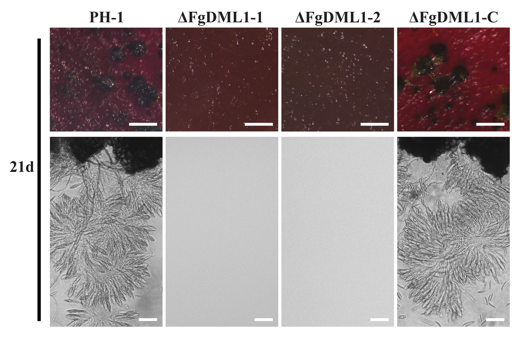
Discussion
(11) Please mention your summary Figure 8 early on in the discussion, and explain conclusions with this figure in mind. Please avoid repetition of the results section as much as possible.
Also, please state clearly what was already known from previous research and is in agreement with your results, and what is new (in fungi or generally).
Thank you very much for your advice. Based on your suggestion, we mentioned Fig8 earlier in the first half of the discussion and provided guidance for the following text. We also conducted a more comprehensive discussion by analyzing our research results and comparing them with previous studies. 'Our study defines a novel mechanism through which FgDML1 governs mitochondrial homeostasis. We demonstrate that FgDML1 directly interacts with the key mitochondrial fission regulator FgDnm1 and positively modulates cellular bioenergetic metabolism, as evidenced by elevated ATP and acetyl-CoA levels (Fig. 8). '(in L250-253). 'The Misato/DML1 protein family is evolutionarily conserved from yeast to humans and plays a critical role in mitochondrial regulation. In S. cerevisiae, DML1 is an essential gene; its deletion is lethal, while its overexpression results in fragmented mitochondrial networks and aberrant cellular morphology, underscoring its necessity for normal mitochondrial function (Gurvitz et al., 2002). Similarly, in Homo sapiens, the homolog Misato localizes to the mitochondrial outer membrane, and both its depletion and overexpression are sufficient to disrupt mitochondrial morphology and distribution (Kimura and Okano, 2007). '(in L241-244).
(12) Line 262ff
Please specify if this interaction was shown previously in other organisms and provide references.
Thank you very much for your advice. We have clearly stated in the corresponding section that the interaction between FgDML and FgDnm is the first reported, and to our knowledge, no relevant reports have been found in other species so far. ' Notably, FgDML1 was found to interact with FgDnm1 (Fig. 5E), FgDnm1 is a key dynamin-related protein mediating mitochondrial fission(Griffin et al., 2005; Kang et al., 2023), suggesting that FgDML1 may form a complex with FgDnm1 to regulate mitochondrial fission and fusion processes. To our knowledge, this is the first report documenting an interaction between DML1 and Dnm in any fungal species, including model organisms such as S. cerevisiae. This novel finding provides new insights into the molecular mechanisms underlying mitochondrial dynamics in filamentous fungi. '(in L276-283)
(13) Line 287ff
There is no result that would justify this speculation. Please remove.
Thank you very much for your advice. We have modified the corresponding wording in the corresponding section. 'In conclusion, our findings suggest that the overexpression of assembly factors FgQCR2, FgQCR7, and FgQCR8 in ΔFgDML1 potentially modifies the conformation of the Qi site, which specifically modulates the sensitivity of F. graminearum to cyazofamid. '(in L352-355)
Materials and methods
(14) A table with all primer sequences used in the study and their purpose is missing. For every experiment, the number of technical and biological replicates needs to be stated.
Thank you very much for your advice. We have presented all the primers used in this study in Supplementary Table 1 (in Table S1) .We added the number of technical and biological replicates in the material and method descriptions for each experiment. 'For each sample, a total of 200 conidia were counted. The experiment included three biological replicates with three technical replicates each.'(in L434-436). 'Each treatment group contains three biological replicates. '(in L444-445). 'Each treatment group contains three biological replicates and three technical replicates. ' (in L463-464). 'Each treatment group contains three biological replicates and three technical replicates. '(in L474-475). 'Each treatment group contains three biological replicates. '(in L483). 'Each treatment group contains three biological replicates and three technical replicates.'(in L501-502). 'Each treatment group contains three biological replicates and three technical replicates. '(in L516-517). 'The experiment was independently repeated three times. '(in L533-534).
(15) Line 369ff
Please provide final concentrations used for assays here.
Thank you very much for your advice. The final concentration has been displayed in the Figure (in Fig6. A, B) (in Fig. S3). And we have provided supplementary Table 2 to reflect the concentration in a more intuitive way.(in Table. S2)
(16) Line 383
Please provide a reference or data on the use of F2du for transformant selection and explain the abbreviation.
Thank you very much for your advice. Based on your suggestion, we have provided the full name and references of F2du. 'Transformants were selected on PDA plates containing either 100 μg/mL Hygromycin B (Yeasen, Shanghai, China) or 0.2 μmol/mL 5-Fluorouracil 2'-deoxyriboside (F2du) (Solarbio, Beijing, China)(Zhao et al., 2022). '(in L405-407).
(17) Line 407
Please provide a reference for the method and at least a brief description.
Thank you very much for your advice. Based on your suggestion, we have added references and provided a brief introduction to the method. 'As previously described (Tang et al., 2020; Wang et al., 2025), Specifically, coleoptiles were inoculated with conidial suspensions and incubated for 14 days, while leaves were inoculated with fresh mycelial plugs and incubated for 5 days, followed by observation and quantification of disease symptoms. DON toxin was measured using a Wise Science ELISA-based kit (Wise Science, Jiangsu, China) (Li et al., 2019; Zheng et al., 2018). '(in L466-471)
(18) Line 414ff
Also, here, the amount of biomass has to be considered for the measurement to be able to distinguish if actually less of the compounds were produced or if the effect seen was merely due to an altered amount of biomass present.
Thank you very much for your advice. We believe that biomass is not within the scope of our measurement indicators, as we have measured and calculated based on unit hyphae. Therefore, we have ruled out experimental bias caused by a decrease in biomass.
RNA and RT-qPCR
(19) Line 461
When the strains were transferred to AEA medium, was the biomass measured, at least wet weight, and in which culture volume was it done? It makes a big difference if the amount of (wet) biomass dilutes a small amount of fungicide-containing culture or if biomass is added in at least roughly equal amounts in sufficient growth medium to ensure equal conditions.
Thank you very much for your question. Our sample processing controlled the wet weight of the samples before dosing, ensuring that the wet weight of the mycelium obtained from each sample before dosing was 0.2g. The mycelium was obtained through AEA with a volume of 100mL. This ensured consistency in the initial biomass between groups before dosing, and also ensured the accuracy of the drug concentration.
(20) Line 466
Please provide the name and supplier of the kit.
Thank you very much for your advice. We have added corresponding content in the corresponding location. 'Mycelium was collected and total RNA was extracted following the instructions provided by the Total RNA Extraction Kit (Tiangen, Beijing, China).' (in L523-524).
(21) All primer sequences must be provided in a table.
Thank you very much for your advice. We have presented all the primers used in this study in Supplementary Table 1. (in Table S1).
(22) For RT qPCR it is essential to check the RNA quality to be sure that the obtained results are not artifacts due to varying quality, which may exceed differences. Please state how quality control was done and which threshold was applied for high-quality RNA to be used in RTqPCR (like RIN factor, etc).
Thank you very much for your question. We performed stringent quality control on the extracted total RNA. First, a micro-spectrophotometer was used to measure RNA concentration and purity, confirming that the A260/A280 ratio was between 1.8 and 2.0 and the A260/A230 ratio was greater than 2.0, indicating good RNA purity without significant protein or organic solvent contamination.Subsequently, verification by agarose gel electrophoresis revealed distinct 28S and 18S rRNA bands, demonstrating good RNA integrity and absence of degradation.
Author response image 2.
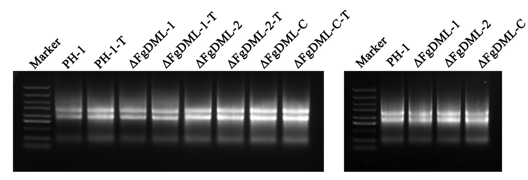
(B): Minor Comments:
(1) Please increase the font size of the labels and annotations of the figures; it is hard to read as it is now.
Thank you very much for your advice. We have increased the size of annotations or numerical labels in the corresponding images for better reading.
(2) Throughout the manuscript: Please check that all abbreviations are explained at first use.
Thank you very much for your advice. We have checked the entire text to ensure that abbreviations have their full names when they first appear.
(3) I do hope that the authors can clarify all concerns and provide an amended manuscript of this interesting story.
Thank you very much for your advice. Sincerely thank you for your suggestions and questions, which have been very helpful to us.
Reviewer #2:
The manuscript entitled "Mitochondrial Protein FgDML1 Regulates DON Toxin Biosynthesis and Cyazofamid Sensitivity in Fusarium graminearum by affecting mitochondrial homeostasis" identified the regulatory effect of FgDML1 in DON toxin biosynthesis and sensitivity of Fusarium graminearum to cyazofamid. The manuscript provides a theoretical framework for understanding the regulatory mechanisms of DON toxin biosynthesis in F. graminearum and identifies potential molecular targets for Fusarium head blight control. The paper is innovative, but there are issues in the writing that need to be addressed and corrected.
We appreciate it very much that you spent much time on my paper and give me good suggestions, we tried our best to revise the manuscript. I have revised my manuscript according to your suggestions with red words. In the response comments, to highlight the specific positions of the revised parts in the manuscript with red line number. The point to point responds to the reviewer’s comments are listed as following.
Weaknesses:
(1) The authors speculate that cyazofamid treatment caused upregulation of the assembly factors, leading to a change in the conformation of the Qi protein, thus restoring the enzyme activity of complex III. But no speculation was given in the discussion as to why this would lead to the upregulation of assembly factors, and how the upregulation of assembly factors would change the protein conformation, and is there any literature reporting a similar phenomenon? I would suggest adding this to the discussion.
Thank you very much for your advice. Based on your suggestion, we have added content related to the assembly factor of complex III in the discussion section and made modifications to the corresponding wording. 'Previous studies have reported that mutations in the Complex III assembly factors TTC19, UQCC2, and UQCC3 impair the assembly and activity of Complex III (Feichtinger et al., 2017; Wanschers et al., 2014). '(in L345-347). 'In conclusion, our findings suggest that the overexpression of assembly factors FgQCR2, FgQCR7, and FgQCR8 in ΔFgDML1 potentially modifies the conformation of the Qi site, which specifically modulates the sensitivity of F. graminearum to cyazofamid. '(in L352-355).
(2) Would increased sensitivity of the mutant to cell wall stress be responsible for the excessive curvature of the mycelium?
Thank you very much for your question. We believe that the sensitivity of ΔFgDML1 to osmotic stress is reduced, which may not be related to hyphal bending, as shown in the Author response image 3. During the conidia stage, ΔFgDML1 cannot germinate in YEPD, while the application of 1M Sorbitol promotes its germination. But it is caused by internal unknown mechanisms, which is also the focus of our future research.
Author response image 3.
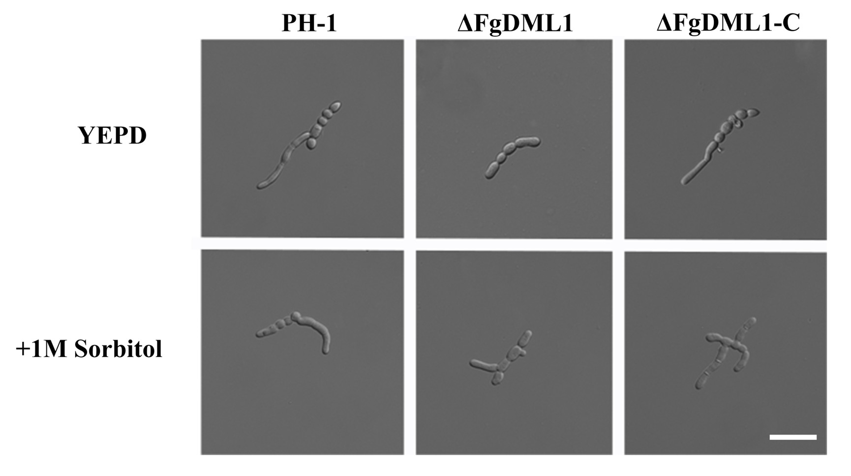
(3) The vertical coordinates of Figure 7B need to be modified with positive inhibition rates for the mutants.
Thank you very much for your advice. The display in Figure 7B truly reflects its inhibition rate. In the Δ FgDML1 mutant, when subjected to osmotic stress treatment, the inhibition rate becomes negative, indicating that the colony growth is greater than that of the CK. Therefore, the negative inhibition rate is shown in Figure 7B.
(1) In Figure 1B, Figure 3C, and Figure 6C, the scale below the picture is not clear. In Figure 5D, the histogram is unclear, and it is recommended to redraw the graph.
Thank you very much for your advice. The issue with the above images may be due to Word compression. We have changed the settings and enlarged the images as much as possible to better display them.
(2) The full Latin name of the strain should be used in the title of figures and tables.
Thank you very much for your advice. Based on your suggestion, we have used the full names of the strains appearing in the title of figures and tables.
(3) Proteins in line 117 should be abbreviated.
Thank you very much for your advice. Based on your suggestion, we have abbreviated the corresponding positions. 'The DML1 protein from S. cerevisiae was used as a query for a BLAST search against the Fusarium genome database, resulting in the identification of the putative DML1 gene FgDML1 (FGSG_05390) in F. graminearum. '(in L118-120).
(4) The sentence in lines 187-189, which is supposed to introduce why the test is sensitive to the three drugs, is currently illogical.
Thank you very much for your advice. Based on your suggestion, we have made modifications to the corresponding sections. 'Since Complex III is involved in the action of both cyazofamid (targeting the QI site) and pyraclostrobin (targeting the QO site), the sensitivity of ΔFgDML1 to cyazofamid and pyraclostrobin was investigated. ' (in L214-216).
(5) The expression of FgQCR2, FgQCR7, and FgQCR8 was significantly upregulated in ΔFgDML1 at transcription levels. Do FgQCR2, FgQCR8, and FgQCR9 show upregulated expression at the protein level?
Thank you very much for your question. Based on your suggestion, we evaluated the protein expression levels of FgQCR2, FgQCR7, and FgQCR8 in PH-1 and ΔFgDML1, and we found that the protein expression levels of FgQCR2, FgQCR7, and FgQCR8 in ΔFgDML1 were higher than those in PH-1. (in Fig. 6F).
(6) In Figure 7B, it is recommended to adjust the position of the horizontal axis labels in the histogram.
Thank you very much for your advice. Based on your suggestion, we have made modifications to the corresponding sections.(in Fig. 7B)
(7) There are numerous errors in the writing of gene names in the text. Please check the full text and change the writing of gene names and mutant names to italic.
Thank you very much for your advice. We have checked the entire text to ensure that all genes have been italicized.
(8) All acronyms should be spelled out in figure and table captions. e.g., F. graminearum.
Thank you very much for your advice. Based on your suggestion, we have used the full names of the strains appearing in the title of figures and tables.
(9) In line 492, P should be lowercase and italic.
Thank you very much for your advice. Based on your suggestion, we have made adjustments to the corresponding content.
Reviewer #3:
Summary:
The manuscript "Mitochondrial 1 protein FgDML1 regulates DON toxin biosynthesis and cyazofamid sensitivity in Fusarium graminearum by affecting mitochondrial homeostasis" describes the construction of a null mutant for the FgDML1 gene in F. graminearum and assays characterising the effects of this mutation on the pathogen's infection process and lifecycle. While FgDML1 remains underexplored with an unclear role in the biology of filamentous fungi, and although the authors performed several experiments, there are fundamental issues with the experimental design and execution, and interpretation of the results.
Strengths:
FgDML1 is an interesting target, and there are novel aspects in this manuscript. Studies in other organisms have shown that this protein plays important roles in mitochondrial DNA (mtDNA) inheritance, mitochondrial compartmentalisation, chromosome segregation, mitochondrial distribution, mitochondrial fusion, and overall mitochondrial dynamics. Indeed, in Saccharomyces cerevisiae, the mutation is lethal. The authors have carried out multi-faceted experiments to characterise the mutants.
Weaknesses:
However, I have concerns about how the study was conceived. Given the fundamental importance of mitochondrial function in eukaryotic cells and how the absence of this protein impacts these processes, it is unsurprising that deletion of this gene in F. graminearum profoundly affects fungal biology. Therefore, it is misleading to claim a direct link between FgDML1 and DON toxin biosynthesis (and virulence), as the observed effects are likely indirect consequences of compromised mitochondrial function. In fact, it is reasonable to assume that the production of all secondary metabolites is affected to some extent in the mutant strains and that such a strain would not be competitive at all under non-laboratory conditions. The order in which the authors present the results can be misleading, too. The results on vegetative growth rate appeared much later in the manuscript, which should have come first, as the FgDML1 mutant exhibited significant growth defects, and subsequent results should be discussed in that context. Moreover, the methodologies are not described properly, making the manuscript hard to follow and difficult to replicate.
We appreciate it very much that you spent much time on my paper and give me good suggestions, we tried our best to revise the manuscript. I have revised my manuscript according to your suggestions with red words. In the response comments, to highlight the specific positions of the revised parts in the manuscript with red line number. The point to point responds to the reviewer’s comments are listed as following.
For weaknesses,we arranged the sequence in this way to emphasize the novel discovery between mitochondria and DON toxin. We found a significant decrease in DON toxin in Δ FgDML1, defects in the formation of toxin producing bodies, and downregulation of FgTRis at both the gene and protein levels. In summary, we believe that the absence of FgDML1 does indeed lead to a decrease in the content of DON toxin, and FgDML1 plays a regulatory role in the synthesis of DON toxin. In addition, our measurements of DON toxin, acetyl CoA, ATP and other indicators are all based on the amount per unit hyphae, excluding differences caused by hyphal biomass or growth. We have further refined the materials and methods to facilitate better reading and understanding.
(1) Lines 37-39: The disease itself does not produce toxins; it is the fungus that causes the disease that produces toxins. Moreover, the disease symptoms observed are likely caused by the toxins produced by the fungus.
Thank you very much for your advice. We have made modifications to the wording of the corresponding sections. 'Studies have shown that increased DON levels are positively correlated with the pathogenicity rate of F. graminearum.'(in L36-37).
(2) Lines 82-87: While it is challenging to summarise the role of ATP in just a few words, this section needs improvement for clarity and accuracy. Additionally, I do not believe that drawing a direct link between mitochondrial defects and toxin production is an appropriate strategy in this case.
Thank you very much for your advice. Based on your suggestion, we have added corresponding descriptions in the corresponding positions to provide more information on the relationship between ATP and toxins, in order to better prepare for the following text. 'Pathogen-intrinsic ATP homeostasis is recognized as a critical, rate-limiting determinant for toxin biosynthesis. Previous studies indicate that dual-target inhibition of ATP synthase (AtpA) and adenine deaminase (Ade) by a specific small-molecule probe effectively depletes intracellular ATP, consequently suppressing the synthesis of key virulence factors TcdA and TcdB transcriptionally and translationally(Marreddy et al., 2024). The systemic toxicity of Anthrax Edema Toxin (ET) is primarily attributed to its catalytic activity, which depletes the host cell's ATP reservoir, thereby triggering a bioenergetic collapse that culminates in cell lysis and death(Liu et al., 2025). '(in L78-86).
(3) Lines 125-126: The manuscript does not clearly describe how subcellular localisation was determined. This methodology needs to be properly detailed.
Thank you very much for your advice. The subcellular localization was validated through co-localization analysis with MitoTracker Red CMXRos, a mitochondrial-specific dye. The observed overlap between the FgDML1-GFP signal and the mitochondrial marker confirmed mitochondrial localization. Based on these results, we determined that FgDML1 is definitively localized to the mitochondria.We have incorporated this description in the appropriate section of the manuscript. 'Furthermore, subcellular localization studies confirmed that FgDML1 localizes to mitochondria, as demonstrated by colocalization with a mitochondria-specific dye MitoTracker Red CMXRos (Fig. 1B). '(in L125-127).
(4) Regarding the organisation of the Results section, it needs to be revised. While I understand the authors' intention to emphasise the impact on virulence, the results showing how FgDML1 deletion affects vegetative growth, asexual and sexual reproduction, and sensitivity to stressors should be presented before the virulence assays and effects on DON production. Additionally, the authors do not provide any clear evidence that FgDML1 directly interacts with proteins involved in asexual or sexual reproduction, stress responses, or virulence. Therefore, it is misleading to suggest that FgDML1 directly regulates these processes. The observed phenotypes are, rather, a consequence of severely impaired mitochondrial function. Without functional mitochondria, the cell cannot operate properly, leading to widespread physiological defects. In this regard, statements such as those in lines 139-140 and 343-344 are misleading.
Thank you very much for your advice. We have adjusted the order of the images based on your suggestion, placing the characterization of ΔFgDML1 in nutritional growth, sexual reproduction, and other aspects before DON toxin. And we have made adjustments to the corresponding statements. 'These findings demonstrate that FgDML1 is a positive regulator of virulence in F. graminearum. '(in L140-141).
(5) Lines 185-186: The authors do not provide sufficient evidence to support the claim that FgQCR2, FgQCR8, and FgQCR9 overexpression is the main cause of reduced cyazofamid sensitivity. Although expression of these genes is altered, reduced sensitivity may result from changes in other proteins or pathways. To strengthen this claim, overexpression of FgQCR2, 8, and 9 in the wild-type background, followed by assessment of cyazofamid resistance, would be necessary. As it stands, there is no support for the claim presented in lines 329-332.
Thank you very much for your advice. To establish a causal link between the overexpression of FgQCR2, FgQCR7, and FgQCR8 and the observed reduction in cyazofamid sensitivity, we first quantified the protein levels of these assembly factor. Western blot analysis confirmed their elevated expression in the ΔFgDML1 mutant compared to the wild-type PH-1. We further generated individual overexpression strains for FgQCR2, FgQCR7, and FgQCR8 in the wild-type PH-1 background. Fungicide sensitivity assays revealed that all three overexpression mutants displayed significantly reduced sensitivity to cyazofamid compared to the parental strain. These genetic complementation experiments confirm that upregulation of FgQCR2, FgQCR7, and FgQCR8 is sufficient to confer reduced cyazofamid sensitivity.We have incorporated these explanations and provided supporting images in the appropriate section of the manuscript. 'To further clarify whether the upregulated expression of FgQCR2, FgQCR7, and FgQCR8 genes affects their protein expression levels, we measured the protein levels. The results showed that the protein expression levels of FgQCR2, FgQCR7, and FgQCR8 in ΔFgDML1 were higher than those in PH-1(Fig. 6F). Subsequently, we overexpressed FgQCR2, FgQCR7, and FgQCR8 in the wild-type background, and the corresponding overexpression mutants exhibited reduced sensitivity to cyazofamid(Fig. 6E). '(in L205-211)(in Fig. 6E, F)
(6) Lines 187-190: This segment is confusing and difficult to follow. It requires rewriting for clarity.
Thank you very much for your advice. Based on your suggestion, we have made corresponding modifications in the corresponding locations. 'Since Complex III is involved in the action of both cyazofamid (targeting the QI site) and pyraclostrobin (targeting the QO site), the sensitivity of ΔFgDML1 to cyazofamid and pyraclostrobin was investigated. ''(in L214-216)
(7) Lines 345-346: The authors state that in this study, FgDML1 is localised in mitochondria, which implies that in other studies, its localisation was different. Is this accurate? Clarification is needed.
Thank you very much for your question. In previous studies, the localization of this protein was not clearly defined, and its function was only emphasized to be related to mitochondria. Whether in yeast or in Drosophila melanogaster. (Miklos et al., 1997; Gurvitz et al., 2002)
Miklos GLG, Yamamoto M-T, Burns RG, Maleszka R. 1997. An essential cell division gene of drosophila, absent from saccharomyces, encodes an unusual protein with tubulin-like and myosin-like peptide motifs. Proc Natl Acad Sci 94:5189–5194. doi:10.1073/pnas.94.10.5189
Gurvitz A, Hartig A, Ruis H, Hamilton B, de Couet HG. 2002. Preliminary characterisation of DML1, an essential saccharomyces cerevisiae gene related to misato of drosophila melanogaster. FEMS Yeast Res 2:123–135. doi:10.1016/S1567-1356(02)00083-1
Material and Methods Section
(8) In general, the methods require more detailed descriptions, including the brands and catalog numbers of reagents and kits used. Simply stating that procedures were performed according to manufacturers' instructions is insufficient, particularly when the specific brand or kit is not identified.
Thank you very much for your advice. We have added corresponding content based on your suggestion to more comprehensively display the reagent brand and complete product name. 'Transformants were selected on PDA plates containing either 100 μg/mL Hygromycin B (Yeasen, Shanghai, China) or 0.2 μmol/mL 5-Fluorouracil 2'-deoxyriboside (F2du) (Solarbio, Beijing, China)(Zhao et al., 2022). ' (in L405-407). 'DON toxin was measured using a Wise Science ELISA-based kit (Wise Science, Jiangsu, China) (Li et al., 2019; Zheng et al., 2018) '. (in L469-471)
(9) Line 364: What do CM and MM stand for? Please define.
Thank you very much for your advice. Based on your suggestion, we have made modifications in the corresponding locations. 'To evaluate vegetative growth, complete medium (CM), minimal medium (MM), and V8 Juice Agar (V8) media were prepared as described previously(Tang et al., 2020). '(in L385-387)
Generation of Deletion and Complemented Mutants:
(10) This section lacks detail. For example, were PCR products used directly for PEG-mediated transformation, or were the fragments cloned into a plasmid?
Thank you very much for your question. We directly use the fused fragments for protoplast transformation after sequencing confirmation. We have clearly defined the fragment form used for transformation at the corresponding location. 'The resulting fusion fragment was transformed into the wild-type F. graminearum PH-1 strain via polyethylene glycol (PEG)-mediated protoplast transformation. '(in L403-405).
(11) PCR and Southern blot validation results should be included as supplementary material, along with clear interpretations of these results.
Thank you very much for your advice. In the supplementary material we submitted, Supplementary Figure 2 already includes the results of PCR and Southern blot validation.(in Fig. S2)
(12) There is almost no description of how the mutants mentioned in lines 388-390 were generated.
Thank you very much for your advice. Based on your suggestions, we have added relevant content in the appropriate sections to more comprehensively and clearly reflect the experimental process. 'Specifically, FgDML1, including its native promoter region and open reading frame (ORF) (excluding the stop codon), was amplified.The PCR product was then fused with the XhoI -digested pYF11 vector. After transformation into E. coli and sequence verification, the plasmid was extracted and subsequently introduced into PH-1 protoplasts. For FgDnm1-3×Flag, the 3×Flag tag was added to the C-terminus of FgDnm1 by PCR, fused with the hygromycin resistance gene and the FgDnm1 downstream arm, and then introduced into PH-1 protoplasts. The overexpression mutant was constructed according to a previously described method. Specifically, the ORF of FgDML1 was amplified and the PCR product was ligated into the SacII-digested pSXS overexpression vector. The resulting plasmid was then transformed into PH-1 protoplasts (Shi et al., 2023). For the construction of PH-1::FgTri1+GFP and ΔFgDML1::FgTri1+GFP, the ORF of FgTri1 was amplified and ligated into the XhoI-digested pYF11 vector as described above. The resulting vectors were then transformed into protoplasts of PH-1 or ΔFgDML1, respectively.'(in L413-426).
Vegetative Growth and Conidiation Assays:
(13) There is no information about how long the plates were incubated before photos were taken. Judging by the images, it appears that different incubation times may have been used.
Thank you very much for your advice. Due to the slower growth of ΔFgDML1, we adopted different incubation periods and have supplemented the relevant content in the corresponding section. 'All strains were incubated at 25°C in darkness; however, due to ΔFgDML1 slower growth, the ΔFgDML1 mutant required a 5-day incubation period compared to the 3 days used for PH-1 and ΔFgDML1-C. '(in L490-493).
(14) There is no description of the MBL medium.
Thank you very much for your advice. Based on your suggestion, we have supplemented the corresponding content in the corresponding positions. 'Mung bean liquid (MBL) medium was used for conidial production, while carrot agar (CA) medium was utilized to assess sexual reproduction(Wang et al., 2011). '(in L387-389).
DON Production and Pathogenicity Assays:
(15) Were DON levels normalised to mycelial biomass? The vegetative growth assays show that FgDML1 null mutants exhibit reduced growth on all tested media. If mutant and wild-type strains were incubated for the same period under the same conditions, it is reasonable to assume that the mutants accumulated significantly less biomass. Therefore, results related to DON production, as well as acetyl-CoA and ATP levels, must be normalised to biomass.
Thank you very much for your question. We have taken into account the differences in mycelial biomass. Therefore, when measuring DON, acetyl-CoA, and ATP levels, all data were normalized to mycelial mass and calculated as amounts per unit of mycelium, thereby avoiding discrepancies arising from variations in biomass.
Sensitivity Assays:
(16) While the authors mention that gradient concentrations were used, the specific concentrations and ranges are not provided. Importantly, have the plates shown in Figure 5 been grown for different periods or lengths? Given the significantly reduced growth rate shown in Figure 6A, the mutants should not have grown to the same size as the WT (PH-1) as shown in Figures 5A and 5B unless the pictures have been taken on different days. This needs to be explained.
Thank you very much for your question. Due to the slower growth of ΔFgDML1, we adopted different incubation periods and have supplemented the relevant content in the corresponding section. 'All strains were incubated at 25°C in darkness; however, due to ΔFgDML1 slower growth, the ΔFgDML1 mutant required a 5-day incubation period compared to the 3 days used for PH-1 and ΔFgDML1-C. '(in L490-493).
(17) Additionally, was inhibition measured similarly for both stress agents and fungicides? This should be clarified.
Thank you very much for your question. We have supplemented the specific concentration gradient of fungicides. 'The concentration gradients for each fungicide in the sensitivity assays were set up according to Supplementary Table S2. '(in L493-494)(in Table. S2).
Complex III Enzyme Activity:
(18) A more detailed description of how this assay was performed is needed.
Thank you very much for your advice. We have provided further detailed descriptions of the corresponding sections. 'Briefly, 0.1 g of mycelia was homogenized with 1 mL of extraction buffer in an ice bath. The homogenate was centrifuged at 600 ×g for 10 min at 4°C. The resulting supernatant was then subjected to a second centrifugation at 11,000 ×g for 10 min at 4°C. The pellet was resuspended in 200 μL of extraction buffer and disrupted by ultrasonication (200 W, 5 s pulses with 10 s intervals, 15 cycles). Complex III enzyme activity was finally measured by adding the working solution as per the manufacturer's protocol. '(in L511-517)
(19) Were protein concentrations standardised prior to the assay?
Thank you very much for your question. Protein concentrations for all Western blot samples were quantified using a BCA assay kit to ensure equal loading.
(20) Line 448: Are ΔFgDML1::Tri1+GFP and ΔFgDML1+GFP the same strain? ΔFgDML1::Tri1+GFP has not been previously described.
Thank you very much for your question. These two strains are not the same strain, and we have supplemented their construction process in the corresponding section. 'For the construction of PH-1::FgTri1+GFP and ΔFgDML1::FgTri1+GFP, the ORF of FgTri1 was amplified and ligated into the XhoI-digested pYF11 vector as described above. The resulting vectors were then transformed into protoplasts of PH-1 or ΔFgDML1, respectively. '(in L423-426)
(21) Lines 460 and 468: Please adopt a consistent nomenclature, either RT-qPCR or qRT-PCR.
Thank you very much for your advice. We have unified it and modified the corresponding content in the corresponding sections. 'Reverse Transcription Quantitative Polymerase Chain Reaction (RT-qPCR) was carried out using the QuantStudio 6 Flex real-time PCR system (Thermo, Fisher Scientific, USA) to assess the relative expression of three subunits of Complex III (FgCytb, FgCytc1, FgISP), five assembly factors (FgQCR2, FgQCR6, FgQCR7, FgQCR8, FgQCR9), and DON biosynthesis-related genes (FgTri5 and FgTri6). '(in L526-531)
(22) Lines 472-473: Why was FgCox1 used as a reference for FgCytb? Clarification is needed.
Thank you very much for your question. FgCytb (cytochrome b) and FgCOX1 (cytochrome c oxidase subunit I) are both encoded by the mitochondrial genome and serve as core components of the oxidative phosphorylation system (Complex III and Complex IV, respectively). Their transcription is co-regulated by mitochondrial-specific mechanisms in response to cellular energy status. Consequently, under experimental conditions that perturb energy homeostasis, FgCOX1 expression exhibits relative, context-dependent stability with FgCytb, or at least co-varies directionally, making it a superior reference for normalizing target gene expression. In contrast, FgGapdh operates within a distinct genetic and regulatory system. Using FgCOX1 ensures that both reference and target genes reside within the same mitochondrial compartment and functional module, thereby preventing normalization artifacts arising from independent variation across disparate pathways.
(23) Lines 476-477: This step requires a clearer and more detailed explanation.
Thank you very much for your advice. We provided detailed descriptions of them in their respective positions. 'For FgDnm1-3×Flag, the 3×Flag tag was added to the C-terminus of FgDnm1 by PCR, fused with the hygromycin resistance gene and the FgDnm1 downstream arm, and then introduced into PH-1 protoplasts. '(in L417-419). 'The FgDnm1-3×Flag fragment was introduced into PH-1 and FgDML1+GFP protoplasts, respectively, to obtain single-tagged and double-tagged strains. '(in L541-543)
Western blotting:
(24) Uncropped Western blot images should be provided as supplementary material.
Thank you very much for your advice. All Western blot images will be submitted to the supplementary material package.
(25) Lines 485-489: A more thorough description of the antibodies used (including source, catalogue number, and dilution) is necessary.
Thank you very much for your advice. The antibodies used are clearly stated in terms of brand, catalog number, and dilution. We have added the dilution ratio. 'All antibodies were diluted as follows: primary antibodies at 1:1000 and secondary antibodies at 1:10000. '(in L550-551)
(26) The Western blot shown in Figure 3D appears problematic, particularly the anti-GAPDH band for FgDML1::FgTri1+GFP. Are both anti-GAPDH bands derived from the same gel?
Thank you very much for your advice. We are unequivocally certain that these data derive from the same gel. Therefore, we are providing the original image for your inspection.
Author response image 4.
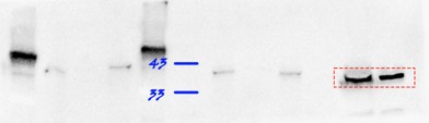
Note: This response was posted by the corresponding author to Review Commons. The content has not been altered except for formatting.
Learn more at Review Commons
Reviewer #1 (Evidence, reproducibility and clarity (Required)):
Summary: This manuscript reports the identification of putative orthologues of mitochondrial contact site and cristae organizing system (MICOS) proteins in Plasmodium falciparum - an organism that unusually shows an acristate mitochondrion during the asexual part of its life cycle and then this develops cristae as it enters the sexual stage of its life cycle and beyond into the mosquito. The authors identify PfMIC60 and PfMIC19 as putative members and study these in detail. The authors at HA tags to both proteins and look for timing of expression during the parasite life cycle and attempt (unsuccessfully) to localise them within the parasite. They also genetically deleted both gene singly and in parallel and phenotyped the effect on parasite development. They show that both proteins are expressed in gametocytes and not asexuals, suggesting they are present at the same time as cristae development. They also show that the proteins are dispensible for the entire parasite life cycle investigated (asexuals through to sporozoites), however there is some reduction in mosquito transmission. Using EM techniques they show that the morphology of gametocyte mitochondria is abnormal in the knock out lines, although there is great variation.
Major comments: The manuscript is interesting and is an intriguing use of a well studied organism of medical importance to answer fundamental biological questions. My main comments are that there should be greater detail in areas around methodology and statistical tests used. Also, the mosquito transmission assays (which are notoriously difficult to perform) show substantial variation between replicates and the statistical tests and data presentation are not clear enough to conclude the reduction in transmission that is claimed. Perhaps this could be improved with clearer text?
We would like to thank the reviewer for taking the time to review our manuscript. We are happy to hear the reviewer thinks the manuscript is interesting and thank the reviewer for their constructive feedback.
To clarify the statistical analyses used, we included a new supplementary dataset with all statistical analyses and p-values indicated per graph. Furthermore, figure legends now include the information on the exact statistical test used in each case.
Regarding mosquito experiments, while we indeed reported a reduction in transmission and oocysts numbers we are aware that this effect might be due to the high variability in mosquito feeding assays. To highlight this point, we deleted the sentence "with the transmission reduction of [numbers]...." and we included the sentence "The high variability encountered in the standard membrane feeding assays, though, partially obstructs a clear conclusion on the biological relevance of the observed reduction in oocyst numbers"
More specific comments to address: Line 101/Fig1E (and figure legend) - What is this heatmap showing. It would be helpful to have a sentence or two linking it to a specific methodology. I could not find details in the M+M section and "specialized, high molecular mass gels" does not adequately explain what experiments were performed. The reference to Supplementary Information 1 also did not provide information.
We added the information "high molecular mass gels with lower acrylamide percentage" to clarify methodology in the text. Furthermore, we extended the figure legend to include all relevant information. Further experimental details can be found in the study cited in this context, where the dataset originates from (Evers et al., 2021).
Line 115 and Supplementary Figure 2C + D - The main text says that the transgenic parasites contained a mitochondrially localized mScarlet for visualization and localization, but in the supplementary figure 2 it shows mitotracker labelling rather than mScarlet. This is very confusing. The figure legend also mentions both mScarlet and MitoTracker. I assume that mScarlet was used to view in regular IFAs (Fig S2C) and the MitoTracker was used for the expansion microscopy (Fig S2D)? Please clarify.
We thank the reviewer for pointing this out - this was indeed incorrectly annotated. We used the endogenous mito-mScarlet signal in IFA and mitoTracker in U-ExM. The figure annotation has now been corrected.
Figure 2C - what is the statistical test being used (the methods say "Mean oocysts per midgut and statistical significance were calculated using a generalized linear mixed effect model with a random experiment effect under a negative binomial distribution." but what test is this?)?
The statistic test is now included in the material and method section with the sentence "The fitted model was used to obtain estimated means and contrasts and were evaluated using Wald Statistics". The test is now also mentioned in the figure legend.
Also the choice of a log10 scale for oocyst intensity is an unusual choice - how are the mosquitoes with 0 oocysts being represented on this graph? It looks like they are being plotted at 10^-1 (which would be 0.1 oocysts in a mosquito which would be impossible).
As the data spans three orders of magnitude with low values being biologically meaningful, we decided that a log scale would best facilitate readability of the graph. As the 0 values are also important to show, we went with a standard approach to handle 0s in log transformed data and substituted the 0s with a small value (0.001). We apologize for not mentioning this transformation in the manuscript. To make this transformation transparent, we added a break at the lower end of the log‑scaled y‑axis and relabelled the lowest tick as '0'. This ensures that mosquitoes with zero oocysts are shown along the x‑axis without being assigned an artificial value on the log scale. We would furthermore like to highlight that for statistics we used the true value 0 and not 0.001.
Figure 2D - it is great that the data from all feeding replicates has been shared, however it is difficult to conclude any meaningful impact in transmission with the knock-out lines when there is so much variation and so few mosquitoes dissected for some datapoints (10 mosquitoes are very small sample sizes). For example, Exp1 shows a clear decrease in mic19- transmission, but then Exp2 does not really show as great effect. Similarly, why does the double knock out have better transmission than the single knockouts? Sure there would be a greater effect?
We agree with the reviewer and with the new sentence added, as per major point, we hope we clarified the concept. Note that original Figure 2D has been moved to the supplementary information, as per minor comment of another reviewer.
Figure 3 legend - Please add which statistical test was used and the number of replicates.
Done
Figure 4 legend - Please add which statistical test was used and the number of replicates.
Done. Regarding replicates, note that while we measured over 100 cristae from over 30 mitochondria, these all stem from the same parasite culture.
Figure 5C - the 3D reconstructions are very nice, but what does the red and yellow coloring show?
Indeed, the information was missing. We added it to the figure legend.
Line 352 - "Still, it is striking that, despite the pronounced morphological phenotype, and the possibly high mitochondrial stress levels, the parasites appeared mostly unaffected in life cycle propagation, raising questions about the functional relevance of mitochondria at these stages." How do the authors reconcile this statement with the proven fact that mitochondria-targeted antimalarials (such as atovaquone) are very potent inhibitors of parasite mosquito transmission?
Our original sentence was reductive. What we wanted to state was related to the functional relevance of crista architecture and overall mitochondrial morphology rather than the general functional relevance of the mitochondria. We changed the sentence accordingly.
Furthermore, even though we do not discuss this in the article, we are aware of mitochondria targeting drugs that are known to block mosquito transmission. We want to point out that it is difficult to discern the disruption of ETC and therefore an impact on energy conversion with the impact on the essential pathway of pyrimidine synthesis, highly relevant in microgamete formation. Still, a recent paper from Sparkes et al. 2024 showed the essentiality of mitochondrial ATP synthesis during gametogenesis so it is very likely that the mitochondrial energy conversion is highly relevant for transmission to the mosquito.
Reviewer #1 (Significance (Required)):
This manuscript is a novel approach to studying mitochondrial biology and does open a lot of unanswered questions for further research directions. Currently there are limitations in the use of statistical tests and detail of methodology, but these could be easily be addressed with a bit more analysis/better explanation in the text. This manuscript could be of interest to readers with a general interest in mitochondrial cell biology and those within the specific field of Plasmodium research. My expertise is in Plasmodium cell biology.
We thank the reviewer for the praise.
Reviewer #2 (Evidence, reproducibility and clarity (Required)):
Major comments: 1) In my opinion, the authors tend to sensationalize or overinterpret their results. The title of the manuscript is very misleading. While MICOS is certainly important for crista formation, it is not the only factor, as ATP synthase dimer rows make a highly significant contribution to crista morphology. Thus, one can argue with equal validity that ATP synthase should be considered the 'architect', as it's the conformation of the dimers and rows modulate positive curvature. Secondly, while cristae are still formed upon mic60/mic19 gene knockout (KO), they are severely deformed, and likely dysfunctional (see below). Thus, I do not agree with the title that MICOS is dispensable for crista formation, because the authors results show that it clearly is essential. So, the title should be changed.
We thank the reviewer for taking the time to review our manuscript.
Based on the reviewers' interpretation we conclude the title does not come across as intended. We have changed the title to: "The role of MICOS in organizing mitochondrial cristae in malaria parasites"
The Discussion section starting from line 373 also suffers from overinterpretation as well as being repetitive and hard to understand. The authors infer that MICOS stability is compromised less in the single KOs (sKO) in compared to the mic60/mic19 double KO (dKO). MICOS stability was never directly addressed here and the composition of the MICOS complex is unaddressed, so it does not make sense to speculate by such tenuous connections. The data suggest to me that mic60 and mic19 are equally important for crista formation and crista junction (CJ) stabilization, and the dKO has a more severe phenotype than either KO, further demonstrating neither is epistatic.
We do agree with the reviewer's notion that we did not address complex stability, and our wording did not make this sufficiently clear. We shortened and rephrased the paragraph in question.
The following paragraphs (line 387 to 422) continues with such unnecessary overinterpretation to the point that it is confusing and contradictory. Line 387 mentions an 'almost complete loss of CJs' and then line 411 mentions an increase in CJ diameter, both upon Mic60 ablation. I do not think this discussion brings any added value to the manuscript and should be shortened. Yes, maybe there are other putative MICOS subunits that may linger in the KOS that are further destabilized in the dKO, or maybe Mic60 remains in the mic19 KO (and vice versa) to somehow salvage more CJs, which is not possible in the dKO. It is impossible to say with confidence how ATP synthase behaves in the KOs with the current data.
We shortened this paragraph.
2) While the authors went through impressive lengths to detect any effect on lifecycle progression, none was found except for a reduction in oocyte count. However, the authors did not address any direct effect on mitochondria, such as OXPHOS complex assembly, respiration, membrane potential. This seems like a missed opportunity, given the team's previous and very nice work mapping these complexes by complexome profiling. However, I think there are some experiments the authors can still do to address any mitochondrial defects using what they have and not resorting to complexome profiling (although this would be definitive if it is feasible):
i) Quantification of MitoTracker Red staining in WT and KOs. The authors used this dye to visualize mitochondria to assay their gross morphology, but unfortunately not to assay membrane potential in the mutants. The authors can compare relative intensities of the different mitochondria types they categorized in Fig. 3A in 20-30 cells to determine if membrane potential is affected when the cristae are deformed in the mutants. One would predict they are affected.
Interesting suggestion. As our staining and imaging conditions are suitable for such analysis (as demonstrated by Sarazin et al., 2025, https://www.biorxiv.org/content/10.1101/2025.11.27.690934v1), we performed the measurements on the same dataset which we collected for Figure 3. We did, however, not detect any difference in mitotracker intensity between the different lines. The result of this analysis is included in the new version of Supplementary figure S6.
ii) Sporozoites are shown in Fig S5. The authors can use the same set up to track their motion, with the hypothesis that they will be slower in the mutants compared to WT due to less ATP. This assumes that sporozoite mitochondria are active as in gametocytes.
While theoretically plausible and informative, we currently do not know the relevance of mitochondrial energy conversion for general sporozoite biology or specifically features of sporozoite movement. Given the required resources and time to set this experiment up and the uncertainty whether it is a relevant proxy for mitochondrial functioning, we argue it is out of scope for this manuscript.
iii) Shotgun proteomics to compare protein levels in mutants compared to WT, with the hypothesis that OXPHOS complex subunits will be destabilized in the mutants with deformed cristae. This could be indirect evidence that OXPHOS assembly is affected, resulting in destabilized subunits that fail to incorporate into their respective complexes.
While this experiment could potentially further our understanding of the interaction between MICOS and levels of OXPHOS complex subunits we argue that the indirect nature of the evidence does not justify the required investments.
To expedite resubmission, the authors can restrict the cell lines to WT and the dKO, as the latter has a stronger phenotype that the individual KOs and conclusions from this cell line are valid for overall conclusions about Plasmodium MICOS.
I will also conclude that complexome/shotgun proteomics may be a useful tool also for identifying other putative MICOS subunits by determining if proteins sharing the same complexome profile as PfMic60 and Mic19 are affected. This would address the overinterpretation problem of point 1.
3) I am aware of the authors previous work in which they were not able to detect cristae in ABS, and thus have concluded that these are truly acristate. This can very well be true, or there can be immature cristae forms that evaded detection at the resolution they used in their volumetric EM acquisitions. The mitochondria and gametocyte cristae are pretty small anyway, so it not unreasonable to assume that putative rudimentary cristae in ABS may be even smaller still. Minute levels of sampled complex III and IV plus complex V dimers in ABS that were detected previously by the authors by complexome profiling would argue for the presence of miniscule and/or very few cristae.
I think that authors should hedge their claim that ABS is acrisate by briefly stating that there still is a possibility that miniscule cristae may have been overlooked previously.
We acknowledge that we cannot demonstrate the absolute absence of any membrane irregularities along the inner mitochondrial membrane. At the same time, if such structures were present, they would be extremely small and unlikely to contain the full set of proteins characteristic of mature cristae. For this reason, we consider it appropriate to classify ABS mitochondria as acristate. To reflect the reviewer's point while maintaining clarity for readers, we have slightly adjusted our wording in the manuscript, changing 'fully acristate' to 'acristate'.
This brings me to the claim that Mic19 and Mic60 proteins are not expressed in ABS. This is based on the lack of signal from the epitope tag; a weak signal is detected in gametocytes. Thus, one can counter that Mic19 and Mic60 are also expressed, but below the expression limits of the assay, as the protein exhibits low expression levels when mitochondrial activity is upregulated.
We agree with the reviewer that the absence of a detectable epitope‑tag signal does not definitively exclude low‑level expression, and we have therefore replaced the term 'absent' with 'undetectable' throughout the manuscript. In context with previous findings of low-level transcripts of the proteins in a study by Lopez-Berragan et al. and Otto et al., we also added the sentence "The apparent absence could indicate that transcripts are not translated in ABS or that the proteins' expression was below detection limits of western blot analysis." to the discussion. _At the same time, we would like to clarify that transcript levels for both genes fall within the
To address this point, the authors should determine of mature mic60 and mic19 mRNAs are detected in ABS in comparison to the dKO, which will lack either transcript. RT-qPCR using polyT primers can be employed to detect these transcripts. If the level of these mRNAs are equivalent to dKO in WT ABS, the authors can make a pretty strong case for the absence of cristae in ABS.
We appreciate the reviewer's suggestion. As noted in the Discussion, existing transcriptomic datasets already show detectable MIC19 and MIC60 mRNAs in ABS. For this reason, we expect RT-qPCR to reveal low (but not absent) levels of both transcripts, unlike the true loss expected to be observed in the dKO. Because such residual signals have been reported previously and their biological relevance remains uncertain, we do not believe transcript levels alone can serve as a definitive indicator of cristae absence in ABS.
They should highlight the twin CX9C motifs that are a hallmark of Mic19 and other proteins that undergo oxidative folding via the MIA pathway. Interestingly, the Mia40 oxidoreductase that is central to MIA in yeast and animals, is absent in apicomplexans (DOI: 10.1080/19420889.2015.1094593).
Searching for the CX9C motifs is a valuable suggestion. In response to the reviewer´s suggestion we analysed the conservation of the motif in PfMIC19 and included this in a new figure panel (Figure 1 F).
Did the authors try to align Plasmodium Mic19 orthologs with conventional Mic19s? This may reveal some conserved residues within and outside of the CHCH domain.
In response to this comment we made Figure 1 F, where we show conserved residues within the CHCH domains of a broad range of MIC19 annotated sequences across the opisthokonts, and show that the Cx9C motifs are conserved also in PfMIC19. Outside the CHCH domain, we did not find any meaningful conservation, as PfMIC19 heavily diverges from opisthokont MIC19.
5) Statistcal significance. Sometimes my eyes see population differences that are considered insignificant by the statistical methods employed by the authors, eg Fig. 4E, mutants compared to WT, especially the dKO. Have the authors considered using other methods such as student t-test for pairwise comparisons?
The graphs in figures 3, 4 and 5 got a makeover, such that they now are in linear scale and violin plots (also following a suggestion from further down in the reviewer's comments). We believe that this improves interpretability. ANOVA was kept as statistical testing to assure the correction for multiple comparisons that cannot be performed with standard t-test. A full overview of statistics and exact p-values can also be found in the newly added supplementary information 2.
Minor comments: Line 33. Anaerobes (eg Giardia) have mitochondria that do produce ATP, unlike aerobic mitochondria
We acknowledge that producing ATP via OXPHOS is not a characteristic of all mitochondria-like organelles (e.g. mitosomes), which is why these are typically classified separately from canonical mitochondria. When not considering mitochondria-like organelles, energy conversion is the function that the mitochondrion is most well-known for and the one associated with cristae.
Line 56: Unclear what authors mean by "canonical model of mitochondria"
To clarify we changed this to "yeast or human" model of mitochondria.
Lines 75-76: This applies to Mic10 only
We removed the "high degree of conservation in other cristate eukaryotes" statement.
Line 80: Cite DOI: 10.1016/j.cub.2020.02.053
Done
Fig 2D: I find this table difficult to read. If authors keep table format, at least get rid of 'mean' column' as this data is better depicted in 2C. I suggest depicted this data either like in 3B depicting portion of infected vs unaffected flies in all experiments, then move modified Table to supplement. Important to point out experiment 5 appears to be an outlier with reduced infectivity across all cell lines, including WT.
To clarify: the mean reported in the table indicates the mean per replicate while the mean reported in figure 2C is the overall mean for a given genotype that corrects for variability within experiments. We agree that moving the table to the supplementary data is a good idea. We decided to not include a graph for infected and non-infected mosquitoes as this information would be partially misleading, highlighting a phenotype we argue to be influenced by the strong variability.
Fig. 3C-G: I feel like these data repeatedly lead to same conclusions. These are all different ways of showing what is depicted in Fig 2B: mitochondria gross morphology is affected upon ablation of MICOS. I suggest that these graphs be moved to supplement and replaced by the beautiful images.
Thank you for the nice comment on our images. We have now moved part of the graphs to supplementary figure 6 and only kept the Relative Frequency, Sphericity and total mitochondria volume per cell in the main figure.
Line 180: Be more specific with which tubulin isoform is used as a male marker and state why this marker was used in supplemental Fig S6.
We have now specified the exact tubulin isoform used as the male gametocyte marker, both in the main text and in Supplementary Fig. S6. This is a commercial antibody previously known to work as an effective male marker, which is why we selected it for this experiment. This is now clearly stated in the manuscript.
Line 196 and Fig 3C: the word 'intensities' in this context is very ambiguous. Please choose a different term (puncta, elements, parts?). This is related to major point 2i above.
To clarify the biological effect that we can conclude form the measurement, we added an explanation about it in the respective section of the results, and we decided to replace the raw results of the plug-in readout with the deduced relative dispersion.
Line 222: Report male/female crista measurements
We added Supplementary information 2, which contains exact statistical test and outcomes on all presented quantifications as well as a per-sex statistical analysis of the data from figure 4. Correspondingly, we extended supplementary information 2 by a per-sex colour code for the thin section TEM data.
Fig. 4B-E: depict data as violin plots or scatter plots like Fig. 2C to get a better grasp of how the crista coverage is distributed. It seems like the data spread is wider in the double KO. This would also solve the problem with the standard deviation extending beyond 0%.
We changed this accordingly.
Lines 331-333: Please clarify that this applies for some, but not all MICOS subunits. Please also see major point 1 above. Also, the authors should point out that despite their structural divergence, trypanosomal cryptic mitofilins Mic34 and Mic40 are essential for parasite growth, in contrast to their findings with PfMic60 (DOI: https://doi.org/10.1101/2025.01.31.635831).
This has been changed accordingly.
Line 320: incorrect citation. Related to point 1above.
Correct citation is now included in the text.
Lines 333-335. This is related to the above. Again, some subunits appear to affect cell growth under lab conditions, and some do not. This and the previous sentence should be rewritten to reflect this.
This has been changed accordingly.
Line 343-345: The sentence and citation 45 are strange. Regarding the former, it is about CHCHD10, whose status as a bona fide MICOS subunit is very tenuous, so I would omit this. About the phenomenon observed, I think it makes more sense to write that Mic60 ablation results in partially fragmented mitochondria in yeast (Rabl et al., 2009 J Cell Biol. 185: 1047-63). A fragmented mitochondria is often a physiological response to stress. I would just rewrite as not to imply that mitochondrial fission (or fusion) is impaired in these KOs, or at least this could be one of several possibilities.
The sentence has been substituted following the indication of the reviewer. Though we still include the data of the human cells as this has also been shown in Stephens et al. 2020.
Line 373: 'This indicates' is too strong. I would say 'may suggest' as you have no proof that any of the KOs disrupts MICOS. This hypothesis can be tested by other means, but not by penetrance of a phenotype.
Done
Line 376-377; 'deplete functionality' does not make sense, especially in the context of talking about MICOS subunit stability. In my opinion, this paragraph overinterprets the KO effects on MICOS stability. None of the experiments address this phenomenon, and thus the authors should not try to interpret their results in this context. See major point 1. Other suggestions for added value
We removed the sentence. Also, the entire paragraph has been shortened, restructured and wording was changed to address major point 1.
1) Does Plasmodium Sam50 co-fractionate with Mic60 and Mic19 in BN PAGE (Fig. 1E)
While we did identify SAMM50 in our BN PAGE, the protein does not co-migrate with the MICOS components but instead comigrates with other components of a putative sorting and assembly machinery (SAM) complex. As SAMM50, the SAM complex and the overarching putative mitochondrial membrane space bridging (MIB) complex are not mentioned in the manuscript, we decided to not include the information in the figure.
Reviewer #2 (Significance (Required)):
The manuscript by Tassan-Lugrezin is predicated on the idea that Plasmodium represents the only system in which de novo crista formation can be studied. They leverage this system to ask the question whether MICOS is essential for this process. They conclude based on their data that the answer is no, which the authors consider unprecedented. But even if their claim is true that ABS is acristate, this supposed advantage does not really bring any meaningful insight into how MICOS works in Plasmodium.
First the positives of this manuscript. As has been the case with this research team, the manuscript is very sophisticated in the experimental approaches that are made. The highlights are the beautiful and often conclusive microscopy performed by the authors. Only the localization of Mic60 and Mic19 was inconclusive due to their very low expression unfortunately.
The examination of the MICOS mutants during in vitro life cycle of Plasmodium falciparum is extremely impressive and yields convincing results. Mitochondrial deformation is tolerated by life cycle stage differentiation, with a modest but significant reduction of oocyte production, being observed.
However, despite the herculean efforts of the authors, the manuscript as it currently stands represents only a minor advance in our understanding of the evolution of MICOS, which from the title and focus of the manuscript, is the main goal of the authors. In its current form, the manuscript reports some potentially important findings:
1) Mic60 is verified to play a role in crista formation, as is predicted by its orthology to other characterized Mic60 orthologs.
2) The discovery of a novel Mic19 analog (since the authors maintain there is no significant sequence homology), which exhibits a similar (or the same?) complexome profile with Mic60. This protein was upregulated in gametocytes like Mic60 and phenocopies Mic60 KO.
3) Both of these MICOS subunits are essential (not dispensable) for proper crista formation
4) Surprisingly, neither MICOS subunit is essential for in vitro growth or differentiation from ABS to sexual stages, and from the latter to sporozoites. This says more about the biology of plasmodium itself than anything about the essentiality of Mic60, ie plasmodium life cycle progression tolerates defects to mitochondrial morphology. But yes, I agree with the authors that Mic60's apparent insignificance for cell growth in examined conditions does differ with its essentiality in other eukaryotes. But fitness costs were not assayed (eg by competition between mutants and WT in infection of mosquitoes)
5) Decreased fitness of the mutants is implied by a reduction of oocyte formation.
While interesting in their own way, collectively they do not represent a major advance in our understanding of MICOS evolution. Furthermore, the findings bifurcate into categories informing MICOS or Plasmodium biology. Both aspects are somewhat underdeveloped in their current form.
This is unfortunate because there seem to be many missed opportunities in the manuscript that could, with additional experiments, lead to a manuscript with much wider impact. For me, what is remarkable about Plasmodium MICOS that sets it apart from other iterations is the apparent absence of the Mic10 subunit. Purification of plasmodium MICOS via the epitope tagged Mic60 and Mic19 could have verified that MICOS is assembled without this core subunit. Perhaps Mic60 and Mic19 are the vestiges of the complex, and thus operate alone in shaping cristae. Such a reduction may also suggest the declining importance of mitochondria in plasmodium.
Another missed opportunity was to assay the impact of MICOS-depletion of OXPHOS in plasmodium. This is a salient issue as maybe crista morphology is decoupled from OXPHOS capacity in Plasmodium, which links to the apparent tolerance of mitochondrial morphology in cell growth and differentiation. I suggested in section A experiments to address this deficit.
Finally, the authors could assay fitness costs of MICOS-ablation and associated phenotypes by assaying whether mosquito infectivity is reduced in the mutants when they are directly competing with WT plasmodium. Like the authors, I am also surprised that MICOS mutants can pass population bottlenecks represented by differentiation events. Perhaps the apparent robustness of differentiation may contribute plasmodium's remarkable ability to adapt.
I realize that the authors put a lot of efforts into their study and again, I am very impressed by the sophistication of the methods employed. Nevertheless, I think there is still better ways to increase the impact of the study aside from overinterpreting the conclusions from the data. But this would require more experiments along the lines I suggest in Section A and here.
We thank the reviewer for their extensive analysis of the significance of our findings, including the compliments on our microscopy images and the sophisticated experimental approaches. We hope we have convincingly argued why we could or could not include some of the additional analyses suggested by the reviewer in section 1 above.
With regard to the significance statement, we want to point out that our finding that PfMICOS is not needed for initial formation of cristae (as opposed to organization thereof), is a confirmation of something that has been assumed by the field, without being the actual focus of studies. We argue that the distinction between formation and organization of cristae is important and deserves some attention within the manuscript. The result of MICOS not being involved in the initial formation of cristae, we argue to be relevant in Plasmodium biology and beyond. As for the insights into how MICOS works in Plasmodium we have confirmed that the previously annotated PfMIC60 is indeed involved in the organization of cristae. Furthermore, we have identified and characterized PfMIC19. These findings, we argue, are indeed meaningful insights into PfMICOS.
Reviewer #3 (Evidence, reproducibility and clarity (Required)):
Summary:
MICOS is a conserved mitochondrial protein complex responsible for organising the mitochondrial inner membrane and the maintenance of cristae junctions. This study sheds first light on the role of two MICOS subunits (Mic60 and the newly annotated Mic19) in the malaria parasite Plasmodium falciparum, which forms cristae de novo during sexual development, as demonstrated by EM of thin section and electron tomography. By generating knockout lines (including a double knockout), the authors demonstrate that knockout of both MICOS subunits leads to defects in cristae morphology and a partial loss of cristae junctions. With a formidable set of parasitological assays, the authors show that despite the metabolically important role of mitochondria for gametocytes, the knockout lines can progress through the life stages and form sporozoites, albeit with diminished infection efficiency.
We thank the reviewer for their time and compliment.
Major comments:
1) The authors should improve to present their findings in the right context, in particular by:
(i) giving a clearer description in the introduction of what is already known about the role of MICOS. This starts in the introduction, where one main finding is missing: loss of MICOS leads to loss of cristae junctions and the detachment of cristae membranes, which are nevertheless formed, but become membrane vesicles. This needs to be clearly stated in the introduction to allow the reader to understand the consistency of the authors' findings in P. falciparum with previous reports in the literature.
We extended the introduction to include this information.
(ii) at the end to the introduction, the motivating hypothesis is formulated ad hoc "conclusive evidence about its involvement in the initial formation of cristae is still lacking" (line 83). If there is evidence in the literature that MICOS is strictly required for cristae formation in any organism, then this should be explained, because the bona fide role of MICOS is maintenance of cristae junctions (the hypothesis is still plausible and its testing important).
To clarify we rephrased the sentence to: "Although MICOS has been described as an organizer of crista junctions, its role during the initial formation of nascent cristae has not been investigated."
2) Line 96-97: "Interestingly, PfMIC60 is much larger than the human MICOS counterpart, with a large, poorly predicted N-terminal extension." This statement is lacking a reference and presumably refers to annotated ORFs. The authors should clarify if the true N-terminus is definitely known - a 120kDa size is shown for the P. falciparum but this is not compared to the expected length or the size in S. cerevisiae.
To solve the reference issue, we added the uniprot IDs we compared to see that the annotated ORF is bigger in Plasmodium. We also changed the comparison to yeast instead of human, because we realized it is confusing to compare to yeast all throughout the figure, but then talk about human in this specific sentence.
Regarding whether the true N-terminus is known. Short answer: No, not exactly.
However, we do know that the Pf version is about double the size of the yeast protein.
As the reviewer correctly states, we show the size of 120kDa for the tagged protein in Figure 1G. Considering that we tagged the protein C-terminally, and observed a 120kDa product on western blot, it is safe to conclude that the true N-terminus does not deviate massively from the annotated ORF, and hence, that there is a considerable extension of the protein beyond a 60kDa protein. We do not directly compare to yeast MIC60 on our western blots, however, that comparison can be drawn from literature: Tarasenko et al., 2017 showed that purified MIC60 running at ~60kDa on SDS-PAGE actively bends membranes, suggesting that in its active form, the monomer of yeast MIC60 is indeed 60kDa in size.
To clarify, we now emphasize that we ran the Alphafold prediction on the annotated open reading frame (annotated and sequenced by Bohme et al. and Chapell et al. now cited in the manuscript), and revised the wording to make clear what we are comparing in which sentence.
3) lines 244-245: "Furthermore, our data indicates the effect size increases with simultaneous ablation of both proteins?". The authors should explain which data they are referring to, as some of the data in Fig 3 and 4 look similar and all significance tests relate to the wild type, not between the different mutants, so it is not clear if any overserved differences are significant. The authors repeat this claim in the discussion in lines 368-369 without referring to a specific significance test. This needs to be clarified.
As a reply to this and other comments from the reviewers we added the multiple testing within all samples. In addition, to clarify statistics used we included a supplementary dataset with all p-values and statistical tests used.
4) lines 304-306: "Though well established as the cristae organizing system, the role of MICOS in initial formation of cristae remains hidden in model organisms that constitutively display cristae.". This sentence is misleading since even in organisms that display numerous cristae throughout their life cycle, new cristae are being formed as the cells proliferate. Thus, failure to produce cristae in MICOS knockout lines would have been observable but has apparently not been reported in the literature. Thus, the concerted process in P. falciparum makes it a great model organism, but not fundamentally different to what has been studied before in other organisms.
We deleted this statement.
5) lines 373-378. "where ablation of just MIC60 is sufficient to deplete functionality of the entire MICOS (11, 15),". The authors' claim appears to be contrary to what is actually stated in ref 15, which they cite:
"MICOS subunits have non-redundant functions as the absence of both MICOS subcomplexes results in more severe morphological and respiratory growth defects than deletion of single MICOS subunits or subcomplexes."
This seems in line with what the authors show, rather than "different".
This sentence has been removed.
6) lines 380-385: "... thus suggesting that membrane invaginations still arise, but are not properly arranged in these knockout lines. This suggests that MICOS either isn't fully depleted,...". These conclusions are incompatible with findings from ref. 15, which the authors cite. In that study, the authors generated a ∆MICOS line which still forms membrane invaginations, showing that MICOS is not required at all for this process in yeast. Hence the authors' implication that MICOS needs to be fully depleted before membrane invaginations cease to occur is not supported by the literature.
This sentence has been deleted in the revised version of the manuscript.
Minor comments:
7) The authors should consider if the first part of their title could be seen as misleading: It suggests that MICOS is "the architect" in cristae formation, but this is not consistent with the literature nor their own findings.
Title is changed accordingly
Minor comments:
- Line 43, of the three seminal papers describing the discovery of MICOS in 2011, the authors only cite two (refs 6 and 7), but miss the third paper, Hoppins et al, PMID: 21987634, which should probably be corrected.
Done, the paper is now cited
- Page 2, line 58: for a more complete picture the authors should also cite the work of others here which shows that although at very low levels, e.g. complex III (a drug target) and ATP synthase do assemble (Nina et al, 2011, JBC).
Done
- Page 3, line 80: "Irrespective of the shape of an organism's cristae, the crista junctions have been described as tubular channels that connect the cristae membrane to the inner boundary membrane (22, 24)." This omits the slit-shaped cristae junctions found in yeast (Davies et al, 2011, PNAS), which the authors should include.
The paper and concept have been added to the manuscript, though the sentence has been moved up in the introduction, when crista junctions are first introduced.
- Line 97: "poorly predicted N-terminal extension", as there is no experimental structure, we don't know if the prediction is poor. Presumably the authors mean either poorly ordered or the absence of secondary structure elements, or the poor confidence score for that region in the prediction? This should be clarified or corrected.
We were referring to the poor confidence score. To address this comment as well as major point 2, we rewrote the respective paragraph. It now clearly states that confidence of the prediction is low, and we mention the tool that was used to identify conserved domains (Topology-based Evolutionary Domains).
- Line 98: "an antiparallel array of ten β-sheets". They are actually two parallel beta-sheets stacked together. The authors could find out the name of this fold, but the confidence of the prediction is marked a low/very low. So, its existence is unknown, not just its "function".
We adapted the domain description to "a stack of two parallel beta-sheets" and replaced the statement on unknown function by the statement "Because this domain is predicted solely from computational analysis, both its actual existence in the native protein and its biological function remain unknown."
Fig 1B: The authors show two alphafold predictions of S. cerevisiae and P. falciparum Mic60 structures. There is however an experimental Mic60/19 (fragment) structure from the former organism (PMID: 36044574), which should be included if possible
We appreciate the reviewer's suggestion and note that the available structural data indeed provides valuable insight into how MIC60 and MIC19 interact. However, these structures represent fusion constructs of limited protein fragments and therefore capture only a small portion of each protein, specifically the interaction interface. Because our aim in Fig. 1B is to compare the overall domain architecture of the full‑length proteins, we believe that including fragment‑based structures would be less informative in this context.
Line: 318-321: "The same trend was observed for PfMIC19 and PfMIC60. Although transcriptomic data suggested that low-level transcripts of PfMIC19 and PfMIC60 are present in ABS (38), we did not detect either of the proteins in ABS by western blot analysis. While this statement is true, the authors should comment on the sensitivity of the respective methods - how well was the antibody working in their hands and how do they interpret the absence of a WB band compared to transcriptomics data?
The HA antibody used in our experiments is a standard commercial reagent that performs reliably in both WB and IFA, although it shows a low background signal in gametocytes. We agree that the sensitivity of the method and the interpretation of weak or absent bands should be addressed explicitly. Transcript levels for both PfMIC19 and PfMIC60 in asexual blood stages fall within the
- Lines 322-323: would the authors not typically have expected an IFA signal given the strength of the band in Western blot? If possible, the authors should comment if the negative fluorescence outcome can indeed be explained with the low abundance or if technical challenges are an equally good explanation.
Considering the nature of the investigated proteins (embedded in the IMM and spread throughout the mitochondria) difficulties in achieving a clear signal in IFA or U-ExM are not very surprizing. While epitopes may remain buried in IFA, U-ExM usually increases accessibility for the antibodies. However, U-ExM comes at the cost of being prone to dotty background signals, therefore potentially hiding low abundance, naturally dotty signals such as the signal of MICOS proteins that localize to distinct foci (at the CJ) along the mitochondrion. Current literature suggests that, in both human and yeast, STED is the preferred method for accurate spatial resolution of MICOS proteins (https://www.ncbi.nlm.nih.gov/pubmed/32567732,https://www.ncbi.nlm.nih.gov/pubmed/32067344). Unfortunately, we do not have experience with, nor access to, this particular technique/method.
Lines 357-365: the authors describe limitations of the applied methods adequately. Perhaps it would be helpful to make a similar statement about the analysis of 3D objects like mitochondria and cristae from 2D sections. E.g. the apparent cristae length depends on whether cristae are straight (e.g. coiled structures do not display long cross sections despite their true length in 3D).
The limitations of other methods are described in the respective results section.
We added a clarifying sentence in the results section of Figure 4:
"Note that such measurements do not indicate the true total length or width of cristae, as the data is two-dimensional. The recorded values are to be considered indicative of possible trends, rather than absolute dimensions of cristae."
This statement refers to the length/width measurements of cristae.
In the context of Figure 4 D we mention the following (see preprint lines 229 - 230): "We expect this effect to translate into the third dimension and thus conclude that the mean crista volume increases with the loss of either PfMIC19,PfMIC60, or both."
For Figure 5, we included a clarifying statement in the results section of the preprint (lines 269 - 273): "Note that these mitochondrial volumes are not full mitochondria, but large segments thereof. As a result of the incompleteness of the mitochondria within the section, and the tomography specific artefact of the missing wedge, we were unable to confirm whether cristae were in fact fully detached from the boundary membrane, or just too long to fit within the observable z-range. "
Line 404: perhaps undetected or similar would be a better description than "hidden"?
The sentence does not exist in the revised manuscript
Reviewer #3 (Significance (Required)):
The main strength of the study is that it provides the first characterisation of the MICOS complex in P. falciparum, a human parasite in which the mitochondrion has been shown to be a drug target. Mic60 and the newly annotated Mic19 are confirmed to be essential for proper cristae formation and morphology, as well as overall mitochondrial morphology. Furthermore, the mutant lines are characterised for their ability to complete the parasite life cycle and defects in infection effectivity are observed. This work is an important first step for deciphering the role of MICOS in the malaria parasite and the composition and function of this complex in this organism. The limitation of the study stems from what is already known about MICOS and its subunits in
great detail in yeast and humans with similar findings regarding loss of cristae and cristae defects. The findings of this study do not provide dramatic new insight on MICOS function or go substantially beyond the vast existing literature in terms of the extent of the study, which focuses on parasitological assays and morphological analysis. Exploring the role of MICOS in an early-divergent organism and human parasite is however important given the divergence found in mitochondrial biology and P. falciparum is a uniquely suited model system. One aspect that would increase the impact of the paper would be if the authors could mechanistically link the observed morphological defects to the decreased infection efficiency, e.g. by probing effects on mitochondrial function. This will likely be challenging as the morphological defects are diverse and the fitness defects appear moderate/mild.
As suggested by Reviewer 2, we examined mitochondrial membrane potential in gametocytes using MitoTracker staining and did not observe any obvious differences associated with the morphological defects. At present, additional assays to probe mitochondrial function in P. falciparum gametocytes are not sufficiently established, and developing and validating such methods would require substantial work before they could be applied to our mutant lines. For these reasons, a more detailed mechanistic link between the observed morphological changes and the reduced infection efficiency is currently beyond reach.
The advance presented in this study is to pioneer the study of MICOS in P. falciparum, thus widening our understanding of the role of this complex to different model organism. This study will likely be mainly of interest for specialised audiences such as basic research parasitologists and mitochondrial biologists. My own field of expertise is mitochondrial biology and structural biology.
Author response:
The following is the authors’ response to the original reviews.
Reviewer #1 (Public review):
(1) I have to admit that it took a few hours of intense work to understand this paper and to even figure out where the authors were coming from. The problem setting, nomenclature, and simulation methods presented in this paper do not conform to the notation common in the field, are often contradictory, and are usually hard to understand. Most importantly, the problem that the paper is trying to solve seems to me to be quite specific to the particular memory study in question, and is very different from the normal setting of model-comparative RSA that I (and I think other readers) may be more familiar with.
We have revised the paper for clarity at all levels: motivation, application, and parameterization. We clarify that there is a large unmet need for using RSA in a trial-wise manner, and that this approach indeed offers benefits to any team interested in decoding trial-wise representational information linked to a behavioral responses, and as such is not a problem specific to a single memory study.
(2) The definition of "classical RSA" that the authors are using is very narrow. The group around Niko Kriegeskorte has developed RSA over the last 10 years, addressing many of the perceived limitations of the technique. For example, cross-validated distance measures (Walther et al. 2016; Nili et al. 2014; Diedrichsen et al. 2021) effectively deal with an uneven number of trials per condition and unequal amounts of measurement noise across trials. Different RDM comparators (Diedrichsen et al. 2021) and statistical methods for generalization across stimuli (Schütt et al. 2023) have been developed, addressing shortcomings in sensitivity. Finally, both a Bayesian variant of RSA (Pattern component modelling, (Diedrichsen, Yokoi, and Arbuckle 2018) and an encoding model (Naselaris et al. 2011) can effectively deal with continuous variables or features across time points or trials in a framework that is very related to RSA (Diedrichsen and Kriegeskorte 2017). The author may not consider these newer developments to be classical, but they are in common use and certainly provide the solution to the problems raised in this paper in the setting of model-comparative RSA in which there is more than one repetition per stimulus.
We appreciate the summary of relevant literature and have included a revised Introduction to address this bounty of relevant work. While much is owed to these authors, new developments from a diverse array of researchers outside of a single group can aid in new research questions, and should always have a place in our research landscape. We owe much to the work of Kriegeskorte’s group, and in fact, Schutt et al., 2023 served as a very relevant touchpoint in the Discussion and helped to highlight specific needs not addressed by the assessment of the “representational geometry” of an entire presented stimulus set. Principal amongst these needs is the application of trial-wise representational information that can be related to trial-wise behavioral responses and thus used to address specific questions on brain-behavior relationships. We invite the Reviewer to consider the utility of this shift with the following revisions to the Introduction.
Page 3. “Recently, methodological advancements have addressed many known limitations in cRSA. For example, cross-validated distance measures (e.g., Euclidean distance) have improved the reliability of representational dissimilarities in the presence of noise and trial imbalance (Walther et al., 2016; Nili et al., 2014; Diedrichsen et al., 2021). Bayesian approaches such as pattern component modeling (Diedrichsen, Yokoi, & Arbuckle, 2018) have extended representational approaches to accommodate continuous stimulus features or temporal variation. Further, model comparison RSA strategies (Diedrichsen et al., 2021) and generalization techniques across stimuli (Schütt et al., 2023) have improved sensitivity and inference. Nevertheless, a common feature shared across most of improvements is that they require stimuli repetition to examine the representational structure. This requirement limits their ability to probe brain-behavior questions at the level of individual events”.
Page 8. “While several extensions of RSA have addressed key limitations in noise sensitivity, stimulus variance, and modeling (e.g., Diedrichsen et al., 2021; Schütt et al., 2023), our tRSA approach introduces a new methodological step by estimating representational strength at the trial level. This accounts for the multi-level variance structure in the data, affords generalizability beyond the fixed stimulus set, and allows one to test stimulus- or trial-level modulations of neural representations in a straightforward way”.
Page 44. “Despite such prevalent appreciation for the neurocognitive relevance of stimulus properties, cRSA often does not account for the fact that the same stimulus (e.g., “basketball”) is seen by multiple subjects and produces statistically dependent data, an issue addressed by Schütt et al., 2023, who developed cross validation and bootstrap methods that explicitly model dependence across both subjects and stimulus conditions”.
(3) The stated problem of the paper is to estimate "representational strength" in different regions or conditions. With this, the authors define the correlation of the brain RDM with a model RDM. This metric conflates a number of factors, namely the variances of the stimulus-specific patterns, the variance of the noise, the true differences between different dissimilarities, and the match between the assumed model and the data-generating model. It took me a long time to figure out that the authors are trying to solve a quite different problem in a quite different setting from the model-comparative approach to RSA that I would consider "classical" (Diedrichsen et al. 2021; Diedrichsen and Kriegeskorte 2017). In this approach, one is trying to test whether local activity patterns are better explained by representation model A or model B, and to estimate the degree to which the representation can be fully explained. In this framework, it is common practice to measure each stimulus at least 2 times, to be able to estimate the variance of noise patterns and the variance of signal patterns directly. Using this setting, I would define 'representational strength" very differently from the authors. Assume (using LaTeX notation) that the activity patterns $y_j,n$ for stimulus j, measurement n, are composed of a true stimulus-related pattern ($u_j$) and a trial-specific noise pattern ($e_j,n$). As a measure of the strength of representation (or pattern), I would use an unbiased estimate of the variance of the true stimulus-specific patterns across voxels and stimuli ($\sigma^2_{u}$). This estimator can be obtained by correlating patterns of the same stimuli across repeated measures, or equivalently, by averaging the cross-validated Euclidean distances (or with spatial prewhitening, Mahalanobis distances) across all stimulus pairs. In contrast, the current paper addresses a specific problem in a quite specific experimental design in which there is only one repetition per stimulus. This means that the authors have no direct way of distinguishing true stimulus patterns from noise processes. The trick that the authors apply here is to assume that the brain data comes from the assumed model RDM (a somewhat sketchy assumption IMO) and that everything that reduces this correlation must be measurement noise. I can now see why tRSA does make some sense for this particular question in this memory study. However, in the more common model-comparative RSA setting, having only one repetition per stimulus in the experiment would be quite a fatal design flaw. Thus, the paper would do better if the authors could spell the specific problem addressed by their method right in the beginning, rather than trying to set up tRSA as a general alternative to "classical RSA".
At a general level, our approach rests on the premise that there is meaningful information present in a single presentation of a given stimulus. This assumption may have less utility when the research goals are more focused on estimating the fidelity of signal patterns for RSA, as in designs with multiple repetitions. But it is an exaggeration to state that such a trial-wise approach cannot address the difference between “true” stimulus patterns and noise. This trial-wise approach has explicit utility in relating trial-wise brain information to trial-wise behavior, across multiple cognitions (not only memory studies, as applied here). We have added substantial text to the Introduction distinguishing cRSA, which is widely employed, often in cases with a single repetition per stimulus, and model comparative methods that employ multiple repetitions. We clarify that we do not consider tRSA an alternative to the model comparative approach, and discuss that operational definitions of representational strength are constrained by the study design.
Page 3. “In this paper, we present an advancement termed trial-level RSA, or tRSA, which addresses these limitations in cRSA (not model comparison approaches) and may be utilized in paradigms with or without repeated stimuli”.
Page 4. “Representational geometry usually refers to the structure of similarities among repeated presentations of the same stimulus in the neural data (as captured in the brain RSM) and is often estimated utilizing a model comparison approach, whereas representational strength is a derived measure that quantifies how strongly this geometry aligns with a hypothesized model RSM. In other words, geometry characterizes the pattern space itself, while representational strength reflects the degree of correspondence between that space and the theoretical model under test”.
Finally, we clarified that in our simulation methods we assume a true underlying activity pattern and a random error pattern. The model RSM is computed based on the true pattern, whereas the brain RSM comes from the noisy pattern, not the model RSM itself.
Page 9. “Then, we generated two sets of noise patterns, which were controlled by parameters σ<sub>A</sub> and σ<sub>B</sub> , respectively, one for each condition”.
(4) The notation in the paper is often conflicting and should be clarified. The actual true and measured activity patterns should receive a unique notation that is distinct from the variances of these patterns across voxels. I assume that $\sigma_ijk$ is the noise variances (not standard deviation)? Normally, variances are denoted with $\sigma^2$. Also, if these are variances, they cannot come from a normal distribution as indicated on page 10. Finally, multi-level models are usually defined at the level of means (i.e., patterns) rather than at the level of variances (as they seem to be done here).
We have added notations for true and measured activity patterns to differentiate it from our notation for variance. We agree that multilevel models are usually defined at the level of means rather than at the level of variances and we include a Figure (Fig 1D) that describes the model in terms of the means. We clarify that the σ ($\sigma$) used in the manuscript were not variances/standard deviations themselves; rather, they were meant to denote components of the actual (multilevel) variance parameter. Each component was sampled from normal distributions, and they collectively summed up to comprise the final variance parameter for each trial. We have modified our notation for each component to the lowercase letter s to minimize confusion. We have also made our R code publicly available on our lab github, which should provide more clarity on the exact simulation process.
(5) In the first set of simulations, the authors sampled both model and brain RSM by drawing each cell (similarity) of the matrix from an independent bivariate normal distribution. As the authors note themselves, this way of producing RSMs violates the constraint that correlation matrices need to be positive semi-definite. Likely more seriously, it also ignores the fact that the different elements of the upper triangular part of a correlation matrix are not independent from each other (Diedrichsen et al. 2021). Therefore, it is not clear that this simulation is close enough to reality to provide any valuable insight and should be removed from the paper, along with the extensive discussion about why this simulation setting is plainly wrong (page 21). This would shorten and clarify the paper.
We have added justification of the mixed-effects model given the potential assumption violations. We caution readers to investigate the robustness of their models, and to employ permutation testing that does not make independence assumptions. We have also added checks of the model residuals and an example of permutation testing in the Appendix. Finally, we agree that the first simulation setting does not possess several properties of realistic RDMs/RSMs; however, we believe that there is utility in understanding the mathematical properties of correlations – an essential component of RSA – in a straightforward simulation where the ground truth is known, thus moving the simulation to Appendix 1.
(6) If I understand the second simulation setting correctly, the true pattern for each stimulus was generated as an NxP matrix of i.i.d. standard normal variables. Thus, there is no condition-specific pattern at all, only condition-specific noise/signal variances. It is not clear how the tRSA would be biased if there were a condition-specific pattern (which, in reality, there usually is). Because of the i.i.d. assumption of the true signal, the correlations between all stimulus pairs within conditions are close to zero (and only differ from it by the fact that you are using a finite number of voxels). If you added a condition-specific pattern, the across-condition RSA would lead to much higher "representational strength" estimates than a within-condition RSA, with obvious problems and biases.
The Reviewer is correct that the voxel values in the true pattern are drawn from i.i.d. standard normal distributions. We take the Reviewer’s suggestion of “condition-specific pattern” to mean that there could be a condition-voxel interaction in two non-mutually exclusive ways. The first is additive, essentially some common underlying multi-voxel pattern like [6, 34, -52, …, 8] for all condition A trials, and different one such pattern for condition B trials, etc. The second is multiplicative, essentially a vector of scaling factors [x1.5, x0.5, x0.8, …, x2.7] for all condition A trials, and a different one such vector for condition B trials, etc. Both possibilities could indeed affect tRSA as much as it would cRSA.
Importantly, If such a strong condition-specific pattern is expected, one can build a condition-specific model RDM using one-shot coding of conditions (see example figure; src: https://www.newbi4fmri.com/tutorial-9-mvpa-rsa), to either capture this interesting phenomenon or to remove this out as a confounding factor. This practice has been applied in multiple regression cRSA approaches (e.g., Cichy et al., 2013) and can also be applied to tRSA.
(7) The trial-level brain RDM to model Spearman correlations was analyzed using a mixed effects model. However, given the symmetry of the RDM, the correlations coming from different rows of the matrix are not independent, which is an assumption of the mixed effect model. This does not seem to induce an increase in Type I errors in the conditions studied, but there is no clear justification for this procedure, which needs to be justified.
We appreciate this important warning, and now caution readers to investigate the robustness of their models, and consider employing permutation testing that does not make independence assumptions. We have also added checks of the model residuals and an example of permutation testing in the supplement.
Page 46. “While linear mixed-effects modeling offers a powerful framework for analyzing representational similarity data, it is critical that researchers carefully construct and validate their models. The multilevel structure of RSA data introduces potential dependencies across subjects, stimuli, and trials, which can violate assumptions of independence if not properly modeled. In the present study, we used a model that included random intercepts for both subjects and stimuli, which accounts for variance at these levels and improves the generalizability of fixed-effect estimates. Still, there is a potential for systematic dependence across trials within a subject. To ensure that the model assumptions were satisfied, we conducted a series of diagnostic checks on an exemplar ROI (right LOC; middle occipital gyrus) in the Object Perception dataset, including visual inspection of residual distributions and autocorrelation (Appendix 3, Figure 13). These diagnostics supported the assumptions of normality, homoscedasticity, and conditional independence of residuals. In addition, we conducted permutation-based inference, similar to prior improvements to cRSA (Niliet al. 2014), using a nested model comparison to test whether the mean similarity in this ROI was significantly greater than zero. The observed likelihood ratio test statistic fell in the extreme tail of the null distribution (Appendix 3, Figure 14), providing strong nonparametric evidence for the reliability of the observed effect. We emphasize that this type of model checking and permutation testing is not merely confirmatory but can help validate key assumptions in RSA modeling, especially when applying mixed-effects models to neural similarity data. Researchers are encouraged to adopt similar procedures to ensure the robustness and interpretability of their findings”.
Exemplar Permutation Testing
To test whether the mean representational strength in the ROI right LOC (middle occipital gyrus) was significantly greater than zero, we used a permutation-based likelihood ratio test implemented via the permlmer function. This test compares two nested linear mixed-effects models fit using the lmer function from the lme4 package, both including random intercepts for Participant and Stimulus ID to account for between-subject and between-item variability.
The null model excluded a fixed intercept term, effectively constraining the mean similarity to zero after accounting for random effects:
ROI ~ 0 + (1 | Participant) + (1 | Stimulus)
The full model included the same random effects structure but allowed the intercept to be freely estimated:
ROI ~ 1 + (1 | Participant) + (1 | Stimulus)
By comparing the fit of these two models, we directly tested whether the average similarity in this ROI was significantly different from zero. Permutation testing (1,000 permutations) was used to generate a nonparametric p-value, providing inference without relying on normality assumptions. The full model, which estimated a nonzero mean similarity in the right LOC (middle occipital gyrus), showed a significantly better fit to the data than the null model that fixed the mean at zero (χ²(1) = 17.60, p = 2.72 × 10⁻⁵). The permutation-based p-value obtained from permlmer confirmed this effect as statistically significant (p = 0.0099), indicating that the mean similarity in this ROI was reliably greater than zero. These results support the conclusion that the right LOC contains representational structure consistent with the HMAXc2 RSM. A density plot of the permuted likelihood ratio tests is plotted along with the observed likelihood ratio test in Appendix 3 Figure 14.
(8) For the empirical data, it is not clear to me to what degree the "representational strength" of cRSA and tRSA is actually comparable. In cRSA, the Spearman correlation assesses whether the distances in the data RSM are ranked in the same order as in the model. For tRSA, the comparison is made for every row of the RSM, which introduces a larger degree of flexibility (possibly explaining the higher correlations in the first simulation). Thus, could the gains presented in Figure 7D not simply arise from the fact that you are testing different questions? A clearer theoretical analysis of the difference between the average row-wise Spearman correlation and the matrix-wise Spearman correlation is urgently needed. The behavior will likely vary with the structure of the true model RDM/RSM.
We agree that the comparability between mean row-wise Spearman correlations and the matrix-wise Spearman correlation is needed. We believe that the simulations are the best approach for this comparison, since they are much more robust than the empirical dataset and have the advantage of knowing the true pattern/noise levels. We expand on our comparison of mean tRSA values and matrix-wise Spearman correlations on page 42.
Page 42. “Although tRSA and cRSA both aim to quantify representational strength, they differ in how they operationalize this concept. cRSA summarizes the correspondence between RSMs as a single measure, such as the matrix-wise Spearman correlation. In contrast, tRSA computes such correspondence for each trial, enabling estimates at the level of individual observations. This flexibility allows trial-level variability to be modeled directly, but also introduces subtle differences in what is being measured. Nonetheless, our simulations showed that, although numerical differences occasionally emerged—particularly when comparing between-condition tRSA estimates to within-condition cRSA estimates—the magnitude of divergence was small and did not affect the outcome of downstream statistical tests”.
(9) For the real data, there are a number of additional sources of bias that need to be considered for the analysis. What if there are not only condition-specific differences in noise variance, but also a condition-specific pattern? Given that the stimuli were measured in 3 different imaging runs, you cannot assume that all measurement noise is i.i.d. - stimuli from the same run will likely have a higher correlation with each other.
We recognize the potential of condition-specific patterns and chose to constrain the analyses to those most comparable with cRSA. However, depending on their hypotheses, researchers may consider testing condition RSMs and utilizing a model comparison approach or employ the z-scored approach, as employed in the simulations above. Regarding the potential run confounds, this is always the case in RSA and why we exclude within-run comparisons. We have also added to the Discussion the suggestion to include run as a covariate in their mixed-effects models. However, we do not employ this covariate here as we preferred the most parsimonious model to compare with cRSA.
Page 46 - 47. “Further, while analyses here were largely employed to be comparable with cRSA, researchers should consider taking advantage of the flexibility of the mixed-effects models and include co variates of non-interest (run, trial order etc.)”.
(10) The discussion should be rewritten in light of the fact that the setting considered here is very different from the model-comparative RSA in which one usually has multiple measurements per stimulus per subject. In this setting, existing approaches such as RSA or PCM do indeed allow for the full modelling of differences in the "representational strength" - i.e., pattern variance across subjects, conditions, and stimuli.
We agree that studies advancing designs with multiple repetitions of a given stimulus image are useful in estimating the reliability of concept representations. We would argue however that model comparison in RSA is not restricted to such data. Many extant studies do not in fact have multiple repetitions per stimulus per subject (Wang et al., 2018 https://doi.org/10.1088/1741-2552/abecc3, Gao et al, 2022 https://doi.org/10.1093/cercor/bhac058, Li et al, 2022 https://doi.org/10.1002/hbm.26195, Staples & Graves, 2020 https://doi.org/10.1162/nol_a_00018) that allow for that type of model-comparative approach. While beneficial in terms of noise estimation, having multiple presentations was not a requirement for implementing cRSA (Kriegeskorte, 2008 https://doi.org/10.3389/neuro.06.004.2008). The aim of this manuscript is to introduce the tRSA approach to the broad community of researchers whose research questions and datasets could vary vastly, including but not limited to the number of repeated presentations and the balance of trial counts across conditions.
(11) Cross-validated distances provide a powerful tool to control for differences in measurement noise variances and possible covariances in measurement noise across trials, which has many distinct advantages and is conceptually very different from the approach taken here.
We have added language on the value of cross-validation approaches to RSA in the Discussion:
Page 47. “Additionally, we note that while our proposed tRSA framework provides a flexible and statistically principled approach for modeling trial-level representational strength, we acknowledge that there are alternative methods for addressing trial-level variability in RSA. In particular, the use of cross-validated distance metrics (e.g., crossnobis distance) has become increasingly popular for controlling differences in measurement noise variance and accounting for possible covariance structures across trials (Walther et al., 2016). These metrics offer several advantages, including unbiased estimation of representational dissimilarities under Gaussian noise assumptions and improved generalization to unseen data. However, cross-validated distances are conceptually distinct from the approach taken here: whereas cross-validation aims to correct for noise-related biases in representational dissimilarity matrices, our trial-level RSA method focuses on estimating and modeling the variability in representation strength across individual trials using mixed-effects modeling. Rather than proposing a replacement for cross-validated RSA, tRSA adds a complementary tool to the methodological toolkit—one that supports hypothesis-driven inference about condition effects and trial-level covariates, while leveraging the full structure of the data”.
(12) One of the main limitations of tRSA is the assumption that the model RDM is actually the true brain RDM, which may not be the case. Thus, in theory, there could be a different model RDM, in which representational strength measures would be very different. These differences should be explained more fully, hopefully leading to a more accessible paper.
Indeed, the chosen model RSM may not be the true RSM, but as the noise level increases the correlation between RSMs practically becomes zero. In our simulations we assume this to be true as a straightforward way to manipulate the correspondence between the brain data and the model. However, just like cRSA, tRSA is constrained by the model selections the researchers employ. We encourage researchers to have carefully considered theoretically-motivated models and, if their research questions require, consider multiple and potentially competing models. Furthermore, the trial-wise estimates produced by tRSA encourage testing competing models within the multiple regression framework. We have added this language to the Discussion.
Page 46. ..”choose their model RSMs carefully. In our simulations, we designed our model RSM to be the “true” RSM for demonstration purposes. However, researchers should consider if their models and model alternatives”.
Pages 45-46. “While a number of studies have addressed the validity of measuring representational geometry using designs with multiple repetitions, a conceptual benefit of the tRSA approach is the reliance on a regression framework that engenders the testing of competing conceptual models of stimulus representation (e.g., taxonomic vs. encyclopedic semantic features, as in Davis et al., 2021)”.
Reviewer #2 (Public review):
(1) While I generally welcome the contribution, I take some issue with the accusatory tone of the manuscript in the Introduction. The text there (using words such as 'ignored variances', 'errouneous inferences', 'one must', 'not well-suited', 'misleading') appears aimed at turning cRSA in a 'straw man' with many limitations that other researchers have not recognized but that the new proposed method supposedly resolves. This can be written in a more nuanced, constructive manner without accusing the numerous users of this popular method of ignorance.
We apologize for the unintended accusatory tone. We have clarified the many robust approaches to RSA and have made our Introduction and Discussion more nuanced throughout (see also 3, 11 and16).
(2) The described limitations are also not entirely correct, in my view: for example, statistical inference in cRSA is not always done using classic parametric statistics such as t-tests (cf Figure 1): the rsatoolbox paper by Nili et al. (2014) outlines non-parametric alternatives based on permutation tests, bootstrapping and sign tests, which are commonly used in the field. Nor has RSA ever been conducted at the row/column level (here referred to by the authors as 'trial level'; cf King et al., 2018).
We agree there are numerous methods that go beyond cRSA addressing these limitations and have added discussion of them into our manuscript as well as an example analysis implementing permutation tests on tRSA data (see response to 7). We thank the reviewer for bringing King et al., 2014 and their temporal generalization method to our attention, we added reference to acknowledge their decoding-based temporal generalization approach.
Page 8. “It is also important to note that some prior work has examined similarly fine-grained representations in time-resolved neuroimaging data, such as the temporal generalization method introduced by King et al. (see King & Dehaene, 2014). Their approach trains classifiers at each time point and tests them across all others, resulting in a temporal generalization matrix that reflects decoding accuracy over time. While such matrices share some structural similarity with RSMs, they do not involve correlating trial-level pattern vectors with model RSMs nor do their second-level models include trial-wise, subject-wise, and item-wise variability simultaneously”.
(3) One of the advantages of cRSA is its simplicity. Adding linear mixed effects modeling to RSA introduces a host of additional 'analysis parameters' pertaining to the choice of the model setup (random effects, fixed effects, interactions, what error terms to use) - how should future users of tRSA navigate this?
We appreciate the opportunity to offer more specific proscriptions for those employing a tRSA technique, and have added them to the Discussion:
Page 46. “While linear mixed-effects modeling offers a powerful framework for analyzing representational similarity data, it is critical that researchers carefully construct and validate their models and choose their model RSMs carefully. In our simulations, we designed our model RSM to be the “true” RSM for demonstration purposes. However, researchers should consider if their models and model alternatives. However, researchers should always consider if their models match the goals of their analysis, including 1) constructing the random effects structure that will converge in their dataset and 2) testing their model fits against alternative structures (Meteyard & Davies, 2020; Park et al., 2020) and 3) considering which effects should be considered random or fixed depending on their research question”.
(4) Here, only a single real fMRI dataset is used with a quite complicated experimental design for the memory part; it's not clear if there is any benefit of using tRSA on a simpler real dataset. What's the benefit of tRSA in classic RSA datasets (e.g., Kriegeskorte et al., 2008), with fixed stimulus conditions and no behavior?
To clarify, our empirical approach uses two different tasks: an Object Perception task more akin to the classic RSA datasets employing passive viewing, and a Conceptual Retrieval task that more directly addresses the benefits of the trialwise approach. We felt that our Object Perception dataset is a simpler empirical fMRI dataset without explicit task conditions or a dichotomous behavioral outcome, whereas the Retrieval dataset is more involved (though old/new recognition is the most common form of memory retrieval testing) and dependent on behavioral outcomes. However, we recognize the utility of replication from other research groups and do invite researchers to utilize tRSA on their datasets.
(5) The cells of an RDM/RSM reflect pairwise comparisons between response patterns (typically a brain but can be any system; cf Sucholutsky et al., 2023). Because the response patterns are repeatedly compared, the cells of this matrix are not independent of one another. Does this raise issues with the validity of the linear mixed effects model? Does it assume the observations are linearly independent?
We recognize the potential danger for not meeting model assumptions. Though our simulation results and model checks suggest this is not a fatal flaw in the model design, we caution readers to investigate the robustness of their models, and consider employing permutation testing that does not make independence assumptions. We have also added checks of the model residuals and an example of permutation testing in the Appendix. See response to R1.
(6) The manuscript assumes the reader is familiar with technical statistical terms such as Type I/II error, sensitivity, specificity, homoscedasticity assumptions, as well as linear mixed models (fixed effects, random effects, etc). I am concerned that this jargon makes the paper difficult to understand for a broad readership or even researchers currently using cRSA that might be interested in trying tRSA.
We agree this jargon may cause the paper to be difficult to understand. We have expanded/added definitions to these terms throughout the methods and results sections.
Page 12. “Given data generated with 𝑠<sub>𝑐𝑜𝑛𝑑,𝐴</sub> = 𝑠<sub>𝑐𝑜𝑛𝑑,B</sub>, the correct inference should be a failure to reject the null hypothesis of ; any significant () result in either direction was considered a false positive (spurious effect, or Type I error). Given data generated with , the inference was considered correct if it rejected the null hypothesis of and yielded the expected sign of the estimated contrast (b<sub>B-𝐴</sub><0). A significant result with the reverse sign of the estimated contrast (b<sub>B-𝐴</sub><0) was considered a Type I error, and a nonsignificant (𝑝 ≥ 0.05) result was considered a false negative (failure to detect a true effect, or Type II error)”.
Page 2. “Compared to cRSA, the multi-level framework of tRSA was both more theoretically appropriate and significantly sensitive (better able to detect) to true effects”.
Page 25.”The performance of cRSA and tRSA were quantified with their specificity (better avoids false positives, 1 - Type I error rate) and sensitivity (better avoids false negatives 1 - Type II error rate)”.
Page 6. “One of the fundamental assumptions of general linear models (step 4 of cRSA; see Figure 1D) is homoscedasticity or homogeneity of variance — that is, all residuals should have equal variance” .
Page11. “Specifically, a linear mixed-effects model with a fixed effect of condition (which estimates the average effect across the entire sample, capturing the overall effect of interest) and random effects of both subjects and stimuli (which model variation in responses due to differences between individual subjects and items, allowing generalization beyond the sample) were fitted to tRSA estimates via the `lme4 1.1-35.3` package in R (Bates et al., 2015), and p-values were estimated using Satterthwaites’s method via the `lmerTest 3.1-3` package (Kuznetsova et al., 2017)”.
(7) I could not find any statement on data availability or code availability. Given that the manuscript reuses prior data and proposes a new method, making data and code/tutorials openly available would greatly enhance the potential impact and utility for the community.
We thank the reviewer for raising our oversight here. We have added our code and data availability statements.
Page 9. “Data is available upon request to the corresponding author and our simulations and example tRSA code is available at https://github.com/electricdinolab”.
Reviewer #1 (Recommendations for the authors):
(13) Page 4: The limitations of cRSA seem to be based on the assumption that within each different experimental condition, there are different stimuli, which get combined into the condition. The framework of RSA, however, does not dictate whether you calculate a condition x condition RDM or a larger and more complete stimulus x stimulus RDM. Indeed, in practice we often do the latter? Or are you assuming that each stimulus is only shown once overall? It would be useful at this point to spell out these implicit assumptions.
We agree that stimulus x stimulus RDMs can be constructed and are often used. However, as we mentioned in the Introduction, researchers are often interested in the difference between two (or more) conditions, such as “remembered” vs. “forgotten” (Davis et al., https://doi.org/10.1093/cercor/bhaa269) or “high cognitive load” vs. “low cognitive load” (Beynel et al., https://doi.org/10.1523/JNEUROSCI.0531-20.2020). In those cases, the most common practice with cRSA is to construct condition-specific RDMs, compute cRSA scores separately for each condition, and then compare the scores at the group level. The number of times each stimulus gets presented does not prevent one from creating a model RDM that has the same rows and columns as the brain RDM, either in the same condition (“high load”) or across different conditions.
(14) Page 5: The difference between condition-level and stimulus-level is not clear. Indeed, this definition seems to be a function of the exact experimental design and is certainly up for interpretation. For example, if I conduct a study looking at the activity patterns for 4 different hand actions, each repeated multiple times, are these actions considered stimuli or conditions?
We have added clarifying language about what is considered stimuli vs conditions. Indeed, this will depend on the specific research questions being employed and will affect how researchers construct their models. In this specific example, one would most likely consider each different hand action a condition, treating them as fixed effects rather than random effects, given their very limited number and the lack of need to generalize findings to the broader “hand actions” category.
Page 5. “Critically, the distinction between condition-level and stimulus level is not always clear as researchers may manipulate stimulus-level features themselves. In these cases, what researchers ultimately consider condition-level and stimulus-level will depend on their specific research questions. For example, researchers intending to study generalized object representation may consider object category a stimulus-level feature, while researchers interested in if/how object representation varies by category may consider the same category variable condition-level”.
(15) Page 5: The fact that different numbers of trials / different levels of measurement noise / noise-covariance of different conditions biases non-cross-validated distances is well known and repeatedly expressed in the literature. We have shown that cross-validation of distances effectively removes such biases - of course, it does not remove the increased estimation variability of these distances (for a formal analysis of estimation noise on condition patterns and variance of the cross-nobis estimator, see (Diedrichsen et al. 2021)).
We thank the reviewer for drawing our attention to this literature and have added discussions of these methods.
(16). Page 5: "Most studies present subjects with a fixed set of stimuli, which are supposedly samples representative of some broader category". This may be the case for a certain type of RSA experiments in the visual domain, but it would be unfair to say that this is a feature of RSA studies in general. In most studies I have been involved in, we use a "stimulus" x "stimulus" RDM.
We have edited this sentence to avoid the “most” characterization. We also added substantial text to the introduction and discussion distinguishing cRSA, which is nonetheless widely employed, especially in cases with a single repetition per stimulus (Macklin et al., 2023, Liu et al, 2024) and the model comparative method and explicitly stating that we do not consider tRSA an alternative to the model comparative approach.
(17). Page 5: I agree that "stimuli" should ideally be considered a random effect if "stimuli" can be thought of as sampled from a larger population and one wants to make inferences about that larger population. Sometimes stimuli/conditions are more appropriately considered a fixed effect (for example, when studying the response to stimulation of the 5 fingers of the right hand). Techniques to consider stimuli/conditions as a random effect have been published by the group of Niko Kriegeskorte (Schütt et al. 2023).
Indeed, in some cases what may be thought of as “stimuli” would be more appropriately entered into the model as a fixed effect; such questions are increasingly relevant given the focus on item-wise stimulus properties (Bainbridge et al., Westfall & Yarkoni). We have added text on this issue to the Discussion and caution researchers to employ models that most directly answer their research questions.
Page 46. “However, researchers should always consider if their models match the goals of their analysis, including 1) constructing the random effects structure that will converge in their dataset and 2) testing their model fits against alternative structures (Meteyard & Davies, 2020; Park et al., 2020) and 3) considering which effects should be considered random or fixed depending on their research question. An effect is fixed when the levels represent the specific conditions of theoretical interest (e.g., task condition) and the goal is to estimate and interpret those differences directly. In contrast, an effect is random when the levels are sampled from a broader population (e.g., subjects) and the goal is to account for their variability while generalizing beyond the sample tested. Note that the same variable (e.g., stimuli) may be considered fixed or random depending on the research questions”.
(18) Page 6: It is correct that the "classical" RSA depends on a categorical assignment of different trials to different stimuli/conditions, such that a stimulus x stimulus RDM can be computed. However, both Pattern Component Modelling (PCM) and Encoding models are ideally set up to deal with variables that vary continuously on a trial-by-trial or moment-by-moment basis. tRSA should be compared to these approaches, or - as it should be clarified - that the problem setting is actually quite a different one.
We agree that PCM and encoding models offer a flexible approach and handle continuous trial-by-trial variables. We have clarified the problem setting in cRSA is distinct on page 6, and we have added the robustness of encoding models and their limitations to the Discussion.
Page 6. “While other approaches such as Pattern Component Modeling (PCM) (Diedrichsen et al., 2018) and encoding models (Naselaris et al., 2011) are well-suited to analyzing variables that vary continuously on a trial-by-trial or moment-by-moment basis, these frameworks address different inferential goals. Specifically, PCM and encoding models focus on estimating variance components or predicting activation from features, while cRSA is designed to evaluate representational geometry. Thus, cRSA as well as our proposed approach address a problem setting distinct from PCM and encoding models”.
(19) Page 8: "Then, we generated two noise patterns, which were controlled by parameters 𝜎 𝐴 and 𝜎𝐵, respectively, one for each condition." This makes little sense to me. The noise patterns should be unique to each trial - you should generate n_a + n_b noise patterns, no?
We clarify that the “noise patterns” here are n_voxel x n_trial in size; in other words, all trial-level noise patterns are generated together and each trial has their own unique noise pattern. We have revised our description as “two sets of noise patterns” for clarity starting on page 9.
(20) Page 9: First, I assume if this is supposed to be a hierarchical level model, the "noise parameters" here correspond to variances? Or do these \sigma values mean to signify standard deviations? The latter would make little sense. Or is it the noise pattern itself?
As clarified in 4., the σ values are meant to denote hierarchical components of the composite standard deviation; we have updated our notation to use lower case letter s instead for clarity.
(21) Page 10: your formula states "𝜎<sub>𝑠𝑢𝑏𝑗</sub>~ 𝙽(0, 0.5^2)". This conflicts with your previous mention that \sigmas are noise "levels" are they the noise patterns themselves now? Variances cannot be normally distributed, as they cannot be negative.
As clarified in 4., the σ values are meant to denote hierarchical components of the composite standard deviation; we have updated our notation to use lower case letter s instead for clarity.
(22) Page 13: What was the task of the subject in the Memory retrieval task? Old/new judgements relative to encoding of object perception?
We apologize for the lack of clarity about the Memory Retrieval task and have added that information and clarified that the old/new judgements were relative to a separate encoding phase, the brain data for which has been reported elsewhere.
Page 14. “Memory Retrieval took place one day after Memory Encoding and involved testing participants’ memory of the objects seen in the Encoding phase. Neural data during the Encoding phase has been reported elsewhere. In the main Memory Retrieval task, participants were presented with 144 labels of real-world objects, of which 114 were labels for previously seen objects and 30 were unrelated novel distractors. Participants performed old/new judgements, as well as their confidence in those judgements on a four-point scale (1 = Definitely New, 2 = Probably New, 3 = Probably Old, 4 = Definitely Old)”.
(23) Page 13: If "Memory Retrieval consisted of three scanning runs", then some of the stimulus x stimulus correlations for the RSM must have been calculated within a run and some between runs, correct? Given that all within-run estimates share a common baseline, they share some dependence. Was there a systematic difference between the within-run and the between-run correlations?
We have clarified in this portion of the methods that within run comparisons were excluded from our analyses. We also double-checked that the within-run exclusion was included in the description of the Neural RSMs.
Page 14. “Retrieval consisted of three scanning runs, each with 38 trials, lasting approximately 9 minutes and 12 seconds (within-run comparisons were later excluded from RSA analyses)”.
Page 18. “This was done by vectorizing the voxel-level activation values within each region and calculating their correlations using Pearson’s r, excluding all within-run comparisons.”
(24) Page 20: It is not clear why the mean estimate of "representational strength" (i.e., model-brain RSM correlations) is important at all. This comes back to Major point #2, namely that you are trying to solve a very different problem from model-comparative RSA.
We have clarified that our approach is not an alternative to model-comparative RSA, and that depending on the task constraints researchers may choose to compare models with tRSA or other approaches requiring stimulus repetition (see 3).
(25) Page 21: I believe the problems of simulating correlation matrices directly in the way that the authors in their first simulation did should be well known and should be moved to an appendix at best. Better yet, the authors could start with the correct simulation right away.
We agree the paper is more concise with these simulations being moved to the appendix and more briefly discussed. We have implemented these changes (Appendix 1). However, we are not certain that this problem is unknown, and have several anecdotes of researchers inquiring about this “alternative” approach in talks with colleagues, thus we do still discuss the issues with this method.
(26) Page 26: Is the "underlying continuous noise variable 𝜎𝑡𝑟𝑖𝑎𝑙 that was measured by 𝑣𝑚𝑒𝑎𝑠𝑢𝑟𝑒𝑑 " the variance of the noise pattern or the noise pattern itself? What does it mean it was "measured" - how?
𝜎𝑡𝑟𝑖𝑎𝑙 is a vector of standard deviations for different trials, and 𝜎𝑡𝑟𝑖𝑎𝑙 i would be used to generate the noise patterns for trial i. v_measured is a hypothetical measurement of trial-level variability, such as “memorability” or “heartbeat variability”. We have revised our description to clarify our methods.
Reviewer #2 (Recommendations for the authors):
(8) It would be helpful to provide more clarity earlier on in the manuscript on what is a 'trial': in my experience, a row or column of the RDM is usually referred to as 'stimulus condition', which is typically estimated on multiple trials (instances or repeats) of that stimulus condition (or exemplars from that stimulus class) being presented to the subject. Here, a 'trial' is both one measurement (i.e., single, individual presentation of a stimulus) and also an entry in the RDM, but is this the most typical scenario for cRSA? There is a section in the Discussion that discusses repetitions, but I would welcome more clarity on this from the get-go.
We have added discussion of stimulus repetition methods and datasets to the Introduction and clarified our use of the terms.
Page 8. “Critically, in single-presentation designs, a “trial” refers to one stimulus presentation, and corresponds to a row or column in the RSM. In studies with repeated stimuli, these rows are often called “conditions” and may reflect aggregated patterns across trials. tRSA is compatible with both cases: whether rows represent individual trials or averaged trials that create “conditions”, tRSA estimates are computed at the row level”.
(9) The quality of the results figures can be improved. For example, axes labels are hard to read in Figure 3A/B, panels 3C/D are hard to read in general. In Figure 7E, it's not possible to identify the 'dark red' brain regions in addition to the light red ones.
We thank the reviewer for raising these and have edited the figures to be more readable in the manner suggested.
(10) I would be interested to see a comparison between tRSA and cRSA in other fMRI (or other modality) datasets that have been extensively reported in the literature. These could be the original Kriegeskorte 96 stimulus monkey/fMRI datasets, commonly used open datasets in visual perception (e.g., THINGS, NSD), or the above-mentioned King et al. dataset, which has been analyzed in various papers.
We recognize the great utility of replication from other research groups and do invite researchers to utilize tRSA on their datasets.
(11) On P39, the authors suggest 'researchers can confidently replace their existing cRSA analysis with tRSA': Please discuss/comment on how researchers should navigate the choice of modeling parameters in tRSA's linear mixed effects setting.
We have added discussion of the mixed-effects parameters and the various and encourage researchers to follow best practices for their model selection.
Page 46. “However, researchers should always consider if their models match the goals of their analysis, including 1) constructing the random effects structure that will converge in their dataset and 2) testing their model fits against alternative structures (Meteyard & Davies, 2020; Park et al., 2020) and 3) considering which effects should be considered random or fixed depending on their research question”.
(12) The final part of the Results section, demonstrating the tRSA results for the continuous memorability factor in the real fMRI data, could benefit from some substantiation/elaboration. It wasn't clear to me, for example, to what extent the observed significant association between representational strength and item memorability in this dataset is to be 'believed'; the Discussion section (p38). Was there any evidence in the original paper for this association? Or do we just assume this is likely true in the brain, based on prior literature by e.g. Bainbridge et al (who probably did not use tRSA but rather classic methods)?
Indeed, memorability effects have been replicated in the literature, but not using the tRSA method. We have expanded our discussion to clarify the relationship of our findings and the relevant literature and methods it has employed.
Page 38. “Critically, memorability is a robust stimulus property that is consistent across participants and paradigms (Bainbridge, 2022). Moreover, object memorability effects have been replicated using a variety of methods aside from tRSA, including univariate analyses and representational analyses of neural activity patterns where trial-level neural activity pattern estimates are correlated directly with object memorability (Slayton et al, 2025).”
(13) The abstract could benefit from more nuance; I'm not sure if RSA can indeed be said to be 'the principal method', and whether it's about assessing 'quality' of representations (more commonly, the term 'geometry' or 'structure' is used).
We have edited the abstract to reflect the true nuisance in the current approaches.
Abstract. Neural representation refers to the brain activity that stands in for one’s cognitive experience, and in cognitive neuroscience, a prominent method of studying neural representations is representational similarity analysis (RSA). While there are several recent advances in RSA, the classic RSA (cRSA) approach examines the structure of representations across numerous items by assessing the correspondence between two representational similarity matrices (RSMs): usually one based on a theoretical model of stimulus similarity and the other based on similarity in measured neural data.
(14) RSA is also not necessarily about models vs. neural data; it can also be between two neural systems (e.g., monkey vs. human as in Kriegeskorte et al., 2008) or model systems (see Sucholutsky et al., 2023). This statement is also repeated in the Introduction paragraph 1 (later on, it is correctly stated that comparing brain vs. model is most likely the 'most common' approach).
We have added these examples in our introduction to RSA.
Page 3.”One of the central approaches for evaluating information represented in the brain is representational similarity analysis (RSA), an analytical approach that queries the representational geometry of the brain in terms of its alignment with the representational geometry of some cognitive model (Kriegeskorte et al., 2008; Kriegeskorte & Kievit, 2013), or, in some cases, compares the representational geometry of two neural systems (e.g., Kriegeskorte et al., 2008) or two model systems (Sucholutsky et al., 2023)”.
(15) 'theoretically appropriate' is an ambiguous statement, appropriate for what theory?
We apologize for the ambiguous wording, and have corrected the text:
Page 11. “Critically, tRSA estimates were submitted to a mixed-effects model which is statistically appropriate for modeling the hierarchical structure of the data, where observations are nested within both subjects and stimuli (Baayen et al., 2008; Chen et al., 2021)”.
(16) I found the statement that cRSA "cannot model representation at the level of individual trials" confusing, as it made me think, what prohibits one from creating an RDM based on single-trial responses? Later on, I understood that what the authors are trying to say here (I think) is that cRSA cannot weigh the contributions of individual rows/columns to the overall representational strength differently.
We thank the reviewer for their clarifying language and have added it to this section of the manuscript.
“Abstract. However, because cRSA cannot weigh the contributions of individual trials (RSM rows/columns), it is fundamentally limited in its ability to assess subject-, stimulus-, and trial-level variances that all influence representation”.
(17) Why use "RSM" instead of "RDM"? If the pairwise comparison metric is distance-based (e..g, 1-correlation as described by the authors), RDM is more appropriate.
We apologize for the error, and have clarified the Methods text:
Page3-4. First, brain activity responses to a series of N trials are compared against each other (typically using Pearson’s r) to form an N×N representational similarity matrix.
(18) Figure 2: please write 'Correlation estimate' in the y-axis label rather than 'Estimate'.
We have edited the label in Figure 2.
(19) Page 6 'leaving uncertain the directionality of any findings' - I do not follow this argument. Obviously one can generate an RDM or RSM from vector v or vector -v. How does that invalidate drawing conclusions where one e.g., partials out the (dis)similarity in e.g., pleasantness ratings out of another RDM/RSM of interest?
We agree such an approach does not invalidate the partial method; we have clarified what we mean by “directionality”.
Page 8. ”For instance, even though a univariate random variable , such as pleasantness ratings, can be conveniently converted to an RSM using pairwise distance metrics (Weaverdyck et al., 2020), the very same RSM would also be derived from the opposite random variable , leaving uncertain of the directionality (or if representation is strongest for pleasant or unpleasant items) of any findings with the RSM (see also Bainbridge & Rissman, 2018)”.
(20) P7 'sampled 19900 pairs of values from a bi-variate normal distribution', but the rows/columns in an RDM are not independent samples - shouldn't this be included in the simulation? I.e., shouldn't you simulate first the n=200 vectors, and then draw samples from those, as in the next analysis?
This section has been moved to Appendix 1 (see responses to Reviewer 1.13).
(21) Under data acquisition, please state explicitly that the paper is re-using data from prior experiments, rather than collecting data anew for validating tRSA.
We have clarified this in the data acquisition section.
Page 13. “A pre-existing dataset was analyzed to evaluate tRSA. Main study findings have been reported elsewhere (S. Huang, Bogdan, et al., 2024)”.
(22) Figure 4 could benefit from some more explanation in-text. It wasn't clear to me, for example, how to interpret the asterisks depicted in the right part of the figure.
We clarified the meaning of the asterisks in the main text in addition to the existent text in the figure caption.
Page 26. “see Figure 4, off-diagonal cells in blue; asterisks indicate where tRSA was statistically more sensitive then cRSA)”.
(23) Page 38 "the outcome of tRSA's improved characterization can be seen in multiple empirical outcomes:" it seems there is one mention of 'outcomes' too many here.
We have revised this sentence.
Page 41. “tRSA's improved characterization can be seen in multiple empirical outcomes”.
(24) Page 38 "model fits became the strongest" it's not clear what aspect of the reported results in the paragraph before this is referring to - the Appendix?
Yes, the model fits are in the Appendix, we have added this in text citation.
Moreover, model-fits became the strongest when the models also incorporated trial-level variables such as fMRI run and reaction time (Appendix 3, Table 6).
References
Diedrichsen, J., Berlot, E., Mur, M., Schütt, H. H., Shahbazi, M., & Kriegeskorte, N. (2021). Comparing representational geometries using whitened unbiased-distance-matrix similarity. Neurons, Behavior, Data and Theory, 5(3). https://arxiv.org/abs/2007.02789
Diedrichsen, J., & Kriegeskorte, N. (2017). Representational models: A common framework for understanding encoding, pattern-component, and representational-similarity analysis. PLoS Computational Biology, 13(4), e1005508.
Diedrichsen, J., Yokoi, A., & Arbuckle, S. A. (2018). Pattern component modeling: A flexible approach for understanding the representational structure of brain activity patterns. NeuroImage, 180, 119-133.
Naselaris, T., Kay, K. N., Nishimoto, S., & Gallant, J. L. (2011). Encoding and decoding in fMRI. NeuroImage, 56(2), 400-410.
Nili, H., Wingfield, C., Walther, A., Su, L., Marslen-Wilson, W., & Kriegeskorte, N. (2014). A toolbox for representational similarity analysis. PLoS Computational Biology, 10(4), e1003553.
Schütt, H. H., Kipnis, A. D., Diedrichsen, J., & Kriegeskorte, N. (2023). Statistical inference on representational geometries. ELife, 12. https://doi.org/10.7554/eLife.82566
Walther, A., Nili, H., Ejaz, N., Alink, A., Kriegeskorte, N., & Diedrichsen, J. (2016). Reliability of dissimilarity measures for multi-voxel pattern analysis. NeuroImage, 137, 188-200.
King, M. L., Groen, I. I., Steel, A., Kravitz, D. J., & Baker, C. I. (2019). Similarity judgments and cortical visual responses reflect different properties of object and scene categories in naturalistic images. NeuroImage, 197, 368-382.
Kriegeskorte, N., Mur, M., Ruff, D. A., Kiani, R., Bodurka, J., Esteky, H., ... & Bandettini, P. A. (2008). Matching categorical object representations in inferior temporal cortex of man and monkey. Neuron, 60(6), 1126-1141.
Nili, H., Wingfield, C., Walther, A., Su, L., Marslen-Wilson, W., & Kriegeskorte, N. (2014). A toolbox for representational similarity analysis. PLoS computational biology, 10(4), e1003553.
Sucholutsky, I., Muttenthaler, L., Weller, A., Peng, A., Bobu, A., Kim, B., ... & Griffiths, T. L. (2023). Getting aligned on representational alignment. arXiv preprint arXiv:2310.13018.
64231
DOI: 10.1038/s41467-023-36739-y
Resource: RRID:BDSC_64231
Curator: @bdscstockkeepers
SciCrunch record: RRID:BDSC_64231
61309
DOI: 10.1038/s41467-023-36739-y
Resource: RRID:BDSC_61309
Curator: @bdscstockkeepers
SciCrunch record: RRID:BDSC_61309
27392
DOI: 10.1038/s41467-023-36739-y
Resource: RRID:BDSC_27392
Curator: @bdscstockkeepers
SciCrunch record: RRID:BDSC_27392
27398
DOI: 10.1038/s41467-023-36739-y
Resource: RRID:BDSC_27398
Curator: @bdscstockkeepers
SciCrunch record: RRID:BDSC_27398
25918
DOI: 10.1038/s41467-023-36739-y
Resource: RRID:BDSC_25918
Curator: @bdscstockkeepers
SciCrunch record: RRID:BDSC_25918
6773
DOI: 10.1038/s41467-023-36739-y
Resource: RRID:BDSC_6773
Curator: @bdscstockkeepers
SciCrunch record: RRID:BDSC_6773
60512
DOI: 10.1038/s41467-023-36739-y
Resource: RRID:BDSC_60512
Curator: @bdscstockkeepers
SciCrunch record: RRID:BDSC_60512
Bloomington stock 64231
DOI: 10.1038/s41467-023-36739-y
Resource: RRID:BDSC_64231
Curator: @scibot
SciCrunch record: RRID:BDSC_64231
datos
estos dos últimos párrafos no acaban de reflejar bien cómo estas dos obras ponen en danza lo que expones en el anterior ("A partir del análisis..."). Yo insistiría más en la idea de datos capturados como base de la performance, y por qué esto es relevante en el contexto de la propuesta del CFP, que mirar a captura con una mirada muy ámplia. La especificidad de tu propuesta puede hacerla destacar pero también es necesario marcar bien por qué encaja con el conjunto.
Embodying Digital Data in Performance Research
yo no pondría "performance research" en el título del artículo, pues es el título del journal. Y destacaría capture/captured/capturing data, al ser 'capture' el tema central del CFP. Algo como: "Performing captured data: Techno-mediated Corporeal Practices as Artistic Research", que liga fuerte con tu trabajo, yo lo veo bien. O bien: "Captured data as performance: Techno-mediated Corporeal Practices as Artistic Research"
O si queremos obviar artisitc research: "Techno-mediated Corporeal Practices as Captured Data Performance".. o algo así (no me gusta mucho como queda).
Otra: "Techno-mediated Corporeal Practices of Embodyed Digital Data" "Techno-mediated Corporeal Practices with Embodyed Digital Data"
desarrollado en mi tesis doctoral a partir de los planteamientos de Elsa Muñiz (2010). Propongo entenderlas como modos intencionales de intervenir o usar el cuerpo mediante tecnologías de comunicación digital en el contexto de la vida hiperconectada.
Como decía Paloma, mejor reformular esto. Obviar la tesis, y explicarlo como investigación sin más.
y in the name of effective policy (output) performance and procedural (throughput) efficacy.
IN EMERGENCY SITUATIONS -> model is that govts SUSPEND input (consultation w/ parliament / congres, freezing electoral process like in Ukraine) so that they can spend more time focusing on OUTPUT (getting things done to address the emergency) and THROUGHPUT (i.e., speeding up legislative process -> think shuttling legislation quickly through parliament / congress -> especially if holding a majority)
BASICALLY asking as research question in this essay -> HOW FAR CAN YOU PUSH IT ? What kind of mixture of output/input/throughput is required in emergency situations?
If you have good enough results in output, how much can you justify suspending input and even throughput? What about output AND throughput vs just input?
"More specifically, can claims of output legitimacy balance out any lack of input or throughput legitimacy?"
BECAUSE THEY FAILED THE TEST OF OUTPUT PERFORMANCE -> WERE NOT GETTING THE NECESSARY RESULTS.
función principal de un comentario es permitir al autor expresar su opinión o punto de vista personal
Objetivo
As e-atividades podem ser realizadas deforma síncrona, em que os participantes estão conectados ao mesmotempo, interagindo em tempo real, ou de forma assíncrona, em que osparticipantes podem realizar as atividades em momentos diferentes, masainda assim interagir por meio de ferramentas digitais
Este trecho ajuda a tirar a discussão do "gosto mais de X ou Y" e a pô-la no terreno do design: síncrono e assíncrono servem propósitos diferentes. O assíncrono dá tempo para pensar, escrever melhor e incluir quem tem horários complicados; mas pode gerar isolamento se não houver rotinas e acompanhamento. O síncrono aumenta presença e ritmo, mas não pode ser só exposição prolongada, porque isso reduz participação e tende a favorecer sempre os mesmos. Na prática, eu desenharia o assíncrono como ponto de central (reflexão + resposta entre pares + síntese semanal) e o síncrono como momento de alinhamento/feedback: discutir dúvidas reais, comparar perspetivas e fechar com orientações para a fase seguinte.
Reviewer #2 (Public review):
Summary:
Laurent et al. perform in vivo electrophysiological recordings in the retrosplenial cortex of rats foraging in multi-compartment environments with either identical or unique visual features. The authors characterize two types of directional signals in the area that they have previously reported: classic head direction cells anchored to the global allocentric reference frame and multi-direction cells (MDCs), which have a rotationally preserved directional field anchored to local compartments. The primary finding of this work is that MDCs seem sensitive to local environmental geometry rather than visual context. They also show that MDC tuning persists in the absence of hippocampal place field repetition, further dissociating the RSC local directional signal from the broader allocentric representation of space. A novel observation is that RSC non-directional spatial signals are anchored to the local environment, which could and should be explored further. While the data is solid and the analyses are mostly appropriate, the primary findings are incremental, and more interesting novel claims are not explored in detail or not explicitly tested.
Strengths:
The environmental manipulations clearly demonstrate that tuning is not modulated by complex visual information.
The finding that RSC two-dimensional spatial responses are stable and anchored to environmental features is novel and can be further explored in future work.
Weaknesses:
The observation that BDCs and MDCs are insensitive to visual context builds upon the author's previous work (and replicates aspects of Zhang et al., 2022) but leaves many open questions that are not addressed with the current set of experiments. Specifically, what exactly are MDCs anchoring to? The primary theory is that they anchor to environmental geometry, but there are no explicit experimental manipulations to test this theory. It is important to note that 2- and 4-compartment environments share many features, including the same cardinal axes, making any differences/similarities in these two conditions difficult to interpret.
The main finding presented with respect to BDC/MDs tuning is that they are not sensitive to visual context as manipulated by distinct visual patterns on the wall and floor in multicompartment environments. One could argue that the individual rooms are, in actuality, quite similar in low-level visual features - each possesses a large white background square visual feature on a single wall with a fixed relationship to the door(s). How can the authors rule out that i) BDC/MDC responses are modulated by these low-level features rather than geometry and/or ii) that the rats are not paying attention to any visual features at all? There is no task requiring them to indicate which room they are in. Furthermore, the doorways themselves are prominent visual features that are present in each context. It would be interesting to see if MDC/BDC tuning persisted in a square room where the number of doorways was manipulated to rule out this possibility.
A strong possibility is that the rotational symmetry of both MDCs and non-directional spatial neurons is related to i) door-related firing, 2) stereotyped movement, and 3) stereotyped directional sampling. In Supplemental Figure 8, the authors begin to address this by comparing a 'population ratemap' to a 'population speed map.' I do not think this is sufficient and is difficult to interpret. Instead, the authors should assess whether MDC and BDCs fire more at doorways and what the overlap is with the speed-modulated cells they report. Moreover, they should assess whether the spatial speed profile itself is rotationally symmetric within each session. It would also be useful to look at the confluence of the variables simultaneously using some form of regression analysis. The authors could generate a directional predictor that captures the main response property of these cells and see if it accounts for greater variability in spiking than speed or x,y position. Finally, rotationally symmetric directional sampling biases could arise from the doors being present on the same two walls in each room. The authors should assess whether MDC tuning is still present if directional sampling is randomly downsampled to match directional observations in each compartment.
Recent work has demonstrated that neurons with egocentric corner or boundary tuning are observed in RSC. The authors do not address whether egocentric tuning contributes to MDC signals. An explicit analysis of the relationship and potential overlap of MDC and egocentric populations is warranted.
Many of the MDCs presented in the main figures are not especially compelling. This includes alterations to MDC tuning in Figure 2, which is a key datapoint. The authors should show significantly more (if not all) examples of MDCs in each environment. It would similarly be useful to see all/more examples of non-directional spatially tuned neurons with rotationally symmetric firing patterns.
"One might hypothesize that specific environmental cues, such as door orientation or landmark positioning, drive these tuning shifts. However, our results argue against this interpretation. In four-room environments, each room had multiple entry points, yet MDCs never exhibited multidirectional activity within a single room."
I do not understand the logic here. Can the authors unpack this? Also, it is clear that some of the example cells have more than one peak in individual compartments. How is this quantified?
Mais y a-t-il un gain d'apprentissage en faisant de la robotique?
Question
AB_726820
DOI: 10.1038/s41598-026-35939-y
Resource: (Abcam Cat# ab40866, RRID:AB_726820)
Curator: @scibot
SciCrunch record: RRID:AB_726820
RRID:AB_2633282
DOI: 10.1038/s41598-026-35939-y
Resource: (Thermo Fisher Scientific Cat# A32733, RRID:AB_2633282)
Curator: @scibot
SciCrunch record: RRID:AB_2633282
AB_10585428
DOI: 10.1038/s41598-026-35939-y
Resource: (Abcam Cat# ab92494, RRID:AB_10585428)
Curator: @scibot
SciCrunch record: RRID:AB_10585428
RRID:AB_2633280
DOI: 10.1038/s41598-026-35939-y
Resource: (Thermo Fisher Scientific Cat# A32731, RRID:AB_2633280)
Curator: @scibot
SciCrunch record: RRID:AB_2633280
RRID:AB_11126624
DOI: 10.1038/s41598-026-35939-y
Resource: (OriGene Cat# TA503563, RRID:AB_11126624)
Curator: @scibot
SciCrunch record: RRID:AB_11126624
RRID:AB_2876721
DOI: 10.1038/s41598-026-35939-y
Resource: (BioLegend Cat# 397905 (also 397906), RRID:AB_2876721)
Curator: @scibot
SciCrunch record: RRID:AB_2876721
RRID:AB_297813
DOI: 10.1038/s41598-026-35939-y
Resource: (Abcam Cat# ab11174, RRID:AB_297813)
Curator: @scibot
SciCrunch record: RRID:AB_297813
RRID:AB_2891094
DOI: 10.1038/s41598-026-35939-y
Resource: None
Curator: @scibot
SciCrunch record: RRID:AB_2891094
RRID:AB_777103
DOI: 10.1038/s41598-026-35939-y
Resource: (Abcam Cat# ab32561, RRID:AB_777103)
Curator: @scibot
SciCrunch record: RRID:AB_777103
RRID:CVCL_0532
DOI: 10.1038/s41598-026-35939-y
Resource: (CLS Cat# 300342/p657_SK-OV-3, RRID:CVCL_0532)
Curator: @scibot
SciCrunch record: RRID:CVCL_0532
RRID:AB_2861274
DOI: 10.1038/s41598-026-35939-y
Resource: (Abcam Cat# ab191217, RRID:AB_2861274)
Curator: @scibot
SciCrunch record: RRID:AB_2861274
RRID:AB_2305186
DOI: 10.1038/s41598-026-35939-y
Resource: (Abcam Cat# ab8227, RRID:AB_2305186)
Curator: @scibot
SciCrunch record: RRID:AB_2305186
RRID:CVCL_0134
DOI: 10.1038/s41598-026-35939-y
Resource: (RRID:CVCL_0134)
Curator: @scibot
SciCrunch record: RRID:CVCL_0134
RRID:SCR_006431
DOI: 10.1038/s41531-025-01254-y
Resource: Parkinson's Progression Markers Initiative (RRID:SCR_006431)
Curator: @scibot
SciCrunch record: RRID:SCR_006431
RRID:AB_2715541
DOI: 10.1016/j.xcrm.2026.102593
Resource: (Cell Signaling Technology Cat# 86298, RRID:AB_2715541)
Curator: @scibot
SciCrunch record: RRID:AB_2715541
RRID:AB_3657412
DOI: 10.1007/s11011-026-01795-y
Resource: None
Curator: @scibot
SciCrunch record: RRID:AB_3657412
The Examined Life is Wise Living: The Relationship Between Mindfulness, Wisdom, and the Moral Foundations.Published in:Journal of Adult Development, Dec2020,Academic Search CompleteBy:Verhaeghen, PaulVerhaeghen, Paul The Examined Life is Wise Living: The Relationship Between Mindfulness, Wisdom, and the Moral Foundations This correlational study of two independent samples (260 college students and 173 Mechanical Turk workers aged 21–74) examined whether and how mindfulness (broadly construed as a manifold of self-awareness, self-regulation, and self-transcendence), influences wisdom about the self (Adult Self-Transcendence Inventory and Self-Assessed Wisdom Scale) and wisdom about the (social) world (Three-Dimensional Wisdom Scale), and how mindfulness and wisdom impact ethical sensitivities (the five moral foundations). Mindfulness predicted wisdom about the self, and wisdom about the self was linked to an emphasis on the individualizing moral foundations of care/harm avoidance and fairness and, to a lesser degree, on the binding moral foundations of loyalty, authority, and purity. Wisdom about the (social) world was not associated with either mindfulness or the moral foundations. Age was a significant positive predictor for wisdom about the self once the self-awareness component of mindfulness was taken into account. Keywords: Wisdom; Mindfulness; Moral foundations; Ethics This paper investigates the links between trait mindfulness, wisdom, and ethical sensitivities (operationalized as sensitivity to the five moral foundations) in two independent samples, one of college students and one of adults spanning ages 21–74. Two principal ideas guided the study. The first idea is that wisdom, whether one conceptualizes it as a form of expertise or as a virtue or personality characteristic, might be well served by the specific quality or qualities of attention the individual brings to their experiences. It makes sense to expect that a habitual mindful attitude (i.e., taking an open, non-judgmental, reflective, self-regulatory, and sometimes self-transcendent stance towards life) might be a good indicator or exemplifier of such qualities. The second idea is that most, if not all, current adult-developmental theories consider wisdom to be of practical consequence, in the sense that wise people are expected to generally display prosocial attitudes and behavior (for a review, see Bangen et al. [10]). Consequentially, one might expect this wise stance to give rise to ethical sensitivities that are compatible with the characteristics of wisdom (as defined within these theories). Wisdom It is probably fair to say that within the field of psychology the study of wisdom started from an adult development perspective (e.g., Clayton and Birren [20]; Erikson [26]; Kramer [44]; Pascual-Leone [54]). Initial conceptualizations tended to view wisdom primarily from a cognitive angle, that is, as an advanced form of postformal thought. For instance, Baltes and Staudinger ([ 9 ]) define wisdom as 'expertise in the conduct and meaning of life' (p. 124). In this approach, wisdom is conceptualized as a form of crystallized intelligence, more specifically 'expert knowledge in the fundamental pragmatics of life that permits exceptional insight, judgment, and advice about complex and uncertain matters' (Pasupathi et al. [56], p. 351). Other approaches—Glück and Bluck ([31]) label these 'integrative views'—have supplemented this cognitive view by additionally emphasizing the reflective, affective, and conative qualities of the wise person, making wisdom more akin to a personality characteristic or a virtue (e.g., Ardelt [ 3 ]; Mitchell et al. [52])—wisdom as 'personal, concrete, applied, and involved' (Ardelt [ 3 ], p. 262). The different conceptualizations of wisdom do have a common core. From a review of 24 different key theories or definitions of wisdom, Bangen et al. ([10]) concluded that five subcomponents were present in at least half of the papers: (a) social decision making and pragmatic knowledge of life; (b) prosocial attitudes and values; (c) reflection and self-understanding (including a desire to learn); (d) acknowledgement of and coping with uncertainty; and (e) emotional homeostasis. Although there are qualitative, performance-based measures of wisdom, such as the Berlin wisdom paradigm (Baltes and Smith [ 8 ]), where participants describe how they would solve a particular life problem and answers are scored along a series of dimensions, self-report measures were used here, simply because quantitative measures allow for more efficient data collection and scoring, which in turn allows to query a larger sample of respondents. Specifically, I used the three quantitative self-report measures for wisdom recommended by Glück ([30]), Glück et al. ([34]), and Staudinger and Glück ([64])—Ardelt's Three-Dimensional Wisdom Scale (3D-WS; [ 2 ]), Levenson's Adult Self-Transcendence Inventory (ASTI; Levenson et al. [47]), and Webster's Self-Assessed Wisdom Scale (SAWS; [71], [72]). These three scales have different emphases. The 3D-WS measures wisdom as the integration of cognitive, reflective, and affective/compassionate personal characteristics; the SAWS gauges five dimensions, namely critical life experience, emotional regulation, reminiscence and reflectiveness, humor, and openness; the ASTI taps into self-transcendent wisdom, defined as a self-expansive process entailing decreased self-concern and increased empathy, understanding, spirituality, and feelings of connectedness with past and future generations. Not all of these scales cover all five subcomponents mentioned above: Arguably, the 3D-WS does; the SAWS covers social decision making, self-reflection, and emotional homeostasis; and the ASTI includes items about prosocial attitudes, self-reflection, and emotional homeostasis. Glück et al. ([34]) and Staudinger and Glück ([64]) additionally make a distinction between personal and general wisdom. The former refers to a person's insight into themselves and their own lives; the latter to insights into life and the world in general. The assumption is that personal wisdom is obtained through actual personal experience, whereas general wisdom does not have personal experience as a necessary condition. In Glück's conceptualization, all three scales mentioned above measure personal wisdom; only performance-based measures tap into general wisdom. Glück et al. ([34]) also posit a third, often underappreciated facet of wisdom, namely other-related wisdom, which they define as 'an empathy-based caring concern for both concrete other people and humankind at large' (p. 5); it is most evident in two of the three 3D-WS scales, namely the cognitive and reflective scales, and is possibly a subcomponent of personal wisdom. In (partial) confirmation of this view, Glück et al. found that all three 3D-WS scales loaded on a different factor than the two other quantitative scales. Given that the cognitive scale of the 3D-WS contains items that are indeed about the other (e.g., 'People are either good or bad' and 'You can classify almost all people as either honest or crooked'—both items are reverse-scored), but also items that are often general and external (e.g., 'ignorance is bliss' and 'It is better not to know too much about things that cannot be changed'—both items are reverse-scored), it seems to us that this dimension could be labeled more accurately as 'wisdom about the (social) world', in contrast with the 'wisdom about the self' tapped in personal-wisdom scales. Mindfulness Mindfulness is often defined as a particular way of paying attention—the ability or propensity to engage in "nonelaborative, non-judgmental, present-centered awareness in which each thought, feeling, or sensation that arises in the attentional field is acknowledged" (Bishop et al. [12], p. 232); this awareness requires cultivation (Nilsson and Kazemi [53]). One corollary is that "thought or events are observed as events in the mind without over-identifying with them and without reacting to them in an automatic, habitual pattern of reactivity", thus "introducing a 'space' between one's perception and response" and allowing one "to respond to situations more reflectively (as opposed to reflexively)" (Bishop et al. [12], p. 232). Mindfulness has been found to be broadly beneficial to the individual—mindfulness interventions lead to positive outcomes regarding stress, well-being, anxiety, depression, negative emotions, emotion regulation, rumination, self-compassion, and empathy (Eberth and Sedlmeier [25]; Verhaeghen [68]). These relationships are at least partially causal: changes in dispositional mindfulness after meditation training correlate with changes in self-perceived stress, anxiety, depressed mood, positive affect, negative affect, rumination, and general well-being (Gu et al. [40]; Khoury et al. [43]). Recent theoretical work within the field has converged on the conclusion that mindfulness is a complex concept, more akin to a manifold (or even a cascade of processes) than to a singular construct. The starting point of this work has been an examination of the reasons why mindfulness interventions lead to such a wide array of positive outcomes. Many models have been advanced to explain the translation of mindfulness into positive outcomes (e.g., Baer [ 5 ]; Brown et al. [16]; Chiesa et al. [19]; Creswell and Lindsay [21]; Grabovac et al. [35]; Hölzel et al. [42]; Segal et al. [59]; Shapiro et al. [60]; Vago and Silbersweig [67]), each with their own emphases and levels of complexity. Although details of the different proposed models vary, the list of proposed mechanisms generally contains three categories, as Vago and Silbersweig ([67]) point out. A first proposed mechanism is a change in self-awareness. This involves recognizing automatic habits and automatic patterns of reactivity, as well as an increased awareness of momentary states of body and mind—what is typically meant by mindfulness. A second proposed mechanism is a change in self-regulation. This includes better regulation of emotions, heightened self-compassion, increased emotional and cognitive flexibility, decreased rumination and worry, and increased nonattachment and acceptance. A final proposed mechanism is increased self-transcendence . This implies increased decentering, a stronger awareness of interdependence between self and others, and heightened compassion. Vago and Silbersweig label this common-denominator model the S-ART model, after its three components: self-awareness, self-regulation, and self-transcendence. Our own empirical work on the subject (Verhaeghen [69]; Verhaeghen and Aikman [70]), based on exploratory and confirmatory factor analysis as well as structural equation modeling on 3 independent samples of about 300 subjects each has indeed confirmed the plausibility of this S-ART mindfulness manifold, suggesting a flow of influence from self-awareness over self-regulation to self-transcendence, and then outward to well-being and other aspects of psychological health (for a schematic representation, see Fig. 1). Factor analysis showed that additional subdivisions were present within the components of self-awareness and self-regulation: self-awareness incorporated reflective awareness (the more active, deliberate, probing aspect of mindfulness) and controlled sense-of-self in the moment (the more passive, equanimous, non-judgmental aspect of mindfulness) (for more details on these components and how they are measured, see the "Methods" section below); self-regulation was tapped by (the opposite of) self-preoccupation and by self-compassion. Graph: Fig. 1 The S-ART mindfulness manifold as obtained in Verhaeghen ([69]) Mindfulness and Wisdom There are obvious points of contact between this conceptualization of mindfulness and those of wisdom, suggesting they operate in the same nomological space. First, some of the common-core wisdom subcomponents align with the mindfulness manifold. Clearly, the reflection and self-understanding subcomponent of common-core wisdom has a natural affinity (if not identity) with the reflective awareness component in the mindfulness manifold. A few examples from specific theories illustrate this quite nicely. For instance, Ardelt ([ 3 ]) explicitly claims that '[t]he development of wisdom requires the transcendence of one's subjectivity and projections, which can be accomplished through self-examination, self-awareness, and a reflection on one's own behavior and one's interactions with others' (p. 269). Likewise, Glück and Bluck's ([32]) MORE (mastery, openness, reflectivity, and emotion regulation) model of wisdom posits that wisdom-related knowledge develops through an interaction of life experiences with the four MORE resources, and that therefore wisdom should manifest itself in how people reflect upon past experiences. As a third example, Brown and Greene's model of Wisdom Development ([14]) states that wisdom ripens when individuals go through a core 'learning-from-life' process, comprised of reflection, integration, and application. Pascual-Leone ([55]), as a final example, considers meditation (one possible cultivator of mindfulness) as a path towards wisdom, through its fostering of insight, self-insight, and self-transcendence. Second, emotional homeostasis can be understood as an aspect or outcome of self-regulation. Third, some wisdom researchers explicitly view self-transcendence as a critical component of wisdom (see the Ardelt quote above; also Curnow [22]; Levenson [46]). There are a few empirical indications of a mindfulness-wisdom link as well. One study (Brienza et al. [13]) used its own process-based measure of wisdom, and found correlations with mindfulness scales, especially observing and orienting. Two studies used a training approach to foster wisdom by incorporating mindfulness either explicitly (Sharma and Dewangan [61]) or implicitly (as reflective awareness through a self-reflection journal and a life experience journal; Bruya and Ardelt [17]). The former study did not find intervention effects on either mindfulness or wisdom, but did find significant correlations at pretest between mindfulness (measured by the Mindful Attention Awareness Scale, MAAS; Brown and Ryan [15]) and the affective and reflective components of wisdom. The latter study obtained an intervention effect of the reflective exercises over and beyond those of attending a cognitively oriented class on wisdom, but did not include a measure of mindfulness to verify the proximal cause of the effect. These intervention studies, then, are somewhat suggestive of (but far from definitive about) a positive relationship between mindfulness and wisdom. Wisdom and Ethical Sensitivities The psychological study of ethical sensitivities and attitudes (e.g., Greene [37]; Haidt [41]) has converged on the conclusion that ethical actions are not always the product of the careful application of rational thought, but instead tend to be largely (although not exclusively) based on intuitions—evolved, automatic responses, inaccessible to awareness, which sometimes operate in contradiction with logical constraints. Researchers in this field often consider the vessels for these intuitions to be innate—for instance, Haidt's Moral Foundations Theory (MFT; Graham et al. [36]) posits that ethical sensitivities ultimately boil down to the five dimensions of promoting care/avoiding harm, fairness, ingroup loyalty, (respect for) authority, and purity (or sanctity). The former two are often combined into an 'individualizing' foundation, because they focus on the provision and protection of individual rights; the remaining three into a 'binding' foundation, because they focus on ingroup cohesion. The idea is that every individual is sensitive to these five aspects, but that the intuitions themselves are built through experience, and are thus open to individual and cultural differences through a tuning up or down of the emotional responses due to experiences that fit into these vessels (Flanagan and Williams [28]). In our previous study (Verhaeghen and Aikman [70]), where we adopted the Moral Foundations framework, we found clear links between the mindfulness manifold and ethical sensitivities, which possibly might be mediated through wisdom. Specifically, we found that reflective awareness and self-transcendence were directly related to the individualizing aspects of morality (i.e., an emphasis on care and fairness); only self-transcendence was related to the binding aspects of morality (i.e., an emphasis on loyalty, authority, and sanctity). One reason to suspect that wisdom might play a role in the individualizing foundation stems from its very definition—prosocial attitudes and values are the second most cited key component in Bangen et al.'s ([10]) literature review (21 out of 24 theories or models incorporated this component). A key mechanism may be the self-transcendental character of wisdom, which it has in common with mindfulness. There are empirical reasons to suspect that wisdom is implicated in moral attitudes (for a review of empirical and theoretical links between wisdom and ethics, see Sternberg and Glück [65]). For instance, wisdom has been found to correlate positively with other-oriented values such as well-being of friends, societal engagement, and ecological protection (Kunzmann and Baltes [45]; Webster [73]). Implicit lay theories of wisdom also include value orientations that align, in Haidt's model, with care and fairness (Glück et al. submitted). The Present Study The literature reviewed suggests that mindfulness, wisdom, and ethical sensitivities are related, but the pieces of this puzzle have not yet been fit together. One wide-open question is how the different components of mindfulness, broadly defined as self-awareness, self-regulation, and self-transcendence relate to wisdom; another whether (or how) wisdom might be a mediator translating, and perhaps crystalizing, mindfully experienced events into ethical attitudes. From the literature reviewed above, I expect that all three aspects of mindfulness would be positively related to wisdom. To assess wisdom, I used the three scales most commonly used in quantitative research—the 3D-WS, the ASTI, and the SAWS. After Glück et al. ([34]), I expect that a factor analysis of these measures will yield two dimensions: wisdom about the self (ASTI and SAWS) and wisdom about the (social) world (3D-WS). Given that mindfulness is primarily associated with knowledge of the self, I would expect that the mindfulness-wisdom connection would be stronger for wisdom about the self than for wisdom about the (social) world. Extending our prior work on mindfulness and ethical sensitivities, as well as building on Glück et al. (submitted), I expect that wisdom will be positively connected to the individualizing moral foundations—care and fairness. For the binding foundations—authority, loyalty, and sanctity/purity—the connection is likely less strong. Because wisdom is very often considered an aspect of adult development, I included a group of adults sampled across a large sweep of the adult life span (Sample B, age 25–74), aside from the more usual sample of college students (Sample A). Adding the former sample allows me, first, to check if the results from the first sample replicate, and second, to test whether or not any of the wisdom or ethical components are age-sensitive, as has sometimes been claimed (e.g., Ardelt [ 1 ]; Baltes and Kunzmann [ 7 ]; but see, e.g., Grossmann and Kross [39]; Mickler and Staudinger [51]). Methods Participants Sample A consisted of 260 undergraduate students from the Georgia Institute of Technology, who received course credit in return for their participation. They were invited to participate in a study on 'mindfulness, acceptance, and psychology'. They were aged 18–26 (mean = 19.7, SD = 1.5); 54% were women. Sample B consisted of 173 participants recruited from Mechanical Turk. They were invited to participate in a study on 'mindfulness, acceptance, and psychology', and offered $4 in return for their time. Workers needed to be highly qualified in order to participate—more than 5000 Human Intelligence Tasks (HIT; i.e., surveys or other online tasks) completed to the requesters' satisfaction, and at least 98% of all lifetime HITs approved by the requester. They were aged 21–74 (mean = 39.8, SD = 11.7); 44% were women. The age distribution was as follows: age 21–30: 38 participants; age 31–40: 69 participants; age 41–50: 33 participants; age 51–60: 18 participants; age 61–74: 12 participants. On average, participants had completed 14.9 years of education (SD = 1.9). Although Mechanical Turk is generally considered to be a useful, valid, and reliable tool for behavioral researchers (e.g., Mason and Suri [49]), we found it prudent to assess potential differences in data quality between the two samples. We did this by comparing Cronbach's α values for all subscales (see the "Measures and Procedure" section below for all α values). Sample B (Mechanical Turk) tended to have higher reliability values (median = 0.84, ranging from 0.41 to 0.93) than Sample A (students) (median = 0.71, ranging from 0.48 to 0.90). The correlation between Fisher z -transformed reliability values between the samples was 0.78 (this transformation was applied to linearize the measurement scale), suggesting that both groups were about equally sensitive to differences in the item characteristics that drive reliability. Measures and Procedure Participants filled out all questionnaires online; they took about 45–60 min to complete. Below, questionnaires are grouped thematically; the mindfulness measures (i.e., self-awareness, self-regulation, and self-transcendence) are presented as they resulted from the set of factor analyses (an exploratory analysis on 488 participants, and a confirmatory analysis on an independent sample of 222 participants) in Verhaeghen ([69]); this structure was replicated in Verhaeghen and Aikman ([70]). All measures were collected from both samples. Cronbach's α values reported are the values obtained in the present study, reported separately for Samples A and B, respectively. Note that some scales (notably the subscales of the Self-Compassion Scale) contain a very small number of items, possibly depressing the α values. Control Variables The Mini-IPIP (Donnellan et al. [23]) is a 20-item measurement of the Big Five personality factors , 4 items for each factor: Extraversion (sample item: 'I am the life of the party', Cronbach's α = 0.83 and 0.87), Agreeableness (sample item: 'I sympathize with others' feelings', Cronbach's α = 0.77 and 0.85), Conscientiousness (sample item: 'I get chores done right away', Cronbach's α = 0.68 and 0.78), Openness (which the IPIP labels Intellect/Imagination; sample item: 'I have a vivid imagination', Cronbach's α = 0.71 and 0.84), and Neuroticism (sample item: 'I have frequent mood swings', Cronbach's α = 0.74 and 0.78). Additionally, participants were asked for their age and gender . Social Conservatism Social conservatism was measured via the Social Conservatism subscale (6 items; sample item: 'Please indicate the extent to which you feel positive or negative towards each issue: ... Abortion'; Cronbach's α = 0.62 and 0.69) of the Social and Economic Conservatism Scale (SECS; Everett [27]). Self-awareness Two constructs were assessed within self-awareness. The first, reflective awareness , is the unit-weighted composite of the z -scores of three scales: (a) the Observing subscale of the Five Facets Mindfulness Questionnaire (FFMQ; Baer et al. [ 6 ]) (8 items; sample item: 'When I'm walking, I deliberately notice the sensations of my body moving', Cronbach's α = 0.73 and 0.87); (b) the Reflectiveness subscale of the Broad Rumination Scale (BRS; Trani et al. in preparation) (4 items; sample item: 'It is important for me to understand why I feel a certain way', Cronbach's α = 0.81 and 0.81); and (c) Search for Insight/Wisdom of the Aspects of Spirituality scale (ASP; Büssing et al. [18]) (7 items; sample item: 'I strive for insight and truth', Cronbach's α = 0.84 and. 90). In both samples, the composite was normally distributed, as ascertained via a Kolmogorov–Smirnov test ( p > 0.2). The second construct, controlled sense-of-self in the moment , is the unit-weighted composite of the z -scores of three scales: (a) the Acting with Awareness subscale from the FFMQ (8 items, sample item: the reverse of 'When I'm doing things, my mind wanders off and I'm easily distracted', Cronbach's α = 0.87 and 0.91); (b) the Sense-of-self Scale (SOSS; Flury and Ickes [29]) (12 items, sample item: 'I have a clear and definite sense of who I am and what I'm all about'; Cronbach's α = 0.86 and 0.88); and (c) the Non-judging of inner experience subscale of the FFMQ (8 items, sample item: the reverse of 'I criticize myself for having irrational or inappropriate emotions', Cronbach's α = 0.90 and 0.93). In both samples, the composite was normally distributed, as ascertained via a Kolmogorov–Smirnov test ( p > 0.2). Self-regulation Two constructs were assessed within self-regulation. The first, self-preoccupation , is the unit-weighted composite of the z -scores of two subscales from the BRS, namely Compulsivity (5 items; sample item: 'When I start to worry, it's very hard for me to stop', Cronbach's α = 0.79 and 0.87) and Worrying (3 items; sample item: 'Uncertainty about the future bothers me', Cronbach's α = 0.58 and 0.68), as well as two subscales from the Self-Compassion Scale, Short Form (SCS; Raes et al. [57]), namely Isolation (2 items; sample item: 'When I'm feeling down, I tend to feel like most other people are probably happier than I am', Cronbach's α = 0.56 and 0.63) and Over-Identified (2 items; sample item: 'When I fail at something important to me I become consumed by feelings of inadequacy', Cronbach's α = 0.66 and 0.58). In both samples, the composite was normally distributed, as ascertained via a Kolmogorov–Smirnov test ( p > 0.2). In our previous work, as here, self-preoccupation correlated negatively with other aspects of mindfulness, as one would expect—better self-regulation implies lower, not higher, levels of self-preoccupation. This may be confusing for some readers. Because the construct is, however, measured by scales that tap explicitly into the self-preoccupation aspect, and not its absence or opposite, we preferred to keep the self-preoccupation label. The second, self-compassion , was measured as the unit-weighted composite of the z -scores of three subscales from the SCS, namely Self-Kindness (2 items; sample item: 'I try to be understanding and patient towards those aspects of my personality I don't like', Cronbach's α = 0.61 and 0.60), Common humanity (2 items; sample item: 'I try to see my failings as part of the human condition', Cronbach's α = 0.49 and 0.57), and Mindfulness (2 items; sample item: 'When something painful happens I try to take a balanced view of the situation', Cronbach's α = 0.66 and 0.68), as well as the Decentering subscale of the Experiences Questionnaire (EQ; Fresco et al. 2007) (13 items, sample item: 'I am better able to accept myself as I am'; Cronbach's α = 0.84 and 0.93). The composite was normally distributed in Sample A, Kolmogorov–Smirnov = 0.042, p > 0.2, but not Sample B, Kolmogorov–Smirnov = 0.075, p = 0.034. Self-transcendence Self-transcendence was measured as the unit-weighted composite of the z -scores of 2 subscales from the Dispositional Positive Emotion Scale (DPES; Shiota et al. [62]), namely Joy (6 items; sample item: 'I am an intensely cheerful person', Cronbach's α = 0.84 and 0.90), and Love (6 items; sample item: 'I develop strong feelings of closeness to people easily', Cronbach's α = 0.82 and 0.90), and 1 subscale from the Resilience Scale (RS; Lundman et al. [48]), namely Meaningfulness (7 items, sample item: 'My life has meaning', Cronbach's α = 0.81 and 0.91). The composite was normally distributed in Sample A, Kolmogorov–Smirnov = 0.042, p > 0.2, but not Sample B, Kolmogorov–Smirnov = 0.072, p = 0.046. Moral Foundations This construct was measured using the 5 subscales of the Moral Foundations Questionnaire (Graham et al. [36]): (a) Care/harm (6 items; sample item: 'When you decide whether something is right or wrong, to what extent are the following considerations relevant to your thinking? – Whether or not someone suffered emotionally'; Cronbach's α = 0.52 and 0.76); (b) Fairness (6 items; sample item: '... Whether or not some people were treated differently than others'; Cronbach's α = 0.56 and 0.64); (c) Ingroup loyalty (6 items; sample item: '... Whether or not someone's action showed love for his or her country'; Cronbach's α = 0.48 and 0.84); (d) Authority (6 items; sample item: '... Whether or not someone showed a lack of respect for authority'; Cronbach's α = 0.61 and 0.85); and (e) Purity (6 items; sample item: '... Whether or not someone violated standards of purity and decency'; Cronbach's α = 0.69 and 0.92). Wisdom Scales Participants filled out three self-report wisdom surveys. The Adult Self-Transcendence Inventory (ASTI; Levenson et al. [47]) measures, in the words of the authors, "a decreasing reliance on externals for definition of the self, increasing interiority and spirituality, and a greater sense of connectedness with past and future generations" (p. 127). After factor analysis, Levenson et al. derived a more focused self-transcendence scale, which is used here (Factor 1 of their Table 1; 10 items; sample item: 'My peace of mind is not so easily upset as it used to be'; Cronbach's α = 0.67 and 0.79). The Self-Assessed Wisdom Scale (SAWS; Webster [71]) measures 5 interrelated dimensions of wisdom: experience (8 items; sample item: 'I have experienced many painful events in my life'; Cronbach's α = 0.81 and 0.84), emotions (8 items; sample item: 'I am good at identifying subtle emotions within myself'; Cronbach's α = 0.83 and 0.86), reminiscence (8 items; sample item: 'Reviewing my past helps gain perspective on current concerns'; Cronbach's α = 0.86 and 0.91), openness (8 items; sample item: 'I like to read books which challenge me to think differently about issues'; Cronbach's α = 0.71 and 0.80), and humor (8 items; sample item: 'I can chuckle at personal embarrassments'; Cronbach's α = 0.86 and 0.91). The Three-Dimensional Wisdom Scale (3D-WS; Ardelt [ 2 ]) consists of 3 subscales, tapping the cognitive (14 items, sample item: 'It is better not to know too much about things that cannot be changed'; Cronbach's α = 0.78 and 0.86), reflective (12 items, sample item: 'When I'm upset at someone, I usually try to "put myself in his or her shoes" for a while'; Cronbach's α = 0.55 and 0.54), and affective (13 items, sample item: 'I can be comfortable with all kinds of people'; Cronbach's α = 0.49 and 0.41) components of wisdom. Factor analysis of the nine wisdom scales in both samples; principal axis analysis with oblimin rotation Sample ASample BFactor 1 wisdom about the selfFactor 2 wisdom about the social worldFactor 1 wisdom about the selfFactor 2 wisdom about the social worldASTI (total).67.80SAWS-emotion regulation.72.78SAWS-experience.79.75SAWS-humor.71.77SAWS-openness.65.74SAWS-reminisce-reflect.80.733D-WS-affective.71.803D-WS-cognitive.57.683D-WS-reflective.76.68 N = 260 for Sample A and 173 for Sample B. For legibility reasons, factor loadings below.30 are not represented Measures Collected but Not Included in the Analyses Additionally, participants filled out the Nonattachment Scale (NAS; Sahdra et al. [58]), the Emotional Resilience Scale (ERS; Gross and John [38]); the QUEST scale (Batson and Schoenrade [11]), the Varieties of Inner Speech Questionnaire (VISQ; McCarthy-Jones and Fernyhough [50]), and the Self-Verbalization Scale (SVS; Duncan and Cheyne [24]). Some of those measures were remnants of an earlier (Verhaeghen [69]) attempt at casting a wide net of mindfulness measures; these measures failed to make the final cut after the factor analysis described in that paper (NAS, ERS, and QUEST); others were are not relevant to the present project (VISQ and SVS). Results Factor Analysis of the Wisdom Scales Two exploratory factor analyses (principal axis analysis with oblimin rotation), one for each sample, were conducted on the nine wisdom scales (i.e., the ASTI scale, the three 3D-WS scales and the five SAWS scales). Scale or subscale scores (i.e., not item scores) were the unit of analysis. Eigenvalues and the scree plot suggested a 2-factor solution in both samples. This solution is presented in Table 1; it explains 55% of the variance in Sample A, and 57% of the variance in Sample B. Both analyses converged on the same solution: the ASTI and all the SAWS scales loaded on one factor, and all three 3D-WS scales loaded on another. As mentioned in the introduction, the ASTI and the SAWS scale have in common that they survey wisdom from an intrapersonal perspective, that is, they appear to tap self-knowledge and self-acceptance; the 3D-WS arguably captures skills and wisdom about how to deal with the social world and with external circumstances. Consequently, I will label the first factor wisdom about the self , and the second wisdom about the ( social ) world . The two factors are relatively independent: Their intercorrelation was 0.18 in Sample A and 0.07 in Sample B. Wisdom and the Mindfulness Manifold To examine how the mindfulness manifold is related to self-assessed wisdom, as well as to control for the effects of the set of background variables (personality, age, and gender), hierarchical multiple regression analysis was applied to the data, separated by sample, with the two types of wisdom (wisdom about the self and wisdom about the [social] world) as the final outcome. For these analyses, a unit-weighted composite was constructed from the z -scores for the ASTI and the different SAWS scales to represent wisdom about the self. The unit-weighted composite of the z -scores of the three 3D-WS scales represented wisdom about the (social) world. Both unit-weighted wisdom composites were normally distributed in both samples; highest Kolmogorov–Smirnov = 0.057, p > 0.200. In the first step, the background variables—the five IPIP scales, age, and gender—were entered. The next step added the two self-awareness composites (reflective awareness and controlled sense-of-self in the moment); the step after that the two self-regulation composites (self-preoccupation and self-compassion); the final step added self-transcendence. Pearson correlations between all variables are reported in Table 2; results from the regression analyses in Table 3. Note that in these analyses, self-preoccupation is scored as defined above, that is, higher values indicate higher levels of self-preoccupation, which indicates a low level of self-regulation. Because of the potential conceptual overlap between the mindfulness concept of self-transcendence and wisdom as defined through the ASTI, analyses were rerun after removing the ASTI from the composite measuring wisdom about the self. The wisdom about the self variable and the wisdom about the self variable with the ASTI removed were virtually identical ( r = 0.98 in Sample A and 0.99 in Sample B); the pattern of the regression results was identical (i.e., variables that were significant remained significant and variables that were not remained non-significant). Correlation matrix for the background variables, mindfulness variables, and wisdom factors; Sample A data presented above the diagonal, Sample B below 12345678910111213141516171 IPIP extraversion1.00.29**.01 −.12*.13*.09.10.03.12.22** −.22**.13*.40**.31**.19**.06.062 IPIP agreeableness.25**1.00.17** −.02.25**.18**.03.28**.36**.19**.00.20**.51**.38**.23**.31**.063 IPIP conscientiousness.12.30**1.00 −.16**.05.18**.03.11.09.34** −.11.18**.27**.10 −.02.05.19**4 IPIP neuroticism −.43** −.34** −.36**1.00 −.09 −.04 −.03.24**.08 −.53**.60** −.48** −.34** −.18** −.11.06 −.045 IPIP intellect/imagination.29**.18* −.02 −.20**1.00.07.04 −.15*.35**.08 −.08.07.20**.36**.03.04 −.116 Social conservatism −.04.14.23** −.19* −.111.00 −.05.07.16*.15* −.02.14*.24**.18*.03.11.54**7 Age −.05.13.07 −.08 −.08.30**1.00 −.07.05.03.03 −.02 −.03.03.07 −.03.088 Gender.05 −.31** −.17* −.02.03 −.07 −.21**1.00.04 −.03.21** −.05.13*.05.13*.30**.009 Reflective awareness.22**.34**.26** −.18*.43** −.02 −.12 −.141.00 −.08.22**.23**.35**.60**.15*.37**.23**10 Controlled sense-of-self in the moment.33**.40**.37** −.62**.21**.05.17* −.10.17*1.00 −.54**.42**.43**.22**.14* −.03.0111 Self-preoccupation −.37** −.22** −.23**.57** −.19* −.08 −.17* −.08 −.02 −.56**1.00 −.44** −.27** −.08 −.14*.30**.1112 Self-compassion.06.16* −.07 −.20**.03.05.04 −.04.17* −.01.17*1.00.48**.41**.21**.14*.17**13 Self-transcendence.52**.59**.34** −.66**.16*.26**.04 −.12.43**.54** −.47**.21**1.00.57**.27**.35**.24**14 Wisdom about the self.34**.51**.32** −.47**.40**.10.11 −.14.66**.45** −.28**.22**.68**1.00.28**.41**.26**15 Wisdom about the (social) world.11.06.08 −.08.08 −.05.05 −.06.10.05 −.06.00.11.101.00.18**.1016 Individualizing foundation.09.38**.09 −.13.17* −.08.06 −.15.31**.13 −.02.03.29**.43**.111.00.33**17 Binding foundation −.04.20**.20* −.12 −.20*.77**.13 −.10 −.01 −.02.09.07.31**.16*.01.071.00 N = 260 for Sample A and 173 for Sample B IPIP International Personality Item Pool (https://ipip.ori.org/) * p <.05 Results from hierarchical regression analyses to predict the wisdom factors Step 1Step 2Step 3Step 4Sample ASample BSample ASample BSample ASample BSample ASample BWisdom about the self IPIP extraversion0.19**0.080.16**0.020.17**0.030.11* − 0.06 IPIP agreeableness0.24**0.26**0.080.17**0.060.17** − 0.010.05 IPIP conscientiousness0.010.07* − 0.060.01 − 0.060.03 − 0.080.02 IPIP neuroticism − 0.16** − 0.21** − 0.15** − 0.19** − 0.10 − 0.17* − 0.06 − 0.05 IPIP intellect/imagination0.28**0.31**0.13**0.110.16**0.110.14*0.18** Age − 0.010.08 − 0.020.13* − 0.010.12*0.010.13* Gender0.07 − 0.060.080.010.070.020.050.02 Reflective awareness0.52**0.50**0.46**0.49**0.40**0.38** Controlled sense-of-self in the moment0.15*0.120.120.130.070.09 Self-preoccupation0.04 − 0.010.050.05 Self-compassion0.19**0.060.14*0.03 Self-transcendence0.28**0.41**R2.296.455.506.622.526.625.561.673R2 change.296**.455**.210**.167**.020**.003.035**.048**Wisdom about the (social) world IPIP extraversion0.130.120.100.130.090.130.060.12 IPIP agreeableness0.21** − 0.010.16*0.000.16*0.000.16 − 0.01 IPIP conscientiousness − 0.090.03 − 0.130.04 − 0.120.04 − 0.13*0.04 IPIP neuroticism − 0.17** − 0.02 − 0.13 − 0.08 − 0.07 − 0.09 − 0.05 − 0.08 IPIP intellect/imagination − 0.050.06 − 0.080.06 − 0.080.06 − 0.080.07 Age0.050.040.050.040.060.050.070.05 Gender0.11 − 0.070.10 − 0.070.11 − 0.070.10 − 0.07 Reflective awareness0.110.040.130.040.100.02 Controlled sense-of-self in the moment0.12 − 0.120.07 − 0.110.05 − 0.12 Self-preoccupation − 0.120.03 − 0.110.04 Self-compassion0.03 − 0.000.01 − 0.08 Self-transcendence0.130.06R2.116.033.132.043.140.043.148.044R2 change.116*.033.016.009.008.000.008.001 N = 260 for Sample A and 173 for Sample B IPIP International Personality Item Pool (ipip.ori.org) * p <.05, ** p <.01 Ethical Sensitivity as Consequence of Mindfulness and Wisdom Hierarchical regression was applied to investigate how wisdom and the mindfulness manifold potentially shape ethical sensitivity, operationalized here as the moral foundations. To keep the number of analyses manageable, the two individualizing foundations were collapsed into a single construct by taking the average of the z -scores of the Care/Harm and Fairness scales (the correlation between the two individualizing foundations was 0.50 in Sample A, and 0.57 in Sample B); likewise, a unit-weighted z -score composite was built from the three binding foundations, namely Ingroup loyalty, Authority, and Purity (intercorrelations between the three binding foundations ranged from 0.59 to 0.64 in Sample A, and from 0.63 to 0.78 in Sample B). As is usual (because individuals generally tend to skew towards the ethical side of the distribution), these composites were not normally distributed, Kolmogorov–Smirnov = 0.109, 0.112, 0.139, and 0.073, for individualizing in Samples A and B and binding in sample A and B, respectively, p = 0.000, 0.000, 0.000, and 0.040, respectively. Pearson correlations are reported in Table 2; results from the regression analyses in Table 4. Rerunning the regression analyses with the alternate measure of wisdom about the self, that is, with the ASTI removed, yielded an identical pattern as obtained for the original wisdom about the self concept (i.e., variables that were significant remained significant and variables that were not remained non-significant). Results from hierarchical regression analyses to predict the moral foundations Step 1Step 2Step 3Step 4Step 5Sample ASample BSample ASample BSample ASample BSample ASample BSample ASample BIndividualizing foundation IPIP extraversion − 0.06 − 0.02 − 0.04 − 0.03 − 0.01 − 0.03 − 0.06 − 0.11 − 0.10 − 0.09 IPIP agreeableness0.23**0.34**0.110.33**0.100.34**0.050.25*0.030.23* IPIP conscientiousness0.060.010.01 − 0.02 − 0.00 − 0.04 − 0.03 − 0.040.01 − 0.05 IPIP neuroticism − 0.04 − 0.03 − 0.10 − 0.10 − 0.21* −.16 − 0.17 − 0.07 − 0.17* − 0.05 IPIP intellect/imagination0.15*0.080.040.020.070.020.040.08 − 0.030.03 Social conservatism0.01 − 0.15 − 0.00 − 0.16 − 0.01 − 0.16 − 0.03 − 0.22* − 0.02 − 0.20* Age − 0.060.05 − 0.050.09 − 0.080.11 − 0.060.13 − 0.070.07 Gender0.21** − 0.060.25** − 0.030.21** − 0.030.18* − 0.020.17* − 0.02 Reflective awareness0.33**0.190.22**0.20*0.17*0.110.03 − 0.05 Controlled sense-of-self in the moment − 0.05 − 0.120.05 − 0.110.02 − 0.15 − 0.00 − 0.17 Self-preoccupation0.38**0.100.39**0.170.39**0.13 Self-compassion0.10 − 0.110.04 − 0.15 − 0.01 − 0.15 Self-transcendence0.27**0.35*0.160.17 Wisdom about the self0.42**0.41** Wisdom about the self (ASTI excluded)(NA)(NA) Wisdom about the (social) world0.010.04R2.158.160.233.191.300.202.329.232.404.285R2 stepwise change.158**.160**01,075**.033.067**.011.029**.031*.075**.053**Binding foundation IPIP extraversion − 0.020.030.000.040.030.050.00 − 0.02 − 0.01 − 0.02 IPIP agreeableness − 0.080.09 − 0.120.10 − 0.130.11 − 0.15*0.04 − 0.15*0.03 IPIP conscientiousness0.21**0.030.22**0.040.21**0.020.20**0.030.21**0.02 IPIP neuroticism0.070.07 − 0.020.02 − 0.05 − 0.06 − 0.030.00 − 0.030.02 IPIP intellect/imagination0.02 − 0.10 − 0.03 − 0.10 − 0.01 − 0.11 − 0.02 − 0.06 − 0.06 − 0.09 Social conservatism0.54**0.80**0.54**0.80**0.54**0.80**0.53**0.74**0.53**0.75** Age0.02 − 0.100.02 − 0.110.00 − 0.090.01 − 0.060.01 − 0.09 Gender − 0.13 − 0.04 − 0.10 − 0.05 − 0.13* − 0.03 − 0.14* − 0.02 − 0.14* − 0.02 Reflective awareness0.130.000.040.010.02 − 0.06 − 0.06 − 0.13 Controlled sense-of-self in the moment − 0.15* − 0.08 − 0.12 − 0.06 − 0.13 − 0.09 − 0.15 − 0.10 Self-preoccupation0.21*0.15*0.22**0.20**0.21*0.19** Self-compassion0.14 − 0.090.12 − 0.11*0.09 − 0.12* Self-transcendence0.100.28**0.050.22* Wisdom about the self0.23**0.15 Wisdom about the self (ASTI excluded)(NA)(NA) Wisdom about the (social) world − 0.040.04R2.361.651.391.655.419.668.423.690.447.698R2 stepwise change.361**.651**.030*.004.029*.013.004.024**.023*.008 N = 260 for Sample A and 173 for Sample B IPIP International Personality Item Pool (https://ipip.ori.org/) * p <.05, ** p <.01 Discussion In the present study, I investigated if and how wisdom might be related to dispositional mindfulness, broadly construed as a manifold of self-awareness, self-regulation, and self-transcendence, and if and how it might promote ethical sensitivities. Wisdom was measured using the three self-report surveys most often used in quantitative research on the topic—the 3D-WS, the ASTI, and the SAWS. Two independent samples were included: A sample of college students (Sample A), and one of adult workers on Mechanical Turk with a much wider age range (viz., 21–74; Sample B). The Structure of Wisdom A first expectation (after Glück et al. [34]) was that factor analysis on the subscales of the three surveys would reveal a bifurcation between wisdom about the self (ASTI and SAWS) and wisdom about the (social) world (3D-WS). Factor analysis indeed confirmed this divergence, in both samples. The correlation between the two dimensions was small, 0.18 in Sample A and 0.07 in Sample B, underscoring the relative independence of these two aspects of wisdom. This result replicates that of Glück et al., who obtained a correlation of 0.11. The present study is the first to also show functional independence between the two constructs, in that both types of wisdom have different correlates, as explicated in the next two sections. Predicting Wisdom About the Self From the literature reviewed in the Introduction, I expected that all three aspects of mindfulness—self-awareness, self-regulation, and self-transcendence—would be positively related to wisdom. Regression analysis suggested that this is (partially) true, but only for wisdom about the self. Before I detail these results, note that the background variables explained a fair amount of variance in wisdom about the self: it was negatively related to neuroticism, and positively related to agreeableness and intellect/imagination in both samples, and additionally to extraversion in the college sample and conscientiousness in the Mechanical Turk sample. After taking mindfulness into account, only the influence of intellect/imagination (in both groups) and extraversion (in the college sample) remained significant, but the coefficients were substantially reduced (with β s roughly half of those in Step 1). This suggests that the effects of agreeableness and neuroticism are wholly mediated through the effects of mindfulness, and those of extraversion and intellect/imagination are partially mediated. Levenson et al. ([47]) obtained a negative effect of neuroticism, and a positive effect of openness (i.e., imagination/intellect in this sample), agreeableness, and conscientiousness on the ASTI, a measure of wisdom about the self; only the latter correlation was absent from the present results. Within the Berlin wisdom paradigm, openness to experience is likewise a strong predictor of wisdom scores (e.g., Pasupathi et al. [56]; Staudinger and Glück [64]). This makes sense: if wisdom is at least partially based on experience, an openness to new experiences would be key for its development or flourishing. Crucially, the mindfulness manifold explained an additional 21% to 26% of the variance in wisdom about the self, over and beyond the variance explained by personality, age, and gender. In both samples, one aspect of self-awareness—reflective awareness—was a significant and strong predictor of wisdom about the self, with β values around 0.40 for the final step. The other aspect of self-awareness, however—controlled sense-of-self in the moment—was not a significant predictor (except in Step 2 in the college sample). It appears, then, that wisdom about the self is associated with a reflective stance about one's experiences (i.e., reflective awareness), but not with the experience of being present in the moment (i.e., controlled sense-of-self in the moment)—in other words, it is the examination of or the investigation into one's experiences rather than the mere witnessing of those experiences that is important for this type of wisdom, as many models of wisdom (e.g., Ardelt [ 3 ]; Brown and Greene [14]; Glück and Bluck [31]) indeed explicitly predict. It is interesting to note that self-compassion (at least in the college sample) was an additional predictor for wisdom about the self. The reasons might be that self-compassion allows one to step back from the immediacy of the experience, and consider oneself the way one would consider a friend—this friendly distancing, like the reflection/examination component, might possibly help to foster the transcendence Ardelt ([ 3 ]) considers so necessary for the development of wisdom. Self-preoccupation was not related to wisdom in either sample. One additional link found here was that between self-transcendence and wisdom about the self (with β values on par with or a little lower than those for reflective awareness). This association is almost self-evident, given that quite a few theorists consider self-transcendence to be a critical component of wisdom (Ardelt [ 3 ]; Curnow [22]; Levenson [46]). Note that this relationship remained unchanged when the ASTI, a measure of wisdom the conceptually relies on self-transcendence, was removed from the composite that tapped wisdom about the self, suggesting that the relationship cannot be explained merely by conceptual overlap between the measure of self-transcendence and the ASTI. The role of reflective awareness and self-compassion in wisdom about the self, however, is not merely to foster self-transcendence: the final step in the regression analyses clearly shows that the effects of reflective awareness (both samples) and self-compassion (college sample) are far from completely mediated by self-transcendence. It is also important to stress that the three background variables and the mindfulness manifold provide us with a very good handle on the individual differences in wisdom about the self: they explain a little more than half to two thirds of the variance (between 56 and 67%, to be precise), indicating that these constructs probably should be important components in any realistic theory of wisdom about the self. Predicting Wisdom About the (Social) World Wisdom about the (social) world, in contrast, was not predicted by the mindfulness manifold at all. There is some indication that wisdom about the (social) world might have roots in individual differences in personality instead: individuals scoring higher on agreeableness and lower on neuroticism scored higher on wisdom about the (social) world; however, this was only true in the student sample. As in wisdom about the self, the effects of agreeableness and neuroticism were wholly mediated through the effects of mindfulness, even though the latter effects did not rise to the level of significance. These personality correlates have some face validity in their predictive value. That is, it makes sense that people who are (or want to appear) more friendly, warm, and helpful might be better at picking up on social cues or be more interested in understanding how the social world and the world in general works. Neuroticism, in general, is related to overreactivity, negative emotions, and feeling easily threatened by social situations; none of these qualities would likely be conducive to acquire the type of equanimity associated with wisdom in general (see Wink and Staudinger [74], for a similar argument). Note that Ardelt et al. ([ 4 ]) found that openness and extraversion correlated with the 3D-WS (in a sample of 98 males who were approximately 80 years old); we found such correlations for wisdom about the self, not for wisdom about the (social) world. The reason for the discrepancy is unclear. The reason why the influence of personality variables on wisdom about the (social) world is constrained to the college group is likewise unclear. One potential reason could be adult development: perhaps as people grow older the grip of personality on their outlook on the world loosens. There is a hint of this in the present data: after a median split on the Mechanical Turk sample, the relevant correlations were nominally higher in the younger sample (correlation of wisdom about the [social] world with agreeableness was 0.11, with neuroticism − 0.12) than the older subsample (0.01 and − 0.04, resp.). None of these correlations, however, reached significance. This, then, remains an area for further research. Note that the Mechanical Turk sample was highly educated (about 3 years of college), so educational differences are unlikely to explain the cross-sample differences. Also note that the relationship with personality is much smaller than that observed in wisdom about the self: the background variables (personality, age, and gender) explained 30–46% of the variance in wisdom about the self, versus only 3–12% in wisdom about the (social) world. Wisdom about the (social) world is not only distinct from wisdom about the self; it also seems, with the present measures, much harder to explain. Wisdom and the Moral Foundations Turning now to ethical sensitivity as a potential consequence of mindfulness and wisdom, I found, first, a conceptual (partial) replication of our earlier paper (Verhaeghen and Aikman [70]) on the effects of mindfulness on the moral foundations. In that paper, we found, in two independent samples, that reflective awareness, self-preoccupation, and self-transcendence were related to the individualizing aspects of morality (i.e., an emphasis on care and fairness) (note that the relationship with self-preoccupation was only significant in Sample A in the present study). Self-compassion and self-transcendence were positively related to the binding aspects of morality (i.e., an emphasis on loyalty, authority, and sanctity). In the present data, an additional effect of self-preoccupation on binding was obtained, and the effect of self-compassion on binding was not significantly different from zero in one sample, and, surprisingly, negative in the other. Wisdom about the self turned out to be a strong predictor for the individualizing foundation, that is, one's sensitivity to the ethical dimensions of care and fairness ( β for the final step = 0.42 and 0.41, resp.). In contrast, wisdom about the (social) world had only a negligible and non-significant influence on the individualizing foundation ( β = 0.01 and 0.04). While most theories about wisdom posit an effect on ethics, notably "prosocial attitudes and behaviors, which include empathy, compassion, warmth, altruism, and a sense of fairness" (Bangen et al. [10], p. 1257), the present data suggest that this effect remains restricted to wisdom about the self, and does not extend to wisdom about the (social) world. Within the group of mindfulness variables, the effects of self-awareness on the individualizing foundation were partially mediated through self-transcendence (i.e., the coefficients associated with self-awareness become smaller once self-transcendence enters the equation) and wholly mediated through wisdom about the self (i.e., the coefficients associated with self-awareness became non-significant once the wisdom variables enter the equation, but only wisdom about the self had a reliable effect). The effects of self-transcendence on individualizing, in turn, were fully mediated through wisdom, and particularly wisdom about the self. One possible interpretation of the latter finding is that self-transcendence is a precursor for wisdom about the self; another that self-transcendence as defined here is subsumed under or maybe even synonymous with wisdom about the self. The latter interpretation is certainly compatible with views about wisdom as a form of self-transcendence (Ardelt [ 3 ]; Curnow [22]; Levenson [46]). Whatever the mechanism, wisdom about the self thus appears to foster an increased emphasis on the ethical dimensions of care and fairness, and this is partially due to the influence of reflective awareness and self-transcendence on wisdom about the self. The effects of wisdom on the binding foundations (i.e., an emphasis on authority, ingroup loyalty, and purity) were rather small. The strongest predictor for the binding foundation remained social conservatism, with people who are more conservative showing larger interest in the binding foundation ( β for the final step = 0.53 and 0.75). Wisdom about the self had a much smaller effect ( β for the final step = 0.23 and 0.15; the latter value was ns ); the contribution of wisdom about the (social) world was essentially nil ( β for the final step = − 0.04 and 0.04, ns ). In the college sample, participants who were less agreeable, more conscientious, male, and more self-preoccupied showed a larger interest in the binding foundation. The latter effect replicated for the Mechanical Turk sample, where lower levels of self-compassion and higher levels of self-transcendence were additionally related to a higher interest in binding. If we look at the results that replicate across both samples, the take-away message is that an interest in the binding foundation is determined mostly by social conservatism, and maybe, but to a much smaller extent, by wisdom about the self. This implies a second amendment to the Bangen et al. ([10]) quotation above, to the effect that wisdom's fostering of prosocial attitudes applies mostly to attitudes that make the rights and concerns of others visible (i.e., treating individuals with care and fairness), and less so to attitudes pertaining to ingroup cohesion (i.e., a focus on loyalty, authority, and purity).
Note: This response was posted by the corresponding author to Review Commons. The content has not been altered except for formatting.
Learn more at Review Commons
COMBINED REVIEW REPORTS
__1.1. The biochemical and biophysical experiments performed in this study were well designed, data were clear and the conclusions were well supported by the results. One potential improvement is to check whether NLS could affect the normal activation targets of ΔNp63α, such as KRT14 and other epithelial genes. This could complement the experiments testing the inhibition effect of ΔNp63α on p53-mediated gene activation. This will be interesting, as ΔNp63α is a master regulator in epithelial cells via regulation of diverse epithelial genes. __
We thank the Review for such useful comment. In order to further investigate the relationship between p63 nuclear import and function, and the importance of the oligomerization driven tolerance to point mutations in the latter, we have now performed a number of novel experiments. First of all, we have included both DNp63a NLSn and NLSc mutants in DNA binding/p53 -inhibition assays shown in original Figure 7. The new data is shown in Figure 4E and Supplementary Figure__ S5__. As expected, such mutants had a much smaller effect on DNA binding/p53-inhibition as compared to the NLSbip mutant, further establishing a functional link between p63 nuclear levels and transcriptional activity, and proving the functional relevance of the compensatory mechanism evolved by p63 to tolerate the effect of mutations inactivating either NLSn or NLSc.
In addition, and as specifically suggested by the Reviewer, we have measured the effect of NLS impairing mutations on the ability of DNap63 to transactivate the K14 and the Bax promoters, which. Our results, shown in revised Figure 4F and 4G, as well as in Supplementary Figure S6 clearly show that both DNp63a NLSn and NLSc mutants transactivate the promoters at undistinguishable levels compared to the wild-type, consistent with their minimal effect on DNA binding and nuclear transport, while the NLSbip mutation, which prevents nuclear localization and DNA binding, also prevents transcriptional transactivation.
__1.2. A minor suggestion: authors could consider use p63 rather than ΔNp63α in the manuscript. The heterogenous sequences of NLS regions are relevant for the delta isoform of p63. In addition, all experiments performed in the study are not necessarily specific for the biology of the ΔNp63α isoform, but they are probably informative for all p63 isoforms. __
We thank the Reviewer for this suggestion. We have modified the text in the discussion to introduce this concept. Indeed, we expect the bipartite NLS to mediate nuclear transport of most p63 isoforms, whereas the p63 delta isoform, which lacks NLSn, would be transported into the nucleus by NLSc. We have modified the text in the Discussion section to make this point clearer and more explicit "the bipartite NLS identified here is responsible for nuclear localization of most p63 isoforms, while p63 delta is transported into the nucleus by NLSc: SIKKRRSPD)." To further corroborate this statement, we have also included new data obtained with the TAp63a and gNp63a isoforms. Our data clearly show that nuclear import of both isoforms depends on the NLSbip identified here and is mediated by the IMPa/b1 heterodimer, so that the findings obtained for the ΔNp63α isoform can be generalized to others. The new data is shown in Figure 3 and in Supplementary Figure S3.
__1.3. Another minor suggestion: As p63 forms a tetramer when binding to DNA sequence for gene regulation, it would be good for authors to speculate the role of NLS and its variations in tetramerization. __
We thank the Reviewer for such comment. Since the NLS is located outside of the tetramerization domain, it is not expected to play a direct role in tetramerization. We have addressed this issue by generating computational models of ΔNp63α and DNp63α;mNLS dimers and tetramers to allow a direct comparison. The new data is shown in Figure 5A-D and Supplementary Figure S11A-D. The data suggests that mutation of the NLS residues, which lies outside of the oligomerizaiton domain, does not affect ΔNp63α oligomerization abilities supporting the experimental evidences from Figure 5E (BRET experiments).
__
2.1. In immunofluorescence images it is sometime difficult to see nuclear accumulation. Single channels of the GFP signal may help to make the point. __
We thank the Reviewer for pointing out this issue. We have provided single channels for every microscopic image in Supplemental Figures.
__ 2.2. The binding assays in Fig. 3 would profit from using the most efficient imp a variant together with imp beta to show potential cooperative binding.__
We thank the Reviewer for such comment, which helped enhancing the physiological relevance of our binding data. We have now introduced the requested data in Supplementary Figure S2A. In the revised Figure panel, we compared binding of FITC-labelled p63-NLS peptide to either full length IMPa1 alone, IMPa1DIBB and pre-heterodimerized IMPa1/IMPb1 complex. The data are consistent with a classical binding mode whereby interaction with IMPb1 releases full length IMPa1 binding minor and major binding sites by engaging with the autoinhibitory IBB domain. To corroborate our results even further and demonstrate the bipartite nature of p63 NLS identified here, we have also performed FP experiments between p63-NLS and LTA SV40 NLS (a well characterized monopartite NLS) in the presence of either wt IMPa1DIBB or its minor and major site mutants. As expected from a bipartite NLS, either mutation impaired binding significantly, whereas the mutation of the minor site had a much smaller effect on binding of SV40 LTA NLS. The new data, shown in Supplementary Figure S2BC and Supplementary Table S3 confirm our hypothesis by highlighting a very strong binding affinity reduction of p63 NLS peptide for IMPa1 major site mutant (
__2.3. please mention that NTR can also recognize 3D structures of structural RNAs, e.g. tRNAs or miRNAs __
We thank the Reviewer for this very useful suggestion. We have now introduced this concept in the Introduction and added two references to support our statement. The paragraph is as follows: "Additionally, Exportin 5 and Exportin-T evolved to recognize specific RNA structures within pre-miRNAs and t-RNAs, respectively (5, 6)."
2.4. longer TA isoforms
We have added corrected the typo and we thank the Reviewer for noticing it.
__ 2.5. homologues or orthologues? __
We thank the reviewer for pointing out this issue. We have corrected the text, so now IMPas and members of the p53 family are referred to as paralogs and not as orthologs
__3.1. The major function of DNp63a seems to be that of a bookmarking factor that ensures the establishment of an epithelial transcriptional program. It is found to bind more to enhancer than to promoter regions. While it might also act for a few genes as a classical transcription factor (K14). this bookmarking and interaction with other transcriptional regulators seems to be its major task. This should be included in the introduction. __
We thank the Reviewer for this suggestion. The Introduction has been modified as requested to incorporate this important concept "Additionally, p63 has been shown to act as a pioneer factor, shaping the chromatin and enhancer landscape, thus regulating accessibility to activating and repressing transcription factors (18-20)."
__ 3.2. "DNp63a can be imported into the nucleus as a dimer" What is the evidence that DNp63a is imported as a dimer and not as a tetramer? Although functional not really relevant, because all conclusions drawn for a dimer are true for a tetramer (such as the mutation compensation), this statement (and others in the text) should either be substantiated or modified. __
The Reviewer is correct in pointing out that, while p63 isoforms bind DNA as tetramers (7), the precise oligomeric state at which nuclear import occurs is not firmly established. Indeed, little is known about the regulation of the p63 oligomerization process during nucleocytoplasmic trafficking. While TA isoforms are generally maintained in an inactive, closed, and dimeric conformation-requiring external stimuli such as phosphorylation to undergo activation and tetramerization-ΔNp63α has been reported to form tetramers even in the absence of such stimuli (4, 8). In light of this, we have modified the text to explicitly acknowledge the possibility that ΔNp63α may be transported into the nucleus either as a dimer or as a tetramer, rather than implying a single obligatory oligomeric state.
Importantly, to directly address the Reviewer's concern, we have broadened the scope of the manuscript to include additional p63 isoforms, particularly TAp63α, which is predominantly present as a dimer under basal conditions. Our new data (Figure 3) demonstrate that TAp63α is efficiently translocated into the nucleus via the IMPα/β1 heterodimer in an NLSbip-dependent manner. Notably, despite its inability to form tetramers, TAp63α displays a similar tolerance to mutations that inactivate individual basic clusters within the bipartite NLS, analogous to what is observed for ΔNp63α (Supplementary Figure S11).
Together, these results formally demonstrate that dimerization is sufficient to support efficient nuclear import in the presence of NLS-inactivating mutations, and that higher-order oligomerization (i.e., tetramerization) is not required for this property. We have therefore revised the manuscript accordingly to avoid over-interpretation and to more accurately reflect the experimental evidence.
__ 3.3. The explanation for the difference in the sensitivity of mutations in the bipartite NLS in the isolated peptide experiments and experiments with the full length DNp63a is intriguing. Unfortunately, it is not based on direct experimental evidence. To proof their model (which is the central claim of this manuscript) they should fuse the bipartite NLS to any dimerization module (e.g. a leucine zipper sequence) and show that by dimerization of the bipartite NLS the same results towards mutations are obtained as for full length DNp63a. This would strongly support their model. __
We agree that the model for nuclear transport is a central claim of our work, and deserves additional experimental validation. In order to support our hypothesis, in the revised manuscript we have generated a number of additional DNp63a mutants uncapable of self-interaction, based on deletion of residues 301-347(p63-DOD).
We have now:
(i) Validated the inability of the DOD mutant to self-interact by means of BRET assays in living cells, whereby a strong decrease in BRET ratio is observed compared to wild-type DNp63a (New Figure 6E and New Supplementary Figure S8).
(ii) Shown that, in such context, substitution of either the N-terminal or C-terminal basic stretch of amino acids in the NLS is sufficient to impact p63 nuclear import, whereas in the context of the full-length protein, they are not (New Figure 6F-H, and New Supplementary Figure S9).
(iii) Shown that while FLAG-p63 wt could relocalize to the nucleus YFP-p63mNLSbip but not YFP-p63;DOD;mNLSbip (New Supplementary Figure S10).
We believe that these new data further demonstrate the impact of p63 self-association on subcellular localization and strongly support our hypothesis. We greatly thank the Reviewer for their inspiring comment, which led to a significant improvement of our manuscript.
References
Lotz R, Osterburg C, Chaikuad A, Weber S, Akutsu M, Machel AC, et al. Alternative splicing in the DBD linker region of p63 modulates binding to DNA and iASPP in vitro. Cell Death Dis. 2025;16(1):4. Ciribilli Y, Monti P, Bisio A, Nguyen HT, Ethayathulla AS, Ramos A, et al. Transactivation specificity is conserved among p53 family proteins and depends on a response element sequence code. Nucleic Acids Res. 2013;41(18):8637-53. Monti P, Ciribilli Y, Bisio A, Foggetti G, Raimondi I, Campomenosi P, et al. ∆N-P63alpha and TA-P63alpha exhibit intrinsic differences in transactivation specificities that depend on distinct features of DNA target sites. Oncotarget. 2014;5(8):2116-30. Pitzius S, Osterburg C, Gebel J, Tascher G, Schafer B, Zhou H, et al. TA*p63 and GTAp63 achieve tighter transcriptional regulation in quality control by converting an inhibitory element into an additional transactivation domain. Cell Death Dis. 2019;10(10):686. Okada C, Yamashita E, Lee SJ, Shibata S, Katahira J, Nakagawa A, et al. A high-resolution structure of the pre-microRNA nuclear export machinery. Science. 2009;326(5957):1275-9. Kutay U, Lipowsky G, Izaurralde E, Bischoff FR, Schwarzmaier P, Hartmann E, et al. Identification of a tRNA-specific nuclear export receptor. Mol Cell. 1998;1(3):359-69. Enthart A, Klein C, Dehner A, Coles M, Gemmecker G, Kessler H, et al. Solution structure and binding specificity of the p63 DNA binding domain. Scientific reports. 2016;6:26707. Deutsch GB, Zielonka EM, Coutandin D, Weber TA, Schafer B, Hannewald J, et al. DNA damage in oocytes induces a switch of the quality control factor TAp63alpha from dimer to tetramer. Cell. 2011;144(4):566-76.
Il y avait une anomalie à découvrir via les tests exploratoires : l’affichage du message d’erreur au moment de cliquer sur le bouton "Valider le paiement".
Il y en a 2 et non 1, le panier est vide, un test exploratoire devrait justement remonter ce cas en plus du fait de l'erreur à la validation, sinon le test exploratoire n'a pas d'utilité dans cette situation vis à vis d'un simple scénario de test en 3 étapes...
Exécutez le cahier de recette. Combien d’anomalies avez-vous trouvées en lien avec les scénarios de test ?
Si on suit strictement à la lettre les indications du scénario de test il devrait y en avoir au moins 6 voir 9 si on prend en considération que les libellés doivent être identiques entre le cahier de test et l'application.
Author response:
The following is the authors’ response to the previous reviews
Public Reviews:
Reviewer #1 (Public review):
Summary:
The present study evaluates the role of visual experience in shaping functional correlations between human extrastriate visual cortex and frontal regions. The authors used fMRI to assess "resting-state" temporal correlations in three groups: sighted adults, congenitally blind adults, and neonates. Previous research has already demonstrated differences in functional correlations between visual and frontal regions in sighted compared to early blind individuals. The novel contribution of the current study lies in the inclusion of an infant dataset, which allows for an assessment of the developmental origins of these differences.
The main results of the study reveal that correlations between prefrontal and visual regions are more prominent in the blind and infant groups, with the blind group exhibiting greater lateralization. Conversely, correlations between visual and somato-motor cortices are more prominent in sighted adults. Based on these data, the authors conclude that visual experience plays an instructive role in shaping these cortical networks. This study provides valuable insights into the impact of visual experience on the development of functional connectivity in the brain.
Strengths:
The dissociations in functional correlations observed among the sighted adult, congenitally blind, and neonate groups provide strong support for the main conclusion regarding postnatal experience-driven shaping of visual-frontal connectivity.
The inclusion of neonates offers a unique and valuable developmental anchor for interpreting divergence between blind and sighted adults. This is a major advance over prior studies limited to adult comparisons.
Convergence with prior findings in the blind and sighted adult groups reinforces the reliability and external validity of the present results.
The split-half reliability analysis in the infant data increases confidence in the robustness of the reported group differences.
Weaknesses:
The manuscript risks overstating a mechanistic distinction between sighted and blind development by framing visual experience as "instructive" and blindness as "reorganizing." Similarly, the binary framing of visual experience and blindness as independent may oversimplify shared plasticity mechanisms.
The interpretation of changes in temporal correlations as altered neural communication does not adequately consider how shifts in shared variance across networks may influence these measures without reflecting true biological reorganization.
The discussion does not substantively engage with the longstanding debate over whether sensory experience plays an instructive or permissive role in cortical development.
The relationship between resting-state and task-based findings in blindness remains unclear.
Reviewer #2 (Public review):
Summary:
Tian et al. explore the developmental origins of cortical reorganization in blindness. Previous work has found that a set of regions in the occipital cortex show different functional responses and patterns of functional correlations in blind vs. sighted adults. Here, Tian et al. explore how this organization arises over development. Is the "starting state" more like the blind pattern, or more like the adult pattern? Their analyses reveal that the answer depends on the particular networks investigated. Some functional connections in infants look more like blind than sighted adults; other functional connections look more like sighted than blind adults; and others fall somewhere in the middle, or show an altogether different pattern in infants compared with both sighted and blind adults.
Strengths:
The paper addresses very important questions about the starting state in the developing visual cortex, and how cortical networks are shaped by experience. Another clear strength lies in the unequivocal nature of many results. Many results have very large effect sizes, critical interactions between regions and groups are tested and found, and infant analyses are replicated in split halves of the data.
Weaknesses:
While potential roles of experience (e.g., visual, cross-modal) are discussed in detail, little consideration is given to the role of experience-independent maturation. The infants scanned are extremely young, only 2 weeks old. It is possible then that the sighted adult pattern may still emerge later in infancy or childhood, regardless of infant visual experience. If so, the blind adult pattern may depend on blindness-related experience only (which may or may not reflect "visual" experience per se). In short, it is not clear that birth, or the first couple weeks of life, are a clear cut "starting point" for development, after which all change can be attributed to experience.
Reviewer #3 (Public review):
Summary
This study aimed to investigate whether the differences observed in the organization of visual brain networks between blind and sighted adults result from a reorganization of an early functional architecture due to blindness, or whether the early architecture is immature at birth and requires visual experience to develop functional connections. This question was investigated through the comparison of 3 groups of subjects with resting-state functional MRI (rs-fMRI). Based on convincing analyses, the study suggests that: 1) secondary visual cortices showed higher connectivity to prefrontal cortical regions (PFC) than to non-visual sensory areas (S1/M1 and A1) in infants like in blind adults, in contrast to sighted adults; 2) the V1 connectivity pattern of infants lies between that of sighted adults (showing stronger functional connectivity with non-visual sensory areas than with PFC) and that of blind adults (showing stronger functional connectivity with PFC than with non-visual sensory areas); 3) the laterality of the connectivity patterns of infants resembled those of sighted adults more than those of blind adults, but infants showed a less differentiated fronto-occipital connectivity pattern than adults.
Strengths
- The question investigated in this article is important for understanding the mechanisms of plasticity during typical and impaired development, and the approach considered, which compares different groups of subjects including, neonates/infants and blind adults, is highly original.
- Overall, the presented analyses are solid and well detailed, and the results and discussion are convincing.
Weaknesses
- While it is informative to compare the "initial" state (close to birth) and the "final" states in blind and sighted adults to study the impact of post-natal and visual experience, this study does not analyze the chronology of this development and when the specialization of functional connections is completed. This would require investigating the evolution of functional connectivity of the visual system as a function of visual experience and thus as a function of age, at least during toddlerhood given the early and intense maturation of the visual system after birth. This could be achieved by analyzing different developmental periods using open databases such as the Baby Connectome Project.
- The rationale for grouping full-term neonates and preterm infants (scanned at term-equivalent age) is not understandable when seeking to perform comparisons with adults. Even if the study results do not show differences between full-terms and preterms in terms of functional connectivity differences between regions and of connectivity patterns, preterms group had different neurodevelopment and post-natal (including visual) experiences (even a few weeks might have an impact). And actually they show reduced connectivity strength systematically for all regions compared with full-terms (Sup Fig 7). Considering a more homogeneous group of neonates would have strengthen the study design.
- The rationale for presenting results on the connectivity of secondary visual cortices before the one of primary cortices (V1) could be clarified.
- The authors acknowledge the methodological difficulties for defining regions of interest (ROIs) in infants in a similar way as adults. Since the brain development is not homogeneous and synchronous across brain regions (in particular with the frontal and parietal lobes showing a delayed growth), this poses major problems for registration. This raises the question of whether the study findings could be biased by differences in ROI positioning across groups.
Recommendations for the authors:
Reviewer #1 (Recommendations for the authors):
The authors are appropriately cautious in many parts of the discussion and include several helpful control analyses. Nonetheless, additional clarification of key assumptions and potential confounds would strengthen the paper.
(1) The current framing labels vision as "instructive" and blindness as "reorganizing," but it is unclear why these two experiential factors are characterized differently. Both involve activity-dependent changes to functional architecture from a shared immature scaffold. Labeling them differently risks conflating divergent outcomes with distinct underlying mechanisms. Just because visual and blind adults show different patterns of functional connectivity does not mean they reflect separate processes. While the discussion briefly acknowledges the possibility of shared plasticity mechanisms, much of the framing across the manuscript, including in the abstract and introduction, implies a dichotomy. A clearer articulation of the criteria used to assign these labels, or reconsideration of whether such a distinction is warranted, would improve conceptual clarity. The current framing appears analogous to saying that "heat causes expansion" and "cold causes contraction" as if these were separate mechanisms, when they are actually two directions of change along a single factor: temperature. A more parsimonious framework, such as activity-dependent reweighting of pre-existing connectivity, may better capture the nature of plasticity at play in both sighted and blind development.
Following the reviewer’s suggestion, we have revised the manuscript to clarify that both vision and blindness can be understood as manifestations of a common framework of experience-driven plasticity. We removed all mention of reorganization and clarify and modified the wording throughout.
Specifically:
Abstract: “Are infant visual cortices functionally like those of sighted adults, with blindness leading to functional change? We find that, on the contrary that secondary visual cortices of infants are functionally more like those of blind adults: stronger coupling with PFC than with nonvisual sensory-motor networks, suggesting that visual experience modifies elements of the sighted-adult long-range functional connectivity profile. Infant primary visual cortices are in-between blind and sighted adults i.e., more balanced PFC and sensory-motor connectivity than either adult group. The lateralization of occipital-to-frontal connectivity in infants resembles the sighted adults, consistent with the idea that blindness leads to functional change. These results suggest that both vision and blindness modify functional connectivity through experience-driven (i.e., activity-dependent) plasticity.” (Page 1, Line 13)
Introduction: We replaced “blindness leads to functional reorganization” with “blindness modifies this functional connectivity” (Page 2, Line 52), and the following sentence has also been modified to: “lifetime visual experience shapes connectivity toward the sighted-adult pattern” (Page 2, Line 54) For the lateralization patterns, we now describe them as “blindness-related modification” rather than “reorganization”, to keep the interpretation descriptive rather than mechanistic. (Page 4, Line 114),
(2) In interpreting the functional correlation differences, the discussion should more explicitly consider how statistical interdependence between areas could influence the observed results. For example, an increase in shared variance between visual and motor areas, such as might result from visually guided action, could result in a reduction in the apparent strength of visual-prefrontal temporal correlation (at the resolution of fMRI) without any true biological change in communication between visual-prefrontal cortex. This possibility is not ruled out by reporting groupwise patterns of relative connectivity. A more cautious systems-level framing could help clarify the distinction between neural plasticity and statistical redistribution of variance.
We thank the reviewer for raising this important point. We agree that resting-state fMRI provides a measure of statistical synchrony in BOLD signals rather than direct causal interactions between regions. This a fundamental limitation of resting state fMRI, which we now note in the Discussion section. Such changes in correlation are consistent with a variety of underlying biological mechanisms. Online task is one factor that influences cross-region correlations. In the current study, both blind and sighted groups were measured while blindfolded and were not performing visually guided actions during the resting state fMRI scans. It is possible that past visual-guided action experience changes the resting state correlations of sighted participants. Indeed, this is one interesting hypothesis.
In the revised Discussion, we now explicitly note this limitation and clarify that differences in FC do not by themselves establish whether or how underlying neurophysiological mechanisms are changed. We also emphasize that future work will need to investigate whether FC changes are accompanied by alterations in structural connectivity and to probe causal interactions and mechanistic underpinnings as follows:
“Resting-state functional connectivity captures synchrony in BOLD signal fluctuations rather than causal interactions and differences in functional connectivity cannot on their own reveal how underlying neurophysiological mechanisms are modified.” (page 13,line 342)
“Future studies will be needed to determine whether these functional changes are accompanied by alterations in structural connectivity, and to probe causal interactions and mechanistic underpinnings.” (page 13,line 350)
(3) The mechanistic interpretation of group differences in visual-motor coupling would benefit from stronger network-level justification. Direct connections between these areas are sparse in primates. If effects reflect indirect polysynaptic interactions or shared thalamic input, as the authors suggest, one might expect corresponding group differences in intermediate regions (e.g., parietal cortex, thalamus) that mediate these interactions. Is there any evidence for this in the data?
We thank the reviewer for raising this point. We agree and as noted above, resting state fMRI cannot distinguish between direct causal interactions between two regions and ones that a mediating region is involved. This is a fundamental limitation of resting state fMRI. The current study further focused on testing a specific hypothesis motivated by previously observed group differences between blind and sighted adults and our analyses focused on ROI-to-ROI connectivity between occipital, frontal, and sensory-motor cortices, and did not include these additional regions. In prior work, we and others, have looked at effects in parietal cortices (Abboud & Cohen, 2019; Bedny et al., 2009; Deen et al., 2015; Kanjlia et al., 2016, 2021; Sen et al., 2022). In blindness, parietal networks show increased correlations with some visual areas, rather than decreased. Regarding the thalamus, there is less clear evidence and there is some ongoing work trying to address this question. A couple of studies suggest that there is indeed increased connectivity between some parts of the thalamus and visual cortex in blindness. Although the anatomical information is limited, some of the work suggests that this increase is with higher-cognitive nuclei of the thalamus (Bedny et al., 2011; Liu et al., 2007).
We agree that this is an important direction for future work. To acknowledge this point, we have revised the manuscript to highlight the potential role of cortical and subcortical hub regions in mediating connectivity changes. The text has been modified as follows:
“Connectivity changes between two areas could be mediated by ‘third-party’ hub regions. For example, posterior parietal cortex serves as a cortical hub for multisensory integration and visuo-motor coordination and could mediate occipital-to-sensory-motor communication (Rolls et al., 2023; Sereno & Huang, 2014). Subcortical structures such as the thalamus could also play a mediating role (Vega-Zuniga et al., 2025).” (page 13,line 345)
(4) The discussion would benefit from deeper engagement with prior work on experience-dependent plasticity, particularly the longstanding distinction between instructive and permissive roles of experience. While the authors briefly define these concepts and reference their historical use, a more explicit consideration of how their findings relate to this broader literature would help clarify whether such distinctions are necessary or appropriate.
We thank the reviewer for this thoughtful suggestion to engage more explicitly with the longstanding literature on instructive versus permissive roles of experience. However, most of this literature comes from animal models, where experimental manipulations of the anatomical structure, of experience itself (e.g., controlled rearing studies) and sometimes of neural activity patterns allow clear tests of these mechanisms. Such manipulations are not feasible in humans. The terminology in the animal literature does not directly map onto the methods and data available in the present study or in other work with humans. For this reason, the current data does not allow us to fully engage with the debates in the animal literature and doing risks overinterpreting our findings.
Nevertheless, we agree that once the instructive/permissive framework has been introduced, it is important to clarify how our results relate to it, rather than only providing definitions. We have therefore added the following text to the discussion:
“In humans, such manipulations are not feasible, leaving us to study only the consequences of the presence or absence of vision. Under an instructive account, visual and multisensory experience could strengthen coupling between visual and other non-visual sensory-motor cortices through coordinated activity, thereby establishing the sighted-adult connectivity pattern. In the absence of visual input, by contrast, the lack of such coordinated activity may prevent these couplings from being established. Alternatively, vision may act permissively, indirectly enabling maturational processes that shift connectivity toward the sighted-adult configuration.” (page 14,line 362)
(5) The revised discussion acknowledges the divergence between resting-state and task-based findings, but does not fully frame the theoretical implications of this discrepancy. Although this study cannot resolve the issue with its own data, a more integrative discussion could help clarify whether these measures reflect distinct functional states, developmental trajectories, or mechanisms of plasticity. Without such framing, readers are left without clear guidance on how to reconcile the present results with prior work on cross-modal recruitment in blindness.
We thank the reviewer for this thoughtful comment. We agree that know how resting-state evidence relates to task-based evidence is a fundamentally important issue. We now discuss this more in the Introduction as well as in the Discussion.
There is a sizable literature of both task-based and resting state studies. Some of prior studies have measured resting state and task-based data within the same participants and found relationships (Kanjlia et al., 2016, 2021; Lane et al., 2015). We now clarify this in the introduction. These studies find that within visual cortices of blind people, the task-based profile of a cortical area is related to its resting state connectivity pattern (Abboud & Cohen, 2019; Deen et al., 2015; Kanjlia et al., 2016, 2021). This suggests that these two measures are related. However, the timecourse of this relationship, the developmental trajectory and mechanism of plasticity is not known. We note this now in the introduction on page 2. Primarily this is because there is very little relevant developmental evidence. For example, in the current study we find that the resting state profile of secondary visual networks in infants is similar to that of blind adults. However, we do not know whether the visual cortices of infants show task-based cross modal responses. To our knowledge nobody has tested this question. We agree with the reviewer that raising this question in the paper is better than not commenting on the relationship at all.
To address the reviewer’s comment, we have expanded the discussion to situate our results within a developmental framework, highlighting how early intrinsic connectivity may scaffold alternative trajectories shaped by either visual experience or blindness. The revised text now reads as follows:
“Conversely, for people who remain blind throughout life, visual-PFC connectivity could enable recruitment of visual cortices for higher-order non-visual functions, such as language and executive control (Bedny et al., 2011; Kanjlia et al., 2021). Our results suggest that blind adults may build on connectivity patterns already present in infancy: like blind adults, sighted infants show stronger occipital–PFC than occipital–sensory–motor coupling. Repeated engagement of occipital networks during higher cognitive tasks in early development could intern enhance connectivity and specialization of visual networks for non-visual higher-order functions.
Some prior studies have measured resting-state and task-based functional profiles in the same participants. These studies find that within visual cortices of blind people, the task-based profile of a cortical area is related to its resting state connectivity pattern (citations.) This suggests that these two measures are related. However, the timecourse of this relationship, the developmental trajectory and mechanism of plasticity is not known. Primarily this is because there is very little relevant developmental evidence. For example, in the current study we find that the resting state profile of secondary visual networks in infants is similar to that of blind adults. However, we do not know whether the visual cortices of infants show enhanced task-based cross modal responses, relative to sighted adults and how this compares to responses observed in blind adults. Future work with infants and children would be able to address this question.
In the current study, the clearest evidence for functional change driven by blindness was observed for laterality. Connectivity lateralization in sighted infants resembles that of sighted adults, in both V1 and secondary visual cortices. Relative to both sighted infants and sighted adults, blind adults show more lateralized connectivity patterns between occipital and prefrontal cortices. Previous studies suggest that in people born blind occipital and non-occipital language responses are co-lateralized (Lane et al., 2017; Tian et al., 2023). We speculate that habitual activation of visual cortices by higher-cognitive tasks, such as language, which are themselves highly lateralized, contributes to this biased connectivity pattern of occipital cortex in blindness. Taken together, these results suggest a developmental framework in which intrinsic connectivity present in infancy provides a scaffold that is subsequently shaped and reinforced by experience-dependent recruitment, through either visual experience or the lifelong absence of vision in blindness. Longitudinal work across successive developmental stages will be crucial to test how the alternative trajectories shaped by visual experience versus blindness unfold over development.” (page 14-15)
(6) The split-half reliability analysis is a valuable control. Additional details would clarify what these noise ceilings reflect. Were the rsFC patterns for each ROI calculated only for the ROIs included in the current study or was a broader assessment across the whole brain performed? It also would be helpful to report whether reliability differed for individual ROIs within and between groups. Even if global reliability is matched, selective differences could influence group comparisons. Several infants in the dhcp dataset were scanned twice. Were any second scans included in the current analyses? Comparing first versus second scans directly could strengthen the claim that several weeks of visual experience are insufficient to shift connectivity toward a sighted adult profile.
Thanks to the reviewer’s comments on the reliability of the current study.
In the present study, the noise ceiling was computed from the reliability of the ROI-wise FC profiles used across all analyses. Reliability was estimated using a split-half procedure: each rs-fMRI time series was divided into two equal halves, FC among all ROIs included in the study was computed separately for each half, and the noise ceiling for each ROI was defined as the Pearson correlation between its two FC profiles. Then we averaged these ROI-wise noise ceilings to evaluate group-level reliability, which exceeded 0.70 in all three groups and found no significant difference across groups. This provides an estimate of the upper bound on explainable variance for the exact FC features subjected to statistical testing (Lage-Castellanos et al., 2019). A brief description has been added to the manuscript (page 19, line 518).
Regarding the reviewer’s question about the scope of rsFC features used in the noise-ceiling analysis: we computed noise ceilings only for the ROIs included in the present study, because all analyses in this work were conducted at the ROI–ROI level and did not involve voxelwise whole-brain FC. Thus, the noise-ceiling estimates correspond directly to the full set of FC features on which all statistical comparisons were based.
As suggested by the reviewer, we examined noise ceilings for each ROI separately. All ROIs showed high absolute reliability (noise ceiling > 0.80) across the three groups, indicating that the ROI-wise FC estimates are generally robust across participants. Although many ROIs exhibited statistically significant group differences in noise ceiling (one-way ANOVA, p < 0.05), the effect sizes were small to moderate (partial η<sup>2</sup> < 0.14). These differences indicate that reliability may vary modestly across groups at the ROI level, and we cannot fully determine whether such variability contributes to the observed different FC patterns across groups. We have included this point in the revised manuscript (page 19, line 525), along with the full statistical results for the ROI-wise noise ceilings in the Supplementary Table S2.
Last, we fully agree that longitudinal comparisons across multiple time points can provide important insights into how early visual experience shapes connectivity. At the same time, in the present dataset, the first scan occurred at a preterm age and the second at term-equivalent age. The differences between the first and second scans would reflect not only additional weeks of visual input, but also differences in prematurity status and overall neurodevelopmental maturity, which would make the interpretation of such comparisons difficult in the context of our current aims. We have clarified in the revised manuscript that only term-equivalent (second) scans were included. We see careful longitudinal work as an important avenue for addressing this question more directly.
(7) The signal dropout assessment in the infant dataset is a valuable quality control step. Applying the same metric to the adult datasets would help harmonize preprocessing across groups and increase confidence in group-level comparisons.
Thank you for this valuable suggestion. Following your comment, we applied the same signal dropout assessment to the adult datasets. One participant in the sighted adult group and two participants in the blind adult group showed signal dropout in one ROI each. The corresponding results are now included in the Supplementary Materials (Figure S13). The findings remain unchanged after this additional control analysis. We also add the relevant content in the Method part as follows:
“The same signal dropout assessment was also applied to the blind and sighted adults to ensure consistent quality control across groups. One participant in the sighted adult group and two participants in the blind adult group exhibited signal dropout in one ROI each. Excluding these participants did not alter the group-level results (see Figure S13).” (page 16, line 449)
Minor:
(8) The authors added accurate anatomical descriptions to the methods but a less precise characterization remains in the introduction: "Anatomically, these regions correspond roughly to the location of areas such as motion area V5/MT+, the lateral occipital complex (LO), V3a and V4v in sighted people."
We thank the reviewer for this helpful comment. We have revised the Introduction to provide a fuller anatomical description, consistent with the Methods. The text now reads:
“Anatomically, these regions in sighted people approximately correspond to the locations of motion-sensitive V5/MT+ and the lateral occipital complex (LO), as well as ventral portions of occipito-temporal cortex including V4v and dorsal portions including V3a. The occipital ROI also extends ventrally into the middle portion of the ventral temporal lobe and dorsally into the intraparietal sulcus and superior parietal lobule.” (page 3, line 88)
(9)Typo: "lager effect" should be "larger effect."
Secondary visual cortices showed a significant within > between difference in both groups, with a lager effect in the blind group (post-hoc tests, Bonferroni-corrected paired: t-test: sighted adults within hemisphere > between hemisphere: t (49) = 7.441, p = 0.012; blind adults within hemisphere > between hemisphere: t (29) = 10.735, p < 0.001; V1: F(1, 78) =87.211, p < 0.001).
We thank the reviewer for catching this typo. We have corrected “lager effect” to “larger effect” in the revised manuscript. (page 9, line 214)
Reviewer #2 (Recommendations for the authors):
All of my other concerns were adequately addressed.
We thank the reviewer for their positive evaluation, and we are glad that our revisions have addressed their concerns.
Reviewer #3 (Recommendations for the authors):
In my view, qualifying infants as "sighted" is confusing and unnecessary: why not simplifying and homogenizing the wording along the manuscript and figures?
We thank the reviewer for this suggestion. We agree and have revised the manuscript to use consistent wording, avoiding the qualification of infants as “sighted.”
l188, I don't understand the sentence "By contrast, in sighted adults, this cross-hemisphere difference is weak or absent."
We thank the reviewer for noting that this sentence was unclear. We have revised the text to provide a more precise explanation. The text now reads:
“By contrast, in sighted adults this lateralized pattern is weaker: visual areas in each hemisphere show only a modest preference for ipsilateral prefrontal cortices, and connectivity with the contralateral PFC remains comparatively strong.” (page 8, line 207)
l193: "Secondary visual cortices showed a significant within > between difference in both groups, with a lager effect in the blind group": providing effect sizes for the 2 groups would strengthen this result (+ note the typo laRger).<br /> - Figure S7, S11: Please add titles of y-axes.
Thank you for this helpful suggestion. We have corrected the typo and added the effect sizes for both groups in the revised text. The revised sentence now reads as follows:
“Secondary visual cortices showed a significant within > between difference in both groups, with a larger effect in the blind group (post-hoc tests, Bonferroni-corrected paired: t-test: sighted adults within hemisphere > between hemisphere: t (49) = 7.441, p = 0.012, cohen’d = 0.817; blind adults within hemisphere > between hemisphere: t (29) = 10.735, p < 0.001, cohen’d = 1.96).” (page 9, line 214)
Titles of the y-axes have also been added to Figures S7 and S11.
Author response:
The following is the authors’ response to the original reviews
Public Reviews:
Reviewer #1 (Public review):
Summary:
This is a careful and comprehensive study demonstrating that effector-dependent conformational switching of the MT lattice from compacted to expanded deploys the alpha tubulin C-terminal tails so as to enhance their ability to bind interactors.
Strengths:
The authors use 3 different sensors for the exposure of the alpha CTTs. They show that all 3 sensors report exposure of the alpha CTTs when the lattice is expanded by GMPCPP, or KIF1C, or a hydrolysis-deficient tubulin. They demonstrate that expansion-dependent exposure of the alpha CTTs works in tissue culture cells as well as in vitro.
Weaknesses:
There is no information on the status of the beta tubulin CTTs. The study is done with mixed isotype microtubules, both in cells and in vitro. It remains unclear whether all the alpha tubulins in a mixed isotype microtubule lattice behave equivalently, or whether the effect is tubulin isotype-dependent. It remains unclear whether local binding of effectors can locally expand the lattice and locally expose the alpha CTTs.
Appraisal:
The authors have gone to considerable lengths to test their hypothesis that microtubule expansion favours deployment of the alpha tubulin C-terminal tail, allowing its interactors, including detyrosinase enzymes, to bind. There is a real prospect that this will change thinking in the field. One very interesting possibility, touched on by the authors, is that the requirement for MAP7 to engage kinesin with the MT might include a direct effect of MAP7 on lattice expansion.
Impact:
The possibility that the interactions of MAPS and motors with a particular MT or region feed forward to determine its future interaction patterns is made much more real. Genuinely exciting.
We thank the reviewer for their positive response to our work. We agree that it will be important to determine if the bCTT is subject to regulation similar to the aCTT. However, this will first require the development of sensors that report on the accessibility of the bCTT, which is a significant undertaking for future work.
We also agree that it will be important to examine whether all tubulin isotypes behave equivalently in terms of exposure of the aCTT in response to conformational switching of the microtubule lattice.
We thank the reviewer for the comment about local expansion of the microtubule lattice. We believe that Figure 3 does show that local binding of effectors can locally expand the lattice and locally expose the alpha-CTTs. We have added text to clarify this.
Reviewer #2 (Public review):
The unstructured α- and β-tubulin C-terminal tails (CTTs), which differ between tubulin isoforms, extend from the surface of the microtubule, are post-translationally modified, and help regulate the function of MAPs and motors. Their dynamics and extent of interactions with the microtubule lattice are not well understood. Hotta et al. explore this using a set of three distinct probes that bind to the CTTs of tyrosinated (native) α-tubulin. Under normal cellular conditions, these probes associate with microtubules only to a limited extent, but this binding can be enhanced by various manipulations thought to alter the tubulin lattice conformation (expanded or compact). These include small-molecule treatment (Taxol), changes in nucleotide state, and the binding of microtubule-associated proteins and motors. Overall, the authors conclude that microtubule lattice "expanders" promote probe binding, suggesting that the CTT is generally more accessible under these conditions. Consistent with this, detyrosination is enhanced. Mechanistically, molecular dynamics simulations indicate that the CTT may interact with the microtubule lattice at several sites, and that these interactions are affected by the tubulin nucleotide state.
Strengths:
Key strengths of the work include the use of three distinct probes that yield broadly consistent findings, and a wide variety of experimental manipulations (drugs, motors, MAPs) that collectively support the authors' conclusions, alongside a careful quantitative approach.
Weaknesses:
The challenges of studying the dynamics of a short, intrinsically disordered protein region within the complex environment of the cellular microtubule lattice, amid numerous other binders and regulators, should not be understated. While it is very plausible that the probes report on CTT accessibility as proposed, the possibility of confounding factors (e.g., effects on MAP or motor binding) cannot be ruled out. Sensitivity to the expression level clearly introduces additional complications. Likewise, for each individual "expander" or "compactor" manipulation, one must consider indirect consequences (e.g., masking of binding sites) in addition to direct effects on the lattice; however, this risk is mitigated by the collective observations all pointing in the same direction.
The discussion does a good job of placing the findings in context and acknowledging relevant caveats and limitations. Overall, this study introduces an interesting and provocative concept, well supported by experimental data, and provides a strong foundation for future work. This will be a valuable contribution to the field.
We thank the reviewer for their positive response to our work. We are encouraged that the reviewer feels that the Discussion section does a good job of putting the findings, challenges, and possibility of confounding factors and indirect effects in context.
Reviewer #3 (Public review):
Summary:
In this study, the authors investigate how the structural state of the microtubule lattice influences the accessibility of the α-tubulin C-terminal tail (CTT). By developing and applying new biosensors, they reveal that the tyrosinated CTT is largely inaccessible under normal conditions but becomes more accessible upon changes to the tubulin conformational state induced by taxol treatment, MAP expression, or GTP-hydrolysis-deficient tubulin. The combination of live imaging, biochemical assays, and simulations suggests that the lattice conformation regulates the exposure of the CTT, providing a potential mechanism for modulating interactions with microtubule-associated proteins. The work addresses a highly topical question in the microtubule field and proposes a new conceptual link between lattice spacing and tail accessibility for tubulin post-translational modification.
Strengths:
(1) The study targets a highly relevant and emerging topic-the structural plasticity of the microtubule lattice and its regulatory implications.
(2) The biosensor design represents a methodological advance, enabling direct visualization of CTT accessibility in living cells.
(3) Integration of imaging, biochemical assays, and simulations provides a multi-scale perspective on lattice regulation.
(4) The conceptual framework proposed lattice conformation as a determinant of post-translational modification accessibility is novel and potentially impactful for understanding microtubule regulation.
Weaknesses:
There are a number of weaknesses in the paper, many of which can be addressed textually. Some of the supporting evidence is preliminary and would benefit from additional experimental validation and clearer presentation before the conclusions can be considered fully supported. In particular, the authors should directly test in vitro whether Taxol addition can induce lattice exchange (see comments below).
We thank the reviewer for their positive response to our work. We have altered the text and provided additional experimental validation as requested (see below).
Recommendations for the authors:
Reviewer #1 (Recommendations for the authors):
(1) The resolution of the figures is insufficient.
(2) The provision of scale bars is inconsistent and insufficient.
(3) Figure 1E, the scale bar looks like an MT.
(4) Figure 2C, what does the grey bar indicate?
(5) Figure 2E, missing scale bar.
(6) Figure 3 C, D, significance brackets misaligned.
(7) Figure 3E, consider using the same alpha-beta tubulin / MT graphic as in Figure 1B.
(8) Figure 5E, show cell boundaries for consistency?
(9) Figure 6D, stray box above the y-axis.
(11) Figure S3A, scale bar wrong unit again.
(12) S3B "fixed" and mount missing scale bar in the inset.
(13) S4 scale bars without scale, inconsistency in scale bars throughout all the figures.
We apologize for issues with the figures. We have corrected all of the issues indicated by the reviewer.
(10) Figure 6F, surprising that 300 mM KCL washes out rigor binding kinesin
We thank the reviewer for this important point. To address the reviewer’s concern, we have added a new supplementary figure (new Figure 6 – Figure Supplement 1) which shows that the washing step removes strongly-bound (apo) KIF5C(1-560)-Halo<sup>554</sup> protein from the microtubules. In addition, we have made a correction to the Materials and Methods section noting that ATP was added in addition to the KCl in the wash buffer. We apologize for omitting this detail in the original submission. We also added text noting that the wash out step was based on Shima et al., 2018 where the observation chamber was washed with either 1 mM ATP and 300 mM K-Pipes or with 10 mM ATP and 500 mM K-Pipes buffer. In our case, the chamber was washed with 3 mM ATP and 300 mM KCl. It is likely that the addition of ATP facilitates the detachment of strongly-bound KIF5C.
(14) Supplementary movie, please identify alpha and beta tubules for clarity. Please identify residues lighting up in interaction sites 1,2 & 3.
Thank you for the suggestions. We have made the requested changes to the movie.
Reviewer #2 (Recommendations for the authors):
There appear to have been some minor issues (perhaps with .pdf conversion) that leave some text and images pixelated in the .pdf provided, alongside some slightly jarring text and image positioning (e.g., Figure 5E panels). The authors should carefully look at the figures to ensure that they are presented in the clearest way possible.
We apologize for these issues with the figures. We have reviewed the figures carefully to ensure that they are presented in the clearest way possible.
The authors might consider providing a more definitive structural description of compact vs expanded lattice, highlighting what specific parameters are generally thought to change and by what magnitude. Do these differ between taxol-mediated expansion or the effects of MAPs?
Thank you for the suggestion. We have added additional information to the Introduction section.
Reviewer #3 (Recommendations for the authors):
(1) Figure 1 should include a schematic overview of all constructs used in the study. A clear illustration showing the probe design, including the origin and function of each component (e.g., tags, domains), would improve clarity.
Thank you for the suggestion. We have added new illustrations to Figure 1 showing the origin and design (including domains and tags) of each probe.
(2) Add Western blot data for the 4×CAP-Gly construct to Figure 1C for completeness.
We thank the reviewer for this suggestion. We carried out a far-western blot using the purified 4xCAPGly-mEGFP protein to probe GST-Y, GST-DY, and GST-DC2 proteins (new Figure 1 – Figure Supplement 1C). We note that some bleed-through signal can be seen in the lanes containing GST-ΔY and GST-ΔC2 protein due to the imaging requirements and exposure needed to visualize the 4xCAPGly-mEGFP protein. Nevertheless, the blot shows that the purified CAPGly sensor specifically recognizes the native (tyrosinated) CTT sequence of TUBA1A.
(3) Essential background information on the CAP-Gly domain, SXIP motif, and EB proteins is missing from the Introduction. These concepts appear abruptly in the Results and should be properly introduced.
Thank you for the suggestion. We have added additional information to the Introduction section about the CAP-Gly domain. However, we feel that introducing the SXIP motif and EB proteins at this point would detract from the flow of the Introduction and we have elected to retain this information in the Results section when we detail development of the 4xCAPGly probe.
(4) In Figure 2E, it remains possible that the CAP-Gly domain displacement simply follows the displacement of EB proteins. An experiment comparing EB protein localization upon Taxol treatment would clarify this relationship.
We thank the reviewer for raising this important point. To address the reviewer’s concern, we utilized HeLa cells stably expressing EB3-GFP. We performed live-cell imaging before and after Taxol addition (new Figure 2 – Figure Supplement 1C). EB3-EGFP was lost from the microtubule plus ends within minutes and did not localize to the now-expanded lattice.
(5) Statements such as "significantly increased" (e.g., line 195) should be replaced with quantitative information (e.g., "1.5-fold increase").
We have made the suggested changes to the text.
(6) Phrases like "became accessible" should be revised to "became more accessible," as the observed changes are relative, not absolute. The current wording implies a binary shift, whereas the data show a modest (~1.5-fold) increase.
We have made the suggested changes to the text.
(7) Similarly, at line 209, the terms "minimally accessible" versus "accessible" should be rephrased to reflect the small relative change observed; saturation of accessibility is not demonstrated.
We have made the suggested changes to the text.
(8) Statements that MAP7 "expands the lattice" (line 222) should be made cautiously; to my knowledge, that has not been clearly established in the literature.
We thank the reviewer for this important comment. We have added text indicating that MAP7’s ability to induce or presence an expanded lattice has not been clearly established.
(9) In Figures 3 and 4, the overexpression of MAP7 results in a strikingly peripheral microtubule network. Why is there this unusual morphology?
The reviewer raises an interesting question. We are not sure why the overexpression of MAP7 results in a strikingly peripheral microtubule network but we suspect this is unique to the HeLa cells we are using. We have observed a more uniform MAP7 localization in other cell types [e.g. COS-7 cells (Tymanskyj et al. 2018), consistent with the literature [e.g. BEAS-2B cells (Shen and Ori-McKenney 2024), HeLa cells (Hooikaas et al. 2019)].
(10) In Supplementary Figure 5C, the Western blot of detyrosination levels is inconsistent with the text. Untreated cells appear to have higher detyrosination than both wild-type and E254A-overexpressing cells. Do you have any explanation?
We thank the reviewer for this important comment. We do not have an explanation at this point but plan to revisit this experiment. Unfortunately, the authors who carried out this work recently moved to a new institution and it will be several months before they are able to get the cell lines going and repeat the experiment. We thus elected to remove what was Supp Fig 5C until we can revisit the results. We believe that the important results are in what is now Figure 5 - Figure Supplement 1A,B which shows that the expression levels of the WT and E254E proteins are similar to each other.
(11) The image analysis method in Figures 5B and 5D requires clarification. It appears that "density" was calculated from skeletonized probe length over total area, potentially using a strict intensity threshold. It looks like low-intensity binding has been excluded; otherwise, the density would be the same from the images. If so, this should be stated explicitly. A more appropriate analysis might skeletonize and integrate total fluorescence intensity relative to the overall microtubule network.
We have added additional information to the Materials and Methods section to clarify the image analysis. We appreciate the reviewer’s valuable feedback and the suggestion to use the integrated total fluorescence intensity, which is a theoretically sound approach. While we agree that integrated intensity is a valid metric for specific applications, its appropriate use depends on two main preconditions:
(1) Consistent microscopy image acquisition conditions.
(2) Consistent probe expression levels across all cells and experiments.
We successfully maintained consistent image acquisition conditions (e.g., exposure time) throughout the experiment. However, despite generating a stably-expressing sensor cell lines to minimize variation, there remains an inherent, biological variability in probe expression levels between individual cells. Integrated intensity is highly susceptible to this cell-to-cell variability. Relying on it would lead to a systematic error where differences in the total amount of expressed probe would be mistaken for differences in Y-aCTT accessibility.
The density metric (skeletonized probe length / total cell area) was deliberately chosen as it serves as a geometric measure rather than an intensity-based normalization. The density metric quantifies the proportion of the microtubule network that is occupied by Y-aCTT-labeled structures, independent of fluorescence intensity. Thus, the density metric provides a more robust and interpretable measure of Y-aCTT accessibility under the variable expression conditions inherent to our experimental system. Therefore, we believe that this geometric approach represents the most appropriate analysis for our image dataset.
(12) In Figure 5D, the fold-change data are difficult to interpret due to the compressed scale. Replotting is recommended. The text should also discuss the relative fold changes between E254A and Taxol conditions, Figure 2H.
We appreciate the reviewer's insightful comment. We agree that the presence of significant outliers led to a compressed Y-axis scale in Figure 5D, obscuring the clear difference between the WT-tubulin and E254A-tubulin groups. As suggested, we have replotted Figure 5D using a broken Y-axis to effectively expand the relevant lower range of the data while still accurately representing all data points, including the outliers. We believe that the revised graph significantly enhances the clarity and interpretability of these results. For Figure 2, we have added the relative fold changes to the text as requested.
(13) Figure 6. The authors should directly test in vitro whether Taxol addition can induce lattice exchange, for example, by adding Taxol to GDP-microtubules and monitoring probe binding. Including such an assay would provide critical mechanistic evidence and substantially strengthen the conclusions. I was waiting for this experiment since Figure 2.
We thank the reviewer for this suggestion. As suggested, we generated GDP-MTs from HeLa tubulin and added it to two flow chambers. We then flowed in the YL1/2<sup>Fab</sup>-EGFP probe into the chambers in the presence of DMSO (vehicle control) or Taxol. Static images were taken and the fluorescence intensity of the probe on microtubules in each chamber was quantified. There was a slight but not statistically significant difference in probe binding between control and Taxol-treated GDP-MTs (Author response image 1). While disappointing, these results underscore our conclusion (Discussion section) that microtubule assembly in vitro may not produce a lattice state resembling that in cells, either due to differences in protofilament number and/or buffer conditions and/or the lack of MAPs during polymerization.
Author response image 1.
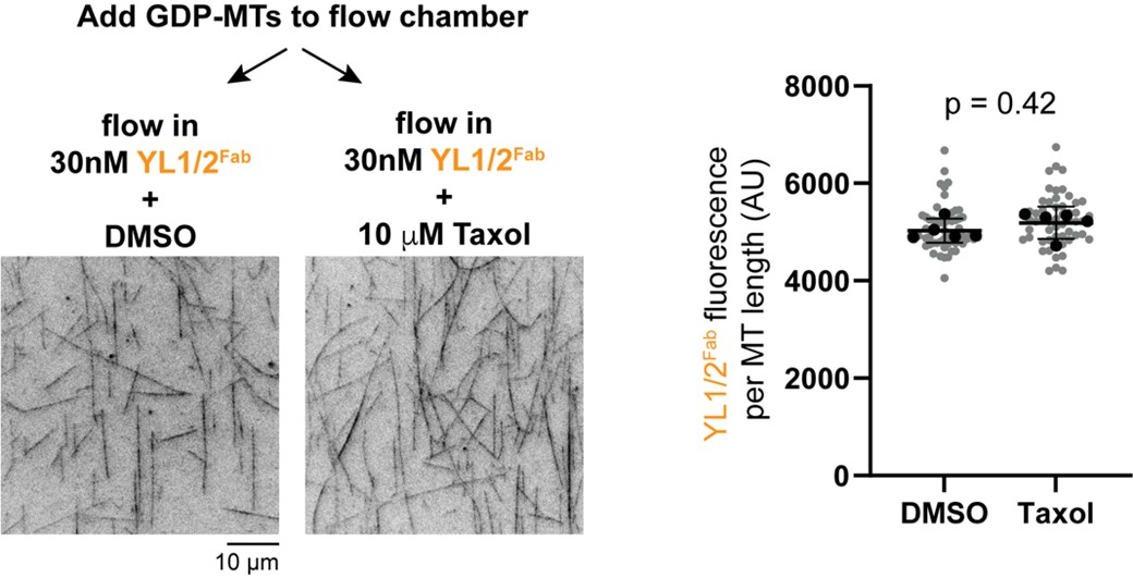
References
Hooikaas, P. J., Martin, M., Muhlethaler, T., Kuijntjes, G. J., Peeters, C. A. E., Katrukha, E. A., Ferrari, L., Stucchi, R., Verhagen, D. G. F., van Riel, W. E., Grigoriev, I., Altelaar, A. F. M., Hoogenraad, C. C., Rudiger, S. G. D., Steinmetz, M. O., Kapitein, L. C. and Akhmanova, A. (2019). MAP7 family proteins regulate kinesin-1 recruitment and activation. J Cell Biol, 218, 1298-1318.
Shen, Y. and Ori-McKenney, K. M. (2024). Microtubule-associated protein MAP7 promotes tubulin posttranslational modifications and cargo transport to enable osmotic adaptation. Dev Cell, 59, 1553-1570.
Tymanskyj, S. R., Yang, B. H., Verhey, K. J. and Ma, L. (2018). MAP7 regulates axon morphogenesis by recruiting kinesin-1 to microtubules and modulating organelle transport. Elife, 7.
Author response:
The following is the authors’ response to the original reviews
Public Reviews:
Reviewer #1 (Public review):
Summary:
This manuscript uses primarily simulation tools to probe the pathway of cholesterol transport with the smoothened (SMO) protein. The pathway to the protein and within SMO is clearly discovered, and interactions deemed important are tested experimentally to validate the model predictions.
Strengths:
The authors have clearly demonstrated how cholesterol might go from the membrane through SMO for the inner and outer leaflets of a symmetrical membrane model. The free energy profiles, structural conformations, and cholesterol-residue interactions are clearly described.
We thank the reviewer for their kind words.
(1) Membrane Model: The authors decided to use a rather simple symmetric membrane with just cholesterol, POPC, and PSM at the same concentration for the inner and outer leaflets. This is not representative of asymmetry known to exist in plasma membranes (SM only in the outer leaflet and more cholesterol in this leaflet). This may also be important to the free energy pathway into SMO. Moreover, PE and anionic lipids are present in the inner leaflet and are ignored. While I am not requesting new simulations, I would suggest that the authors should clearly state that their model does not consider lipid concentration leaflet asymmetry, which might play an important role.
We thank the reviewer for their comment. Membrane asymmetry is inherent in endogenous systems; we acknowledge that as a limitation of our current model. We have addressed the comment by adding this limitation to our discussion in the manuscript.
Added lines: (End of paragraph 6, Results subsection 2):
“One possibility that might alter the thermodynamic barriers is native membrane asymmetry, particularly the anionic lipid-rich inner leaflet. This presents as a limitation of our current model.”
(2) Statistical comparison of barriers: The barriers for pathways 1 and 2 are compared in the text, suggesting that pathway 2 has a slightly higher barrier than pathway 1. However, are these statistically different? If so, the authors should state the p-value. If not, then the text in the manuscript should not state that one pathway is preferred over the other.
We thank the reviewer for their comment. We have added statistical t-tests for the barriers.
Changes made: (Paragraph 6, Results subsection 2)
“However, we also observe that pathway 1 shows a lower thermodynamic barrier (5.8 ± 0.7 kcal/mol v/s 6.5 ± 0.8 kcal/mol, p = 0.0013)”
(3) Barrier of cholesterol (reasoning): The authors on page 7 argue that there is an enthalpy barrier between the membrane and SMO due to the change in environment. However, cholesterol lies in the membrane with its hydroxyl interacting with the hydrophilic part of the membrane and the other parts in the hydrophobic part. How is the SMO surface any different? It has both characteristics and is likely balanced similarly to uptake cholesterol. Unless this can be better quantified, I would suggest that this logic be removed.
We thank the reviewer for this suggestion. We have removed the line to avoid confusion.
Reviewer #2 (Public review):
Summary:
In this work, the authors applied a range of computational methods to probe the translocation of cholesterol through the Smoothened receptor. They test whether cholesterol is more likely to enter the receptor straight from the outer leaflet of the membrane or via a binding pathway in the inner leaflet first. Their data reveal that both pathways are plausible but that the free energy barriers of pathway 1 are lower, suggesting this route is preferable. They also probe the pathway of cholesterol transport from the transmembrane region to the cysteine-rich domain (CRD).
Strengths:
(1) A wide range of computational techniques is used, including potential of mean force calculations, adaptive sampling, dimensionality reduction using tICA, and MSM modelling. These are all applied rigorously, and the data are very convincing. The computational work is an exemplar of a well-carried out study.
(2) The computational predictions are experimentally supported using mutagenesis, with an excellent agreement between their PMF and mRNA fold change data.
(3) The data are described clearly and coherently, with excellent use of figures. They combine their findings into a mechanism for cholesterol transport, which on the whole seems sound.
(4) The methods are described well, and many of their analysis methods have been made available via GitHub, which is an additional strength.
Weaknesses:
(1) Some of the data could be presented a little more clearly. In particular, Figure 7 needs additional annotation to be interpretable. Can the position of the cholesterol be shown on the graph so that we can see the diameter change more clearly?
We thank the reviewer for this suggestion. We have added the cholesterol positions as requested.
Changes made: (Caption, Figure 7)
“The tunnel profile during cholesterol translocation in SMO. (a) Free energy plot of the zcoordinate v/s the tunnel diameter when cholesterol is present in the core TMD. The tunnel shows a spike in the radius in the TMD domain, indicating the presence of a cholesterol-accommodating cavity. (b) Representative figure for the tunnel when a cholesterol molecule is in the TMD. (c) Same as (a), when cholesterol is at the TMD-CRD interface. (e) same as (b), when cholesterol is at the TMD-CRD interface. (e) same as (a), when cholesterol is at the CRD binding site. (f) same as (b), when cholesterol is at the CRD binding site. Tunnel diameters shown as spheres. Cholesterol positions marked on plots using dotted lines. All snapshots presented are frames taken from MD simulations.”
(2) In Figure 3C, it doesn’t look like the Met is constricting the tunnel at all. What residue is constricting the tunnel here? Can we see the Ala and Met panels from the same angle to compare the landscapes? Or does the mutation significantly change the tunnel? Why not A283 to a bulkier residue? Finally, the legend says that the figure shows that cholesterol can still pass this residue, but it doesn’t really show this. Perhaps if the HOLE graph was plotted, we could see the narrowest point of the tunnel and compare it to the size of cholesterol.
We thank the reviewer for this suggestion. A283 was mutated to methionine as it presents with a longer heavy tail containing sulfur. We have plotted the tunnel radii for both WT and A283M mutants and added them as a supplemental figure. As shown in the figure, the presence of methionine doesn’t completely block the tunnel, but occludes it, thereby increasing the barrier for cholesterol transport slightly.
Changes made: (End of Results subsection 1)
“When we calculated the PMF for cholesterol entry, A<sup>2.60f</sup>M mutant showed restricted tunnel but it did not fully block the tunnel (Figure 3—figure Supplement 3).”
(3) The PMF axis in 3b and d confused me for a bit. Looking at the Supplementary data, it’s clear that, e.g., the F455I change increases the energy barrier for chol entering the receptor. But in 3d this is shown as a -ve change, i.e., favourable. This seems the wrong way around for me. Either switch the sign or make this clearer in the legend, please.
We thank the reviewer for this suggestion. We measured ∆PMF as PMF<sub>WT</sub> PMF<sub>mutant</sub>, hence the negative values. We have added additional text to the legend to clarify this.
Changes made: (Caption, Figure 3)
“(b) ∆Gli1 mRNA fold change (high SHH vs untreated) and ∆ PMF (difference of peak PMF , calculated as PMF<sub>WT</sub> - PMF<sub>mutant</sub>) plotted for the mutants in Pathway 1. (c) Example mutant A<sup>2_._60f</sup>M shows that cholesterol can enter SMO through Pathway 1 even on a bulky mutation. (d) Same as (b) but for Pathway 2 (e) Example mutant L<sup>5.62f</sup>A shows that cholesterol can enter SMO through Pathway 2 due to lesser steric hindrance. All snapshots presented are frames taken from MD simulations.”
Changes made: (Caption, Figure 6)
“(b) ∆Gli1 mRNA fold change (high SHH vs untreated) and ∆ PMF (difference of peak PMF, calculated as PMF<sub>WT</sub> - PMF<sub>mutant</sub>) plotted for mutants along the TMD-CRD pathway. (c, d) Example mutants Y<sup>LD</sup>A and F<sup>5.65f</sup>A show that cholesterol is unable to translocate through this pathway because of the loss of crucial hydrophobic contacts provided by Y207 and F484 and along the solvent-exposed pathway.”
(4) The impact of G280V is put down to a decrease in flexibility, but it could also be a steric hindrance. This should be discussed.
We thank the reviewer for this suggestion. We have added it as a possible mechanism of the decrease in activity of SMO.
Changes made: (Paragraph 5, Results subsection 1)
“We mutated G280<sup>2.57f</sup> to valine - G<sup>2.57f</sup>V to test whether reducing the flexibility of TM2 prevents cholesterol entry into the TMD. Consequently, the activity of mSMO showed a decrease. However, this decrease could also be attributed to steric hindrance added by the presence of a bulky propyl group in valine.”
(5) Are the reported energy barriers of the two pathways (5.8plus minus0.7 and 6.5plus minus0.8 kcal/mol) significantly and/or substantially different enough to favour one over the other? This could be discussed in the manuscript.
We thank the reviewer for this suggestion. We have added statistical t-tests for the barriers.
Changes made: (Paragraph 6, Results subsection 2)
“However, we also observe that pathway 1 shows a lower thermodynamic barrier (5.8 ± 0.7 kcal/mol v/s 6.5 ± 0.8 kcal/mol, p = 0.001)”
(6) Are the energy barriers consistent with a passive diffusion-driven process? It feels like, without a source of free energy input (e.g., ion or ATP), these barriers would be difficult to overcome. This could be discussed.
We thank the reviewer for this suggestion. We have added a discussion to further clarify this point.
Discussion: (Paragraph 6, Results subsection 2)
“These values are comparable to ATP-Binding Cassette (ABC) transporters of membrane lipids, which use ATP hydrolysis (-7.54 ± 0.3 kcal/mol) (Meurer et al., 2017) to drive lipid transport from the membrane to an extracellular acceptor. Some of these transporters share the same mechanism as SMO, where the lipid from the inner leaflet is flipped and transported to the extracellular acceptor protein (Tarling et al., 2013). Additionally, for secondary active transporters that do not use ATP for the transport of substrates, a thermodynamic barrier of 5-6 kcal/mol has been reported in literature. (Chan et al., 2022; Selvam et al., 2019; McComas et al., 2023; Thangapandian et al., 2025).”
(7) Regarding the kinetics from MSM, it is stated that the values seen here are similar to MFS transporters, but this then references another MSM study. A comparison to experimental values would support this section a lot.
We thank the reviewer for this suggestion. We have added a discussion discussing millisecond-scale timescales measured for MFS transporters.
Changes made: (Paragraph 2, Results subsection 5)
“These timescales are comparable to the substrate transport timescales of Major Facilitator Superfamily (MFS) transporters (Chan et al., 2022). Furthermore, several experimental studies have also resolved the millisecond-scale kinetics of MFS transporters (Blodgett and Carruthers, 2005; Körner et al., 2024; Bazzone et al., 2022; Smirnova et al., 2014; Zhu et al., 2019), further corroborating the results from our study.”
Reviewer #2 (Recommendations for the authors):
(1) The heatmaps in Figures 2a and 4a are great. On these, an arrow denotes what looks like a minimum energy path. Is it possible to see this plotted, as this might show the height of the energy barriers more clearly?
We thank the reviewer for this suggestion. We have computed the minimum energy paths for both pathways and presented them in a supplementary figure.
Added lines: (Paragraph 4, Results subsection 1):
For further clarity, we have plotted the minimum energy path taken by cholesterol as it translocates along this pathway (Figure 2—figure Supplement 3)a,b)
Added lines: (Paragraph 4, Results subsection 2):
For further clarity, we have plotted the minimum energy path taken by cholesterol as it translocates along this pathway (Figure 2—figure Supplement 3)c,d)
(2) The tiCA data in S15 is first referred to on line 137, but the technique isn’t introduced until line 222. This makes understanding the data a little confusing. Reordering this might improve readability.
We thank the reviewer for this suggestion. We have reordered the text to make it clearer.
Changes made: (Paragraph 2, Results subsection 1) This provides evidence for multiple stable poses along the pathway as observed in the multiple stable poses of cholesterol in Cryo-EM structures of SMO bound to sterols (Deshpande et al., 2019; Qi et al., 2019b, 2020). A reliable estimate of the barriers comes from using the time-lagged Independent Components (tICs), which project the entire dataset along the slowest kinetic degrees of freedom. Overall, the highest barrier along Pathway 1 is ∼ 5.8 ± 0.7 kcal/mol, and it is associated with the entry of cholesterol into the TMD (Figure 2—Figure Supplement 2).
Changes made: (Paragraph 3, Results subsection 2)
“On plotting the first two components of tICs, (Figure 2—Figure Supplement 2), we observe that the energetic barrier between η and θ is ∼6.5 ± 0.8 kcal/mol.”
(3) Missing bracket on line 577.
We thank the reviewer for this suggestion. The typo has been fixed.
(4) Line 577: Fig. S2nd?
We thank the reviewer for this suggestion. This typo has been fixed.
Reviewer #3 (Public review):
Summary:
This manuscript presents a study combining molecular dynamics simulations and Hedgehog (Hh) pathway assays to investigate cholesterol translocation pathways to Smoothened (SMO), a G protein-coupled receptor central to Hedgehog signal transduction. The authors identify and characterize two putative cholesterol access routes to the transmembrane domain (TMD) of SMO and propose a model whereby cholesterol traverses through the TMD to the cysteine-rich domain (CRD), which is presented as the primary site of SMO activation. The MD simulations and biochemical experiments are carefully executed and provide useful data.
Weaknesses:
However, the manuscript is significantly weakened by a narrow and selective interpretation of the literature, overstatement of certain conclusions, and a lack of appropriate engagement with alternative models that are well-supported by published data-including data from prior work by several of the coauthors of this manuscript. In its current form, the manuscript gives a biased impression of the field and overemphasizes the role of the CRD in cholesterol-mediated SMO activation. Below, I provide specific points where revisions are needed to ensure a more accurate and comprehensive treatment of the biology.
(1) Overstatement of the CRD as the Orthosteric Site of SMO Activation
The manuscript repeatedly implies or states that the CRD is the orthosteric site of SMO activation, without adequate acknowledgment of alternative models. To give just a few examples (of many in this manuscript):
(a) “PTCH is proposed to modulate the Hh signal by decreasing the ability of membrane cholesterol to access SMO’s extracellular cysteine-rich domain (CRD)” (p. 3).
(b) “In recent years, there has been a vigorous debate on the orthosteric site of SMO” (p. 3).
(c) “cholesterol must travel through the SMO TMD to reach the orthosteric site in the CRD” (p. 4).
(d) “we observe cholesterol moving along TM6 to the TMD-CRD interface (common pathway, Fig. 1d) to access the orthosteric binding site in the CRD” (p. 6).
While the second quote in this list at least acknowledges a debate, the surrounding text suggests that this debate has been entirely resolved in favor of the CRD model. This is misleading and not reflective of the views of other investigators in the field (see, for example, a recent comprehensive review from Zhang and Beachy, Nature Reviews Molecular and Cell Biology 2023, which makes the point that both the CRD and 7TM sites are critical for cholesterol activation of SMO as well as PTCH-mediated regulation of SMO-cholesterol interactions).
In contrast, a large body of literature supports a dual-site model in which both the CRD and the TMD are bona fide cholesterol-binding sites essential for SMO activation. Examples include:
(a) Byrne et al., Nature 2016: point mutation of the CRD cholesterol binding site impairs-but does not abolish-SMO activation by cholesterol (SMO D99A, Y134F, and combination mutants - Fig 3 of the 2016 study).
(b) Myers et al., Dev Cell 2013 and PNAS 2017: CRD deletion mutants retain responsiveness to PTCH regulation and cholesterol mimetics (similar Hh responsiveness of a CRD deletion mutant is also observed in Fig. 4 Byrne et al, Nature 2016).
(c) Deshpande et al., Nature 2019: mutation of residues in the TMD cholesterol binding site blocks SMO activation entirely, strongly implicating the TMD as a required site, in contrast to the partial effects of mutating or deleting the CRD site.
Qi et al., Nature 2019, and Deshpande et al., Nature 2019, both reported cholesterol binding at the TMD site based on high-resolution structural data. Oddly, Deshpande et al., Nature 2019, is not cited in the discussion of TMD binding on p. 3, despite being one of the first papers to describe cholesterol in the TMD site and its necessity for activation (the authors only cite it regarding activation of SMO by synthetic small molecules).
Kinnebrew et al., Sci Adv 2022 report that CRD deletion abolished PTCH regulation, which is seemingly at odds with several studies above (e.g., Byrne et al, Nature 2016; Myers et al, Dev Cell 2013); but this difference may reflect the use of an N-terminal GFP fusion to SMO in the Kinnebrew et al 2022, which could alter SMO activation properties by sterically hindering activation at the TMD site by cholesterol (but not synthetic SMO agonists like SAG); in contrast, the earlier work by Byrne et al is not subject to this caveat because it used an untagged, unmodified form of SMO.
Although overexpression of PTCH1 and SMO (wild-type or mutant) has been noted as a caveat in studies of CRD-independent SMO activation by cholesterol, this reviewer points out that several of the studies listed above include experiments with endogenous PTCH1 and low-level SMO expression, demonstrating that SMO can clearly undergo activation by cholesterol (as well as regulation by PTCH1) in a manner that does not require the CRD.
Recommendation: The authors should revise the manuscript to provide a more balanced overview of the field and explicitly acknowledge that the CRD is not the sole activation site. Instead, a dual-site model is more consistent with available structural, mutational, and functional data. In addition, the authors should reframe their interpretation of their MD studies to reflect this broader and more accurate view of how cholesterol binds and activates SMO.
We thank the reviewer for this comprehensive overview of the existing literature. We agree that cholesterol binding to both the TMD and CRD sites is required for full activation of SMO. As described below in responses to comments, we have made changes to the manuscript to make this point clear. For instance, in the revised manuscript, we refrain from calling the CRD cholesterol binding site the “orthosteric site”. Instead, we highlight that the goal of the manuscript is not to resolve the debate over whether the TMD or CRD site is more important for PTCH1 regulation by SMO but rather to use molecular dynamics to understand the fascinating question of how cholesterol in the membrane can reach the CRD, located at a significant distance above the outer leaflet of the membrane. We believe that this is an important goal since there is an abundance of evidence that supports the view that PTCH1 inhibits SMO by reducing cholesterol access to the CRD. This evidence is now summarized succinctly in the introduction:
Changes made: (Paragraph 4, Introduction)
“While cholesterol binding to both the TMD and CRD sites is required for full SMO activation, our work focuses on how cholesterol gains access to the CRD site, perched above the outer leaflet of the membrane (Luchetti et al., 2016; Kinnebrew et al., 2022). Multiple lines of evidence suggest that PTCH1-regulated cholesterol binding to the CRD plays an instructive role in SMO regulation both in cells and animals. Mutations in residues predicted to make hydrogen bonds with the hydroxyl group of cholesterol bound to the CRD reduced both the potency and efficacy of SHH in cellular signaling assays (Kinnebrew et al., 2022; Byrne et al., 2016) and, more importantly, eliminated HH signaling in mouse embryos (Xiao et al., 2017). Experiments using both covalent and photocrosslinkable sterol probes in live cells directly show that PTCH1 activity reduces sterol access to the CRD (Kinnebrew et al., 2022; Xiao et al., 2017). Notably, our simulations evaluate a path of cholesterol translocation that includes both the TMD and CRD sites: cholesterol first enters the 7-transmembrane domain bundle from the membrane; it then engages the TMD site before continuing along a conduit to the CRD site. Thus, we analyze translocation energetics and residue-level contacts along a path that includes both the TMD and the CRD.”
However, Reviewer 3 makes several comments below that are biased, inaccurate, or selective. We feel it is important to address these so readers can approach the literature from a balanced perspective. Indeed, the eLife review forum provides an ideal venue to present contrasting views on a scientific model. We encourage the editors to publish both Reviewer 3’s comments and our response in full so readers can read the original papers and reach their own conclusions. It is important to note these issues are not relevant to the quality of the computational and experimental data presented in this paper.
We have now removed the term “orthosteric” to describe the CRD site throughout the paper and clearly state in the introduction that “both the CRD and TMD sites are required for SMO activation” but that our focus is on how cholesterol moves from the membrane to the CRD site. There is no doubt that cholesterol binding to the CRD plays a key role in SMO activation– our focus on this path is justified and does not devalue the importance of the TMD site. Our prior models (see Figure 7 of Kinnebrew 2022 explicitly include contributions of both sites).
Now we respond to some of the concerns outlined, individually:
(1) Byrne et al., Nature 2016: point mutation of the CRD cholesterol binding site impairs-but does not abolish-SMO activation by cholesterol (SMO D99A, Y134F, and combination mutants - Fig 3 of the 2016 study)
The fact that a point mutation dramatically diminishes (but does not abolish signaling) does not mean that the CRD cholesterol binding site is not important for SMO regulation. Indeed, the reviewer fails to mention that Song et. al. (Molecular Cell, 2017) found that a SMO protein carrying a subtle mutation at D99 (D95/99N, a residue that makes a hydrogen bond with the cholesterol hydroxyl) completely abolishes SMO signaling in mouse embryos. Thus, the CRD site is critical for SMO activation in an intact animal, justifying our focus on evaluating the path of cholesterol translocation to the CRD site.
(2) Myers et al., Dev Cell 2013 and PNAS 2017: CRD deletion mutants retain responsiveness to PTCH regulation and cholesterol mimetics (similar Hh responsiveness of a CRD deletion mutant is also observed in Fig 4 Byrne et al, Nature 2016).
The Reviewer fails to note that CRD-deleted versions of SMO have markedly (>10-fold) higher basal (i.e. ligand-independent) activity compared to full-length SMO. The response to SHH is minimal (∼2-fold), compared to >50-100-fold with full-length SMO. Thus, CRD-deleted SMO is likely in a non-native conformation. Local changes in cholesterol accessibility caused by PTCH1 inactivation or cholesterol loading can cause small fluctuations in delta-CRD activity, but this cannot be used to infer meaningful insights about how native, full-length SMO (with >10-fold lower basal activity) is regulated. We encourage the reviewer to read our previous paper (Kinnebrew et. al. 2022), which presents a unified view of how the TMD and CRD sites together regulate SMO activation.
A more physiological experiment, reported in Kinnebrew et. al. 2022, tested mutations in residues that make hydrogen bonds with cholesterol at the CRD and TMD sites in the context of full-length SMO. These mutants were stably expressed at moderate levels in Smo<sup>−/−</sup> cells. Mutations at the CRD site reduced the fold-increase in signaling output in response to SHH, as would be expected for a PTCH1-regulated site. In contrast, analogous mutations in the TMD site reduced the magnitude of both basal and maximal signaling, without affecting the fold-change in response to SHH. In signaling assays, the key parameter in evaluating the impact of a mutation is whether it impacts the change in output in response to a signal (in this case PTCH1 inactivation by SHH). A mutation in SMO that affects PTCH1 regulation is expected to decrease the fold-change in signaling in response to SHH, a criterion that is fulfilled by mutations in the CRD site. Accordingly, mutations in the CRD site abolish SMO signaling in mouse embryos (Xiao et al., 2017).
(3) Deshpande et al., Nature 2019: mutation of residues in the TMD cholesterol binding site blocks SMO activation entirely, strongly implicating the TMD as a required site, in contrast to the partial effects of mutating or deleting the CRD site.
Introduction of bulky mutations at the TMD site (V333F) that abolish SMO activity were first reported by Byrne et. al. 2016 and were used to markedly increase the stability of SMO for protein expression. These mutations indeed stabilize the inactive state of SMO, increasing protein abundance and completely preventing its localization at primary cilia. SMO variants carrying such bulky mutations cannot be used to infer the importance of the TMD site since they do not distinguish between the following possibilities: (1) SMO is inactive because the sterol cannot bind, or (2) SMO is inactive because it is locked in an inactive conformation, or (3) SMO is inactive because it cannot localize to primary cilia (where it must be localized to activate downstream signaling).
As described in Response 3.3, a better evaluation of the importance of the TMD site is the use of mutations in residues that make hydrogen bonds with the hydroxyl group of TMD cholesterol. These mutations do not markedly increase protein stability or prevent ciliary localization (Kinnebrew 2022, Fig.S2). While a TMD site mutation decreases the magnitude of maximal (and basal) SMO signaling, it does not impact the fold-increase in signal output in response to Hh ligands (the key parameter that should be used to evaluate PTCH1 activity).
(4) Qi et al., Nature 2019, and Deshpande et al., Nature 2019, both reported cholesterol binding at the TMD site based on high-resolution structural data. Oddly, Deshpande et al., Nature 2019 not cited in the discussion of TMD binding on p. 3, despite being one of the first papers to describe cholesterol in the TMD site and its necessity for activation (the authors only cite it regarding activation of SMO by synthetic small molecules)
The reference has now been added at this location in the manuscript.
(5) Kinnebrew et al., Sci Adv 2022 report that CRD deletion abolished PTCH regulation, which is seemingly at odds with several studies above (e.g., Byrne et al, Nature 2016; Myers et al, Dev Cell 2013); but this difference may reflect the use of an N-terminal GFP fusion to SMO in the Kinnebrew et al 2022, which could alter SMO activation properties by sterically hindering activation at the TMD site by cholesterol (but not synthetic SMO agonists like SAG); in contrast, the earlier work by Byrne et al is not subject to this caveat because it used an untagged, unmodified form of SMO.
The reviewer fails to note that CRD deleted versions of SMO have markedly (>10-fold) higher basal activity than full-length SMO. The response to SHH is minimal (∼2fold), compared to >50-fold with full-length SMO. Thus, CRD-deleted SMO is likely in a non-native conformation. Local changes in cholesterol accessibility caused by PTCH1 inactivation or cholesterol loading can cause small fluctuations in delta-CRD activity, but this cannot be used to infer meaningful insights about how native, full-length SMO (with >10-fold lower basal activity) is regulated. Please see Response 3.3 for further details.
Reviewer 3 presents an incomplete picture of the extensive experiments reported in Kinnebrew et. al. to establish the functionality of YFP-tagged delta-CRD SMO. Most importantly, a TMDselective sterol analog (KK174) can fully activate YFP-tagged delta-CRD, showing conclusively that the YFP fusion does not block sterol access to the TMD site. The fact that this protein is nearly unresponsive to SHH highlights the critical role of the CRD-bound cholesterol in SMO regulation by PTCH1. Indeed, the YFP-tagged, CRD-deleted SMO was made purposefully to test the requirement of the CRD in a construct that had normal basal activity. Again, this data justifies the value of investigating the path of cholesterol movement from the membrane via the TMD site to the CRD.
(6) Although overexpression of PTCH1 and SMO (wild-type or mutant) has been noted as a caveat in studies of CRD-independent SMO activation by cholesterol, this reviewer points out that several of the studies listed above include experiments with endogenous PTCH1 and low-level SMO expression, demonstrating that SMO can clearly undergo activation by cholesterol (as well as regulation by PTCH1) in a manner that does not require the CRD.
This comment is inaccurate. The data presented in Deshpande et. al. (and prior work in Myers et. al.) used transient transfection to overexpress SMO in Smo<sup>−/−</sup> cells. At the individual cell level transient transfection produces expression levels that are markedly higher (10-1000-fold) than stable expression (in addition to being more variable). Most scientists would agree that stable expression (as used in Kinnebrew 2022) at a moderate expression level is a better system to compare mutant phenotypes, assess basal and activated signaling, and provide an accurate measure of the fold-change in signal output in response to SHH. Notably, introduction of a mutation in the CRD cholesterol binding site at the endogenous mouse Smo locus (an even better experiment than stable expression) leads to complete loss of SMO activity (PMID 28344083). This result again justifies our investigation of the pathway of cholesterol movement from the membrane to the CRD site.
We have changed the initial discussion and reflect a more general outlook.
Changes made: (Paragraph 1, Introduction)
“PTCH modulates the availability of accessible cholesterol at the primary cilium and thereby regulates SMO, with models invoking effects on both the CRD and 7TM pockets.”
Changes made: (Results subsection 3, paragraph 1)
“According to the dual-site model, to reach the binding site in the CRD (ζ), cholesterol translocate along the TMD-CRD interface from the TM binding site (α∗) is required.”
Added lines: (Paragraph 5, Results subsection 3):
“The computational investigation showed here covers the dual-site model, where cholesterol reaches the CRD site via binding to the TM binding site first. In comparison to the CRD site, the TM site is more stable by ∼ 2 kcal/mol (Figure 2—Figure Supplement 3b, d).”
Added lines: (Paragraph 2, Conclusions):
“Here we have explored the role the CRD-site plays in SMO activation. In addition, through simulating the CRD site-dependent SMO activation hypothesis, we have also simulated the TMD site-dependent activation. We show that the overall stability of cholesterol is higher than the CRD site by ∼ 2 kcal/mol.”
(2) Bias in Presentation of Translocation Pathways
The manuscript presents the model of cholesterol translocation through SMO to the CRD as the predominant (if not sole) mechanism of activation. Statements such as: "Cholesterol traverses SMO to ultimately reach the CRD binding site" (p. 6) suggest an exclusivity that is not supported by prior literature in the field. Indeed, the authors’ own MD data presented here demonstrate more stable cholesterol binding at the TMD than at the CRD (p 17), and binding of cholesterol to the TMD site is essential for SMO activation. As such, it is appropriate to acknowledge that cholesterol may activate SMO by translocating through the TM5/6 tunnel, then binding to the TMD site, as this is a likely route of SMO activation in addition to the CRD translocation route they highlight in their discussion.
The authors describe two possible translocation pathways (Pathway 1: TM2/3 entry to TMD; Pathway 2: TM5/6 entry and direct CRD transfer), but do not sufficiently acknowledge that their own empirical data support Pathway 2 as more relevant. Indeed, because their experimental data suggest Pathway 2 is more strongly linked to SMO activation, this pathway should be weighted more heavily in the authors’ discussion. In addition, Pathway 2 is linked to cholesterol binding to both the TMD and CRD sites (the former because the TMD binding site is at the terminus of the hydrophobic tunnel, the latter via the translocation pathway described in the present manuscript), so it is appropriate that Pathway 2 figures more prominently than Pathway 1 in the authors’ discussion.
The authors also claim that "there is no experimental structure with cholesterol in the inner leaflet region of SMO TMD" (p 16). However, a structural study of apo-SMO from the Manglik and Cheng labs (Zhang et al., Nat Comm, 2022) identified a cholesterol molecule docked at the TM5/6 interface and also proposed a "squeezing" mechanism by which cholesterol could enter the TM5/6 pocket from the membrane. The authors do not consider this SMO conformation in their models, nor do they discuss the possibility that conformational dynamics at the TM5/6 interface could facilitate cholesterol flipping and translocation into the hydrophobic conduit, despite both possibilities having precedent in the 2022 empirical cryoEM structural analysis.
Recommendation: The authors should avoid oversimplifying the SMO cholesterol activation process, either by tempering these claims or broadening their discussion to better reflect the complexity and multiplicity of cholesterol access and activation routes for SMO. They should also consider the 2022 apo-SMO cryoEM structure in their analysis of the TM5/6 translocation pathway.
We thank the reviewer for this comprehensive overview of the existing literature and parts we have missed to include in the discussion. We agree with the reviewer, since our data shows that both pathways are probable. Through our manuscript, we have avoided using a competitive approach (that one pathway dominates over the other). Instead, we have evaluated both pathways independently and presented a comparative rather than competitive overview of both pathways from our observations. While we agree that experimental evidence suggests the inner leaflet pathway is possible, we cannot discount the observations made in previous studies that support the outer leaflet pathway, particularly Hedger et al. (2019), Bansal et al. (2023), and Kinnebrew et al. (2021). Therefore, considering the reviewer’s comments have made the following changes:
(1) Added lines: (Paragraph 3, Conclusions):
“We show that the barriers associated with the pathway starting from the outer leaflet are lower by ∼0.7 kcal, (p=0.0013). We also provide evidence that cholesterol can enter SMO via both leaflets, considering that multiple computational and experimental studies have found cholesterol entry sites and activation modulation via the outer leaflet, between TM2TM3. This is countered by evidence from multiple experimental and computational studies corroborating entry via the inner leaflet, between TM5-TM6, including this study. Overall, we posit that cholesterol translocation from either pathway is feasible.”
(2)nChanges made: (Paragraph 6, Results subsection 2)
“Based on our experimental and computational data, we conclude that cholesterol translocation can happen via either pathway. This is supported on the basis of the following observations: mutations along pathway 2 affect SMO activity more significantly, and the presence of a direct conduit that connects the inner leaflet to the TMD binding site. In addition, a resolved structure of SMO in the presence of cholesterol shows a cholesterol situated at the entry point from the membrane into the protein between TM5 and TM6, in the inner leaflet. However, we also observe that pathway 1 shows a lower thermodynamic barrier (5.8 ± 0.7 kcal/mol vs. 6.5 ± 0.8 kcal/mol, p \= 0.0013). Additionally, PTCH1 controls cholesterol accessibility in the outer leaflet. This shows that there is a possibility for transport from both leaflets. One possibility that might alter the thermodynamic barriers is native membrane asymmetry, particularly the anionic lipid-rich inner leaflet. This presents as a limitation of our current model.”
(3)nChanges made: (Paragraph 1, Results subsection 2)
“In a structure resolved in 2022, cholesterol was observed at the interface between the protein and the membrane, in the inner leaflet, between TMs 5 and 6. However, cholesterol in the inner leaflet has a downward orientation, with the polar hydroxyl group pointing intracellularly (η). A striking observation is that this cholesterol binding site pose was never used as a starting point for simulations and was discovered independent of the pose described in Zhang et al. (2022) (Figure 4—Figure Supplement 1).”
(3) Alternative Possibility: Direct Membrane Access to CRD
The possibility that the CRD extracts cholesterol directly from the membrane outer leaflet is not considered. While the crystal structures place the CRD in a stable pose above the membrane, multiple cryo-EM studies suggest that the CRD is dynamic and adopts a variety of conformations, raising the possibility that the stability of the CRD in the crystal structures is a result of crystal packing and that the CRD may be far more dynamic under more physiological conditions.
Recommendation: The authors should explicitly acknowledge and evaluate this potential mechanism and, if feasible, assess its plausibility through MD simulations.
We thank the reviewer for the suggestion. We have addressed this comment by calculating the distance from the lipid headgroups for each lipid in the membrane to the cholesterol binding site. We show that in our study, we do not observe any bending of the CRD over the membrane, precluding any cholesterol from being extracted from the membrane directly.
Added lines: (Paragraph 3, Conclusions):
“An alternative possibility states that the flexibility associated with the CRD would allow it to directly access the membrane, and consequently, cholesterol. In the extensive simulations reported in this study, the binding site of cholesterol in the CRD remains at least 20 Å away from the nearest lipid head group in the membrane, suggesting that such direct extraction and the bending of the CRD do not occur within the timescales sampled (Appendix 2 – Figure 6).
The mechanistic details of this process are still unexplored and form the basis of future work.”
(4) Inconsistent Framing of Study Scope and Limitations
The discussion contains some contradictory and misleading language. For example, the authors state that "In this study we only focused on the cholesterol movement from the membrane to the CRD binding site," and then several sentences later state that "We outline the entire translocation mechanism from a kinetic and thermodynamic perspective." These statements are at odds. The former appropriately (albeit briefly) notes the limited scope of the modeling, while the latter overstates the generality of the findings.
In addition, the authors’ narrow focus on the CRD site constitutes a major caveat to the entire work. It should be acknowledged much earlier in the manuscript, preferably in the introduction, rather than mentioned as an aside in the penultimate paragraph of the conclusion.
Recommendation: The authors should clarify the scope of the study and expand the discussion of its limitations. They should explicitly acknowledge that the study models one of several cholesterol access routes and that the findings do not rule out alternative pathways.
We thank the reviewer for the suggestion. We have addressed this comment by explicitly mentioning the scope of the study.
Changes made: (Paragraph 3, Conclusions)
“We outline the entire translocation mechanism from a kinetic and thermodynamic perspective for one of the leading hypotheses for the activation mechanism of SMO.”
(5) Summary:
This study has the potential to make a useful contribution to our understanding of cholesterol translocation and SMO activation. However, in its current form, the manuscript presents an overly narrow and, at times, misleading view of the literature and biological models; as such, it is not nearly as impactful as it could be. I strongly encourage the authors to revise the manuscript to include:
(1) A more balanced discussion of the CRD vs. TMD binding sites.
(2) Acknowledgment of alternative cholesterol access pathways.
(3) More comprehensive citation of prior structural and functional studies.
(4) Clarification of assumptions and scope.
Of note, the above suggestions require little to no additional MD simulations or experimental studies, but would significantly enhance the rigor and impact of the work.
We thank the reviewer for the suggestions. We have taken into account the literature and diverse viewpoints. We have changed the initial discussion and reflected a more general outlook. In the revised version of the manuscript, we have refrained from referring to the CRD site as the orthosteric site. Instead, we refer to it as the CRD sterol-binding site. To better represent the dual-site model, we add further discussion in the Introduction. Through our manuscript, we have avoided using a competitive approach (that one pathway dominates over the other). Instead, we have evaluated both pathways independently and presented a comparative rather than competitive overview of both pathways from our observations. We explicitly mention the scope of the study.
Author response:
Public Reviews:
Reviewer #1 (Public review):
The author presents a new method for microRNA target prediction based on (1) a publicly available pretrained Sentence-BERT language model that the author fine-tunes using MeSH information and (2) downstream classification analysis for microRNA target prediction. In particular, the author's approach, named "miRTarDS", attempts to solve the microRNA target prediction problem by utilizing disease information (i.e., semantic similarity scores) from their language model. The author then compares the prediction performance with other sequence- and disease-based methods and attempts to show that miRTarDS is superior or at least comparable to existing methods. The author's general approach to this microRNA target prediction problem seems promising, but fails to demonstrate concrete computational evidence that miRTarDS outperforms other existing methods. The author's claim that disease information-based language models are sufficient is unfounded. The manuscript requires substantial rewriting and reorganization for readers with a strong background in biomedical research.
We appreciate the reviewer’s careful examination of modeling, benchmarking, and interpretation, and we are particularly encouraged that they found the proposed method promising. We will make corresponding revisions to the manuscript based on the reviewer’s comments.
A major issue related to the author's claim of computational advance of miRTarDS: The author does not introduce existing biomedical-specific language models, and does not compare them against miRTarDS's fine-tuned model. The performance of miRTarDS is largely dependent on the semantic embedding of disease terms. The author shows in Figure 5 that MeSH-based fine-tuning leads to a substantial improvement in MeSH-based correlation compared to the publicly available pretrained SBERT model "multi-qa-MiniLM-L6-cos-v1" without sacrificing a large amount of BIOSSES-based correlation. However, the author does not compare the performance of MeSH- and BIOSSES-based correlation with existing language models such as ChatGPT, BioBERT, PubMedBERT, and more. Also, the substantial improvement in MeSH-based correlation is a mere indication that the MeSH-based fine-tuning strategy was reasonable and not that it's superior to the publicly available pretrained SBERT model "multi-qa-MiniLM-L6-cos-v1".
We thank the reviewer for the constructive suggestions regarding the benchmarking of language models. We acknowledge that the performance of miRTarDS largely depends on the semantic embeddings of disease terms. So, in the revisions, I will: 1) conduct a literature review to introduce existing biomedical-specific language models, and 2) perform a horizontal comparison between our fine-tuned model and these existing models, to more comprehensively evaluate the model’s capabilities.
Another major issue is in the author's claim that disease-information from miRTarDS's language model is "sufficient" for accurate microRNA target prediction. Available microRNA targets with experimental evidence are largely biased for those with disease implications that have been reported in the biomedical literature. It's possible that their language model is biased by existing literature that has also been used to build microRNA target databases. Therefore, it is important that the author provides strong evidence that excludes the possibility of data leakage circularity. Similar concerns are prevalent across the manuscript, and so I highly recommend that the author reassess the evaluation frameworks and account for inflated performance, biased conclusions, and self-confirming results.
We thank the reviewer for the comment. We recognize that existing experimentally validated microRNA targets may be biased toward those reported in biomedical literature as disease‑related. To mitigate this bias, we attempted to extract predicted microRNA targets that share a very similar number of miRNA- and gene‑ disease entries as the experimentally validated microRNA targets using the K‑Nearest Neighbors (KNN) method. Then applied Positive‑Unlabeled (PU) Learning to classify the two groups. PU‑Learning is designed to address scenarios where only a subset of the training data is explicitly labeled as positive, while the remaining data are unlabeled—with the unlabeled set containing both potential positives and true negatives—which is highly suitable for the application context of this manuscript [1]. Preliminary results show that after applying the new data extraction and classification approach, model performance drops to around F1=0.73 (the MISIM method also shows a decline, with F1 around 0.58; detailed code is available on GitHub). The specific reasons for this require further investigation.
Last but not least, the manuscript requires a deeper and careful description and computational encoding of microRNA biology. I'd advise the author to include an expert in microRNA biology to improve the quality of this manuscript. For example, the author uses the pre-miRNA notation and replaces the mature miRNA notation to maintain computational encoding consistency across databases. However, the mature microRNA notation "the '-3p' or '-5p' is critical as the 3p and 5p mature microRNAs have different seed sequences and thus different mRNA targets. The 3p mature microRNA would most likely not target an mRNA targeted by the 5p mature microRNA.
We thank the reviewer for the critique and suggestion. We fully agree with the reviewer that the distinction between the 3p and 5p mature strands is critical for determining mRNA targeting, as they possess distinct seed sequences. In our study, we relied on the miRNA–disease associations provided by the HMDD database, which annotates interactions at the pre-miRNA level: “… the enriched functions of each mature miRNA are aggregated to the corresponding miRNA precursor.” [2] Furthermore, existing literature suggests that the pre-miRNA level can be appropriate and informative for disease association analyses: “Compared with the mature miRNA method, the pre-miRNA method is more useful for studying disease association.” [3] We also find that, in some cases, both strands cooperate to regulate the same or complementary pathways [4]. We acknowledge the reviewer’s point as an important consideration for future revision. We plan to consult or collaborate with biologists to enhance the quality of the manuscript in biology.
Reviewer #2 (Public review):
This study introduces a novel knowledge-driven approach, miRTarDS, which enables microRNA-Target Interaction (MTI) prediction by leveraging the disease association degree between a miRNA and its target gene. The core hypothesis is that this single feature is sufficient to distinguish experimentally validated functional MTIs from computationally predicted MTIs in a binary classification setting. To quantify the disease association, the authors fine-tuned a Sentence-BERT (SBERT) model to generate embeddings of disease descriptions and compute their semantic similarity. Using only this disease association feature, miRTarDS achieved an F1 score of 0.88 on the test set.
We thank the reviewers for their positive feedback, especially for their recognition of the novelty of this manuscript.
Strengths:
The primary strength is the innovative use of the disease association degree as an independent feature for MTI classification. In addition, this study successfully adapts and fine-tunes the Sentence-BERT (SBERT) model to quantify the semantic similarity between biomedical texts (disease descriptions). This approach establishes a critical pathway for integrating powerful language models and the vast growth in clinical/disease data into biochemical discovery, like MTI prediction.
We would like to thank the reviewer again for their positive feedback. We appreciate their recognition of the novelty of our work, as well as their acknowledgment that the proposed method paves the way for integrating language models with clinical/disease data into biochemical discovery.
Weaknesses:
The main weakness lies in its definition of the ground-truth dataset, which serves as a foundation for methodological evaluation. The study defines the Negative Set as computationally predicted MTIs that lack experimental evidence. However, the absence of experimental validation does not equate to non-functionality. Similarly, the miRAW sets are classified by whether the target and miRNA could form a stable duplex structure according to RNA structure prediction. This definition is biologically irrelevant, as duplex stability does not fully encapsulate the complex in vivo binding of miRNAs within the AGO protein complex.
We thank the reviewers for their constructive feedback. We have realized that treating predicted MTI as a negative class may pose some issues. Therefore, we have decided to adopt Positive Unlabeled (PU) Learning in subsequent updates. This classification method can be applied to datasets such as ours, which contain only positive classes and lack negative ones [1]. We used the miRAW dataset to enable a horizontal comparison of our method with traditional sequence-based prediction approaches. We acknowledge that miRAW may overlook some biological insights, and we plan to optimize the construction of test datasets in the future. Some preliminary explorations have already been conducted, and the relevant code is available on GitHub.
Furthermore, we will make the following revisions: 1) We will clearly specify the version of miRBase and incorporate more miRNA-related databases. 2) Conduct a further literature review on miRNA biological mechanisms to enhance the quality of the manuscript in biology. 3) Perform a more comprehensive evaluation of the model’s performance. 4) Attempt to identify some representative MTIs that have been overlooked by existing prediction tools but can be predicted by our proposed method.
References
(1) Li, F., Dong, S., Leier, A., Han, M., Guo, X., Xu, J., ... & Song, J. (2022). Positive-unlabeled learning in bioinformatics and computational biology: a brief review. Briefings in Bioinformatics, 23(1), bbab461.
(2) Huang, Z., Shi, J., Gao, Y., Cui, C., Zhang, S., Li, J., ... & Cui, Q. (2019). HMDD v3. 0: a database for experimentally supported human microRNA–disease associations. Nucleic acids research, 47(D1), D1013-D1017.
(3) Wang, H., & Ho, C. (2023). The human pre-miRNA distance distribution for exploring disease association. International Journal of Molecular Sciences, 24(2), 1009.
(4) Mitra, R., Adams, C. M., Jiang, W., Greenawalt, E., & Eischen, C. M. (2020). Pan-cancer analysis reveals cooperativity of both strands of microRNA that regulate tumorigenesis and patient survival. Nature Communications, 11(1), 968.
Reviewer #1 (Public review):
Summary:
This manuscript uses serological data to quantify the effects of imprinting on subsequent influenza antibody responses. While this is an admirable goal, the HI dataset sounds impressive, and the authors developed a number of models, the manuscript came off as very dense and technical. One of the biggest pitfalls is that it is not easy to understand the lessons learned. The two Results section headers make clear statements - there was an imprinting signal in the HI titers, but much of this signal could also be seen in an imprinting-free simulation - and then the Discussion states a number of limitations. This is fine, but it leaves the reader wondering exactly how large an error would be introduced by ignoring imprinting effects altogether; alternatively, if imprinting is purposefully added, what would the expected effect size be? The comments below will provide some concrete steps to help clarify these points.
Major comments:
(1) Lines 107-133: The first Results section is a dense slog of information, and the reader is never given a good overview of what the imprinting coefficients exactly are. As the paper currently stands, if you do not start by reading the Methods, you will take away very little. I suggest adding a schematic for any of your models, showing what HI titers would be expected with/without imprinting effects. or age effects, or both, to tie in your modeling coefficients with quantities that all readers are familiar with.
(1.1) Clarify what the imprinting coefficient (y-axis in Figure 1A) looks like in this schematic.
(1.2) Another aspect that I missed: In addition to stating which models were best by BIC, what is the absolute effect size in the HI titers? During my initial reading, I had hoped that Figure 3 would answer this question, but it turned out to be just an overview of the dataset. I strongly suggest having such a figure to show the imprinting effect inferred by different models. What would the expected effect be if you kept someone's birth year constant but tuned their age? What if you kept their age at collection constant but tuned their birth year?
(1.3) It would also help to explain in your schematic what the x-axis labels (H1, H2, H1/H3) would look like in these scenarios, and what imprinting relative to H3 means.
(2) As mentioned above, it was hard to understand the takeaway messages, such as:
(2.1) A similar question would be: If you model antibody titers without imprinting, how far off would you be from the actual measurements (2x off, 4x off...)? If you add the imprinting effect, how much closer do you get?
(2.2) Are there specific age groups that require imprinting to be taken into consideration, since otherwise HI analyses will be markedly off?
(2.3) Are there age groups where imprinting can be safely ignored?
(3) HI titers against multiple H1 and H3 variants were measured, but it is unclear how these are used, and why titers against a single variant each season would not have worked equally well.
También es importante reconocer el lugar o contexto en donde se realizará la investigacióny el tiempo en que se desarrollará.
El espacio y la duración de la investigación deben considerarse desde la planificación del estudio.
explica el porqué de la investigación: por qué elproyecto es importante y necesario.
La justificación explica la importancia y necesidad de llevar a cabo la investigación.
responden a los subproblemasencontrados
Los objetivos específicos se derivan de los subproblemas y contribuyen al logro del objetivo general.
son lasguías del estudio y durante todo su desarrollo deben procurarse.
Los objetivos orientan el desarrollo de la investigación y deben plantearse de manera coherente y alcanzable para guiar adecuadamente el estudio a lo largo de todo el proceso.
Responde ala pregunta central de investigación
Se vincula directamente con la pregunta central de la investigación y orienta el estudio hacia la solución del problema planteado.
pregunta central de investigación
La formulación del problema deriva de la idea de investigación y se expresa mediante preguntas que orientan el desarrollo del estudio.
se debe profundizar en el contexto de lasituación, incluyendo a quién o quiénes les afecta y sus implicaciones.
El enunciado indica que es necesario analizar la situación en su contexto, considerando a quiénes involucra y los efectos que esta genera.
De la idea refinada de investigación nace el título de la investigación y se condensa en unafrase que exprese la esencia de la idea.
El título de la investigación nace de una idea claramente delimitada y debe expresar la esencia del estudio.
profundizar en el tema,acudiendo a la revisión de la literatura
Se destaca la importancia de profundizar un tema mediante la revisión de la literatura, ya que este proceso permite delimitar, contextualizar y fundamentar adecuadamente el problema de investigación
/hyperpost/🌐/🎭/gyuri/x
en el enunciado se desarrollan, en forma de párrafos, los siguientes aspectos:La descripción del problema: Lo que se quiere explicar o solucionarLas causas del problema: Las que producen el problema, como factores culturales, económicos o políticosLas consecuencias del problema: Lo que ocasiona el problema y se quiere definir, medir, analizar, mejorar o controlar.Los indicadores: Las características específicas, observables y medibles relacionadas con el problema de investigación
Esto nos demuestra la importancia que tiene decir que pasa, por qué y los efectos que tiene además de que nos ayuda a saber el problema y como justificarlo en la investigación.
el título de la investigación y se condensa en una frase que exprese la esencia de la idea.
Esto nos recuerda que el titulo no debe de ser largo, si no breve y conciso. El titulo debe facilitar comprender de que trata la investigación.
Las referencias presentan las fuentes de la investigación con el formato requerido por la institución para la que se trabaja
Es muy importante tener el respaldo con fuentes confiables y tener cuidado al citar, debemos usar las normas APA para evitar que sea plagio y aportar rigor a la investigación
es importante que se verifique la capacidad de realizar la investigación. Para ello se debe tomar en cuenta la disponibilidad de:Recursos humanosRecursos materialesRecursos financierosRecursos temporales
Esto nos indica que la investigación tiene que ser realista para que se pueda llevar a cabo y pueda desarrollarse.
La justificación explica el porqué de la investigación: por qué el proyecto es importante y necesario.
Esto nos indica que debemos tener una justificación clara y realista porque nos permite demostrar el valor de la investigación.
son las guías del estudio y durante todo su desarrollo deben procurarse. Además, han de ser congruentes entre sí.
Esto nos indica que son una guía constante, porque en el trayecto de la investigacion debemos cumplirlos, por eso tienen que ser reales y claros.
De la idea de investigación nace la pregunta central de investigación y las preguntas auxiliares de investigación
Esto nos dice lo mas importante hasta el momento, ya que esto destaca que siempre las preguntas nos ayudan y son la base de toda la investigación.
Apoyo ventilatorio mecánico ++ El inicio de la ventilación con presión positiva no invasiva (NIPPV, noninvasive positive-pressure ventilation) en pacientes con insuficiencia respiratoria, definida como PaCO2 > 45 mmHg y pH ≤ 7.35
ventilacion con presion positiva no invasiva
Statistics 851 – Probability
Michael Kozdron tiene este curso de criptografía, con ejercicios, exámenes y soluciones: https://uregina.ca/~kozdron/Teaching/
{w[+mC]=Act5C-GAL4}y[1] w[*]
DOI: 10.3390/jdb11010002
Resource: Bloomington Drosophila Stock Center (RRID:SCR_006457)
Curator: @bdscstockkeepers
SciCrunch record: RRID:SCR_006457
RRID:CVCL_0025
DOI: 10.1038/s41564-025-02241-y
Resource: (RCB Cat# RCB0988, RRID:CVCL_0025)
Curator: @scibot
SciCrunch record: RRID:CVCL_0025
RRID:AB_514505
DOI: 10.1038/s41564-025-02241-y
Resource: (Sigma-Aldrich Cat# 11583816001, RRID:AB_514505)
Curator: @scibot
SciCrunch record: RRID:AB_514505
RRID:AB_259529
DOI: 10.1038/s41564-025-02241-y
Resource: (Sigma-Aldrich Cat# F3165, RRID:AB_259529)
Curator: @scibot
SciCrunch record: RRID:AB_259529
RRID:AB_2340770
DOI: 10.1038/s41564-025-02241-y
Resource: (Jackson ImmunoResearch Labs Cat# 715-035-150, RRID:AB_2340770)
Curator: @scibot
SciCrunch record: RRID:AB_2340770
RRID:CVCL_0045
DOI: 10.1038/s41564-025-02241-y
Resource: (DSMZ Cat# ACC-305, RRID:CVCL_0045)
Curator: @scibot
SciCrunch record: RRID:CVCL_0045
RRID:AB_626632
DOI: 10.1038/s41564-025-02241-y
Resource: (Santa Cruz Biotechnology Cat# sc-47778, RRID:AB_626632)
Curator: @scibot
SciCrunch record: RRID:AB_626632
Note: This response was posted by the corresponding author to Review Commons. The content has not been altered except for formatting.
Learn more at Review Commons
Reviewer #1 (Evidence, reproducibility and clarity (Required)):
Summary:
The study provides a comprehensive overview of genome size variation in two related species of the genus Epidendrum, which appear to be homoploid, although their DNA content more closely corresponds to that of heteroploid species. While I have a few serious concerns regarding the data analysis, the study itself demonstrates a well-designed approach and offers a valuable comparison of different methods for genome size estimation. In particular, I would highlight the analysis of repetitive elements, which effectively explains the observed differences between the species. However, I encourage the authors to adopt a more critical perspective on the k-mer analysis and the potential pitfalls in data interpretation.
Major comments:
R1. p. 9: Genome size estimation via flow cytometry is an incorrect approach. The deviation is approximately 19% for E. anisatum and about 25% for E. marmoratum across three repeated measurements of the same tissue over three days? These values are far beyond the accepted standards of best practice for flow cytometry, which recommend a maximum deviation of 2-5% between repeated measurements of the same individual. Such variability indicates a systemic methodological issue or improper instrument calibration. Results with this level of inconsistency cannot be considered reliable estimates of genome size obtained by flow cytometry. If you provide the raw data, I can help identify the likely source of error, but as it stands, these results are not acceptable.
__A: __Thanks a lot for pointing out this issue. We have identified the source of the wide interval after consulting with the staff of LabNalCit. We originally used human peripheral blood mononuclear cells (PBMCs) as a reference to estimate the genome size (GS) of P. sativum and used the resulting range to estimate the GS of Epidendrum. We calculated P. sativum's GS using a wide human GS range of 6-7 Gb, which resulted in a wide range of P. sativum GS and, consequently, in a wide range of GS for our samples. Therefore, the wide range reported is not an issue with the instruments, but about the specifics of the analysis.
__We have done the following changes: __
R1. p. 14 and some parts of Introduction: It may seem unusual, to say the least, to question genome size estimation in orchids using flow cytometry, given that this group is well known for extensive endoreplication. However, what effect does this phenomenon have on genome size analyses based on k-mers, or on the correct interpretation of peaks in k-mer histograms? How can such analyses be reliably interpreted when most nuclei used for DNA extraction and sequencing likely originate from endoreplicated cells? I would have expected a more detailed discussion of this issue in light of your results, particularly regarding the substantial variation in genome size estimates across different k-mer analysis settings. Could endoreplication be a contributing factor?
A:
We reworded the introduction p.3, 2nd paragraph to make our point on the effect of endoreplication on flow cytometry clearer. We eliminated the following sentence from discussion p. 15 : "Difficulties for cytometric estimation of genome size can thus be taxon-specific. Therefore, cross-validating flow cytometry and bioinformatics results can be the most effective method for estimating plant genome size, especially when only tissues suspected to show significant endoreplication, such as leaves, are available" We added the following, p. 18: Genome size estimation for non-model species is considered a highly standardized approach. However, tissue availability and intrinsic genome characteristics (large genomes, polyploidy, endoreplication, and the proportion of repetitive DNA) can still preclude genome size estimation (e.g. Kim et al. 2025) using cytometry and bioinformatic tools. Cross-validating flow cytometry and bioinformatics results might be particularly useful in those cases. For example, when only tissues suspected of showing significant conventional endoreplication, such as leaves, are available, bioinformatic tools can help to confirm that the first peak in cytometry histograms corresponds to 2C. Conversely, bioinformatic methods can be hindered by partial endoreplication, which only flow cytometry can detect.
4. We included a paragraph discussing the effect of CE and PE on bioinformatic GS estimation P. 17:
Besides ploidy level, heterozygosity, and the proportion of repetitive DNA, k-mer distribution can be modified by endoreplication. Since endoreplication of the whole genome (CE) produces genome copies (as in preparation for cell division, but nuclear and cell division do not occur ), we do not expect an effect on genome size estimates based on k-mer analyses. In contrast, PE alters coverage of a significant proportion of the genome, affecting k-mer distributions and genome size estimates (Piet et al., 2022). Species with PE might be challenging for k-mer-based methods of genome size estimation.
R1. You repeatedly refer to the experiment on genome size estimation using analyses with maximum k-mer coverage of 10,000 and 2 million, under different k values. However, I would like to see a comparison - such as a correlation analysis - that supports this experiment. The results and discussion sections refer to it extensively, yet no corresponding figure or analysis is presented.
A:
We had previously included the results of the analyses using different k-mer coverage in the Supplementary Data Figure S2. We have added, to formally compare the results using analyses with maximum k-mer coverage of 10,000 and 2 million, a Wilcoxon paired signed-rank test, which showed a significant difference, p. 12: The estimated genome sizes using a maximum count value of 10,000 were generally lower for all tools in both species compared to using a maximum count value of 2 million (median of 2M experiment genome size - median of 10K experiment genome size= 0.24 Gb). The estimated genome size of the 2 million experiment also tended to be closer to the flow cytometry genome size estimation with significantly lower MAD than the 10K experiment (Wilcoxon paired signed-rank test p = 0.0009). In the 10K experiment (Supplementary Data Figure S2; S3), the tool with the lowest MAD for E. anisatum was findGSE-het (0.546 Gb) and for E. marmoratum it was findGSE-hom (0.116 Gb).
2. We have added a boxplot in the Supplementary Data Figure S3 depicting the mean absolute deviations using maximum k-mer coverage of 10,000 and 2 million compared to flow cytometry.
Minor comments:
R1. p. 3: You stated: "Flow cytometry is the gold standard for genome size estimation, but whole-genome endoreplication (also known as conventional endoreplication; CE) and strict partial endoreplication (SPE) can confound this method." How did you mean this? Endopolyploidy is quite common in plants and flow cytometry is an excellent tool how to detect it and how to select the proper nuclei fraction for genome size estimation (if you are aware of possible misinterpretation caused by using inappropriate tissue for analysis). The same can be applied for partial endoreplication in orchids (see e.g. Travnicek et al 2015). Moreover, the term "strict partial endoreplication" is outdated and is only used by Brown et al. In more recent studies, the term partial endoreplication is used (e.g. Chumova et al. 2021- 10.1111/tpj.15306 or Piet et al. 2022 - 10.1016/j.xplc.2022.100330).
A:
We have reworded the paragraph where we stated "Flow cytometry is the gold standard for genome size estimation", as in the answer to Major comment 2. Additionally, we highlighted in the discussion how, while FC is the gold standard for GS estimation, studying multiple alternatives to it may be important for cases in which live tissue is not available or is available only to a limited extent (i.e. only certain tissues), p. 18 We have changed the term "strict partial endoreplication" to partial endoreplication (PE).
R1. p. 5: "...both because of its outstanding taxic diversity..." There is no such thing as "taxic" diversity - perhaps you mean taxonomic diversity or species richness.
__A: __We have changed "taxic diversity" to "species diversity".
R1. p. 6: In description of flow cytometry you stated: "Young leaves of Pisum sativum (4.45
pg/1C; Doležel et al. 1998) and peripheral blood mononuclear cells (PBMCs) from healthy
individuals...". What does that mean? Did you really use blood cells? For what purpose?
A: Please find the explanation and the modifications we've made in the answer to major comment 1.
R1. p. 7: What do you mean by this statement "...reference of low-copy nuclear genes for each species..."? As far as I know, the Granados-Mendoza study used the Angiosperm v.1 probe set, so did you use that set of probes as reference?
__A: __We rewrote: "To estimate the allele frequencies, the filtered sequences were mapped to a
reference of low-copy nuclear genes for each species" to:
To estimate the allele frequencies, the filtered sequences were mapped to the Angiosperm v.1 low-copy nuclear gene set of each species.
R1. p. 7: Chromosome counts - there is a paragraph of methodology used for chromosome counting, but no results of this important part of the study.
A: We are including a supplementary figure (Supplementary Data Figure 7) with micrographs of the chromosomes of E. anisatum and E. marmoratum.
R1. p. 12: Depth of coverage used in repeatome analysis - why did you use different coverage for both species? Any explanation is needed.
A: To make explicit the fact that the depth of coverage is determined automatically by the analysis with no consideration for the amount of input reads, but only of the graph density and the amount of RAM available (Box 3 in Novak et al. 2020), we rewrote:
"To estimate the proportion of repetitive DNA, the individual protocol analyzed reads corresponding to depths of coverage of 0.06× for Epidendrum anisatum and 0.43× for E. marmoratum." to
To estimate the proportion of repetitive DNA, the RepeatExplorer2 individual protocol determined a max number of analyzed reads (Nmax) corresponding to depths of coverage of 0.06x for Epidendrum anisatum and 0.43x for E. marmoratum.
R1. p. 16: The variation in genome size of orchids is even higher, as the highest known DNA amount has been estimated in Liparis purpureoviridis - 56.11 pg (Travnicek et al 2019 - doi: 10.1111/nph.15996)
A: We have updated it.
R1. Fig. 1 - Where is the standard peak on Fig. 1? You mention it explicitly on page 9 where you are talking about FCM histograms.
A: We reworded the results, eliminating the references to the standard internal reference.
Reviewer #1 (Significance (Required)):
Significance
This study provides a valuable contribution to understanding genome size variation in two Epidendrum species by combining flow cytometry, k-mer analysis, and repetitive element characterization. Its strength lies in the integrative approach and in demonstrating how repetitive elements can explain interspecific differences in DNA content. The work is among the first to directly compare flow cytometric and k-mer-based genome size estimates in orchids, extending current knowledge of genome evolution in this complex plant group. However, the study would benefit from a more critical discussion of the limitations and interpretative pitfalls of k-mer analysis and from addressing methodological inconsistencies in the cytometric data. The research will interest a specialized audience in plant genomics, cytogenetics, and genome evolution, particularly those studying non-model or highly endoreplicated species.
Field of expertise: plant cytogenetics, genome size evolution, orchid genomics.
Reviewer #2 (Evidence, reproducibility and clarity (Required)):
Summary:
With this work, the authors provide genome profiling information on the Epidendrum genus. They performed low-coverage short read sequencing and analysis, as well as flow cytometry approaches to estimate genome size, and perform comparative analysis for these methods. They also used the WGS dataset to test different approaches and models for genome profiling, as well as repeat abundance estimation, empathising the importance of genome profiling to provide basic and comparative genomic information in our non-model study species. Results show that the two "closely-related" Epidendrum species analysed (E. marmoratum and E. anisatum) have different genome profiles, exhibiting a 2.3-fold genome size difference, mostly triggered by the expansion of repetitive elements in E. marmoratum, specially of Ty3-Gypsy LTR-retrotransposon and a 172 tandem repeat (satellite DNA).
Major comments:
Overall, the manuscript is well-written, the aim, results and methods are explained properly, and although I missed some information in the introduction, the paper structure is overall good, and it doesn't lack any important information. The quality of the analysis is also adequate and no further big experiments or analysis would be needed.
However, from my point of view, two main issues would need to be addressed:
__R2. __The methods section is properly detailed and well explained. However, the project data and scripts are not available at the figshare link provided, and the BioProject code provided is not found at SRA. This needs to be solved as soon as possible, as if they're not available for review reproducibility of the manuscript cannot be fully assessed.
__A: __We have made public the .histo files for all depths of coverage and cluster table files necessary to reproduce the results. We will also make public a fraction of the sequencing sufficient to reproduce our genome size and repetitive DNA results as soon as the manuscript is formally published. Whole dataset availability will be pending on the publication of the whole genome draft.
R2. The authors specify in the methods that 0.06x and 0.43x sequencing depths were used as inputs for the RE analysis of E. anisatum and E. marmoratum. I understand these are differences based on the data availability and genome size differences. However, they don't correspond to either of the recommendations from Novak et al (2020):
In the context of individual analysis: "The number of analyzed reads should correspond to 0.1-0.5× genome coverage. In the case of repeat-poor species, coverage can be increased up to 1.0-1.5×." Therefore, using 0.06x for E. anisatum should be justified, or at least addressed in the discussion.
Moreover, using such difference in coverage might affect any comparisons made using these results. Given that the amount of reads is not limiting in this case, why such specific coverages have been used should be discussed in detail.
In the context of comparative analysis: "Because different genomes are being analyzed simultaneously, the user must decide how they will be represented in the analyzed reads, choosing one of the following options. First, the number of reads analyzed from each genome will be adjusted to represent the same genome coverage. This option provides the same sensitivity of repeat detection for all analyzed samples and is therefore generally recommended; however, it requires that genome sizes of all analyzed species are known and that they do not substantially differ. In the case of large differences in genome sizes, too few reads may be analyzed from smaller genomes, especially if many species are analyzed simultaneously. A second option is to analyze the same number of reads from all samples, which will provide different depth of analysis in species differing in their genome sizes, and this fact should be considered when interpreting analysis results. Because each of these analysis setups has its advantages and drawbacks, it is a good idea to run both and cross-check their results."
Therefore, it should be confirmed how much it was used for this approach (as in the methods it is only specified how much it was used for the individual analysis), and why.
__A: __In Box 3, Novak et al (2020) explain that the number of analyzed reads (Nmax) is determined automatically by RepeatExplorer2, based on the graph density and available RAM. Therefore, the reported depths of coverage are results, not the input of the analysis. We tried different amounts of reads as input and got consistently similar results, so we kept the analysis using the whole dataset.
For the comparative analysis, we have added the resulting depth of coverage and explained that we used the same number of reads for both species.
Added to methods:
"For the comparative protocol, we used the same amount of reads for both species".
Added to results:
"To estimate the proportion of repetitive DNA, the RepeatExplorer2 individual protocol determined a maximum number of analyzed reads (Nmax) corresponding to depths of coverage of 0.06x for E. anisatum and 0.43x for E. marmoratum. "
"The RepeatExplorer2 comparative protocol determined a maximum number of analyzed reads (Nmax) corresponding to depths of coverage of approximately 0.14x for E. marmoratum and 0.06x for E. anisatum"
This is consistent with other works which utilize RepeatExplorer2, for example, Chumová et al (2021; https://doi.org/10.1111/tpj.15306), who wrote: "The final repeatome analysis for each species was done using a maximum number of reads representing between 0.049x and 1.389x of genome coverage."
Minor comments:
General comments:
- The concept of genome endoreplication and the problem it represents for C-value estimations needs to be better contextualised. It would be nice to have some background information in the introduction on how this is an issue (specially in Orchid species). Results shown are valuable and interesting but require a little more context on how frequent this is in plants, especially in Orchids, and across different tissues.
__A: __We have included information about the variation of conventional and partial endoreplication in plants.
Differences in CE may also occur between individuals or even respond to environmental factors (Barow 2006). In contrast, PE results in cells that replicate only a fraction (P) of the genome (Brown et al. 2017) and it has only been reported in Orchidaceae (Brown et al. 2017). CE and PE can occur in one or several endoreplication rounds, and different plant tissues may have different proportions of 2C, 4C, 8C ... nC or 2C, 4E, 8E, ... nE nuclear populations, respectively. The 2C nuclear population sometimes constitutes only a small fraction in differentiated somatic tissues and can be overlooked by cytometry (Trávníček et al. 2015). Using plant tissues with a high proportion of the 2C population (such as orchid ovaries and pollinaria) can help overcome this difficulty (Trávníček et al. 2015; Brown et al. 2017).
Comments and suggestions on the figures:
__R2. __In fig 1, the flow cytometry histograms need to be more self-explanatory. What are the Y axis "counts" of? Also, please either place the label for both rows or for each, but don't make it redundant. The axis fonts need to be made a bit larger too. If possible, explain briefly in the figure legend (and not only in the text) what each peak means.
__A: __We have modified the figure adding legends for Y and X axes, eliminated redundant labels, and changed the font size.
__R2. __Fig 5. Horizontal axis labels are illegible. Please make these larger (maybe make the plot wider by moving the plot legend to the top/bottom of the figure? - just a suggestion).
__A: __We consider the horizontal axis label to be superfluous and we removed it.
Small text editing suggestions:
R2. Methods, "Ploidy level estimation and chromosome counts" section. It would be easier for the reader if this paragraph were either divided into two methods sections, or into two paragraphs at least, since these are two very different approaches and provide slightly different data or information.
A: We slightly modified: "Chromosome number was counted from developing root tips" to
"Additionally, to confirm ploidy level, chromosome number was counted from developing root tips" and changed the subtitle to only "Ploidy level estimation".
R2. Methods, "Genome size estimation by k-mer analysis" section. Please specify whether the coverage simulations (of 5x to 40x) were made based on 1c or 2c of the genome size? I assumed haploid genome size but best to clarify.
A: We have added it to P7: "To assess the suitability of the whole dataset and estimate the minimum coverage required for genome size estimation, the depth of coverage of both datasets was calculated based on the flow cytometry 1C genome size values."
R2. Results, "Genome size estimation by k-mer analysis and ploidy estimation" section. In the first two paragraphs, the results presented appear to conform to anticipated patterns based on known properties of these types of datasets. Although this information confirms expected patterns, it does not provide new or biologically significant insights into the genomes analysed. It may be beneficial to further summarize these paragraphs so that the focus of this section can shift toward the comparison of methods and the biological interpretation of the genome profiles of Epidendrum.
__A: __We agree that those paragraphs deviate a little from the focus of our results. However, we believe they provide useful information both for pattern confirmation in a relatively understudied field and for readers which may not be very familiar with the methods utilized.
__R2. __Discussion, "Genome size estimation using flow cytometry" section. In the second paragraph, it is discussed how potential endoduplication events can "trick" the flow cytometry measurements. This has probably previously been discussed on other C-value calculation studies and would benefit from context from literature. How does this endoduplication really affect C-value measurements across plant taxa? I understand it is a well-known issue, so maybe add some references?
A: We have included in the Introduction information about CE and PE and their associated references. P. 3 and 4.
__R2. __Discussion, "Repetitive DNA composition in Epidendrum anisatum and E. marmoratum" section. In the second paragraph, when mentioning the relative abundance of Ty3-gypsy and Ty1-copia elements, it is also worth mentioning their differences in genomic distribution and the potential structural role of Ty3-gypsy elements.
A: We added this paragraph in P.20:
"Ty3-gypsy elements are frequently found in centromeric and pericentromeric regions, and may have an important structural role in heterochromatin (Jin et al. 2004; Neumann et al. 2011; Ma et al. 2023), particularly those with chromodomains in their structure (chromovirus, i.e. Tekay, CRM transposons; Neumann et al. 2011). Conversely, Ty1-copia elements tend to be more frequent in gene-rich regions (Wang et al. 2025A). However, Ty3-gypsy chromovirus elements can be found outside the heterochromatin regions (Neumann et al. 2011), and in Pennisetum purpureum (Poaceae) Ty1-copia elements are more common in pericentromeric regions (Yu et al. 2022)."
R2. Discussion, "Repetitive DNA composition in Epidendrum anisatum and E. marmoratum" section. In the third paragraph, it is mentioned that both species have 2n=40. I believe these are results from this work since there is a methods section for chromosome counting. This data should therefore go into results.
__A: __We have added the chromosome count micrographs as Supplementary Data Fig. S7
R2. Discussion, "Repetitive DNA composition in Epidendrum anisatum and E. marmoratum" section. I'd recommend expanding a bit more on repetitive DNA differences based on the RepeatExplorer results. Providing references on whether this has been found in other taxa would be helpful too. For example, Ogre bursts have been previously described in other species (e.g. legumes, Wang et al., 2025). Moreover, I consider worth highlighting and discussing other interesting differences found, such as the differences in unknown repeats (could be due to one species having "older" elements- too degraded to give any database hits- compared to the other), or Class II TE differences between species (and how these account less for genome size difference because of their size), etc.
A: We have rearranged and added discussion expanding on the role of repetitive DNA in E. anisatum and E. marmoratum and how it relates to the repetitive DNA in other species. This includes Ogre transposons, an expanded Ty1-copia vs. Ty3-gypsy discussion, and a section on unclassified repeats and can be found on P.19 to P.21.
Reviewer #2 (Significance (Required)):
Overall, this study provides a valuable contribution to our understanding of genome size diversity and repetitive DNA dynamics within Epidendrum, particularly through its combined use of low-coverage sequencing, flow cytometry, and comparative genome profiling. Its strongest aspects lie in the clear methodological framework and the integration of multiple complementary approaches, which together highlight substantial genome size divergence driven by repeat proliferation-an insight of clear relevance for orchid genomics and plant genome evolution more broadly.
While the work would benefit from improved data availability, additional contextualization of the problem of endoreduplication in flow cytometry, and clarification of some figure elements and methodological details, the study nonetheless advances the field by presenting new comparative genomic information for two understudied species and by evaluating different strategies for genome profiling in non-model taxa.
The primary audience will include researchers in non-model plant genomics, cytogenetics, and evolutionary biology, although the methodological comparisons may also be useful to a broader community working on genome characterization in diverse lineages. My expertise is in plant genomics, genome size evolution, and repetitive DNA biology; I am not a specialist in flow cytometry instrumentation or cytological methods, so my evaluation of those aspects is based on general familiarity rather than technical depth.
Reviewer #3 (Evidence, reproducibility and clarity (Required)):
A review on "Nuclear genome profiling of two Mexican orchids of the genus Epidendrum" by Alcalá-Gaxiola et al. submitted to ReviewCommons
The present manuscript presented genomic data for two endemic Maxican orchids: Epidendrum anisatum and E. marmoratum. Authors aim to determine the genome size and ploidy using traditional (flow cytometry and chromosome counts) and genomic techniques (k-mer analysis, heterozygosity), along with the repetitive DNA composition characterization.
Considering the genomic composition, the main difference observed in repeat composition between the two species was attributed to the presence of a 172 bp satDNA (AniS1) in E. anisatum, which represents about 11% of its genome but is virtually absent in E. marmoratum. The differences in the genomic proportion of AniS1 and Ty3-gypsy/Ogre lineage TEs between E. anisatum and E. marmoratum are suggested as potential drivers of the GS difference identified between the two species.
Our main concern are about the GS estimation and chromosome number determination. Along with many issues related to GS estimations by flow cytometry, results related to chromosome number determination are missing on the manuscript. Improvements in both techiniques and results are crucial since authors aim to compare different methods to GS and ploidy determination.
__R3. __Genome size: Following the abstract, it is no possible to understand that authors confirm the GS by flow cytometry - as clarified after on the manuscript. Please, since the approach used to obtain the results are crucial on this manuscript, make it clear on the abstract.
A: We have highlighted the congruence of flow cytometry and bioinformatic approaches in the abstract:
"Multiple depths of coverage, k values, and k-mer-based tools for genome size estimation were explored and contrasted with cytometry genome size estimations. Cytometry and k-mer analyses yielded a consistently higher genome size for E. anisatum (mean 1C genome size = 2.59 Gb) than * E. marmoratum* (mean 1C genome size = 1.13 Gb), which represents a 2.3-fold genome size difference."
__R3.__Flow cytometry methodology: For a standard protocol, it is mandatory to use, at least, three individuals, each one analyzed on triplicate. Is is also important to check the variation among measurements obtained from the same individual and the values obtained from different individuals. Such variation should be bellow 3%. The result should be the avarege C-value following the standard deviation, what inform us the variation among individuals and measurements.
__A: __We have done three technical replicates of each tissue of the individuals of E. anisatum and E. marmoratum. To show the variation from different replicates and tissues, we have included the Supplementary Data Table S1. Intraspecific variation on genome size is beyond the scope of this work.
__R3. __Checking Fig. 1, we could not see the Pisum peack. If authors performed an analysis with external standart, it should be clarified on Methods. I suggest always use internal standard.
Besides, comparing Fig. 1 for leave and pollinium, it seems to be necessary to set up the Flow Cytoemtry equipament. Note that the 2C peack change its position when comparing different graphs. The data could be placed more central on x-axis by setting the flow cytometry.
Action Required: Considering that authors want to compare indirect genomic approaches to determine the GS, I suggest authors improve the GS determination by Flow Cytometry.
Please, on Methodology section, keep both techniques focused on GS close one another. Follow the same order on Methodology, Results and Discussion sections.
__A: __We have made several changes on the estimation and reporting of the flow cytometry genome size estimation. Among these:
We have clarified the use of the P. sativum internal standard and PBMC's in methods (P.6). We have added the associated mean coefficient of variation for both the sample and the internal reference in Supplementary Data Table S1, in order to show that the variation is not the result of an instrument error. We have changed the order of the paragraphs in the methods section to follow the order in other sections.
__R3. __Chromosome count: In Introduction section (page 5), the authors explicitly aim to provide "bioinformatics ploidy level estimation and chromosome counting." Furthermore, the Methods section (page 7, subsection "Ploidy level estimation and chromosome counts") details a specific protocol for chromosome counting involving root tip pretreatment, fixation, and staining. However, no results regarding chromosome counting are presented in the manuscript. There are no micrographs of metaphase plates, no tables with counts, and no mention of the actual counts in the Results section or Supplementary Material. Despite this absence of evidence, the Discussion (Page 18) states: "ploidy and chromosome counts of both E. anisatum and E. marmoratum are the same (2n=40)." The value of 2n=40 is presented as a finding of this study, however, there is no reference to this results.
Action Required: The authors must resolve this discrepancy by either providing the missing empirical data (micrographs and counts). This detail needs to be reviewed with greater care and scientific integrity.
__A: __We have added the chromosome count micrographs as Supplementary Data Fig. S7.
Minor reviews (Suggestions):
__R3. __Refining the Title (Optional): Although the current title is descriptive, we believe it undersells the value of the manuscript. Since this study provides the first genome profiling and repeatome characterization for the genus Epidendrum and offers important insights into the calibration of bioinformatics tools and flow cytometry for repetitive genomes, I suggest modifying the title to reflect these aspects. The comparative access of GS is also an importante feature. This would make the article more attractive to a broader audience interested in genomics of non-model organisms.
__A: __We have changed the title to "Nuclear genome profiling of two species of Epidendrum (Orchidaceae): genome size, repeatome and ploidy"
__R3. __Botanical Nomenclature (Optional): Although citing taxonomic authorities is not strictly required in all fields of plant sciences, most botanical journals expect the full author citation at the first mention of each species. Including this information would improve the nomenclatural rigor of the manuscript and align it with common practices in botanical publishing.
A: We have added the citation of the taxonomic authorities:
"This study aims to use two closely related endemic Mexican species, Epidendrum anisatum Lex and Epidendrum marmoratum A. Rich. & Galeotti, to provide the first genomic profiling for this genus..."
__R3. __Abbreviation of Genus Names: I noticed inconsistencies in the abbreviation of scientific names throughout the manuscript. Standard scientific style dictates that the full genus name (Epidendrum) should be written out only at its first mention in the Abstract and again at the first mention in the main text. Thereafter, it should be abbreviated (e.g., E. anisatum, E. marmoratum), unless the name appears at the beginning of a sentence or if abbreviation would cause ambiguity with another genus. Please revise the text to apply this abbreviation consistently.
A: We have made the changes requested as necessary.
__R3. __Genome Size Notation: In the Abstract and throughout the text, genome size estimates are presented using the statistical symbol for the mean (x). While mathematically accurate, this notation is generic and does not immediately inform the reader about the biological nature of the DNA content (i.e., whether it refers to the gametic 1C or somatic 2C value). In plant cytometry literature, it is standard practice to explicitly label these values using C-value terminology to prevent ambiguity and eliminate the effect of the number of chromosome sets (Bennett & Leitch 2005; Greilhuber et al. 2005; Doležel et al. 2018). I strongly suggest replacing references to "x" with "1C" (e.g., changing "x = 2.58 Gb" to "mean 1C value = 2.58 Gb") to ensure immediate clarity and alignment with established conventions in the field.
__A: __We have revised the text in every instance, for example, in the results section:
"The 1C value in gigabases (Gb; calculated from mass in pg) of E. anisatum ranged from 2.55 to 2.62 Gb (mean 1C value = 2.59 Gb) and that of E. marmoratum from 1.11 to 1.18 Gb (mean 1C value = 1.13 Gb; Supplementary Data Table S1)."
__R3. __Justification of the Sequencing Method: Although the sequencing strategy is clearly described, the manuscript would benefit from a bit more contextualization regarding the choice of low-pass genome skimming. In the Introduction, a short justification of why this approach is suitable for estimating genome size, heterozygosity, and repeat composition, particularly in plants with large, repeat-rich genomes, would help readers better understand the methodological rationale. Likewise, in the Methods section, briefly outlining why the selected sequencing depth is appropriate, and how it aligns with previous studies using similar coverage levels, would strengthen the clarity of the methodological framework. These additions would make the rationale behind the sequencing approach more transparent and accessible to readers who may be less familiar with low-coverage genomic strategies.
__A: __We have added the following short sentence in P.7:
"This sequencing method produces suitable data sets without systematic biases, allowing the estimation of genome size and the proportion of repetitive DNA. "
__R3. __Wording Improvement Regarding RepeatExplorer2 Results: In the Results section, several sentences attribute biological outcomes to the RepeatExplorer2 "protocols" (e.g., "According to this protocol, both species have highly repetitive genomes..."; "The comparative protocol showed a 67% total repeat proportion, which falls between the estimated repeat proportions of the two species according to the results of the individual protocol"). Since the RepeatExplorer2 protocol itself only provides the analytical workflow and not species-specific results, this phrasing may be misleading.
A: We have rephrased these sections to emphasize that these are "the results of" the protocols and not the protocols themselves.
Reviewer #3 (Significance (Required)):
Significance
General assessment
Strengths
1.First Detailed Genomic Profile for the Genus Epidendrum: The study provides the first integrated dataset on genome size, ploidy, heterozygosity, and repeatome for species of the genus Epidendrum, a novel contribution for an extremely diverse and under-explored group in terms of cytogenomics.
Cross-validation of in vitro and in silico analyses: Flow cytometry is considered the gold standard for genome size (GS) estimation because it physically measures DNA quantity (Doležel et al. 2007; Śliwińska 2018). However, it typically requires fresh tissue, which is not always available. Conversely, k-mer analysis is a rapid bioinformatics technique utilizing sequencing data that does not rely on a reference genome. Nevertheless, it is frequently viewed with skepticism or distrust due to discrepancies with laboratory GS estimates (Pflug et al. 2020; Hesse 2023). In this study, by comparing computational results with flow cytometry data, the authors were able to validate the reliability of computational estimates for the investigated species. Since the 'true' GS was already established via flow cytometry, the authors used this value as a benchmark to test various software tools (GenomeScope, findGSE, CovEst) and parameters. This approach allowed for the identification of which tools perform best for complex genomes. For instance, they found that tools failing to account for heterozygosity (such as findGSE-hom) drastically overestimated the genome size of E. anisatum, whereas GenomeScope and findGSE-het (which account for heterozygosity) yielded results closer to the flow cytometry values. Thus, they demonstrated that this cross-validation is an effective method for estimating plant genome sizes with greater precision. This integrative approach is essential not only for defining GS but also for demonstrating how bioinformatics methods must be calibrated (particularly regarding depth of coverage and maximum k-mer coverage) to provide accurate data for non-model organisms when flow cytometry is not feasible.
Limitations
- Limited Taxonomic Sampling: The study analyzes only two species of Epidendrum, which restricts the ability to make broad inferences regarding genome evolution across the genus. Given the outstanding diversity of Epidendrum (>1,800 species), the current sampling is insufficient to propose generalized evolutionary patterns. As the authors state by the end of the Discussion (page 18) "Future work should investigate to what extent LTR transposons and satellite DNA have been responsible for shaping genome size variation in different lineages of Epidendrum, analyzing a greater portion of its taxic diversity in an evolutionary context.". 2.Lack of Cytogenetic Results and Mapping: One of the major finding of this study is the identification of the AniS1 satellite as a potential key driver of the genome size difference between the species, occupying ~11% of the E. anisatum genome and virtually absent in E. marmoratum. While the authors use bioinformatic metrics (C and P indices) to infer a dispersed organization in the Discussion (Page 18), the study lacks physical validation via Fluorescence in situ Hybridization (FISH) - and a basic validation of the chromosome number. Without cytogenetic mapping, it is impossible to confirm the actual chromosomal distribution of this massive repetitive array, for instance, whether it has accumulated in specific heterochromatic blocks (e.g., centromeric or subtelomeric regions) or if it is genuinely interspersed along the chromosome arms. I suggest acknowledging this as a limitation in the Discussion, as the physical organization of such abundant repeats has significant implications for understanding the structural evolution of the species' chromosomes.
Advance
To the best of our knowledge, this study represents the first comprehensive genome profiling and repeatome characterization for any species of the genus Epidendrum. By integrating flow cytometry, k-mer-based approaches, and low-pass sequencing, the authors provide the first insights into the genomic architecture of Epidendrum, including quantitative assessments of transposable elements, lineage-specific satellite DNA, and repeat-driven genome expansion. This constitutes both a technical and a conceptual advance: technically, the study demonstrates the feasibility and limitations of combining in vitro and in silico methods for genome characterization in large, repeat-rich plant genomes; conceptually, it offers new evolutionary perspectives on how repetitive elements shape genome size divergence within a highly diverse orchid lineage. These results broaden the genomic knowledge base for Neotropical orchids and establish a foundational reference for future comparative, cytogenomic, and phylogenomic studies within Epidendrum and related groups.
Audience
This study will primarily interest a broad audience, including researchers in plant genomics, evolutionary biology, cytogenomics, and bioinformatics, especially those working with non-model plants or groups with large, repetitive genomes. It also holds relevance for scientists engaged in genome size evolution, repetitive DNA biology, and comparative genomics. Other researchers are likely to use this work as a methodological reference for genome profiling in non-model taxa, especially regarding the integration of flow cytometry and k-mer-based estimations and the challenges posed by highly repetitive genomes. The detailed repeatome characterization, including identification of lineage-specific satellites and retrotransposon dynamics, will support comparative genomic analyses, repeat evolution studies, and future cytogenetic validation (e.g., FISH experiments). Additionally, this dataset establishes a genomic baseline that can inform phylogenomic studies, species delimitation, and evolutionary inference within Epidendrum and related orchid groups.
Reviewer's Backgrounds
The review was prepared by two reviewers. Our expertise lies in evolution and biological diversity, with a focus on cytogenomic and genome size evolution. Among the projects in development, the cytogenomics evolution of Neotropical orchids is one of the main studies (also focused on Epidendrum). These areas shape my perspective in evaluating the evolutionary, cytogenomic, and biological implications of the study. However, we have limited expertise in methodologies related to k-mer-based genome profiling and heterozygosity modeling. Therefore, our evaluation does not deeply assess the technical validity of these analytical pipelines.
Note: This preprint has been reviewed by subject experts for Review Commons. Content has not been altered except for formatting.
Learn more at Review Commons
Summary:
With this work, the authors provide genome profiling information on the Epidendrum genus. They performed low-coverage short read sequencing and analysis, as well as flow cytometry approaches to estimate genome size, and perform comparative analysis for these methods. They also used the WGS dataset to test different approaches and models for genome profiling, as well as repeat abundance estimation, empathising the importance of genome profiling to provide basic and comparative genomic information in our non-model study species. Results show that the two "closely-related" Epidendrum species analysed (E. marmoratum and E. anisatum) have different genome profiles, exhibiting a 2.3-fold genome size difference, mostly triggered by the expansion of repetitive elements in E. marmoratum, specially of Ty3-Gypsy LTR-retrotransposon and a 172 tandem repeat (satellite DNA).
Major comments:
Overall, the manuscript is well-written, the aim, results and methods are explained properly, and although I missed some information in the introduction, the paper structure is overall good, and it doesn't lack any important information. The quality of the analysis is also adequate and no further big experiments or analysis would be needed. However, from my point of view, two main issues would need to be addressed:
In the context of individual analysis: "The number of analyzed reads should correspond to 0.1-0.5× genome coverage. In the case of repeat-poor species, coverage can be increased up to 1.0-1.5×." Therefore, using 0.06x for E. anisatum should be justified, or at least addressed in the discussion. Moreover, using such difference in coverage might affect any comparisons made using these results. Given that the amount of reads is not limiting in this case, why such specific coverages have been used should be discussed in detail.
In the context of comparative analysis: "Because different genomes are being analyzed simultaneously, the user must decide how they will be represented in the analyzed reads, choosing one of the following options. First, the number of reads analyzed from each genome will be adjusted to represent the same genome coverage. This option provides the same sensitivity of repeat detection for all analyzed samples and is therefore generally recommended; however, it requires that genome sizes of all analyzed species are known and that they do not substantially differ. In the case of large differences in genome sizes, too few reads may be analyzed from smaller genomes, especially if many species are analyzed simultaneously. A second option is to analyze the same number of reads from all samples, which will provide different depth of analysis in species differing in their genome sizes, and this fact should be considered when interpreting analysis results. Because each of these analysis setups has its advantages and drawbacks, it is a good idea to run both and cross-check their results." Therefore, it should be confirmed how much it was used for this approach (as in the methods it is only specified how much it was used for the individual analysis), and why.
Minor comments:
General comments:
Comments and suggestions on the figures:
Small text editing suggestions:
Overall, this study provides a valuable contribution to our understanding of genome size diversity and repetitive DNA dynamics within Epidendrum, particularly through its combined use of low-coverage sequencing, flow cytometry, and comparative genome profiling. Its strongest aspects lie in the clear methodological framework and the integration of multiple complementary approaches, which together highlight substantial genome size divergence driven by repeat proliferation-an insight of clear relevance for orchid genomics and plant genome evolution more broadly.
While the work would benefit from improved data availability, additional contextualization of the problem of endoreduplication in flow cytometry, and clarification of some figure elements and methodological details, the study nonetheless advances the field by presenting new comparative genomic information for two understudied species and by evaluating different strategies for genome profiling in non-model taxa.
The primary audience will include researchers in non-model plant genomics, cytogenetics, and evolutionary biology, although the methodological comparisons may also be useful to a broader community working on genome characterization in diverse lineages. My expertise is in plant genomics, genome size evolution, and repetitive DNA biology; I am not a specialist in flow cytometry instrumentation or cytological methods, so my evaluation of those aspects is based on general familiarity rather than technical depth.
# shade the term spread polygon(c(time(TB3MS), rev(time(TB3MS))), c(TB10YS, rev(TB3MS)), col = alpha("steelblue", alpha = 0.3), border = NA)
This code works well: tt <- if (!is.null(attr(Spread, "index"))) index(Spread) else time(Spread) y10 <- as.numeric(TB10YS) y3 <- as.numeric(TB3MS)
polygon( x = c(tt, rev(tt)), y = c(y10, rev(y3)), col = alpha("steelblue", 0.3), border = NA )
y increase the overall demand for labor dueto an increased demand for complementary task
This reflects how AI may not necessarily only eliminate certain jobs, it may also shift priorities to demand new skills that complement automation.
Ejecución del "Reset" de contadores al inicio del ciclo (ej. día 1 del mes calendario para MVP), liberando las restricciones de las SIMs que estaban cortadas por consumo, permitiendo su reactivación automática o manual según configuración.
Ver manejos de ciclos entre, los ciclos de telecty y el ciclo de los proveedores.
Definición de Políticas de Uso (Límites Operativos) Gestión de reglas de límite de consumo ("Thresholds") por SIM (Volumen de Datos MB/GB y Cantidad de SMS). Configuración de la acción a tomar al alcanzar el límite: TRAFFIC_CUT (Suspender), NOTIFY_ONLY (Alertar), o NO_ACTION. Persistencia del estado de la política por ciclo ("Límite alcanzado: Sí/No").
Relevar como esta al día de hoy la api, respecto a los limites por plan
Author response:
The following is the authors’ response to the original reviews.
Public Reviews:
Reviewer #1 (Public review):
Polymers of orthophosphate of varying lengths are abundant in prokaryotes and some eukaryotes, where they regulate many cellular functions. Though they exist in metazoans, few tools exist to study their function. This study documents the development of tools to extract, measure, and deplete inorganic polyphosphates in *Drosophila*. Using these tools, the authors show:
(1) That polyP levels are negligible in embryos and larvae of all stages while they are feeding. They remain high in pupae but their levels drop in adults.
(2) That many cells in tissues such as the salivary glands, oocytes, haemocytes, imaginal discs, optic lobe, muscle, and crop, have polyP that is either cytoplasmic or nuclear (within the nucleolus).
(3) That polyP is necessary in plasmatocytes for blood clotting in Drosophila.
(4) That ployP controls the timing of eclosion.
The tools developed in the study are innovative, well-designed, tested, and well-documented. I enjoyed reading about them and I appreciate that the authors have gone looking for the functional role of polyP in flies, which hasn't been demonstrated before. The documentation of polyP in cells is convincing as its role in plasmatocytes in clotting.
We sincerely thank the reviewer for their encouraging assessment and for recognizing both the innovation of the FLYX toolkit and the functional insights it enables. Their remarks underscore the importance of establishing Drosophila as a tractable model for polyP biology, and we are grateful for their constructive feedback, which further strengthened the manuscript.
Its control of eclosion timing, however, could result from non-specific effects of expressing an exogenous protein in all cells of an animal.
We now explicitly state this limitation in the revised manuscript (p.16, l.347–349). The issue is that no catalytic-dead ScPpX1 is available as a control in the field. We plan to generate such mutants through systematic structural and functional studies and will update the FLYX toolkit once they are developed and validated. Importantly, the accelerated eclosion phenotype is reproducible and correlates with endogenous polyP dynamics.
The RNAseq experiments and their associated analyses on polyP-depleted animals and controls have not been discussed in sufficient detail. In its current form, the data look to be extremely variable between replicates and I'm therefore unsure of how the differentially regulated genes were identified.
We thank the reviewer for pointing out the lack of clarity. We have expanded our RNAseq analysis in the revised manuscript (p.20, l.430–434). Because of inter-sample variation (PC2 = 19.10%, Fig. S7B), we employed Gene Set Enrichment Analysis (GSEA) rather than strict DEG cutoffs. This method is widely used when the goal is to capture pathway-level changes under variability (1). We now also highlight this limitation explicitly (p.20, l.430–432) and provide an additional table with gene-specific fold change (See Supplementary Table for RNA Sequencing Sheet 1). Please note that we have moved RNAseq data to Supplementary Fig. 7 and 8 as suggested in the review.
It is interesting that no kinases and phosphatases have been identified in flies. Is it possible that flies are utilising the polyP from their gut microbiota? It would be interesting to see if these signatures go away in axenic animals.
This is an interesting possibility. Several observations argue that polyP is synthesized by fly tissues: (i) polyP levels remain very low during feeding stages but build up in wandering third instar larvae after feeding ceases; (ii) PPBD staining is absent from the gut except the crop (Fig. S3O–P); (ii) In C. elegans, intestinal polyP was unaffected when worms were fed polyP-deficient bacteria (2); (iv) depletion of polyP from plasmatocytes alone impairs hemolymph clotting, which would not be expected if gut-derived polyP were the major source and may have contributed to polyP in hemolymph. Nevertheless, we agree that microbiota-derived polyP may contribute, and we plan systematic testing in axenic flies in future work.
Reviewer #2 (Public review):
Summary:
The authors of this paper note that although polyphosphate (polyP) is found throughout biology, the biological roles of polyP have been under-explored, especially in multicellular organisms. The authors created transgenic Drosophila that expressed a yeast enzyme that degrades polyP, targeting the enzyme to different subcellular compartments (cytosol, mitochondria, ER, and nucleus, terming these altered flies Cyto-FLYX, Mito-FLYX, etc.). The authors show the localization of polyP in various wild-type fruit fly cell types and demonstrate that the targeting vectors did indeed result in the expression of the polyP degrading enzyme in the cells of the flies. They then go on to examine the effects of polyP depletion using just one of these targeting systems (the Cyto-FLYX). The primary findings from the depletion of cytosolic polyP levels in these flies are that it accelerates eclosion and also appears to participate in hemolymph clotting. Perhaps surprisingly, the flies seemed otherwise healthy and appeared to have little other noticeable defects. The authors use transcriptomics to try to identify pathways altered by the cyto-FLYX construct degrading cytosolic polyP, and it seems likely that their findings in this regard will provide avenues for future investigation. And finally, although the authors found that eclosion is accelerated in the pupae of Drosophila expressing the Cyto-FLYX construct, the reason why this happens remains unexplained.
Strengths:
The authors capitalize on the work of other investigators who had previously shown that expression of recombinant yeast exopolyphosphatase could be targeted to specific subcellular compartments to locally deplete polyP, and they also use a recombinant polyP-binding protein (PPBD) developed by others to localize polyP. They combine this with the considerable power of Drosophila genetics to explore the roles of polyP by depleting it in specific compartments and cell types to tease out novel biological roles for polyP in a whole organism. This is a substantial advance.
We are grateful to the reviewer for their thorough and thoughtful evaluation. Their balanced summary of our work, recognition of the strengths of our genetic tools, and constructive suggestions have been invaluable in clarifying our experiments and strengthening the conclusions.
Weaknesses:
Page 4 of the Results (paragraph 1): I'm a bit concerned about the specificity of PPBD as a probe for polyP. The authors show that the fusion partner (GST) isn't responsible for the signal, but I don't think they directly demonstrate that PPBD is binding only to polyP. Could it also bind to other anionic substances? A useful control might be to digest the permeabilized cells and tissues with polyphosphatase prior to PPBD staining and show that the staining is lost.
To address this concern, we have done two sets of experiments:
(1) We generated a PPBD mutant (GST-PPBD<sup>Mut</sup>). We establish that GST-PPBD binds to polyP-2X FITC, whereas GST-PPBD<sup>Mut</sup> and GST do not bind polyP<sub>100</sub>-2X FITC using Microscale Thermophoresis. We found that, unlike the punctate staining pattern of GST-PPBD (wild-type), GST-PPBD<sup>Mut</sup> does not stain hemocytes. This data has been added to the revised manuscript (Fig. 2B-D, p.8, l.151–165).
(2) A study in C.elegans by Quarles et.al has performed a similar experiment, suggested by the reviewer. In that study, treating permeabilized tissues with polyphosphatase prior to PPBD staining resulted in a decrease of PPBD-GFP signal from the tissues (2). We also performed the same experiment where we subjected hemocytes to GST-PPBD staining with prior incubation of fixed and permeabilised hemocytes with ScPpX1 and heat-inactivated ScPpX1 protein. We find that both staining intensity and the number of punctae are higher in hemocytes left untreated and in those treated with heat-inactivated ScPpX1. The hemocytes pre-treated with ScPpX1 showed reduced staining intensity and number of punctae. This data has been added to the revised manuscript (Fig. 2E-G, p.8, l.166-172).
Further, Saito et al. reported that PPBD binds to polyP in vitro, as well as in yeast and mammalian cells, with a high affinity of ~45µM for longer polyP chains (35 mer and above) (3). They also show that the affinity of PPBD with RNA and DNA is very low. Furthermore, PPBD could detect differences in polyP labeling in yeasts grown under different physiological conditions that alter polyP levels (3). Taken together, published work and our results suggest that PPBD specifically labels polyP.
In the hemolymph clotting experiments, the authors collected 2 ul of hemolymph and then added 1 ul of their test substance (water or a polyP solution). They state that they added either 0.8 or 1.6 nmol polyP in these experiments (the description in the Results differs from that of the Methods). I calculate this will give a polyP concentration of 0.3 or 0.6 mM. This is an extraordinarily high polyP concentration and is much in excess of the polyP concentrations used in most of the experiments testing the effects of polyP on clotting of mammalian plasma. Why did the authors choose this high polyP concentration? Did they try lower concentrations? It seems possible that too high a polyP concentration would actually have less clotting activity than the optimal polyP concentration.
We repeated the assays using 125 µM polyP, consistent with concentrations employed in mammalian plasma studies (4,5). Even at this lower, physiologically relevant concentration, polyP significantly enhanced clot fibre formation (Included as Fig. S5F–I, p.12, l.241–243). This reconfirms the conclusion that polyP promotes hemolymph clotting.
Author response image 1.
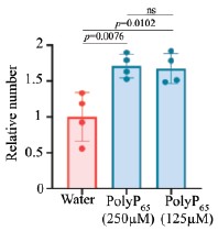
Reviewer #3 (Public review):
Summary:
Sarkar, Bhandari, Jaiswal, and colleagues establish a suite of quantitative and genetic tools to use Drosophila melanogaster as a model metazoan organism to study polyphosphate (polyP) biology. By adapting biochemical approaches for use in D. melanogaster, they identify a window of increased polyP levels during development. Using genetic tools, they find that depleting polyP from the cytoplasm alters the timing of metamorphosis, accelerating eclosion. By adapting subcellular imaging approaches for D. melanogaster, they observe polyP in the nucleolus of several cell types. They further demonstrate that polyP localizes to cytoplasmic puncta in hemocytes, and further that depleting polyP from the cytoplasm of hemocytes impairs hemolymph clotting. Together, these findings establish D. melanogaster as a tractable system for advancing our understanding of polyP in metazoans.
Strengths:
(1) The FLYX system, combining cell type and compartment-specific expression of ScPpx1, provides a powerful tool for the polyP community.
(2) The finding that cytoplasmic polyP levels change during development and affect the timing of metamorphosis is an exciting first step in understanding the role of polyP in metazoan development, and possible polyP-related diseases.
(3) Given the significant existing body of work implicating polyP in the human blood clotting cascade, this study provides compelling evidence that polyP has an ancient role in clotting in metazoans.
We sincerely thank the reviewer for their generous and insightful comments. Their recognition of both the technical strengths of the FLYX system and the broader biological implications reinforces our confidence that this work will serve as a useful foundation for the community.
Limitations:
(1) While the authors demonstrate that HA-ScPpx1 protein localizes to the target organelles in the various FLYX constructs, the capacity of these constructs to deplete polyP from the different cellular compartments is not shown. This is an important control to both demonstrate that the GTS-PPBD labeling protocol works, and also to establish the efficacy of compartment-specific depletion. While not necessary to do this for all the constructs, it would be helpful to do this for the cyto-FLYX and nuc-FLYX.
We confirmed polyP depletion in Cyto-FLYX using the malachite green assay (Fig. 3D, p.10, l.212–214). The efficacy of ScPpX1 has also been earlier demonstrated in mammalian mitochondria (6). Our preliminary data from Mito-ScPpX1 expressed ubiquitously with Tubulin-Gal4 showed a reduction in polyP levels when estimated from whole flies (See Author response image 2 below, ongoing investigation). In an independent study focusing on mitochondrial polyP depletion, we are characterizing these lines in detail and plan to check the amount of polyP contributed to the cellular pool by mitochondria using subcellular fractionation. Direct phenotypic and polyP depletion analyses of Nuc-FLYX and ER-FLYX are also being carried out, but are in preliminary stages. That there is a difference in levels of polyP in various tissues and that we get a very little subscellular fraction for polyP analysis have been a few challenging issues. This analysis requires detailed, independent, and careful analysis, and thus, we refrain from adding this data to the current manuscript.
Author response image 2.
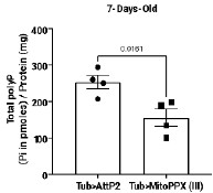
Regarding the specificity, Saito et.al. reported that PPBD binds to polyP in vitro, as well as in yeast and mammalian cells with a high affinity of ~45µM for longer polyP chains (35 mer and above) (3). They also show that the affinity of PPBD with RNA and DNA is very low. Further, PPBD could reveal differences in polyP labeling with yeasts grown in different physiological conditions that can alter polyP levels. Now in the manuscript, we included following data to show specificity of PPBD:
To address this concern we have done two sets of experiments:
We generated a PPBD mutant (GST-PPBD<sup>Mut</sup>). Using Microscale Thermophoresis, we establish that GST-PPBD binds to polyP<sub>100</sub>-2X-FITC, whereas, GST-PPBD<sup>Mut</sup> and GST do not bind polyP<sub>100</sub>-2X-FITC at all. We found that unlike the punctate staining pattern of GST-PPBD (wild-type), GST-PPBD<sup>Mut</sup> does not stain hemocytes. This data has been added to the revised manuscript (Fig. 2B-D, p.8, l.151–165).
A study in C.elegans by Quarles et.al has performed a similar experiment suggested by the reviewer. In that study, treating permeabilized tissues with polyphosphatase prior to PPBD staining resulted in decrease of PPBD-GFP signal from the tissues (2). We also performed the same experiment where we subjected hemocytes to GST-PPBD staining with prior incubation of fixed and permeabilised hemocytes with ScPpX1 and heat inactivated ScPpX1 protein. We find that both intensity of staining and number of punctae are higher in hemocytes that were left untreated and the one where heat inactivated ScPpX1 was added. The hemocytes pre-treated with ScPpX1 showed reduced staining intensity and number of punctae. This data has been added to the revised manuscript (Fig. 2E-G, p.8, l.166-172).
(2) The cell biological data in this study clearly indicates that polyP is enriched in the nucleolus in multiple cell types, consistent with recent findings from other labs, and also that polyP affects gene expression during development. Given that the authors also generate the Nuc-FLYX construct to deplete polyP from the nucleus, it is surprising that they test how depleting cytoplasmic but not nuclear polyP affects development. However, providing these tools is a service to the community, and testing the phenotypic consequences of all the FLYX constructs may arguably be beyond the scope of this first study.
We agree this is an important avenue. In this first study, we focused on establishing the toolkit and reporting phenotypes with Cyto-FLYX. We are systematically assaying phenotypes from all FLYX constructs, including Nuc-FLYX, in ongoing studies
Recommendations for the authors:
Reviewing Editor Comment:
The reviewers appreciated the general quality of the rigour and work presented in this manuscript. We also had a few recommendations for the authors. These are listed here and the details related to them can be found in the individual reviews below.
(1) We suggest including an appropriate control to show that PPBD binds polyP specifically.
We have updated the response section as follows:
(a) Highlighted previous literature that showed the specificity of PPBD.
(b) We show that the punctate staining observed by PPBD is not demonstrated by the mutant PPBD (PPBD<sup>Mut</sup>) in which amino acids that are responsible for polyP binding are mutated.
(c) We show that PPBD<sup>Mut</sup> does not bind to polyP using Microscale Thermophoresis.
(d) We show that treatment of fixed and permeabilised hemocytes with ScPpX1 reduces the PPBD staining intensity and number of punctae, as compared to tissues left untreated or treated with heat-inactivated ScPpX1.
We have included these in our updated revised manuscript (Fig. 2B-G, p.8, l.151–157)
(2) The high concentration of PolyP in the clotting assay might be impeding clotting. The authors may want to consider lowering this in their assays.
We have addressed this concern in our revised manuscript. We have performed the clotting assays with lower polyP concentrations (concentrations previously used in clotting experiments with human blood and polyP). Data is included in Fig. S5F–I, p.12, l.241–243.
(3) The RNAseq study: can the authors please describe this better and possibly mine it for the regulation of genes that affect eclosion?
In our revised manuscript, we have included a broader discussion about the RNAseq analysis done in the article in both the ‘results’ and the ‘discussion’ sections, where we have rewritten the narrative from the perspective of accelerated eclosion. (p.15 l.310-335, p. 20, l.431-446).
(4) Have the authors considered the possibility that the gut microbiota might be contributing to some of their measurements and assays? It would be good to address this upfront - either experimentally, in the discussion, or (ideally) both.
This is an exciting possibility. Several observations argue that fly tissues synthesize polyP: (i) polyP levels remain very low during feeding stages but build up in wandering third instar larvae after feeding ceases; (ii) PPBD staining is absent from the gut except the crop (Fig. S3O–P); (iii) in C. elegans, intestinal polyP was unaffected when worms were fed polyP-deficient bacteria (2); (iv) depletion of polyP from plasmatocytes alone impairs hemolymph clotting, which would not be expected if gut-derived polyP were the major source and may have contributed to polyP in hemolymph. Nevertheless, microbiota-derived polyP may contribute, and we plan systematic testing in axenic flies in future work.
Reviewer #1 (Recommendations for the authors):
(1) While the authors have shown that the depletion tool results in a general reduction of polyP levels in Figure 3D, it would have been nice to show this via IHC. Particularly since the depletion depends on the strength of the Gal4, it is possible that the phenotypes are being under-estimated because the depletions are weak.
We agree that different Gal4 lines have different strengths and will therefore affect polyP levels and the strength of the phenotype differently.
We performed PPBD staining on hemocytes expressing ScPPX; however, we observed very intense, uniform staining throughout the cells, which was unexpected. It seems like PPBD is recognizing overexpressed ScPpX1. Indeed, in an unpublished study by Manisha Mallick (Bhandari lab), it was found that His-ScPpX1 specifically interacts with GST-PPBD in a protein interaction assay (See Author response image 3). Due to these issues, we refrained from IHC/PPBD-based validation.
Author response image 3.
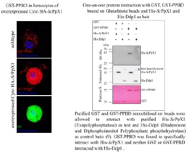
(2) The subcellular tools for depletion are neat! I wonder why the authors didn't test them. For example in the salivary gland for nuclear depletion?
We have addressed this question in the reviewer responses. We are systematically assaying phenotypes from all FLYX constructs, including Mito-FLYX, and Nuc-FLYX, in ongoing independent investigations. As discussed in #1, a possible interaction of ScPpX and PPBD is making this test a bit more challenging, and hence, they each require a detailed investigation.
(a) Does the absence of clotting defects using Lz-gal4 suggest that PolyP is more crucial in the plasmatocytoes and for the initial clotting process? And that it is dispensible/less important in the crystal cells and for the later clotting process. Or is it that the crystal cells just don't have as much polyP? The image (2E-H) certainly looks like it.
In hemolymph, the primary clot formation is a result of the clotting factors secreted from the fat bodies and the plasmatocytes. The crystal cells are responsible for the release of factors aiding in successfully hardening the soft clot initially formed. Reports suggest that clotting and melanization of the clot are independent of each other (7). Since Crystal cells do not contribute to clot fibre formation, the absence of clotting defects using LzGAL4-CytoFLYX is not surprising. Alternatively, PolyP may be secreted from all hemocytes and contribute to clotting; however, the crystal cells make up only 5% hemocytes, and hence polyP depletion in those cells may have a negligible effect on blood clotting.
Crystal cells do show PPBD staining. Whether polyP is significantly lower in levels in the crystal cells as compared to the plasmatocytes needs more systematic investigation. Image (2E-H) is a representative image of the presence of polyP in crystal cells and can not be considered to compare polyP levels in the crystal cells vs Plasmatocytes.
(b) The RNAseq analyses and data could be better presented. If the data are indeed variable and the differentially expressed genes of low confidence, I might remove that data entirely. I don't think it'll take away from the rest of the work.
We understand this concern and, therefore, in the revised manuscript, we have included a broader discussion about the RNAseq analysis done in the article in both the ‘results’ and the ‘discussion’ sections, where we have rewritten the narrative from the perspective of accelerated eclosion. (p.15 l.310-335, p. 20, l.431-446). We have also stated the limitations of such studies.
(c) I would re-phrase the first sentence of the results section.
We have re-phrased it in the revised manuscript.
Reviewer #2 (Recommendations for the authors):
(1) The authors created several different versions of the FLYX system that would be targeted to different subcellular compartments. They mostly report on the effects of cytosolic targeting, but some of the constructs targeted the polyphosphatase to mitochondria or the nucleus.
They report that the targeting worked, but I didn't see any results on the effects of those constructs on fly viability, development, etc.
There is a growing literature of investigators targeting polyphosphatase to mitochondria and showing how depleting mitochondrial polyP alters mitochondrial function. What was the effect of the Nuc-FLYX and Mito-FLYX constructs on the flies?
Also, the authors should probably cite the papers of others on the effects of depleting mitochondrial polyP in other eukaryotic cells in the context of discussing their findings in flies.
We have addressed this question in the reviewer responses. We did not see any obvious developmental or viability defects with any of the FLYX lines, and only after careful investigation did we come across the clotting defects in the CytoFLYX. We are currently systematically assaying phenotypes from all FLYX constructs, including Mito-FLYX and Nuc-FLYX, in independent ongoing investigations.
We have discussed the heterologous expression of mitochondrial polyphosphatase in mammalian cells to justify the need for developing Mito-FLYX (p. 10, l. 197-200). In the discussion section, we also discuss the presence and roles of polyP in the nucleus and how Nuc-FLYX can help study such phenomena (p. 19, l. 399-407).
(2) The authors should number the pages of their manuscript to make it easier for reviewers to refer to specific pages.
We have numbered our lines and pages in the revised manuscript.
(3) Abstract: the abbreviation, "polyP", is not defined in the abstract. The first word in the abstract is "polyphosphate", so it should be defined there.
We have corrected it in the revised version.
(4) The authors repeatedly use the phrase, "orange hot", to describe one of the colors in their micrographs, but I don't know how this differs from "orange".
‘OrangeHot’ is the name of the LUT used in the ImageJ analysis and hence referred to as the colour
(5) First page of the Introduction: the phrase, "feeding polyP to αβ expression Alzheimer's model of Caenorhabditis elegans" is awkward (it literally means feeding polyP to the model instead of the worms).
We have revised it. (p.3, l.55-57).
(6) Page 2 of the Introduction: The authors should cite this paper when they state that NUDT3 is a polyphosphatase: https://pubmed.ncbi.nlm.nih.gov/34788624/
We have cited the paper in the revised version of the manuscript. (p.4, l. 68-70)
(7) Page 2 of Results: The authors report the polyP content in the third instar larva (misspelled as "larval") to five significant digits ("419.30"). Their data do not support more than three significant digits, though.
We have corrected it in the revised manuscript.
(8) Page 3 of Results (paragraph 1): When discussing the polyP levels in various larval stages, the authors are extracting total polyP from the larvae. It seems that at least some of the polyP may come from gut microbes. This should probably be mentioned.
This is an interesting possibility. Several observations argue that polyP is synthesized by fly tissues: (i) polyP levels remain very low during feeding stages but build up in wandering third instar larvae after feeding ceases; (ii) PPBD staining is absent from the gut except the crop (Fig. S3O–P); (ii) In C. elegans, intestinal polyP was unaffected when worms were fed polyP-deficient bacteria (2); (iv) depletion of polyP from plasmatocytes alone impairs hemolymph clotting, which would not be expected if gut-derived polyP were the major source and may have contributed to polyP in hemolymph. We mention this limitation in the revised manuscript (p.19-20, l. 425-433).
(9) Page 3 of Results (paragraph 2): stating that the 4% paraformaldehyde works "best" is imprecise. What do the authors mean by "best"?
We have addressed this comment in the revised manuscript and corrected it as 4% paraformaldehyde being better among the three methods we used to fix tissues, which also included methanol and Bouin’s fixative (p.8, l. 152-154).
(10) Page 4 of Results (paragraph 2, last line of the page): The scientific literature is vast, so one can never be sure that one knows of all the papers out there, even on a topic as relatively limited as polyP. Therefore, I would recommend qualifying the statement "...this is the first comprehensive tissue staining report...". It would be more accurate (and safer) to say something like, "to our knowledge, this is the first..." There is a similar statement with the word "first" on the next page regarding the FLYX library.
We have addressed this concern and corrected it accordingly in the revised version of the manuscript (p.9, l. 192-193)
Reviewer #3 (Recommendations for the authors):
(1) The authors should include in their discussion a comparison of cell biological observations using the polyP binding domain of E. coli Ppx (GST-PPBD) to fluorescently label polyP in cells and tissues with recent work using a similar approach in C. elegans (Quarles et al., PMID:39413779).
In the revised manuscript, we have cited the work of Quarles et al. and have added a comparison of observations (p.19,l.408-410). In the discussion, we have also focused on multiple other studies about how polyP presence in different subcellular compartments, like the nucleus, can be assayed and studied with the tools developed in this study.
(2) The gene expression studies of time-matched Cyto-FLYX vs WT larvae is very intriguing. Given the authors' findings that non-feeding third instar Cyto-FLYX larvae are developmentally ahead of WT larvae, can the observed trends be explained by known changes in gene expression that occur during eclosion? This is mentioned in the results section in the context of genes linked to neurons, but a broader discussion of which pathway changes observed can be explained by the developmental stage difference between the WT and FLYX larvae would be helpful in the discussion.
We have included a broader discussion about the RNAseq analysis done in the article in both the ‘results’ and the ‘discussion’ sections, where we have rewritten the narrative from the perspective of accelerated eclosion. (p.15 l.310-335, p. 20, l.431-446). We have also stated the limitations of such studies.
(3) The sentence describing NUDT3 is not referenced.
We have addressed this comment and have cited the paper of NUDT3 in the revised version of the manuscript.(p.4, l. 68-70)
(4) In the first sentence of the results section, the meaning/validity of the statement "The polyP levels have decreased as evolution progressed" is not clear. It might be more straightforward to give an estimate of the total pmoles polyP/mg protein difference between bacteria/yeast and metazoans.
In the revised manuscript, we have given an estimate of the polyP content across various species across evolution to uphold the statement that polyP levels have decreased as evolution progressed (p. 5, l. 87-91).
(5) The description of the malachite green assay in the results section describes it as "calorimetric" but this should read "colorimetric?"
We have corrected it in the revised manuscript.
References
(1) Chicco D, Agapito G. Nine quick tips for pathway enrichment analysis. PLoS Comput Biol. 2022 Aug 11;18(8):e1010348.
(2) Quarles E, Petreanu L, Narain A, Jain A, Rai A, Wang J, et al. Cryosectioning and immunofluorescence of C. elegans reveals endogenous polyphosphate in intestinal endo-lysosomal organelles. Cell Rep Methods. 2024 Oct 8;100879.
(3) Saito K, Ohtomo R, Kuga-Uetake Y, Aono T, Saito M. Direct labeling of polyphosphate at the ultrastructural level in Saccharomyces cerevisiae by using the affinity of the polyphosphate binding domain of Escherichia coli exopolyphosphatase. Appl Environ Microbiol. 2005 Oct;71(10):5692–701.
(4) Smith SA, Mutch NJ, Baskar D, Rohloff P, Docampo R, Morrissey JH. Polyphosphate modulates blood coagulation and fibrinolysis. Proc Natl Acad Sci USA. 2006 Jan 24;103(4):903–8.
(5) Smith SA, Choi SH, Davis-Harrison R, Huyck J, Boettcher J, Rienstra CM, et al. Polyphosphate exerts differential effects on blood clotting, depending on polymer size. Blood. 2010 Nov 18;116(20):4353–9.
(6) Abramov AY, Fraley C, Diao CT, Winkfein R, Colicos MA, Duchen MR, et al. Targeted polyphosphatase expression alters mitochondrial metabolism and inhibits calcium-dependent cell death. Proc Natl Acad Sci USA. 2007 Nov 13;104(46):18091–6.
(7) Schmid MR, Dziedziech A, Arefin B, Kienzle T, Wang Z, Akhter M, et al. Insect hemolymph coagulation: Kinetics of classically and non-classically secreted clotting factors. Insect Biochem Mol Biol. 2019 Jun;109:63–71.
(8) Jian Guan, Rebecca Lee Hurto, Akash Rai, Christopher A. Azaldegui, Luis A. Ortiz-Rodríguez, Julie S. Biteen, Lydia Freddolino, Ursula Jakob. HP-Bodies – Ancestral Condensates that Regulate RNA Turnover and Protein Translation in Bacteria. bioRxiv 2025.02.06.636932; doi: https://doi.org/10.1101/2025.02.06.636932.
(9) Lonetti A, Szijgyarto Z, Bosch D, Loss O, Azevedo C, Saiardi A. Identification of an evolutionarily conserved family of inorganic polyphosphate endopolyphosphatases. J Biol Chem. 2011 Sep 16;286(37):31966–74.
Author response:
The following is the authors’ response to the original reviews.
Reviewer #1
Chen et al. engineered and characterized a suite of next-generation GECIs for the Drosophila NMJ that allow for the visualization of calcium dynamics within the presynaptic compartment, at presynaptic active zones, and in the postsynaptic compartment. These GECIs include ratiometric presynaptic Scar8m (targeted to synaptic vesicles), ratiometric active zone localized Bar8f (targeted to the scaffold molecule BRP), and postsynaptic SynapGCaMP8m. The authors demonstrate that these new indicators are a large improvement on the widely used GCaMP6 and GCaMP7 series GECIs, with increased speed and sensitivity. They show that presynaptic Scar8m accurately captures presynaptic calcium dynamics with superior sensitivity to the GCaMP6 and GCaMP7 series and with similar kinetics to chemical dyes. The active-zone targeted Bar8f sensor was assessed for the ability to detect release-site-specific nanodomain changes, but the authors concluded that this sensor is still too slow to accurately do so. Lastly, the use of postsynaptic SynapGCaMP8m was shown to enable the detection of quantal events with similar resolution to electrophysiological recordings. Finally, the authors developed a Python-based analysis software, CaFire, that enables automated quantification of evoked and spontaneous calcium signals. These tools will greatly expand our ability to detect activity at individual synapses without the need for chemical dyes or electrophysiology.
We thank this Reviewer for the overall positive assessment of our manuscript and for the incisive comments.
(1) The role of Excel in the pipeline could be more clearly explained. Lines 182-187 could be better worded to indicate that CaFire provides analysis downstream of intensity detection in ImageJ. Moreover, the data type of the exported data, such as .csv or .xlsx, should be indicated instead of 'export to graphical program such as Microsoft Excel'.
We thank the Reviewer for these comments, many of which were shared by the other reviewers. In response, we have now 1) more clearly explained the role of Excel in the CaFire pipeline (lines 677-681), 2) revised the wording in lines 676-679 to indicate that CaFire provides analysis downsteam of intensity detection in ImageJ, and 3) Clarified the exported data type to Excel (lines 677-681). These efforts have improved the clarity and readability of the CaFire analysis pipeline.
(2) In Figure 2A, the 'Excel' step should either be deleted or included as 'data validation' as ImageJ exports don't require MS Excel or any specific software to be analysed. (Also, the graphic used to depict Excel software in Figure 2A is confusing.)
We thank the reviewer for this helpful suggestion. In the Fig. 2A, we have changed the Excel portion and clarified the processing steps in the revised methods. Specifically, we now indicate that ROIs are first selected in Fiji/ImageJ and analyzed to obtain time-series data containing both the time information and the corresponding imaging mean intensity values. These data are then exported to a spreadsheet file (e.g., Excel), which is used to organize the output before being imported into CaFire for subsequent analysis. These changes can be found in the Fig. 2A and methods (lines 676-681).
(3) Figure 2B should include the 'Partition Specification' window (as shown on the GitHub) as well as the threshold selection to give the readers a better understanding of how the tool works.
We absolutely agree with this comment, and have made the suggested changes to the Fig. 2B. In particular, we have replaced the software interface panels and now include windows illustrating the Load File, Peak Detection, and Partition functions. These updated screenshots provide a clearer view of how CaFire is used to load the data, detect events, and perform partition specification for subsequent analysis. We agree these changes will give the readers a better understanding of how the tool works, and we thank the reviewer for this comment.
(4) The presentation of data is well organized throughout the paper. However, in Figure 6C, it is unclear how the heatmaps represent the spatiotemporal fluorescence dynamics of each indicator. Does the signal correspond to a line drawn across the ROI shown in Figure 6B? If so, this should be indicated.
We apologize that the heatmaps were unclear in Fig panel 6C (Fig. 7C in the Current revision). Each heatmap is derived from a one-pixel-wide vertical line within a miniature-event ROI. These heatmaps correspond to the fluorescence change in the indicated SynapGCaMP variant of individual quantal events and their traces shown in Fig. 7C, with a representative image of the baseline and peak fluorescence shown in Fig. 7B. Specifically, we have added the following to the revised Fig. 7C legend:
The corresponding heatmaps below were generated from a single vertical line extracted from a representative miniature-event ROI, and visualize the spatiotemporal fluorescence dynamics (ΔF/F) along that line over time.
(5) In Figure 6D, the addition of non-matched electrophysiology recordings is confusing. Maybe add "at different time points" to the end of the 6D legend, or consider removing the electrophysiology trace from Figure 6D and referring the reader to the traces in Figure 7A for comparison (considering the same point is made more rigorously in Figure 7).
This is a good point, one shared with another reviewer. We apologize this was not clear, and have now revised this part of the figure to remove the electrophysiological traces in what is now Fig. 7 while keeping the paired ones still in what is now Fig. 8A as suggested by the reviewer. We agree this helps to clarify the quantal calcium transients.
(6) In GitHub, an example ImageJ Script for analyzing the images and creating the inputs for CaFire would be helpful to ensure formatting compatibility, especially given potential variability when exporting intensity information for two channels. In the Usage Guide, more information would be helpful, such as how to select ∆R/R, ideally with screenshots of the application being used to analyze example data for both single-channel and two-channel images.
We agree that additional details added to the GitHub would be helpful for users of CaFire. In response, we have now added the following improvements to the GitHub site:
- ImageJ operation screenshots
Step-by-step illustrations of ROI drawing and Multi Measure extraction.
- Example Excel file with time and intensity values
Demonstrates the required data format for CaFire import, including proper headers.
- CaFire loading screenshots for single-channel and dual-channel imaging
Shows how to import GCaMP into Channel 1 and mScarlet into Channel 2.
- Peak Detection and Partition setting screenshots
Visual examples of automatic peak detection, manual correction, and trace partitioning.
- Instructions for ROI Extraction and CaFire Analysis
A written guide describing the full workflow from ROI selection to CaFire data export.
These changes have improved the usability and accessibility of CaFire, and we thank the reviewer for these points.
Reviewer #2
Calcium ions play a key role in synaptic transmission and plasticity. To improve calcium measurements at synaptic terminals, previous studies have targeted genetically encoded calcium indicators (GECIs) to pre- and postsynaptic locations. Here, Chen et al. improve these constructs by incorporating the latest GCaMP8 sensors and a stable red fluorescent protein to enable ratiometric measurements. In addition, they develop a new analysis platform, 'CaFire', to facilitate automated quantification. Using these tools, the authors demonstrate favorable properties of their sensors relative to earlier constructs. Impressively, by positioning postsynaptic GCaMP8m near glutamate receptors, they show that their sensors can report miniature synaptic events with speed and sensitivity approaching that of intracellular electrophysiological recordings. These new sensors and the analysis platform provide a valuable tool for resolving synaptic events using all-optical methods.
We thank the Reviewer for their overall positive evaluation and comments.
Major comments:
(1) While the authors rigorously compared the response amplitude, rise, and decay kinetics of several sensors, key parameters like brightness and photobleaching rates are not reported. I feel that including this information is important as synaptically tethered sensors, compared to freely diffusible cytosolic indicators, can be especially prone to photobleaching, particularly under the high-intensity illumination and high-magnification conditions required for synaptic imaging. Quantifying baseline brightness and photobleaching rates would add valuable information for researchers intending to adopt these tools, especially in the context of prolonged or high-speed imaging experiments.
This is a good point made by the reviewer, and one we agree will be useful for researchers to be aware. First, it is important to note that the photobleaching and brightness of the sensors will vary depending on the nature of the user’s imaging equipment, which can vary significantly between widefield microscopes (with various LED or halogen light sources for illumination), laser scanning systems (e.g., line scans with confocal systems), or area scanning systems using resonant scanners (as we use in our current study). Under the same imaging settings, GCaMP8f and 8m exhibit comparable baseline fluorescence, whereas GCaMP6f and 6s are noticeably dimmer; because our aim is to assess each reagent’s potential under optimal conditions, we routinely adjust excitation/camera parameters before acquisition to place baseline fluorescence in an appropriate dynamic range. As an important addition to this study, motivated by the reviewer’s comments above, we now directly compare neuronal cytosolic GCaMP8m expression with our Scar8m sensor, showing higher sensitivity with Scar8m (now shown in the new Fig. 3F-H).
Regarding photobleaching, GCaMP signals are generally stable, while mScarlet is more prone to bleaching: in presynaptic area scanned confocal recordings, the mScarlet channel drops by ~15% over 15 secs, whereas GCaMP6s/8f/8m show no obvious bleaching over the same window (lines 549-553). In contrast, presynaptic widefield imaging using an LED system (CCD), GCaMP8f shows ~8% loss over 15 secs (lines 610-611). Similarly, for postsynaptic SynapGCaMP6f/8f/8m, confocal resonant area scans show no obvious bleaching over 60 secs, while widefield shows ~2–5% bleaching over 60 secs (lines 634-638). Finally, in active-zone/BRP calcium imaging (confocal), mScarlet again bleaches by ~15% over 15 s, while GCaMP8f/8m show no obvious bleaching. The mScarlet-channel bleaching can be corrected in Huygens SVI (Bleaching correction or via the Deconvolution Wizard), whereas we avoid applying bleaching correction to the green GCaMP channel when no clear decay is present to prevent introducing artifacts. This information is now added to the methods (lines 548-553).
(2) In several places, the authors compare the performance of their sensors with synthetic calcium dyes, but these comparisons are based on literature values rather than on side-by-side measurements in the same preparation. Given differences in imaging conditions across studies (e.g., illumination, camera sensitivity, and noise), parameters like indicator brightness, SNR, and photobleaching are difficult to compare meaningfully. Additionally, the limited frame rate used in the present study may preclude accurate assessment of rise times relative to fast chemical dyes. These issues weaken the claim made in the abstract that "...a ratiometric presynaptic GCaMP8m sensor accurately captures .. Ca²⁺ changes with superior sensitivity and similar kinetics compared to chemical dyes." The authors should clearly acknowledge these limitations and soften their conclusions. A direct comparison in the same system, if feasible, would greatly strengthen the manuscript.
We absolutely agree with these points made the reviewer, and have made a concerted effort to address them through the following:
We have now directly compared presynaptic calcium responses on the same imaging system using the chemical dye Oregon Green Bapta-1 (OGB-1), one of the primary synthetic calcium indicators used in our field. These experiments reveal that Scar8f exhibits markedly faster kinetics and an improved signal-to-noise ratio compared to OGB-1, with higher peak fluorescence responses (Scar8f: 0.32, OGB-1: 0.23). The rise time constants of the two indicators are comparable (both ~3 msecs), whereas the decay of Scar8f is faster than that of OGB-1 (Scar8f: ~40, OGB-1: ~60), indicating more rapid signal recovery. These results now directly demonstrate the superiority of the new GCaMP8 sensors we have engineered over conventional synthetic dyes, and are now presented in the new Fig. 3A-E of the manuscript.
We agree with the reviewer that, in the original submission, the relatively slow resonant area scans (~115 fps) limited the temporal resolution of our rise time measurements. To address this, we have re-measured the rise time using higher frame-rate line scans (kHz). For Scar8f, the rise time constant was 6.736 msec at ~115 fps resonant area scanned, but shortened to 2.893 msec when imaged at ~303 fps, indicating that the original protocol underestimated the true kinetics. In addition, for Bar8m, area scans at ~118 fps yielded a rise time constant of 9.019 msec, whereas line scans at ~1085 fps reduced the rise time constant to 3.230 msec. These new measurements are now incorporated into the manuscript ( Figs. 3,4, and 6) to more accurately reflect the fast kinetics of these indicators.
(3) The authors state that their indicators can now achieve measurements previously attainable with chemical dyes and electrophysiology. I encourage the authors to also consider how their tools might enable new measurements beyond what these traditional techniques allow. For example, while electrophysiology can detect summed mEPSPs across synapses, imaging could go a step further by spatially resolving the synaptic origin of individual mEPSP events. One could, for instance, image MN-Ib and MN-Is simultaneously without silencing either input, and detect mEPSP events specific to each synapse. This would enable synapse-specific mapping of quantal events - something electrophysiology alone cannot provide. Demonstrating even a proof-of-principle along these lines could highlight the unique advantages of the new tools by showing that they not only match previous methods but also enable new types of measurements.
These are excellent points raised by the reviewer. In response, we have done the following:
We have now included a supplemental video as “proof-of-principle” data showing simultaneous imaging of SynapGCaMP8m quantal events at both MN-Is and -Ib, demonstrating that synapse-specific spatial mapping of quantal events can be obtained with this tool (see new Supplemental Video 1).
We have also included an additional discussion of the potential and limitations of these tools for new measurements beyond conventional approaches. This discussion is now presented in lines 419-421 in the manuscript.
(4) For ratiometric measurements, it is important to estimate and subtract background signals in each channel. Without this correction, the computed ratio may be skewed, as background adds an offset to both channels and can distort the ratio. However, it is not clear from the Methods section whether, or how, background fluorescence was measured and subtracted.
This is a good point, and we agree more clarification about how ratiometric measurements were made is needed. In response, we have now added the following to the Methods section (lines 548-568):
Time-lapse videos were stabilized and bleach-corrected prior to analysis, which visibly reduced frame-toframe motion and intensity drift. In the presynaptic and active-zone mScarlet channel, a bleaching factor of ~1.15 was observed during the 15 sec recording. This bleaching can be corrected using the “Bleaching correction” tool in Huygens SVI. For presynaptic and active-zone GCaMP signals, there was minimal bleaching over these short imaging periods. Therefore, the bleaching correction step for GCaMP was skipped. Both GCaMP and mScarlet channels were processed using the default settings in the Huygens SVI “Deconvolution Wizard” (with the exception of the bleaching correction option). Deconvolution was performed using the CMLE algorithm with the Huygens default stopping criterion and a maximum of 30 iterations, such that the algorithm either converged earlier or, if convergence was not reached, was terminated at this 30iteration limit; no other iteration settings were used across the GCaMP series. ROIs were drawn on the processed images using Fiji ImageJ software, and mean fluorescence time courses were extracted for the GCaMP and mScarlet channels, yielding F<sub>GCaMP</sub>(t) and F<sub>mScarlet</sub>(t). F(t)s were imported into CaFire with GCaMP assigned to Channel #1 (signal; required) and mScarlet to Channel #2 (baseline/reference; optional). If desired, the mScarlet signal could be smoothed in CaFire using a user-specified moving-average window to reduce high-frequency noise. In CaFire’s ΔR/R mode, the per-frame ratio was computed as R(t)=F<sub>GCaMP</sub>(t) and F<sub>mScarlet</sub>(t); a baseline ratio R0 was estimated from the pre-stimulus period, and the final response was reported as ΔR/R(t)=[R(t)−R0]/R0, which normalizes GCaMP signals to the co-expressed mScarlet reference and thereby reduces variability arising from differences in sensor expression level or illumination across AZs.
(5) At line 212, the authors claim "... GCaMP8m showing 345.7% higher SNR over GCaMP6s....(Fig. 3D and E) ", yet the cited figure panels do not present any SNR quantification. Figures 3D and E only show response amplitudes and kinetics, which are distinct from SNR. The methods section also does not describe details for how SNR was defined or computed.
This is another good point. We define SNR operationally as the fractional fluorescence change (ΔF/F). Traces were processed with CaFire, which estimates a per-frame baseline F<sub>0</sub>(t) with a user-configurable sliding window and percentile. In the Load File panel, users can specify both the length of the moving baseline window and the desired percentile; the default settings are a 50-point window and the 30th percentile, representing a 101-point window centered on each time point (previous 50 to next 50 samples) and took the lower 30% of values within that window to estimate F<sub>0</sub>(t). The signal was then computed as ΔF/F=[F(t)−F0(t)]/F0(t). This ΔF/F value is what we report as SNR throughout the manuscript and is now discussed explicitly in the revised methods (lines 686-693).
(6) Lines 285-287 "As expected, summed ΔF values scaled strongly and positively with AZ size (Fig. 5F), reflecting a greater number of Cav2 channels at larger AZs". I am not sure about this conclusion. A positive correlation between summed ΔF values and AZ size could simply reflect more GCaMP molecules in larger AZs, which would give rise to larger total fluorescence change even at a given level of calcium increase.
The reviewer makes a good point, one that we agree should be clarified. The reviewer is indeed correct that larger active zones should have more abundant BRP protein, which in turn will lead to a higher abundance of the Bar8f sensor, which should lead to a higher GCaMP response simply by having more of this sensor. However, the inclusion of the ratiometric mScarlet protein should normalize the response accurately, correcting for this confound, in which the higher abundance of GCaMP should be offset (normalized) by the equally (stoichiometric) higher abundance of mScarlet. Therefore, when the ∆R/R is calculated, the differences in GCaMP abundance at each AZ should be corrected for the ratiometric analysis. We now use an improved BRP::mScarlet3::GCaMP8m (Bar8m) and compute ΔR/R with R(t)=F<sub>GCaMP8m</sub>/F<sub>mScarlet3</sub>. ROIs were drawn over individual AZs (Fig. 6B). CaFire estimated R0 with a sliding 101-point window using the lowest 10% of values, and responses were reported as ΔR/R=[R−R0]/R0. Area-scan examples (118 fps) show robust ΔR/R transients (peaks ≈1.90 and 3.28; tau rise ≈9.0–9.3 ms; Fig. 6C, middle).
We have now made these points more clearly in the manuscript (lines 700-704) and moved the Bar8f intensity vs active zone size data to Table S1. Together, these revisions improve the indicator-abundance confound (via mScarlet normalization).
(6) Lines 313-314: "SynapGCaMP quantal signals appeared to qualitatively reflect the same events measured with electrophysiological recordings (Fig. 6D)." This statement is quite confusing. In Figure 6D, the corresponding calcium and ephys traces look completely different and appear to reflect distinct sets of events. It was only after reading Figure 7 that I realized the traces shown in Figure 6D might not have been recorded simultaneously. The authors should clarify this point.
Yes, we absolutely agree with this point, one shared by Reviewer 1. In response, we have removed the electrophysiological traces in Fig. 6 to clarify that just the calcium responses are shown, and save the direct comparison for the Fig. 7 data (now revised Fig. 8).
(8) Lines 310-313: "SynapGCaMP8m .... striking an optimal balance between speed and sensitivity", and Lines 314-316: "We conclude that SynapGCaMP8m is an optimal indicator to measure quantal transmission events at the synapse." Statements like these are subjective. In the authors' own comparison, GCaMP8m is significantly slower than GCaMP8f (at least in terms of decay time), despite having a moderately higher response amplitude. It is therefore unclear why GCaMP8m is considered 'optimal'. The authors should clarify this point or explain their rationale for prioritizing response amplitude over speed in the context of their application.
This is another good point that we agree with, as the “optimal” sensor will of course depend on the user’s objectives. Hence, we used the term “an optimal sensor” to indicate it is what we believed to be the best one for our own uses. However, this point should be clarified and better discussed. In response, we have revised the relevant sections of the manuscript to better define why we chose the 8m sensors to strike an optimal balance of speed and sensitivity for our uses, and go on to discuss situations in which other sensor variants might be better suited. These are now presented in lines 223-236 in the revised manuscript, and we thank the reviewer for making these comments, which have improved our study.
Minor comments
(1) Please include the following information in the Methods section:
(a) For Figures 3 and 4, specify how action potentials were evoked. What type of electrodes were used, where were they placed, and what amount of current or voltage was applied?
We apologize for neglecting to include this information in the original submission. We have now added this information to the revised Methods section (lines 537-543).
(b) For imaging experiments, provide information on the filter sets used for each imaging channel, and describe how acquisition was alternated or synchronized between the green and red channels in ratiometric measurements. Additionally, please report the typical illumination intensity (in mW/mm²) for each experimental condition.
We thank the reviewer for this helpful comment. We have now added detailed information about the imaging configuration to the Methods (lines 512-528) with the following:
Ca2+ imaging was conducted using a Nikon A1R resonant scanning confocal microscope equipped with a 60x/1.0 NA water-immersion objective (refractive index 1.33). GCaMP signals were acquired using the FITC/GFP channel (488-nm laser excitation; emission collected with a 525/50-nm band-pass filter), and mScarlet/mCherry signals were acquired using the TRITC/mCherry channel (561-nm laser excitation; emission collected with a 595/50-nm band-pass filter). ROIs focused on terminal boutons of MN-Ib or -Is motor neurons. For both channels, the confocal pinhole was set to a fixed diameter of 117.5 µm (approximately three Airy units under these conditions), which increases signal collection while maintaining adequate optical sectioning. Images were acquired as 256 × 64 pixel frames (two 12-bit channels) using bidirectional resonant scanning at a frame rate of ~118 frames/s; the scan zoom in NIS-Elements was adjusted so that this field of view encompassed the entire neuromuscular junction and was kept constant across experiments. In ratiometric recordings, the 488-nm (GCaMP) and 561-nm (mScarlet) channels were acquired in a sequential dual-channel mode using the same bidirectional resonant scan settings: for each time point, a frame was first collected in the green channel and then immediately in the red channel, introducing a small, fixed frame-to-frame temporal offset while preserving matched spatial sampling of the two channels.
Directly measuring the absolute laser power at the specimen plane (and thus reporting illumination intensity in mW/mm²) is technically challenging on this resonant-scanning system, because it would require inserting a power sensor into the beam path and perturbing the optical alignment; consequently, we are unable to provide reliable absolute mW/mm² values. Instead, we now report all relevant acquisition parameters (objective, numerical aperture, refractive index, pinhole size, scan format, frame rate, and fixed laser/detector settings) and note that laser powers were kept constant within each experimental series and chosen to minimize bleaching and phototoxicity while maintaining an adequate signal-to-noise ratio. We have now added the details requested in the revised Methods section (lines 512-535), including information about the filter sets, acquisition settings, and typical illumination intensity.
(2) Please clarify what the thin versus thick traces represent in Figures 3D, 3F, 4C, and 4E. Are the thin traces individual trials from the same experiment, or from different experiments/animals? Does the thick trace represent the mean/median across those trials, a fitted curve, or a representative example?
We apologize this was not more clear in the original submission. Thin traces are individual stimulus-evoked trials (“sweeps”) acquired sequentially from the same muscle/NMJ in a single preparation; the panel is shown as a representative example of recordings collected across animals. The thick colored trace is the trialaveraged waveform (arithmetic mean) of those thin traces after alignment to stimulus onset and baseline subtraction (no additional smoothing beyond what is stated in Methods). The thick black curve over the decay phase is a single-exponential fit used to estimate τ. Specifically, we fit the decay segment by linear regression on the natural-log–transformed baseline-subtracted signal, which is equivalent to fitting y = y<sub>peak</sub>·e<sup>−t/τdecay</sup> over the decay window (revised Fig.4D and Fig.5C legends).
(3) Please clarify what the reported sample size (n) represents. Does it indicate the number of experimental repeats, the number of boutons or PSDs, or the number of animals?
Again, we apologize this was not clear. (n) refers to the number of animals (biological replicates), which is reported in Supplementary Table 1. All imaging was performed at muscle 6, abdominal segment A3. Per preparation, we imaged 1-2 NMJs in total, with each imaging targeting 2–3 terminal boutons at the target NMJ and acquired 2–3 imaging stacks choosing different terminal boutons per NMJ. For the standard stimulation protocol, we delivered 1 Hz stimulation for 1ms and captured 14 stimuli in a 15s time series imaging (lines 730-736).
Reviewer #3
Genetically encoded calcium indicators (GECIs) are essential tools in neurobiology and physiology. Technological constraints in targeting and kinetics of previous versions of GECIs have limited their application at the subcellular level. Chen et al. present a set of novel tools that overcome many of these limitations. Through systematic testing in the Drosophila NMJ, they demonstrate improved targeting of GCaMP variants to synaptic compartments and report enhanced brightness and temporal fidelity using members of the GCaMP8 series. These advancements are likely to facilitate more precise investigation of synaptic physiology.
This is a comprehensive and detailed manuscript that introduces and validates new GECI tools optimized for the study of neurotransmission and neuronal excitability. These tools are likely to be highly impactful across neuroscience subfields. The authors are commended for publicly sharing their imaging software.
This manuscript could be improved by further testing the GECIs across physiologically relevant ranges of activity, including at high frequency and over long imaging sessions. The authors provide a custom software package (CaFire) for Ca2+ imaging analysis; however, to improve clarity and utility for future users, we recommend providing references to existing Ca2+ imaging tools for context and elaborating on some conceptual and methodological aspects, with more guidance for broader usability. These enhancements would strengthen this already strong manuscript.
We thank the Reviewer for their overall positive evaluation and comments.
Major comments:
(1) Evaluation of the performance of new GECI variants using physiologically relevant stimuli and frequency. The authors took initial steps towards this goal, but it would be helpful to determine the performance of the different GECIs at higher electrical stimulation frequencies (at least as high as 20 Hz) and for longer (10 seconds) (Newman et al, 2017). This will help scientists choose the right GECI for studies testing the reliability of synaptic transmission, which generally requires prolonged highfrequency stimulation.
We appreciate this point by the reviewer and agree it would be of interest to evaluate sensor performance with higher frequency stimulation and for a longer duration. In response, we performed a variety of stimulation protocols at high intensities and times, but found the data to be difficult to separate individual responses given the decay kinetics of all calcium sensors. Hence, we elected not to include these in the revised manuscript. However, we have now included an evaluation of the sensors with 20 Hz electrical stimulation for ~1 sec using a direct comparison of Scar8f with OGB-1. These data are now presented in a new Fig. 3D,E and discussed in the manuscript (lines 396-403).
(2) CaFire.
The authors mention, in line 182: 'Current approaches to analyze synaptic Ca2+ imaging data either repurpose software designed to analyze electrophysiological data or use custom software developed by groups for their own specific needs.' References should be provided. CaImAn comes to mind (Giovannucci et al., 2019, eLife), but we think there are other software programs aimed at analyzing Ca2+ imaging data that would permit such analysis.
Thank you for the thoughtful question. At this stage, we’re unable to provide a direct comparison with existing analysis workflows. In surveying prior studies that analyze Drosophila NMJ Ca²⁺ imaging traces, we found that most groups preprocess images in Fiji/ImageJ and then rely on their own custom-made MATLAB or Python scripts for downstream analysis (see Blum et al. 2021; Xing and Wu 2018). Because these pipelines vary widely across labs, a standardized head-to-head evaluation isn’t currently feasible. With CaFire, our goal is to offer a simple, accessible tool that does not require coding experience and minimizes variability introduced by custom scripts. We designed CaFire to lower the barrier to entry, promote reproducibility, and make quantal event analysis more consistent across users. We have added references to the sentence mentioned above.
Regarding existing software that the reviewer mentioned – CaImAn (Giovannucci et al. 2019): We evaluated CaImAn, which is a powerful framework designed for large-scale, multicellular calcium imaging (e.g., motion correction, denoising, and automated cell/ROI extraction). However, it is not optimized for the per-event kinetics central to our project - such as extracting rise and decay times for individual quantal events at single synapses. Achieving this level of granularity would typically require additional custom Python scripting and parameter tuning within CaImAn’s code-centric interface. This runs counter to CaFire’s design goals of a nocode, task-focused workflow that enables users to analyze miniature events quickly and consistently without specialized programming expertise.
Regarding Igor Pro (WaveMetrics), (Müller et al. 2012): Igor Pro is another platform that can be used to analyze calcium imaging signals. However, it is commercial (paid) software and generally requires substantial custom scripting to fit the specific analyses we need. In practice, it does not offer a simple, open-source, point-and-click path to per-event kinetic quantification, which is what CaFire is designed to provide.
The authors should be commended for making their software publicly available, but there are some questions:
How does CaFire compare to existing tools?
As mentioned above, we have not been able to adapt the custom scripts used by various labs for our purposes, including software developed in MatLab (Blum et al. 2021), Python (Xing and Wu 2018), and Igor (Müller et al. 2012). Some in the field do use semi-publically available software, including Nikon Elements (Chen and Huang 2017) and CaImAn (Giovannucci et al. 2019). However, these platforms are not optimized for the per-event kinetics central to our project - such as extracting rise and decay times for individual quantal events at single synapses. We have added more details about CaFire, mainly focusing on the workflow and measurements, highlighting the superiority of CaFire, showing that CaFire provides a no-code, standardized pipeline with automated miniature-event detection and per-event metrics (e.g., amplitude, rise time τ, decay time τ), optional ΔR/R support, and auto-partition feature. Collectively, these features make CaFire simpler to operate without programming expertise, more transparent and reproducible across users, and better aligned with the event-level kinetics required for this project.
Very few details about the Huygens deconvolution algorithms and input settings were provided in the methods or text (outside of MLE algorithm used in STED images, which was not Ca2+ imaging). Was it blind deconvolution? Did the team distill the point-spread function for the fluorophores? Were both channels processed for ratiometric imaging? Were the same settings used for each channel? Importantly, please include SVI Huygens in the 'Software and Algorithms' Section of the methods.
We thank the reviewer for raising this important point. We have now expanded the Methods to describe our use of Huygens in more detail and have added SVI Huygens Professional (Scientific Volume Imaging, Hilversum, The Netherlands) to the “Software and Algorithms” section. For Ca²⁺ imaging data, time-lapse stacks were processed in the Huygens Deconvolution Wizard using the standard estimation algorithm (CMLE). This is not a blind deconvolution procedure. Instead, Huygens computes a theoretical point-spread function (PSF) from the full acquisition metadata (objective NA, refractive index, voxel size/sampling, pinhole, excitation/emission wavelengths, etc.); if refractive index values are provided and there is a mismatch, the PSF is adjusted to account for spherical aberration. We did not experimentally distill PSFs from bead measurements, as Huygens’ theoretical PSFs are sufficient for our data.
Both green (GCaMP) and red (mScarlet) channels were processed for ratiometric imaging using the same workflow (stabilization, optional bleaching correction, and deconvolution within Huygens). For each channel, the PSF, background, and SNR were estimated automatically by the same built-in algorithms, so the underlying procedures were identical even though the numerical values differ between channels because of their distinct wavelengths and noise characteristics. Importantly, Huygens normalizes each PSF to unit total intensity, such that the deconvolution itself does not add or remove signal and therefore preserves intensity ratios between channels; only background subtraction and bleaching correction can change absolute fluorescence values. For the mScarlet channel, where we observed modest bleaching (~1.10 over 15 sec), we applied Huygens’ bleaching correction and visually verified that similar structures maintained comparable intensities after correction. For presynaptic GCaMP signals, bleaching over these short recordings was negligible, so we omitted the bleaching-correction step to avoid introducing multiplicative artifacts. This workflow ensures that ratiometric ΔR/R measurements are based on consistently processed, intensity-conserving deconvolved images in both channels.
The number of deconvolution iterations could have had an effect when comparing GCAMP series; please provide an average number of iterations used for at least one experiment. For example, Figure 3, Syt::GCAMP6s, Scar8f & Scar8m, and, if applicable, the maximum number of permissible iterations.
We thank the reviewer for this comment. For all Ca²⁺ imaging datasets, deconvolution in Huygens was performed using the recommended default settings of the CMLE algorithm with a maximum of 30 iterations. The stopping criterion was left at the Huygens default, so the algorithm either converged earlier or, if convergence was not reached, terminated at this 30-iteration limit. No other iteration settings were used across the GCaMP series (lines 555-559).
Please clarify if the 'Express' settings in Huygens changed algorithms or shifted input parameters.
We appreciate the reviewer’s question regarding the Huygens “Express” settings. For clarity, we note that all Ca²⁺ imaging data reported in this manuscript were deconvolved using the “Deconvolution Wizard”, not the “Deconvolution Express” mode. In the Wizard, we explicitly selected the CMLE algorithm (or GMLE in a few STED-related cases as recommended by SVI), using the recommended maximum of 30 iterations, and other recommended settings while allowing Huygens to auto-estimate background and SNR for each channel.Bleaching correction was toggled manually per channel (applied to mScarlet when bleaching was evident, omitted for GCaMP when bleaching was negligible), as described in the revised Methods (lines 553-559).
By contrast, the Deconvolution Express tool in Huygens is a fully automated front-end that can internally adjust both the choice of deconvolution algorithm (e.g., CMLE vs. GMLE/QMLE) and key input parameters such as SNR, number of iterations, and quality threshold based on the selected “smart profile” and the image metadata. In preliminary tests on our datasets, Express sometimes produced results that were either overly smoothed or showed subtle artifacts, so we did not use it for any data included in this study. Instead, we relied exclusively on the Wizard with explicitly controlled settings to ensure consistency and transparency across all GCaMP series and ratiometric analyses.
We suggest including a sample data set, perhaps in Excel, so that future users can beta test on and organize their data in a similar fashion.
We agree that this would be useful, a point shared by R1 above. In response, we have added a sample data set to the GitHub site and included sample ImageJ data along with screenshots to explain the analysis in more detail. These improvements are discussed in the manuscript (lines 705-708).
(3) While the challenges of AZ imaging are mentioned, it is not discussed how the authors tackled each one. What is defined as an active zone? Active zones are usually identified under electron microscopy. Arguably, the limitation of GCaMP-based sensors targeted to individual AZs, being unable to resolve local Ca2+ changes at individual boutons reliably, might be incorrect. This could be a limitation of the optical setup being used here. Please discuss further. What sensor performance do we need to achieve this performance level, and/or what optical setup would we need to resolve such signals?
We appreciate the reviewer’s thoughtful comments and agree that the technical challenges of active zone (AZ) Ca²⁺ imaging merit further clarification. We defined AZs, as is the convention in our field, as individual BRP puncta at NMJs. These BRP puncta co-colocalize with individual puncta of other AZ components, including CAC, RBP, Unc13, etc. ROIs were drawn tightly over individual BRP puncta and only clearly separable spots were included.
To tackle the specific obstacles of AZ imaging (small signal volume, high AZ density, and limited photon budget at high frame rates), we implemented both improved sensors and optimized analysis (Fig. 6). First, we introduced a ratiometric AZ-targeted indicator, BRP::mScarlet3::GCaMP8m (Bar8m), and computed ΔR/R with ΔR/R with R(t)=F<sub>GCaMP8m</sub>/F<sub>mScarlet3</sub>. ROIs were drawn over individual AZs (Fig. 6B). Under our standard resonant area-scan conditions (~118 fps), Bar8m produces robust ΔR/R transients at individual AZs (example peaks ≈ 3.28; τ<sub>rise</sub>≈9.0 ms; Fig. 6C, middle), indicating that single-AZ signals can be detected reproducibly when AZs are optically resolvable.
Second, we increased temporal resolution using high-speed Galvano line-scan imaging (~1058 fps), which markedly sharpened the apparent kinetics (τ<sub>rise</sub>≈3.23 ms) and revealed greater between-AZ variability (Fig. 6C, right; 6D–E). Population analyses show that line scans yield much faster rise times than area scans (Fig. 6D) and a dramatically higher fraction of significantly different AZ pairs (8.28% and 4.14% in 8f and 8m areascan vs 78.62% in 8m line-scan, lines 721-725), uncovering pronounced AZ-to-AZ heterogeneity in Ca²⁺ signals. Together, these revisions demonstrate that under our current confocal configuration, AZ-targeted GCaMP8m can indeed resolve local Ca²⁺ changes at individual, optically isolated boutons.
We have revised the Discussion to clarify that our original statement about the limitations of AZ-targeted GCaMPs refers specifically to this combination of sensor and optical setup, rather than an absolute limitation of AZ-level Ca²⁺ imaging. In our view, further improvements in baseline brightness and dynamic range (ΔF/F or ΔR/R per action potential), combined with sub-millisecond kinetics and minimal buffering, together with optical configurations that provide smaller effective PSFs and higher photon collection (e.g., higher-NA objectives, optimized 2-photon or fast line-scan modalities, and potentially super-resolution approaches applied to AZ-localized indicators), are likely to be required to achieve routine, high-fidelity Ca²⁺ measurements at every individual AZ within a neuromuscular junction.
(4) In Figure 5: Only GCAMP8f (Bar8f fusion protein) is tested here. Consider including testing with GCAMP8m. This is particularly relevant given that GCAMP8m was a more successful GECI for subcellular post-synaptic imaging in Figure 6.
We appreciate this point and request by Reviewer 3. The main limitation for detecting local calcium changes at AZs is the speed of the calcium sensor, and hence we used the fastest available (GCaMP8f) to test the Bar8f sensor. While replacing GCaMP8f with GCaMP8m would indeed be predicted to enhance sensitivity (SNR), since GCaMP8m does not have faster kinetics relative to GCaMP8f, it is unlikely to be a more successful GECI for visualizing local calcium differences at AZs.
That being said, we agree that the Bar8m tool, including the improved mScarlet3 indicator, would likely be of interest and use to the field. Fortunately, we had engineered the Bar8m sensor while this manuscript was in review, and just recently received transgenic flies. We have evaluated this sensor, as requested by the reviewer, and included our findings in Fig. 1 and 6. In short, while the sensitivity is indeed enhanced in Bar8m compared to Bar8f, the kinetics remain insufficient to capture local AZ signals. These findings are discussed in the revised manuscript (lines 424-442, 719-730), and we appreciate the reviewer for raising these important points.
In earlier experiments, Bar8f yielded relatively weak fluorescence, so we traded frame rate for image quality during resonant area scans (~60 fps). After switching to Bar8m, the signal was bright enough to restore our standard 118 fps area-scan setting. Nevertheless, even with dual-channel resonant area scans and ratiometric (GCaMP/mScarlet) analysis, AZ-to-AZ heterogeneity remained difficult to resolve. Because Ca²⁺ influx at individual active zones evolves on sub-millisecond timescales, we adopted a high-speed singlechannel Galvano line-scan (~1 kHz) to capture these rapid transients. We first acquired a brief area image to localize AZ puncta, then positioned the line-scan ROI through the center of the selected AZ. This configuration provided the temporal resolution needed to uncover heterogeneity that was under-sampled in area-scan data. Consistent with this, Bar8m line-scan data showed markedly higher AZ heterogeneity (significant AZ-pair rate ~79%, vs. ~8% for Bar8f area scans and ~4% for Bar8m area scans), highlighting Bar8m’s suitability for quantifying AZ diversity. We have updated the text, Methods, and figure legend accordingly (tell reviewer where to find everything).
(5) Figure 5D and associated datasets: Why was Interquartile Range (IQR) testing used instead of ZScoring? Generally, IQR is used when the data is heavily skewed or is not normally distributed. Normality was tested using the D'Agostino & Pearson omnibus normality test and found that normality was not violated. Please explain your reasoning for the approach in statistical testing. Correlation coefficients in Figures 5 E & F should also be reported on the graph, not just the table. In Supplementary Table 1. The sub-table between 4D-F and 5E-F, which describes the IQR, should be labeled as such and contain identifiers in the rows describing which quartile is described. The table description should be below. We would recommend a brief table description for each sub-table.
Thank you for this helpful suggestion. We have updated the analysis in two complementary ways. First, we now perform paired two-tailed t-tests between every two AZs within the same preparation (pairwise AZ–AZ comparisons of peak responses). At α<0.05, the fraction of significant AZ pairs is ~79% for Bar8m line-scan data versus ~8% for Bar8f area-scan data, indicating markedly greater AZ-to-AZ diversity when measured at high temporal resolution. Second, for visually marking the outlying AZs, we re-computed the IQR (Q1–Q3) based on the individual values collected from each AZs(15 data points per AZ, 30 AZs for each genotype), and marked AZs whose mean response falls above Q3 or below Q1; IQR is used here solely as a robust dispersion reference rather than for hypothesis testing. Both analyses support the same observation: Bar8m line-scan data reveal substantially higher AZ heterogeneity than Bar8f and Bar8m area-scan data. We have revised the Methods, figure panels, and legends accordingly (t-test details; explicit “IQR (Q1–Q3)” labeling; significant AZ-pair rates reported on the plots) (lines 719-730).
(6) Figure 6 and associated data. The authors mention: ' SynapGCaMP quantal signals appeared to qualitatively reflect the same events measured with electrophysiological recordings (Fig. 6D).' If that was the case, shouldn't the ephys and optical signal show some sort of correlation? The data presented in Figure 6D show no such correlation. Where do these signals come from? It is important to show the ROIs on a reference image.
We apologize this was not clear, as similar points were raised by R1 and R2. We were just showing separate (uncorrelated) sample traces of electrophysiological and calcium imaging data. Given how confusing this presentation turned out to be, and the fact that we show the correlated ephys and calcium imaging events in Fig. 7, we have elected to remove the uncorrelated electrophysiological events in Fig. 6 to just focus on the calcium imaging events (now Figures 7 and 8).
Figure 7B: Were Ca2+ transients not associated with mEPSPs ever detected? What is the rate of such events?
This is an astute question. Yes indeed, during simultaneous calcium imaging and current clamp electrophysiology recordings, we occasionally observed GCaMP transients without a detectable mEPSP in the electrophysiological trace. This may reflect the detection limit of electrophysiology for very small minis; with our noise level and the technical limitation of the recording rig, events < ~0.2 mV cannot be reliably detected, whereas the optical signal from the same quantal event might still be detected. The fraction of calcium-only events was ~1–10% of all optical miniature events, depending on genotype (higher in lines with smaller average minis). These calcium-only detections were low-amplitude and clustered near the optical threshold (lines 361-365).
Minor comments
(1) It should be mentioned in the text or figure legend whether images in Figure 1 were deconvolved, particularly since image pre-processing is only discussed in Figure 2 and after.
We thank the reviewer for pointing this out. Yes, the confocal images shown in Figure 1 were also deconvolved in Huygens using the CMLE-based workflow described in the revised Methods. We applied deconvolution to improve contrast, reduce out-of-focus blur, and better resolve the morphology of presynaptic boutons, active zones, and postsynaptic structures, so that the localization of each sensor is more clearly visualized. We have now explicitly stated in the Fig. 1 legend and Methods (lines 575-577) that these images were deconvolved prior to display.
(2) The abbreviation, SNR, signal-to-noise ratio, is not defined in the text.
We have corrected this error and thank the reviewer for pointing this out.
(3) Please comment on the availability of fly stocks and molecular constructs.
We have clarified that all fly stocks and molecular constructs will be shared upon request (lines 747-750). We are also in the process of depositing the new Scar8f/m, Bar8f/m, and SynapGCaMP sensors to the Bloomington Drosophila Stock Center for public dissemination.
(4) Please add detection wavelengths and filter cube information for live imaging experiments for both confocal and widefield.
We thank the reviewer for this helpful suggestion. We have now added the detection wavelengths and filter cube configurations for both confocal and widefield live imaging to the Methods.
For confocal imaging, GCaMP signals were acquired on a Nikon A1R system using the FITC/GFP channel (488-nm laser excitation; emission collected with a 525/50-nm band-pass filter), and mScarlet signals were acquired using the TRITC/mCherry channel (561-nm laser excitation; emission collected with a 595/50-nm band-pass filter). Both channels were detected with GaAsP detectors under the same pinhole and scan settings described above (lines 512-517).
For widefield imaging, GCaMP was recorded using a GFP filter cube (LED excitation ~470/40 nm; emission ~525/50 nm), which is now explicitly described in the revised Methods section (lines 632-633).
(5) Please include a mini frequency analysis in Supplemental Figure S1.
We apologize for not including this information in the original submission. This is now included in the Supplemental Figure S1.
(6) In Figure S1B, consider flipping the order of EPSP (currently middle) and mEPSP (currently left), to easily guide the reader through the quantification of Figure S1A (EPSPs, top traces & mEPSPs, bottom traces).
We agree these modifications would improve readability and clarity. We have now re-ordered the electrophysiological quantifications in Fig. S1B as requested by the reviewer.
(7) Figure 6C: Consider labeling with sensor name instead of GFP.
We agree here as well, and have removed “GFP” and instead added the GCaMP variant to the heatmap in Fig. 7C.
(8) Figure 6E, 7B, 7E: Main statistical differences highlighting sensor performance should be represented on the figures for clarity.
We did not show these differences in the original submission in an effort to keep the figures “clean” and for clarity, putting the detailed statistical significance in Table S1. However, we agree with the reviewer that it would be easier to see these in the Fig. 6E and 7B,E graphs. This information has now been added the Figs. 7 and 8.
(9) Please report if the significance tested between the ephys mini (WT vs IIB-/-, WT vs IIA-/-, IIB-/- vs IIA-/-) is the same as for Ca2+ mini (WT vs IIB-/-, WT vs IIA-/-, IIB-/- vs IIA-/-). These should also exhibit a very high correlation (mEPSP (mV) vs Ca2+ mini deltaF/F). These tests would significantly strengthen the final statement of "SynapGCaMP8m can capture physiologically relevant differences in quantal events with similar sensitivity as electrophysiology."
We agree that adding the more detailed statistical analysis requested by the reviewer would strengthen the evidence for the resolution of quantal calcium imaging using SynapGCaMP8m. We have included the statistical significance between the ephys and calcium minis in Fig. 8 and included the following in the revised methods (lines 358-361), the Fig. 8 legend and Table S1:
Using two-sample Kolmogorov–Smirnov (K–S) tests, we found that SynapGCaMP8m Ca²⁺ minis (ΔF/F, Fig. 8E) differ significantly across all genotype pairs (WT vs IIB<sup>-/-</sup>, WT vs IIA<sup>-/-</sup>, IIB<sup>-/-</sup> vs IIA<sup>-/-</sup>; all p < 0.0001). The genotype rank order of the group means (±SEM) is IIB<sup>-/-</sup> > WT > IIA<sup>-/-</sup> (0.967 ± 0.036; 0.713 ± 0.021; 0.427 ± 0.017; n=69, 65, 59). For electrophysiological minis (mEPSP amplitude, Fig. 8F), K–S tests likewise show significant differences for the same comparisons (all p < 0.0001) with D statistics of 0.1854, 0.3647, and 0.4043 (WT vs IIB<sup>-/-</sup>, WT vs IIA<sup>-/-</sup>, IIB<sup>-/-</sup> vs IIA<sup>-/-</sup>, respectively). Group means (±SEM) again follow IIB<sup>-/-</sup> > WT > IIA<sup>-/-</sup> (0.824 ± 0.017 mV; 0.636 ± 0.015 mV; 0.383 ± 0.007 mV; n=41 each). These K–S results demonstrate identical significance and rank order across modalities, supporting our conclusion that SynapGCaMP8m resolves physiologically relevant quantal differences with sensitivity comparable to electrophysiology.
References
Blum, Ian D., Mehmet F. Keleş, El-Sayed Baz, Emily Han, Kristen Park, Skylar Luu, Habon Issa, Matt Brown, Margaret C. W. Ho, Masashi Tabuchi, Sha Liu, and Mark N. Wu. 2021. 'Astroglial Calcium Signaling Encodes Sleep Need in Drosophila', Current Biology, 31: 150-62.e7.
Chen, Y., and L. M. Huang. 2017. 'A simple and fast method to image calcium activity of neurons from intact dorsal root ganglia using fluorescent chemical Ca(2+) indicators', Mol Pain, 13: 1744806917748051.
Giovannucci, Andrea, Johannes Friedrich, Pat Gunn, Jérémie Kalfon, Brandon L. Brown, Sue Ann Koay, Jiannis Taxidis, Farzaneh Najafi, Jeffrey L. Gauthier, Pengcheng Zhou, Baljit S. Khakh, David W. Tank, Dmitri B. Chklovskii, and Eftychios A. Pnevmatikakis. 2019. 'CaImAn an open source tool for scalable calcium imaging data analysis', eLife, 8: e38173.
Müller, M., K. S. Liu, S. J. Sigrist, and G. W. Davis. 2012. 'RIM controls homeostatic plasticity through modulation of the readily-releasable vesicle pool', J Neurosci, 32: 16574-85.
Wu, Yifan, Keimpe Wierda, Katlijn Vints, Yu-Chun Huang, Valerie Uytterhoeven, Sahil Loomba, Fran Laenen, Marieke Hoekstra, Miranda C. Dyson, Sheng Huang, Chengji Piao, Jiawen Chen, Sambashiva Banala, Chien-Chun Chen, El-Sayed Baz, Luke Lavis, Dion Dickman, Natalia V. Gounko, Stephan Sigrist, Patrik Verstreken, and Sha Liu. 2025. 'Presynaptic Release Probability Determines the Need for Sleep', bioRxiv: 2025.10.16.682770.
Xing, Xiaomin, and Chun-Fang Wu. 2018. 'Unraveling Synaptic GCaMP Signals: Differential Excitability and Clearance Mechanisms Underlying Distinct Ca<sup>2+</sup> Dynamics in Tonic and Phasic Excitatory, and Aminergic Modulatory Motor Terminals in Drosophila', eneuro, 5: ENEURO.0362-17.2018.
Author response:
The following is the authors’ response to the original reviews.
Public Reviews:
Reviewer #1 (Public review):
Summary:
This study presents a system for delivering precisely controlled cutaneous stimuli to freely moving mice by coupling markerless real-time tracking to transdermal optogenetic stimulation, using the tracking signal to direct a laser via galvanometer mirrors. The principal claims are that the system achieves sub-mm targeting accuracy with a latency of <100 ms. The nature of mouse gait enables accurate targeting of forepaws even when mice are moving.
Strengths:
The study is of high quality and the evidence for the claims is convincing. There is increasing focus in neurobiology in studying neural function in freely moving animals, engaged in natural behaviour. However, a substantial challenge is how to deliver controlled stimuli to sense organs under such conditions. The system presented here constitutes notable progress towards such experiments in the somatosensory system and is, in my view, a highly significant development that will be of interest to a broad readership.
Weaknesses:
(1) "laser spot size was set to 2.00 } 0.08 mm2 diameter (coefficient of variation = 3.85)" is unclear. Is the 0.08 SD or SEM? (not stated). Also, is this systematic variation across the arena (or something else)? Readers will want to know how much the spot size varies across the arena - ie SD. CV=4 implies that SD~7 mm. ie non-trivial variation in spot size, implying substantial differences in power delivery (and hence stimulus intensity) when the mouse is in different locations. If I misunderstood, perhaps this helps the authors to clarify. Similarly, it would be informative to have mean & SD (or mean & CV) for power and power density. In future refinements of the system, would it be possible/useful to vary laser power according to arena location?
We thank the reviewer for their comments and for identifying areas needing more clarity. The previous version was ambiguous: 0.08 refers to the standard deviation (SD). We have removed the ambiguity by stating mean ± SD and reporting a unitless coefficient of variation (CV).
The revised text reads “laser spot size was set to 2.00 ± 0.08 mm<sup>2</sup> (mean ± SD; coefficient of variation = 0.039).” This makes clear that the variability in spot size is minimal: it is 0.08 mm<sup>2</sup> SD (≈0.03 mm SD in diameter). This should help clarify that spot size variability across the arena is minute and unlikely to contribute meaningfully to differences in stimulus intensity across locations. The power was modulated depending on the experiment, so we provide the unitless CV here in “The absolute optical power and power density were uniform across the glass platform (coefficient of variation 0.035 and 0.029, respectively; Figure 2—figure supplement)”. We are grateful to the reviewer for spotting these omissions.
The reviewer also asks whether, in the future, it is “possible/useful to vary laser power according to arena location”. This is already possible in our system for infrared cutaneous stimulation using analog modulation (Figure 4). We have added the following sentence to make this clearer: “Laser power could be modulated using the analog control.”
(2) "The video resolution (1920 x 1200) required a processing time higher than the frame interval (33.33 ms), resulting in real-time pose estimation on a sub-sample of all frames recorded". Given this, how was it possible to achieve 84 ms latency? An important issue for closed-loop research will relate to such delays. Therefore please explain in more depth and (in Discussion) comment on how the latency of the current system might be improved/generalised. For example, although the current system works well for paws it would seem to be less suited to body parts such as the snout that do not naturally have a stationary period during the gait cycle.
We captured and stored video with a frame-to-frame interval of 33.33 ms (30 fps). DeepLabCut-live! was run in a latency-optimization mode, meaning that new frames are not processed while the network is busy - only the most recent frame is processed when free. The processing latency is measured per processed frame, and intermediate frames are thus skipped while the network is busy. Although a wide field of view and high resolution is required to capture the large environment, increasing the per-frame compute time, the processing latency remained small enough to track and stimulate moving mice. This processing latency of 84 ± 12 ms (mean ± SD) was calculated using the timestamps stored in the output files from DeepLabCut-live!: subtracting the frame acquisition timestamp from the frame processing timestamp across 16,000 processed frames recorded across four mice (4,000 each). In addition, there is a small delay to move the galvanometers and trigger the laser, calculated as 3.3 ± 0.5 ms (mean ± SD; 245 trials). This is described in the manuscript, but can be combined with the processing latency to indicate a total closed-loop delay of ≈87 ms so we have expanded on the ‘Optical system characterization’ subsection in the Methods, adding “We estimated a processing latency of 84 ± 12 ms (mean ± SD) by subtracting…” and that “In the current configuration the end-to-end closed-loop delay is ≈87 ms from the combination of the processing latency and other delays”. To the Discussion, we now comment on how this latency can be reduced and how this can allow for generalization to more rapidly moving body parts.
Reviewer #2 (Public review):
Parkes et al. combined real-time keypoint tracking with transdermal activation of sensory neurons to examine the effects of recruitment of sensory neurons in freely moving mice. This builds on the authors' previous investigations involving transdermal stimulation of sensory neurons in stationary mice. They illustrate multiple scenarios in which their engineering improvements enable more sophisticated behavioral assessments, including (1) stimulation of animals in multiple states in large arenas, (2) multi-animal nociceptive behavior screening through thermal and optogenetic activation, and (3) stimulation of animals running through maze corridors. Overall, the experiments and the methodology, in particular, are written clearly. However, there are multiple concerns and opportunities to fully describe their newfound capabilities that, if addressed, would make it more likely for the community to adopt this methodology:
The characterization of laser spot size and power density is reported as a coefficient of variation, in which a value of ~3 is interpreted as uniform. My interpretation would differ - data spread so that the standard deviation is three times larger than the mean indicates there is substantial variability in the data. The 2D polynomial fit is shown in Figure 2 - Figure Supplement 1A and, if the fit is good, this does support the uniformity claim (range of spot size is 1.97 to 2.08 mm2 and range of power densities is 66.60 to 73.80 mW). The inclusion of the raw data for these measurements and an estimate of the goodness of fit to the polynomials would better help the reader evaluate whether these parameters are uniform across space and how stable the power density is across repeated stimulations of the same location. Even more helpful would be an estimate of whether the variation in the power density is expected to meaningfully affect the responses of ChR2-expressing sensory neurons.
We thank the reviewer for their comments. As also noted in response to Reviewer 1, the coefficient of variation (CV) is now reported in unitless form (rather than a percentage) to ensure clarity. For avoidance of doubt, the CV is 0.039 (3.9%), so the variation in laser spot size is minimal – there is negligible spot size variability across the system. The ranges are indeed consistent with uniformity. We have included the goodness-of-fit estimates in the appropriate figure legend “fit with a two-dimensional polynomial (area R<sup>2</sup> = 0.91; power R<sup>2</sup> = 0.75)”. This indicates that the polynomials fit well overall.
The system already allows for control of spot size. To examine whether the variation in the power density affects the responses of ChR2-expressing sensory neurons, we examined this in our previous work that focused more on input-output relationships, demonstrating a steep relationship between spot size (range of 0.02 mm<sup>2</sup> to 2.30 mm<sup>2</sup>) and the probability of paw response, demonstrating a meaningful change in response probability (Schorscher-Petcu et al. eLife, 2021). In future studies, we aim to use this approach to “titrate” cutaneous inputs as mice move through their environments.
While the error between the keypoint and laser spot error was reported as ~0.7 to 0.8 mm MAE in Figure 2L, in the methods, the authors report that there is an additional error between predicted keypoints and ground-truth labeling of 1.36 mm MAE during real-time tracking. This suggests that the overall error is not submillimeter, as claimed by the authors, but rather on the order of 1.5 - 2.5 mm, which is considerable given the width of a hind paw is ~5-6 mm and fore paws are even smaller. In my opinion, the claim for submillimeter precision should be softened and the authors should consider that the area of the paw stimulated may differ from trial to trial if, for example, the error is substantial enough that the spot overlaps with the edge of the paw.
We thank the reviewer for identifying a discrepancy in these reported errors. We clarify this below and in the manuscript
The real-time tracking error is the mean absolute Euclidean distance (MAE) between ground truth and DLC on the left hind paw where likelihood was relatively high. More specifically, ground truth was obtained by manual annotation of the left hind paw center. The corresponding DLC keypoint was evaluated in frames with likelihood >0.8 (the stimulation threshold). Across 1,281 frames from five videos of freely exploring mice (30 fps), the MAE was 1.36 mm.
The targeting error is the MAE between ground truth and the laser spot location, so should reflect the real-time tracking error plus errors from targeting the laser. More specifically, this metric was determined by comparing the manually determined ground truth keypoint of the left hind paw and the actual center of the laser spot. Importantly, this metric was calculated using four five-minute high-speed videos recorded at 270 fps of mice freely exploring the open arena (463 frames) and frames were selected with a likelihood threshold >0.8. This allowed us to resolve the brief laser pulses but inadvertently introduced a difference in spatial scaling. After rescaling, the values give a targeting error MAE now in line with the real-time tracking error (see corrected Figure 2L). This is approximately 1.3 mm across all locomotion speeds categories. These errors are small and are limited by the spatial resolution of the cameras. We thank the reviewer for noting this discrepancy and prompting us to get to its root cause.
We have amended the subtitle on Figure 2L as “Ground truth keypoint to laser spot error” and have avoided the use of submillimeter throughout. We have added the following sentence to clarify this point: “As laser targeting relies on real-time tracking to direct the laser to the specified body part, this metric includes any errors introduced by tracking and targeting”.
As the major advance of this paper is the ability to stimulate animals during ongoing movement, it seems that the Figure 3 experiment misses an opportunity to evaluate state-dependent whole-body reactions to nociceptor activation. How does the behavioral response relate to the animal's activity just prior to stimulation?
The reviewers suggest analysis of state-dependent responses. In the Figure 3 experiment, mice were stimulated up to five times when stationary. Analysis of whole body reactions in stationary mice has been described in (Schorscher-Petcu et al. eLife, 2021) and doing this here would be redundant, so instead we now analyse the responses of moving mice in Figure 5. This new analysis shows robust state-dependent responses during movement as suggested by the reviewer. We find two behavioral clusters: one that is for faster, direct (coherent) movement and the other that is for slower assessment (incoherent) movement. Stimulation during the former results in robust and consistent slowing and shift towards assessment, whereas stimulation during the former results in a reduction in assessment. We describe and interpret these new data in the Results and Discussion sections and add information in the Methods and Figure legend, as given below. We believe that demonstrating movement statedependence is a valuable addition to the paper and thank the reviewer for suggesting this.
Given the characterization of full-body responses to activation of TrpV1 sensory neurons in Figure 4 and in the authors' previous work, stimulation of TrpV1 sensory neurons has surprisingly subtle effects as the mice run through the alternating T maze. The authors indicate that the mice are moving quickly and thus that precise targeting is required, but no evidence is shared about the precision of targeting in this context beyond images of four trials. From the characterization in Figure 2, at max speed (reported at 241 +/- 53 mm/s, which is faster than the high speeds in Figure 2), successful targeting occurs less than 50% of the time. Is the initial characterization consistent with the accuracy in this context? To what extent does inaccuracy in targeting contribute to the subtlety of affecting trajectory coherence and speed? Is there a relationship between animal speed and disruption of the trajectory?
We thank the reviewer for pointing out the discrepancy in the reported maximum speed. We have corrected the error in the main text: the average maximum speed is 142 ± 26 mm/s (four mice).
The self-paced T-maze alternation task in Figure 5 demonstrates that mice running in a maze can be stimulated using this method. We did not optimize the particular experimental design to assess the hit accuracy, as this was determined in Figure 2. Instead, we optimized for the pulse frequencies, meaning the galvanometers tracked with processed frames but the laser was triggered whether or not the paw was actually targeted. However, even in this case with the system pulsing in the free-run mode, the laser hit rate was 54 ± 6% (mean ± sem, n = 7 mice). We have weakened references to submillimeter as it was only inferred from other experiments and was not directly measured here. We find in this experiment that stimulation in freely moving mice can cause them to briefly halt and evaluate. In the future, we will use experimental designs to more optimally examine learning.
The reviewer also asks if there is a relationship between speed and disruption of the trajectory. We find that this is the case as described above with our additional analysis.
Reviewer #3 (Public review):
Summary:
To explore the diverse nature of somatosensation, Parkes et al. established and characterized a system for precise cutaneous stimulation of mice as they walk and run in naturalistic settings. This paper provides a framework for real-time body part tracking and targeted optical stimuli with high precision, ensuring reliable and consistent cutaneous stimulation. It can be adapted in somatosensation labs as a general technique to explore somatosensory stimulation and its impact on behavior, enabling rigorous investigation of behaviors that were previously difficult or impossible to study.
Strengths:
The authors characterized the closed-loop system to ensure that it is optically precise and can precisely target moving mice. The integration of accurate and consistent optogenetic stimulation of the cutaneous afferents allows systematic investigation of somatosensory subtypes during a variety of naturalistic behaviors. Although this study focused on nociceptors innervating the skin (Trpv1::ChR2 animals), this setup can be extended to other cutaneous sensory neuron subtypes, such as low-threshold mechanoreceptors and pruriceptors. This system can also be adapted for studying more complex behaviors, such as the maze assay and goal-directed movements.
Weaknesses:
Although the paper has strengths, its weakness is that some behavioral outputs could be analyzed in more detail to reveal different types of responses to painful cutaneous stimuli. For example, paw withdrawals were detected after optogenetically stimulating the paw (Figures 3E and 3F). Animals exhibit different types of responses to painful stimuli on the hind paw in standard pain assays, such as paw lifting, biting, and flicking, each indicating a different level of pain. Improving the behavioral readouts from body part tracking would greatly strengthen this system by providing deeper insights into the role of somatosensation in naturalistic behaviors. Additionally, if the laser spot size could be reduced to a diameter of 2 mm², it would allow the activation of a smaller number of cutaneous afferents, or even a single one, across different skin types in the paw, such as glabrous or hairy skin.
We thank the reviewer for highlighting how our system can be combined with improved readouts of coping behavior to provide deeper insights. Optogenetic and infrared cutaneous stimulation are well established generators of coping behaviors (lifting, flicking, licking, biting, guarding). Detection of these behaviors is an active and evolving field with progress being made regularly (e.g. Jones et al., eLife 2020 [PAWS]; Wotton et al., Mol Pain 2020; Zhang et al., Pain 2022; Oswell et al., bioRxiv 2024 [LUPE]; Barkai et al., Cell Reports Methods 2025 [BAREfoot], along with more general tools like Hsu et al., Nature Communications 2021 [B-SOiD]; Luxem et al., Communications Biology 2022 [VAME]; Weinreb et al,. Nature Methods 2024 [Keypoints-MoSeq]). One output of our system is bodypart keypoints, which are the typical input to many of these tools. We will leave the readers and users of the system to decide which tools are appropriate for their experimental designs - the focus of this current manuscript is describing the novel stimulation approach in moving animals.
Recommendations for the authors:
Reviewer #1 (Recommendations for the authors):
(1) It is hard to see how the rig is arranged from the render of Figure 2AB due to the components being black on black. A particularly useful part of Fig2AB is the aerial view in panel B that shows the light paths. I suggest adding the labelling of Figure 2A also to that. The side/rear views could perhaps be deleted, allowing the aerial view to be larger.
We appreciate this suggestion and have revised Figure 2B to improve the visibility of the optomechanical components. We have enlarged the side and aerial views, removed the rear view, and added further labels to the aerial view.
(2) MAE - to interpret the 0.54 result, it would be useful to state the arena size in this paragraph.
Thank you. We have added the arena size in this paragraph and also added scales in the relevant figure (Figure 2).
(3) "pairwise correlations of R = 0.999 along both x- and y-axes". Is this correlation between hindpaw keypoint and galvo coordinates?
Yes, we have added the following to clarify: “...between galvanometer coordinates and hind paw keypoints”
(4) Latency was 84 ms. Is this mainly/entirely the delay between DLC receiving the camera image and outputting key point coordinates?
Yes, we hope that the additional detail in the Methods and Discussion described above will now clarify the current closed-loop latencies.
(5) "Mice move at variable speeds": in this sentence, spell out when "speed" refers to mouse and when it refers to hindpaw. Similarly, Fig 2i. The sentence is potentially confusing to general readers (paws stationary although the mouse is moving). Presumably, it's due to gait. I suggest explaining this here.
The speed values that relate to the mouse body and paws are now clearer in the main text and in the legend for Figure 2I.
(6) Figure 2k and associated main text. It is not clear what "success/hit rate" means here.
We have added the following sentence in the main text: “Hit accuracy refers to the percentage of trials in which the laser successfully targeted (‘hit’) the intended hind paw.” and use hit accuracy throughout instead of success rate.
(7) Figure 2L. All these points are greater than the "average" 0.54 reported in the text. How is this possible?
The MAE of 0.54 mm refers to the “predicted and actual laser spot locations” (that is, the difference between where the calibration map should place the laser spot and where it actually fell), while Figure 2L MAE values refers to the error between the ground truth keypoint to laser spot (that is, the error between the human-observed paw target and where the laser spot fell). The latter error will include the former error so is expected to be larger. We have clarified this point throughout the text, for example, stating “As laser targeting relies on real-time tracking to direct the laser to the specified body part, this metric inherently accounts for any errors introduced by the tracking and targeting.”. This is also discussed above in response to Reviewer 2.
(8) "large circular arena". State the size here
We have added this to the Figure 2 legend.
(9) Figure 3c-left. Can the contrast between the mouse and floor be increased here?
We have improved the contrast in this image.
(10) Figure 5c. It is unclear what C1, C2, etc refers to. Mice?
Yes, these refer to mice. We have removed reference to these now as they are not needed.
(11) Discussion. A comment. There is scope for elaborating on the potential for new research by combining it with new methods for measurements of neural activity in freely moving animals in the somatosensory system.
Thank you. We agree and have added more detail on this in the discussion stating “The system may be combined with existing tools to record neural activity in freely-moving mice, such as fiber photometry, miniscopes, or large-scale electrophysiology, and manipulations of this neural activity, such as optogenetics and chemogenetics. This can allow mechanistic dissection of cell and circuit biology in the context of naturalistic behaviors.”
Reviewer #3 (Recommendations for the authors):
(1) Include the number of animals for behavior assays for the panels (e.g., Figures 4G).
Where missing, we now state the number of animals in panels.
(2) If representative responses are shown, such as in Figures 3E and 4F, include the average response with standard deviation so readers can appreciate the variation in the responses.
We appreciate the suggestion to show variability in the responses. We have made several changes to Figures 3 and 4. Specifically, to illustrate the variability across multiple trials more clearly, Figure 3E now shows representative keypoint traces for each body part from two mice during their 5 trials. For Figure 4, we have re-analyzed the thermal stimulation trials and shown a raster plot of keypoint-based local motion energy (Figure 4E) sorted by response latency for hundreds of trials. Figure 4G now presents the cumulative distribution for all trials and animals for thermal (18 wild-type mice, 315 trials) and optogenetic stimulation trials (9 Trpv1::ChR2 mice, 181 trials). We also now provide means ± SD for the key metrics for optogenetic and thermal stimulation trials in Figure 4 in the Results section. This keeps the manuscript focused on the methodological advances while showing the trial variability.
(3) "optical targeting of freely-moving mice in a large environments" should be "optical targeting of freely-moving mice in a large environment".
Corrected
(4) Define fps when you first mention this in the manuscript.
Added
(5) Data needs to be shown for the claim "Mice concurrently turned their heads toward the stimulus location while repositioning their bodies away from it".
We state this observation to qualify that the stimulation of stationary mice resulted in behavioral responses “consistent with previous studies”. It would be redundant to repeat our full analysis and might distract from the novelty of the current manuscript. We have restricted this sentence to make it clearer: “Consistent with previous studies, we observed the whole-body behaviors like head orienting concurrent with local withdrawal (Browne et al., Cell Reports 2017; Blivis et al., eLife, 2017.)”
Reviewer #2 (Public review):
Summary:
In this manuscript, the authors investigated magnesium isoglycyrrhizinate (MgIG)'s hepatoprotective actions in chronic-binge alcohol-associated liver disease (ALD) mouse models and ethanol/palmitic acid-challenged AML-12 hepatocytes. They found that MgIG markedly attenuated alcohol-induced liver injury, evidenced by ameliorated histological damage, reduced hepatic steatosis, and normalized liver-to-body weight ratios. RNA sequencing identified isopentenyl diphosphate delta isomerase 1 (IDI1) as a key downstream effector. Hepatocyte-specific genetic manipulations confirmed that MgIG modulates the SREBP2-IDI1 axis. The mechanistic studies suggested that MgIG could directly target HSD11B1 and modulate the HSD11B1-SREBP2-IDI1 axis to attenuate ALD. This manuscript is of interest to the research field of ALD.
Strengths:
The authors have performed both in vivo and in vitro studies to demonstrate the action of magnesium isoglycyrrhizinate on hepatocytes and an animal model of alcohol-associated liver disease.
Weaknesses:
The data were not well-organised, and the paper needs proofreading again, with a focus on the use of scientific language throughout.
Here are several comments:
(1) In Supplemental Figure 1A, all the treatment arms (A-control, MgIG-25 mg/kg, MgIG-50 mg/kg) showed body weight loss compared to the untreated controls. However, Figure 1E showed body weight gain in the treatment arms (A-control and MgIG-25 mg/kg), why? In Supplemental Figure 1A, the mice with MgIG (25 mg/kg) showed the lowest body weight, compared to either A-control or MgIG (50 mg/kg) treatment. Can the authors explain why MgIG (25 mg/kg) causes bodyweight loss more than MgIG (50 mg/kg)? What about the other parameters (ALT, ALS, NAS, etc.) for the mice with MgIG (50 mg/kg)?
(2) IL-6 is a key pro-inflammatory cytokine significantly involved in ALD, acting as a marker of ALD severity. Can the authors explain why MgIG 1.0 mg/ml shows higher IL-6 gene expression than MgIG (0.1-0.5 mg/ml)? Same question for the mRNA levels of lipid metabolic enzymes Acc1 and Scd1.
(3) For the qPCR results of Hsd11b1 knockdown (siRNA) and Hsd11b1 overexpression (plasmid) in AML-12 cells (Figure 5B), what is the description for the gene expression level (Y axis)? Fold changes versus GAPDH? Hsd11b1 overexpression showed non-efficiency (20-23, units on Y axis), even lower than the Hsd11b1 knockdown (above 50, units on Y axis). The authors need to explain this. For the plasmid-based Hsd11b1 overexpression, why does the scramble control inhibit Hsd11b1 gene expression (less than 2, units on the Y axis)? Again, this needs to be explained.
y
DOI: 10.1016/j.ebiom.2025.106043
Resource: (ZSGB-Bio Cat# ZA-0508, RRID:AB_2890107)
Curator: @areedewitt04
SciCrunch record: RRID:AB_2890107
RRID:CVCL_0359
DOI: 10.1016/j.canlet.2026.218282
Resource: (KCLB Cat# 30001, RRID:CVCL_0359)
Curator: @scibot
SciCrunch record: RRID:CVCL_0359
. Si falla, busca en Inventario/Reglas
el 2 paso seria de llamar a sim, apra que le de el binding y lo cachee
integration_id
Sacar intregation id y agregar los datos a bindear
Validación de Delta Crítico: El sistema compara el coverage y provider_code entrante vs. el existente. Si hay cambios en coverage (Geografía/RATs) o provider_code: RECHAZA la actualización de este ítem específico. // CONSULTAR IVAN Error: 409 Conflict - Immutable Coverage in Use.
preguntar ivan
asos de Uso Código UCCapacidadCaso de UsoActorDescripciónFaseCAT-UC-01-02CAT-CAP-02Crear Footprint TécnicoAdmin MVNADefinir un Footprint técnico que represente una zona de cobertura geográfica y tecnológica reutilizable por múltiples Service Profiles.MVPCAT-UC-02-02CAT-CAP-02Modificar Footprint TécnicoAdmin MVNAActualizar la definición de un Footprint técnico existente.MVP Flujos Administrativos Normalizados FAN-CAT-01 --- Creación de Footprint Técnico Usado por: CAT-UC-01-02 Precondiciones El nombre del footprint debe ser único semánticamente para evitar confusión operativa. Pasos Canónicos Se ingresa un name descriptivo (ej. "Global Tier 1 - Data Only"). Composición de Cobertura (CoverageZone): Se ingresa la lista de países usando código estándar ISO-3166 (ej. AR, BR, US). Para cada país, se define la lista de RATs (Radio Access Technologies) permitidas (ej. 4G, NB-IoT, LTE-M). Validación: El sistema valida que los códigos de país y tecnologías existan en los diccionarios maestros. Se genera el footprint_id (UUID) y se guarda la estructura coverage como un JSONB inmutable. El Footprint queda disponible para ser asociado a múltiples Service Profiles. Resultado: El Footprint queda disponible para ser asociado a múltiples Service Profiles. FAN-CAT-02 --- Modificación de Footprint Técnico Usado por: CAT-UC-02-02 Precondiciones El Footprint existe. Pasos Canónicos El sistema consulta si este footprint_id está referenciado por alguna Versión de Service Profile que esté en estado ACTIVE. Caso A: Footprint "Libre" (Uso = 0): Permite la edición completa de la estructura coverage (países y tecnologías). Permite edición de name. Persiste los cambios y emite evento FootprintUpdated. - Caso B: Footprint "En Uso" (Uso > 0): Bloqueo de Estructura: El sistema rechaza (Error 409 Conflict) cualquier intento de modificar coverage (agregar/quitar países o RATs). Razón: Modificar esto alteraría el contrato técnico de productos que ya están vendidos/activos sin pasar por el ciclo de versionado del perfil. Excepción: Se permite modificar solo el name (metadato descriptivo) para correcciones ortográficas o de claridad. Si se rechaza por estar en uso, el mensaje debe instruir: "Este Footprint está en uso. Para cambiar la cobertura, cree un nuevo Footprint y asócielo a una nueva versión del Service Profile". Resultado: El Footprint queda actualizado.
dejar solmante los pasos para usar el json de footprint (usar precondicion de validar eschema de JSON)
consultar a IVAN que decisión tomamos sobre este punto: Bloqueo de Estructura: El sistema rechaza (Error 409 Conflict) cualquier intento de modificar coverage (agregar/quitar países o RATs). Razón: Modificar esto alteraría el contrato técnico de productos que ya están vendidos/activos sin pasar por el ciclo de versionado del perfil. Excepción: Se permite modificar solo el name (metadato descriptivo) para correcciones ortográficas o de claridad. Si se rechaza por estar en uso, el mensaje debe instruir: "Este Footprint está en uso. Para cambiar la cobertura, cree un nuevo Footprint y asócielo a una nueva versión del Service Profile".
CUANDO CREAMOS EL FOOTPRINT ( VA A TENER UN IDENTIFICADOR DE PROVEEDOR QUE LO ADMITE) ENTONCES CUANDO GENERO UN SERVICE PROFILE CON ESE FOOTPRINT, HEREDA LOS PROVEEDORES QUE ADMITEN ESE SERVICE PROFILE. --> DAR VUELTA CON IA, EN CASO DE QUE CIERRE, HABRIA QUE SACAR LA CAP 07
CAT-CAP-01Gestionar capacidades técnicasDefinir y mantener un catálogo maestro de capacidades técnicas normalizadas con semántica consistente.
sacarlo, se deja hardcodeado json
Crear y mantener la identidad lógica de un Service Profile que agrupa versiones técnicas.
mejorar explicacion
"!(2>3) + 2
!(2>3) + 0:5
z <- (1 > 2)
is.logical(z)
Consulta realizada correctamente
These examples demonstrate how R handles "conflicts" between different types of operations and how it manages collections of data (vectors). 1. !(2>3) + 2 → FALSE
This is another result of Operator Precedence. In R, the addition operator (+) is much stronger than the negation operator (!).
What you expect: NOT (2 > 3) is NOT FALSE, which is TRUE. Then TRUE + 2 should be 3.

What R does: It groups the + 2 with the expression immediately to its left.

    First, it evaluates the comparison: (2 > 3) is FALSE.

    Now the expression is !FALSE + 2.

    Because + happens before !, R calculates FALSE + 2 first.

    FALSE is coerced to 0. So, 0 + 2 = 2.

    Finally, it applies the negation: !2.

    In R, any non-zero number is treated as TRUE for logical operations. Therefore, NOT 2 (NOT TRUE) becomes FALSE.
This uses the same precedence rule but adds Vectorization into the mix.
Step-by-Step:

    2 > 3 is FALSE.

    0:5 creates a vector: c(0, 1, 2, 3, 4, 5).

    R evaluates the addition first: FALSE + c(0, 1, 2, 3, 4, 5).

    FALSE becomes 0, and is added to every number in the vector (Recycling). Result: c(0, 1, 2, 3, 4, 5).

    Now R applies ! to that entire vector: !c(0, 1, 2, 3, 4, 5).

    The Result:

        !0 is TRUE (because 0 is the only "False" number).

        !1, !2, !3, etc., are all FALSE (because non-zero numbers are "True").
This is the simplest case because of the Parentheses.
The parentheses force R to finish the comparison (1 > 2) before doing anything else.

1 > 2 is strictly a logical comparison, so the result stored in z is the logical value FALSE.

Since z is a "logical" data type, is.logical(z) correctly returns TRUE.
The Golden Rule for R Logic
If you are combining a logical test (!, >, ==) with an arithmetic operation (+, *, /), always wrap your logical test in parentheses.
Bad: !x + y (Does !(x+y))

Good: (!x) + y (Does (Not x) + y)
Cet article n'est pas rédigé de façon équilibrée
Sa longueur crée un déséquilibre dans l'article, et donne à certains aspects de la page une importance disproportionnée au point d'en compromettre la neutralité. Améliorez-le ou discutez des points à vérifier. Motif : L'article indique que y a pléthore d'ouvrages sur les hommes incels mais quasi rien sur les femmes incels, or y a seulement deux lignes sur les hommes et au contraire plusieurs paragraphes sur les femmes..
Esto debido a que bajo convergencia puntual, en nuestro caso es convergencia uniforme casi segura, se puede preservar la adaptabilidad, además el límite uniforme de funciones càdlàg es càdlàg.
Separar los argumentos para adaptabilidad y cadlag
Note: This response was posted by the corresponding author to Review Commons. The content has not been altered except for formatting.
Learn more at Review Commons
Reviewer #1 (Evidence, reproducibility and clarity (Required)):
Summary:
Damaris et al. perform what is effectively an eQTL analysis on microbial pangenomes of E. coli and P. aeruginosa. Specifically, they leverage a large dataset of paired DNA/RNA-seq information for hundreds of strains of these microbes to establish correlations between genetic variants and changes in gene expression. Ultimately, their claim is that this approach identifies non-coding variants that affect expression of genes in a predictable manner and explain differences in phenotypes. They attempt to reinforce these claims through use of a widely regarded promoter calculator to quantify promoter effects, as well as some validation studies in living cells. Lastly, they show that these non-coding variations can explain some cases of antibiotic resistance in these microbes.
Major comments
Are the claims and the conclusions supported by the data or do they require additional experiments or analyses to support them?
The authors convincingly demonstrate that they can identify non-coding variation in pangenomes of bacteria and associate these with phenotypes of interest. What is unclear is the extent by which they account for covariation of genetic variation? Are the SNPs they implicate truly responsible for the changes in expression they observe? Or are they merely genetically linked to the true causal variants. This has been solved by other GWAS studies but isn't discussed as far as I can tell here.
We thank the reviewer for their effective summary of our study. Regarding our ability to identify variants that are causal for gene expression changes versus those that only “tag” the causal ones, here we have to again offer our apologies for not spelling out the limitation of GWAS approaches, namely the difficulty in separating associated with causal variants. This inherent difficulty is the main reason why we added the in-silico and in-vitro validation experiments; while they each have their own limitations, we argue that they all point towards providing a causal link between some of our associations and measured gene expression changes. We have amended the discussion (e.g. at L548) section to spell our intention out better and provide better context for readers that are not familiar with the pitfalls of (bacterial) GWAS.
They need to justify why they consider the 30bp downstream of the start codon as non-coding. While this region certainly has regulatory impact, it is also definitely coding. To what extent could this confound results and how many significant associations to expression are in this region vs upstream?
We agree with the reviewer that defining this region as “non-coding” is formally not correct, as it includes the first 10 codons of the focal gene. We have amended the text to change the definition to “cis regulatory region” and avoided using the term “non-coding” throughout the manuscript. Regarding the relevance of this including the early coding region, we have looked at the distribution of associated hits in the cis regulatory regions we have defined; the results are shown in Supplementary Figure 3.
We quantified the distribution of cis associated variants and compared them to a 2,000 permutations restricted to the -200bp and +30bp window in both E. coli * (panel A) and P. aeruginosa* (panel B). As it can be seen, the associated variants that we have identified are mostly present in the 200bp region and the +30bp region shows a mild depletion relative to the random expectation, which we derived through a variant position shuffling approach (2,000 replicates). Therefore, we believe that the inclusion of the early coding region results in an appreciable number of associations, and in our opinion justify its inclusion as a putative “cis regulatory region”.
The claim that promoter variation correlates with changes in measured gene expression is not convincingly demonstrated (although, yes, very intuitive). Figure 3 is a convoluted way of demonstrating that predicted transcription rates correlate with measured gene expression. For each variant, can you do the basic analysis of just comparing differences in promoter calculator predictions and actual gene expression? I.e. correlation between (promoter activity variant X)-(promoter activity variant Y) vs (measured gene expression variant X)-(measured gene expression variant Y). You'll probably have to
We realize that we may not have failed to properly explain how we carried out this analysis, which we did exactly in the way the reviewer suggests here. We had in fact provided four example scatterplots of the kind the reviewer was requesting as part of Figure 4. We have added a mention of their presence in the caption of Figure 3.
Figure 7 it is unclear what this experiment was. How were they tested? Did you generate the data themselves? Did you do RNA-seq (which is what is described in the methods) or just test and compare known genomic data?
We apologize for the lack of clarity here; we have amended the figure’s caption and the corresponding section of the results (i.e. L411 and L418) to better highlight how the underlying drug susceptibility data and genomes came from previously published studies.
Are the data and the methods presented in such a way that they can be reproduced?
No, this is the biggest flaw of the work. The RNA-Seq experiment to start this project is not described at all as well as other key experiments. Descriptions of methods in the text are far too vague to understand the approach or rationale at many points in the text. The scripts are available on github but there is no description of what they correspond to outside of the file names and none of the data files are found to replicate the plots.
We have taken this critique to heart, and have given more details about the experimental setup for the generation of the RNA-seq data in the methods as well as the results sections. We have also thoroughly reviewed any description of the methods we have employed to make sure they are more clearly presented to the readers. We have also updated our code repository in order to provide more information about the meaning of each script provided, although we would like to point out that we have not made the code to be general purpose, but rather as an open documentation on how the data was analyzed.
Figure 8B is intended to show that the WaaQ operon is connected to known Abx resistance genes but uses the STRING method. This requires a list of genes but how did they build this list? Why look at these known ABx genes in particular? STRING does not really show evidence, these need to be substantiated or at least need to justify why this analysis was performed.
We have amended the Methods section (“Gene interaction analysis”, L799) to better clarify how the network shown in this panel was obtained. In short, we have filtered the STRING database to identify genes connected to members of the waa operon with an interaction score of at least 0.4 (“moderate confidence”), excluding the “text mining” field. Antimicrobial resistance genes were identified according to the CARD database. We believe these changes will help the readers to better understand how we derived this interaction.
Are the experiments adequately replicated and statistical analysis adequate?
An important claim on MIC of variants for supplementary table 8 has no raw data and no clear replicates available. Only figure 6, the in vitro testing of variant expression, mentions any replicates.
We have expanded the relevant section in the Methods (“Antibiotic exposure and RNA extraction”, L778) to provide more information on the way these assays were carried out. In short, we carried out three biological replicates, the average MIC of two replicates in closest agreement was the representative MIC for the strain. We believe that we have followed standard practice in the field of microbiology, but we agree that more details were needed to be provided in order for readers to appreciate this.
Minor comments
Specific experimental issues that are easily addressable..
Are prior studies referenced appropriately?
There should be a discussion of eQTLs in this. Although these have mostly been in eukaryotes a. https://doi.org/10.1038/s41588-024-01769-9 ; https://doi.org/10.1038/nrg3891.
We have added these two references, which provide a broader context to our study and methodology, in the introduction.
Line 67. Missing important citation for Ireland et al. 2020 https://doi.org/10.7554/eLife.55308
Line 69. Should mention Johns et al. 2018 (https://doi.org/10.1038/nmeth.4633) where they study promoter sequences outside of E. coli
Line 90 - replace 'hypothesis-free' with unbiased
We have implemented these changes.
Line 102 - state % of DEGs relative to the entire pan-genome
Given that the study is focused on identifying variants that were associated with changes in expression for reference genes (i.e. those present in the reference genome), we think that providing this percentage would give the false impression that our analysis include accessory genes that are not encoded by the reference isolate, which is not what we have done.
Figure 1A is not discussed in the text
We have added an explicit mention of the panels in the relevant section of the results.
Line 111: it is unclear what enrichment was being compared between, FIgures 1C/D have 'Gene counts' but is of the total DEGs? How is the p-value derived? Comparing and what statistical test was performed? Comparing DEG enrichment vs the pangenome? K12 genome?
We have amended the results and methods section, as well as Figure 1’s caption to provide more details on how this analysis was carried out.
Line 122-123: State what letters correspond to these COG categories here
We have implemented the clarifications and edits suggested above
Line 155: Need to clarify how you use k-mers in this and how they are different than SNPs. are you looking at k-mer content of these regions? K-mers up to hexamers or what? How are these compared. You can't just say we used k-mers.
We have amended that line in the results section to more explicitly refer to the actual encoding of the k-mer variants, which were presence/absence patterns for k-mers extracted from each target gene’s promoter region separately, using our own developed method, called panfeed. We note that more details were already given in the methods section, but we do recognize that it’s better to clarify things in the results section, so that more distracted readers get the proper information about this class of genetic variants.
Line 172: It would be VERY helpful to have a supplementary figure describing these types of variants, perhaps a multiple-sequence alignment containing each example
We thank the reviewer for this suggestion. We have now added Supplementary Figure 3, which shows the sequence alignments of the cis-regulatory regions underlying each class of the genetic marker for both E. coli and P. aeruginosa.
Figure 4: THis figure is too small. Why are WaaQ and UlaE being used as examples here when you are supposed to be explicitly showing variants with strong positive correlations?
We rearranged the figure’s layout to improve its readability. We agree that the correlation for waaQ and ulaE is weaker than for yfgJ and kgtP, but our intention was to not simply cherry-pick strong examples, but also those for which the link between predicted promoter strength and recorded gene expression was less obvious.
Figure 4: Why is there variation between variants present and variant absent? Is this due to other changes in the variant? Should mention this in the text somewhere
Variability in the predicted transcription rate for isolates encoding for the same variant is due to the presence of other (different) variants in the region surrounding the target variant. PromoterCalculator uses nucleotide regions of variable length (78 to 83bp) to make its predictions, while the variants we are focusing on are typically shorter (as shown in Figure 4). This results in other variants being included in the calculation and therefore slightly different predicted transcription rates for each strain. We have amended the caption of Figure 4 to provide a succinct explanation of these differences.
Line 359: Need to talk about each supplementary figure 4 to 9 and how they demonstrate your point.
We have expanded this section to more explicitly mention the contents of these supplementary figures and why they are relevant for the findings of this section (L425).
Are the text and figures clear and accurate?
Figure 4 too small
We have fixed the figure, as described above
Acronyms are defined multiple times in the manuscript, sometimes not the first time they are used (e.g. SNP, InDel)
Figure 8A - Remove red box, increase label size
Figure 8B - Low resolution, grey text is unreadable and should be darker and higher resolution
Line 35 - be more specific about types of carbon metabolism and catabolite repression
Line 67 - include citation for ireland et al. 2020 https://doi.org/10.7554/eLife.55308
Line 74 - You talk about looking in cis but don't specify how mar away cis is
Line 75 - we encoded genetic variants..... It is unclear what you mean here
Line 104 - 'were apart of operons' should clarify you mean polycistronic or multi-gene operons. Single genes may be considered operonic units as well.
We have addressed all the issues indicated above.
Figure 2: THere is no axis for the percents and the percents don't make sense relative to the bars they represent??
We realize that this visualization might not have been the most clear for readers, and have made the following improvement: we have added the number of genes with at least one association before the percentage. We note that the x-axis is in log scale, which may make it seem like the light-colored bars are off. With the addition of the actual number of associated genes we think that this confusion has been removed.
Figure 2: Figure 2B legend should clarify that these are individual examples of Differential expression between variants
Line 198-199: This sentence doesn't make sense, 'encoded using kmers' is not descriptive enough
Line 205: Should be upfront about that you're using the Promoter Calculator that models biophysical properties of promoter sequences to predict activity.
Line 251: 'Scanned the non-coding sequences of the DEGs'. This is far too vague of a description of an approach. Need to clarify how you did this and I didn't see in the method. Is this an HMM? Perfect sequence match to consensus sequence? Some type of alignment?
Line 257-259: This sentence lacks clarity
We have implemented all the suggested changes and clarified the points that the reviewer has highlighted above.
Line346: How were the E. coli isolates tested? Was this an experiment you did? This is a massive undertaking (1600 isolates * 12 conditions) if so so should be clearly defined
While we have indicated in the previous paragraph that the genomes and antimicrobial susceptibility data were obtained from previously published studies, we have now modified this paragraph (e.g. L411 and L418) slightly to make this point even clearer.
Figure 6A: The tile plot on the right side is not clearly labeled and it is unclear what it is showing and how that relates to the bar plots.
In the revised figure, we have clarified the labeling of the heatmap to now read “Log2(Fold Change) (measured expression)” to indicate that it represents each gene’s fold changes obtained from our initial transcriptomic analysis. We have also included this information in the caption of the figure, making the relationship between the measured gene expression (heatmap) and the reporter assay data (bar plots) clear to the reader.
FIgure 6B: typo in legend 'Downreglation'
We thank the review for pointing this out. The typo has been corrected to “Down regulation” in the revised figure.
Line 398: Need to state rationale for why Waaq operon is being investigated here. WHy did you look into individual example?
We thank the reviewer for asking for a clarification here. Our decision to investigate the waaQ gene was one of both biological relevance and empirical evidence. In our analysis associating non-coding variants with antimicrobial resistance using the Moradigaravand et al. dataset, we identified a T>C variant at position 3808241 that was associated with resistance to Tobramycin. We also observed this variant in our strain collection, where it was associated with expression changes of the gene, suggesting a possible functional impact. The waa operon is involved in LPS synthesis, a central determinant of the bacteria’s outer membrane integrity and a well established virulence factor. This provided a plausible biological mechanism through which variation could influence antimicrobial susceptibility. As its role in resistance has not been extensively characterized, this represents a good candidate for our experimental validation. We have now included this rationale in our revised manuscript (i.e. L476).
Figure 8: Can get rid of red box
We have now removed the red box from Figure 8 in the revised version.
Line 463 - 'account for all kinds' is too informal
Mix of font styles throughout document
We have implemented all the suggestions and formatting changes indicated above.
Reviewer #2 (Evidence, reproducibility and clarity (Required)):
In their manuscript "Cis non-coding genetic variation drives gene expression changes in the E. coli and P. aeruginosa pangenomes", Damaris and co-authors present an extensive meta-analysis, plus some useful follow up experiments, attempting to apply GWAS principles to identify the extent to which differences in gene expression between different strains within a given species can be directly assigned to cis-regulatory mutations. The overall principle, and the question raised by the study, is one of substantial interest, and the manuscript here represents a careful and fascinating effort at unravelling these important questions. I want to preface my review below (which may otherwise sound more harsh than I intend) with the acknowledgment that this is an EXTREMELY difficult and challenging problem that the authors are approaching, and they have clearly put in a substantial amount of high quality work in their efforts to address it. I applaud the work done here, I think it presents some very interesting findings, and I acknowledge fully that there is no one perfect approach to addressing these challenges, and while I will object to some of the decisions made by the authors below, I readily admit that others might challenge my own suggestions and approaches here. With that said, however, there is one fundamental decision that the authors made which I simply cannot agree with, and which in my view undermines much of the analysis and utility of the study: that decision is to treat both gene expression and the identification of cis-regulatory regions at the level of individual genes, rather than transcriptional units. Below I will expand on why I find this problematic, how it might be addressed, and what other areas for improvement I see in the manuscript:
We thank the reviewer for their praise of our work. A careful set of replies to the major and minor critiques are reported below each point.
In the entire discussion from lines roughly 100-130, the authors frequently dissect out apparently differentially expressed genes from non differentially expressed genes within the same operons... I honestly wonder whether this is a useful distinction. I understand that by the criteria set forth by the authors it is technically correct, and yet, I wonder if this is more due to thresholding artifacts (i.e., some genes passing the authors' reasonable-yet-arbitrary thresholds whereas others in the same operon do not), and in the process causing a distraction from an operon that is in fact largely moving in the same direction. The authors might wish to either aggregate data in some way across known transcriptional units for the purposes of their analysis, and/or consider a more lenient 'rescue' set of significance thresholds for genes that are in the same operons as differentially expressed genes. I would favor the former approach, performing virtually all of their analysis at the level of transcriptional units rather than individual genes, as much of their analysis in any case relies upon proper assignment of genes to promoters, and this way they could focus on the most important signals rather than get lots sometimes in the weeds of looking at every single gene when really what they seem to be looking at in this paper is a property OF THE PROMOTERS, not the genes. (of course there are phenomena, such as rho dependent termination specifically titrating expression of late genes in operons, but I think on the balance the operon-level analysis might provide more insights and a cleaner analysis and discussion).
We agree with the reviewer that the peculiar nature of transcription in bacteria has to be taken into account in order to properly quantify the influence of cis variants in gene expression changes. We therefore added the exact analysis the reviewer suggested; that is, we ran associations between the variants in cis to the first gene of each operon and a phenotype that considered the fold-change of all genes in the operon, via a weighted average (see Methods for more details). As reported in the results section (L223), we found a similar trend as with the original analysis: we found the highest proportion of associations when encoding cis variants using k-mers (42% for E. coli and 45% for P. aeruginosa). More importantly, we found a high degree of overlap between this new “operon-level” association analysis and the original one (only including the first gene in each operon). We found a range of 90%-94% of associations overlapping for E. coli and between 75% and 91% for P. aeruginosa, depending on the variant type. We note that operon definitions are less precise for P. aeruginosa, which might explain the higher variability in the level of overlap. We have added the results of this analysis in the results section.
This also leads to a more general point, however, which I think is potentially more deeply problematic. At the end of the day, all of the analysis being done here centers on the cis regulatory logic upstream of each individual open reading frame, even though in many cases (i.e., genes after the first one in multi-gene operons), this is not where the relevant promoter is. This problem, in turn, raises potentially misattributions of causality running in both directions, where the causal impact on a bona fide promoter mutation on many genes in an operon may only be associated with the first gene, or on the other side, where a mutation that co-occurs with, but is causally independent from, an actual promoter mutation may be flagged as the one driving an expression change. This becomes an especially serious issue in cases like ulaE, for genes that are not the first gene in an operon (at least according to standard annotations, the UlaE transcript should be part of a polycistronic mRNA beginning from the ulaA promoter, and the role played by cis-regulatory logic immediately upstream of ulaE is uncertain and certainly merits deeper consideration. I suspect that many other similar cases likewise lurk in the dataset used here (perhaps even moreso for the Pseudomonas data, where the operon definitions are likely less robust). Of course there are many possible explanations, such as a separate ulaE promoter only in some strains, but this should perhaps be carefully stated and explored, and seems likely to be the exception rather than the rule.
While we again agree with the reviewer that some of our associations might not result in a direct causal link because the focal variant may not belong to an actual promoter element, we also want to point out how the ability to identify the composition of transcriptional units in bacteria is far from a solved problem (see references at the bottom of this comment, two in general terms, and one characterizing a specific example), even for a well-studied species such as E. coli. Therefore, even if carrying out associations at the operon level (e.g. by focusing exclusively on variants in cis for the first gene in the operon) might be theoretically correct, a number of the associations we find further down the putative operons might be the result of a true biological signal.
Conway, T., Creecy, J. P., Maddox, S. M., Grissom, J. E., Conkle, T. L., Shadid, T. M., Teramoto, J., San Miguel, P., Shimada, T., Ishihama, A., Mori, H., & Wanner, B. L. (2014). Unprecedented High-Resolution View of Bacterial Operon Architecture Revealed by RNA Sequencing. mBio, 5(4), 10.1128/mbio.01442-14. https://doi.org/10.1128/mbio.01442-14
Sáenz-Lahoya, S., Bitarte, N., García, B., Burgui, S., Vergara-Irigaray, M., Valle, J., Solano, C., Toledo-Arana, A., & Lasa, I. (2019). Noncontiguous operon is a genetic organization for coordinating bacterial gene expression. Proceedings of the National Academy of Sciences, 116(5), 1733–1738. https://doi.org/10.1073/pnas.1812746116
Zehentner, B., Scherer, S., & Neuhaus, K. (2023). Non-canonical transcriptional start sites in E. coli O157:H7 EDL933 are regulated and appear in surprisingly high numbers. BMC Microbiology, 23(1), 243. https://doi.org/10.1186/s12866-023-02988-6
Another issue with the current definition of regulatory regions, which should perhaps also be accounted for, is that it is likely that for many operons, the 'regulatory regions' of one gene might overlap the ORF of the previous gene, and in some cases actual coding mutations in an upstream gene may contaminate the set of potential regulatory mutations identified in this dataset.
We agree that defining regulatory regions might be challenging, and that those regions might overlap with coding regions, either for the focal gene or the one immediately upstream. For these reasons we have defined a wide region to identify putative regulatory variants (-200 to +30 bp around the start codon of the focal gene). We believe this relatively wide region allows us to capture the most cis genetic variation.
Taken together, I feel that all of the above concerns need to be addressed in some way. At the absolute barest minimum, the authors need to acknowledge the weaknesses that I have pointed out in the definition of cis-regulatory logic at a gene level. I think it would be far BETTER if they performed a re-analysis at the level of transcriptional units, which I think might substantially strengthen the work as a whole, but I recognize that this would also constitute a substantial amount of additional effort.
As indicated above, we have added a section in the results section to report on the analysis carried out at the level of operons as individual units, with more details provided in the methods section. We believe these results, which largely overlap with the original analysis, are a good way to recognize the limitation of our approach and to acknowledge the importance of gaining a better knowledge on the number and composition of transcriptional units in bacteria, for which, as the reference above indicates, we still have an incomplete understanding.
Having reached the end of the paper, and considering the evidence and arguments of the authors in their totality, I find myself wondering how much local x background interactions - that is, the effects of cis regulatory mutations (like those being considered here, with or without the modified definitions that I proposed above) IN THE CONTEXT OF A PARTICULAR STRAIN BACKGROUND, might matter more than the effects of the cis regulatory mutations per se. This is a particularly tricky problem to address because it would require a moderate number of targeted experiments with a moderate number of promoters in a moderate number of strains (which of course makes it maximally annoying since one can't simply scale up hugely on either axis individually and really expect to tease things out). I think that trying to address this question experimentally is FAR beyond the scope of the current paper, but I think perhaps the authors could at least begin to address it by acknowledging it as a challenge in their discussion section, and possibly even identify candidate promoters that might show the largest divergence of activities across strains when there IS no detectable cis regulatory mutation (which might be indicative of local x background interactions), or those with the largest divergences of effect for a given mutation across strains. A differential expression model incorporating shrinkage is essential in such analysis to avoid putting too much weight on low expression genes with a lot of Poisson noise.
We again thank the reviewer for their thoughtful comments on the limitations of correlative studies in general, and microbial GWAS in particular. In regards to microbial GWAS we feel we may have failed to properly explain how the implementation we have used allows to, at least partially, correct for population structure effects. That is, the linear mixed model we have used relies on population structure to remove the part of the association signal that is due to the genetic background and thus focus the analysis on the specific loci. Obviously examples in which strong epistatic interactions are present would not be accounted for, but those would be extremely challenging to measure or predict at scale, as the reviewer rightfully suggests. We have added a brief recap of the ability of microbial GWAS to account for population structure in the results section (“A large fraction of gene expression changes can be attributed to genetic variations in cis regulatory regions”, e.g. L195).
I also have some more minor concerns and suggestions, which I outline below:
It seems that the differential expression analysis treats the lab reference strains as the 'centerpoint' against which everything else is compared, and yet I wonder if this is the best approach... it might be interesting to see how the results differ if the authors instead take a more 'average' strain (either chosen based on genetics or transcriptomics) as a reference and compared everything else to that.
While we don’t necessarily disagree with the reviewer that a “wild” strain would be better to compare against, we think that our choice to go for the reference isolates is still justified on two grounds. First, while it is true that comparing against a reference introduces biases in the analysis, this concern would not be removed had we chosen another strain as reference; which strain would then be best as a reference to compare against? We think that the second point provides an answer to this question; the “traditional” reference isolates have a rich ecosystem of annotations, experimental data, and computational predictions. These can in turn be used for validation and hypothesis generation, which we have done extensively in the manuscript. Had we chosen a different reference isolate we would have had to still map associations to the traditional reference, resulting in a probable reduction in precision. An example that will likely resonate with this reviewer is that we have used experimentally-validated and high quality computational operon predictions to look into likely associations between cis-variants and “operon DEGs”. This analysis would have likely been of worse quality had we used another strain as reference, for which operon definitions would have had to come from lower-quality predictions or be “lifted” from the traditional reference.
Line 104 - the statement about the differentially expressed genes being "part of operons with diverse biological functions" seems unclear - it is not apparent whether the authors are referring to diversity of function within each operon, or between the different operons, and in any case one should consider whether the observation reflects any useful information or is just an apparently random collection of operons.
We agree that this formulation could create confusion and we have elected to remove the expression “with diverse biological functions”, given that we discuss those functions immediately after that sentence.
Line 292 - I find the argument here somewhat unconvincing, for two reasons. First, the fact that only half of the observed changes went in the same direction as the GWAS results would indicate, which is trivially a result that would be expected by random chance, does not lend much confidence to the overall premise of the study that there are meaningful cis regulatory changes being detected (in fact, it seems to argue that the background in which a variant occurs may matter a great deal, at least as much as the cis regulatory logic itself). Second, in order to even assess whether the GWAS is useful to "find the genetic determinants of gene expression changes" as the authors indicate, it would be necessary to compare to a reasonable, non-straw-man, null approach simply identifying common sequence variants that are predicted to cause major changes in sigma 70 binding at known promoters; such a test would be especially important given the lack of directional accuracy observed here. Along these same lines, it is perhaps worth noting, in the discussion beginning on line 329, that the comparison is perhaps biased in favor of the GWAS study, since the validation targets here were prioritized based on (presumably strong) GWAS data.
We thank the reviewer for prompting us into reasoning about the results of the in-vitro validation experiments. We agree that the agreement between the measured gene expression changes agree only partly with those measured with the reporter system, and that this discrepancy could likely be attributed to regulatory elements that are not in cis, and thus that were not present in the in-vitro reporter system. We have noted this possibility in the discussion. Additionally, we have amended the results section to note that even though the prediction in the direction of gene expression change was not as accurate as it could be expected, the prediction of whether a change would be present (thus ignoring directionality) was much higher.
I don't find the Venn diagrams in Fig 7C-D useful or clear given the large number of zero-overlap regions, and would strongly advocate that the authors find another way to show these data.
While we are aware that alternative ways to show overlap between sets, such as upset plots, we don’t actually find them that much easier to parse. We actually think that the simple and direct Venn diagrams we have drawn convey the clear message that overlaps only exist between certain drug classes in E. coli, and virtually none for P. aeruginosa. We have added a comment on the lack of overlap between all drug classes and the differences between the two species in the results section (i.e. L436 and L465).
In the analysis of waa operon gene expression beginning on line 400, it is perhaps important to note that most of the waa operon doesn't do anything in laboratory K12 strains due to the lack of complete O-antigen... the same is not true, however, for many wild/clinical isolates. It would be interesting to see how those results compare, and also how the absolute TPMs (rather than just LFCs) of genes in this operon vary across the strains being investigated during TOB treatment.
We thank the reviewer for this helpful suggestion. We examined the absolute expression (TPMs) of waa operon genes under the baseline (A) and following exposure to Tobramycin (B). The representative TPMs per strain were obtained by averaging across biological replicates. We observed a constitutive expression of the genes in the reference strain (MG1655) and the other isolates containing the variant of interest (MC4100, BW25113). In contrast, strains lacking the variants of interest (IAI76 and IAI78), showed lower expression of these operon genes under both conditions. Strain IAI77, on the other hand, displayed increased expression of a subset of waa genes post Tobramycin exposure, indicating strain-specific variation in transcriptional response. While the reference isolate might not have the O-antigen, it certainly expresses the waa operon, both constitutively and under TOB exposure.
I don't think that the second conclusion on lines 479-480 is fully justified by the data, given both the disparity in available annotation information between the two species, AND the fact that only two species were considered.
While we feel that the “Discussion” section of a research paper allows for speculative statements, we have to concede that we have perhaps overreached here. We have amended this sentence to be more cautious and not mislead readers.
Line 118: "Double of DEGs"
Line 288 - presumably these are LOG fold changes
Fig 6b - legend contains typos
Line 661 - please report the read count (more relevant for RNA-seq analysis) rather than Gb
We thank the reviewer for pointing out the need to make these edits. We have implemented them all.
Source code - I appreciate that the authors provide their source code on github, but it is very poorly documented - both a license and some top-level documentation about which code goes with each major operation/conclusion/figure should be provided. Also, ipython notebooks are in general a poor way in my view to distribute code, due to their encouragement of nonlinear development practices; while they are fine for software development, actual complete python programs along with accompanying source data would be preferrable.
We agree with the reviewer that a software license and some documentation about what each notebook is about is warranted, and we have added them both. While we agree that for “consumer-grade” software jupyter notebooks are not the most ergonomic format, we believe that as a documentation of how one-time analyses were carried out they are actually one of the best formats we could think of. They in fact allow for code and outputs to be presented alongside each other, which greatly helped us to iterate on our research and to ensure that what was presented in the manuscript matched the analyses we reported in the code. This is of course up for debate and ultimately specific to someone’s taste, and so we will keep the reviewer’s critique in mind for our next manuscript. And, if we ever decide to package the analyses presented in the manuscript as a “consumer-grade” application for others to use, we would follow higher standards of documentation and design.
Reviewer #3 (Evidence, reproducibility and clarity (Required)):
In this manuscript, Damaris et al. collected genome sequences and transcriptomes from isolates from two bacterial species. Data for E. coli were produced for this paper, while data for P. aeruginosa had been measured earlier. The authors integrated these data to detect genes with differential expression (DE) among isolates as well as cis-expression quantitative trait loci (cis-eQTLs). The authors used sample sizes that were adequate for an initial exploration of gene regulatory variation (n=117 for E. coli and n=413 for P. aeruginosa) and were able to discover cis eQTLs at about 39% of genes. In a creative addition, the authors compared their results to transcription rates predicted from a biophysical promoter model as well as to annotated transcription factor binding sites. They also attempted to validate some of their associations experimentally using GFP-reporter assays. Finally, the paper presents a mapping of antibiotic resistance traits. Many of the detected associations for this important trait group were in non-coding genome regions, suggesting a role of regulatory variation in antibiotic resistance.
A major strength of the paper is that it covers an impressive range of distinct analyses, some of which in two different species. Weaknesses include the fact that this breadth comes at the expense of depth and detail. Some sections are underdeveloped, not fully explained and/or thought-through enough. Important methodological details are missing, as detailed below.
We thank the reviewer for highlighting the strengths of our study. We hope that our replies to their comments and the other two reviewers will address some of the limitations.
Major comments:
An interesting aspect of the paper is that genetic variation is represented in different ways (SNPs & indels, IRG presence/absence, and k-mers). However, it is not entirely clear how these three different encodings relate to each other. Specifically, more information should be given on these two points:
it is not clear how "presence/absence of intergenic regions" are different from larger indels.
In order to better guide readers through the different kinds of genetic variants we considered, we have added a brief explanation about what “promoter switches” are in the introduction (“meaning that the entire promoter region may differ between isolates due to recombination events”, L56). We believe this clarifies how they are very different in character from a large deletion. We have kept the reference to the original study (10.1073/pnas.1413272111) describing how widespread these switches are in E. coli as a way for readers to discover more about them.
- I recommend providing more narration on how the k-mers compare to the more traditional genetic variants (SNPs and indels). It seems like the k-mers include the SNPs and indels somehow? More explanation would be good here, as k-mer based mapping is not usually done in other species and is not standard practice in the field. Likewise, how is multiple testing handled for association mapping with k-mers, since presumably each gene region harbors a large number of k-mers, potentially hugely increasing the multiple testing burden?
We indeed agree with the reviewer in thinking that representing genetic variants as k-mers would encompass short variants (SNP/InDels) as well as larger variants and promoters presence/absence patterns. We believe that this assumption is validated by the fact that we identify the highest proportion of DEGs with a significant association when using this representation of variants (Figure 2A, 39% for both species). We have added a reference to a recent review on the advantages of k-mer methods for population genetics (10.1093/molbev/msaf047) in the introduction. Regarding the issue of multiple testing correction, we have employed a commonly recognized approach that, unlike a crude Bonferroni correction using the number of tested variants, allows for a realistic correction of association p-values. We used the number of unique presence/absence patterns, which can be shared between multiple genetic variants, and applied a Bonferroni correction using this number rather than the number of variants tested. We have expanded the corresponding section in the methods (e.g. L697) to better explain this point for readers not familiar with this approach.
- What was the distribution of association effect sizes for the three types of variants? Did IRGs have larger effects than SNPs as may be expected if they are indeed larger events that involve more DNA differences? What were their relative allele frequencies?
We appreciate the suggestion made by the reviewer to look into the distribution of effect sizes divided by variant type. We have now evaluated the distribution of the effect sizes and allele frequencies for the genetic markers (SNPs/InDels, IGRs, and k-mers) for both species (Supplementary Figure 2). In E. coli, IGR variants showed somewhat larger median effect sizes (|β| = 4.5) than SNPs (|β| = 3.8), whereas k-mers displayed the widest distribution (median |β| = 5.2). In P. aeruginosa, the trend differed with IGRs exhibiting smaller effects (median |β| = 3.2), compared to SNPs/InDels (median |β| =5.1) and k-mers (median |β| = 6.2). With respect to allele frequencies, SNPs/InDels generally occured at lower frequencies (median AF = 0.34 for E.coli, median AF = 0.33 for P. aeruginosa), whereas IGRs (median AF = 0.65 for E. coli and 0.75 for P. aeruginosa) and k-mers (median AF = 0.71 for E. coli and 0.65 for P. aeruginosa) were more often at the intermediate to higher frequencies respectively. We have added a visualization for the distribution of effect sizes (Supplementary Figure 2).
- The GFP-based experiments attempting to validate the promoter effects for 18 genes are laudable, and the fact that 16 of them showed differences is nice. However, the fact that half of the validation attempts yielded effects in the opposite direction of what was expected is quite alarming. I am not sure this really "further validates" the GWAS in the way the authors state in line 292 - in fact, quite the opposite in that the validations appear random with regards to what was predicted from the computational analyses. How do the authors interpret this result? Given the higher concordance between GWAS, promoter prediction, and DE, are the GFP assays just not relevant for what is going on in the genome? If not, what are these assays missing? Overall, more interpretation of this result would be helpful.
We thanks the reviewer for their comment, which is similar in nature to that raised by reviewer #2 above. As noted in our reply above we have amended the results and discussion to indicate that although the direction of gene expression change was not highly accurate, focusing on the magnitude (or rather whether there would be a change in gene expression, regardless of the direction), resulted in a higher accuracy. We postulate that the cases in which the direction of the change was not correctly identified could be due to the influence of other genetic elements in trans with the gene of interest.
- On the same note, it would be really interesting to expand the GFP experiments to promoters that did not show association in the GWAS. Based on Figure 6, effects of promoter differences on GFP reporters seem to be very common (all but three were significant). Is this a higher rate than for the average promoter with sequence variation but without detected association? A handful of extra reporter experiments might address this. My larger question here is: what is the null expectation for how much functional promoter variation there is?
We thank the reviewer for this comment. We agree that estimating the null expectation for the functional promoter would require testing promoter alleles with sequence variation that are not associated in the GWAS. Such experiments, which would directly address if the observed effects in our study exceeds background, would have required us to prepare multiple constructs, which was unfortunately not possible for us due to staff constraints. We therefore elected to clarify the scope of our GFP reporter assays instead. These experiments were designed as a paired comparison of the wild-type and the GWAS-associated variant alleles of the same promoter in an identical reporter background, with the aim of testing allele-specific functional effects for GWAS hits (Supplementary Figure 6). We also included a comparison in GFP fluorescence between the promoterless vector (pOT2) and promoter-containing constructs; we observed higher GFP signals in all but four (yfgJ, fimI, agaI, and yfdQ) variant-containing promoter constructs, which indicates that for most of the construct we cloned active promoter elements. We have revised the manuscript text accordingly to reflect this clarification and included the control in the supplementary information as Supplementary Figure 6.
- Were the fold-changes in the GFP experiments statistically significant? Based on Figure 6 it certainly looks like they are, but this should be spelled out, along with the test used.
We thank the reviewer for pointing this out. We have reviewed Figure 6 to indicate significant differences between the test and control reporter constructs. We used the paired student’s t-test to match the matched plate/time point measurements. We also corrected for multiple testing using the Benhamini-Hochberg correction. As seen in the updated Figure 6A, 16 out of the 18 reporter constructs displayed significant differences (adjusted p-value
- What was the overall correlation between GWAS-based fold changes and those from the GFP-based validation? What does Figure 6A look like as a scatter plot comparing these two sets of values?
We thank the reviewer for this helpful suggestion, which allows us to more closely look into the results of our in-vitro validation. We performed a direct comparison of RNAseq fold changes from the GWAS (x-axis) with the GFP reporter measurements (y-axis) as depicted in the figure above. The overall correlation between the two was weak (Pearson r = 0.17), reflecting the lack of thorough agreement between the associations and the reporter construct. We however note that the two metrics are not directly comparable in our opinion, since on the x-axis we are measuring changes in gene expression and on the y-axis changes in fluorescence expression, which is downstream from it. As mentioned above and in reply to a comment from reviewer 2, the agreement between measured gene expression and all other in-silico and in-vitro techniques increases when ignoring the direction of the change. Overall, we believe that these results partly validate our associations and predictions, while indicating that other factors in trans with the regulatory region contribute to changes in gene expression, which is to be expected. The scatter plot has been included as a new supplementary figure (Supplementary Figure 7).
- Was the SNP analyzed in the last Results section significant in the gene expression GWAS? Did the DE results reported in this final section correspond to that GWAS in some way?
The T>C SNP upstream of waaQ did not show significant association with gene expression in our cis GWAS analysis. Instead, this variant was associated with resistance to tobramycin when referencing data from Danesh et al, and we observed the variant in our strain collection. We subsequently investigated whether this variant also influenced expression of the waa operon under sub-inhibitory tobramycin exposure. The differential expression results shown in the final section therefore represent a functional follow-up experiment, and not a direct replication of the GWAS presented in the first part of the manuscript.
- Line 470: "Consistent with the differences in the genetic structure of the two species" It is not clear what differences in genetic structure this refers to. Population structure? Genome architecture? Differences in the biology of regulatory regions?
The awkwardness of that sentence is perhaps the consequence of our assumption that readers would be aware of the differences in population genetics differences between the two species. We however have realized that not much literature is available (if at all!) about these differences, which we have observed during the course of this and other studies we have carried out. As a result, we agree that we cannot assume that the reader is similarly familiar with these differences, and have changed that sentence (i.e. L548) to more directly address the differences between the two species, which will presumably result in a diverse population structure. We thank the reviewer for letting us be aware of a gap in the literature concerning the comparison of pangenome structures across relevant species.
- Line 480: the reference to "adaption" is not warranted, as the paper contains no analyses of evolutionary patterns or processes. Genetic variation is not the same as adaptation.
We have amended this sentence to be more adherent to what we can conclude from our analyses.
- There is insufficient information on how the E. coli RNA-seq data was generated. How was RNA extracted? Which QC was done on the RNA; what was its quality? Which library kits were used? Which sequencing technology? How many reads? What QC was done on the RNA-seq data? For this section, the Methods are seriously deficient in their current form and need to be greatly expanded.
We thank the reviewer for highlighting the need for clearer methodological detail. We have expanded this section (i.e. L608) to fully describe the generation and quality control of the E. coli RNA-seq data including RNA extraction and sequencing platform.
- How were the DEG p-values adjusted for multiple testing?
As indicated in the methods section (“Differential gene expression and functional enrichment analysis”), we have used DEseq2 for E. coli, and LPEseq for P. aeruginosa. Both methods use the statistical framework of the False Discovery Rate (FDR) to compute an adjusted p-value for each gene. We have added a brief mention of us following the standard practice indicated by both software packages in the methods.
- Were there replicates for the E. coli strains? The methods do not say, but there is a hint there might have been replicates given their absence was noted for the other species.
In the context of providing more information about the transcriptomics experiments for E. coli, we have also more clearly indicated that we have two biological replicates for the E. coli dataset.
- There needs to be more information on the "pattern-based method" that was used to correct the GWAS for multiple tests. How does this method work? What genome-wide threshold did it end up producing? Was there adjustment for the number of genes tested in addition to the number of variants? Was the correction done per variant class or across all variant classes?
In line with an earlier comment from this reviewer, we have expanded the section in the Methods (e.g. L689) that explains how this correction worked to include as many details as possible, in order to provide the readers with the full context under which our analyses were carried out.
- For a paper that, at its core, performs a cis-eQTL mapping, it is an oversight that there seems not to be a single reference to the rich literature in this space, comprising hundreds of papers, in other species ranging from humans, many other animals, to yeast and plants.
We thank both reviewer #1 and #3 for pointing out this lack of references to the extensive literature on the subject. We have added a number of references about the applications of eQTL studies, and specifically its application in microbial pangenomes, which we believe is more relevant to our study, in the introduction.
Minor comments:
- I wasn't able to understand the top panels in Figure 4. For ulaE, most strains have the solid colors, and the corresponding bottom panel shows mostly red points. But for waaQ, most strains have solid color in the top panel, but only a few strains in the bottom panel are red. So solid color in the top does not indicate a variant allele? And why are there so many solid alleles; are these all indels? Even if so, for kgtP, the same colors (i.e., nucleotides) seem to seamlessly continue into the bottom, pale part of the top panel. How are these strains different genotypically? Are these blocks of solid color counted as one indel or several SNPs, or somehow as k-mer differences? As the authors can see, these figures are really hard to understand and should be reworked. The same comment applies to Figure 5, where it seems that all (!) strains have the "variant"?
We thank the reviewer for pointing out some limitations with our visualizations, most importantly with the way we explained how to read those two figures. We have amended the captions to more explicitly explain what is shown. The solid colors in the “sequence pseudo-alignment” panels indicate the focal cis variant, which is indicated in red in the corresponding “predicted transcription rate” panels below. In the case of Figure 5, the solid color indicates instead the position of the TFBS in the reference.
- Figure 1A & B: It would be helpful to add the total number of analyzed genes somewhere so that the numbers denoted in the colored outer rings can be interpreted in comparison to the total.
We have added the total number of genes being considered for either species in the legend.
- Figure 1C & D: It would be better to spell out the COG names in the figure, as it is cumbersome for the reader to have to look up what the letters stand for in a supplementary table in a separate file.
While we do not disagree with the awkwardness of having to move to a supplementary table to identify the full name of a COG category, we also would like to point out that the very long names of each category would clutter the figure to a degree that would make it difficult to read. We had indeed attempted something similar to what the reviewer suggests in early drafts of this manuscript, leading to small and hard to read labels. We have therefore left the full names of each COG category in Supplementary Table 3.
- Line 107: "Similarly," does not fit here as the following example (with one differentially expressed gene in an operon) is conceptually different from the one before, where all genes in the operon were differentially expressed.
We agree and have amended the sentence accordingly.
- Figure 5 bottom panel: it is odd that on the left the swarm plots (i.e., the dots) are on the inside of the boxplots while on the right they are on the outside.
We have fixed the position of the dots so that they are centered with respect to the underlying boxplots.
- It is not clear to me how only one or a few genes in an operon can show differential mRNA abundance. Aren't all genes in an operon encoded by the same mRNA? If so, shouldn't this mRNA be up- or downregulated in the same manner for all genes it encodes? As I am not closely familiar with bacterial systems, it is well possible that I am missing some critical fact about bacterial gene expression here. If this is not an analysis artifact, the authors could briefly explain how this observation is possible.
We thanks the reviewer for their comment, which again echoes one of the main concerns from reviewer #2. As noted in our reply above, it has been established in multiple studies (see the three we have indicated above in our reply to reviewer #2) how bacteria encode for multiple “non-canonical” transcriptional units (i.e. operons), due to the presence of accessory terminators and promoters. This, together with other biological effects such as the presence of mRNA molecules of different lengths due to active transcription and degradation and technical noise induced by RNA isolation and sequencing can result in variability in the estimation of abundance for each gene.
Note: This preprint has been reviewed by subject experts for Review Commons. Content has not been altered except for formatting.
Learn more at Review Commons
Summary:
Damaris et al. perform what is effectively an eQTL analysis on microbial pangenomes of E. coli and P. aeruginosa. Specifically, they leverage a large dataset of paired DNA/RNA-seq information for hundreds of strains of these microbes to establish correlations between genetic variants and changes in gene expression. Ultimately, their claim is that this approach identifies non-coding variants that affect expression of genes in a predictable manner and explain differences in phenotypes. They attempt to reinforce these claims through use of a widely regarded promoter calculator to quantify promoter effects, as well as some validation studies in living cells. Lastly, they show that these non-coding variations can explain some cases of antibiotic resistance in these microbes.
Major comments
Are the claims and the conclusions supported by the data or do they require additional experiments or analyses to support them?
The authors convincingly demonstrate that they can identify non-coding variation in pangenomes of bacteria and associate these with phenotypes of interest. What is unclear is the extent by which they account for covariation of genetic variation? Are the SNPs they implicate truly responsible for the changes in expression they observe? Or are they merely genetically linked to the true causal variants. This has been solved by other GWAS studies but isn't discussed as far as I can tell here.
They need to justify why they consider the 30bp downstream of the start codon as non-coding. While this region certainly has regulatory impact, it is also definitely coding. To what extent could this confound results and how many significant associations to expression are in this region vs upstream?
The claim that promoter variation correlates with changes in measured gene expression is not convincingly demonstrated (although, yes, very intuitive). Figure 3 is a convoluted way of demonstrating that predicted transcription rates correlate with measured gene expression. For each variant, can you do the basic analysis of just comparing differences in promoter calculator predictions and actual gene expression? I.e. correlation between (promoter activity variant X)-(promoter activity variant Y) vs (measured gene expression variant X)-(measured gene expression variant Y). You'll probably have to
Figure 7 it is unclear what this experiment was. How were they tested? Did you generate the data themselves? Did you do RNA-seq (which is what is described in the methods) or just test and compare known genomic data?
Are the data and the methods presented in such a way that they can be reproduced?
No, this is the biggest flaw of the work. The RNA-Seq experiment to start this project is not described at all as well as other key experiments. Descriptions of methods in the text are far too vague to understand the approach or rationale at many points in the text. The scripts are available on github but there is no description of what they correspond to outside of the file names and none of the data files are found to replicate the plots.
Figure 8B is intended to show that the WaaQ operon is connected to known Abx resistance genes but uses the STRING method. This requires a list of genes but how did they build this list? Why look at these known ABx genes in particular? STRING does not really show evidence, these need to be substantiated or at least need to justify why this analysis was performed.
Are the experiments adequately replicated and statistical analysis adequate?
An important claim on MIC of variants for supplementary table 8 has no raw data and no clear replicates available. Only figure 6, the in vitro testing of variant expression, mentions any replicates.
Minor comments
Specific experimental issues that are easily addressable.. Are prior studies referenced appropriately?
There should be a discussion of eQTLs in this. Although these have mostly been in eukaryotes a. https://doi.org/10.1038/s41588-024-01769-9 ; https://doi.org/10.1038/nrg3891
Line 67. Missing important citation for Ireland et al. 2020 https://doi.org/10.7554/eLife.55308 Line 69. Should mention Johns et al. 2018 (https://doi.org/10.1038/nmeth.4633) where they study promoter sequences outside of E. coli Line 90 - replace 'hypothesis-free' with unbiased Line 102 - state % of DEGs relative to the entire pan-genome Figure 1A is not discussed in the text Line 111: it is unclear what enrichment was being compared between, FIgures 1C/D have 'Gene counts' but is of the total DEGs? How is the p-value derived? Comparing and what statistical test was performed? Comparing DEG enrichment vs the pangenome? K12 genome? Line 122-123: State what letters correspond to these COG categories here Line 155: Need to clarify how you use k-mers in this and how they are different than SNPs. are you looking at k-mer content of these regions? K-mers up to hexamers or what? How are these compared. You can't just say we used k-mers. Line 172: It would be VERY helpful to have a supplementary figure describing these types of variants, perhaps a multiple-sequence alignment containing each example Figure 4: THis figure is too small. Why are WaaQ and UlaE being used as examples here when you are supposed to be explicitly showing variants with strong positive correlations? Figure 4: Why is there variation between variants present and variant absent? Is this due to other changes in the variant? Should mention this in the text somewhere Line 359: Need to talk about each supplementary figure 4 to 9 and how they demonstrate your point.
Are the text and figures clear and accurate? Figure 4 too small Acronyms are defined multiple times in the manuscript, sometimes not the first time they are used (e.g. SNP, InDel) Figure 8A - Remove red box, increase label size Figure 8B - Low resolution, grey text is unreadable and should be darker and higher resolution Line 35 - be more specific about types of carbon metabolism and catabolite repression Line 67 - include citation for ireland et al. 2020 https://doi.org/10.7554/eLife.55308 Line 74 - You talk about looking in cis but don't specify how mar away cis is Line 75 - we encoded genetic variants..... It is unclear what you mean here Line 104 - 'were apart of operons' should clarify you mean polycistronic or multi-gene operons. Single genes may be considered operonic units as well. Figure 2: THere is no axis for the percents and the percents don't make sense relative to the bars they represent?? Figure 2: Figure 2B legend should clarify that these are individual examples of Differential expression between variants Line 198-199: This sentence doesn't make sense, 'encoded using kmers' is not descriptive enough Line 205: Should be upfront about that you're using the Promoter Calculator that models biophysical properties of promoter sequences to predict activity. Line 251: 'Scanned the non-coding sequences of the DEGs'. This is far too vague of a description of an approach. Need to clarify how you did this and I didn't see in the method. Is this an HMM? Perfect sequence match to consensus sequence? Some type of alignment? Line 257-259: This sentence lacks clarity Line346: How were the E. coli isolates tested? Was this an experiment you did? This is a massive undertaking (1600 isolates * 12 conditions) if so so should be clearly defined Figure 6A: The tile plot on the right side is not clearly labeled and it is unclear what it is showing and how that relates to the bar plots. FIgure 6B: typo in legend 'Downreglation' Line 398: Need to state rationale for why Waaq operon is being investigated here. WHy did you look into individual example? Figure 8: Can get rid of red box Line 463 - 'account for all kinds' is too informal Mix of font styles throughout document
Provide contextual information to readers (editors and researchers) about the novelty of the study, its value for the field and the communities that might be interested. The following aspects are important:General assessment: provide a summary of the strengths and limitations of the study. What are the strongest and most important aspects? What aspects of the study should be improved or could be developed?
This study applies eQTL concepts to bacterial pangenomes to understand how genetic variation in non-coding regions contributes to microbial phenotypes, which is clever and has not been done in bacterial communities (although has been done in yeast isolates, see citation above). They characterize these same variants using in silico promoter predictions, in vitro experiments, layer biological mechanism via transcription factor binding site mapping, and study associated antibiotic resistance phenotypes. These are all good ideas, but none of these points are very developed. The antibiotic work in particular was a missed opportunity as this is the most impactful demonstration of their approach. For instance, to what extent do these eQTLs explain resistance across isolates vs coding changes? Are non-coding variants more responsible for antibiotic resistance than coding variants? Given how easy it is to adapt gene expression vs establishing other mechanisms, this is plausible. How could knowing this change how we treat infections? While a general overview of their strategy is fine, the approaches are under-described and unclear so difficult to truly assess.
Advance: compare the study to the closest related results in the literature or highlight results reported for the first time to your knowledge; does the study extend the knowledge in the field and in which way? Describe the nature of the advance and the resulting insights (for example: conceptual, technical, clinical, mechanistic, functional,...).
To my knowledge and from a cursory search, this is the first pan-genome mapping of non-coding variants to transcriptional changes in bacteria. This is a good idea that could be applied to any microbe for which large transcriptomic datasets of strains are available or could be generated and is helpful for understanding genetic variation and the architecture of bacterial regulatory systems.
Audience: describe the type of audience ("specialized", "broad", "basic research", "translational/clinical", etc...) that will be interested or influenced by this research; how will this research be used by others; will it be of interest beyond the specific field?
This would be of interest to individuals interested in population genetics, gene regulation, and microbial evolution. It could inspire similar studies of other microbes to understand the contribution of non-coding changes to phenotypes across whole genomes.
Please define your field of expertise with a few keywords to help the authors contextualize your point of view. Indicate if there are any parts of the paper that you do not have sufficient expertise to evaluate.
I am an expert on bacterial gene regulation, especially concerning how promoter activity is encoded within sequences. I have less experience on using GWAS.
Author response:
The following is the authors’ response to the original reviews.
Public Reviews:
Reviewer #1 (Public review):
Summary:
This study aimed to determine whether bacterial translation inhibitors affect mitochondria through the same mechanisms. Using mitoribosome profiling, the authors found that most antibiotics, except telithromycin, act similarly in both systems. These insights could help in the development of antibiotics with reduced mitochondrial toxicity.
They also identified potential novel mitochondrial translation events, proposing new initiation sites for MT-ND1 and MT-ND5. These insights not only challenge existing annotations but also open new avenues for research on mitochondrial function.
Strengths:
Ribosome profiling is a state-of-the-art method for monitoring the translatome at very high resolution. Using mitoribosome profiling, the authors convincingly demonstrate that most of the analyzed antibiotics act in the same way on both bacterial and mitochondrial ribosomes, except for telithromycin. Additionally, the authors report possible alternative translation events, raising new questions about the mechanisms behind mitochondrial initiation and start codon recognition in mammals.
Weaknesses:
The main weaknesses of this study are:
While the authors highlight an interesting difference in the inhibitory mechanism of telithromycin on bacterial and mitochondrial ribosomes, mechanistic explanations or hypotheses are lacking.
We acknowledge that we were not able to present a clear explanation for potential mechanistic differences of telithromycin inhibition between mitochondrial and bacterial ribosomes. In future work, structural analyses in collaboration with experts will provide these insights.
The assignment of alternative start codons in MT-ND1 and MT-ND5 is very interesting but does not seem to fully align with structural data.
We appreciate the reviewer’s comment and consulted a cryo-EM expert to review our findings in the context of the available structural data. We downloaded the density map and reviewed the N-termini of MT-ND1 and MT-ND5. We only observed the density of the N-terminus of MT-ND1 at low confidence. At an RMSD of 2, we could not observe density for the side chains of Met and Pro, and there are gaps in the density for what is modeled as the main chain. The assignment of these residues may have been overlooked due to the expectation that they should be present in the peptide.
For MT-ND5, we did observe some density that could be part of the main chain; however, it did not fill out until we reduced the stringency, and we did not observe density mapping to side chain residues. To summarize, we do not confidently see density for either the side chain or the main chain for either peptide.
The newly proposed translation events in the ncRNAs are preliminary and should be further substantiated with additional evidence or interpreted with more caution.
We agree with the reviewer that we did not provide conclusive evidence that our phased ribosome footprinting data on mitochondrial non-coding RNAs are proof of novel translation events. We do acknowledge this in the main text:” Due to both the short ORFs, minimal read coverage, and lack of a detectable peptide we could not determine if translation elongation occurred on the mitochondrial tRNAs. These sites may be unproductive mitoribosome binding events or simply from tRNAs partially digesting during MNase treatment.”
Reviewer #2 (Public review):
In this study, the authors set out to explore how antibiotics known to inhibit bacterial protein synthesis also affect mitoribosomes in HEK cells. They achieved this through mitoribosome profiling, where RNase I and Mnase were used to generate mitoribosome-protected fragments, followed by sequencing to map the regions where translation arrest occurs. This profiling identified the codon-specific impact of antibiotics on mitochondrial translation.
The study finds that most antibiotics tested inhibit mitochondrial translation similarly to their bacterial counterparts, except telithromycin, which exhibited distinct stalling patterns. Specifically, chloramphenicol and linezolid selectively inhibited translation when certain amino acids were in the penultimate position of the nascent peptide, which aligns with their known bacterial mechanism. Telithromycin stalls translation at an R/K-X-R/K motif in bacteria, and the study demonstrated a preference for arresting at an R/K/A-X-K motif in mitochondria. Additionally, alternative translation initiation sites were identified in MT-ND1 and MT-ND5, with non-canonical start codons. Overall, the paper presents a comprehensive analysis of antibiotics in the context of mitochondrial translation toxicity, and the identification of alternative translation initiation sites will provide valuable insights for researchers in the mitochondrial translation field.
From my perspective as a structural biologist working on the human mitoribosome, I appreciate the use of mitoribosome profiling to explore off-target antibiotic effects and the discovery of alternative mitochondrial translation initiation sites. However, the description is somewhat limited by a focus on this single methodology. The authors could strengthen their discussion by incorporating structural approaches, which have contributed significantly to the field. For example, antibiotics such as paromomycin and linezolid have been modeled in the human mitoribosome (PMID: 25838379), while streptomycin has been resolved (10.7554/eLife.77460), and erythromycin was previously discussed (PMID: 24675956). The reason we can now describe off-target effects more meaningfully is due to the availability of fully modified human mitoribosome structures, including mitochondria-specific modifications and their roles in stabilizing the decoding center and binding ligands, mRNA, and tRNAs (10.1038/s41467-024-48163-x).
These and other relevant studies should be acknowledged throughout the paper to provide additional context.
We appreciate the work that has previously revealed how different antibiotics bind the mitochondrial ribosome. We have included these references in the manuscript to provide background and context for this work in relationship to the field.
Reviewer #3 (Public review):
Summary:
Recently, the off-target activity of antibiotics on human mitoribosome has been paid more attention in the mitochondrial field. Hafner et al applied mitoribosome profilling to study the effect of antibiotics on protein translation in mitochondria as there are similarities between bacterial ribosome and mitoribosome. The authors conclude that some antibiotics act on mitochondrial translation initiation by the same mechanism as in bacteria. On the other hand, the authors showed that chloramphenicol, linezolid and telithromycin trap mitochondrial translation in a context-dependent manner. More interesting, during deep analysis of 5' end of ORF, the authors reported the alternative start codon for ND1 and ND5 proteins instead of previously known one. This is a novel finding in the field and it also provides another application of the technique to further study on mitochondrial translation.
Strengths:
This is the first study which applied mitoribosome profiling method to analyze mutiple antibiotics treatment cells.
The mitoribosome profiling method had been optimized carefully and has been suggested to be a novel method to study translation events in mitochondria. The manuscript is constructive and written well.
Weaknesses:
This is a novel and interesting study, however, most of the conclusion comes from mitoribosome profiling analysis, as a result, the manuscript lacks the cellular biochemical data to provide more evidence and support the findings.
We thank the reviewer for the positive assessment of our work. We agree that future biochemical and structural experiments will strengthen the conclusions we derive from the ribosome profiling.
Recommendations for the authors:
Reviewer #1 (Recommendations for the authors):
In Fig. 1A, the quality of the Western blot for the sucrose gradient is suboptimal. I recommend enhancing the quality of the Western blot image and providing the sucrose gradient sedimentation patterns for both the mtSSU and mtLSU to confirm the accurate selection of the monosome fraction. Additionally, to correctly assign the A260 peaks to mitochondrial and cytosolic ribosomes, it would be helpful to include markers for both the cytoribosomal LSU and SSU, too. Furthermore, do the authors observe mitochondrial polysomes in their sucrose gradient? If so, were those fractions fully excluded from the analysis?
We repeated our sucrose gradient and Western blotting with antibodies for the large and small subunits of the mitoribosome. We did not repeat western blotting for the cytoribosomes as the 40S, 60S, and 80S peaks are present in their canonical heights and locations on a sucrose gradient. Western blotting indicates that the large and small subunits of the mitoribosome are located in the fraction taken for mitoribo-seq. We do see trace amounts of mitoribosome in fractions past the 55S site. Those fractions were excluded from library preparation.
The MNase footprints exhibited a bimodal distribution, which the authors suggest may indicate that "MNase-treatment may have captured two distinct conformations of the ribosome." It would be relevant to clarify whether an enzyme titration was performed, as excessive MNase could lead to ribosomal RNA degradation, potentially influencing the footprints.
We did not perform a titration and instead based our concentration on the protocol from Rooijers et al, 2013. We included a statement of this and a reference to the concentration in the methods.
Is there an explanation for why RNase I footprinting reveals a very high peak at the 5'-end of the MT-CYB transcript, whereas this is not observed with MNase footprinting?
It is not clear. The intensity of peaks at the 5’ end of the transcripts varies. We do observe that the relative intensity of the 5’ peak is greater for RNase I footprinted samples than MNase-treated samples.
I understand that throughout the manuscript, the authors use MT-CYB as an example to illustrate the effects of the antibiotics on mitochondrial translation. However, to strengthen the generality of the conclusions, it would be beneficial to provide the read distribution across the entire mitochondrial transcriptome, possibly in the supplementary material. Additionally, I suggest including the read distribution for MT-CYB in untreated cells to improve data interpretation and enhance the clarity of figures (e.g., Figs. 1B, 2B, 3B).
As these experiments were generated across multiple mitoribo-seq experiments, each was done with its own control experiment. It would be inaccurate to show a single trace as representative of all experiments. Instead, we include Supplementary Figure 1, which shows the untreated MT-CYB trace for all control samples and indicates which treatment they pair with.
It would be very valuable to label each individual data point in the read phasing shown in Fig. 1D with the corresponding transcripts. For improved data visualization, I suggest assigning distinct colors to each transcript.
We are concerned that including the name of each gene in the main figure would be too difficult for the reader to accurately interpret. Instead, we have added a Supplementary Table with those values.
How do the authors explain the significant peak (approx. 10,000 reads) at the 5' end of the transcript in the presence of tiamulin (Fig. 2B)? Does this peak correspond to the start codon, and how does it relate to the quantification reported in Fig. 2C?
Yes, this represents the start codon. These reads are likely derived from the start codon as they are mapping to the 5’ end of the transcript. There are differences in sequencing depth depending on the experiment, so what is critical is the relative distribution of reads on the transcript rather than comparing absolute reads between experiments. MT-CYB has 54% of the reads at the start site, which is representative of what we see across all genes.
Throughout the manuscript, I found the usage of the terms "5' end" and "start codon" somewhat confusing, as they appear to be used synonymously in some instances. For example, in Fig. 2C, the y-axis label states "ribosomes at start codon," while the figure caption mentions "...percentage of reads that map to the 5' end of mitochondrial transcripts." Given the size of the graphs, it is also challenging for the reader to determine whether the peaks correspond specifically to the start codon or if multiple peaks accumulate at the initial codons.
We were selected for this language because two different types of analysis are being carried out. Ribosome profiling carried out in Figures 2 and 3 is carried out with RNase I, which poorly maps the ribosomes at the start codon when we do the read length analysis in Figure 4. Ribosome footprint at the 5’ end may include ribosomes that are on the 2-4 codons following the start codon, so it would not be accurate to label those as “ribosomes at a start codon.” We have renamed the axis to “Ribosomes at 5’ end”. Wig files are available online for all mitoribosome profiling experiments. In this case, the assigned “P-site” is several codons after the start codon due to the offset applied and the minimal 5’ UTR. Thus, it is less important to see which codon density is assigned to, but rather the general distribution of the reads.
The authors state, "Cells treated with telithromycin did show a slight increase in MRPF abundance at the 5' end of MT-CYB" and "the cumulative distribution of MRPFs suggested that ribosome density was biased towards the 5' end of the gene for chloramphenicol and telithromycin, but not significantly for linezolid." Could this observation be linked to the presence of specific stalling motifs in that region? If so, it would be beneficial to display such motifs on the graphs of the read distribution across the transcriptome to substantiate the context-dependent inhibition.
Thank you for this suggestion. For chloramphenicol and linezolid, alanine, serine, and threonine make up nearly 25% of the mitochondrial proteome. As such, there are numerous stall sites across the transcript. Given their identical stalling motifs, the difference between chloramphenicol and linezolid is due to sequence-specific differences. Potentially, this could be due to conditions such as the final concentration of antibiotic inside the mitochondria and the on/off rate of an inhibitor with the translating mitoribosome. Both may affect the kinetics of stalling and allow mitoribosomes to evade early stall sites.
We have also included the sites of all A/K/R-X-K motifs located in the genome and the calculated fold change for each position. As a note, this includes sites that do not pass the minimum filter set by our analysis and we note this in the text.
The comment raises an additional question: Does the increased density at the 5’ end derive from stalled mitoribosomes or queued mitoribosomes behind a stalling event? Recent work by Iwasaki’s group shows that mitoribosomes can form disomes and queue behind each other. However, we could not observe 30 aa periodicities behind stalling events that would be indicative of collided mitoribosomes.
In Fig. 3E, the authors report an additional and very interesting observation that is not discussed. Linezolid treatment causes reduced ribosome occupancy when proline or glycine codons occupy the P-site, or when the amino acids have been incorporated into the polypeptide chain and occupy the -1 position. It is known that the translation of proline and glycine frequently leads to ribosome stalling due to the physicochemical properties of these amino acids. Has this effect of linezolid been reported in the bacterial translation system? Additionally, can the authors propose hypotheses for the mechanism behind this observation? A similar observation is noted for telithromycin when glycine occupies the same positions, as well as when aspartate occupies the P- and A-sites.
In bacteria, Linezolid does have an “anti-stalling” motif when glycine is present in the A-site. However, this is due to the size of the residue being compatible with antibiotic binding.
The most likely cause of this effect is a redistribution of ribosome footprints. As the antibiotics introduce new arrest sites, ribosome density at other sites relatively decreases. This is likely an artifact from mitoribosomes redistributing from endogenously slow codons to new arrest sites. When looking at carrying out our disome profiling in the presence of anisomycin, we see a similar effect. Cytoribosomes are redistributed from endogenous stalling sites, such as proline, and are redistributed throughout the gene. As a result, translation at proline appears “more efficient” upon treatment with an inhibitor but is instead an artifact of analysis.
Figure 3F could benefit from indicating which mtDNA-encoded protein corresponds to each of the strongest stalling motifs.
We have included a supplementary figure to highlight which mitochondrially-encoded genes containing the R/K/A-X-K motif and noted in the text that mitochondrial translation may be unevenly inhibited.
The legend "increasing mRPF abundance" in Fig. 4C may be missing the corresponding colors.
The legend applies to all sections of the figure. We double-checked the range of the colors in the tables, and they do match the legend.
The observation that the start codons in MT-ND1 and MT-ND5 might differ from the annotated canonical ones is intriguing. While the ribosome profiling data appear clear, mass spectrometry (MS) analysis may be misleading. The absence of evidence does not necessarily imply evidence of absence. How does this proposed conclusion correlate with the structural data obtained from HEK cells? For instance, the cryo-EM structural model of a complex I-containing human supercomplex (PDB: 5XTD, PMID: 28844695) shows the presence of Pro2 in MT-ND1 and the full-length MT-ND5 protein. The authors should carefully examine structural data to ascertain whether alternative forms of MT-ND1 and MT-ND5 are actually observed in the assembled complex I.
We really appreciate this comment. We sat down with an expert in cryo-EM and reviewed the figure. We downloaded the density map and reviewed the N-termini of MT-ND1 and MT-ND5. We only observed the density of the N-terminus of MT-ND1 at low confidence. At an RMSD of 2, we could not observe density for the side chains of Met and Pro, and there are gaps in the density for what is modeled as the main chain. The assignment of these residues may have been overlooked due to the expectation that they should be present in the peptide.
For MT-ND5, we did observe some density that could be part of the main chain; however, it did not fill out until we reduced the stringency, and we did not observe density mapping to side chain residues. To summarize, we do not confidently see density for either the side chain or the main chain for either peptide.
Given that ribosome profiling is based on the assumption that ribosomes protect mRNA fragments from RNase digestion, interpreting the data related to Fig. 5 and the proposed existence of translation events involving ncRNAs is challenging. Most importantly, tRNAs and rRNAs are highly folded RNA molecules and, by definition, are protected by ribosomal proteins. Simultaneously, as the authors point out, "These reads could either be products of random digestion of the abundant background of ncRNAs or be genuine MRPFs." RNase I preferentially digests single-stranded RNA (ssRNA), but excess enzyme can still lead to degradation. Consequently, many random tRNA/rRNA fragments may be generated by RNase digestion, potentially resulting in artifacts. I suggest that the authors examine what happens to these reads when mitochondrial translation is inhibited.
We have low-quality mitoribo-seq with initiation inhibitors and Mnase showing footprints of the same size. We do not have a small-molecule inhibitor that is able to completely ablate translation, as they instead stabilize mitoribosomes at different steps in translation. We have considered alternative ways of capturing a background rRNA and tRNA digestion pattern; however, these have their own drawbacks. Dissociation with EDTA prior to digestion or carrying out library prep on the small and large subunits may capture mitoribosomes no longer in the process of translation; however, dissociated subunits would have different surfaces now available for digestion and may not capture tRNAs.
Regarding the statement, "While the ORF on MT-TS1 is longer, MRPF density was low and we did not observe read phasing and thus it is likely not translated (not shown)," the data should not be excluded unless a clear explanation is provided for why translation would not occur from this specific RNA.
We have included this value in the graph as well as in Supplementary Figure 1.
The graph in Fig. 5B shows the periodicity of only the putative RNR1 ORF, but not that of the other proposed ORFs. What is the reason for this?
We have included the MT-TS1 putative ORF in Figure 5 and Figure S1. Other ORFs did not have density in the ORF. If these are real mitoribosome footprints at these start codons, it may be due to them being transient binding events that never result in elongation. Alternatively, they may be due to tRNA degradation during library preparation.
The assumption that the UUG codon can serve as a start site for mitochondrial translation has not been substantiated. Recent data have identified translation initiation events from non-ATG/ATA codons (near-cognate and sub-cognate) using retapamulin, but UUG was not among them. Can the authors detect such events in their ribosome profiling data collected in the presence of retapamulin, tiamulin, or josamycin?
The report of translation initiation at non-ATG/ATA codons strongly disagrees with our findings. We report that sites of translation initiation observed within annotated coding regions in mitochondria occur at the annotated start sites, while the other report finds frequent alternative initiation events. We have looked for those arrest sites and did not observe them.
In the section "Mitoribosome profiling reveals novel translation events," the title may be misleading given the preliminary nature of the results. To support such a claim, the authors should provide experimental evidence demonstrating that the proposed translation events genuinely exist and result in the synthesis of previously unidentified polypeptides. Alternatively, the interpretation should be approached with greater caution and more clearly indicated as preliminary.
We agree with the reviewers that a distinction should be made between reporting truly novel translation events, like the recently reported MT-ND5-dORF, and sites we suspect mitoribosomes may be binding and that require detailed follow-up. We altered the section title to suggest that this may be showing novel translation events. Additionally, we included a statement in the discussion that these MRPFs may be simply tRNA digestion by RNase I.
Although located at the 5' end of RNR1, the newly identified ORF is situated 79 nt downstream. According to current knowledge, this appears to be a lengthened 5' UTR that may hinder mitoribosome loading. The authors should speculate on potential initiation mechanisms.
The start of the putative ORF is not located 79 nts down, but at the 8<sup>th</sup> nucleotide. The reviewer may be including the tRNA-Phe in their calculation, which is cleaved from MT-RNR1. This start site is closer to the 5’ end than our findings with MT-ND5.
To enhance the interpretation of the mitoribosome profiling data, the authors could complement their findings with classical metabolic labeling using (35)S-methionine. This approach would allow for a different assessment of the stringency of the inhibition under the tested experimental conditions.
We are currently working on these experiments using mito-funcats. A future direction we are taking this work is to understand how the cell responds to different mechanisms of translation inhibition. For example, we are trying to understand if telithromycin, which appears highly selective, only partially inhibits translation of the mtDNA-encoded proteome.
Reviewer #2 (Recommendations for the authors):
Other small editorial comments:
Line 24: "translate proteins"?
Revised for clarity
Line 24: The sentence describing mitochondrial translation as "closely resembling the one in prokaryotes" could be reformulated. While the core of the mitoribosome is conserved, the entire apparatus has many mitochondria-specific features.
Since this is the abstract, we simplified the point by saying that mitoribosomes are more similar to prokaryotic than cytosolic ribosomes.
Clarified to highlight that the mitochondrial system is more similar to the bacterial system than the eukaryotic system.
Line 33: "novel" or "previously unrecognized" ?
Rewritten for clarity.
Lines 33-35: The claim made here is not shown in the paper.
We removed the more aspirational goal of this paper and focused on the main findings of the paper.
Lines 44, 47, 89 (and elsewhere): "cytoplasmic" or "cytosolic" ?
Both terms are used in the literature. We opted for cytoplasmic as it can also include ribosomes not free in the cytosol, such as those bound to the ER.
Reviewer #3 (Recommendations for the authors):
(1) The authors should state why they chose these antibiotics for mitoribosome profiling analysis over other antibiotics from same group. Did they screen multiple antibiotics to determine the candidates for next step?
We selected antibiotics that had a known stalling motif in bacteria (initiation or context-dependent elongation inhibitors). In addition, we carried out mitoribosome profiling with erythromycin, azithromycin, thiostrepton, and kanamycin in this work. However, we did not see any effect from these drugs in mitoribosome profiling. We are currently testing other inhibitors, such as doxycycline and tigecycline, and looking at optimizing treatment conditions to identify stalling motifs in samples that previously showed no difference.
(2) What is the reason for choosing the concentration of antibiotics retapamulin, tiamulin and josamycin, this is IC50 value or above this value? On the other hand, none of this information has been provided for the antibiotics in the next part. The authors should provide biochemical study for the effect of these antibiotics on cell survival and/or protein translation such as S35 assay or steady state level of mtDNA-encoded proteins upon cell treatment with these antibiotics.
Prior to mitoribo-seq, we carried out time and concentration assays with all antibiotics. 100 µg/ml and a 30-minute treatment was tolerable for all antibiotics except retapamulin. We aimed to treat cells with a relatively high concentration of inhibitor in order to capture actively translating mitoribosomes. We were concerned that longer treatments may lead to decreased translation initiation, leading to the capture of fewer mitoribosomes. These concentrations were nearly identical to contemporary conditions carried out in Bibel et al, RNA 2025.
(3) Why did the authors choose MT-CYB as the representative for further analysis in the second and third parts of the manuscript?
We chose MT-CYB because its length allowed for easy visualization. Some mitochondrial genes, such as MT-ND6, had a propensity for stronger stalling at initiation. While coverage was throughout the genes, it was difficult to visualize the changes within the ORF. Also, MT-CYB was less visually complex than polycistronic transcripts. All wigs were uploaded to GEO.
(4) Page 11, line 233-234: the authors state that telithromycin induces stalling at R/K/A-X-K motif. The authors should do further analysis on mitochondrial genome which proteins contain this motif. Furthermore, same as comment 2: the authors should confirm by 35S assay or WB to know which mtDNA-encoded proteins are affected.
We have included a supplementary figure showing which mitochondrial genes contain these motifs.
(5) The results and conclusion from the fourth paragraph are very interesting. The authors suggest alternative start codon for two mtDNA encoded proteins: ND1 and ND5 based on ribosome profiling analysis. Again, I have several comments on this part: <br /> (a) For the accumulation of the alternative start codon of ND1 and ND5 as suggested in the manuscript, do the authors observe this trend with the initiation inhibitors used in the second paragraphs of the manuscript?
We did not observe similar read lengths with retapamulin, tiamulin, or josamycin, which produced read lengths that were consistent with other RNase I footprinted samples.
(b) This observation was further confirmed by MS with a peptide form ND1 protein, the authors should show MS peak indicating MW of the peptide and MS/MS data for the peptide which supports this hypothesis.
We are including the MS/MS report for this peptide.
(c) Interestingly, several high-resolution structures of mammalian complex I have been reported so far (PMID: 7614227, 10396290, 38870289), ND1 and ND5 protein express full sequences with fMet at the distal N-terminal. This is different to the suggestion from the manuscript. Could the author discuss or comment on that?
This point was brought up by another reviewer. We have carefully analyzed the density map of PMID: 28844695. We sat down with an expert in cryo-EM and reviewed the figure. We downloaded the density map and reviewed the N-termini of MT-ND1 and MT-ND5. We only observed the density of the N-terminus of MT-ND1 at low confidence. At an RMSD of 2, we could not observe density for the sidechains of Met and Pro, and there is a gap in density for what is modeled as the main chain. The assignment of these residues may have been overlooked due to the expectation that they should be present in the peptide.
For MT-ND5, we did observe some density that could be part of the main chain; however, it did not fill out until we reduced the stringency, and we did not observe density mapping to side chain residues. To summarize, we do not confidently see density for either the side chain or the main chain for either peptide.
Minor comments:
The method should be written more accurately for easily repeating experiments by other groups. For example:
(1) The authors should indicate what was exact HEK293 cell line used in this study.
We have indicated the exact cell line.
(2) Page 22, line 471: which (number) fractions had been collected. The Western Blot analysis shown in Figure 1A should be repeated with both proteins from small and large subunits.
We have repeated the Western blot with antibodies for large and small subunits. We took fractions 8 and 9, which are now indicated in the text and figure.
(3) Page 23, line 502: is this number of cells used for MS experiment is correct? Or is this number of cells per mL?
This is correct and is based on the kit protocol. It is not cells per mL. We have clarified the kit being used in the methods.
Author response:
The following is the authors’ response to the original reviews.
eLife Assessment
This work provides an important resource identifying 72 proteins as novel candidates for plasma membrane and/or cell wall damage repair in budding yeast, and describes the temporal coordination of exocytosis and endocytosis during the repair process. The data are convincing; however, additional experimental validation will better support the claim that repair proteins shuttle between the bud tip and the damage site.
We thank the editors and reviewers for their positive assessment of our work and the constructive feedback to improve our manuscript. We agree with the assessment that additional validation of repair protein shuttling between the bud tip and the damage site is required to further support the model.
Public Reviews:
Reviewer #1 (Public review):
Summary:
In this manuscript, Yamazaki et al. conducted multiple microscopy-based GFP localization screens, from which they identified proteins that are associated with PM/cell wall damage stress response. Specifically, the authors identified that budlocalized TMD-containing proteins and endocytotic proteins are associated with PM damage stress. The authors further demonstrated that polarized exocytosis and CME are temporally coupled in response to PM damage, and CME is required for polarized exocytosis and the targeting of TMD-containing proteins to the damage site. From these results, the authors proposed a model that CME delivers TMD-containing repair proteins between the bud tip and the damage site.
Strengths:
Overall, this is a well-written manuscript, and the experiments are well-conducted. The authors identified many repair proteins and revealed the temporal coordination of different categories of repair proteins. Furthermore, the authors demonstrated that CME is required for targeting of repair proteins to the damage site, as well as cellular survival in response to stress related to PM/cell wall damage. Although the roles of CME and bud-localized proteins in damage repair are not completely new to the field, this work does have conceptual advances by identifying novel repair proteins and proposing the intriguing model that the repairing cargoes are shuttled between the bud tip and the damaged site through coupled exocytosis and endocytosis.
Weaknesses:
While the results presented in this manuscript are convincing, they might not be sufficient to support some of the authors' claims. Especially in the last two result sessions, the authors claimed CME delivers TMD-containing repair proteins from the bud tip to the damage site. The model is no doubt highly possible based on the data, but caveats still exist. For example, the repair proteins might not be transported from one localization to another localization, but are degraded and resynthesized. Although the Gal-induced expression system can further support the model to some extent, I think more direct verification (such as FLIP or photo-convertible fluorescence tags to distinguish between pre-existing and newly synthesized proteins) would significantly improve the strength of evidence.
Major experiment suggestions:
(1) The authors may want to provide more direct evidence for "protein shuttling" and for excluding the possibility that proteins at the bud are degraded and synthesized de novo near the damage site. For example, if the authors could use FLIP to bleach budlocalized fluorescent proteins, and the damaged site does not show fluorescent proteins upon laser damage, this will strongly support the authors' model. Alternatively, the authors could use photo-convertible tags (e.g., Dendra) to differentiate between preexisting repair proteins and newly synthesized proteins.
We thank the reviewer for evaluating our work and giving us important feedback. We agree that the FLIP and photo-convertible experiments will further confirm our model. Here, due to time and resource constraints, we decided not to perform this experiment. Instead, we have discussed this limitation in 363-366. Our proposed model of repair protein shuttling should be further tested in our future work.
(2) In line with point 1, the authors used Gal-inducible expression, which supported their model. However, the author may need to show protein abundance in galactose, glucose, and upon PM damage. Western blot would be ideal to show the level of fulllength proteins, or whole-cell fluorescence quantification can also roughly indicate the protein abundance. Otherwise, we cannot assume that the tagged proteins are only expressed when they are growing in galactose-containing media.
Thank you very much for raising the concern and suggesting the important experiments.We agree that the Western blot experiment to confirm the mNG-Snc1 expression in each medium will further strengthen our conclusion. Along with point (1), further investigation of repair protein shuttling between the bud tip and the damage site and the mechanisms underlying it will be an important future direction. As described above, we have discussed this limitation in 363-366.
(3) Similarly, for Myo2 and Exo70 localization in CME mutants (Figure 4), it might be worth doing a western or whole-cell fluorescence quantification to exclude the caveat that CME deficiency might affect protein abundance or synthesis.
We thank the reviewer for suggesting the point. Following the reviewer’s suggestion, we quantified the whole-cell fluorescence of WT and CME mutants and verified that the effect of the CME deletion on the expression levels of Myo2-sfGFP and Exo70-mNG is minimal ( Figure S6). We added the description in lines 211-212.
(4) From the authors' model in Figure 7, it looks like the repair proteins contribute to bud growth. Does laser damage to the mother cell prevent bud growth due to the reduction of TMD-containing repair proteins at the bud? If the authors could provide evidence for that, it would further support the model.
Thank you very much for raising the important point. We speculate that the reduction of TMD-containing proteins at the bud by CME is one of the causes of cell growth arrest after PM damage (1). This is because TMD-containing repair proteins at the bud tip, including phospholipid flippases (Dnf1/Dnf2), Snc1, and Dfg5, are involved in polarized cell growth (2-4). This will be an important future direction as well.
(5) Is the PM repair cell-cycle-dependent? For example, would the recruitment of repair proteins to the damage site be impaired when the cells are under alpha-factor arrest?
Thank you for raising this interesting point. Indeed, the senior author Kono previously performed this experiment when she was in David Pellman’s lab. The preliminary results suggest that Pkc1 can be targeted to the damage site, without any impairment, under alpha-factor arrest. A more comprehensive analysis in the future will contribute to concluding the relation between PM repair and the cell cycle.
Reviewer #2 (Public review):
This paper remarkably reveals the identification of plasma membrane repair proteins, revealing spatiotemporal cellular responses to plasma membrane damage. The study highlights a combination of sodium dodecyl sulfate (SDS) and lase for identifying and characterizing proteins involved in plasma membrane (PM) repair in Saccharomyces cerevisiae. From 80 PM, repair proteins that were identified, 72 of them were novel proteins. The use of both proteomic and microscopy approaches provided a spatiotemporal coordination of exocytosis and clathrin-mediated endocytosis (CME) during repair. Interestingly, the authors were able to demonstrate that exocytosis dominates early and CME later, with CME also playing an essential role in trafficking transmembrane-domain (TMD)containing repair proteins between the bud tip and the damage site.
Weaknesses/limitations:
(1) Why are the authors saying that Pkc1 is the best characterized repair protein? What is the evidence?
We would like to thank the reviewer for taking his/her time to evaluate our work and for valuable suggestions. We described Pkc1 as “best characterized” because it was the first protein reported to accumulate at the laser damage site in budding yeast (5). However, as the reviewer suggested, we do not have enough evidence to describe Pkc1 as “best characterized”. We therefore used “one of the known repair proteins” to mention Pkc1 in the manuscript (lines 90-91).
(2) It is unclear why the authors decided on the C-terminal GFP-tagged library to continue with the laser damage assay, exclusively the C-terminal GFP-tagged library. Potentially, this could have missed N-terminal tag-dependent localizations and functions and may have excluded functionally important repair proteins
Thank you very much for the comments. We decided to use the C-terminal GFP-tagged library for the laser damage assay because we intended to evaluate the proteins of endogenous expression levels. The N-terminal sfGFP-tagged library is expressed by the NOP1 promoter, while the C-terminal GFP-tagged library is expressed by the endogenous promoters. We clarified these points in lines 114-118. We agree with the reviewer on that we may have missed some portion of repair proteins in the N-terminaldependent localization and functions by this approach. Therefore, in our manuscript, we discussed these limitations in lines 281-289.
(3) The use of SDS and laser damage may bias toward proteins responsive to these specific stresses, potentially missing proteins involved in other forms of plasma membrane injuries, such as mechanical, osmotic, etc.). SDS stress is known to indirectly induce oxidative stress and heat-shock responses.
Thank you very much for raising this point. We agree that the combination of SDS and laser may be biased to identify PM repair proteins. Therefore, in the manuscript, we discussed this point as a limitation of this work in lines 292-298.
(4) It is unclear what the scale bars of Figures 3, 5, and 6 are. These should be included in the figure legend.
We apologize for the missing scale bars. We added them to the legends of the figures in the manuscript.
(5) Figure 4 should be organized to compare WT vs. mutant, which would emphasize the magnitude of impairment.
Thank you for raising this point. Following the suggestion, we updated Figure 4. In the Figure 4, we compared WT vs mutant in the manuscript. We clarified it in the legends in the manuscript.
(6) It would be interesting to expand on possible mechanisms for CME-mediated sorting and retargeting of TMD proteins, including a speculative model.
Thank you very much for this important suggestion. We think it will be very important to characterize the mechanism of CME-mediated TMD protein trafficking between the bud tip and the damage site. In the manuscript, we discussed the possible mechanism for CME activation at the damage site in lines 328-333. We speculate that the activation of the CME may facilitate the retargeting of the TMD proteins from the damage site to the bud tip.
We do not have a model of how CMEs activate at the bud tip to sort and target the TMD proteins to the damage site. One possibility is that the cell cycle arrest after PM damage (1) may affect the localization of CME proteins because the cell cycle affects the localization of some of the CME proteins (6). We will work on the mechanism of repair protein sorting from the bud tip to the damage site in our future work.
Reviewer #3 (Public review):
Summary:
This work aims to understand how cells repair damage to the plasma membrane (PM). This is important, as failure to do so will result in cell lysis and death. Therefore, this is an important fundamental question with broad implications for all eukaryotic cells. Despite this importance, there are relatively few proteins known to contribute to this repair process. This study expands the number of experimentally validated PM from 8 to 80. Further, they use precise laser-induced damage of the PM/cell wall and use livecell imaging to track the recruitment of repair proteins to these damage sites. They focus on repair proteins that are involved in either exocytosis or clathrin-mediated endocytosis (CME) to understand how these membrane remodeling processes contribute to PM repair. Through these experiments, they find that while exocytosis and CME both occur at the sites of PM damage, exocytosis predominates in the early stages of repairs, while CME predominates in the later stages of repairs. Lastly, they propose that CME is responsible for diverting repair proteins localized to the growing bud cell to the site of PM damage.
Strengths:
The manuscript is very well written, and the experiments presented flow logically. The use of laser-induced damage and live-cell imaging to validate the proteome-wide screen using SDS-induced damage strengthens the role of the identified candidates in PM/cell wall repair.
Weaknesses:
(1) Could the authors estimate the fraction of their candidates that are associated with cell wall repair versus plasma membrane repair? Understanding how many of these proteins may be associated with the repair of the cell wall or PM may be useful for thinking about how these results are relevant to systems that do or do not have a cell wall. Perhaps this is already in their GO analysis, but I don't see it mentioned in the manuscript.
We would like to thank the reviewer for taking his/her time to evaluate our work and valuable suggestions. We agree that this is important information to include. Although it may be difficult to completely distinguish the PM repair and cell wall repair proteins, we have identified at least six proteins involved in cell wall synthesis (Flc1, Dfg5, Smi1, Skg1, Tos7, and Chs3). We included this information in lines 142-146 in the manuscript.
(2) Do the authors identify actin cable-associated proteins or formin regulators associated with sites of PM damage? Prior work from the senior author (reference 26) shows that the formin Bnr1 relocalizes to sites of PM damage, so it would be interesting if Bnr1 and its regulators (e.g., Bud14, Smy1, etc) are recruited to these sites as well. These may play a role in directing PM repair proteins (see more below).
Thank you for the suggestion. We identified several Bnr1-interacting proteins, including Bud6, Bil1, and Smy1 (Table S2), although Bnr1 itself was not identified in our screening. This could be attributed to the fact that (1) C-terminal GFP fusion impaired the function of Bnr1, and (2) a single GFP fusion is not sufficient to visualize the weak signal at the damage site. Indeed, in reference 26, 3GFP-Bnr1 (N-terminal 3xGFP fusion) was used.
(3) Do the authors suspect that actin cables play a role in the relocalization of material from the bud tip to PM damage sites? They mention that TMD proteins are secretory vesicle cargo (lines 134-143) and that Myo2 localizes to damage sites. Together, this suggests a possible role for cable-based transport of repair proteins. While this may be the focus of future work, some additional discussion of the role of cables would strengthen their proposed mechanism (steps 3 and 4 in Figure 7).
Thank you very much for the suggestion. We agree that actin cables may play a role in the targeting of vesicles and repair proteins to the damage site. Following the reviewer’s suggestion, we discussed the roles of Bnr1 and actin cables for repair protein trafficking in lines 309-313 in the manuscript.
(4) Lines 248-249: I find the rationale for using an inducible Gal promoter here unclear. Some clarification is needed.
Thank you for raising this point. We clarified this as possible as we could in lines 249255 in the manuscript.
Recommendations for the authors:
Reviewer #1 (Recommendations for the authors):
(1) The N-terminal GFP collection screen is interesting but seems irrelevant to the rest of the results. The authors discussed that in the discussion part, but it might be worth showing how many hits from the laser damage screen (in Figure 2) overlap with the Nterminal GFP screen hits.
Thank you for the suggestion. We found that 48 out of 80 repair proteins are hits in the N-terminal GFP library (Table S1 and S2). This result suggested that the N-terminal library is also a useful resource for identifying repair proteins. In the manuscript, we discussed it in lines 288-289.
(2) SDS treatment seems a harsh stressor. As the authors mentioned, the overlapped hits from the N- and C-terminal GFP screen might be more general stress factors. Thus, I think Line 84 (the subtitle) might be overclaiming, and the authors might need to tone down the sentence.
Thank you for the suggestion. Following the reviewer’s suggestion, we changed the sentence to “Proteome-scale identification of SDS-responsive proteins” in the manuscript. We believe that the new sentence describes our findings more precisely.
(3) Line 103-106, it does not seem obvious to me that the protein puncta in the cytoplasm are due to endocytosis. The authors might need to provide more experimental evidence for the conclusion, or at least provide more reasoning/references on that aspect (e.g.,several specific protein hits belonging to that group have been shown to be endocytosed).
Thank you very much for raising this point. We agree with the reviewer and deleted the description that these puncta are due to endocytosis in the manuscript.
(4) For Figure 1D and S1C, the authors annotated some of the localization changes clearly, but some are confusing to me. For example," from bud tip/neck" to where? And from where to "Puncta/foci"? A clearer annotation might help the readers to understand the categorization.
Thank you very much for the suggestion. These annotations were defined because it is difficult to conclusively describe the protein localization after SDS treatment. To convincingly identify the destination of the GFP fusion proteins, the dual color imaging of proteins with organelle markers or deep learning-based localization estimation is required. We feel that this might be out of the scope of this work. Therefore, as criteria, we used the localization of protein localization in normal/non-stressed conditions reported in (7) and the Saccharomyces Genome Database (SGD). We clarified this annotation definition in the manuscript (lines 413-436).
(5) For localization in Figure 2C, as I understand, does it refer to6 the "before damage/normal" localization? If so, I think it would be helpful to state that these localizations are based on the untreated/normal conditions in the text.
Yes, it refers to the “before damage/normal localization”. Following the reviewer’s suggestion, we stated that these localizations are based on these conditions in the manuscript (line 130).
(6) The authors mentioned "four classes" in Line 120, but did not mention the "PM to cytoplasm" class in the text. It would be helpful to discuss/speculate why these transporters might contribute to PM damage repair.
Thank you very much for this suggestion. We speculated that these transporters are endocytosed after PM damage because endocytosis of PM proteins contributes to cell adaptation to environmental stress (8). We mentioned it in the manuscript (lines 120-122).
(7) Line 175-180 My understanding of the text is that the signals of Exo70-mNG/Dnf1mNG peak before the Ede1-mSc-I peaks. They occur simultaneously, but their dominating phase are different. It is clearer when looking at the data, but I think the conclusion sentences themselves are confusing to me. The authors might consider rewriting the sentences to make them more straightforward.
Thank you very much for pointing this out. Following the reviewer’s suggestion, we revised the sentence (lines 177-182 in the manuscript).
Reviewer #2 (Recommendations for the authors):
It would be interesting to expand on the functional characterization of the 72 novel candidates and explore possible mechanisms for CME-mediated sorting and retargeting of TMD proteins by including a speculative model.
Thank you very much for the comment. We agree that the further characterization of novel repair proteins and exploration of the possible mechanisms for CME-mediated TMD protein sorting and retargeting are truly important. This should be our important future direction.
Reviewer #3 (Recommendations for the authors):
The x-axis in Figure 1C is labeled 'Ratio' - what is this a ratio of?
Thank you for raising this point. It is the ratio of the number of proteins associated with a GO term to the total number of proteins in the background. We clarified it in the legend of Figure 1C in the manuscript.
References
(1) K. Kono, A. Al-Zain, L. Schroeder, M. Nakanishi, A. E. Ikui, Plasma membrane/cell wall perturbation activates a novel cell cycle checkpoint during G1 in Saccharomyces cerevisiae. Proc Natl Acad Sci U S A 113, 6910-6915 (2016).
(2) A. Das et al., Flippase-mediated phospholipid asymmetry promotes fast Cdc42 recycling in dynamic maintenance of cell polarity. Nat Cell Biol 14, 304-310 (2012).
(3) M. Adnan et al., SNARE Protein Snc1 Is Essential for Vesicle Trafficking, Membrane Fusion and Protein Secretion in Fungi. Cells 12 (2023).
(4) H.-U. Mösch, G. R. Fink, Dissection of Filamentous Growth by Transposon Mutagenesis in Saccharomyces cerevisiae. Genetics 145, 671-684 (1997).
(5) K. Kono, Y. Saeki, S. Yoshida, K. Tanaka, D. Pellman, Proteasomal degradation resolves competition between cell polarization and cellular wound healing. Cell 150, 151-164 (2012).
(6) A. Litsios et al., Proteome-scale movements and compartment connectivity during the eukaryotic cell cycle. Cell 187, 1490-1507.e1421 (2024).
(7) W.-K. Huh et al., Global analysis of protein localization in budding yeast.Nature 425, 686-691 (2003).
(8) T. López-Hernández, V. Haucke, T. Maritzen, Endocytosis in the adaptation to cellular stress. Cell Stress 4, 230-247 (2020).
Synthèse sur les Biais Cognitifs et le Raisonnement Humain
Résumé
Ce document de synthèse analyse les concepts clés relatifs aux biais cognitifs, au raisonnement humain et aux stratégies de "débiaisage", en s'appuyant sur l'expertise de Wim De Neys, chercheur au CNRS spécialisé en psychologie du raisonnement.
Les principaux points à retenir sont les suivants :
1. Nature des Biais Cognitifs : Loin d'être de simples "défauts de conception", les biais cognitifs sont avant tout des stratégies de pensée rapides et adaptatives (heuristiques) forgées par l'évolution.
Elles permettent de prendre des décisions efficaces dans un monde complexe, bien qu'elles puissent conduire à des erreurs systématiques et prévisibles dans des contextes spécifiques.
2. Le Modèle Système 1 / Système 2 : Le raisonnement humain est modélisé par l'interaction de deux systèmes.
Le Système 1 est intuitif, rapide et automatique, gérant la grande majorité de nos tâches cognitives quotidiennes.
Le Système 2 est délibéré, lent et coûteux en ressources cognitives, activé pour les tâches complexes.
L'idée que le Système 1 est intrinsèquement "irrationnel" est une simplification excessive ; il est essentiel et souvent correct.
3. La Détection des Conflits Cognitifs : Contrairement à l'idée classique selon laquelle les individus sont des "avares cognitifs" aveugles à leurs propres erreurs, les recherches de Wim De Neys démontrent que le cerveau détecte souvent un conflit lorsque la réponse intuitive (Système 1) contredit un principe logique ou probabiliste.
Ce signal de "doute" se manifeste par des temps de réponse plus longs, une activation de zones cérébrales spécifiques (cortex cingulaire antérieur) et une baisse de la confiance, même lorsque l'individu donne la mauvaise réponse.
4. L'Inefficacité du Débiaisage Général : Les tentatives de rendre les gens globalement "plus rationnels" en les incitant à activer plus souvent leur Système 2 se heurtent à un obstacle majeur : le problème du transfert.
Les compétences acquises dans un domaine spécifique ne se généralisent que très difficilement à d'autres contextes.
5. L'Efficacité de l'Entraînement Intuitif : La stratégie la plus prometteuse pour corriger les biais consiste à entraîner le Système 1 lui-même.
En expliquant aux individus les principes logiques sous-jacents à une tâche spécifique, on peut modifier leurs intuitions.
Après un tel entraînement, la première réponse générée devient souvent la bonne, sans nécessiter l'activation coûteuse du Système 2.
6. Le Rôle de l'Argumentation et de l'IA : Le raisonnement n'est pas seulement une activité individuelle mais aussi une compétence sociale, utilisée pour argumenter et délibérer en groupe.
Dans ce contexte, de nombreux biais (comme le biais de confirmation) peuvent être surmontés.
L'intelligence artificielle (IA) émerge comme un outil potentiellement puissant, capable d'agir comme un partenaire de débat neutre et informé pour faciliter le débiaisage individuel, à condition d'être utilisée de manière interactive et critique plutôt que passive.
1. La Nature Duplice des Biais Cognitifs
Les biais cognitifs, identifiés depuis un demi-siècle par des psychologues et économistes comportementaux comme Daniel Kahneman et Amos Tversky, désignent les failles systématiques du raisonnement humain.
Ils incluent des phénomènes tels que le biais d'ancrage, l'effet de cadrage, le biais de confirmation ou l'erreur de conjonction.
Ces découvertes ont contribué à démanteler le mythe de l'homo economicus, l'agent parfaitement rationnel agissant toujours dans son meilleur intérêt.
Cependant, les biais ne sont pas de simples "erreurs" ou "vices de conception".
Ce sont avant tout des stratégies cognitives rapides et adaptatives, appelées heuristiques, façonnées par l'évolution.
Elles permettent à l'esprit humain de naviguer et de prendre des décisions efficaces dans un environnement complexe, avec des contraintes de temps et d'information.
• Fonction Adaptative : Dans la grande majorité des situations quotidiennes, ces raccourcis mentaux sont "super efficaces" et produisent des réponses correctes.
• Source d'Erreur : Ils deviennent problématiques lorsqu'ils entrent en conflit avec des principes logiques ou probabilistes dans des situations spécifiques, conduisant à des erreurs de jugement.
• Risque de Sur-interprétation : L'omniprésence du concept de biais cognitif peut mener à une erreur de diagnostic, décrite par la "loi de l'instrument" :
"lorsqu'on ne possède qu'un marteau, tout finit par ressembler à un clou".
Attribuer toutes les divergences d'opinion à des biais cognitifs est une simplification abusive.
2. Le Modèle du Double Processus : Système 1 et Système 2
Le modèle le plus populaire pour décrire le fonctionnement du raisonnement humain est celui du duo Système 1 / Système 2, popularisé par Kahneman.
• Système 1 (Pensée Intuitive) :
◦ Caractéristiques : Rapide, automatique, ne nécessite pas d'effort ou de ressources cognitives.
◦ Exemples : Répondre à "5 + 5", connaître le nom du président, conduire une voiture sur un trajet familier.
◦ Rôle : Il gère l'écrasante majorité des tâches cognitives quotidiennes (estimé à 99,9%).
Il est essentiel au fonctionnement humain.
• Système 2 (Pensée Délibérée) :
◦ Caractéristiques : Lent, contrôlé, demande de l'effort et charge les ressources cognitives (mémoire de travail).
◦ Exemples : Calculer "22 x 54", apprendre une nouvelle compétence, analyser un argument complexe.
◦ Rôle : Il est activé pour résoudre des problèmes qui dépassent les capacités du Système 1.
L'idée commune que le Système 1 est la source de toutes les erreurs ("irrationnel") et le Système 2 le garant de la rationalité est une simplification.
Le Système 1 génère très souvent des réponses correctes et valides.
Les biais apparaissent principalement dans les situations où la réponse intuitive rapide du Système 1 entre en conflit avec la conclusion logique qui nécessiterait l'intervention du Système 2.
Exemple Classique : La Négligence des Taux de Base Un problème typique illustrant ce conflit est présenté :
1. Données : Un échantillon de 1000 personnes contient 995 hommes et 5 femmes.
2. Description : On tire une personne au hasard qui "aime bien faire du shopping".
3. Question : Est-il plus probable que cette personne soit un homme ou une femme ?
La réponse intuitive (Système 1), activée par le stéréotype, est "une femme".
La réponse logique (Système 2), basée sur les probabilités (taux de base), est "un homme".
La majorité des gens se trompent en suivant leur intuition, illustrant un biais cognitif.
3. La Détection des Conflits Cognitifs : Le Cœur de la Recherche de Wim De Neys
La vision classique de Kahneman suggère que les gens se trompent car ils sont des "avares cognitifs" (cognitive misers), évitant l'effort du Système 2 et ne se rendant donc pas compte du conflit entre leur intuition et la logique.
Les travaux de Wim De Neys remettent en cause cette idée.
Ils montrent que, même lorsque les individus donnent une réponse incorrecte basée sur leur intuition, leur cerveau détecte souvent le conflit sous-jacent.
Méthodologie et Preuves : Les expériences comparent des problèmes "conflictuels" (où intuition et logique divergent) à des problèmes "non conflictuels" (où elles convergent).
Les résultats montrent que pour les problèmes conflictuels, même chez les personnes qui se trompent :
1. Le Temps de Réponse Augmente : Les participants prennent plus de temps pour répondre, signe qu'un processus supplémentaire a lieu.
2. Activation Cérébrale Spécifique : L'imagerie cérébrale (IRMf) montre une activation accrue du cortex cingulaire antérieur, une région connue pour son rôle dans la détection des conflits.
3. Mouvements Oculaires (Eye-tracking) : Les participants ré-inspectent visuellement les informations conflictuelles (par exemple, les taux de base dans l'exemple précédent).
4. Baisse de la Confiance : Les individus rapportent un niveau de confiance en leur réponse plus faible, ce qui est une manifestation comportementale du doute.
Cette détection est un processus implicite et automatique.
Des expériences où le Système 2 est délibérément surchargé (par une tâche de mémorisation simultanée) montrent que cette détection de conflit persiste.
Cela suggère que nous ne sommes pas totalement aveugles à nos biais ; un signal d'alerte, un "doute", est généré, même si nous ne l'écoutons pas toujours.
4. La Question du "Débiaisage" : Stratégies et Limites
La question centrale est de savoir s'il est possible de "débiaiser" les gens, c'est-à-dire de les rendre plus rationnels et moins sujets aux erreurs de jugement.
• L'Approche "Système 2" et le Problème du Transfert :
◦ L'idée d'apprendre aux gens à simplement "activer leur Système 2 plus souvent" est largement considérée comme inefficace.
◦ La raison principale est le problème du transfert : une compétence apprise pour résoudre un type de problème (par exemple, la négligence des taux de base) n'est pas spontanément appliquée à d'autres types de problèmes, même s'ils reposent sur des principes logiques similaires.
Le "transfert" d'une compétence d'un domaine à un autre est extrêmement difficile à obtenir.
• L'Approche "Système 1" : Rééduquer l'Intuition :
◦ Une stratégie plus efficace consiste à se concentrer sur des biais spécifiques, tâche par tâche. ◦
L'intervention consiste à expliquer clairement à une personne pourquoi son intuition est incorrecte et quel est le principe logique à appliquer.
◦ Des projets comme Kojitum proposent des exercices basés sur ce principe.
◦ Fait crucial : cet entraînement ne fonctionne pas seulement en forçant l'usage du Système 2.
Il modifie directement le Système 1.
Après l'intervention, la première réponse générée intuitivement devient la bonne.
On "crée de bonnes intuitions".
En somme, l'espoir de rendre les gens globalement plus rationnels par une intervention unique est illusoire.
La voie la plus prometteuse est une éducation ciblée qui vise à corriger et à affiner les intuitions du Système 1 sur des problèmes spécifiques et importants.
5. Le Rôle du Contexte Social et de l'Argumentation
La théorie argumentative du raisonnement, développée par Hugo Mercier et Dan Sperber, propose que la fonction première du raisonnement n'est pas la recherche de la vérité en solitaire, mais la capacité à argumenter et à interagir dans un contexte social.
• Le Biais de Confirmation Recontextualisé : Ce biais, qui nous pousse à chercher des informations confirmant nos croyances, semble être un défaut majeur du raisonnement individuel.
Cependant, dans un contexte de débat, il devient un outil efficace pour défendre son point de vue.
• La Sagesse des Groupes : Lorsque les gens raisonnent en groupe, échangent des arguments et justifient leurs positions, de nombreux biais individuels ont tendance à disparaître.
Le groupe parvient collectivement à une meilleure solution, car les arguments sont mis à l'épreuve.
• Justification et Système 2 : C'est principalement le Système 2 qui permet de générer des justifications et des arguments explicites pour convaincre les autres, une fonction sociale essentielle.
6. Perspectives Futures : L'Intelligence Artificielle et le Raisonnement Humain
L'émergence des intelligences artificielles (IA) génératives comme ChatGPT offre de nouvelles perspectives pour le raisonnement humain.
• Potentiel Positif :
◦ Débiaisage Ciblé : Des études montrent que l'IA peut être un outil efficace pour débiaiser les individus, y compris sur des sujets comme les théories du complot.
L'IA est perçue comme neutre et peut fournir des contre-arguments très spécifiques et bien informés que des interlocuteurs humains n'ont pas toujours.
◦ Partenaire de Débat : L'IA peut servir de partenaire dans un "contexte argumentatif".
Interagir avec une IA, lui demander des justifications et la mettre au défi peut stimuler la réflexion critique, de la même manière qu'un débat en groupe.
◦ Assistant Pédagogique : Utilisée intelligemment, l'IA peut devenir un "professeur personnel", aidant les apprenants à améliorer leur travail en fournissant des retours et des explications.
• Risques et Limites :
◦ Usage Passif : Si l'IA est utilisée comme un simple "moteur de réponse" pour obtenir des solutions sans effort, elle risque de ne pas stimuler, voire d'atrophier, les compétences de pensée critique et d'évaluation de l'information.
◦ Biais de Complaisance : Les IA sont souvent conçues pour être complaisantes, ce qui peut renforcer les biais de l'utilisateur au lieu de les remettre en question.
◦ L'Importance de l'Usage : L'impact de l'IA sur le raisonnement dépendra fondamentalement de la manière dont elle est utilisée.
Un usage actif et dialogué est bénéfique, tandis qu'un usage passif est préjudiciable.
La coéducation en éducation prioritaire : enjeux, constats et perspectives
Ce document synthétise l'intervention de Pierre Périer, sociologue et professeur en sciences de l'éducation, concernant la coéducation, particulièrement dans les quartiers populaires et l'éducation prioritaire.
L'analyse met en lumière un double renversement historique : le passage d'une école républicaine construite à distance des familles vers une norme de proximité, et le transfert de la responsabilité de la « fabrication de l'élève » de l'institution vers la famille.
Malgré l'inscription de la coéducation dans la loi de 2013, le concept reste flou pour les acteurs. Un paradoxe majeur subsiste : les parents des élèves les plus en difficulté sont souvent les moins associés au système scolaire.
L'enjeu actuel n'est pas seulement de traiter l'éloignement des parents, mais de comprendre comment le fonctionnement institutionnel et les normes implicites de l'école contribuent à les exclure.
Pour y remédier, Périer propose une refonte de la relation basée sur quatre principes : reconnaissance, autorisation, explicitation et diversification.
--------------------------------------------------------------------------------
La relation entre l'école et les familles a subi des transformations structurelles profondes. Pierre Périer identifie deux mouvements majeurs :
• De la distance à la proximité : Historiquement, l'école s'est bâtie à distance des parents pour protéger l'espace républicain.
Aujourd'hui, le paradigme s'est inversé pour devenir une norme de rapprochement et de participation active.
• La professionnalisation du rôle parental : Autrefois, l'école visait à faire de l'enfant un « petit missionnaire des idées modernes » capable de transformer sa famille.
Aujourd'hui, on attend de la famille qu'elle transforme l'enfant en élève (le « métier d'élève »). La réussite scolaire devient une préoccupation centrale des classes populaires, souvent sous l'angle de l'évitement de l'échec.
--------------------------------------------------------------------------------
Les enquêtes menées auprès de 1000 parents et 2000 enseignants révèlent des décalages significatifs dans la compréhension de la notion de coéducation.
• Parents : 2/3 des parents ne savent pas spontanément à quoi associer le terme.
• Enseignants : La notion est mieux connue, mais associée à un périmètre extrêmement large (520 mots différents cités).
| Perspective | Priorité 1 | Priorité 2 | | --- | --- | --- | | Parents | Instruction scolaire et apprentissages (30%) | Éducation de l'enfant (25%) | | Enseignants | Éducation globale et comportement de l'élève (55%) | Instruction scolaire (21%) |
Note : Pour les parents, la coéducation est un outil pour soutenir la scolarité et les apprentissages, tandis que pour les enseignants, elle vise principalement à garantir que l'enfant se comporte conformément aux attentes institutionnelles.
--------------------------------------------------------------------------------
L'intérêt pour la coéducation décroît à mesure que l'on progresse dans la scolarité :
• Maternelle : 65% des enseignants s'y disent très intéressés.
• Élémentaire : 55%.
• Collège : 41%.
On observe un « décrochage parental » au collège, période où les difficultés scolaires s'accentuent pourtant pour les élèves les plus fragiles.
1. Les parents « en proximité » (34%) : Souvent plus diplômés, membres d'associations, enfants en réussite. Ils sont en « connivence culturelle » avec l'école.
2. Les parents « distants » ou « empêchés » (47%) : Intéressés par le principe mais peu ou pas impliqués concrètement.
3. Les parents « invisibles » (20%) : Profil souvent précaire, zone rurale ou quartiers prioritaires, enfants au collège ou en difficulté. Pour eux, la notion est totalement floue.
--------------------------------------------------------------------------------
L'analyse souligne que l'absence des parents n'est pas synonyme de désintérêt, mais résulte souvent de barrières structurelles et symboliques.
• La domination symbolique : Les parents précaires redoutent d'être pris en défaut sur leur maîtrise de la langue ou des codes sociaux (« savoir bien parler pour ne pas être jugé »).
• Le rapport au temps : Prendre rendez-vous suppose une maîtrise du temps programmatique.
Or, les familles vulnérables vivent souvent dans un temps « chaotique » ou de l'urgence.
• La délégitimation par les devoirs : L'externalisation du travail scolaire à la maison aggrave les inégalités.
Les parents qui veulent aider mais ne maîtrisent pas les méthodes vivent une « disqualification symbolique » devant leurs enfants.
• La norme du « parent d'élève » : L'institution définit implicitement un modèle de parent idéal.
Ceux qui s'en éloignent sont rapidement étiquetés comme « démissionnaires », alors qu'ils sont en réalité surexposés au jugement institutionnel dès qu'un problème survient.
« Ce sont des parents que l'école éloigne, plus qu'ils ne sont éloignés de l'école. »
--------------------------------------------------------------------------------
La période de crise sanitaire a agi comme un révélateur et un accélérateur de tendances :
• Exacerbation des inégalités : Les conditions de logement et l'incapacité d'aider aux devoirs ont créé des tensions extrêmes dans les familles.
• Découverte de l'humain : L'usage du téléphone a permis de briser la froideur institutionnelle.
Certains parents ont vécu pour la première fois une « relation humaine » avec les enseignants, basée sur une parole protégée et bienveillante.
• Reconnaissance mutuelle : Le confinement a permis une meilleure valorisation du travail des enseignants par les parents, et une prise de conscience par l'école que le contact avec les familles dites « éloignées » était possible.
--------------------------------------------------------------------------------
Pour construire une coéducation réelle, Pierre Périer propose quatre principes directeurs :
• Égalité : Droits d'information et de statut identiques.
• Mérite : Considérer et gratifier la contribution réelle de chaque parent.
• Confiance : Elle ne se décrète pas, elle découle de la reconnaissance.
• Légitimer les « parents réels » (tels qu'ils sont) plutôt que des parents de fiction.
• Passer de « faire pour » les parents à « faire avec », voire « faire à partir de » leurs attentes.
• Créer des espaces dédiés (café des parents, lieux de médiation) pour symboliquement leur faire une place.
• Clarifier les rôles : qui fait quoi ?
• Éviter les implicites qui ne profitent qu'aux parents déjà initiés. Plus le code est explicite, plus la relation est égalitaire.
• Multiplier les supports de communication (parole, téléphone, vidéo, objets circulants).
• S'appuyer sur des médiateurs (parents relais, associations d'éducation populaire) pour maintenir le lien avec ceux qui restent en retrait de l'institution.
--------------------------------------------------------------------------------
L'enquête montre que la réussite des élèves passe, selon les acteurs, par trois leviers majeurs :
1. L'allègement des effectifs (pour une attention accrue aux élèves en difficulté).
2. Le développement de la coéducation.
3. Le renforcement des temps d'étude.
La coéducation doit être pensée comme un levier collectif et non comme une affaire individuelle, en s'appuyant sur des outils concrets (vidéos de classe, jeux partagés, guides de communication) qui font circuler les savoirs entre l'école et la maison.
Perspective Institutionnelle et Historique des Droits de l’Enfant : Synthèse de l’Intervention de Marie Derain de Vaucresson
Ce document de synthèse analyse les points clés de l'intervention de Marie Derain de Vaucresson, ancienne adjointe au Défenseur des enfants.
Il retrace l’évolution des droits de l'enfant, du registre de la charité à celui des droits opposables, tout en examinant les cadres législatifs français et les défis persistants de la scolarisation des enfants placés.
L'approche des droits de l'enfant a connu une mutation profonde, passant d'une protection caritative au XVIIe siècle à une reconnaissance de l'enfant comme sujet de droits avec la Convention internationale des droits de l'enfant (CIDE) de 1989.
L'intervention souligne que si tous les enfants doivent être protégés, les "enfants placés" font face à des vulnérabilités spécifiques, notamment des ruptures dans leur parcours scolaire.
L’évolution législative française (lois de 2007, 2016 et 2022) reflète un changement de paradigme : la priorité est passée de la préservation de la famille à la satisfaction des besoins fondamentaux de l'enfant.
La réussite de cette protection repose désormais sur une coopération pluridisciplinaire accrue entre l'Éducation nationale, les services sociaux et la santé.
--------------------------------------------------------------------------------
L'histoire de la protection de l'enfance s'articule autour de plusieurs étapes clés, souvent déclenchées a posteriori par des constats de mise en danger.
• XVIIe siècle : L'approche caritative émerge avec Vincent de Paul, qui organise l'accueil des enfants abandonnés sur le parvis des églises.
• Milieu du XIXe siècle (1842) : Première loi organisant la protection des enfants au travail.
Elle fixe l'âge minimum à 8 ans pour travailler dans les mines et limite le temps de travail (8h pour les 8-12 ans, 12h pour les 12-16 ans).
• Fin du XIXe siècle (1882) : L'obligation d'instruction (de 6 à 13 ans) vient concurrencer le travail des enfants dans l'industrie et les champs.
• Janusz Korczak : Médecin et pédagogue polonais, il révolutionne l'approche pédagogique en considérant l'enfant comme une personne à part entière.
Dans son orphelinat du ghetto de Varsovie, il instaure une "mini-société" avec un tribunal des enfants et un journal, prônant l'autonomie et la participation.
• Évolutions textuelles : La première Déclaration des droits de l'enfant (1924) est impulsée par Eglantyne Jebb, suivie d'une version renforcée en 1959.
Toutefois, ces textes restent des déclarations non opposables aux États.
--------------------------------------------------------------------------------
Adoptée à l'unanimité le 20 novembre 1989, la CIDE transforme les principes moraux en obligations juridiques pour les États.
| Principe | Description | | --- | --- | | Opposabilité | Contrairement à une déclaration, la Convention est un traité international qui oblige les États à transposer ses dispositions en droit interne. | | Intérêt supérieur | Traduit de l'anglais the best interest, il s'agit de rechercher le "meilleur intérêt" de l'enfant face à des intérêts multiples ou conflictuels. | | Non-discrimination | Garantie d'accès aux droits sans distinction (le droit français identifiant aujourd'hui environ 24 critères de discrimination). | | Participation | L'enfant a le droit d'exprimer son opinion sur les décisions le concernant (famille, école, justice). |
L'intervention présente les droits de l'enfant comme une balance entre deux plateaux :
1. Le plateau de la protection : Il pèse très lourd pour les jeunes enfants incapables de se défendre seuls.
2. Le plateau de la participation : Il prend du poids à mesure que l'enfant grandit, lui permettant de devenir acteur de son propre destin.
--------------------------------------------------------------------------------
La France a ratifié la CIDE en août 1990. Depuis, plusieurs mécanismes de défense ont été mis en place.
• Le Défenseur des enfants (2000) : Institution indépendante créée pour promouvoir les droits et traiter les réclamations individuelles.
• Le Défenseur des droits (2011) : Cette instance a absorbé le Défenseur des enfants. Elle dispose de pouvoirs d'intervention accrus :
◦ Accès direct aux lieux fermés (centres de rétention, centres éducatifs fermés).
◦ Capacité de formuler des recommandations formelles aux administrations (Rectorats, Conseils départementaux).
◦ Saisine possible par les enfants eux-mêmes ou par des adultes signalant un droit bafoué.
--------------------------------------------------------------------------------
Le droit français a connu trois réformes majeures en quinze ans, marquant une rupture avec le "profamilialisme" historique.
1. Loi de 2007 : Elle structure la décentralisation vers les départements et crée les Cellules de Recueil des Informations Préoccupantes (CRIP).
Elle est toutefois critiquée pour avoir parfois retardé des placements nécessaires en tentant de maintenir le lien familial à tout prix.
2. Loi de 2016 : Inversion du paradigme. On ne part plus de la famille, mais de l'enfant et de ses besoins.
Elle insiste sur la stabilité des parcours, le maintien des liens avec les frères et sœurs, et la recherche de l'adoptabilité.
3. Loi de 2022 (Loi Taquet) : Elle vise à remobiliser l'État aux côtés des départements.
Elle met l'accent sur la protection des jeunes majeurs (au-delà de 18 ans) et l'implication de la société civile.
Citation marquante : "L'approche par les droits n'a jamais été acquise en protection de l'enfance et elle est encore un combat à défendre."
--------------------------------------------------------------------------------
L'intervention souligne que si tous les enfants sont des élèves, ils sont avant tout des enfants dont le destin peut entraver l'apprentissage.
• Parcours hachés : Les ruptures de placement (succession de familles d'accueil ou d'établissements) entraînent des ruptures scolaires.
• Absence de scolarisation : En 2011, environ 4 % des adolescents placés n'étaient pas scolarisés.
• Délais d'évaluation : Les périodes de transition (évaluation globale de la situation) peuvent durer plusieurs mois, privant l'enfant d'école durant des moments clés comme l'apprentissage de la lecture.
• Pluridisciplinarité : Nécessité d'une coordination étroite entre les chargés de mission "enfants protégés" des Rectorats et les services de l'Aide Sociale à l'Enfance (ASE).
• Unités mobiles : L'idée que "l'école aille aux enfants" lors de phases critiques de placement pour éviter les déscolarisations prolongées.
• Vision immédiate : Les droits de l'enfant ne doivent pas être perçus comme la préparation d'un "citoyen de demain", mais comme des droits applicables "ici et maintenant", y compris dans le cadre du placement.
--------------------------------------------------------------------------------
La protection de l'enfance et le respect des droits fondamentaux sont présentés comme une responsabilité collective.
L'enjeu actuel réside dans la capacité des acteurs institutionnels à dépasser leurs silos respectifs pour construire des réponses adaptées aux réalités territoriales, garantissant ainsi que le statut d'enfant placé ne soit plus un obstacle à la réussite scolaire et au développement personnel.
34810
DOI: 10.1111/acel.13715
Resource: RRID:BDSC_34810
Curator: @bdscstockkeepers
SciCrunch record: RRID:BDSC_34810
Reviewer #1 (Public review):
Meiotic recombination at chromosome ends can be deleterious, and its initiation-the programmed formation of DSBs-has long been known to be suppressed. However, the underlying mechanisms of this suppression remained unclear. A bottleneck has been the repetitive sequences embedded within chromosome ends, which make them challenging to analyze using genomic approaches. The authors addressed this issue by developing a new computational pipeline that reliably maps ChIP-seq reads and other genomic data, enabling exploration of previously inaccessible yet biologically important regions of the genome.
In budding yeast, chromosome ends (~20 kb) show depletion of axis proteins (Red1 and Hop1) important for recruiting DSB-forming proteins. Using their newly developed pipeline, the authors reanalyzed previously published datasets and data generated in this study, revealing heretofore unseen details at chromosome ends. While axis proteins are depleted at chromosome ends, the meiotic cohesin component Rec8 is not. Y' elements play a crucial role in this suppression. The suppression does not depend on the physical chromosome ends but on cis-acting elements. Dot1 suppresses Red1 recruitment at chromosome ends but promotes it in interior regions. Sir complex renders subtelomeric chromatin inaccessible to the DSB-forming machinery.
The high-quality data and extensive analyses provide important insights into the mechanisms that suppress meiotic DSB formation at chromosome ends. To fully realise this value, several aspects of data presentation and interpretation should be clarified to ensure that the conclusions are stated with appropriate precision and that remaining future issues are clearly articulated.
(1) To assess the chromosome fusion effects on overall subtelomeric suppression, authors should guide how to look at the data presented in Figure 2b-c. Based on the authors' definition of the terminal 20 kb as the suppressed region, SK1 chrIV-R and S288c chrI-L would be affected by the chromosome fusion, if any. In addition, I find it somewhat challenging to draw clear conclusions from inspecting profiles to compare subtelomeric and internal regions. Perhaps, applying a quantitative approach - such as a bootstrap-based analysis similar to those presented earlier-would be easier to interpret.
(2) The relationship between coding density and Red1 signal needs clarification. An important conclusion from Figure 3 is that the subtelomeric depletion of Red1 primarily reflects suppression of the Rec8-dependent recruitment pathway, whereas Rec8-independent recruitment appears similar between ends and internal regions. Based on the authors' previous papers (referencess 13, 16), I thought coding (or nucleosome) density primarily influences the Rec8-independent pathway. However, the correlations presented in Figure 2d-e (also implied in Figure 3a) appear opposite to my expectation. Specifically, differences in axis protein binding between chromosome ends and internal regions (or within chromosome ends), where the Rec8-dependent pathway dominates, correlate with coding density. In contrast, no such correlation is evident in rec8Δ cells, where only the Rec8-independent pathway is active and end-specific depletion is absent. One possibility is that masking coding regions within Y' elements influences the correlation analysis. Additional analysis and a clearer explanation would be highly appreciated.
(3) The Dot1-Sir3 section staring from L266 should be clarified. I found this section particularly difficult to follow. It begins by stating that dot1∆ leads to Sir complex spreading, but then moves directly to an analysis of Red1 ChIP in sir3∆ without clearly articulating the underlying hypothesis. I wonder if this analysis is intended to explain the differences observed between dot1∆ and H3K79R mutants in the previous section. I also did not get the concluding statement - Dot1 counteracts Sir3 activity. As sir3Δ alone does not affect subtelomeric suppression, it is unclear what Dot1 counteracts. Perhaps, explicitly stating the authors' working model at the outset of this section would greatly clarify the rationale, results, and conclusions.
Reviewer #2 (Public review):
Summary:
In this manuscript, Raghavan and his colleagues sought to identify cis-acting elements and/or protein factors that limit meiotic crossover at chromosome ends. This is important for avoiding chromosome rearrangements and preventing chromosome missegregation.
By reanalyzing published ChIP datasets, the researchers identified a correlation between low levels of protein axis binding - which are known to modulate homologous recombination - and the presence of cis-acting elements such as the subtelomeric element Y' and low gene density. Genetic analyses coupled with ChIP experiments revealed that the differential binding of the Red1 protein in subtelomeric regions requires the methyltransferase Dot1. Interestingly, Red1 depletion in subtelomeric regions does not impact DSB formation. Another surprising finding is that deleting DOT1 has no effect on Red1 loading in the absence of the silencing factor Sir3. Unlike Dot1, Sir3 directly impacts DSB formation, probably by limiting promoter access to Spo11. However, this explains only a small part of the low levels of DSBs forming in subtelomeric regions.
Strengths:
(1) This work provides intriguing observations, such as the impact of Dot1 and Sir3 on Red1 loading and the uncoupling of Red1 loading and DSB induction in subtelomeric regions.
(2) The separation of axis protein deposition and DSB induction observed in the absence of Dot1 is interesting because it rules out the possibility that the binding pattern of these proteins is sufficient to explain the low level of DSB in subtelomeric regions.
(3) The demonstration that Sir3 suppresses the induction of DSBs by limiting the openness of promoters in subtelomeric regions is convincing.
Weaknesses:
(1) The impact of the cis-encoded signal is not demonstrated. Y' containing subtelomeres behave differently from X-only, but this is only correlative. No compelling manipulation has been performed to test the impact of these elements on protein axis recruitment or DSB formation.
(2) The mechanism by which Dot1 and Sir3 impact Red1 loading is missing.
(3) Sir3's impact on DSB induction is compelling, yet it only accounts for a small proportion of DSB depletion in subtelomeric regions. Thus, the main mechanisms suppressing crossover close to the ends of chromosomes remain to be deciphered.
Reviewer #3 (Public review):
Summary:
The paper by Raghavan et. al. describes pathways that suppress the formation of meiotic DNA double-strand breaks (DSBs) for interhomolog recombination at the end of chromosomes. Previously, the authors' group showed that meiotic DSB formation is suppressed in a ~20kb region of the telomeres in S. cerevisiae by suppressing the binding of meiosis-specific axis proteins such as Red1 and Hop1. In this study, by precise genome-wide analysis of binding sites of axis proteins, the authors showed that the binding of Red1 and Hop1 to sub-telomeric regions with X and Y' elements is dependent on Rec8 (cohesin) and/or Hop1's chromatin-binding region (CBR). Furthermore, Dot1 functions in a histone H3K79 trimethylation-independent manner, and the silencing proteins Sir2/3 also regulate the binding of Red1 and Hop1 and also the distribution of DSBs in sub-telomeres.
Strengths:
The experiments were conducted with high quality and included nice bioinformatic analyses, and the results were mostly convincing. The text is easy to read.
Weaknesses:
The paper did not provide any new mechanistic insights into how DSB formation is suppressed at sub-telomeres.
In the convict camp in Greene County
Me encanta esta fotografía porque están bailando en lo que parece una cárcel (convict camp). Me pregunto por qué estarían ellos ahí. Uno está bailando, otro toca la guitarra, y el otro aplaudiendo. Los demos no participan, pero hay un hombre hasta el fondo que los observa (creo que es un guardia). No me puedo imaginar cómo se dio ese momento, pero me gustaría creer que ellos tuvieron esperanza o, al menos, un breve encuentro con la felicidad.
Casos de Uso Código UCCapacidadCaso de UsoActorDescripciónFaseCAT-UC-01-01CAT-CAP-01Definir Capability TécnicaAdmin MVNARegistrar una capability técnica global en el diccionario maestro del catálogo para ser utilizada en la construcción de Service Profiles.MVP Flujos Administrativos Normalizados FAN-CAT-01 — Registrar Capability Técnica Usado por: CAT-UC-01-01 Precondiciones El code de la capability no debe existir previamente en la CapabilityLibrary (Unicidad). Pasos canónicos Se ingresa ingresa el código normalizado, descripción y categoría. El sistema debe canonizar el code (trim, uppercase) para evitar duplicados por formato. El sistema valida que la categoría pertenezca al Enum definido: NETWORK, FEATURE o RESTRICTION. Se registra la entidad Capability en estado active: true por defecto. El sistema emite el evento de dominio CapabilityDefined. Resultado Capability disponible en la CapabilityLibrary para ser referenciada en cualquier ProfileSpec. FAN-CAT-02 — Modificar Capability Técnica Precondiciones La Capability existe en la CapabilityLibrary. Pasos Canónicos El sistema bloquea la edición del campo code. El código es inmutable una vez creado para no romper las referencias en los ProfileSpec. Se modifica la description o la category. Se guardan los cambios. Esta acción no afecta a los Service Profiles activos, ya que estos referencian al code, que no ha cambiado. El sistema emite el evento de dominio CapabilityUpdated. FAN-CAT-03 — Desactivar Capability Técnica Precondiciones La Capability existe y está en estado active: true. Pasos Canónicos El sistema marca la Capability como active: false. A partir de este momento, la capacidad deja de ser visible/seleccionable en el flujo de CAT-UC-06 "Configurar Definición Técnica de una Versión". El sistema no elimina la capacidad de la base de datos ni de las versiones de Service Profile (activas o inactivas) que ya la contienen. Esto garantiza que el histórico y la provisión técnica sigan funcionando para las SIMs activas. El sistema emite el evento de dominio CapabilityDeactivated.
SACAR TODA LA CAPACIDAD, Ya que esto las capabilitys deberan estar precargadas en una entidad, con los atributos que necesite serviceprofile-
Est-il possible pour une revue savante de seulement dire qu’elle ne souhaite pas être lue en dehors de potentiels·les nouveaux·elles auteurs·ices ?
Ici je pense qu'il y a un petit saut que, probablement, les représentant·es des revues ne seraient pas prêt·es à faire... Possible de reformuler en gardant l'idée principale du paragraphe (parler aux pairs = parler au grand public)?
On note au passage que ces propos laissent paraître plusieurs présupposés qui mériteraient d’être déconstruits
Effectivement, mais à la lumière de mon commentaire précédent, ça me semble être un argument de type "homme de paille" : il me semble qu'il y a eu juste une personne qui a évoqué cette thématique des "jeunes" (Andrea avec sa stagiaire que s'occupe des réseaux sociaux). Ou vous le voyez ailleurs aussi? Peut-être que c'est moi qui rate quelque chose?
Author response:
General Response
We thank the reviewers for their positive assessment of our work and for acknowledging the timeliness of the problem and the novelty of using domain adaptation to address model mismatch. We appreciate the constructive feedback regarding validation and clarity. In the revised manuscript, we will address these points as follows:
(1) Systematic Validation: We will design and perform systematic in silico experiments to evaluate the method beyond the single in vivo dataset , including robustness tests regarding recording length and network synchrony.
(2) Recurrent Networks & Failure Analysis: We will test our method on synthetic datasets generated from highly recurrent networks and analyze exactly when the method breaks as a function of mismatch magnitude.
(3) Method Comparisons: We will report the Matthews Correlation Coefficient (MCC) for the approach by English et al. (2017) and expand our comparison and discussion of GLM-based methods.
(4) Clarifications: We will rigorously define the dataset details (labeling, recording methodology), mathematical notation, and machine learning terminology ('data', 'labels').
(5) Discussion of Limitations: We will explicitly discuss the challenges and limitations inherent in generalizing to more recurrently connected regions.
Below are our more detailed responses:
Public Reviews:
Reviewer #1 (Public review):
Weaknesses:
(1) The validation of the approach is incomplete: due to its very limited size, the single ground-truth dataset considered does not provide a sufficient basis to draw a strong conclusion. While the authors correctly note that this is the only dataset of its kind, the value of this validation is limited compared to what could be done by carefully designing in silico experiments.
We thank the reviewer for acknowledging the scarcity of suitable in vivo ground-truth datasets and the limitations this poses. We agree that additional validation is necessary to draw strong conclusions. In the revised manuscript, we will systematically design and perform in silico experiments for evaluations beyond the single in vivo dataset.
(2) Surprisingly, the authors fail to compare their method to the approach originally proposed for the data they validate on (English et al., 2017).
We agree that this is an essential comparison. We will report the Matthews Correlation Coefficient (MCC) result of the approach by English et al. (2017) on the spontaneous period of the recording.
(3) The authors make a commendable effort to study the method's robustness by pushing the limits of the dataset. However, the logic of the robustness analysis is often unclear, and once again, the limited size of the dataset poses major limitations to the authors.
We appreciate the reviewer recognizing our initial efforts to evaluate robustness. In our original draft, we tested recording length, network model choices, and analyzed failure cases. However, we agree that the limited real data restricts the scope of these tests. To address this, we will perform more systematic robustness tests on the newly generated synthetic datasets in the revised version, allowing us to evaluate performance under a wider range of conditions.
(4) The lack of details concerning both the approach and the validation makes it challenging for the reader to establish the technical soundness of the study.
We will revise the manuscript thoroughly to better present the methodology of our framework and the validation pipelines. We will ensure that the figures and text clearly articulate the technical details required to assess the soundness of the study.
Although in the current form this study does not provide enough basis to judge the impact of DeepDAM in the broader neuroscience community, it nevertheless puts forward a valuable and novel idea: using domain adaptation to mitigate the problem of model mismatch. This approach might be leveraged in future studies and methods to infer connectivity.
We thank the reviewer again for acknowledging the novelty and importance of our work.
Reviewer #2 (Public review):
While the validation data set was well chosen and of high quality, it remains a single dataset and also remains a non-recurrent network. The authors acknowledge this in the discussion, but I wanted to chime in to say that for the method to be more than convincing, it would need to have been tested on more datasets. It should be acknowledged that the problem becomes more complicated in a recurrent excitatory network, and thus the method may not work as well in the cortex or in CA3.
We will carefully revise our text to specifically discuss this limitation and the challenges inherent in generalizing to more recurrently connected regions. Furthermore, to empirically address this concern, we will test our method extensively on synthetic datasets generated from highly recurrent networks to quantify performance in these regimes.
While the data is shown to work in this particular dataset (plus the two others at the end), I was left wondering when the method breaks. And it should break if the models are sufficiently mismatched. Such a question can be addressed using synthetic-synthetic models. This was an important intuition that I was missing, and an important check on the general nature of the method that I was missing.
We thank the reviewer for this insight regarding the general nature of the method. While we previously analyzed failure cases regarding strong covariation and low spike counts, we agree that a systematic analysis of mismatch magnitude is missing. Building on our planned experiments with synthetic data, we will analyze and discuss exactly when the method breaks as a function of the mismatch magnitude between datasets.
While the choice of state-of-the-art is good in my opinion, I was looking for comments on the methods prior to that. For instance, methods such based on GLMs have been used by the Pillow, Paninski, and Truccolo groups. I could not find a decent discussion of these methods in the main text and thought that both their acknowledgement and rationale for dismissing were missing.
As the reviewer noted, we extensively compared our method with a GLM-based method (GLMCC) and CoNNECT, whose superiority over other GLM-based methods, such as extend GLM method (Ren et al., 2020, J Neurophysiol), have already been demonstrated in their papers (Endo et al., Sci Rep, 2021). However, we acknowledge that the discussion of the broader GLM literature was insufficient. To make the comparison more thorough, we will conduct comparisons with additional GLM-based methods and include a detailed discussion of these approaches.
Endo, D., Kobayashi, R., Bartolo, R., Averbeck, B. B., Sugase-Miyamoto, Y., Hayashi, K., ... & Shinomoto, S. (2021). A convolutional neural network for estimating synaptic connectivity from spike trains. Scientific Reports, 11(1), 12087.
Ren, N., Ito, S., Hafizi, H., Beggs, J. M., & Stevenson, I. H. (2020). Model-based detection of putative synaptic connections from spike recordings with latency and type constraints. Journal of Neurophysiology, 124(6), 1588-1604.
While most of the text was very clear, I thought that page 11 was odd and missing much in terms of introductions. Foremost is the introduction of the dataset, which is never really done. Page 11 refers to 'this dataset', while the previous sentence was saying that having such a dataset would be important and is challenging. The dataset needs to be properly described: what's the method for labeling, what's the brain area, what were the spike recording methodologies, what is meant by two labeling methodologies, what do we know about the idiosyncrasies of the particular network the recording came from (like CA1 is non-recurrent, so which connections)? I was surprised to see 'English et al.' cited in text only on page 13 since their data has been hailed from the beginning.
Further elements that needed definition are the Nsyn and i, which were not defined in the cortex of Equation 2-3: I was not sure if it referred to different samples or different variants of the synthetic model. I also would have preferred having the function f defined earlier, as it is defined for Equation 3, but appears in Equation 2.
When the loss functions are described, it would be important to define 'data' and 'labels' here. This machine learning jargon has a concrete interpretation in this context, and making this concrete would be very important for the readership.
We thank the reviewer for these constructive comments on the writing. We will clarify the introduction of the dataset (labeling method, brain area, recording methodology) and ensure all mathematical terms (such as Nsyn, i, and function f) and machine learning terminology (definitions of 'data' and 'labels' in this context) are rigorously defined upon first use in the revised manuscript.
While I appreciated that there was a section on robustness, I did not find that the features studied were the most important. In this context, I was surprised that the other datasets were relegated to supplementary, as these appeared more relevant.
Robustness is an important aspect of our framework to demonstrate its applicability to real experimental scenarios. We specifically analyzed how synchrony between neurons, the number of recorded spikes and the choice of the network influence the performance of our method. We also agree that these aspects are limited by the one dataset we evaluated on. Therefore, we will test the robustness of our method more systematically on synthetic datasets.
With more extensive analysis on synthetic datasets, we believe that the results on inferring biophysical properties of single neuron and microcircuit models remain in the supplement, such that the main figures focus purely on synaptic connectivity inference.
Some of the figures have text that is too small. In particular, Figure 2 has text that is way too small. It seemed to me that the pseudo code could stand alone, and the screenshot of the equations did not need to be repeated in a figure, especially if their size becomes so small that we can't even read them.
We will remove the pseudo-code and equations from Figure 2 to improve readability. The pseudo-code will be presented as a distinct box in the main text.
Author response:
The following is the authors’ response to the original reviews.
Public Reviews:
Reviewer #1 (Public review):
Summary:
This fundamental study identifies a new mechanism that involves a mycobacterial nucleomodulin manipulation of the host histone methyltransferase COMPASS complex to promote infection. Although other intracellular pathogens are known to manipulate histone methylation, this is the first report demonstrating the specific targeting of the COMPASS complex by a pathogen. The rigorous experimental design using state-of-the art bioinformatic analysis, protein modeling, molecular and cellular interaction, and functional approaches, culminating with in vivo infection modeling, provides convincing, unequivocal evidence that supports the authors' claims. This work will be of particular interest to cellular microbiologists working on microbial virulence mechanisms and effectors, specifically nucleomodulins, and cell/cancer biologists that examine COMPASS dysfunction in cancer biology.
Strengths:
(1) The strengths of this study include the rigorous and comprehensive experimental design that involved numerous state-of-the-art approaches to identify potential nucleomodulins, define molecular nucleomodulin-host interactions, cellular nucleomodulin localization, intracellular survival, and inflammatory gene transcriptional responses, and confirmation of the inflammatory and infection phenotype in a small animal model.
(2) The use of bioinformatic, cellular, and in vivo modeling that are consistent and support the overall conclusions is a strength of the study. In addition, the rigorous experimental design and data analysis, including the supplemental data provided, further strengthen the evidence supporting the conclusions.
Weaknesses:
(1) This work could be stronger if the MgdE-COMPASS subunit interactions that negatively impact COMPASS complex function were better defined. Since the COMPASS complex consists of many enzymes, examining the functional impact on each of the components would be interesting.
We thank the reviewer for this insightful comment. A biochemistry assays could be helpful to interpret the functional impact on each of the components by MgdE interaction. However, the purification of the COMPASS complex could be a hard task itself due to the complexity of the full COMPASS complex along with its dynamic structural properties and limited solubility.
(2) Examining the impact of WDR5 inhibitors on histone methylation, gene transcription, and mycobacterial infection could provide additional rigor and provide useful information related to the mechanisms and specific role of WDR5 inhibition on mycobacterial infection.
We thank the reviewer for the comment. A previous study showed that WIN-site inhibitors, such as compound C6, can displace WDR5 from chromatin, leading to a reduction in global H3K4me3 levels and suppression of immune-related gene expression (Hung et al., Nucleic Acids Res, 2018; Bryan et al., Nucleic Acids Res, 2020). These results closely mirror the functional effects we observed for MgdE, suggesting that MgdE may act as a functional mimic of WDR5 inhibition. This supports our proposed model in which MgdE disrupts COMPASS activity by targeting WDR5, thereby dampening host pro-inflammatory responses.
(3) The interaction between MgdE and COMPASS complex subunit ASH2L is relatively undefined, and studies to understand the relationship between WDR5 and ASH2L in COMPASS complex function during infection could provide interesting molecular details that are undefined in this study.
We thank the reviewer for the comment. In this study, we constructed single and multiple point mutants of MgdE at residues S<sup>80</sup>, D<sup>244</sup>, and H<sup>247</sup> to identify key amino acids involved in its interaction with ASH2L (Figure 5A and B; New Figure S4C). However, these mutations did not interrupt the interaction with MgdE, suggesting that more residues are involved in the interaction.
ASH2L and WDR5 function cooperatively within the WRAD module to stabilize the SET domain and promote H3K4 methyltransferase activity with physiological conditions (Couture and Skiniotis, Epigenetics, 2013; Qu et al., Cell, 2018; Rahman et al., Proc Natl Acad Sci U S A, 2022). ASH2L interacts with RbBP5 via its SPRY domain, whereas WDR5 bridges MLL1 and RbBP5 through the WIN and WBM motifs (Chen et al., Cell Res, 2012; Park et al., Nat Commun, 2019). The interaction status between ASH2L and WDR5 during mycobacterial infection could not be determined in our current study.
(4) The AlphaFold prediction results for all the nuclear proteins examined could be useful. Since the interaction predictions with COMPASS subunits range from 0.77 for WDR5 and 0.47 for ASH2L, it is not clear how the focus on COMPASS complex over other nuclear proteins was determined.
We thank the reviewer for the comment. We employed AlphaFold to predict the interactions between MgdE and the major nuclear proteins. This screen identified several subunits of the SET1/COMPASS complex as high-confidence candidates for interaction with MgdE (Figure S4A). This result is consistent with a proteomic study by Penn et al. which reported potential interactions between MgdE and components of the human SET1/COMPASS complex based on affinity purification-mass spectrometry analysis (Penn et al., Mol Cell, 2018).
Reviewer #2 (Public review):
Summary:
The manuscript by Chen et al addresses an important aspect of pathogenesis for mycobacterial pathogens, seeking to understand how bacterial effector proteins disrupt the host immune response. To address this question, the authors sought to identify bacterial effectors from M. tuberculosis (Mtb) that localize to the host nucleus and disrupt host gene expression as a means of impairing host immune function.
Strengths:
The researchers conducted a rigorous bioinformatic analysis to identify secreted effectors containing mammalian nuclear localization signal (NLS) sequences, which formed the basis of quantitative microscopy analysis to identify bacterial proteins that had nuclear targeting within human cells. The study used two complementary methods to detect protein-protein interaction: yeast two-hybrid assays and reciprocal immunoprecipitation (IP). The combined use of these techniques provides strong evidence of interactions between MgdE and SET1 components and suggests that the interactions are, in fact, direct. The authors also carried out a rigorous analysis of changes in gene expression in macrophages infected with the mgdE mutant BCG. They found strong and consistent effects on key cytokines such as IL6 and CSF1/2, suggesting that nuclear-localized MgdE does, in fact, alter gene expression during infection of macrophages.
Weaknesses:
There are some drawbacks in this study that limit the application of the findings to M. tuberculosis (Mtb) pathogenesis. The first concern is that much of the study relies on ectopic overexpression of proteins either in transfected non-immune cells (HEK293T) or in yeast, using 2-hybrid approaches. Some of their data in 293T cells is hard to interpret, and it is unclear if the protein-protein interactions they identify occur during natural infection with mycobacteria. The second major concern is that pathogenesis is studied using the BCG vaccine strain rather than virulent Mtb. However, overall, the key findings of the paper - that MgdE interacts with SET1 and alters gene expression are well-supported.
We thank the reviewer for the comment. We agree that the ectopic overexpression could not completely reflect a natural status, although these approaches were adopted in many similar experiments (Drerup et al., Molecular plant, 2013; Chen et al., Cell host & microbe, 2018; Ge et al., Autophagy, 2021). Further, the MgdE localization experiment using Mtb infected macrophages will be performed to increase the evidence in the natural infection.
We agree with the reviewer that BCG strain could not fully recapitulate the pathogenicity or immunological complexity of M. tuberculosis infection. We employed BCG as a biosafe surrogate model since it was acceptable in many related studies (Wang et al., Nat Immunol, 2025; Wang et al., Nat Commun, 2017; Péan et al., Nat Commun, 2017; Li et al., J Biol Chem, 2020).
Reviewer #3 (Public review):
In this study, Chen L et al. systematically analyzed the mycobacterial nucleomodulins and identified MgdE as a key nucleomodulin in pathogenesis. They found that MgdE enters into host cell nucleus through two nuclear localization signals, KRIR<sup>108-111</sup> and RLRRPR<sup>300-305</sup>, and then interacts with COMPASS complex subunits ASH2L and WDR5 to suppress H3K4 methylation-mediated transcription of pro-inflammatory cytokines, thereby promoting mycobacterial survival. This study is potentially interesting, but there are several critical issues that need to be addressed to support the conclusions of the manuscript.
(1) Figure 2: The study identified MgdE as a nucleomodulin in mycobacteria and demonstrated its nuclear translocation via dual NLS motifs. The authors examined MgdE nuclear translocation through ectopic expression in HEK293T cells, which may not reflect physiological conditions. Nuclear-cytoplasmic fractionation experiments under mycobacterial infection should be performed to determine MgdE localization.
We thank the reviewer for this insightful comment. In the revised manuscript, we addressed this concern by performing nuclear-cytoplasmic fractionation experiments using M. bovis BCG-infected macrophages to assess the subcellular localization of MgdE (New Figure 2F) (Lines 146–155). Nuclear-cytoplasmic fractionation experiments showed that WT MgdE and the NLS single mutants (MgdE<sup>ΔNLS1</sup> and MgdE<sup>ΔNLS2</sup>) could be detected both in the cytoplasm and in the nucleus, while the double mutant MgdE<sup>ΔNLS1-2</sup> was detectable only in the cytoplasm. These findings strongly indicate that MgdE is capable of translocating into the host cell nucleus during BCG infection, and that this nuclear localization relies on the dual NLS motifs.
(2) Figure 2F: The authors detected MgdE-EGFP using an anti-GFP antibody, but EGFP as a control was not detected in its lane. The authors should address this technical issue.
We thank the reviewer for this question. In the revised manuscript, we have included the uncropped immunoblot images, which clearly show the EGFP band in the corresponding lane. These have been provided in the New Figure 2E.
(3) Figure 3C-3H: The data showing that the expression of all detected genes in 24 h is comparable to that in 4 h (but not 0 h) during WT BCG infection is beyond comprehension. The issue is also present in Figure 7C, Figure 7D, and Figure S7. Moreover, since Il6, Il1β (pro-inflammatory), and Il10 (anti-inflammatory) were all upregulated upon MgdE deletion, how do the authors explain the phenomenon that MgdE deletion simultaneously enhanced these gene expressions?
We thank the reviewer for the comment. A relative quantification method was used in our qPCR experiments to normalize the WT expression levels in Figure 3C–3H, Figure 7C, 7D, and New Figure S6.
The concurrent induction of both types of cytokines likely represents a dynamic host strategy to fine-tune immune responses during infection. This interpretation is supported by previous studies (Podleśny-Drabiniok et al., Cell Rep, 2025; Cicchese et al., Immunological Reviews, 2018).
(4) Figure 5: The authors confirmed the interactions between MgdE and WDR5/ASH2L. How does the interaction between MgdE and WDR5 inhibit COMPASS-dependent methyltransferase activity? Additionally, the precise MgdE-ASH2L binding interface and its functional impact on COMPASS assembly or activity require clarification.
We thank the reviewer for this insightful comment. We cautiously speculate that the MgdE interaction inhibits COMPASS-dependent methyltransferase activity by interfering with the integrity and stability of the COMPASS complex. Accordingly, we have incorporated the following discussion into the revised manuscript (Lines 303-315):
“The COMPASS complex facilitates H3K4 methylation through a conserved assembly mechanism involving multiple core subunits. WDR5, a central scaffolding component, interacts with RbBP5 and ASH2L to promote complex assembly and enzymatic activity (Qu et al., 2018; Wysocka et al., 2005). It also recognizes the WIN motif of methyltransferases such as MLL1, thereby anchoring them to the complex and stabilizing the ASH2L-RbBP5 dimer (Hsu et al., Cell, 2018). ASH2L further contributes to COMPASS activation by interacting with both RbBP5 and DPY30 and by stabilizing the SET domain, which is essential for efficient substrate recognition and catalysis (Qu et al., Cell, 2018; Park et al., Nat Commun, 2019). Our work shows that MgdE binds both WDR5 and ASH2L and inhibits the methyltransferase activity of the COMPASS complex. Site-directed mutagenesis revealed that residues D<sup>224</sup> and H<sup>247</sup> of MgdE are critical for WDR5 binding, as the double mutant MgdE-D<sup>224</sup>A/H<sup>247</sup>A fails to interact with WDR5 and shows diminished suppression of H3K4me3 levels (Figure 5D).”
Regarding the precise MgdE-ASH2L binding interface, we attempted to identify the key interaction site by introducing point mutations into ASH2L. However, these mutations did not disrupt the interaction (Figure 5A and B; New Figure S4C), suggesting that more residues are involved in the interaction.
(5) Figure 6: The authors proposed that the MgdE-regulated COMPASS complex-H3K4me3 axis suppresses pro-inflammatory responses, but the presented data do not sufficiently support this claim. H3K4me3 inhibitor should be employed to verify cytokine production during infection.
We thank the reviewer for the comment. We have now revised the description in lines 220-221 and lines 867-868 "MgdE suppresses host inflammatory responses probably by inhibition of COMPASS complex-mediated H3K4 methylation."
(6) There appears to be a discrepancy between the results shown in Figure S7 and its accompanying legend. The data related to inflammatory responses seem to be missing, and the data on bacterial colonization are confusing (bacterial DNA expression or CFU assay?).
We thank the reviewer for the comment. New Figure S6 specifically addresses the effect of MgdE on bacterial colonization in the spleens of infected mice, which was assessed by quantitative PCR rather than by CFU assay.
We have now revised the legend of New Figure S6 as below (Lines 986-991):
“MgdE facilitates bacterial colonization in the spleens of infected mice. Bacterial colonization was assessed in splenic homogenates from infected mice (as described in Figure 7A) by quantifying bacterial DNA using quantitative PCR at 2, 14, 21, 28, and 56 days post-infection.”
(7) Line 112-116: Please provide the original experimental data demonstrating nuclear localization of the 56 proteins harboring putative NLS motifs.
We thank the reviewer for the comment. We will provide this data in the New Table S3.
Recommendations for the authors:
Reviewer #2 (Recommendations for the authors):
There are a few concerns about specific experiments:
Major Comments:
(1) Questions about the exact constructs used in their microscopy studies and the behavior of their controls. GFP is used as a negative control, but in the data they provide, the GFP signal is actually nuclear-localized (for example, Figure 1c, Figure 2a). Later figures do show other constructs with clear cytoplasmic localization, such as the delta-NLS-MgdE-GFP in Figure 2D. This raises significant questions about how the microscopy images were analyzed and clouds the interpretation of these findings. It is also not clear if their microscopy studies use the mature MdgE, lacking the TAT signal peptide after signal peptidase cleavage (the form that would be delivered into the host cell) or if they are transfecting the pro-protein that still has the TAT signal peptide (a form that would present in the bacterial cell but that would not be found in the host cell). This should be clarified, and if their construct still has the TAT peptide, then key findings such as nuclear localization and NLS function should be confirmed with the mature protein lacking the signal peptide.
We thank the reviewer for this question. EGFP protein can passively diffuse through nuclear pores due to its smaller size (Petrovic et al., Science, 2022; Yaseen et al., Nat Commun, 2015; Bhat et al., Nucleic Acids Res, 2015). However, upon transfection with EGFP-tagged wild-type MdgE and its NLS deletion mutants (MdgE<sup>ΔNLS1</sup>, MdgE<sup>ΔNLS2</sup>, and MdgE<sup>ΔNLS1-2</sup>), we observed significantly stronger nuclear fluorescence in cells expressing wild-type MdgE compared to the EGFP protein. Notably, the MdgE<sup>ΔNLS1-2</sup>-EGFP mutant showed almost no detectable nuclear fluorescence (Figure 2C, D, and E). These results indicate that (i) MdgE-EGFP fusion protein could not enter the nucleus by passive diffusion, and (ii) EGFP does not interfere with the nuclear targeting ability of MdgE.
We did not construct a signal peptide-deleted MgdE for transfection assays. Instead, we performed an infection experiment using recombinant M. bovis BCG strains expressing Flag-tagged wild-type MgdE. The mature MgdE protein (signal peptide cleaved) can be detected in the nucleus fractionation (New Figure 2F), suggesting that the signal peptide does not play a role for the nuclear localization of MgdE.
(2) The localization of MdgE is not shown during actual infection. The study would be greatly strengthened by an analysis of the BCG strain expressing their MdgE-FLAG construct.
We thank the reviewer for the comment. In the revised manuscript, we constructed M. bovis BCG strains expressing FLAG-tagged wild-type MdgE as well as NLS deletion mutants (MdgE<sup>ΔNLS1</sup>, MdgE<sup>ΔNLS2</sup>, and MdgE<sup>ΔNLS1-2</sup>). These strains were used to infect THP-1 cells, and nuclear-cytoplasmic fractionation was performed 24 hours post-infection.
Nuclear-cytoplasmic fractionation experiments showed that WT MgdE and the NLS single mutants could be detected both in the cytoplasm and in the nucleus by immunoblotting, while the double mutant MgdE<sup>ΔNLS1-2</sup> was detectable only in the cytoplasm (New Figure 2F) (Lines 146–155). These findings indicate that MdgE is capable of entering the host cell nucleus during BCG infection, and that this nuclear localization depends on the presence of both its N-terminal and C-terminal NLS motifs.
(3) Their pathogenesis studies suggesting a role for MdgE would be greatly strengthened by studying MdgE in virulent Mtb rather than the BCG vaccine strain. If this is not possible because of technical limitations (such as lack of a BSL3 facility), then at least a thorough discussion of studies that examined Rv1075c/MdgE in Mtb is important. This would include a discussion of the phenotype observed in a previously published study examining the Mtb Rv1075c mutant that showed a minimal phenotype in mice (PMID: 31001637) and would also include a discussion of whether Rv1075c was identified in any of the several in vivo Tn-Seq studies done on Mtb.
We thank the reviewer for this insightful comment. In the revised manuscript, we have incorporated a more thorough discussion of prior studies that examined Rv1075c/MgdE in Mtb, including the reported minimal phenotype of an Mtb MgdE mutant in mice (PMID: 31001637) (Lines 288–294).
In the latest TnSeq studies in M. tuberculosis, Rv1075c/MgdE was not classified as essential for in vivo survival or virulence (James et al., NPJ Vaccines, 2025; Zhang et al., Cell, 2013). However, this absence should not be interpreted as evidence of dispensability since these datasets also failed to identify some well characterized virulence factors including Rv2067c (Singh et al., Nat Commun, 2023), PtpA (Qiang et al., Nat Commun, 2023), and PtpB (Chai et al., Science, 2022) which were demonstrated to be required for the virulence of Mtb.
Minor Comments:
(1) Multiple figures with axes with multiple discontinuities used when either using log-scale or multiple graphs is more appropriate, including 3B, 7A.
We sincerely thank the reviewer for pointing this out. In the revised manuscript, we have updated Figure 3B and Figure 7A.
(2) Figure 1C - Analysis of only nuclear MFI can be very misleading because it is affected by the total expression of each construct. Ratios of nuclear to cytoplasmic MFI are a more rigorous analysis.
We thank the reviewer for this comment. We agree that analyzing the ratio of nuclear to cytoplasmic mean fluorescence intensity (MFI) provides a more rigorous quantification of nuclear localization, particularly when comparing constructs with different expression levels. However, the analysis presented in Figure 1C was intended as a preliminary qualitative screen to identify Tat/SPI-associated proteins with potential nuclear localization, rather than a detailed quantitative assessment.
(3) Figure 5C - Controls missing and unclear interpretation of their mutant phenotype. There is no mock or empty-vector control transfection, and their immunoblot shows a massive increase in total cellular H3K4me3 signal in the bulk population, although their prior transfection data show only a small fraction of cells are expressing MdgE. They also see a massive increase in methylation in cells transfected with the inactive mutant, but the reason for this is unclear. Together, these data raise questions about the specificity of the increasing methylation they observe. An empty vector control should be included, and the phenotype of the mutant explained.
We thank the reviewer for this comment. In the revised manuscript, we transfected HEK293T cells with an empty EGFP vector and performed a quantitative analysis of H3K4me3 levels. The results demonstrated that, at the same time point, cells expressing MdgE showed significantly lower levels of H3K4me3 compared to both the EGFP control and the catalytically inactive mutant MdgE (D<sup>244</sup>A/H<sup>247</sup>A) (New Figure 5D) (Lines 213–216). These findings support the conclusion that MdgE specifically suppresses H3K4me3 levels in cells.
(4) Figure S1A - The secretion assay is lacking a critical control of immunoblotting a cytoplasmic bacterial protein to demonstrate that autolysis is not releasing proteins into the culture filtrate non-specifically - a common problem with secretion assays in mycobacteria.
We thank the reviewer for this comment. To address the concerns, we examined FLAG-tagged MgdE and the secreted antigen Ag85B in the culture supernatants by monitoring the cytoplasmic protein GlpX. The absence of GlpX in the supernatant confirmed that there was no autolysis in the experiment. We could detect MgdE-Flag in the culture supernatant (New Figure S2A), indicating that MgdE is a secreted protein.
(5) The volcano plot of their data shows that the proteins with the smallest p-values have the smallest fold-changes. This is unusual for a transcriptomic dataset and should be explained.
We thank the reviewer for this comment. We are not sure whether the p-value is correlated with fold-change in the transcriptomic dataset. This is probably case by case.
Reviewer #3 (Recommendations for the authors):
There are several minor comments:
(1) Line 104-109: The number of proteins harboring NLS motifs and candidate proteins assigned to the four distinct pathways does not match the data presented in Table S2. Please recheck the details. Figure 1A and B, as well as Figure S1A and B, should also be corrected accordingly.
We thank the reviewer for the comment. We have carefully checked the details and the numbers were confirmed and updated.
(2) Please add the scale bar in all image figures, including Figure 1C, Figure 2D, Figure 5C, Figure 7B, and Figure S2.
We thank the reviewer for this suggestion. We have now added scale bars to all relevant image figures in the revised manuscript, including Figure 1C, New Figure 2C, Figure 5C, Figure 7B, and New Figure S2B.
(3) Please add the molecular marker in all immunoblotting figures, including Figure 2C, Figure 2F, Figure 4B, Figure 4C, Figure 5B, Figure 5D, and Figure S5.
We thank the reviewer for this suggestion. We have now added the molecular marker in all immunoblotting figures in the revised manuscript, including New Figure 2E–F, Figure 4B–C, Figure 5B and D, Figure S2A, New Figure S2E and New Figure S4C.
References
Bryan AF, Wang J, Howard GC, Guarnaccia AD, Woodley CM, Aho ER, Rellinger EJ, Matlock BK, Flaherty DK, Lorey SL, Chung DH, Fesik SW, Liu Q, Weissmiller AM, Tansey WP (2020) WDR5 is a conserved regulator of protein synthesis gene expression Nucleic Acids Res 48:2924-2941.
Chai Q, Yu S, Zhong Y, Lu Z, Qiu C, Yu Y, Zhang X, Zhang Y, Lei Z, Qiang L, Li BX, Pang Y, Qiu XB, Wang J, Liu CH (2022) A bacterial phospholipid phosphatase inhibits host pyroptosis by hijacking ubiquitin Science 378(6616):eabq0132.
Chen C, Nguyen BN, Mitchell G, Margolis SR, Ma D, Portnoy DA (2018) The listeriolysin O PEST-like sequence co-opts AP-2-mediated endocytosis to prevent plasma membrane damage during Listeria infection Cell host & microbe 23: 786-795.
Chen Y, Cao F, Wan B, Dou Y, Lei M (2012) Structure of the SPRY domain of human Ash2L and its interactions with RbBP5 and DPY30 Cell Res 22:598–602.
Cicchese JM, Evans S, Hult C, Joslyn LR, Wessler T, Millar JA, Marino S, Cilfone NA, Mattila JT, Linderman JJ, Kirschner DE (2018) Dynamic balance of pro‐ and anti‐inflammatory signals controls disease and limits pathology Immunological Reviews 285: 147–167.
Couture JF, Skiniotis G (2013) Assembling a COMPASS Epigenetics 8:349-54
Drerup MM, Schlücking K, Hashimoto K, Manishankar P, Steinhorst L, Kuchitsu K, Kudla J (2013) The calcineurin B-like calcium sensors CBL1 and CBL9 together with their interacting protein kinase CIPK26 regulate the Arabidopsis NADPH oxidase RBOHF Molecular plant 6: 559-569.
Ge P, Lei Z, Yu Y, Lu Z, Qiang L, Chai Q, Zhang Y, Zhao D, Li B, Pang Y, Liu C, Wang J (2021) M. tuberculosis PknG Manipulates Host Autophagy Flux to Promote Pathogen Intracellular Survival Autophagy 18: 576–94.
Hung KH, Woo YH, Lin IY, Liu CH, Wang LC, Chen HY, Chiang BL, Lin KI (2018) The KDM4A/KDM4C/NF-κB and WDR5 epigenetic cascade regulates the activation of B cells Nucleic Acids Res 46:5547–5560.
James KS, Jain N, Witzl K, Cicchetti N, Fortune SM, Ioerger TR, Martinot AJ, Carey AF (2025) TnSeq identifies genetic requirements of Mycobacterium tuberculosis for survival under vaccine-induced immunity NPJ Vaccines 10:103.
Li X, Chen L, Liao J, Hui J, Li W, He ZG (2020) A novel stress-inducible CmtR-ESX3-Zn²⁺ regulatory pathway essential for survival of Mycobacterium bovis under oxidative stress J Biol Chem 295:17083–17099.
Park SH, Ayoub A, Lee YT, Xu J, Kim H, Zheng W, Zhang B, Sha L, An S, Zhang Y, Cianfrocco MA, Su M, Dou Y, Cho US (2019) Cryo-EM structure of the human MLL1 core complex bound to the nucleosome Nat Commun 10:5540.
Penn BH, Netter Z, Johnson JR, Von Dollen J, Jang GM, Johnson T, Ohol YM, Maher C, Bell SL, Geiger K (2018) An Mtb-human protein-protein interaction map identifies a switch between host antiviral and antibacterial responses Mol Cell 71:637-648.e5.
Petrovic S, Samanta D, Perriches T, Bley CJ, Thierbach K, Brown B, Nie S, Mobbs GW, Stevens TA, Liu X, Tomaleri GP, Schaus L, Hoelz A (2022) Architecture of the linker-scaffold in the nuclear pore Science 376: eabm9798.
Podleśny-Drabiniok A, Romero-Molina C, Patel T, See WY, Liu Y, Marcora E, Goate AM (2025) Cytokine-induced reprogramming of human macrophages toward Alzheimer's disease-relevant molecular and cellular phenotypes in vitro Cell Rep 44:115909.
Qiang L, Zhang Y, Lei Z, Lu Z, Tan S, Ge P, Chai Q, Zhao M, Zhang X, Li B, Pang Y, Zhang L, Liu CH, Wang J (2023) A mycobacterial effector promotes ferroptosis-dependent pathogenicity and dissemination Nat Commun 14:1430.
Qu Q, Takahashi YH, Yang Y, Hu H, Zhang Y, Brunzelle JS, Couture JF, Shilatifard A, Skiniotis G (2018) Structure and Conformational Dynamics of a COMPASS Histone H3K4 Methyltransferase Complex Cell 174:1117-1126.e12.
Rahman S, Hoffmann NA, Worden EJ, Smith ML, Namitz KEW, Knutson BA, Cosgrove MS, Wolberger C (2022) Multistate structures of the MLL1-WRAD complex bound to H2B-ubiquitinated nucleosome Proc Natl Acad Sci U S A 119:e2205691119.
Sharma G, Upadhyay S, Srilalitha M, Nandicoori VK, Khosla S 2015 The interaction of mycobacterial protein Rv2966c with host chromatin is mediated through non-CpG methylation and histone H3/H4 binding Nucleic Acids Res 43:3922-37.
Singh PR, Dadireddy V, Udupa S, Kalladi SM, Shee S, Khosla S, Rajmani RS, Singh A, Ramakumar S, Nagaraja V (2023) The Mycobacterium tuberculosis methyltransferase Rv2067c manipulates host epigenetic programming to promote its own survival Nat Commun 14:8497.
Wang J, Ge P, Qiang L, Tian F, Zhao D, Chai Q, Zhu M, Zhou R, Meng G, Iwakura Y, Gao GF, Liu CH (2017) The mycobacterial phosphatase PtpA regulates the expression of host genes and promotes cell proliferation Nat Commun 8:244.
Wang J, Li BX, Ge PP, Li J, Wang Q, Gao GF, Qiu XB, Liu CH (2015) Mycobacterium tuberculosis suppresses innate immunity by coopting the host ubiquitin system Nat Immunol 16:237–245
Wysocka J, Swigut T, Milne TA, Dou Y, Zhang X, Burlingame AL, Roeder RG, Brivanlou AH, Allis CD (2005) WDR5 associates with histone H3 methylated at K4 and is essential for H3 K4 methylation and vertebrate development Cell 121:859-72.
Yaseen I, Kaur P, Nandicoori VK, Khosla S (2015) Mycobacteria modulate host epigenetic machinery by Rv1988 methylation of a non-tail arginine of histone H3 Nat Commun 6:8922.
Zhang L, Kent JE, Whitaker M, Young DC, Herrmann D, Aleshin AE, Ko YH, Cingolani G, Saad JS, Moody DB, Marassi FM, Ehrt S, Niederweis M (2022) A periplasmic cinched protein is required for siderophore secretion and virulence of Mycobacterium tuberculosis Nat Commun 13:2255.
Zhang YJ, Reddy MC, Ioerger TR, Rothchild AC, Dartois V, Schuster BM, Trauner A, Wallis D, Galaviz S, Huttenhower C, Sacchettini JC, Behar SM, Rubin EJ (2013) Tryptophan biosynthesis protects mycobacteria from CD4 T-cell-mediated killing Cell 155:1296-308.
RRRC#: 00206
DOI: 10.1186/s13287-025-04844-y
Resource: RRID:RRRC_00296
Curator: @Apiekniewska
SciCrunch record: RRID:RRRC_00296
AB_2618140
DOI: 10.1186/s13287-025-04844-y
Resource: (DSHB Cat# MANDAG2(7D11), RRID:AB_2618140)
Curator: @scibot
SciCrunch record: RRID:AB_2618140
RRID: CVCL_1723
DOI: 10.1038/s41598-025-34204-y
Resource: (ATCC Cat# CRL-2172, RRID:CVCL_1723)
Curator: @bandrow
SciCrunch record: RRID:CVCL_1723