- "The Great Migration Looms large in most African American family histories"
- Six and a half million people participated
- The Great Migration was unprecedented, any voluntary migration up until this point had been small and sercetive
- Black people move north beause it is the most feasible and the idea of staying in the redemption era south is bonkers
- Kansas was the first hint of the great migration
- Great migration occured in two waves, 1916 and 1940, brought on by world wars and the change in agriculture.
- 1915: the opprotunity for agency and industrial work outside of the south entices many migrants
- The great depression puts a pause or just an inhibitor on the Great Miugration before the boom in industry fol,,ing the second workd war strts it up agaisn
- Second wave is 1940s through to the 1960s (five million)
- What was the role of culture? Was there any desire to escape the south as a region more than as an economy?
- Leaving along the east coast meant you stayed along the east coast (usuallyn ending up in NYC)
- Migrants often stayed in a straight line migration because their transportation oopprions were kimited
- Great ,igration is a leaderless moverment, just individuals seeking to improve their lives
- There was almost a chain migration effect, the people in ghe noethn looking to pill others out of the economic and cultutal shitstrom of the south
- It was just a mega personal expierience, it sort of mimics how national migration to the US looks now
- Highly educated and young adults were the most likely groups to leave
- Taste of life outside of the souyth often meant a decrease in the likelgood of returning, this implies some cultural influence
- Men went first, again, mimics modern trends
- Economics first, escaping racism second
- Black people struggled to make a living as sharecroppers and then there was agricultural disaster (push)
- In general the wages and work was better in the inustrail north (pull), WWII expands these opprotunities
- "There were civic, educational, and political benefits of living outside the south"
- there were also moral push and pull factors, a sense of fairness, justice, amnd the way humans deserve to be treated
- "Black Americans wanted to fully participates in American society"
- Black migrants were non-immunized voters, they were not steeped in political beliefs or ytraditions because they had been robbed of them for so long
- The north BVAP skyrocketetd as young people move and then had kids
552 Matching Annotations
- Feb 2026
-
research-ebsco-com.libproxy.washu.edu research-ebsco-com.libproxy.washu.edu
-
-
www.americanyawp.com www.americanyawp.com
-
THE AMERICAN YAWP Menu Skip to content HomeAbout Barbara Jordan – On the Impeachment of Richard Nixon (1974) Brookes print Casta painting Contributors How the Other Half Lived: Photographs of Jacob Riis Introduction Note on Recommended Readings Press Sample Feedback (@AmericanYawp) Teaching Materials TEST: 11/18/2025 Updates Who Pays for This? 6. A New Nation “The Federal Pillars,” from The Massachusetts Centinel, August 2, 1789. Library of Congress. *The American Yawp is an evolving, collaborative text. Please click here to improve this chapter.* I. IntroductionII. Shays’s RebellionIII. The Constitutional ConventionIV. Ratifying the ConstitutionV. Rights and CompromisesVI. Hamilton’s Financial SystemVII. The Whiskey Rebellion and Jay’s TreatyVIII. The French Revolution and the Limits of LibertyIX. Religious FreedomX. The Election of 1800XI. ConclusionXII. Primary SourcesXIII. Reference Material I. Introduction On July 4, 1788, Philadelphians turned out for a “grand federal procession” in honor of the new national constitution. Workers in various trades and professions demonstrated. Blacksmiths carted around a working forge, on which they symbolically beat swords into farm tools. Potters proudly carried a sign paraphrasing from the Bible, “The potter hath power over his clay,” linking God’s power with an artisan’s work and a citizen’s control over the country. Christian clergymen meanwhile marched arm-in-arm with Jewish leaders. The grand procession represented what many Americans hoped the United States would become: a diverse but cohesive, prosperous nation.1 Over the next few years, Americans would celebrate more of these patriotic holidays. In April 1789, for example, thousands gathered in New York to see George Washington take the presidential oath of office. That November, Washington called his fellow citizens to celebrate with a day of thanksgiving, particularly for “the peaceable and rational manner” in which the government had been established.2 But the new nation was never as cohesive as its champions had hoped. Although the officials of the new federal government—and the people who supported it—placed great emphasis on unity and cooperation, the country was often anything but unified. The Constitution itself had been a controversial document adopted to strengthen the government so that it could withstand internal conflicts. Whatever the later celebrations, the new nation had looked to the future with uncertainty. Less than two years before the national celebrations of 1788 and 1789, the United States had faced the threat of collapse. II. Shays’s Rebellion Daniel Shays became a divisive figure, to some a violent rebel seeking to upend the new American government, to others an upholder of the true revolutionary virtues Shays and others fought for. This contemporary depiction of Shays and his accomplice Job Shattuck portrays them in the latter light as rising “illustrious from the Jail.” Unidentified artist, Daniel Shays and Job Shattuck, 1787. Wikimedia. In 1786 and 1787, a few years after the Revolution ended, thousands of farmers in western Massachusetts were struggling under a heavy burden of debt. Their problems were made worse by weak local and national economies. Many political leaders saw both the debt and the struggling economy as a consequence of the Articles of Confederation, which provided the federal government with no way to raise revenue and did little to create a cohesive nation out of the various states. The farmers wanted the Massachusetts government to protect them from their creditors, but the state supported the lenders instead. As creditors threatened to foreclose on their property, many of these farmers, including Revolutionary War veterans, took up arms. Led by a fellow veteran named Daniel Shays, these armed men, the “Shaysites,” resorted to tactics like the patriots had used before the Revolution, forming blockades around courthouses to keep judges from issuing foreclosure orders. These protesters saw their cause and their methods as an extension of the “Spirit of 1776”; they were protecting their rights and demanding redress for the people’s grievances. Governor James Bowdoin, however, saw the Shaysites as rebels who wanted to rule the government through mob violence. He called up thousands of militiamen to disperse them. A former Revolutionary general, Benjamin Lincoln, led the state force, insisting that Massachusetts must prevent “a state of anarchy, confusion and slavery.”3 In January 1787, Lincoln’s militia arrested more than one thousand Shaysites and reopened the courts. Daniel Shays and other leaders were indicted for treason, and several were sentenced to death, but eventually Shays and most of his followers received pardons. Their protest, which became known as Shays’s Rebellion, generated intense national debate. While some Americans, like Thomas Jefferson, thought “a little rebellion now and then” helped keep the country free, others feared the nation was sliding toward anarchy and complained that the states could not maintain control. For nationalists like James Madison of Virginia, Shays’s Rebellion was a prime example of why the country needed a strong central government. “Liberty,” Madison warned, “may be endangered by the abuses of liberty as well as the abuses of power.”4 III. The Constitutional Convention The uprising in Massachusetts convinced leaders around the country to act. After years of goading by James Madison and other nationalists, delegates from twelve of the thirteen states met at the Pennsylvania state house in Philadelphia in the summer of 1787. Only Rhode Island declined to send a representative. The delegates arrived at the convention with instructions to revise the Articles of Confederation. The biggest problem the convention needed to solve was the federal government’s inability to levy taxes. That weakness meant that the burden of paying back debt from the Revolutionary War fell on the states. The states, in turn, found themselves beholden to the lenders who had bought up their war bonds. That was part of why Massachusetts had chosen to side with its wealthy bondholders over poor western farmers.5 James Madison, however, had no intention of simply revising the Articles of Confederation. He intended to produce a completely new national constitution. In the preceding year, he had completed two extensive research projects—one on the history of government in the United States, the other on the history of republics around the world. He used this research as the basis for a proposal he brought with him to Philadelphia. It came to be called the Virginia Plan, named after Madison’s home state.6 James Madison was a central figure in the reconfiguration of the national government. Madison’s Virginia Plan was a guiding document in the formation of a new government under the Constitution. John Vanderlyn, Portrait of James Madison, 1816. Wikimedia. The Virginia Plan was daring. Classical learning said that a republican form of government required a small and homogenous state: the Roman republic, or a small country like Denmark, for example. Citizens who were too far apart or too different could not govern themselves successfully. Conventional wisdom said the United States needed to have a very weak central government, which should simply represent the states on certain matters they had in common. Otherwise, power should stay at the state or local level. But Madison’s research had led him in a different direction. He believed it was possible to create “an extended republic” encompassing a diversity of people, climates, and customs. The Virginia Plan, therefore, proposed that the United States should have a strong federal government. It was to have three branches—legislative, executive, and judicial—with power to act on any issues of national concern. The legislature, or Congress, would have two houses, in which every state would be represented according to its population size or tax base. The national legislature would have veto power over state laws.7 Other delegates to the convention generally agreed with Madison that the Articles of Confederation had failed. But they did not agree on what kind of government should replace them. In particular, they disagreed about the best method of representation in the new Congress. Representation was an important issue that influenced a host of other decisions, including deciding how the national executive branch should work, what specific powers the federal government should have, and even what to do about the divisive issue of slavery. For more than a decade, each state had enjoyed a single vote in the Continental Congress. William Patterson’s New Jersey Plan proposed to keep things that way. The Connecticut delegate Roger Sherman, furthermore, argued that members of Congress should be appointed by the state legislatures. Ordinary voters, Sherman said, lacked information, were “constantly liable to be misled” and “should have as little to do as may be” about most national decisions.8 Large states, however, preferred the Virginia Plan, which would give their citizens far more power over the legislative branch. James Wilson of Pennsylvania argued that since the Virginia Plan would vastly increase the powers of the national government, representation should be drawn as directly as possible from the public. No government, he warned, “could long subsist without the confidence of the people.”9) Ultimately, Roger Sherman suggested a compromise. Congress would have a lower house, the House of Representatives, in which members were assigned according to each state’s population, and an upper house, which became the Senate, in which each state would have one vote. This proposal, after months of debate, was adopted in a slightly altered form as the Great Compromise: each state would have two senators, who could vote independently. In addition to establishing both types of representation, this compromise also counted three-fifths of a state’s enslaved population for representation and tax purposes. The delegates took even longer to decide on the form of the national executive branch. Should executive power be in the hands of a committee or a single person? How should its officeholders be chosen? On June 1, James Wilson moved that the national executive power reside in a single person. Coming only four years after the American Revolution, that proposal was extremely contentious; it conjured up images of an elected monarchy.10 The delegates also worried about how to protect the executive branch from corruption or undue control. They endlessly debated these questions, and not until early September did they decide the president would be elected by a special electoral college. In the end, the Constitutional Convention proposed a government unlike any other, combining elements copied from ancient republics and English political tradition but making some limited democratic innovations—all while trying to maintain a delicate balance between national and state sovereignty. It was a complicated and highly controversial scheme. IV. Ratifying the Constitution Delegates to the Constitutional Convention assembled, argued, and finally agreed in this room, styled in the same manner as during the Convention. Photograph of the Assembly Room, Independence Hall, Philadelphia, Pennsylvania. Wikimedia. Creative Commons Attribution-Share Alike 3.0 Unported. The convention voted to send its proposed Constitution to Congress, which was then sitting in New York, with a cover letter from George Washington. The plan for adopting the new Constitution, however, required approval from special state ratification conventions, not just Congress. During the ratification process, critics of the Constitution organized to persuade voters in the different states to oppose it. Importantly, the Constitutional Convention had voted down a proposal from Virginia’s George Mason, the author of Virginia’s state Declaration of Rights, for a national bill of rights. This omission became a rallying point for opponents of the document. Many of these Anti-Federalists argued that without such a guarantee of specific rights, American citizens risked losing their personal liberty to the powerful federal government. The pro-ratification Federalists, on the other hand, argued that including a bill of rights was not only redundant but dangerous; it could limit future citizens from adding new rights.11 Citizens debated the merits of the Constitution in newspaper articles, letters, sermons, and coffeehouse quarrels across America. Some of the most famous, and most important, arguments came from Alexander Hamilton, John Jay, and James Madison in the Federalist Papers, which were published in various New York newspapers in 1787 and 1788.12 The first crucial vote came at the beginning of 1788 in Massachusetts. At first, the Anti-Federalists at the Massachusetts ratifying convention probably had the upper hand, but after weeks of debate, enough delegates changed their votes to narrowly approve the Constitution. But they also approved a number of proposed amendments, which were to be submitted to the first Congress. This pattern—ratifying the Constitution but attaching proposed amendments—was followed by other state conventions. The most high-profile convention was held in Richmond, Virginia, in June 1788, when Federalists like James Madison, Edmund Randolph, and John Marshall squared off against equally influential Anti-Federalists like Patrick Henry and George Mason. Virginia was America’s most populous state, it had produced some of the country’s highest-profile leaders, and the success of the new government rested upon its cooperation. After nearly a month of debate, Virginia voted 89 to 79 in favor of ratification.13 On July 2, 1788, Congress announced that a majority of states had ratified the Constitution and that the document was now in effect. Yet this did not mean the debates were over. North Carolina, New York, and Rhode Island had not completed their ratification conventions, and Anti-Federalists still argued that the Constitution would lead to tyranny. The New York convention would ratify the Constitution by just three votes, and finally Rhode Island would ratify it by two votes—a full year after George Washington was inaugurated as president. V. Rights and Compromises Although debates continued, Washington’s election as president cemented the Constitution’s authority. By 1793, the term Anti-Federalist would be essentially meaningless. Yet the debates produced a piece of the Constitution that seems irreplaceable today. Ten amendments were added in 1791. Together, they constitute the Bill of Rights. James Madison, against his original wishes, supported these amendments as an act of political compromise and necessity. He had won election to the House of Representatives only by promising his Virginia constituents such a list of rights. There was much the Bill of Rights did not cover. Women found no special protections or guarantee of a voice in government. Many states continued to restrict voting only to men who owned significant amounts of property. And slavery not only continued to exist; it was condoned and protected by the Constitution. Of all the compromises that formed the Constitution, perhaps none would be more important than the compromise over the slave trade. Americans generally perceived the transatlantic slave trade as more violent and immoral than slavery itself. Many northerners opposed it on moral grounds. But they also understood that letting southern states import more Africans would increase their political power. The Constitution counted each enslaved individual as three fifths of a person for purposes of representation, so in districts with many enslaved people, the white voters had extra influence. On the other hand, the states of the Upper South also welcomed a ban on the Atlantic trade because they already had a surplus of enslaved laborers. Banning importation meant enslavers in Virginia and Maryland could get higher prices when they sold their enslaved laborers to states like South Carolina and Georgia that were dependent on a continued slave trade. New England and the Deep South agreed to what was called a “dirty compromise” at the Constitutional Convention in 1787. New Englanders agreed to include a constitutional provision that protected the foreign slave trade for twenty years; in exchange, South Carolina and Georgia delegates had agreed to support a constitutional clause that made it easier for Congress to pass commercial legislation. As a result, the Atlantic slave trade resumed until 1808 when it was outlawed for three reasons. First, Britain was also in the process of outlawing the slave trade in 1807, and the United States did not want to concede any moral high ground to its rival. Second, the Haitian Revolution (1791–1804), a successful slave revolt against French colonial rule in the West Indies, had changed the stakes in the debate. The image of thousands of armed Black revolutionaries terrified white Americans. Third, the Haitian Revolution had ended France’s plans to expand its presence in the Americas, so in 1803, the United States had purchased the Louisiana Territory from the French at a fire-sale price. This massive new territory, which had doubled the size of the United States, had put the question of slavery’s expansion at the top of the national agenda. Many white Americans, including President Thomas Jefferson, thought that ending the external slave trade and dispersing the domestic slave population would keep the United States a white man’s republic and perhaps even lead to the disappearance of slavery. The ban on the slave trade, however, lacked effective enforcement measures and funding. Moreover, instead of freeing illegally imported Africans, the act left their fate to the individual states, and many of those states simply sold intercepted enslaved people at auction. Thus, the ban preserved the logic of property ownership in human beings. The new federal government protected slavery as much as it expanded democratic rights and privileges for white men.14 VI. Hamilton’s Financial System Alexander Hamilton saw America’s future as a metropolitan, commercial, industrial society, in contrast to Thomas Jefferson’s nation of small farmers. While both men had the ear of President Washington, Hamilton’s vision proved most appealing and enduring. John Trumbull, Portrait of Alexander Hamilton, 1806. Wikimedia. President George Washington’s cabinet choices reflected continuing political tensions over the size and power of the federal government. The vice president was John Adams, and Washington chose Alexander Hamilton to be his secretary of the treasury. Both men wanted an active government that would promote prosperity by supporting American industry. However, Washington chose Thomas Jefferson to be his secretary of state, and Jefferson was committed to restricting federal power and preserving an economy based on agriculture. Almost from the beginning, Washington struggled to reconcile the Federalist and Republican (or Democratic-Republican) factions within his own administration.15 Alexander Hamilton believed that self-interest was the “most powerful incentive of human actions.” Self-interest drove humans to accumulate property, and that effort created commerce and industry. According to Hamilton, government had important roles to play in this process. First, the state should protect private property from theft. Second, according to Hamilton, the state should use human “passions” and “make them subservient to the public good.”16 In other words, a wise government would harness its citizens’ desire for property so that both private individuals and the state would benefit. Hamilton, like many of his contemporary statesmen, did not believe the state should ensure an equal distribution of property. Inequality was understood as “the great & fundamental distinction in Society,” and Hamilton saw no reason why this should change. Instead, Hamilton wanted to tie the economic interests of wealthy Americans, or “monied men,” to the federal government’s financial health. If the rich needed the government, then they would direct their energies to making sure it remained solvent.17 Hamilton, therefore, believed that the federal government must be “a Repository of the Rights of the wealthy.”18 As the nation’s first secretary of the treasury, he proposed an ambitious financial plan to achieve just that. The first part of Hamilton’s plan involved federal “assumption” of state debts, which were mostly left over from the Revolutionary War. The federal government would assume responsibility for the states’ unpaid debts, which totaled about $25 million. Second, Hamilton wanted Congress to create a bank—a Bank of the United States. The goal of these proposals was to link federal power and the country’s economic vitality. Under the assumption proposal, the states’ creditors (people who owned state bonds or promissory notes) would turn their old notes in to the treasury and receive new federal notes of the same face value. Hamilton foresaw that these bonds would circulate like money, acting as “an engine of business, and instrument of industry and commerce.”19 This part of his plan, however, was controversial for two reasons. First, many taxpayers objected to paying the full face value on old notes, which had fallen in market value. Often the current holders had purchased them from the original creditors for pennies on the dollar. To pay them at full face value, therefore, would mean rewarding speculators at taxpayer expense. Hamilton countered that government debts must be honored in full, or else citizens would lose all trust in the government. Second, many southerners objected that they had already paid their outstanding state debts, so federal assumption would mean forcing them to pay again for the debts of New Englanders. Nevertheless, President Washington and Congress both accepted Hamilton’s argument. By the end of 1794, 98 percent of the country’s domestic debt had been converted into new federal bonds.20 Hamilton’s plan for a Bank of the United States, similarly, won congressional approval despite strong opposition. Thomas Jefferson and other Republicans argued that the plan was unconstitutional; the Constitution did not authorize Congress to create a bank. Hamilton, however, argued that the bank was not only constitutional but also important for the country’s prosperity. The Bank of the United States would fulfill several needs. It would act as a convenient depository for federal funds. It would print paper banknotes backed by specie (gold or silver). Its agents would also help control inflation by periodically taking state bank notes to their banks of origin and demanding specie in exchange, limiting the amount of notes the state banks printed. Furthermore, it would give wealthy people a vested interest in the federal government’s finances. The government would control just 20 percent of the bank’s stock; the other eighty percent would be owned by private investors. Thus, an “intimate connexion” between the government and wealthy men would benefit both, and this connection would promote American commerce. In 1791, therefore, Congress approved a twenty-year charter for the Bank of the United States. The bank’s stocks, together with federal bonds, created over $70 million in new financial instruments. These spurred the formation of securities markets, which allowed the federal government to borrow more money and underwrote the rapid spread of state-charted banks and other private business corporations in the 1790s. For Federalists, this was one of the major purposes of the federal government. For opponents who wanted a more limited role for industry, however, or who lived on the frontier and lacked access to capital, Hamilton’s system seemed to reinforce class boundaries and give the rich inordinate power over the federal government. Hamilton’s plan, furthermore, had another highly controversial element. In order to pay what it owed on the new bonds, the federal government needed reliable sources of tax revenue. In 1791, Hamilton proposed a federal excise tax on the production, sale, and consumption of a number of goods, including whiskey. VII. The Whiskey Rebellion and Jay’s Treaty Grain was the most valuable cash crop for many American farmers. In the West, selling grain to a local distillery for alcohol production was typically more profitable than shipping it over the Appalachians to eastern markets. Hamilton’s whiskey tax thus placed a special burden on western farmers. It seemed to divide the young republic in half—geographically between the East and West, economically between merchants and farmers, and culturally between cities and the countryside. In the fall of 1791, sixteen men in western Pennsylvania, disguised in women’s clothes, assaulted a tax collector named Robert Johnson. They tarred and feathered him, and the local deputy marshals seeking justice met similar fates. They were robbed and beaten, whipped and flogged, tarred and feathered, and tied up and left for dead. The rebel farmers also adopted other protest methods from the Revolution and Shays’s Rebellion, writing local petitions and erecting liberty poles. For the next two years, tax collections in the region dwindled. Then, in July 1794, groups of armed farmers attacked federal marshals and tax collectors, burning down at least two tax collectors’ homes. At the end of the month, an armed force of about seven thousand, led by the radical attorney David Bradford, robbed the U.S. mail and gathered about eight miles east of Pittsburgh. President Washington responded quickly. First, Washington dispatched a committee of three distinguished Pennsylvanians to meet with the rebels and try to bring about a peaceful resolution. Meanwhile, he gathered an army of thirteen thousand militiamen in Carlisle, Pennsylvania. On September 19, Washington became the only sitting president to lead troops in the field, though he quickly turned over the army to the command of Henry Lee, a Revolutionary hero and the current governor of Virginia. As the federal army moved westward, the farmers scattered. Hoping to make a dramatic display of federal authority, Alexander Hamilton oversaw the arrest and trial of a number of rebels. Many were released because of a lack of evidence, and most of those who remained, including two men sentenced to death for treason, were soon pardoned by the president. The Whiskey Rebellion had shown that the federal government was capable of quelling internal unrest. But it also demonstrated that some citizens, especially poor westerners, viewed it as their enemy.21 Around the same time, another national issue also aroused fierce protest. Along with his vision of a strong financial system, Hamilton also had a vision of a nation busily engaged in foreign trade. In his mind, that meant pursuing a friendly relationship with one nation in particular: Great Britain. America’s relationship with Britain since the end of the Revolution had been tense, partly because of warfare between the British and French. Their naval war threatened American shipping, and the impressment of men into Britain’s navy terrorized American sailors. American trade could be risky and expensive, and impressment threatened seafaring families. Nevertheless, President Washington was conscious of American weakness and was determined not to take sides. In April 1793, he officially declared that the United States would remain neutral.22 With his blessing, Hamilton’s political ally John Jay, who was currently serving as chief justice of the Supreme Court, sailed to London to negotiate a treaty that would satisfy both Britain and the United States. Jefferson and Madison strongly opposed these negotiations. They mistrusted Britain and saw the treaty as the American state favoring Britain over France. The French had recently overthrown their own monarchy, and Republicans thought the United States should be glad to have the friendship of a new revolutionary state. They also suspected that a treaty with Britain would favor northern merchants and manufacturers over the agricultural South. In November 1794, despite their misgivings, John Jay signed a “treaty of amity, commerce, and navigation” with the British. Jay’s Treaty, as it was commonly called, required Britain to abandon its military positions in the Northwest Territory (especially Fort Detroit, Fort Mackinac, and Fort Niagara) by 1796. Britain also agreed to compensate American merchants for their losses. The United States, in return, agreed to treat Britain as its most prized trade partner, which meant tacitly supporting Britain in its current conflict with France. Unfortunately, Jay had failed to secure an end to impressment.23 For Federalists, this treaty was a significant accomplishment. Jay’s Treaty gave the United States, a relatively weak power, the ability to stay officially neutral in European wars, and it preserved American prosperity by protecting trade. For Jefferson’s Republicans, however, the treaty was proof of Federalist treachery. The Federalists had sided with a monarchy against a republic, and they had submitted to British influence in American affairs without even ending impressment. In Congress, debate over the treaty transformed the Federalists and Republicans from temporary factions into two distinct (though still loosely organized) political parties. VIII. The French Revolution and the Limits of Liberty The mounting body count of the French Revolution included that of the queen and king, who were beheaded in a public ceremony in early 1793, as depicted in the engraving. While Americans disdained the concept of monarchy, the execution of King Louis XVI was regarded by many Americans as an abomination, an indication of the chaos and savagery reigning in France at the time. Charles Monnet (artist), Antoine-Jean Duclos and Isidore-Stanislas Helman (engravers), Day of 21 January 1793 the death of Louis Capet on the Place de la Révolution, 1794. Wikimedia. In part, the Federalists were turning toward Britain because they feared the most radical forms of democratic thought. In the wake of Shays’s Rebellion, the Whiskey Rebellion, and other internal protests, Federalists sought to preserve social stability. The course of the French Revolution seemed to justify their concerns. In 1789, news had arrived in America that the French had revolted against their king. Most Americans imagined that liberty was spreading from America to Europe, carried there by the returning French heroes who had taken part in the American Revolution. Initially, nearly all Americans had praised the French Revolution. Towns all over the country hosted speeches and parades on July 14 to commemorate the day it began. Women had worn neoclassical dress to honor republican principles, and men had pinned revolutionary cockades to their hats. John Randolph, a Virginia planter, named two of his favorite horses Jacobin and Sans-Culotte after French revolutionary factions.24 In April 1793, a new French ambassador, “Citizen” Edmond-Charles Genêt, arrived in the United States. During his tour of several cities, Americans greeted him with wild enthusiasm. Citizen Genêt encouraged Americans to act against Spain, a British ally, by attacking its colonies of Florida and Louisiana. When President Washington refused, Genêt threatened to appeal to the American people directly. In response, Washington demanded that France recall its diplomat. In the meantime, however, Genêt’s faction had fallen from power in France. Knowing that a return home might cost him his head, he decided to remain in America. Genêt’s intuition was correct. A radical coalition of revolutionaries had seized power in France. They initiated a bloody purge of their enemies, the Reign of Terror. As Americans learned about Genêt’s impropriety and the mounting body count in France, many began to have second thoughts about the French Revolution. Americans who feared that the French Revolution was spiraling out of control tended to become Federalists. Those who remained hopeful about the revolution tended to become Republicans. Not deterred by the violence, Thomas Jefferson declared that he would rather see “half the earth desolated” than see the French Revolution fail. “Were there but an Adam and an Eve left in every country, and left free,” he wrote, “it would be better than as it now is.”25 Meanwhile, the Federalists sought closer ties with Britain. Despite the political rancor, in late 1796 there came one sign of hope: the United States peacefully elected a new president. For now, as Washington stepped down and executive power changed hands, the country did not descend into the anarchy that many leaders feared. The new president was John Adams, Washington’s vice president. Adams was less beloved than the old general, and he governed a deeply divided nation. The foreign crisis also presented him with a major test. In response to Jay’s Treaty, the French government authorized its vessels to attack American shipping. To resolve this, President Adams sent envoys to France in 1797. The French insulted these diplomats. Some officials, whom the Americans code-named X, Y, and Z in their correspondence, hinted that negotiations could begin only after the Americans offered a bribe. When the story became public, this XYZ Affair infuriated American citizens. Dozens of towns wrote addresses to President Adams, pledging him their support against France. Many people seemed eager for war. “Millions for defense,” toasted South Carolina representative Robert Goodloe Harper, “but not one cent for tribute.”26 By 1798, the people of Charleston watched the ocean’s horizon apprehensively because they feared the arrival of the French navy at any moment. Many people now worried that the same ships that had aided Americans during the Revolutionary War might discharge an invasion force on their shores. Some southerners were sure that this force would consist of Black troops from France’s Caribbean colonies, who would attack the southern states and cause their enslaved laborers to revolt. Many Americans also worried that France had covert agents in the country. In the streets of Charleston, armed bands of young men searched for French disorganizers. Even the little children prepared for the looming conflict by fighting with sticks.27 Meanwhile, during the crisis, New Englanders were some of the most outspoken opponents of France. In 1798, they found a new reason for Francophobia. An influential Massachusetts minister, Jedidiah Morse, announced to his congregation that the French Revolution had been hatched in a conspiracy led by a mysterious anti-Christian organization called the Illuminati. The story was a hoax, but rumors of Illuminati infiltration spread throughout New England like wildfire, adding a new dimension to the foreign threat.28 Against this backdrop of fear, the French Quasi-War, as it would come to be known, was fought on the Atlantic, mostly between French naval vessels and American merchant ships. During this crisis, however, anxiety about foreign agents ran high, and members of Congress took action to prevent internal subversion. The most controversial of these steps were the Alien and Sedition Acts. These two laws, passed in 1798, were intended to prevent French agents and sympathizers from compromising America’s resistance, but they also attacked Americans who criticized the president and the Federalist Party. The Alien Act allowed the federal government to deport foreign nationals, or “aliens,” who seemed to pose a national security threat. Even more dramatically, the Sedition Act allowed the government to prosecute anyone found to be speaking or publishing “false, scandalous, and malicious writing” against the government.29 These laws were not simply brought on by war hysteria. They reflected common assumptions about the nature of the American Revolution and the limits of liberty. In fact, most of the advocates for the Constitution and the First Amendment accepted that free speech simply meant a lack of prior censorship or restraint, not a guarantee against punishment. According to this logic, “licentious” or unruly speech made society less free, not more. James Wilson, one of the principal architects of the Constitution, argued that “every author is responsible when he attacks the security or welfare of the government.”30 In 1798, most Federalists were inclined to agree. Under the terms of the Sedition Act, they indicted and prosecuted several Republican printers—and even a Republican congressman who had criticized President Adams. Meanwhile, although the Adams administration never enforced the Alien Act, its passage was enough to convince some foreign nationals to leave the country. For the president and most other Federalists, the Alien and Sedition Acts represented a continuation of a conservative rather than radical American Revolution. However, the Alien and Sedition Acts caused a backlash in two ways. First, shocked opponents articulated a new and expansive vision for liberty. The New York lawyer Tunis Wortman, for example, demanded an “absolute independence” of the press.31 Likewise, the Virginia judge George Hay called for “any publication whatever criminal” to be exempt from legal punishment.32 Many Americans began to argue that free speech meant the ability to say virtually anything without fear of prosecution. Second, James Madison and Thomas Jefferson helped organize opposition from state governments. Ironically, both of them had expressed support for the principle behind the Sedition Act in previous years. Jefferson, for example, had written to Madison in 1789 that the nation should punish citizens for speaking “false facts” that injured the country.33 Nevertheless, both men now opposed the Alien and Sedition Acts on constitutional grounds. In 1798, Jefferson made this point in a resolution adopted by the Kentucky state legislature. A short time later, the Virginia legislature adopted a similar document written by Madison. The Kentucky and Virginia Resolutions argued that the national government’s authority was limited to the powers expressly granted by the U.S. Constitution. More importantly, they asserted that the states could declare federal laws unconstitutional. For the time being, these resolutions were simply gestures of defiance. Their bold claim, however, would have important effects in later decades. In just a few years, many Americans’ feelings toward France had changed dramatically. Far from rejoicing in the “light of freedom,” many Americans now feared the “contagion” of French-style liberty. Debates over the French Revolution in the 1790s gave Americans some of their earliest opportunities to articulate what it meant to be American. Did American national character rest on a radical and universal vision of human liberty? Or was America supposed to be essentially pious and traditional, an outgrowth of Great Britain? They couldn’t agree. It was on this cracked foundation that many conflicts of the nineteenth century would rest. IX. Religious Freedom One reason the debates over the French Revolution became so heated was that Americans were unsure about their own religious future. The Illuminati scare of 1798 was just one manifestation of this fear. Across the United States, a slow but profound shift in attitudes toward religion and government began. In 1776, none of the American state governments observed the separation of church and state. On the contrary, all thirteen states either had established, official, and tax-supported state churches, or at least required their officeholders to profess a certain faith. Most officials believed this was necessary to protect morality and social order. Over the next six decades, however, that changed. In 1833, the final state, Massachusetts, stopped supporting an official religious denomination. Historians call that gradual process disestablishment. In many states, the process of disestablishment had started before the creation of the Constitution. South Carolina, for example, had been nominally Anglican before the Revolution, but it had dropped denominational restrictions in its 1778 constitution. Instead, it now allowed any church consisting of at least fifteen adult males to become “incorporated,” or recognized for tax purposes as a state-supported church. Churches needed only to agree to a set of basic Christian theological tenets, which were vague enough that most denominations could support them.34 South Carolina tried to balance religious freedom with the religious practice that was supposed to be necessary for social order. Officeholders were still expected to be Christians; their oaths were witnessed by God, they were compelled by their religious beliefs to tell the truth, and they were called to live according to the Bible. This list of minimal requirements came to define acceptable Christianity in many states. As new Christian denominations proliferated between 1780 and 1840, however, more and more Christians fell outside this definition. South Carolina continued its general establishment law until 1790, when a constitutional revision removed the establishment clause and religious restrictions on officeholders. Many other states, though, continued to support an established church well into the nineteenth century. The federal Constitution did not prevent this. The religious freedom clause in the Bill of Rights, during these decades, limited the federal government but not state governments. It was not until 1833 that a state supreme court decision ended Massachusetts’s support for the Congregational Church. Many political leaders, including Thomas Jefferson and James Madison, favored disestablishment because they saw the relationship between church and state as a tool of oppression. Jefferson proposed a Statute for Religious Freedom in the Virginia state assembly in 1779, but his bill failed in the overwhelmingly Anglican legislature. Madison proposed it again in 1785, and it defeated a rival bill that would have given equal revenue to all Protestant churches. Instead Virginia would not use public money to support religion. “The Religion then of every man,” Jefferson wrote, “must be left to the conviction and conscience of every man; and it is the right of every man to exercise it as these may dictate.”35 At the federal level, the delegates to the Constitutional Convention of 1787 easily agreed that the national government should not have an official religion. This principle was upheld in 1791 when the First Amendment was ratified, with its guarantee of religious liberty. The limits of federal disestablishment, however, required discussion. The federal government, for example, supported Native American missionaries and congressional chaplains. Well into the nineteenth century, debate raged over whether the postal service should operate on Sundays, and whether non-Christians could act as witnesses in federal courts. Americans continued to struggle to understand what it meant for Congress not to “establish” a religion. X. The Election of 1800 The year 1800 brought about a host of changes in government, in particular the first successful and peaceful transfer of power from one political party to another. But the year was important for another reason: the U.S. Capitol in Washington, D.C. (pictured here in 1800) was finally opened to be occupied by Congress, the Supreme Court, the Library of Congress, and the courts of the District of Columbia. William Russell Birch, A view of the Capitol of Washington before it was burnt down by the British, c. 1800. Wikimedia. Meanwhile, the Sedition and Alien Acts expired in 1800 and 1801. They had been relatively ineffective at suppressing dissent. On the contrary, they were much more important for the loud reactions they had inspired. They had helped many Americans decide what they didn’t want from their national government. By 1800, therefore, President Adams had lost the confidence of many Americans. They had let him know it. In 1798, for instance, he had issued a national thanksgiving proclamation. Instead of enjoying a day of celebration and thankfulness, Adams and his family had been forced by rioters to flee the capital city of Philadelphia until the day was over. Conversely, his prickly independence had also put him at odds with Alexander Hamilton, the leader of his own party, who offered him little support. After four years in office, Adams found himself widely reviled. In the election of 1800, therefore, the Republicans defeated Adams in a bitter and complicated presidential race. During the election, one Federalist newspaper article predicted that a Republican victory would fill America with “murder, robbery, rape, adultery, and incest.”36 A Republican newspaper, on the other hand, flung sexual slurs against President Adams, saying he had “neither the force and firmness of a man, nor the gentleness and sensibility of a woman.” Both sides predicted disaster and possibly war if the other should win.37 In the end, the contest came down to a tie between two Republicans, Thomas Jefferson of Virginia and Aaron Burr of New York, who each had seventy-three electoral votes. (Adams had sixty-five.) Burr was supposed to be a candidate for vice president, not president, but under the Constitution’s original rules, a tie-breaking vote had to take place in the House of Representatives. It was controlled by Federalists bitter at Jefferson. House members voted dozens of times without breaking the tie. On the thirty-sixth ballot, Thomas Jefferson emerged victorious. Republicans believed they had saved the United States from grave danger. An assembly of Republicans in New York City called the election a “bloodless revolution.” They thought of their victory as a revolution in part because the Constitution (and eighteenth-century political theory) made no provision for political parties. The Republicans thought they were fighting to rescue the country from an aristocratic takeover, not just taking part in a normal constitutional process. This image attacks Jefferson’s support of the French Revolution and religious freedom. The letter, “To Mazzei,” refers to a 1796 correspondence that criticized the Federalists and, by association, President Washington. Providential Detection, 1797. Courtesy American Antiquarian Society. Attribution-NonCommercial-ShareAlike 4.0 International (CC BY-NC-SA 4.0. In his first inaugural address, however, Thomas Jefferson offered an olive branch to the Federalists. He pledged to follow the will of the American majority, whom he believed were Republicans, but to respect the rights of the Federalist minority. His election set an important precedent. Adams accepted his electoral defeat and left the White House peacefully. “The revolution of 1800,” Jefferson wrote years later, did for American principles what the Revolution of 1776 had done for its structure. But this time, the revolution was accomplished not “by the sword” but “by the rational and peaceable instrument of reform, the suffrage of the people.”38 Four years later, when the Twelfth Amendment changed the rules for presidential elections to prevent future deadlocks, it was designed to accommodate the way political parties worked. Despite Adams’s and Jefferson’s attempts to tame party politics, though, the tension between federal power and the liberties of states and individuals would exist long into the nineteenth century. And while Jefferson’s administration attempted to decrease federal influence, Chief Justice John Marshall, an Adams appointee, worked to increase the authority of the Supreme Court. These competing agendas clashed most famously in the 1803 case of Marbury v. Madison, which Marshall used to establish a major precedent. The Marbury case seemed insignificant at first. The night before leaving office in early 1801, Adams had appointed several men to serve as justices of the peace in Washington, D.C. By making these “midnight appointments,” Adams had sought to put Federalists into vacant positions at the last minute. On taking office, however, Jefferson and his secretary of state, James Madison, had refused to deliver the federal commissions to the men Adams had appointed. Several of the appointees, including William Marbury, sued the government, and the case was argued before the Supreme Court. Marshall used Marbury’s case to make a clever ruling. On the issue of the commissions, the Supreme Court ruled in favor of the Jefferson administration. But Chief Justice Marshall went further in his decision, ruling that the Supreme Court reserved the right to decide whether an act of Congress violated the Constitution. In other words, the court assumed the power of judicial review. This was a major (and lasting) blow to the Republican agenda, especially after 1810, when the Supreme Court extended judicial review to state laws. Jefferson was particularly frustrated by the decision, arguing that the power of judicial review “would make the Judiciary a despotic branch.”39 XI. Conclusion A grand debate over political power engulfed the young United States. The Constitution ensured that there would be a strong federal government capable of taxing, waging war, and making law, but it could never resolve the young nation’s many conflicting constituencies. The Whiskey Rebellion proved that the nation could stifle internal dissent but exposed a new threat to liberty. Hamilton’s banking system provided the nation with credit but also constrained frontier farmers. The Constitution’s guarantee of religious liberty conflicted with many popular prerogatives. Dissension only deepened, and as the 1790s progressed, Americans became bitterly divided over political parties and foreign war. During the ratification debates, Alexander Hamilton had written of the wonders of the Constitution. “A nation, without a national government,” he wrote, would be “an awful spectacle.” But, he added, “the establishment of a Constitution, in time of profound peace, by the voluntary consent of a whole people, is a prodigy,” a miracle that should be witnessed “with trembling anxiety.”40 Anti-Federalists had grave concerns about the Constitution, but even they could celebrate the idea of national unity. By 1795, even the staunchest critics would have grudgingly agreed with Hamilton’s convictions about the Constitution. Yet these same individuals could also take the cautions in Washington’s 1796 farewell address to heart. “There is an opinion,” Washington wrote, “that parties in free countries are useful checks upon the administration of the government and serve to keep alive the spirit of liberty.” This, he conceded, was probably true, but in a republic, he said, the danger was not too little partisanship, but too much. “A fire not to be quenched,” Washington warned, “it demands a uniform vigilance to prevent its bursting into a flame, lest, instead of warming, it should consume.”41 For every parade, thanksgiving proclamation, or grand procession honoring the unity of the nation, there was also some political controversy reminding American citizens of how fragile their union was. And as party differences and regional quarrels tested the federal government, the new nation increasingly explored the limits of its democracy. XII. Primary Sources 1. Hector St. Jean de Crèvecœur describes the American people, 1782 Hector St. John de Crèvecœur was born in France, but relocated to the colony of New York and married a local woman named Mehitable Tippet. For a period of several years, de Crèvecœur wrote about the people he encountered in North America. The resulting work was widely successful in Europe. In this passage, Crèvecœur attempts to reflect on the difference between life in Europe and life in North America. 2. A Confederation of Native peoples seek peace with the United States, 1786 In 1786, half a year before the Constitutional Convention, a collection of Native American leaders gathered on the banks of the Detroit River to offer a unified message to the Congress of the United States. Despite this proposal, American surveyors, settlers, and others continued to cross the Ohio River. 3. Mary Smith Cranch comments on politics, 1786-87 In the aftermath of the Revolution, politics became a sport consumed by both men and women. In a series of letters sent to her sister, Mary Smith Cranch comments on a series of political events including the lack of support for diplomats, the circulation of paper or hard currency, legal reform, tariffs against imported tea tables, Shays’s rebellion, and the role of women in supporting the nation’s interests. 4. James Madison, Memorial and Remonstrance Against Religious Assessments, 1785 Before the American Revolution, Virginia supported local Anglican churches through taxes. After the American Revolution, Virginia had to decide what to do with this policy. Some founding fathers, including Patrick Henry, wanted to equally distribute tax dollars to all churches. In this document, James Madison explains why he did not want any government money to support religious causes in Virginia. 5. George Washington, “Farewell Address,” 1796 George Washington used his final public address as president to warn against what he understood as the two greatest dangers to American prosperity: political parties and foreign wars. Washington urged the American people to avoid political partisanship and entanglements with European wars. 6. Venture Smith, A Narrative of the Life and Adventures of Venture Smith, 1798 Venture Smith’s autobiography is one of the earliest slave narratives to circulate in the Atlantic World. Slave narratives grew into the most important genre of antislavery literature and bore testimony to the injustices of the slave system. Smith was unusually lucky in that he was able to purchase his freedom, but his story nonetheless reveals the hardships faced by even the most fortunate enslaved men and women. 7. Susannah Rowson, Charlotte Temple, 1794 In Charlotte Temple, the first novel written in America, Susannah Rowson offered a cautionary tale of a woman deceived and then abandoned by a roguish man. Americans throughout the new nation read the book with rapt attention and many even traveled to New York City to visit the supposed grave of this fictional character. 8. Constitutional ratification cartoon, 1789 The Massachusetts Centinel ran a series of cartoons depicting the ratification of the Constitution. Each vertical pillar represents a state that has ratified the new government. In this cartoon, North Carolina’s pillar is being guided into place (it would vote for ratification in November 1789). Rhode Island’s pillar, however, is crumbling and shows the uncertainty of the vote there. 9. Anti-Thomas Jefferson Cartoon, 1797 This image attacks Jefferson’s support of the French Revolution and religious freedom. The Altar to “Gallic Despotism” mocks Jefferson’s allegiance to the French. The letter, “To Mazzei,” refers to a 1796 correspondence that criticized the Federalists and, by association, President Washington. XIII. Reference Material This chapter was edited by Tara Strauch, with content contributions by Marco Basile, Nathaniel C. Green, Brenden Kennedy, Spencer McBride, Andrea Nero, Cara Rogers, Tara Strauch, Michael Harrison Taylor, Jordan Taylor, Kevin Wisniewski, and Ben Wright. Recommended citation: Marco Basile et al., “A New Nation,” Tara Strauch, ed., in The American Yawp, eds. Joseph Locke and Ben Wright (Stanford, CA: Stanford University Press, 2018). Recommended Reading Allgor, Catherine. Parlor Politics: In which the Ladies of Washington Help Build a City and a Government. Charlottesville: University of Virginia Press, 2000. Appleby, Joyce. Inheriting the Revolution: The First Generation of Americans. Cambridge, Mass.: Belknap Press, 2001. Bartolini-Tuazon, Kathleen. For Fear of an Elective King: George Washington and the Presidential Title Controversy of 1789. Ithaca: Cornell University Press, 2014. Beeman, Richard, Stephen Botein, and Edward C. Carter II eds. Beyond Confederation: Origins of the Constitution and American National Identity. Chapel Hill, N.C.: University of North Carolina Press, 1987. Bilder, Mary Sarah. Madison’s Hand: Revising the Constitutional Convention. Cambridge: Harvard University Press, 2015. Bouton, Terry. “A Road Closed: Rural Insurgency in Post-Independence Pennsylvania,” Journal of American History 87:3 (December 2000): 855-887. Cunningham, Noble E. The Jeffersonian Republicans: The Formation of Party Organization, 1789-1801. Chapel Hill, N.C.: University of North Carolina Press, 1967. Dunn, Susan. Jefferson’s Second Revolution: The Election of 1800 and the Triumph of Republicanism. Boston: Houghton Mifflin, 2004. Edling, Max. A Revolution in Favor of Government: Origins of the U.S. Constitution and the Making of the American State. New York: Oxford University Press, 2003 Gordon-Reed, Annette. The Hemingses of Monticello: An American Family. New York: W. W. Norton, 2008. Halperin, Terri Diane. The Alien and Sedition Acts of 1798: Testing the Constitution. Baltimore: Johns Hopkins University Press, 2016. Holton, Woody. Unruly Americans and the Origins of the Constitution. 1st edition. New York: Hill and Wang, 2007. Kierner, Cynthia A. Martha Jefferson Randolph, Daughter of Monticello: Her Life and Times. Chapel Hill: University of North Carolina Press, 2012. Maier, Pauline. Ratification: The People Debate the Constitution, 1787-1788. New York: Simon & Schuster, 2010. Papenfuse, Eric Robert. “Unleashing the ‘Wildness’: The Mobilization of Grassroots Antifederalism in Maryland,” Journal of the Early Republic 16:1 (Spring 1996): 73-106. Pasley, Jeffrey L. The First Presidential Contest: 1796 and the Founding of American Democracy. Lawrence: The University of Kansas Press, 2013. Smith-Rosenberg, Carroll. “Dis-Covering the Subject of the ‘Great Constitutional Discussion,’ 1786-1789,” Journal of American History 79:3 (December 1992): 841-873 Taylor, Alan. William Cooper’s Town: Power and Persuasion on the Frontier of the Early American Republic. Reprint edition. New York: Vintage, 1996. Rakove, Jack N. Original Meanings: Politics and Ideas in the Making of the Constitution. New York: Vintage Books, 1996. Salmon, Marylynn. Women and the Law of Property in Early America. Chapel Hill, N.C.: University of North Carolina Press, 1989. Sharp, James Roger. American Politics in the Early Republic: The New Nation in Crisis. New Haven: Yale University Press, 1993. Slaughter, Thomas P. The Whiskey Rebellion: Frontier Epilogue to the American Revolution. New York: Oxford University Press, 1988. Waldstreicher, David. In the Midst of Perpetual Fetes : The Making of American Nationalism, 1776-1820. Chapel Hill : Williamsburg, Virginia, by the University of North Carolina Press, 1997. Wood, Gordon. Empire of Liberty: A History of the Early Republic, 1789-1815. Oxford: Oxford University Press, 2011. Zagarri, Rosemarie. Revolutionary Backlash: Women and Politics in the Early American Republic. Philadelphia: University of Pennsylvania Press, 2007. Allgor, Catherine. Parlor Politics: In Which the Ladies of Washington Help Build a City and a Government. Charlottesville: University of Virginia Press, 2000. Appleby, Joyce. Inheriting the Revolution: The First Generation of Americans. Cambridge, MA: Belknap Press, 2001. Bartolini-Tuazon, Kathleen. For Fear of an Elective King: George Washington and the Presidential Title Controversy of 1789. Ithaca, NY: Cornell University Press, 2014. Beeman, Richard, Stephen Botein, and Edward C. Carter II, eds. Beyond Confederation: Origins of the Constitution and American National Identity. Chapel Hill: University of North Carolina Press, 1987. Bilder, Mary Sarah. Madison’s Hand: Revising the Constitutional Convention. Cambridge, MA: Harvard University Press, 2015. Bouton, Terry. “A Road Closed: Rural Insurgency in Post-Independence Pennsylvania.” Journal of American History 87, no. 3 (December 2000): 855–887. Cunningham, Noble E. The Jeffersonian Republicans: The Formation of Party Organization, 1789–1801. Chapel Hill: University of North Carolina Press, 1967. Dunn, Susan. Jefferson’s Second Revolution: The Election of 1800 and the Triumph of Republicanism. Boston: Houghton Mifflin, 2004. Edling, Max. A Revolution in Favor of Government: Origins of the U.S. Constitution and the Making of the American State. New York: Oxford University Press, 2003. Gordon-Reed, Annette. The Hemingses of Monticello: An American Family. New York: Norton, 2008. Halperin, Terri Diane. The Alien and Sedition Acts of 1798: Testing the Constitution. Baltimore: Johns Hopkins University Press, 2016. Holton, Woody. Unruly Americans and the Origins of the Constitution. New York: Hill and Wang, 2007. Kierner, Cynthia A. Martha Jefferson Randolph, Daughter of Monticello: Her Life and Times. Chapel Hill: University of North Carolina Press, 2012. Maier, Pauline. Ratification: The People Debate the Constitution, 1787–1788. New York: Simon and Schuster, 2010. Papenfuse, Eric Robert. “Unleashing the ‘Wildness’: The Mobilization of Grassroots Antifederalism in Maryland.” Journal of the Early Republic 16, no. 1 (Spring 1996): 73–106. Pasley, Jeffrey L. The First Presidential Contest: 1796 and the Founding of American Democracy. Lawrence: University of Kansas Press, 2013. Rakove, Jack N. Original Meanings: Politics and Ideas in the Making of the Constitution. New York: Vintage Books, 1996. Salmon, Marylynn. Women and the Law of Property in Early America. Chapel Hill: University of North Carolina Press, 1989. Sharp, James Roger. American Politics in the Early Republic: The New Nation in Crisis. New Haven, CT: Yale University Press, 1993. Slaughter, Thomas P. The Whiskey Rebellion: Frontier Epilogue to the American Revolution. New York: Oxford University Press, 1986. Smith-Rosenberg, Carroll. “Dis-Covering the Subject of the ‘Great Constitutional Discussion,’ 1786–1789.” Journal of American History 79, no. 3 (December 1992): 841–873. Taylor, Alan. William Cooper’s Town: Power and Persuasion on the Frontier of the Early American Republic. New York: Vintage, 1996. Waldstreicher, David. In the Midst of Perpetual Fetes : The Making of American Nationalism, 1776–1820. Chapel Hill : University of North Carolina Press, 1997. Wood, Gordon. Empire of Liberty: A History of the Early Republic, 1789–1815. Oxford, UK: Oxford University Press, 2011. Zagarri, Rosemarie. Revolutionary Backlash: Women and Politics in the Early American Republic. Philadelphia: University of Pennsylvania Press, 2007 Notes Francis Hopkinson, An Account of the Grand Federal Procession, Philadelphia, July 4, 1788 (Philadelphia: Carey, 1788). []George Washington, Thanksgiving Proclamation, October, 3, 1789; Fed. Reg., Presidential Proclamations, 1791–1991. []Hampshire Gazette (CT), September 13, 1786. []James Madison, The Federalist Papers, (New York: Signet Classics, 2003), no. 63. []Woody Holton, Unruly Americans and the Origins of the Constitution (New York: Hill and Wang, 2007), 8–9. []Madison took an active role during the convention. He also did more than anyone else to shape historians’ understandings of the convention by taking meticulous notes. Many of the quotes included here come from Madison’s notes. To learn more about this important document, read Mary Sarah Bilder, Madison’s Hand: Revising the Constitutional Convention (Cambridge, MA: Harvard University Press, 2015). []Virginia (Randolph) Plan as Amended (National Archives Microfilm Publication M866, 1 roll); The Official Records of the Constitutional Convention; Records of the Continental and Confederation Congresses and the Constitutional Convention, 1774–1789, Record Group 360; National Archives. []Richard Beeman, Plain, Honest Men: The Making of the American Constitution (New York: Random House, 2009), 114. []Herbert J. Storing, What the Anti-Federalists Were For: The Political Thought of the Opponents of the Constitution (Chicago: University of Chicago Press, 1981), 16. []Ray Raphael, Mr. President: How and Why the Founders Created a Chief Executive (New York: Knopf, 2012), 50. See also Kathleen Bartoloni-Tuazon, For Fear of an Elected King: George Washington and the Presidential Title Controversy of 1789 (Ithaca, NY: Cornell University Press, 2014). []David J. Siemers, Ratifying the Republic: Antifederalists and Federalists in Constitutional Time (Stanford, CA: Stanford University Press, 2002). []Alexander Hamilton, James Madison, and John Jay, The Federalist Papers, ed. Ian Shapiro (New Haven, CT: Yale University Press, 2009). []Pauline Maier, Ratification: The People Debate the Constitution, 1787–1788 (New York: Simon and Schuster, 2010), 225–237. []David Waldstreicher, Slavery’s Constitution: From Revolution to Ratification (New York: Hill and Wang, 2009). []Carson Holloway, Hamilton Versus Jefferson in the Washington Administration: Completing the Founding or Betraying the Founding? (New York: Cambridge University Press, 2015). []Alexander Hamilton, The Works of Alexander Hamilton, Volume 1, ed. Henry Cabot Lodge, ed. (New York: Putnam, 1904), 70, 408. []Alexander Hamilton, Report on Manufactures (New York: Childs and Swaine, 1791). []James H. Hutson, ed., Supplement to Max Farrand’s the Records of the Federal Convention of 1787 (New Haven, CT: Yale University Press, 1987), 119. []Hamilton, Report on Manufactures). []Richard Sylla, “National Foundations: Public Credit, the National Bank, and Securities Markets,” in Founding Choices: American Economic Policy in the 1790s, ed. Douglas A. Irwin and Richard Sylla (Chicago: University of Chicago Press, 2011), 68. []Thomas P. Slaughter, The Whiskey Rebellion: Frontier Epilogue to the American Revolution (New York: Oxford University Press, 1986). []“Proclamation of Neutrality, 1793,” in A Compilation of the Messages and Papers of the Presidents Prepared Under the Direction of the Joint Committee on printing, of the House and Senate Pursuant to an Act of the Fifty-Second Congress of the United States (New York: Bureau of National Literature, 1897). []United States, Treaty of Amity, Commerce, and Navigation, signed at London November 19, 1794, Submitted to the Senate June 8, Resolution of Advice and Consent, on condition, June 24, 1795. Ratified by the United States August 14, 1795. Ratified by Great Britain October 28, 1795. Ratifications exchanged at London October 28, 1795. Proclaimed February 29, 1796. []Elizabeth Fox-Genovese and Eugene D. Genovese, The Mind of the Master Class: History and Faith in the Southern Slaveholders Worldview (New York: Cambridge University Press, 2005), 18. []From Thomas Jefferson to William Short, 3 January 1793,” Founders Online, National Archives. http://founders.archives.gov/documents/Jefferson/01-25-02-0016, last modified June 29, 2015; The Papers of Thomas Jefferson, vol. 25, 1 January–10 May 1793, ed. John Catanzariti (Princeton, NJ: Princeton University Press, 1992), 14–17. []Robert Goodloe Harper, June 18, 1798, quoted in American Daily Advertiser (Philadelphia), June 20, 1798. []Robert J. Alderson Jr., This Bright Era of Happy Revolutions: French Consul Michel-Ange-Bernard Mangourit and International Republicanism in Charleston, 1792–1794 (Columbia: University of South Carolina Press, 2008). []Rachel Hope Cleves, The Reign of Terror in America: Visions of Violence from Anti-Jacobinism to Antislavery (New York: Cambridge University Press, 2012), 47. []Alien Act, July 6, 1798, and An Act in Addition to the Act, Entitled “An Act for the Punishment of Certain Crimes Against the United States,” July 14, 1798; Fifth Congress; Enrolled Acts and Resolutions; General Records of the United States Government; Record Group 11; National Archives. []James Wilson, Congressional Debate, December 1, 1787, in Jonathan Elliot, ed., The Debates in the Several State Conventions on the Adoption of the Federal Constitution as Recommended by the General Convention at Philadelphia in 1787, Vol. 2 (New York: s.n., 1888) 448–450. []Tunis Wortman, A Treatise Concerning Political Enquiry, and the Liberty of the Press (New York: Forman, 1800), 181. []George Hay, An Essay on the Liberty of the Press (Philadelphia: s.n., 1799), 43. []Thomas Jefferson to James Madison, August 28, 1789, from The Works of Thomas Jefferson in Twelve Volumes, Federal Edition, ed. Paul Leicester Ford. http://www.loc.gov/resource/mtj1.011_0853_0861 []Francis Newton Thorpe, ed., The Federal and State Constitutions, Colonial Charters, and Other Organic Laws of the States, Territories, and Colonies Now or Heretofore Forming the United States of America Compiled and Edited Under the Act of Congress of June 30, 1906 (Washington, DC: U.S. Government Printing Office, 1909). []Thomas Jefferson, An Act for Establishing Religious Freedom, 16 January 1786, Manuscript, Records of the General Assembly, Enrolled Bills, Record Group 78, Library of Virginia. []Catherine Allgor, Parlor Politics: In Which the Ladies of Washington Help Build a City and a Government (Charlottesville: University of Virginia Press, 2000), 14. []James T. Callender, The Prospect Before Us (Richmond: s.n., 1800). []Letter from Thomas Jefferson to Spencer Roane, September 6, 1819, in The Writings of Thomas Jefferson, 20 vols., ed. Albert Ellery Bergh (Washington, DC: Thomas Jefferson Memorial Association of the United States, 1903), 142. []Harold H. Bruff, Untrodden Ground: How Presidents Interpret the Constitution (Chicago: University of Chicago Press, 2015), 65. []Alexander Hamilton, The Federalist Papers (New York: Signet Classics, 2003), no. 85. []George Washington, Farewell Address, Annals of Congress, 4th Congress, 2869–2870. [] This entry was posted in Uncategorized on June 7, 2013 by All Chapters. Post navigation ← 5. The American Revolution 7. The Early Republic →
The discussion of Shays’s Rebellion reveals how economic struggles and weak national power under the Articles of Confederation created serious unrest among farmers. While some leaders viewed the rebellion as a dangerous threat to order, others believed it represented the same revolutionary spirit that founded the country.
-
-
academic.oup.com academic.oup.com
-
Ubiquity of the internet. The internet is now ubiquitous. Its constituent systems, networks, and protocols are essential if not always apparent features in daily life. For a majority of Britons, the internet is now their first source for locating information,3 with most consulting search engines and Wikipedia at least 12 times each day.4 Over half use Facebook and other social intermediaries to communicate with friends and conduct human relationships; one-third sell goods or services using online marketplaces such as eBay.5 Public sector cuts have seen growth in the range of government services delivered online, with more than 922 million visits to the GOV.UK portal during 2015.6 Globally, productivity tools such as online banking, email, and telephony produce an average of 144.8 billion daily messages sent to 3.4 billion email addresses.7 More than 1.5 billion people share information via social networks, hosted weblogs, and media-sharing platforms.8 These services are, in short, pervasive and indispensable to our social, economic, and political lives.
imitate
-
- Jan 2026
-
publish.obsidian.md publish.obsidian.md
-
Feudal lords squeezed their peasants for crops and labor, and states raised taxes. Several million died during the famine, and then about half of Europe’s population disappeared between the plague’s arrival in 1347 and 1353.
The extra work and taxes required by the Feudal lords was their strategy for making up the revenue they lost because of the massive amount of their peasants dying. It also seems like it could've been an attempt to show the peasant class that the lords were still in control.
-
-
publish.obsidian.md publish.obsidian.md
-
Along with exposing China to foreign cultures, the Mongols’ reopening of the Silk Road brought foreign diseases to China. Bubonic Plague, the “Black Death” that killed possibly half the European population in the 14th century, actually hit China first. The plague began in central Kyrgystan and killed up to 25 million people in China in the 1330s and 1340s, about two decades before it first arrived in Europe.
After reading this I believe the Silk Road had negative effects as well as positive ones. While it helped spread culture and trade, it also spread deadly diseases. It's pointed out that the Black Death actually started in Asia (surprisingly) not Europe like most us thought.
-
Along with exposing China to foreign cultures, the Mongols’ reopening of the Silk Road brought foreign diseases to China. Bubonic Plague, the “Black Death” that killed possibly half the European population in the 14th century, actually hit China first. The plague began in central Kyrgystan and killed up to 25 million people in China in the 1330s and 1340s, about two decades before it first arrived in Europe.
It is interesting that the Black Death was actually present in China before it was in Europe showing us how interconnected Europe and Asia were through trade routes like the Silk Road.
-
-
rapandmyths.wordpress.com rapandmyths.wordpress.com
-
Hell yeah boy, I’m a goddamn millionaire nowHell yeah, nigga, they can’t tell me shit now, bro, hell no, fuck thatBitch, got my first motherfuckin’ million dollar check niggaI’m goddamn lit boy, you crazy as hellHold up, it’s my phone real quick, it’s my Unc’Uncle Sam and shit“What’s up Unc’? Yup, hey, I told you that check was coming inI gotchu when it came in, Goddamn, I’m a man of my wordGoddamn, I told you I’ma have it, and goddamn, I’ma have it for youHell, shit, damn right, now, how much was it though? Uh huhHuh? Half? Half nigga? You crazy, boy, you crazyBitch, you crazy as fuckBitch, bitch, you better suck half my dick!”
In this interlude, J. Cole uses his alter ego "Kill Edward" (often reffered to as a younger version of himself). "Kill Edward" is initially ready to give his check to the American government (Unc' Sam) with a good spirits, but reacts harshly when he realizes that Uncle Sam is asking him for half of his earnings.
"Kill Edward" hanging up the phone and insulting "Uncle Sam" serves as an introduction to a long reflection by J. Cole on taxes and government spending in the third verse.
-
- Dec 2025
-
Local file Local file
-
In half a year, the game raised close to half a million dollarsand nearly 250,000 books in total donations that went on to benefit girlsliving in the conditions represented in-game, as well as $160,000 for sur-geries throughout the world.
In half a year! Some fundraisers and charity streams get that in a day. Some companies extract this from users every minute.
-
-
www.youtube.com www.youtube.com
-
5 zaskakujących LEKÓW długowieczności — w tym… Viagra
5 Surprising Longevity Drugs – Comprehensive Summary
1. Study Background & Methodology * The Cohort: The study analyzed data from the UK Biobank, involving 501,169 participants aged 37 to 73, followed over a period of approximately 14 years [00:03:42]. * Prescription Data: Researchers examined nearly 56 million prescriptions issued to roughly 222,000 patients [00:03:58]. * Control Pairing: To determine the effect of a drug, patients taking a specific medication were paired with "control" subjects of similar age, sex, and health status (e.g., matching two diabetic males) who did not take the drug [00:06:46]. * Endpoint: The study used mortality (death) as the primary hard endpoint, as it is the most objective and difficult to manipulate in medical research [00:01:27].
2. Key Risk Factors for Mortality * Smoking: The highest risk factor, with a Hazard Ratio (HR) of 2.0 (doubling the risk of death) [00:04:42]. * Cancer: HR of 1.88 [00:05:00]. * Age: HR of 1.72 [00:06:05]. * Diabetes: HR of 1.65 [00:05:22]. * Sex: Being male carried an HR of 1.64 [00:05:56].
3. The Most Correlated Drugs with Longevity (The "Winners") * SGLT2 Inhibitors (Flozins): The top performer with a 36% reduction in mortality risk (HR 0.64). These drugs cause the body to excrete glucose through urine independently of insulin. They also act as a "weak ketosis," increasing ketones and LDL cholesterol while protecting blood vessels [00:15:50], [00:23:03]. * PDE5 Inhibitors (e.g., Viagra/Sildenafil, Cialis/Tadalafil): * Tadalafil (Cialis): Showed up to a 28% reduction in mortality risk at a 10mg dose (HR 0.72) [00:19:51]. * Sildenafil (Viagra): Showed a 15% reduction at a 50mg dose (HR 0.85) [00:20:19]. * Mechanism: These drugs stabilize Nitric Oxide (NO) levels, maintaining healthy arteries and preventing cardiovascular incidents [00:18:21]. * Estrogens (Hormone Replacement Therapy): Women taking estrogens saw a 24% reduction in mortality risk (HR 0.76). Positive results were seen across various forms, including oral, transdermal, and vaginal [00:13:50]. * Naproxen: A non-steroidal anti-inflammatory drug (NSAID) that showed a 10-11% reduction in mortality risk. Unlike Ibuprofen (2-hour half-life), Naproxen stays in the body for 17 hours, effectively blocking COX enzymes and reducing blood clotting (thromboxane) [00:17:36], [00:25:26]. * Atorvastatin (Statins): While statins as a group had a minimal effect (3% reduction), Atorvastatin specifically showed a 13% reduction at 20mg. However, higher doses (80mg) actually increased the risk of death [00:16:31].
4. Surprising "Losers" or Neutral Drugs * Metformin: Long considered a longevity staple, it showed no significant effect on lifespan in this specific cohort (HR 1.01) [00:11:22]. * ACE Inhibitors: Despite being common for blood pressure, they correlated with an 11% increase in mortality risk [00:10:36]. * Morfine & Opioids: Correlated with a 400%+ increase in mortality risk (HR ~5.5), likely due to the terminal conditions (cancer, post-surgery) for which they are prescribed [00:08:16]. * Paracetamol: Correlated with a 48% increase in mortality risk (HR 1.48) [00:08:50].
5. Critical Insights * Correlation vs. Causation: Most drugs (92% of the 169 significant ones) showed a negative correlation with lifespan, largely because people who need medication are generally in poorer health [00:07:42]. * Flozin Paradox: SGLT2 inhibitors protect the heart and extend life significantly even though they increase LDL cholesterol, challenging the traditional view that lowering cholesterol is the only path to heart health [00:23:13]. * The Role of Nitric Oxide: PDE5 inhibitors are highlighted as "longevity drugs" of the future because they restore physiological arterial regulation [00:19:35].
-
-
www.youtube.com www.youtube.com
-
they don't age. So asexual strains of planaria, which basically reproduce by cutting themselves in half and regenerating, there is no evidence of aging. They go on forever. The worms that we have in our lab are in physical continuity with worms that were here 400 million years ago.
for - planaria - don't age - life of same individual is 400 million years old - don't age
-
-
www.unrefugees.org www.unrefugees.org
-
More than 18 million people – half the country’s population – remain dependent on humanitarian assistance and protection.
50% of an entire nation cannot survive without humanitarian aid, showing the collapse of local systems
-
-
www.youtube.com www.youtube.com
-
half a million years there or thereabouts you know as far as we can judge you know and that is you know probably the the fastest rate of morphological evolution I know you know of that scale and range in a fossil species
for - stats - speed of biological evolution - half million years
-
-
mlpp.pressbooks.pub mlpp.pressbooks.pub
-
The Irish population is about 4.8 million today, a little more than half its peak 175 years ago.
That is a crazy statistic. I didn't realize how bad the Irish famine was.
-
- Nov 2025
-
publish.obsidian.md publish.obsidian.md
-
Like Europe, China lost up to half its population, or about 40 million people. And like Europe, the Chinese population had already been hard hit by famines in the decades before the plague arrived.
This is insane that half of the population in China and Europe was lost.
-
About one and a half million people lived in an agrarian, feudal economy of England and Wales in 1066, with possibly three quarters of a million more in Scotland and Ireland.
I wonder why so many people in 1066 lived as farmers in the feudal system across England, Wales, Scotland, and Ireland.
-
-
www.biorxiv.org www.biorxiv.org
-
Author response:
The following is the authors’ response to the original reviews
Reviewer #1 (Public review):
Weakness:
I wonder how task difficulty and linguistic labels interact with the current findings. Based on the behavioral data, shapes with more geometric regularities are easier to detect when surrounded by other shapes. Do shape labels that are readily available (e.g., "square") help in making accurate and speedy decisions? Can the sensitivity to geometric regularity in intraparietal and inferior temporal regions be attributed to differences in task difficulty? Similarly, are the MEG oddball detection effects that are modulated by geometric regularity also affected by task difficulty?
We see two aspects to the reviewer’s remarks.
(1) Names for shapes.
On the one hand, is the question of the impact of whether certain shapes have names and others do not in our task. The work presented here is not designed to specifically test the effect of formal western education; however, in previous work (Sablé-Meyer et al., 2021), we noted that the geometric regularity effect remains present even for shapes that do not have specific names, and even in participants who do not have names for them. Thus, we replicated our main effects with both preschoolers and adults that did not attend formal western education and found that our geometric feature model remained predictive of their behavior; we refer the reader to this previous paper for an extensive discussion of the possible role of linguistic labels, and the impact of the statistics of the environment on task performance.
What is more, in our behavior experiments we can discard data from any shape that is has a name in English and run our model comparison again. Doing so diminished the effect size of the geometric feature model, but it remained predictive of human behavior: indeed, if we removed all shapes but kite, rightKite, rustedHinge, hinge and random (i.e., more than half of our data, and shapes for which we came up with names but there are no established names), we nevertheless find that both models significantly correlate with human behavior—see plot in Author response image 1, equivalent of our Fig. 1E with the remaining shapes.
Author response image 1.
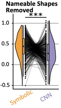
An identical analysis on the MEG leads to two noisy but significant clusters (CNN: 64.0ms to 172.0ms; then 192.0ms to 296.0ms; both p<.001: Geometric Features: 312.0ms to 364.0ms with p=.008). We have improved our manuscript thanks to the reviewer’s observation by adding a figure with the new behavior analysis to the supplementary figures and in the result section of the behavior task. We now refer to these analysis where appropriate:
(intro) “The effect appeared as a human universal, present in preschoolers, first-graders, and adults without access to formal western math education (the Himba from Namibia), and thus seemingly independent of education and of the existence of linguistic labels for regular shapes.”
(behavior results) “Finally, to separate the effect of name availability and geometric features on behavior, we replicated our analysis after removing the square, rectangle, trapezoids, rhombus and parallelogram from our data (Fig. S5D). This left us with five shapes, and an RDM with 10 entries, When regressing it in a GLM with our two models, we find that both models are still significant predictors (p<.001). The effect size of the geometric feature model is greatly reduced, yet remained significantly higher than that of the neural network model (p<.001).”
(meg results) “This analysis yielded similar clusters when performed on a subset of shapes that do not have an obvious name in English, as was the case for the behavior analysis (CNN Encoding: 64.0ms to 172.0ms; then 192.0ms to 296.0ms; both p<.001: Geometric Features: 312.0ms to 364.0ms with p=.008).”
(discussion, end of behavior section) “Previously, we only found such a significant mixture of predictors in uneducated humans (whether French preschoolers or adults from the Himba community, mitigating the possible impact of explicit western education, linguistic labels, and statistics of the environment on geometric shape representation) (Sablé-Meyer et al., 2021).”
Perhaps the referee’s point can also be reversed: we provide a normative theory of geometric shape complexity which has the potential to explain why certain shapes have names: instead of seeing shape names as the cause of their simpler mental representation, we suggest that the converse could occur, i.e. the simpler shapes are the ones that are given names.
(2) Task difficulty
On the other hand is the question of whether our effect is driven by task difficulty. First, we would like to point out that this point could apply to the fMRI task, which asks for an explicit detection of deviants, but does not apply to the MEG experiment. In MEG, participants passively looked at sequences of shapes which, for a given block, comprising many instances of a fixed standard shape and rare deviants–even if they notice deviants, they have no task related to them. Yet two independent findings validated the geometric features model: there was a large effect of geometric regularity on the MEG response to deviants, and the MEG dissimilarity matrix between standard shapes correlated with a model based on geometric features, better than with a model based on CNNs. While the response to rare deviants might perhaps be attributed to “difficulty” (assuming that, in spite of the absence of an explicit task, participants try to spot the deviants and find this self-imposed task more difficult in runs with less regular shapes), it seems very hard to explain the representational similarity analysis (RSA) findings based on difficulty. Indeed, what motivated us to use RSA analysis in both fMRI and MEG was to stop relying on the response to deviants, and use solely the data from standard or “reference” shapes, and model their neural response with theory-derived regressors.
We have updated the manuscript in several places to make our view on these points clearer:
(experiment 4) “This design allowed us to study the neural mechanisms of the geometric regularity effect without confounding effects of task, task difficulty, or eye movements.”
(figure 4, legend) “(A) Task structure: participants passively watch a constant stream of geometric shapes, one per second (presentation time 800ms). The stimuli are presented in blocks of 30 identical shapes up to scaling and rotation, with 4 occasional deviant shape. Participants do not have a task to perform beside fixating.”
Reviewer #2 (Public review):
Weakness:
Given that the primary take away from this study is that geometric shape information is found in the dorsal stream, rather than the ventral stream there is very little there is very little discussion of prior work in this area (for reviews, see Freud et al., 2016; Orban, 2011; Xu, 2018). Indeed, there is extensive evidence of shape processing in the dorsal pathway in human adults (Freud, Culham, et al., 2017; Konen & Kastner, 2008; Romei et al., 2011), children (Freud et al., 2019), patients (Freud, Ganel, et al., 2017), and monkeys (Janssen et al., 2008; Sereno & Maunsell, 1998; Van Dromme et al., 2016), as well as the similarity between models and dorsal shape representations (Ayzenberg & Behrmann, 2022; Han & Sereno, 2022).
We thank the reviewer for this opportunity to clarify our writing. We want to use this opportunity to highlight that our primary finding is not about whether the shapes of objects or animals (in general) are processed in the ventral versus or the dorsal pathway, but rather about the much more restricted domain of geometric shapes such as squares and triangles. We propose that simple geometric shapes afford additional levels of mental representation that rely on their geometric features – on top of the typical visual processing. To the best of our knowledge, this point has not been made in the above papers.
Still, we agree that it is useful to better link our proposal to previous ones. We have updated the discussion section titled “Two Visual Pathways” to include more specific references to the literature that have reported visual object representations in the dorsal pathway. Following another reviewer’s observation, we have also updated our analysis to better demonstrate the overlap in activation evoked by math and by geometry in the IPS, as well as include a novel comparison with independently published results.
Overall, to address this point, we (i) show the overlap between our “geometry” contrast (shape > word+tools+houses) and our “math” contrast (number > words); (ii) we display these ROIs side by side with ROIs found in previous work (Amalric and Dehaene, 2016), and (iii) in each math-related ROIs reported in that article, we test our “geometry” (shape > word+tools+houses) contrast and find almost all of them to be significant in both population; see Fig. S5.
Finally, within the ROIs identified with our geometry localizer, we also performed similarity analyses: for each region we extracted the betas of every voxel for every visual category, and estimated the distance (cross-validated mahalanobis) between different visual categories. In both ventral ROIs, in both populations, numbers were closer to shapes than to the other visual categories including text and Chinese characters (all p<.001). In adults, this result also holds for the right ITG (p=.021) and the left IPS (p=.014) but not the right IPS (p=.17). In children, this result did not hold in the areas.
Naturally, overlap in brain activation does not suffice to conclude that the same computational processes are involved. We have added an explicit caveat about this point. Indeed, throughout the article, we have been careful to frame our results in a way that is appropriate given our evidence, e.g. saying “Those areas are similar to those active during number perception, arithmetic, geometric sequences, and the processing of high-level math concepts” and “The IPS areas activated by geometric shapes overlap with those active during the comprehension of elementary as well as advanced mathematical concepts”. We have rephrased the possibly ambiguous “geometric shapes activated math- and number-related areas, particular the right aIPS.” into “geometric shapes activated areas independently found to be activated by math- and number-related tasks, in particular the right aIPS”.
Reviewer #3 (Public review):
Weakness:
Perhaps the manuscript could emphasize that the areas recruited by geometric figures but not objects are spatial, with reduced processing in visual areas. It also seems important to say that the images of real objects are interpreted as representations of 3D objects, as they activate the same visual areas as real objects. By contrast, the images of geometric forms are not interpreted as representations of real objects but rather perhaps as 2D abstractions.
This is an interesting possibility. Geometric shapes are likely to draw attention to spatial dimensions (e.g. length) and to do so in a 2D spatial frame of reference rather than the 3D representations evoked by most other objects or images. However, this possibility would require further work to be thoroughly evaluated, for instance by comparing usual 3D objects with rare instances of 2D ones (e.g. a sheet of paper, a sticker etc). In the absence of such a test, we refrained from further speculation on this point.
The authors use the term "symbolic." That use of that term could usefully be expanded here.
The reviewer is right in pointing out that “symbolic” should have been more clearly defined. We now added in the introduction:
(introduction) “[…] we sometimes refer to this model as “symbolic” because it relies on discrete, exact, rule-based features rather than continuous representations (Sablé-Meyer et al., 2022). In this representational format, geometric shapes are postulated to be represented by symbolic expressions in a “language-of-thought”, e.g. “a square is a four-sided figure with four equal sides and four right angles” or equivalently by a computer-like program from drawing them in a Logo-like language (Sablé-Meyer et al., 2022).”
Here, however, the present experiments do not directly probe this format of a representation. We have therefore simplified our wording and removed many of our use of the word “symbolic” in favor of the more specific “geometric features”.
Pigeons have remarkable visual systems. According to my fallible memory, Herrnstein investigated visual categories in pigeons. They can recognize individual people from fragments of photos, among other feats. I believe pigeons failed at geometric figures and also at cartoon drawings of things they could recognize in photos. This suggests they did not interpret line drawings of objects as representations of objects.
The comparison of geometric abilities across species is an interesting line of research. In the discussion, we briefly mention several lines of research that indicate that non-human primates do not perceive geometric shapes in the same way as we do – but for space reasons, we are reluctant to expand this section to a broader review of other more distant species. The referee is right that there is evidence of pigeons being able to perceive an invariant abstract 3D geometric shape in spite of much variation in viewpoint (Peissig et al., 2019) – but there does not seem to be evidence that they attend to geometric regularities specifically (e.g. squares versus non-squares). Also, the referee’s point bears on the somewhat different issue of whether humans and other animals may recognize the object depicted by a symbolic drawing (e.g. a sketch of a tree). Again, humans seem to be vastly superior in this domain, and research on this topic is currently ongoing in the lab. However, the point that we are making in the present work is specifically about the neural correlates of the representation of simple geometric shapes which by design were not intended to be interpretable as representations of objects.
Categories are established in part by contrast categories; are quadrilaterals, triangles, and circles different categories?
We are not sure how to interpret the referee’s question, since it bears on the definition of “category” (Spontaneous? After training? With what criterion?). While we are not aware of data that can unambiguously answer the reviewer’s question, categorical perception in geometric shapes can be inferred from early work investigating pop-out effects in visual search, e.g. (Treisman and Gormican, 1988): curvature appears to generate strong pop-out effects, and therefore we would expect e.g. circles to indeed be a different category than, say, triangles. Similarly, right angles, as well as parallel lines, have been found to be perceived categorically (Dillon et al., 2019).
This suggests that indeed squares would be perceived as categorically different from triangles and circles. On the other hand, in our own previous work (Sablé-Meyer et al., 2021) we have found that the deviants that we generated from our quadrilaterals did not pop out from displays of reference quadrilaterals. Pop-out is probably not the proper criterion for defining what a “category” is, but this is the extent to which we can provide an answer to the reviewer’s question.
It would be instructive to investigate stimuli that are on a continuum from representational to geometric, e.g., table tops or cartons under various projections, or balls or buildings that are rectangular or triangular. Building parts, inside and out. like corners. Objects differ from geometric forms in many ways: 3D rather than 2D, more complicated shapes, and internal texture. The geometric figures used are flat, 2-D, but much geometry is 3-D (e. g. cubes) with similar abstract features.
We agree that there is a whole line of potential research here. We decided to start by focusing on the simplest set of geometric shapes that would give us enough variation in geometric regularity while being easy to match on other visual features. We agree with the reviewer that our results should hold both for more complex 2-D shapes, but also for 3-D shapes. Indeed, generative theories of shapes in higher dimensions following similar principles as ours have been devised (I. Biederman, 1987; Leyton, 2003). We now mention this in the discussion:
“Finally, this research should ultimately be extended to the representation of 3-dimensional geometric shapes, for which similar symbolic generative models have indeed been proposed (Irving Biederman, 1987; Leyton, 2003).”
The feature space of geometry is more than parallelism and symmetry; angles are important, for example. Listing and testing features would be fascinating. Similarly, looking at younger or preferably non-Western children, as Western children are exposed to shapes in play at early ages.
We agree with the reviewer on all point. While we do not list and test the different properties separately in this work, we would like to highlight that angles are part of our geometric feature model, which includes features of “right-angle” and “equal-angles” as suggested by the reviewer.
We also agree about the importance of testing populations with limited exposure to formal training with geometric shapes. This was in fact a core aspect of a previous article of ours which tests both preschoolers, and adults with no access to formal western education – though no non-Western children (Sablé-Meyer et al., 2021). It remains a challenge to perform brain-imaging studies in non-Western populations (although see Dehaene et al., 2010; Pegado et al., 2014).
What in human experience but not the experience of close primates would drive the abstraction of these geometric properties? It's easy to make a case for elaborate brain processes for recognizing and distinguishing things in the world, shared by many species, but the case for brain areas sensitive to processing geometric figures is harder. The fact that these areas are active in blind mathematicians and that they are parietal areas suggests that what is important is spatial far more than visual. Could these geometric figures and their abstract properties be connected in some way to behavior, perhaps with fabrication and construction as well as use? Or with other interactions with complex objects and environments where symmetry and parallelism (and angles and curvature--and weight and size) would be important? Manual dexterity and fabrication also distinguish humans from great apes (quantitatively, not qualitatively), and action drives both visual and spatial representations of objects and spaces in the brain. I certainly wouldn't expect the authors to add research to this already packed paper, but raising some of the conceptual issues would contribute to the significance of the paper.
We refrained from speculating about this point in the previous version of the article, but share some of the reviewers’ intuitions about the underlying drive for geometric abstraction. As described in (Dehaene, 2026; Sablé-Meyer et al., 2022), our hypothesis, which isn’t tested in the present article, is that the emergence of a pervasive ability to represent aspects of the world as compact expressions in a mental “language-of-thought” is what underlies many domains of specific human competence, including some listed by the reviewer (tool construction, scene understanding) and our domain of study here, geometric shapes.
Recommendations for the Authors:
Reviewer #1 (Recommendations for the authors):
Overall, I enjoyed reading this paper. It is clearly written and nicely showcases the amount of work that has gone into conducting all these experiments and analyzing the data in sophisticated ways. I also thought the figures were great, and I liked the level of organization in the GitHub repository and am looking forward to seeing the shared data on OpenNeuro. I have some specific questions I hope the authors can address.
(1) Behavior
- Looking at Figure 1, it seemed like most shapes are clustering together, whereas square, rectangle, and maybe rhombus and parallelogram are slightly more unique. I was wondering whether the authors could comment on the potential influence of linguistic labels. Is it possible that it is easier to discard the intruder when the shapes are readily nameable versus not?
This is an interesting observation, but the existence of names for shapes does not suffice to explain all of our findings ; see our reply to the public comment.
(2) fMRI
- As mentioned in the public review, I was surprised that the authors went with an intruder task because I would imagine that performance depends on the specific combination of geometric shapes used within a trial. I assume it is much harder to find, for example, a "Right Hinge" embedded within "Hinge" stimuli than a "Right Hinge" amongst "Squares". In addition, the rotation and scaling of each individual item should affect regular shapes less than irregular shapes, creating visual dissimilarities that would presumably make the task harder. Can the authors comment on how we can be sure that the differences we pick up in the parietal areas are not related to task difficulty but are truly related to geometric shape regularities?
Again, please see our public review response for a larger discussion of the impact of task difficulty. There are two aspects to answering this question.
First, the task is not as the reviewer describes: the intruder task is to find a deviant shape within several slightly rotated and scaled versions of the regular shape it came from. During brain imaging, we did not ask participants to find an exemplar of one of our reference shape amidst copies of another, but rather a deviant version of one shape against copies of its reference version. We only used this intruder task with all pairs of shapes to generate the behavioral RSA matrix.
Second, we agree that some of the fMRI effect may stem from task difficulty, and this motivated our use of RSA analysis in fMRI, and a passive MEG task. RSA results cannot be explained by task difficulty.
Overall, we have tried to make the limitations of the fMRI design, and the motivation for turning to passive presentation in MEG, clearer by stating the issues more clearly when we introduce experiment 4:
“The temporal resolution of fMRI does not allow to track the dynamic of mental representations over time. Furthermore, the previous fMRI experiment suffered from several limitations. First, we studied six quadrilaterals only, compared to 11 in our previous behavioral work. Second, we used an explicit intruder detection, which implies that the geometric regularity effect was correlated with task difficulty, and we cannot exclude that this factor alone explains some of the activations in figure 3C (although it is much less clear how task difficulty alone would explain the RSA results in figure 3D). Third, the long display duration, which was necessary for good task performance especially in children, afforded the possibility of eye movements, which were not monitored inside the 3T scanner and again could have affected the activations in figure 3C.”
- How far in the periphery were the stimuli presented? Was eye-tracking data collected for the intruder task? Similar to the point above, I would imagine that a harder trial would result in more eye movements to find the intruder, which could drive some of the differences observed here.
A 1-degree bar was added to Figure 3A, which faithfully illustrates how the stimuli were presented in fMRI. Eye-tracking data was not collected during fMRI. Although the participants were explicitly instructed to fixate at the center of the screen and avoid eye movements, we fully agree with the referee that we cannot exclude that eye movements were present, perhaps more so for more difficult displays, and would therefore have contributed to the observed fMRI activations in experiment 3 (figure 3C). We now mention this limitation explicity at the end of experiment 3. However, crucially, this potential problem cannot apply to the MEG data. During the MEG task, the stimuli were presented one by one at the center of screen, without any explicit task, thus avoiding issues of eye movements. We therefore consider the MEG geometrical regularity effect, which comes at a relatively early latency (starting at ~160 ms) and even in a passive task, to provide the strongest evidence of geometric coding, unaffected by potential eye movement artefacts.
- I was wondering whether the authors would consider showing some un-thresholded maps just to see how widespread the activation of the geometric shapes is across all of the cortex.
We share the uncorrected threshold maps in Fig. S3. for both adults and children in the category localizer, copied here as well. For the geometry task, most of the clusters identified are fairly big and survive cluster-corrected permutations; the uncorrected statistical maps look almost fully identical to the one presented in Fig. 3 (p<.001 map).
- I'm missing some discussion on the role of early visual areas that goes beyond the RSA-CNN comparison. I would imagine that early visual areas are not only engaged due to top-down feedback (line 258) but may actually also encode some of the geometric features, such as parallel lines and symmetry. Is it feasible to look at early visual areas and examine what the similarity structure between different shapes looks like?
If early visual areas encoded the geometric features that we propose, then even early sensor-level RSA matrices should show a strong impact of geometric features similarity, which is not what we find (figure 4D). We do, however, appreciate the referee’s request to examine more closely how this similarity structure looks like. We now provide a movie showing the significant correlation between neural activity and our two models (uncorrected participants); indeed, while the early occipital activity (around 110ms) is dominated by a significant correlation with the CNN model, there are also scattered significant sources associated to the symbolic model around these timepoints already.
To test this further, we used beamformers to reconstruct the source-localized activity in calcarine cortex and performed an RSA analysis across that ROI. We find that indeed the CNN model is strongly significant at t=110ms (t=3.43, df=18, p=.003) while the geometric feature model is not (t=1.04, df=18, p=.31), and the CNN is significantly above the geometric feature model (t=4.25, df=18, p<.001). However, this result is not very stable across time, and there are significant temporal clusters around these timepoints associated to each model, with no significant cluster associated to a CNN > geometric (CNN: significant cluster from 88ms to 140ms, p<.001 in permutation based with 10000 permutations; geometric features has a significant cluster from 80ms to 104ms, p=.0475; no significant cluster on the difference between the two).
(3) MEG
- Similar to the fMRI set, I am a little worried that task difficulty has an effect on the decoding results, as the oddball should pop out more in more geometric shapes, making it easier to detect and easier to decode. Can the authors comment on whether it would matter for the conclusions whether they are decoding varying task difficulty or differences in geometric regularity, or whether they think this can be considered similarly?
See above for an extensive discussion of the task difficulty effect. We point out that there is no task in the MEG data collection part. We have clarified the task design by updating our Fig. 4. Additionally, the fact that oddballs are more perceived more or less easily as a function of their geometric regularity is, in part, exactly the point that we are making – but, in MEG, even in the absence of a task of looking for them.
- The authors discuss that the inflated baseline/onset decoding/regression estimates may occur because the shapes are being repeated within a mini-block, which I think is unlikely given the long ISIs and the fact that the geometric features model is not >0 at onset. I think their second possible explanation, that this may have to do with smoothing, is very possible. In the text, it said that for the non-smoothed result, the CNN encoding correlates with the data from 60ms, which makes a lot more sense. I would like to encourage the authors to provide readers with the unsmoothed beta values instead of the 100-ms smoothed version in the main plot to preserve the reason they chose to use MEG - for high temporal resolution!
We fully agree with the reviewer and have accordingly updated the figures to show the unsmoothed data (see below). Indeed, there is now no significant CNN effect before ~60 ms (up to the accuracy of identifying onsets with our method).
- In Figure 4C, I think it would be useful to either provide error bars or show variability across participants by plotting each participant's beta values. I think it would also be nice to plot the dissimilarity matrices based on the MEG data at select timepoints, just to see what the similarity structure is like.
Following the reviewer’s recommendation, we plot the timeseries with SEM as shaded area, and thicker lines for statistically significant clusters, and we provide the unsmoothed version in figure Fig. 4. As for the dissimilarity matrices at select timepoints, this has now been added to figure Fig. 4.
- To evaluate the source model reconstruction, I think the reader would need a little more detail on how it was done in the main text. How were the lead fields calculated? Which data was used to estimate the sources? How are the models correlated with the source data?
We have imported some of the details in the main text as follows (as well as expanding the methods section a little):
“To understand which brain areas generated these distinct patterns of activations, and probe whether they fit with our previous fMRI results, we performed a source reconstruction of our data. We projected the sensor activity onto each participant's cortical surfaces estimated from T1-images. The projection was performed using eLORETA and emptyroom recordings acquired on the same day to estimate noise covariance, with the default parameters of mne-bids-pipeline. Sources were spaced using a recursively subdivided octahedron (oct5). Group statistics were performed after alignement to fsaverage. We then replicated the RSA analysis […]”
- In addition to fitting the CNN, which is used here to model differences in early visual cortex, have the authors considered looking at their fMRI results and localizing early visual regions, extracting a similarity matrix, and correlating that with the MEG and/or comparing it with the CNN model?
We had ultimately decided against comparing the empirical similarity matrices from the MEG and fMRI experiments, first because the stimuli and tasks are different, and second because this would not be directly relevant to our goal, which is to evaluate whether a geometric-feature model accounts for the data. Thus, we systematically model empirical similarity matrices from fMRI and from MEG with our two models derived from different theories of shape perception in order to test predictions about their spatial and temporal dynamic. As for comparing the similarity matrix from early visual regions in fMRI with that predicted by the CNN model, this is effectively visible from our Fig. 3D where we perform searchlight RSA analysis and modeling with both the CNN and the geometric feature model; bilaterally, we find a correlation with the CNN model, although it sometimes overlap with predictions from the geometric feature model as well. We now include a section explaining this reasoning in appendix:
“Representational similarity analysis also offers a way to directly compared similarity matrices measured in MEG and fMRI, thus allowing for fusion of those two modalities and tentatively assigning a “time stamp” to distinct MRI clusters. However, we did not attempt such an analysis here for several reasons. First, distinct tasks and block structures were used in MEG and fMRI. Second, a smaller list of shapes was used in fMRI, as imposed by the slower modality of acquisition. Third, our study was designed as an attempt to sort out between two models of geometric shape recognition. We therefore focused all analyses on this goal, which could not have been achieved by direct MEG-fMRI fusion, but required correlation with independently obtained model predictions.”
Minor comments
- It's a little unclear from the abstract that there is children's data for fMRI only.
We have reworded the abstract to make this unambiguous
- Figures 4a & b are missing y-labels.
We can see how our labels could be confused with (sub-)plot titles and have moved them to make the interpretation clearer.
- MEG: are the stimuli always shown in the same orientation and size?
They are not, each shape has a random orientation and scaling. On top of a task example at the top of Fig. 4, we have now included a clearer mention of this in the main text when we introduce the task:
“shapes were presented serially, one at a time, with small random changes in rotation and scaling parameters, in miniblocks with a fixed quadrilateral shape and with rare intruders with the bottom right corner shifted by a fixed amount (Sablé-Meyer et al., 2021)”
- To me, the discussion section felt a little lengthy, and I wonder whether it would benefit from being a little more streamlined, focused, and targeted. I found that the structure was a little difficult to follow as it went from describing the result by modality (behavior, fMRI, MEG) back to discussing mostly aspects of the fMRI findings.
We have tried to re-organize and streamline the discussion following these comments.
Then, later on, I found that especially the section on "neurophysiological implementation of geometry" went beyond the focus of the data presented in the paper and was comparatively long and speculative.
We have reexamined the discussion, but the citation of papers emphasizing a representation of non-accidental geometric properties in non-human animals was requested by other commentators on our article; and indeed, we think that they are relevant in the context of our prior suggestion that the composition of geometric features might be a uniquely human feature – these papers suggest that individual features may not, and that it is therefore compositionality which might be special to the human brain. We have nevertheless shortened it.
Furthermore, we think that this section is important because symbolic models are often criticized for lack of a plausible neurophysiological implementation. It is therefore important to discuss whether and how the postulated symbolic geometric code could be realized in neural circuits. We have added this justification to the introduction of this section.
Reviewer #2 (Recommendations for the authors):
(1) If the authors want to specifically claim that their findings align with mathematical reasoning, they could at least show the overlap between the activation maps of the current study and those from prior work.
This was added to the fMRI results. See our answers to the public review.
(2) I wonder if the reason the authors only found aIPS in their first analysis (Figure 2) is because they are contrasting geometric shapes with figures that also have geometric properties. In other words, faces, objects, and houses also contain geometric shape information, and so the authors may have essentially contrasted out other areas that are sensitive to these features. One indication that this may be the case is that the geometric regularity effect and searchlight RSA (Figure 3) contains both anterior and posterior IPS regions (but crucially, little ventral activity). It might be interesting to discuss the implications of these differences.
Indeed, we cannot exclude that the few symmetries, perpendicularity and parallelism cues that can be presented in faces, objects or houses were processed as such, perhaps within the ventral pathway, and that these representations would have been subtracted out. We emphasize that our subtraction isolates the geometrical features that are present in simple regular geometric shapes, over and above those that might exist in other categories. We have added this point to the discussion:
“[… ] For instance, faces possess a plane of quasi-symmetry, and so do many other man-made tools and houses. Thus, our subtraction isolated the geometrical features that are present in simple regular geometric shapes (e.g. parallels, right angles, equality of length) over and above those that might already exist, in a less pure form, in other categories.”
(3) I had a few questions regarding the MEG results.
a. I didn't quite understand the task. What is a regular or oddball shape in this context? It's not clear what is being decoded. Perhaps a small example of the MEG task in Figure 4 would help?
We now include an additional sub-figure in Fig. 4 to explain the paradigm. In brief: there is no explicit task, participants are simply asked to fixate. The shapes come in miniblocks of 30 identical reference shapes (up to rotation and scaling), among which some occasional deviant shapes randomly appear (created by moving the corner of the reference shape by some amount).
b. In Figure 4A/B they describe the correlation with a 'symbolic model'. Is this the same as the geometric model in 4C?
It is. We have removed this ambiguity by calling it “geometric model” and setting its color to the one associated to this model thought the article.
c. The author's explanation for why geometric feature coding was slower than CNN encoding doesn't quite make sense to me. As an explanation, they suggest that previous studies computed "elementary features of location or motor affordance", whereas their study work examines "high-level mathematical information of an abstract nature." However, looking at the studies the authors cite in this section, it seems that these studies also examined the time course of shape processing in the dorsal pathway, not "elementary features of location or motor affordance." Second, it's not clear how the geometric feature model reflects high-level mathematical information (see point above about claiming this is related to math).
We thank the referee for pointing out this inappropriate phrase, which we removed. We rephrased the rest of the paragraph to clarify our hypothesis in the following way:
“However, in this work, we specifically probed the processing of geometric shapes that, if our hypothesis is correct, are represented as mental expressions that combine geometrical and arithmetic features of an abstract categorical nature, for instance representing “four equal sides” or “four right angles”. It seems logical that such expressions, combining number, angle and length information, take more time to be computed than the first wave of feedforward processing within the occipito-temporal visual pathway, and therefore only activate thereafter.”
One explanation may be that the authors' geometric shapes require finer-grained discrimination than the object categories used in prior studies. i.e., the odd-ball task may be more of a fine-grained visual discrimination task. Indeed, it may not be a surprise that one can decode the difference between, say, a hammer and a butterfly faster than two kinds of quadrilaterals.
We do not disagree with this intuition, although note that we do not have data on this point (we are reporting and modelling the MEG RSA matrix across geometric shapes only – in this part, no other shapes such as tools or faces are involved). Still, the difference between squares, rectangles, parallelograms and other geometric shapes in our stimuli is not so subtle. Furthermore, CNNs do make very fine grained distinctions, for instance between many different breeds of dogs in the IMAGENET corpus. Still, those sorts of distinctions capture the initial part of the MEG response, while the geometric model is needed only for the later part. Thus, we think that it is a genuine finding that geometric computations associated with the dorsal parietal pathway are slower than the image analysis performed by the ventral occipito-temporal pathway.
d. CNN encoding at time 0 is a little weird, but the author's explanation, that this is explained by the fact that temporal smoothed using a 100 ms window makes sense. However, smoothing by 100 ms is quite a lot, and it doesn't seem accurate to present continuous time course data when the decoding or RSA result at each time point reflects a 100 ms bin. It may be more accurate to simply show unsmoothed data. I'm less convinced by the explanation about shape prediction.
We agree. Following the reviewer’s advice, as well as the recommendation from reviewer 1, we now display unsmoothed plots, and the effects now exhibit a more reasonable timing (Figure 4D), with effects starting around ~60 ms for CNN encoding.
(4) I appreciate the author's use of multiple models and their explanation for why DINOv2 explains more variance than the geometric and CNN models (that it represents both types of features. A variance partitioning analysis may help strengthen this conclusion (Bonner & Epstein, 2018; Lescroart et al., 2015).
However, one difference between DINOv2 and the CNN used here is that it is trained on a dataset of 142 million images vs. the 1.5 million images used in ImageNet. Thus, DINOv2 is more likely to have been exposed to simple geometric shapes during training, whereas standard ImageNet trained models are not. Indeed, prior work has shown that lesioning line drawing-like images from such datasets drastically impairs the performance of large models (Mayilvahanan et al., 2024). Thus, it is unlikely that the use of a transformer architecture explains the performance of DINOv2. The authors could include an ImageNet-trained transformer (e.g., ViT) and a CNN trained on large datasets (e.g., ResNet trained on the Open Clip dataset) to test these possibilities. However, I think it's also sufficient to discuss visual experience as a possible explanation for the CNN and DINOv2 results. Indeed, young children are exposed to geometric shapes, whereas ImageNet-trained CNNs are not.
We agree with the reviewer’s observation. In fact, new and ongoing work from the lab is also exploring this; we have included in supplementary materials exactly what the reviewer is suggesting, namely the time course of the correlation with ViT and with ConvNeXT. In line with the reviewers’ prediction, these networks, trained on much larger dataset and with many more parameters, can also fit the human data as well as DINOv2. We ran additional analysis of the MEG data with ViT and ConvNeXT, which we now report in Fig. S6 as well as in an additional sentence in that section:
“[…] similar results were obtained by performing the same analysis, not only with another vision transformer network, ViT, but crucially using a much larger convolutional neural network, ConvNeXT, which comprises ~800M parameters and has been trained on 2B images, likely including many geometric shapes and human drawings. For the sake of completeness, RSA analysis in sensor space of the MEG data with these two models is provided in Fig. S6.”
We conclude that the size and nature of the training set could be as important as the architecture – but also note that humans do not rely on such a huge training set. We have updated the text, as well as Fig. S6, accordingly by updating the section now entitled “Vision Transformers and Larger Neural Networks”, and the discussion section on theoretical models.
(5) The authors may be interested in a recent paper from Arcaro and colleagues that showed that the parietal cortex is greatly expanded in humans (including infants) compared to non-human primates (Meyer et al., 2025), which may explain the stronger geometric reasoning abilities of humans.
A very interesting article indeed! We have updated our article to incorporate this reference in the discussion, in the section on visual pathways, as follows:
“Finally, recent work shows that within the visual cortex, the strongest relative difference in growth between human and non-human primates is localized in parietal areas (Meyer et al., 2025). If this expansion reflected the acquisition of new processing abilities in these regions, it might explain the observed differences in geometric abilities between human and non-human primates (Sablé-Meyer et al., 2021).”
Also, the authors may want to include this paper, which uses a similar oddity task and compelling shows that crows are sensitive to geometric regularity:
Schmidbauer, P., Hahn, M., & Nieder, A. (2025). Crows recognize geometric regularity. Science Advances, 11(15), eadt3718. https://doi.org/10.1126/sciadv.adt3718
We have ongoing discussions with the authors of this work and are have prepared a response to their findings (Sablé-Meyer and Dehaene, 2025)–ultimately, we think that this discussion, which we agree is important, does not have its place in the present article. They used a reduced version of our design, with amplified differences in the intruders. While they did not test the fit of their model with CNN or geometric feature models, we did and found that a simple CNN suffices to account for crow behavior. Thus, we disagree that their conclusions follow from their results and their conclusions. But the present article does not seem to be the right platform to engage in this discussion.
References
Ayzenberg, V., & Behrmann, M. (2022). The Dorsal Visual Pathway Represents Object-Centered Spatial Relations for Object Recognition. The Journal of Neuroscience, 42(23), 4693-4710. https://doi.org/10.1523/jneurosci.2257-21.2022
Bonner, M. F., & Epstein, R. A. (2018). Computational mechanisms underlying cortical responses to the affordance properties of visual scenes. PLoS Computational Biology, 14(4), e1006111. https://doi.org/10.1371/journal.pcbi.1006111
Bueti, D., & Walsh, V. (2009). The parietal cortex and the representation of time, space, number and other magnitudes. Philosophical Transactions of the Royal Society B: Biological Sciences, 364(1525), 1831-1840.
Dehaene, S., & Brannon, E. (2011). Space, time and number in the brain: Searching for the foundations of mathematical thought. Academic Press.
Freud, E., Culham, J. C., Plaut, D. C., & Bermann, M. (2017). The large-scale organization of shape processing in the ventral and dorsal pathways. eLife, 6, e27576.
Freud, E., Ganel, T., Shelef, I., Hammer, M. D., Avidan, G., & Behrmann, M. (2017). Three-dimensional representations of objects in dorsal cortex are dissociable from those in ventral cortex. Cerebral Cortex, 27(1), 422-434.
Freud, E., Plaut, D. C., & Behrmann, M. (2016). 'What 'is happening in the dorsal visual pathway. Trends in Cognitive Sciences, 20(10), 773-784.
Freud, E., Plaut, D. C., & Behrmann, M. (2019). Protracted developmental trajectory of shape processing along the two visual pathways. Journal of Cognitive Neuroscience, 31(10), 1589-1597.
Han, Z., & Sereno, A. (2022). Modeling the Ventral and Dorsal Cortical Visual Pathways Using Artificial Neural Networks. Neural Computation, 34(1), 138-171. https://doi.org/10.1162/neco_a_01456
Janssen, P., Srivastava, S., Ombelet, S., & Orban, G. A. (2008). Coding of shape and position in macaque lateral intraparietal area. Journal of Neuroscience, 28(26), 6679-6690.
Konen, C. S., & Kastner, S. (2008). Two hierarchically organized neural systems for object information in human visual cortex. Nature Neuroscience, 11(2), 224-231.
Lescroart, M. D., Stansbury, D. E., & Gallant, J. L. (2015). Fourier power, subjective distance, and object categories all provide plausible models of BOLD responses in scene-selective visual areas. Frontiers in Computational Neuroscience, 9(135), 1-20. https://doi.org/10.3389/fncom.2015.00135
Mayilvahanan, P., Zimmermann, R. S., Wiedemer, T., Rusak, E., Juhos, A., Bethge, M., & Brendel, W. (2024). In search of forgotten domain generalization. arXiv Preprint arXiv:2410.08258.
Meyer, E. E., Martynek, M., Kastner, S., Livingstone, M. S., & Arcaro, M. J. (2025). Expansion of a conserved architecture drives the evolution of the primate visual cortex. Proceedings of the National Academy of Sciences, 122(3), e2421585122. https://doi.org/10.1073/pnas.2421585122
Orban, G. A. (2011). The extraction of 3D shape in the visual system of human and nonhuman primates. Annual Review of Neuroscience, 34, 361-388.
Romei, V., Driver, J., Schyns, P. G., & Thut, G. (2011). Rhythmic TMS over Parietal Cortex Links Distinct Brain Frequencies to Global versus Local Visual Processing. Current Biology, 21(4), 334-337. https://doi.org/10.1016/j.cub.2011.01.035
Sereno, A. B., & Maunsell, J. H. R. (1998). Shape selectivity in primate lateral intraparietal cortex. Nature, 395(6701), 500-503. https://doi.org/10.1038/26752
Summerfield, C., Luyckx, F., & Sheahan, H. (2020). Structure learning and the posterior parietal cortex. Progress in Neurobiology, 184, 101717. https://doi.org/10.1016/j.pneurobio.2019.101717
Van Dromme, I. C., Premereur, E., Verhoef, B.-E., Vanduffel, W., & Janssen, P. (2016). Posterior Parietal Cortex Drives Inferotemporal Activations During Three-Dimensional Object Vision. PLoS Biology, 14(4), e1002445. https://doi.org/10.1371/journal.pbio.1002445
Xu, Y. (2018). A tale of two visual systems: Invariant and adaptive visual information representations in the primate brain. Annu. Rev. Vis. Sci, 4, 311-336.
Reviewer #3 (Recommendations for the authors):
Bring into the discussion some of the issues outlined above, especially a) the spatial rather than visual of the geometric figures and b) the non-representational aspects of geometric form aspects.
We thank the reviewer for their recommendations – see our response to the public review for more details.
-
-
www.biorxiv.org www.biorxiv.org
-
Author Response
Reviewer #1 (Public Review):
In this manuscript, Goering et al. investigate subcellular RNA localization across different cell types focusing on epithelial cells (mouse C2bbe1 and human HCA-7 enterocyte monolayers, canine MDCK epithelial cells) as well as neuronal cultures (mouse CAD cells). They use their recently established Halo-seq method to investigate transcriptome-wide RNA localization biases in C2bbe1 enterocyte monolayers and find that 5'TOP-motif containing mRNAs, which encode ribosomal proteins (RPs), are enriched on the basal side of these cells. These results are supported by smFISH against endogenous RP-encoding mRNAs (RPL7 and RPS28) as well as Firefly luciferase reporter transcripts with and without mutated 5'TOP sequences. Furthermore, they find that 5'TOP-motifs are not only driving localization to the basal side of epithelial cells but also to neuronal processes. To investigate the molecular mechanism behind the observed RNA localization biases, they reduce expression of several Larp proteins and find that RNA localization is consistently Larp1-dependent. Additionally, the localization depends on the placement of the TOP sequence in the 5'UTR and not the 3'UTR. To confirm that similar RNA localization biases can be conserved across cell types for other classes of transcripts, they perform similar experiments with a GA-rich element containing Net1 3'UTR transcript, which has previously been shown to exhibit a strong localization bias in several cell types. In order to determine if motor proteins contribute to these RNA distributions, they use motor protein inhibitors to confirm that the localization of individual members of both classes of transcripts, 5'TOP and GA-rich, is kinesin-dependent and that RNA localization to specific subcellular regions is likely to coincide with RNA localization to microtubule plus ends that concentrate in the basal side of epithelial cells as well as in neuronal processes.
In summary, Goering et al. present an interesting study that contributes to our understanding of RNA localization. While RNA localization has predominantly been studied in a single cell type or experimental system, this work looks for commonalities to explain general principles. I believe that this is an important advance, but there are several points that should be addressed.
Comments:
1) The Mili lab has previously characterized the localization of ribosomal proteins and NET1 to protrusions (Wang et al, 2017, Moissoglu et al 2019, Crisafis et al., 2020) and the role of kinesins in this localization (Pichon et al, 2021). These papers should be cited and their work discussed. I do not believe this reduces the novelty of this study and supports the generality of the RNA localization patterns to additional cellular locations in other cell types.
This was an unintentional oversight on our part, and we apologize. We have added citations for the mentioned publications and discussed our work in the context of theirs.
2) The 5'TOP motif begins with an invariant C nucleotide and mutation of this first nucleotide next to the cap has been shown to reduce translation regulation during mTOR inhibition (Avni et al, 1994 and Biberman et al 1997) and also Lapr1 binding (Lahr et al, 2017). Consequently, it is not clear to me if RPS28 initiates transcription with an A as indicated in Figure 3B. There also seems to be some differences in published CAGE datasets, but this point needs to be clarified. Additionally, it is not clear to me how the 5'TOP Firefly luciferase reporters were generated and if the transcription start site and exact 5'-ends of these constructs were determined. This is again essential to determine if it is a pyrimidine sequence in the 5'UTR that is important for localization or the 5'TOP motif and if Larp1 is directly regulating the localization by binding to the 5'TOP motif or if the effect they observe is indirect (e.g. is Larp1 also basally localized?). It should also be noted that Larp1 has been suggested to bind pyrimidine-rich sequences in the 5'UTR that are not next to the cap, but the details of this interaction are less clear (Al-Ashtal et al, 2021)
We did not fully appreciate the subtleties related to TOP motif location when we submitted this manuscript, so we thank the reviewer for pointing them out.
We also analyzed public CAGE datasets (Andersson et al, 2014 Nat Comm) and found that the start sites for both RPL7 and RPS28 were quite variable within a window of several nucleotides (as is the case for the vast majority of genes), suggesting that a substantial fraction of both do not begin with pyrimidines (Reviewer Figure 1). Yet, by smFISH, endogenous RPL7 and RPS28 are clearly basally/neurite localized (see new figure 3C).
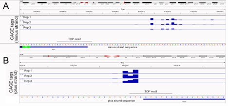
Reviewer Figure 1. Analysis of transcription start sites for RPL7 (A) and RPS28 (B) using CAGE data (Andersson et al, 2014 Nat Comm). Both genes show a window of transcription start sites upstream of current gene models (blue bars at bottom).
A more detailed analysis of our PRRE-containing reporter transcripts led us to find that in these reporters, the pyrimidine-rich element was approximately 90 nucleotides into the body of the 5’ UTR. Yet these reporters are also basally/neurite localized. The organization of the PRRE-containing reporters is now more clearly shown in an updated figure 3D.
From these results, it would seem that the pyrimidine-rich element need not be next to the 5’ cap in order to regulate RNA localization. To generalize this result, we first used previously identified 5’ UTR pyrimidine-rich elements that had been found to regulate translation in an mTOR-dependent manner (Hsieh et al 2012). We found that, as a class, RNAs containing these motifs were similarly basally/neurite localized as RP mRNAs. These results are presented in figures 3A and 3I.
We then asked if the position of the pyrimidine-rich element within the 5’ UTR of these RNAs was related to their localization. We found no relationship between element position and transcript localization as elements within the bodies of 5’ UTRs were seemingly just as able to promote basal/neurite localization as elements immediately next to the 5’ cap. These results are presented in figures 3B and 3J.
To further confirm that pyrimidine-rich elements need not be immediately next to the 5’ cap, we redesigned our RPL7-derived reporter transcripts such that the pyrimidine-rich motif was immediately adjacent to the 5’ cap. This was possible because the reporter uses a CMV promoter that reliably starts transcription at a known nucleotide. We then compared the localization of this reporter (called “RPL7 True TOP”) to our previous reporter in which the pyrimidine-rich element was ~90 nt into the 5’ UTR (called “RPL7 PRRE”) (Reviewer Figure 2). As with the PRRE reporter, the True TOP reporter drove RNA localization in both epithelial and neuronal cells while purine-containing mutant versions of the True TOP reporter did not (Reviewer Figure 2A-D). In the epithelial cells, the True TOP was modestly but significantly better at driving basal RNA localization than the PRRE (Reviewer Figure 2E) while in neuronal cells the True TOPs were modestly but insignificantly better. Again, this suggests that pyrimidine-rich motifs need not be immediately cap-adjacent in order to regulate RNA localization.
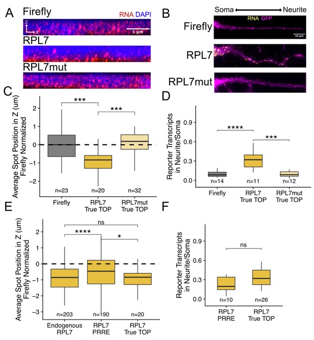
Reviewer Figure 2. Experimental confirmation that pyrimidine-rich motif location within 5’ UTRs is not critical for RNA localization. (A) RPL7 True TOP smFISH in epithelial cells. (B) RPL7 True TOP smFISH in neuronal cells. (C) Quantification of epithelial cell smFISH in A. (D) Quantification of neuronal cell smFISH in D. (E) Comparison of the location in epithelial cells of endogenous RPL7 transcripts, RPL7 PRRE reporter transcripts, and PRL7 True TOP reporter transcripts. (F) Comparison of the neurite-enrichment of RPL7 PRRE reporters and RPL7 True TOP reporters. In C-F, the number of cells included in each analysis is shown.
In response to the point about whether the localization results are direct effects of LARP1, we did not assay the binding of LARP1 to our PRRE-containing reporters, so we cannot say for sure. However, given that PRRE-dependent localization required LARP1 and there is much evidence about LARP1 binding pyrimidine-rich elements (including those that are not cap-proximal as the reviewer notes), we believe this to be the most likely explanation.
It should also be noted here that while pyrimidine-rich motif position within the 5’ UTR may not matter, its location within the transcript does. PRREs located within 3’ UTRs were unable to direct RNA localization (Figure 5).
3) In figure 1A, they indicate that mRNA stability can contribute to RNA localization, but this point is never discussed. This may be important to their work since Larp1 has also been found to impact mRNA half-lives (Aoki et al, 2013 and Mattijssen et al 2020, Al-Ashtal et al 2021). Is it possible the effect they see when Larp1 is depleted comes from decreased stability?
We found that PRRE-containing reporter transcripts were generally less abundant than their mutant counterparts in C2bbe1, HCA7, and MDCK cells (figure 3 – figure supplements 5, 6, and 8) although the effect was not consistent in mouse neuronal cells (figure 3 – figure supplement 13).
However, we don’t think it is likely that the changes in localization are due to stability changes. This abundance effect did not seem to be LARP1-dependent as both PRRE-containing and PRRE-mutant reporters were generally more expressed in LARP1-rescue epithelial cells than in LARP1 KO cells (figure 4 – figure supplement 9).
It should be noted here that we are not ever actually measuring transcript stability but rather steady state abundances. It cannot therefore be ruled out that LARP1 is regulating the stability of our PRRE reporters. Given, though, that their localization was dependent on kinesin activity (figures 7F, 7G), we believe the most likely explanation for the localization effects is active transport.
4) Also Moor et al, 2017 saw that feeding cycles changed the localization of 5'TOP mRNAs. Similarly, does mTOR inhibition or activation or simply active translation alter the localization patterns they observe? Further evidence for dynamic regulation of RNA localization would strengthen this paper
We are very interested in this and have begun exploring it. We have data suggesting that PRREs also mediate the feeding cycle-dependent relocalization of RP mRNAs. As the reviewer says, we think this leads to a very attractive model involving mTOR, and we are currently working to test this model. However, we don’t have the room to include those results in this manuscript and would instead prefer to include them in a later manuscript that focuses on nutrient-induced dynamic relocalization.
5) For smFISH quantification, is every mRNA treated as an independent measurement so that the statistics are calculated on hundreds of mRNAs? Large sample sizes can give significant p-values but have very small differences as observe for Firefly vs. OSBPL3 localization. Since determining the biological interpretation of effect size is not always clear, I would suggest plotting RNA position per cell or only treat biological replicates as independent measurements to determine statistical significance. This should also be done for other smFISH comparisons
This is a good suggestion, and we agree that using individual puncta as independent observations will artificially inflate the statistical power in the experiment. To remedy this in the epithelial cell images, we first reanalyzed the smFISH images using each of the following as a unique observation: the mean location of all smFISH puncta in one cell, the mean location of all puncta in a field of view, and the mean location of all puncta in one coverslip. With each metric, the results we observed were very similar (Reviewer Figure 3) while the statistical power of course decreased. We therefore chose to go with the reviewer-suggested metric of mean transcript position per cell.
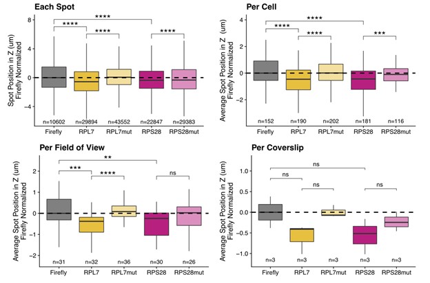
Reviewer Figure 3. C2bbe1 monolayer smFISH spot position analysis. RNA localization across the apicobasal axis is measured by smFISH spot position in the Z axis. This can be plotted for each spot, where thousands of spots over-power the statistics. Spot position can be averaged per cell as outlined manually within the FISH-quant software. This reduces sample size and allows for more accurate statistical analysis. When spot position is averaged per field of view, sample size further decreases, statistics are less powered but the localization trends are still robust. Finally, we can average spot position per coverslip, which represents biological replicates. We lose almost all statistical power as sample size is limited to 3 coverslips. Despite this, the localization trends are still recognizable.
When we use this metric, all results remain the same with the exception of the smFISH validation of endogenous OSBPL3 localization. That result loses its statistical significance and has now been omitted from the manuscript. All epithelial smFISH panels have been updated to use this new metric, and the number of cells associated with each observation is indicated for each sample.
For the neuronal images, these were already quantified at the per-cell level as we compare soma and neurite transcript counts from the same cell. In lieu of more imaging of these samples, we chose to perform subcellular fractionation into soma and neurite samples followed by RT-qPCR as an orthogonal technique (figure 3K, figure 3 supplement 14). This technique profiles the population average of approximately 3 million cells.
6) F: How was the segmentation of soma vs. neurites performed? It would be good to have a larger image as a supplemental figure so that it is clear the proximal or distal neurites segments are being compared
All neurite vs. soma segmentations were done manually. An example of this segmentation is included as Reviewer Figure 4. This means that often only proximal neurites segments are included in the analysis as it is often difficult to find an entire soma and an entire neurite in one field of view. However, in our experience, inclusion of more distal neurite segments would likely only strengthen the smFISH results as we often observe many molecules of localized transcripts in the distal tips of these neurites.
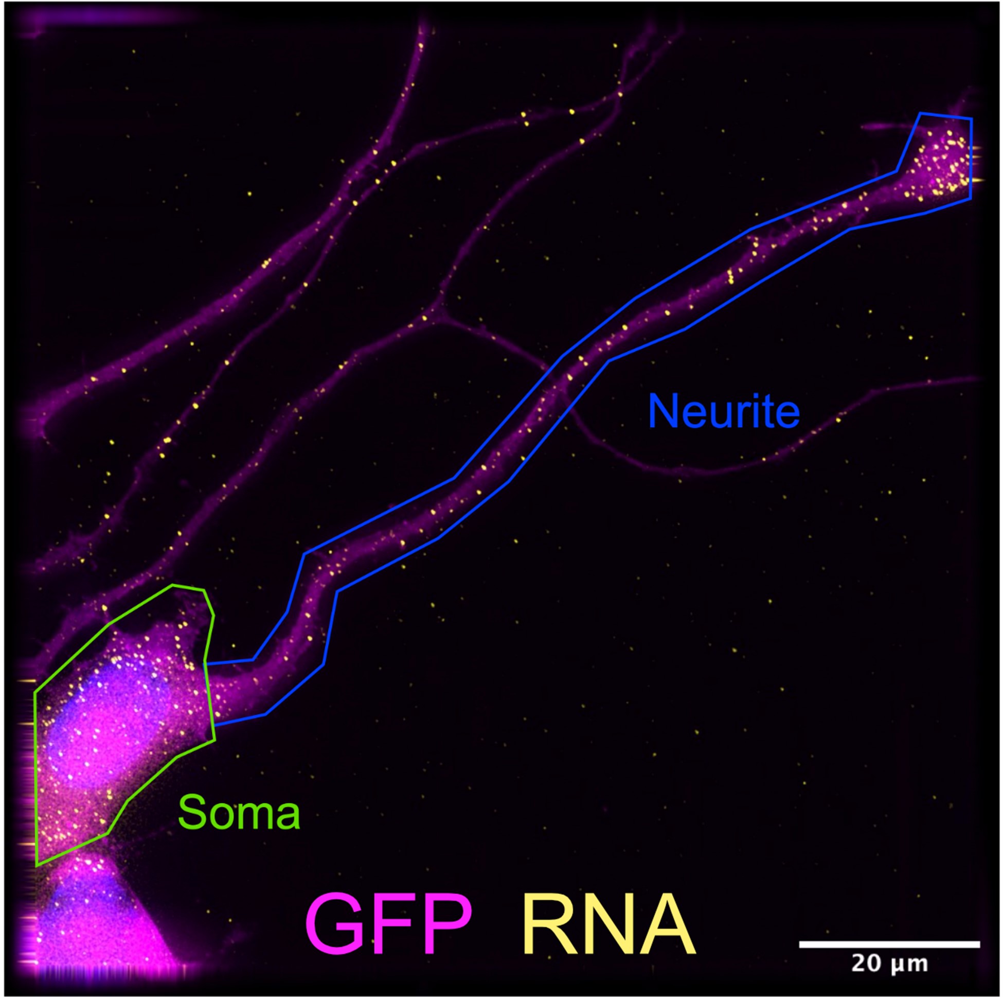
Reviewer Figure 4. Manual segmentation of differentiated CAD soma and neurite in FISH-quant software. Neurites that do not overlap adjacent neurites are selected for imaging. Often neurites extend beyond the field of view, limiting this assay to RNA localization in proximal neurites.
Also, it should be noted that the neuronal smFISH results are now supplemented by experiments involving subcellular fractionation and RT-qPCR (figure 3 supplement 14). These subcellular fractionation experiments collect the whole neurite, both the proximal and distal portions.
Text has been added to the methods under the header “smFISH computational analysis” to clarify how the segmentation was done.
-
-
www.biorxiv.org www.biorxiv.org
-
Author response:
The following is the authors’ response to the original reviews.
Reviewer #1 (Public review):
Strengths:
Sarpaning et al. provide a thorough characterization of putative Rnt1 cleavage of mRNA in S. cerevisiae. Previous studies have discovered Rnt1 mRNA substrates anecdotally, and this global characterization expands the known collection of putative Rnt1 cleavage sites. The study is comprehensive, with several types of controls to show that Rnt1 is required for several of these cleavages.
Weaknesses:
(1) Formally speaking, the authors do not show a direct role of Rnt1 in mRNA cleavage - no studies were done (e.g., CLIP-seq or similar) to define direct binding sites. Is the mutant Rnt1 expected to trap substrates? Without direct binding studies, the authors rely on genetics and structure predictions for their argument, and it remains possible that a subset of these sites is an indirect consequence of rnt1. This aspect should be addressed in the discussion.
We have added to this point in the discussion, as requested. We do not, however, agree that CLIP-seq or other methods are needed to address this point, or would even be helpful in the question the reviewer raises.
Importantly, we show that recombinant Rnt1 purified from E. coli cleaves the same sites as those mapped in vivo. This does provide direct evidence that Rnt1 directly binds those RNAs. Furthermore, it shows that it can bind these RNAs without the need of other proteins. Our observation that many mRNAs are cleaved at -14 and +16 positions from NGNN stem loops to leave 2-nt 3’ overhangs provides further support that these are the products of an RNase III enzyme, and Rnt1 is the only family member in yeast. Thus, we disagree with the reviewer that our studies do not show direct targeting.
CLIP-seq experiments would be valuable, but they would address a different point. CLIP-seq measures protein binding to RNA targets, and it is likely that Rnt1 binds some RNAs without cleaving them. In addition, only a transient interaction are needed for cleavage and such transient interactions might not be readily detected by CLIP-seq. Thus, CLIP-seq would reveal the RNAs bound by Rnt1, but would not help identify which ones are cleaved. Catala et al (2004) showed that the catalytically inactive mutant of Rnt1 carries out some functions that are important for the cell cycle. The CLIP-seq studies would be valuable to determine these non-catalytic roles of Rnt1, but we consider those questions beyond the scope of the current study.
(2) The comprehensive list of putative Rnt1 mRNA cleavage sites is interesting insofar as it expands the repertoire of Rnt1 on mRNAs, but the functional relevance of the majority of these sites remains unknown. Along these lines, the authors should present a more thorough characterization of putative Rnt1 sites recovered from in vitro Rnt1 cleavage.
We have included new data that confirm that YDR514C cleavage by Rnt1 is relevant to yeast cell physiology. We show that YDR514C overexpression is indeed toxic, as we previously postulated. More importantly, we generated an allele of YDR514C that has synonymous mutations designed to disrupt the stem-loop recognized by Rnt1. We show that at 37 °C, both the wild-type and mutant allele are toxic to rnt1∆ cells, but that in cells that express Rnt1, the wild-type cleavable allele is more toxic than the allele with the mutated stem-loop. This genetic interaction provides strong evidence that cleavage of YDR514C by Rnt1 is relevant to cell physiology.
We have also added PARE analysis of poly(A)-enriched and poly(A)-depleted reactions and show that compared to Dcp2, Rnt1 preferentially targets poly(A)+ mRNAs, consistent with it targeting nuclear RNAs. We discuss in more detail that by cleaving nuclear RNA, Rnt1 provides a kinetic proofreading mechanism for mRNA export competence.
(3) The authors need to corroborate the rRNA 3'-ETS tetraloop mutations with a northern analysis of 3'-ETS processing to confirm an ETS processing defect (which might need to be done in decay mutants to stabilize the liberated ETS fragment). They state that the tetraloop mutation does not yield a growth defect and use this as the basis for concluding that rRNA cleavage is not the major role of Rnt1 in vivo, which is a surprising finding. But it remains possible that tetraloop mutations did not have the expected disruptive effect in vivo; if the ETS is processed normally in the presence of tetraloop mutations, it would undermine this interpretation. This needs to be more carefully examined.
We have removed the rRNA 3'-ETS tetraloop mutations, because initial northern blot analysis indicated that Rnt1 cleavage is not completely blocked by the mutations we designed. Therefore, the reviewer is correct that tetraloop mutations did not have the expected disruptive effect in vivo. Future investigations will be required to fully understand this. This was a minor point and removing this focuses the paper on its major contributions
(4) To support the assertion that YDR514C cleavage is required for normal "homeostasis," and more specifically that it is the major contributor to the rnt1∆ growth defect, the authors should express the YDR514C-G220S mutant in the rDNA∆ strains with mutations in the 3'-ETS (assuming they disrupt ETS processing, see above). This simple experiment should provide a relative sense of "importance" for one or the other cleavage being responsible for the rnt1∆ defect. Given the accepted role of Rnt1 cleavage in rRNA processing and a dogmatic view that this is the reason for the rnt1∆ growth defect, such a result would be surprising and elevate the functional relevance and significance of Rnt1 mRNA cleavage.
We agree that the experiment proposed by the reviewer is very simple, but we are puzzled by the rationale. First, our experiments do not support that there is anything special about the G220S mutation in YDR514C. A complete loss of function (ydr514c∆) also suppresses the growth defect, suggesting that ydr514c-G220S is a simple loss of function allele. We have clarified that the G220S mutation is distant from the stem-loop recognized by Rnt1 and is unlikely to affect cleavage by Rnt1. Instead, Rnt1 cleavage and the G220S mutation are independent alternative ways to reduce Ydr514c function. We have clarified this point in the text.
As mentioned in response to point #3, we have included other additional experiments that address the same overall question raised here – the importance of YDR514C mRNA cleavage by Rnt1.
(5) Given that some Rnt1 mRNA cleavage is likely nuclear, it is possible that some of these targets are nascent mRNA transcripts, as opposed to mature but unexported mRNA transcripts, as proposed in the manuscript. A role for Rnt1 in co-transcriptional mRNA cleavage would be conceptually similar to Rnt1 cleavage of the rRNA 3'-ETS to enable RNA Pol I "torpedo" termination by Rat1, described by Proudfoot et al (PMID 20972219). To further delineate this point, the authors could e.g., examine the poly-A tails on abundant Rnt1 targets to establish whether they are mature, polyadenylated mRNAs (e.g., northern analysis of oligo-dT purified material). A more direct test would be PARE analysis of oligo-dT enriched or depleted material to determine the poly-A status of the cleavage products. Alternatively, their association with chromatin could be examined.
We have added the requested PARE analysis of oligo-dT enriched or depleted material to determine the polyA status of the cleavage products and related discussions. These confirm our proposal that Rnt1 cleaves mature but unexported mRNA transcripts
We also note that the northern blots shown in figures 2E, 4C, and 5B use oligo dT selected RNA because the signal was undetectable when we used total RNA. This suggests that the cleaved mRNAs are indeed polyadenylated.
The term nascent is somewhat ambiguous, but if the reviewer means RNA that is still associated with Pol II and has not yet been cleaved by the cleavage and polyadenylation machinery, we think that is inconsistent with our findings. We have also re-analyzed the NET-seq data from https://pubmed.ncbi.nlm.nih.gov/21248844/ and find no prominent peaks for our Rnt1 sites in Pol II associated RNAs, although for BDF2 NET-seq does suggest that “spliceosome-mediated decay” is co-transcriptional as would be expected. Altogether these data confirm our previous proposal that Rnt1 mainly cleaves mRNAs that have completed polyadenylated but are not yet exported.
(6) While laboratory strains of budding yeast have a single RNase III ortholog Rnt1, several other budding yeast have a functional RNAi system with Dcr and Ago (PMID 19745116), and laboratory yeast strains are a derived state due to pressure from the killer virus to lose the RNAi system (PMID 21921191). The current study could provide new insight into the relative substrate preferences of Rnt1 and budding yeast Dicer, which could be experimentally confirmed by expressing Dcr in RNT1 and rnt1∆ strains. In lieu of experiments, discussion of the relevance of Rnt1 cleavage compared to yeast RNAi should be included in the discussion before the "human implications" section.
The reviewer points out that most other eukaryotic species have multiple RNase III family members, which is a general point we discussed and have now expanded on. The reviewer specifically points to papers that study a species that was incorrectly referred to as Saccharomyces castellii in PMID 19745116, but whose current name is Naumovozyma castellii, reflecting that it is not that closely related to S. cerevisiae (diverged about 86 million years ago; for the correct species phylogeny, see http://ygob.ucd.ie/browser/species.html, as both of the published papers the reviewer cites have some errors in the phylogeny).
The other species discussed in PMID 19745116 (Vanderwaltozyma polyspora and Candida albicans) are even more distant. There have been several studies on substrate specificity of Dcr1 versus Rnt1 (including PMID 19745116).
The reviewer suggests that expressing Dcr1 in S. cerevisiae would be a valuable addition. However, we can’t envision a mechanism by which S. cerevisiae maintained physiologically relevant Dcr1 substrates in the absence of Dcr1. The results from the proposed study would, in our opinion, be limited to identifying RNAs that can be cleaved in this particular artificial system. We think an important implication of our work is that similar studies to ours should be caried out in rnt1∆, dcr1∆, and double mutants in either S. pombe or N. castellii, as well as in drosha knock outs in animals, and we discuss this in more detail in the revised paper.
(7) For SNR84 in Figure S3D, it appears that the TSS may be upstream of the annotated gene model. Does RNA-seq coverage (from external datasets) extend upstream to these additional mapped cleavages? The assertion that the mRNA is uncapped is concerning; an alternative explanation is that the nascent mRNA has a cap initially but is subsequently cleaved by Rnt1. This point should be clarified or reworded for accuracy.
We agree with the reviewer that the most likely explanation is that the primary SNR84 transcript is capped, and 5’ end processed by Rnt1 and Rat1 to make a mature 5’ monophosphorylated SNR84 and have clarified the text accordingly. We suspect our usage of “uncapped” might have been confusing. “uncapped” was not meant to indicate that the primary transcript did not receive a cap, but instead that the mature transcript did not have a cap. We now use “5’ end processed” and “5’ monophosphorylated”.
Reviewer #2 (Public review):
The yeast double-stranded RNA endonuclease Rnt1, a homolog of bacterial RNase III, mediates the processing of pre-rRNA, pre-snRNA, and pre-snoRNA molecules. Cells lacking Rnt1 exhibit pronounced growth defects, particularly at lower temperatures. In this manuscript, Notice-Sarpaning examines whether these growth defects can be attributed at least in part to a function of Rnt1 in mRNA degradation. To test this, the authors apply parallel analysis of RNA ends (PARE), which they developed in previous work, to identify polyA+ fragments with 5' monophosphates in RNT1 yeast that are absent in rnt1Δ cells. Because such RNAs are substrates for 5' to 3' exonucleolytic decay by Rat1 in the nucleus or Xrn1 in the cytoplasm, these analyses were performed in a rat1-ts xrn1Δ background. The data recapitulate known Rtn1 cleavage sites in rRNA, snRNAs, and snoRNAs, and identify 122 putative novel substrates, approximately half of which are mRNAs. Of these, two-thirds are predicted to contain double-stranded stem loop structures with A/UGNN tetraloops, which serve as a major determinant of Rnt1 substrate recognition. Rtn1 resides in the nucleus, and it likely cleaves mRNAs there, but cleavage products seem to be degraded after export to the cytoplasm, as analysis of published PARE data shows that some of them accumulate in xrn1Δ cells. The authors then leverage the slow growth of rnt1Δ cells for experimental evolution. Sequencing analysis of thirteen faster-growing strains identifies mutations predominantly mapping to genes encoding nuclear exosome co-factors. Some of the strains have mutations in genes encoding a laratdebranching enzyme, a ribosomal protein nuclear import factor, poly(A) polymerase 1, and the RNAbinding protein Puf4. In one of the puf4 mutant strains, a second mutation is also present in YDR514C, which the authors identify as an mRNA substrate cleaved by Rnt1. Deletion of either puf4 or ydr514C marginally improves the growth of rnt1Δ cells, which the authors interpret as evidence that mRNA cleavage by Rnt1 plays a role in maintaining cellular homeostasis by controlling mRNA turnover.
While the PARE data and their subsequent in vitro validation convincingly demonstrate Rnt1mediated cleavage of a small subset of yeast mRNAs, the data supporting the biological significance of these cleavage events is substantially less compelling. This makes it difficult to establish whether Rnt1-mediated mRNA cleavage is biologically meaningful or simply "collateral damage" due to a coincidental presence of its target motif in these transcripts.
We thank the reviewer and have added additional data to support our conclusion that mRNA cleavage, at least for YDR514C, is not simply collateral damage, but a physiologically relevant function of Rnt1. From an evolutionary perspective, cleavage of mRNAs by Rnt1 might have initially been collateral damage, but if there is a way to use this mechanism, evolution is probably going to use it.
(1) A major argument in support of the claim that "several mRNAs rely heavily on Rnt1 for turnover" comes from comparing number of PARE reads at the transcript start site (as a proxy for fraction of decapped transcripts) and at the Rnt1 cleavage site (as a proxy for fraction of Rnt1-cleaved transcripts). The argument for this is that "the major mRNA degradation pathway is through decapping". However, polyA tail shortening usually precedes decapping, and transcripts with short polyA tails would be strongly underrepresented in PARE sequencing libraries, which were constructed after two rounds of polyA+ RNA selection. This will likely underestimate the fraction of decapped transcripts for each mRNA. There is a wide range of well-established methods that can be used to directly measure differences in the half-life of Rnt1 mRNA targets in RNT1 vs rnt1Δ cells. Because the PARE data rely on the presence of a 5' phosphate to generate sequencing reads, they also cannot be used to estimate what fraction of a given mRNA transcript is actually cleaved by Rnt1.
The reviewer is correct that decapping preferentially affects mRNAs with shortened poly(A) tails, that Rnt1 cleavage likely affects mostly newly made mRNAs with long poly(A) tails, and that PARE may underestimate the decay of mRNAs with shortened poly(A) tails. We have reanalyzed our previously published data where we performed PARE on both the poly(A)-enriched fraction and the poly(A)-depleted fraction (that remains after two rounds of oligo dT selection). Rnt1 products are over-represented in the poly(A)-enriched fraction, while decapping products are enriched in the poly(A)-depleted fraction, providing further support to our conclusion that Rnt1 cleaves nuclear RNA. We have re-written key sections of the paper accordingly.
The reviewer also points out that “There is a wide range of well-established methods that can be used to directly measure differences in the half-life of Rnt1 mRNA targets in RNT1 vs rnt1Δ cells.” However, all of those methods measure mRNA degradation rates from the steady state pool, which is mostly cytoplasmic. We have, in different contexts, used these methods, but as we pointed out they are inappropriate to measure degradation of nuclear RNA. There are some studies that measure nuclear degradation rates, but this requires purifying nuclei. There are two major drawbacks to this. First, it cannot distinguish between degradation in the nucleus and export from the nucleus because both processes cause disappearance from the nucleus. Second, the purification of yeast nuclei requires “spheroplasting” or enzymatically removing the rigid cell wall. This spheroplasting is likely to severely alter the physiological state of the yeast cell. Given these significant drawbacks and the substantial time and money required, we chose not to perform this experiment.
(2) Rnt1 is almost exclusively nuclear, and the authors make a compelling case that its concentration in the cytoplasm would likely be too low to result in mRNA cleavage. The model for Rnt1-mediated mRNA turnover would therefore require mRNAs to be cleaved prior to their nuclear export in a manner that would be difficult to control. Alternatively, the Rnt1 targets would need to re-enter prior to cleavage, followed by export of the cleaved fragments for cytoplasmic decay. These processes would need to be able to compete with canonical 5' to 3' and 3' to 5' exonucleolytic decay to influence mRNA fate in a biologically meaningful way.
We disagree that mRNA export would be difficult to control, as is elegantly demonstrated by the 13 KDa HIV Rev protein. The export of many other RNAs is tightly controlled such that many RNAs are rapidly degraded in the nucleus by, for example, Rat1 and the RNA exosome, while other RNAs are rapidly exported. Indeed, the competition between RNA export and nuclear degradation is generally thought to be an important quality control for a variety of mRNAs and ncRNAs. We do agree with the reviewer that re-import of mRNAs appears unlikely (which is why we do not discuss it), although it occurs efficiently for other Rnt1-cleaved RNAs such as snRNAs. We have clarified the text accordingly, including in the introduction, results, and discussion.
(3) The experimental evolution clearly demonstrates that mutations in nuclear exosome factors are the most frequent suppressors of the growth defects caused by Rnt1 loss. This can be rationalized by stabilization of nuclear exosome substrates such as misprocessed snRNAs or snoRNAs, which are the major targets of Rnt1. The rescue mutations in other pathways linked to ribosomal proteins (splicing, ribosomal protein import, ribosomal mRNA binding) support this interpretation. By contrast, the potential suppressor mutation in YDR514C does not occur on its own but only in combination with a puf4 mutation; it is also unclear whether it is located within the Rnt1 cleavage motif or if it impacts Rnt1 cleavage at all. This can easily be tested by engineering the mutation into the endogenous YDR514C locus with CRISPR/Cas9 or expressing wild-type and mutant YDR514C from a plasmid, along with assaying for Rnt1 cleavage by northern blot. Notably, the growth defect complementation of YDR514C deletion in rnt1Δ cells is substantially less pronounced than the growth advantage afforded by nuclear exosome mutations (Figure S9, evolved strains 1 to 5). These data rather argue for a primary role of Rnt1 in promoting cell growth by ensuring efficient ribosome biogenesis through pre-snRNA/pre-snoRNA processing.
The reviewer makes several points.
First, we have clarified that the ydr514c-G220S mutation is not near the Rnt1 cleavage motif and is unlikely to affect cleavage by Rnt1. This is exactly what would be expected for a mutation that was selected for in an rnt1∆ strain. Although the reviewer appears to expect it, a mutation that affects Rnt1 cleavage could not be selected for in a strain that lacks Rnt1.
Second, the reviewer points out that the original ydr514c mutations arose in a strain that also had a puf4 deletion. However, we show that ydr514c∆ also suppresses rnt1∆. Furthermore, we have added additional data that overexpressing an uncleavable YDR514C mRNA affects yeast growth at 37 °C more than the wild-type cleavable form further supporting that the cleavage of YDR154C by Rnt1 is physiologically relevant.
Reviewer #2 (Recommendations for the authors):
(1) The description of the PARE library construction protocol and data analysis workflow is insufficient to ensure their robustness and reproducibility. The library construction protocol should include details of the individual steps, and the data analysis workflow description should include package versions and exact commands used for each analysis step.
We have clarified that the experiments were performed exactly as previously described and have included very detailed methods. The Galaxy server does not require commands and instead we have indicated the parameters chosen in the various steps. We have also added that the PARE libraries for poly(A)+ and poly(A)- fractions were generated in the lab of Pam Green according to their protocol, which is not exactly the same as ours. Nevertheless, the Rnt1 sites are also evident from those libraries, further demonstrating the robustness of our data.
(2) PARE signal is expressed as a ratio of sequencing coverage at a given nucleotide in RNT1 vs rnt1Δ cells. This poses challenges to estimating fold changes: by definition, there should be no coverage at Rnt1 cleavage sites in rnt1Δ cells, as there will not be any 5' monophosphate-containing mRNA fragments to be ligated to the library construction linker. This should be accounted for in the data analysis pipeline - the DESeq2 package, for example, handles this very well (https://support.bioconductor.org/p/64014/).
The reviewer is correct and we have clarified how we do account for the possibility of having 0 reads by adding an arbitrary 0.01 cpm to all PARE scores for wild type and mutant. In the original manuscript this was not explicitly mentioned and the reader would have to go to our previous paper to learn about this detail. Adding this 0.01 cpm pseudocount avoids dividing by 0 when we calculate a comPARE score. This means we actually underestimate the fold change. As can be seen in the red line in the image below, the y-axis modified log2FC score maxes out along a diagonal line at log2([average RNT1 reads]/0.01) instead of at infinity. That is, at a wild type peak height of 1 cpm, the maximum possible score is log2(1.01/.01), which equals 6.66, and at 10 cpm, the maximum score is ~10, etc.). As can be seen, many of the scores fall along this diagonal, reflecting that indeed, there are 0 reads in the rnt1∆ samples.
Author response image 1.
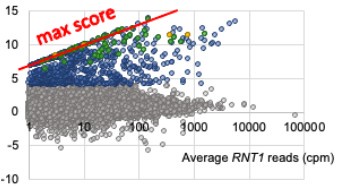
There are multiple ways to deal with this issue, and ours is not uncommon. DESeq2, suggested by the reviewer, uses a different method, which relies on the assumption that the dispersion of read counts for genes of any given expression strength is constant, and then uses that dispersion to “correct” the 0 read counts. While this is a valid way for differential gene expression when comparing similar RNAs, the underlying assumption that the dispersion of expression of all genes is similar for similar expression level is questionable for comparing, for example, mRNAs, snoRNAs, and snRNAs. Thus, we are not convinced that this is a better way to deal with 0 counts. Our analysis accepts that 0 might be the best estimate for the number of counts that are expected from rnt1∆ samples.
(3) The analysis in Figure S8 is insufficient to demonstrate that the four mRNAs depicted are significantly more abundant in rnt1Δ vs RNT1 cells - differences in coverage could simply be a result of different sequencing depth. Please use an appropriate method for estimating differential expression from RNA-Seq data (e.g., DESeq2).
Unfortunately, the previously published data we included as figure S8 (now figure S9) did not include replicates, and we agree that it does not rigorously show an effect. The reviewer suggests that we analyze the data by DESeq2, which requires replicates, and thus, cannot be done. Instead we have clarified this. If the reviewer is not satisfied with this, we are prepared to delete it.
-
-
www.biorxiv.org www.biorxiv.org
-
Author response:
The following is the authors’ response to the current reviews.
Reviewer #1 (Public review):
The authors present their new bioinformatic tool called TEKRABber, and use it to correlate expression between KRAB ZNFs and TEs across different brain tissues, and across species. While the aims of the authors are clear and there would be significant interest from other researchers in the field for a program that can do such correlative gene expression analysis across individual genomes and species, the presented approach and work display significant shortcomings. In the current state of the analysis pipeline, the biases and shortcomings mentioned below, for which I have seen no proof of that they are accounted for by the authors, are severely impacting the presented results and conclusions. It is therefore essential that the points below are addressed, involving significant changes in the TEKRABber progamm as well as the analysis pipeline, to prevent the identification of false positive and negative signals, that would severely affect the conclusions one can raise about the analysis.
Thank you very much for the insightful review of our manuscript. Since most of the comments on our revised version are not different from the comments on our first version, we repeated our previous answer, but wrote a new reply to the new concerns (please see the last two paragraphs).
We would also like to reiterate here that most of the critique of the reviewer concerns the performance of other tools and not TEKRABber presented in our manuscript. We consider it out of scope for this manuscript to improve other tools.
My main concerns are provided below:
One important shortcoming of the biocomputational approach is that most TEs are not actually expressed, and others (Alus) are not a proxy of the activity of the TE class at all. I will explain: While specific TE classes can act as (species-specific) promoters for genes (such as LTRs) or are expressed as TE derived transcripts (LINEs, SVAs), the majority of other older TE classes do not have such behavior and are either neutral to the genome or may have some enhancer activity (as mapped in the program they refer to 'TEffectR'. A big focus is on Alus, but Alus contribute to a transcriptome in a different way too: They often become part of transcripts due to alternative splicing. As such, the presence of Alu derived transcripts is not a proxy for the expression/activity of the Alu class, but rather a result of some Alus being part of gene transcripts (see also next point). Bottom line is that the TEKRABber software/approach is heavily prone to picking up both false positives (TEs being part of transcribed loci) and false negatives (TEs not producing any transcripts at all) , which has a big implication for how reads from TEs as done in this study should be interpreted: The TE expression used to correlate the KRAB ZNF expression is simply not representing the species-specific influences of TEs where the authors are after.
With the strategy as described, a lot of TE expression is misinterpreted: TEs can be part of gene-derived transcripts due to alternative splicing (often happens for Alus) or as a result of the TE being present in an inefficiently spliced out intron (happens a lot) which leads to TE-derived reads as a result of that TE being part of that intron, rather than that TE being actively expressed. As a result, the data as analysed is not reliably indicating the expression of TEs (as the authors intend too) and should be filtered for any reads that are coming from the above scenarios: These reads have nothing to do with KRAB ZNF control, and are not representing actively expressed TEs and therefore should be removed. Given that from my lab's experience in brain (and other) tissues, the proportion of RNA sequencing reads that are actually derived from active TEs is a stark minority compared to reads derived from TEs that happen to be in any of the many transcribed loci, applying this filtering is expected to have a huge impact on the results and conclusions of this study.
We sincerely thank the reviewer for highlighting the potential issues of false positives and negatives in TE quantification. The reviewer provided valuable examples of how different TE classes, such as Alus, LTRs, LINEs, and SVAs, exhibit distinct behaviors in the genome. To our knowledge, specific tools like ERVmap (Tokuyama et al., 2018), which annotates ERVs, and LtrDetector (Joseph et al., 2019), which uses k-mer distributions to quantify LTRs, could indeed enhance precision by treating specific TE classes individually. We acknowledge that such approaches may yield more accurate results and appreciate the suggestion.
In our study, we used TEtranscripts (Jin et al., 2015) prior to TEKRABber. TEtranscripts applies the Expectation Maximization (EM) algorithm to assign ambiguous reads as the following steps. Uniquely mapped reads are first assigned to genes, and reads overlapping genes and TEs are assigned to TEs only if they do not uniquely match an annotated gene. The remaining ambiguous reads are distributed based on EM iterations. While this approach may not be as specialized as the latest tools for specific TE classes, it provides a general overview of TE activity. TEtranscripts outputs subfamily-level TE expression data, which we used as input for TEKRABber to perform downstream analyses such as differential expression and correlation studies.
We understand the importance of adapting tools to specific research objectives, including focusing on particular TE classes. TEKRABber is designed not to refine TE quantification at the mapping stage but to flexibly handle outputs from various TE quantification tools. It accepts raw TE counts as input in the form of dataframes, enabling diverse analytical pipelines. We would also like to clarify that, since the input data is transcriptomic, our primary focus is on expressed TEs, rather than the effects of non-expressed TEs in the genome. In the revised version of our manuscript, we emphasize this distinction in the discussion and provide examples of how TEKRABber can integrate with other tools to enhance specificity and accuracy.
Another potential problem that I don't see addressed is that due to the high level of similarity of the many hundreds of KRAB ZNF genes in primates and the reads derived from them, and the inaccurate annotations of many KZNFs in non-human genomes, the expression data derived from RNA-seq datasets cannot be simply used to plot KZNF expression values, without significant work and manual curation to safeguard proper cross species ortholog-annotation: The work of Thomas and Schneider (2011) has studied this in great detail but genome-assemblies of non-human primates tend to be highly inaccurate in appointing the right ortholog of human ZNF genes. The problem becomes even bigger when RNA-sequencing reads are analyzed: RNA-sequencing reads from a human ZNF that emerged in great apes by duplication from an older parental gene (we have a decent number of those in the human genome) may be mapped to that older parental gene in Macaque genome: So, the expression of human-specific ZNF-B, that derived from the parental ZNF-A, is likely to be compared in their DESeq to the expression of ZNF-A in Macaque RNA-seq data. In other words, without a significant amount of manual curation, the DE-seq analysis is prone to lead to false comparisons which make the stategy and KRABber software approach described highly biased and unreliable.
There is no doubt that there are differences in expression and activity of KRAB-ZNFs and TEs repspectively that may have had important evolutionary consequences. However, because all of the network analyses in this paper rely on the analyses of RNA-seq data and the processing through the TE-KRABber software with the shortcomings and potential biases that I mentioned above, I need to emphasize that the results and conclusions are likely to be significantly different if the appropriate measures are taken to get more accurate and curated TE and KRAB ZNF expression data.
We thank the reviewer for raising the important issue of accurately annotating the expanded repertoire of KRAB-ZNFs in primates, particularly the challenges of cross-species orthology and potential biases in RNA-seq data analysis. Indeed, we have also addressed this challenge in some of our previous papers (Nowick et al., 2010, Nowick et al., 2011 and Jovanovic et al., 2021).
In the revised manuscript, we include more details about our two-step strategy to ensure accurate KRAB-ZNF ortholog assignments. First, we employed the Gene Order Conservation (GOC) score from Ensembl BioMart as a primary filter, selecting only one-to-one orthologs with a GOC score above 75% across primates. This threshold, recommended in Ensembl’s ortholog quality control guidelines, ensures high-confidence orthology relationships.(http://www.ensembl.org/info/genome/compara/Ortholog_qc_manual.html#goc).
Second, we incorporated data from Jovanovic et al. (2021), which independently validated KRAB-ZNF orthologs across 27 primate genomes. This additional layer of validation allowed us to refine our dataset, resulting in the identification of 337 orthologous KRAB-ZNFs for differential expression analysis (Figure S2).
We acknowledge that different annotation methods or criteria may for some genes yield variations in the identified orthologs. However, we believe that this combination provides a robust starting point for addressing the challenges raised, while we remain open to additional refinements in future analyses.
Finally, there are some minor but important notes I want to share:
The association with certain variations in ZNF genes with neurological disorders such as AD, as reported in the introduction is not entirely convincing without further functional support. Such associations could be merely happen by chance, given the high number of ZNF genes in the human genome and the high chance that variations in these loci happen associate with certatin disease associated traits. So using these associations as an argument that changes in TEs and KRAB ZNF networks are important for diseases like AD should be used with much more caution.
We fully acknowledge the concern that, given the large number of KRAB-ZNFs and their inherent variability, some associations with AD or other neurological disorders could occur by chance. This highlights the importance of additional functional studies to validate the causal role of KRAB-ZNF and TE interactions in disease contexts. While previous studies have indeed analyzed KRAB-ZNF and TE expression in human brain tissues, our study seeks to expand on this foundation by incorporating interspecies comparisons across primates. This approach enabled us to identify TE:KRAB-ZNF pairs that are uniquely present in healthy human brains, which may provide insights into their potential evolutionary significance and relevance to diseases like AD.
In addition to analyzing RNA-seq data (GSE127898 and syn5550404), we have cross-validated our findings using ChIP-exo data for 159 KRAB-ZNF proteins and their TE binding regions in humans (Imbeault et al., 2017). This allowed us to identify specific binding events between KRAB-ZNF and TE pairs, providing further support for the observed associations. We agree with the reviewer that additional experimental validations, such as functional studies, are critical to further establish the role of KRAB-ZNF and TE networks in AD. We hope that future research can build upon our findings to explore these associations in greater detail.
There is a number of papers where KRAB ZNF and TE expression are analysed in parallel in human brain tissues. So the novelty of that aspect of the presented study may be limited.
We agree with the reviewer that many studies have examined the expression levels of KRAB-ZNFs and TEs in developing human brain tissues (Farmiloe et al., 2020; Turelli et al., 2020; Playfoot et al., 2021, among others). However, the novelty of our study lies in comparing KRAB-ZNF and TE expression across primate species, as well as in adult human brain tissues from both control individuals and those with Alzheimer’s disease. To our knowledge, no previous study has analyzed these data in this context. We therefore believe that our results will be of interest to evolutionary biologists and neurobiologists focusing on Alzheimer’s disease.
Additional note after reviewing the revised version of the manuscript:
After reviewing the revised version of the manuscript, my criticism and concerns with this study are still evenly high and unchanged. To clarify, the revised version did not differ in essence from the original version; it seems that unfortunately, no efforts were taken to address the concerns raised on the original version of the manuscript, the results section as well as the discussion section are virtually unchanged.
We regret that this reviewer was not satisfied with our changes. In fact, many of the points raised by this reviewer are important, but concern weaknesses of other tools. In our opinion, validating other tools would be out of scope for this paper. We want to emphasize that TEKRABber is not a quantification tool for sequencing data, but a software for comparative analysis across species. We provided a detailed answer to the reviewer and readers can refer to that answer in the public review above for further information.
The following is the authors’ response to the original reviews.
Reviewer #1 (Public review):
The authors present their new bioinformatic tool called TEKRABber, and use it to correlate expression between KRAB ZNFs and TEs across different brain tissues, and across species. While the aims of the authors are clear and there would be significant interest from other researchers in the field for a program that can do such correlative gene expression analysis across individual genomes and species, the presented approach and work display significant shortcomings. In the current state of the analysis pipeline, the biases and shortcomings mentioned below, for which I have seen no proof that they are accounted for by the authors, are severely impacting the presented results and conclusions. It is therefore essential that the points below are addressed, involving significant changes in the TEKRABber program as well as the analysis pipeline, to prevent the identification of false positive and negative signals, that would severely affect the conclusions one can raise about the analysis.
Thank you very much for the insightful review of our manuscript.
My main concerns are provided below:
(1) One important shortcoming of the biocomputational approach is that most TEs are not actually expressed, and others (Alus) are not a proxy of the activity of the TE class at all. I will explain: While specific TE classes can act as (species-specific) promoters for genes (such as LTRs) or are expressed as TE derived transcripts (LINEs, SVAs), the majority of other older TE classes do not have such behavior and are either neutral to the genome or may have some enhancer activity (as mapped in the program they refer to 'TEffectR'. A big focus is on Alus, but Alus contribute to a transcriptome in a different way too: They often become part of transcripts due to alternative splicing. As such, the presence of Alu derived transcripts is not a proxy for the expression/activity of the Alu class, but rather a result of some Alus being part of gene transcripts (see also next point). The bottom line is that the TEKRABber software/approach is heavily prone to picking up both false positives (TEs being part of transcribed loci) and false negatives (TEs not producing any transcripts at all), which has a big implication for how reads from TEs as done in this study should be interpreted: The TE expression used to correlate the KRAB ZNF expression is simply not representing the species-specific influences of TEs where the authors are after.
With the strategy as described, a lot of TE expression is misinterpreted: TEs can be part of gene-derived transcripts due to alternative splicing (often happens for Alus) or as a result of the TE being present in an inefficiently spliced out intron (happens a lot) which leads to TE-derived reads as a result of that TE being part of that intron, rather than that TE being actively expressed. As a result, the data as analysed is not reliably indicating the expression of TEs (as the authors intend to) and should be filtered for any reads that are coming from the above scenarios: These reads have nothing to do with KRAB ZNF control, and are not representing actively expressed TEs and therefore should be removed. Given that from my lab's experience in the brain (and other) tissues, the proportion of RNA sequencing reads that are actually derived from active TEs is a stark minority compared to reads derived from TEs that happen to be in any of the many transcribed loci, applying this filtering is expected to have a huge impact on the results and conclusions of this study.
We sincerely thank the reviewer for highlighting the potential issues of false positives and negatives in TE quantification. The reviewer provided valuable examples of how different TE classes, such as Alus, LTRs, LINEs, and SVAs, exhibit distinct behaviors in the genome. To our knowledge, specific tools like ERVmap (Tokuyama et al., 2018), which annotates ERVs, and LtrDetector (Joseph et al., 2019), which uses k-mer distributions to quantify LTRs, could indeed enhance precision by treating specific TE classes individually. We acknowledge that such approaches may yield more accurate results and appreciate the suggestion.
In our study, we used TEtranscripts (Jin et al., 2015) prior to TEKRABber. TEtranscripts applies the Expectation Maximization (EM) algorithm to assign ambiguous reads as the following steps. Uniquely mapped reads are first assigned to genes, and reads overlapping genes and TEs are assigned to TEs only if they do not uniquely match an annotated gene. The remaining ambiguous reads are distributed based on EM iterations. While this approach may not be as specialized as the latest tools for specific TE classes, it provides a general overview of TE activity. TEtranscripts outputs subfamily-level TE expression data, which we used as input for TEKRABber to perform downstream analyses such as differential expression and correlation studies.
We understand the importance of adapting tools to specific research objectives, including focusing on particular TE classes. TEKRABber is designed not to refine TE quantification at the mapping stage but to flexibly handle outputs from various TE quantification tools. It accepts raw TE counts as input in the form of dataframes, enabling diverse analytical pipelines. We would also like to clarify that, since the input data is transcriptiomic, our primary focus is on expressed TEs, rather than the effects of non-expressed TEs in the genome. In the revised version of our manuscript, we emphasize this distinction in the discussion and provide examples of how TEKRABber can integrate with other tools to enhance specificity and accuracy.
(2) Another potential problem that I don't see addressed is that due to the high level of similarity of the many hundreds of KRAB ZNF genes in primates and the reads derived from them, and the inaccurate annotations of many KZNFs in non-human genomes, the expression data derived from RNA-seq datasets cannot be simply used to plot KZNF expression values, without significant work and manual curation to safeguard proper cross species ortholog-annotation: The work of Thomas and Schneider (2011) has studied this in great detail but genome-assemblies of non-human primates tend to be highly inaccurate in appointing the right ortholog of human ZNF genes. The problem becomes even bigger when RNA-sequencing reads are analyzed: RNA-sequencing reads from a human ZNF that emerged in great apes by duplication from an older parental gene (we have a decent number of those in the human genome) may be mapped to that older parental gene in Macaque genome: So, the expression of human-specific ZNF-B, that derived from the parental ZNF-A, is likely to be compared in their DESeq to the expression of ZNF-A in Macaque RNA-seq data. In other words, without a significant amount of manual curation, the DE-seq analysis is prone to lead to false comparisons which make the strategy and KRABber software approach described highly biased and unreliable.
There is no doubt that there are differences in expression and activity of KRAB-ZNFs and TEs respectively that may have had important evolutionary consequences. However, because all of the network analyses in this paper rely on the analyses of RNA-seq data and the processing through the TE-KRABber software with the shortcomings and potential biases that I mentioned above, I need to emphasize that the results and conclusions are likely to be significantly different if the appropriate measures are taken to get more accurate and curated TE and KRAB ZNF expression data.
We thank the reviewer for raising the important issue of accurately annotating the expanded repertoire of KRAB-ZNFs in primates, particularly the challenges of cross-species orthology and potential biases in RNA-seq data analysis. Indeed, we have also addressed this challenge in some of our previous papers (Nowick et al., 2010, Nowick et al., 2011 and Jovanovic et al., 2021).
In the revised manuscript, we include more details about our two-step strategy to ensure accurate KRAB-ZNF ortholog assignments. First, we employed the Gene Order Conservation (GOC) score from Ensembl BioMart as a primary filter, selecting only one-to-one orthologs with a GOC score above 75% across primates. This threshold, recommended in Ensembl’s ortholog quality control guidelines, ensures high-confidence orthology relationships. (http://www.ensembl.org/info/genome/compara/Ortholog_qc_manual.html#goc).
Second, we incorporated data from Jovanovic et al. (2021), which independently validated KRAB-ZNF orthologs across 27 primate genomes. This additional layer of validation allowed us to refine our dataset, resulting in the identification of 337 orthologous KRAB-ZNFs for differential expression analysis (Figure S2).
We acknowledge that different annotation methods or criteria may for some genes yield variations in the identified orthologs. However, we believe that this combination provides a robust starting point for addressing the challenges raised, while we remain open to additional refinements in future analyses.
(3) The association with certain variations in ZNF genes with neurological disorders such as AD, as reported in the introduction is not entirely convincing without further functional support. Such associations could merely happen by chance, given the high number of ZNF genes in the human genome and the high chance that variations in these loci happen to associate with certain disease-associated traits. So using these associations as an argument that changes in TEs and KRAB ZNF networks are important for diseases like AD should be used with much more caution.
There are a number of papers where KRAB ZNF and TE expression are analysed in parallel in human brain tissues. So the novelty of that aspect of the presented study may be limited.
We fully acknowledge the concern that, given the large number of KRAB-ZNFs and their inherent variability, some associations with AD or other neurological disorders could occur by chance. This highlights the importance of additional functional studies to validate the causal role of KRAB-ZNF and TE interactions in disease contexts. While previous studies have indeed analyzed KRAB-ZNF and TE expression in human brain tissues, our study seeks to expand on this foundation by incorporating interspecies comparisons across primates. This approach enabled us to identify TE:KRAB-ZNF pairs that are uniquely present in healthy human brains, which may provide insights into their potential evolutionary significance and relevance to diseases like AD.
In addition to analyzing RNA-seq data (GSE127898 and syn5550404), we have cross-validated our findings using ChIP-exo data for 159 KRAB-ZNF proteins and their TE binding regions in humans (Imbeault et al., 2017). This allowed us to identify specific binding events between KRAB-ZNF and TE pairs, providing further support for the observed associations. We agree with the reviewer that additional experimental validations, such as functional studies, are critical to further establish the role of KRAB-ZNF and TE networks in AD. We hope that future research can build upon our findings to explore these associations in greater detail.
Reviewer #1 (Recommendations for the authors):
It is essential before this work can be considered for publication, that the points above are addressed, involving significant changes in the TEKRABber program as well as the analysis pipeline, to prevent the identification of false positive and negative signals, that would severely affect the conclusions one can raise about the analysis.
We sincerely appreciate the reviewer’s insightful recommendations and constructive feedback. Each specific point has been carefully addressed in detail in the public reviews section above.
Reviewer #2 (Public review)
Summary:
The aim was to decipher the regulatory networks of KRAB-ZNFs and TEs that have changed during human brain evolution and in Alzheimer's disease.
Strengths:
This solid study presents a valuable analysis and successfully confirms previous assumptions, but also goes beyond the current state of the art.
Weaknesses:
The design of the analysis needs to be slightly modified and a more in-depth analysis of the positive correlation cases would be beneficial. Some of the conclusions need to be reinterpreted.
We sincerely thank the reviewer for the thoughtful summary, positive evaluation of our study, and constructive feedback. We appreciate the recognition of the strengths in our analysis and the valuable suggestions for improving its design and interpretation.
We would like to briefly comment on the suggested modifications to the design here and will provide a detailed point-by-point review later with our revised manuscript.
The reviewer recommended considering a more recent timepoint, such as less than 25 million years ago (mya), to define the "evolutionary young group" of KRAB-ZNF genes and TEs when discussing the arms-race theory. This is indeed a valuable perspective, as the TE repressing functions by KRAB-ZNF proteins may have evolved more recently than the split between Old World Monkeys (OWM) and New World Monkeys (NWM) at 44.2 mya we used.
Our rationale for selecting 44.2 mya is based on certain primate-specific TEs such as the Alu subfamilies, which emerged after the rise of Simiiformes and have been used in phylogenetic studies (Xing et al., 2007 and Williams et al., 2010). This timeframe allowed us to investigate the potential co-evolution of KRAB-ZNFs and TEs in species that emerged after the OWM-NWM split (e.g., humans, chimpanzees, bonobos, and macaques used for this study). However, focusing only on KRAB-ZNFs and TEs younger than 25 million years would limit the analysis to just 9 KRAB-ZNFs and 92 TEs expressed in our datasets. While we will not conduct a reanalysis using this more recent timepoint, we will integrate the recommendation into the discussion section of the revised manuscript.
Furthermore, we greatly appreciate the reviewer's detailed insights and suggestions for refining specific descriptions and interpretations in our manuscript. We will address these points in the revised version to ensure the content is presented with greater precision and clarity.
Once again, we thank both reviewers for their valuable feedback, which provides significant input for strengthening our study.
Reviewer #2 (Recommendations for the authors):
We thank the reviewer for the very insightful comments, which helped a lot in our interpretation and discussion of our results and in improving some of our statements.
The present study seeks to uncover how the repression of transposable elements (TEs) by rapidly evolving KRAB-ZNF genes, which are known for their role in TE suppression, may influence human brain evolution and contribute to Alzheimer's disease (AD). Utilizing their previously developed tool, TEKRABber, the researchers analyze transcriptome datasets from the brains of four species of Old World Monkeys (OWM) alongside samples from healthy human individuals and AD patients.
Through bipartite network analysis, they identify KRAB-ZNF/Alu-TE interactions as the most negatively correlated in the network, highlighting the repression of Alu elements by KRAB-ZNF proteins. In AD patient samples, they observe a reduction in a subnetwork comprising 21 interactions within an Alu TE module. These findings are consistent with earlier evidence that: (1) KRAB-ZNFs are involved in suppressing evolutionarily young Alu TEs; and (2) specific Alu elements have been reported to be deregulated in AD. The study also validates previous experimental ChIP-exo data on KRAB-ZNF proteins obtained in a different cell type (Imbeault et al., 2017).
As a novely, the study identifies a human-specific amino acid variation in ZNF528, which directly contacts DNA nucleotides, showing signs of positive selection in humans and several human-specific TE interactions.
Interestingly, in addition to the negative links, the researchers observed predominantly positive connections with other TEs, suggesting that while their approach is consistent with some previous observations, the authors conclude that it provides limited support for the 'genetic arms race' hypothesis.
The reviewer is a specialist in TE and evolutionary research.
Major issues:
The study demonstrates the usefulness of the TEKRABber tool, which can support and successfully validate previous observations. However, there are several misconceptions and problems with the interpretation of the results.
KRAB-ZNF proteins in repressing TEs in vertebrates In the Abstract: "In vertebrates, some KRAB-ZNF proteins repress TEs, offering genomic protection."
Although some KRAB-ZNF proteins exist in vertebrates, their TE-suppression role is not as prominent or specialized as it is in mammals, where it serves as a key defense mechanism against the mobilization of TEs.
We appreciate the reviewer’s clarification regarding the role of KRAB-ZNF proteins in vertebrates. To improve accuracy and precision, we have revised the wording to specify that this mechanism is primarily observed in mammals rather than vertebrates.
The definition of young and old
The study considers the evolutionary age of young ({less than or equal to} 44.2 mya) and old(> 44.2 mya). This is the time of the Old World Monkey (OWM) and New World Monkey (NWM) split. Importantly, however, the KRAB-ZNF / KAP1 suppression system primarily suppresses evolutionarily younger TEs (< 25 MY old). These TEs are relatively new additions to the genome, i.e. they are specific to certain lineages (such as primates or hominins) and are more likely to be actively transcribed (and recognized as foreign by innate immunity) or have residual activity upon transposition. Examples include certain subfamilies of LINE-1, Alu (Y, S, less effective for J), SVA and younger human endogenous retroviruses (HERVs) such as HERV-K. The KRAB-ZNF / KAP1 system therefore focuses primarily on TEs that have evolved more recently in primates, in the last few million years (within the last 25 million years). Older TEs are controlled by broader epigenetic mechanisms such as DNA methylation, histone modifications, etc. Therefore, the age ({less than or equal to} 44.2 mya) is not suitable to define it as young.
In this context, the specific TEs of the Simiiformes cannot be considered as 'recently evolved' (in the Abstract). The Simiiformes contain both OWM and NWM. Notably, the study includes four species, all of which belong to the OWMs.
The 'genetic arms race' theory
Unfortunately, the problematic definition of young and old could also explain why the authors conclude that their data only weakly support the 'genetic arms race' hypothesis.
The KRAB-ZNF proteins evolve rapidly, similar to TEs, which raises the 'genetic arms race' hypothesis. This hypothesis refers to the constant evolutionary struggle between organisms and TEs. TEs constantly evolve to overcome host defences, while host genomes develop mechanisms to suppress these potentially harmful elements. Indeed, in mammals, an important example is the KRAB-ZNF/TE interaction. The KRAB-ZNF proteins rapidly evolve to target specific TEs, creating a 'genetic arms race' in which each side - TEs and the KRAB-ZNF/KAP1 (alias TRIM28) repressor complex - drives the evolution of the other in response to adaptive pressure. Importantly, the 'genetic arms race' hypothesis describes the evolutionary process that occurs between TE and host when the TE is deleterious. Again, this includes the young TEs (< 25 MY old) with residual transposition activity or those that actively transcribed and exacerbate cellular stress and inflammatory responses. Approximately 25 million years ago, the superfamilies Hominoidea (apes) and Cercopithecoidea (Old World monkeys, I.e. macaque) split.
Just to clarify, our initial study aim was to examine whether TEs exhibit any evolutionary relationships with KRAB-ZNFs across the four studied species (human, chimpanzee, bonobo, and macaque). For investigating the arms-race hypothesis, we really appreciate the reviewer suggesting a more recent time point, such as less than 25 million years ago (mya), to define the "evolutionary young group" of TEs and KRAB-ZNF genes. This is indeed a valuable recommendation, as 25 mya marks the emergence of Hominoidea (Figure 2C in the manuscript), making it a meaningful reference point for studying recently evolved KRAB-ZNFs and TEs. However, restricting the analysis to elements younger than 25 mya would reduce the dataset to only 9 KRAB-ZNFs and 92 TEs. Nevertheless, we provide here our results for those elements in Table S7:
We observed that among the correlations in the < 25 mya subset, negative correlations (7) outnumbered positive ones (2). However, these correlations were derived from only 3 out of 9 KRAB-ZNFs and 9 out of 92 TE subfamilies. Therefore, based on our data, while the < 25 mya group shows a higher proportion of negative correlations, the sample size is too limited to derive networks or draw robust conclusions in our analysis, especially when compared to our original evolutionary age threshold of 44.2 mya. For this reason, we chose not to reanalyze the data but rather to acknowledge that our current definition of “young” may not be optimal for testing the arms-race model in humans. While previous studies (Jacobs et al., 2014; Bruno et al., 2019; Zuo et al., 2023) have explored relevant KRAB-ZNF and TE interactions, our review of the KRAB-ZNFs and TEs highlighted in those works suggests that a specific focus on elements <25 mya has not been a primary emphasis.
"our findings only weakly support the arms-race hypothesis. Firstly, we noted that young TEs exhibit lower expression levels than old TEs (Figure 2D and 5B), which might not be expected if they had recently escaped repression". - This is a misinterpretation. These old TEs are no longer harmful. This is not the case of the 'genetic arms race'.
We sincerely appreciate the reviewer’s comments, which have helped us refine our interpretation to prevent potential misunderstandings. Our initial expectation, based on the arms-race hypothesis, was that young TEs would exhibit higher expression levels due to a recent escape from repression, while young KRAB-ZNFs would show increased expression as a counter-adaptive response. However, our findings indicate that both young TEs and young KRAB-ZNFs exhibit lower expression levels. This observation does not align with the classical arms-race model, which typically predicts an ongoing cycle of adaptive upregulation. We rephrase the sentences in our discussion to hopefully make our idea more clear. In addition, we added the notion that older TEs might not be harmful anymore, which we agree with.
"Additionally, some young TEs were also negatively correlated with old KRAB-ZNF genes, leading to weak assortativity regarding age inference, which would also not be in line with the arms-race idea."
This is not a contradiction, as an old KRAB-ZNF gene could be 'reactivated' to protect against young TEs. (It might be cheaper for the host than developing a brand new KRAB-ZNF gene.
We agree with the reviewer's point that older KRAB-ZNFs may be reactivated to suppress young TEs, potentially as a more cost-effective evolutionary strategy than the emergence of entirely new KRAB-ZNFs. We have incorporated this perspective into the revised manuscript to provide a more detailed discussion of our findings.
TEs remain active
In the abstract: "Notably, KRAB-ZNF genes evolve rapidly and exhibit diverse expression patterns in primate brains, where TEs remain active."
This is not precise. TEs are not generally remain active in the brain. It is only the autonomous LINE-1 (young) and non-autonomous Alu (young) and SVA (young) elements that can be mobilized by LINE-1. In addition, the evolutionary young HERV-K is recognized as foreign and alerts the innate immune system (DOI: 10.1172/jci.insight.131093 ) and is a target of the KRAB-ZNF/KAP1 suppression system.
In the abstract: "Evidence indicates that transposable elements (TEs) can contribute to the evolution of new traits, despite often being considered deleterious."
Oversimplification: The harmful and repurposed TEs are washed together.
We appreciate the reviewer’s detailed suggestions for improving the precision of our abstract. While we previously mentioned LINE-1 and Alu elements in the introduction, we now explicitly specify in the abstract that only certain TE subfamilies, such as autonomous LINE-1 and non-autonomous Alu and SVA elements, remain active in the primate brain. Additionally, we have refined the phrasing regarding the role of TEs in evolution to clearly distinguish between their deleterious effects and their potential for functional repurposing. These clarifications have been incorporated into the revised abstract to ensure greater accuracy and nuance.
Positive links
"The high number of positive correlations might be surprising, given that KRAB-ZNFs are considered to repress TEs."
Based on the above, it is not surprising that negative associations are only found with young (< 25 my) TEs. In fact, the relationship between old KRAB-ZNF proteins and old (non-damaging) TEs could be neutral/positive. The case of ZNF528 could be a valuable example of this.
We thank the reviewer for providing this plausible interpretation and added it to the manuscript.
"276 TE:KRAB-ZNF with positive correlations in humans were negatively correlated in bonobos" It would be important to characterise the positive correlations in more detail. Could it be that the old KRAB-ZNF proteins lost their ability to recruit KAP1/TRIM28? Demonstrate it.
The strategy of developing sequence-specific DNA recognition domains that can specifically recognise TEs is expensive for the host. Recent studies suggest that when the TE is no longer harmful, these proteins/connections can be occasionally repurposed. The repurposed function would probably differ from the original suppressive function.
In my opinion, the TEKRABber tool could be useful in identifying co-option events:
We appreciate the reviewer’s suggestion regarding the characterization of positive correlations. While it is possible that some old KRAB-ZNF proteins have lost their ability to recruit KAP1/TRIM28, we cannot conclude this definitively for all cases. To address this, we examined ChIP-exo data from Imbeault et al. (2017) (Accession: GSE78099) and analyzed the overlap of binding sites between KRAB-ZNFs, KAP1/TRIM28, and RepeatMasker-annotated TEs. Our results indicate that some old KRAB-ZNFs still exhibit binding overlap with KAP1 at TE regions, suggesting that their repressive function may be at least partially retained (Author response image 1).
Author response image 1.<br /> Overlap of KAP1, Zinc finger proteins, and RepeatMasker annotation. Here we detect the overlap of ChIP-exo binding events using KAP1/TRIM28, with KRAB-ZNF genes (one at a time) and RepeatMasker annotation. (115 old and 58 young KRAB-ZNFs, Mann-Whitney, p<0.01).<br />
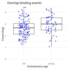
Minor
"Lead poisoning causes lead ions to compete with zinc ions in zinc finger proteins, affecting proteins such as DNMT1, which are related to the progression of AD (Ordemann and Austin 2016)."
Not precise: While DNMT1 does contain zinc-binding domains, it is not categorized as a zinc finger protein.
We appreciate the reviewer’s insight regarding the classification of DNMT1. After careful consideration, we have removed this sentence from the introduction to maintain focus on KRAB zinc finger proteins.
Definition of TEs
"There were 324 KRAB-ZNFs and 895 TEs expressed in Primate Brain Data." Define it more precisely. It is not clear, what the authors mean by TEs: Are these TE families, subfamilies? Provide information on copy numbers of each in the analysed four species.
We appreciate the reviewer’s suggestion to clarify our definition of TEs. To improve precision, we have specified that the analysis was conducted at the subfamily level. Additionally, we have provided the copy numbers of TEs for the four analyzed species in Table S4.
Occupancy of TEs in the genome
"TEs comprise (i) one third to one half of the mammalian genome and are (ii) not randomly distributed..."
(i) The most accepted number is 45%. However, some more recent reports estimate over 50%, thus the one third is an underestimation.
(ii) Not randomly distributed among the mammalian species?
(i) We thank the reviewer for pointing out that our statement about the abundance of TEs was outdated. We have updated the estimate to reflect that TEs can occupy more than half of the genome, based on recent publications.
(ii) We acknowledge the reviewer’s concern regarding the distribution of TEs. Although TEs are interspersed throughout the genome, their insertion sites are not entirely random, as they tend to exhibit preferences for certain genomic regions. To clarify this, we have revised the wording in the paragraph accordingly.
We would like to express our sincere gratitude to both reviewers for their insightful feedback, which has been instrumental in enhancing the quality of our study.
-
-
www.biorxiv.org www.biorxiv.org
-
Author response:
The following is the authors’ response to the original reviews.
Reviewer #1 (Public review):
Summary:
The authors propose a new technique which they name "Multi-gradient Permutation Survival Analysis (MEMORY)" that they use to identify "Genes Steadily Associated with Prognosis (GEARs)" using RNA-seq data from the TCGA database. The contribution of this method is one of the key stated aims of the paper. The vast majority of the paper focuses on various downstream analyses that make use of the specific GEARs identified by MEMORY to derive biological insights, with a particular focus on lung adenocarcinoma (LUAD) and breast invasive carcinoma (BRCA) which are stated to be representative of other cancers and are observed to have enriched mitosis and immune signatures, respectively. Through the lens of these cancers, these signatures are the focus of significant investigation in the paper.
Strengths:
The approach for MEMORY is well-defined and clearly presented, albeit briefly. This affords statisticians and bioinformaticians the ability to effectively scrutinize the proposed methodology and may lead to further advancements in this field.
The scientific aspects of the paper (e.g., the results based on the use of MEMORY and the downstream bioinformatics workflows) are conveyed effectively and in a way that is digestible to an individual who is not deeply steeped in the cancer biology field.
Weaknesses:
I was surprised that comparatively little of the paper is devoted to the justification of MEMORY (i.e., the authors' method) for the identification of genes that are important broadly for the understanding of cancer. The authors' approach is explained in the methods section of the paper, but no rationale is given for why certain aspects of the method are defined as they are. Moreover, no comparison or reference is made to any other methods that have been developed for similar purposes and no results are shown to illustrate the robustness of the proposed method (e.g., is it sensitive to subtle changes in how it is implemented).
For example, in the first part of the MEMORY algorithm, gene expression values are dichotomized at the sample median and a log-rank test is performed. This would seemingly result in an unnecessary loss of information for detecting an association between gene expression and survival. Moreover, while dichotomizing at the median is optimal from an information theory perspective (i.e., it creates equally sized groups), there is no reason to believe that median-dichotomization is correct vis-à-vis the relationship between gene expression and survival. If a gene really matters and expression only differentiates survival more towards the tail of the empirical gene expression distribution, median-dichotomization could dramatically lower the power to detect group-wise differences.
Thanks for these valuable comments!! We understand the reviewer’s concern regarding the potential loss of information caused by median-based dichotomization. In this study, we adopted the median as the cut-off value to stratify gene expression levels primarily for the purpose of data balancing and computational simplicity. This approach ensures approximately equal group sizes, which is particularly beneficial in the context of limited sample sizes and repeated sampling. While we acknowledge that this method may discard certain expression nuances, it remains a widely used strategy in survival analysis. To further evaluate and potentially enhance sensitivity, alternative strategies such as percentile-based cutoffs or survival models using continuous expression values (e.g., Cox regression) may be explored in future optimization of the MEMORY pipeline. Nevertheless, we believe that this dichotomization approach offers a straightforward and effective solution for the initial screening of survival-associated genes. We have now included this explanation in the revised manuscript (Lines 391–393).
Specifically, the authors' rationale for translating the Significant Probability Matrix into a set of GEARs warrants some discussion in the paper. If I understand correctly, for each cancer the authors propose to search for the smallest sample size (i.e., the smallest value of k_{j}) were there is at least one gene with a survival analysis p-value <0.05 for each of the 1000 sampled datasets. I base my understanding on the statement "We defined the sampling size k_{j} reached saturation when the max value of column j was equal to 1 in a significant-probability matrix. The least value of k_{j} was selected". Then, any gene with a p-value <0.05 in 80% of the 1000 sampled datasets would be called a GEAR for that cancer. The 80% value here seems arbitrary but that is a minor point. I acknowledge that something must be chosen. More importantly, do the authors believe this logic will work effectively in general? Presumably, the gene with the largest effect for a cancer will define the value of K_{j}, and, if the effect is large, this may result in other genes with smaller effects not being selected for that cancer by virtue of the 80% threshold. One could imagine that a gene that has a small-tomoderate effect consistently across many cancers may not show up as a gear broadly if there are genes with more substantive effects for most of the cancers investigated. I am taking the term "Steadily Associated" very literally here as I've constructed a hypothetical where the association is consistent across cancers but not extremely strong. If by "Steadily Associated" the authors really mean "Relatively Large Association", my argument would fall apart but then the definition of a GEAR would perhaps be suboptimal. In this latter case, the proposed approach seems like an indirect way to ensure there is a reasonable effect size for a gene's expression on survival.
Thank you for the comment and we apologize for the confusion! 𝐴<sub>𝑖𝑗</sub> refers to the value of gene i under gradient j in the significant-probability matrix, primarily used to quantify the statistical probability of association with patient survival for ranking purposes. We believe that GEARs are among the top-ranked genes, but there is no established metric to define the optimal threshold. An 80% threshold is previously employed as an empirical standard in studies related to survival estimates [1]. In addition, we acknowledge that the determination of the saturation point 𝑘<sub>𝑗</sub> is influenced by the earliest point at which any gene achieves consistent significance across 1000 permutations. We recognize that this may lead to the under representation of genes with moderate but consistent effects, especially in the presence of highly significant genes that dominate the statistical landscape. We therefore empirically used 𝐴<sub>𝑖𝑗</sub> > 0.8 the threshold to distinguish between GEARs and non-GEARs. Of course, this parameter variation may indeed result in the loss of some GEARs or the inclusion of non-GEARs. We also agree that future studies could investigate alternative metrics and more refined thresholds to improve the application of GEARs.
Regarding the term ‘Steadily Associated’, we define GEARs based on statistical robustness across subsampled survival analyses within individual cancer types, rather than cross-cancer consistency or pan-cancer moderate effects. Therefore, our operational definition of “steadiness” emphasizes within-cancer reproducibility across sampling gradients, which does not necessarily exclude high-effect-size genes. Nonetheless, we agree that future extensions of MEMORY could incorporate cross-cancer consistency metrics to capture genes with smaller but reproducible pan-cancer effects.
The paper contains numerous post-hoc hypothesis tests, statements regarding detected associations and correlations, and statements regarding statistically significant findings based on analyses that would naturally only be conducted in light of positive results from analyses upstream in the overall workflow. Due to the number of statistical tests performed and the fact that the tests are sometimes performed using data-driven subgroups (e.g., the mitosis subgroups), it is highly likely that some of the findings in the work will not be replicable. Of course, this is exploratory science, and is to be expected that some findings won't replicate (the authors even call for further research into key findings). Nonetheless, I would encourage the authors to focus on the quantification of evidence regarding associations or claims (i.e., presenting effect estimates and uncertainty intervals), but to avoid the use of the term statistical significance owing to there being no clear plan to control type I error rates in any systematic way across the diverse analyses there were performed.
Thank you for the comment! We agree that rigorous control of type-I error is essential once a definitive list of prognostic genes is declared. The current implementation of MEMORY, however, is deliberately positioned as an exploratory screening tool: each gene is evaluated across 10 sampling gradients and 1,000 resamples per gradient, and the only quantity carried forward is its reproducibility probability (𝐴<sub>𝑖𝑗</sub>).
Because these probabilities are derived from aggregate “votes” rather than single-pass P-values, the influence of any one unadjusted test is inherently diluted. In another words, whether or not a per-iteration BH adjustment is applied does not materially affect the ranking of genes by reproducibility, which is the key output at this stage. However, we also recognize that a clinically actionable GEARs catalogue will require extensive, large-scale multiple-testing adjustments. Accordingly, future versions of MEMORY will embed a dedicated false-positive control framework tailored to the final GEARs list before any translational application. We have added this point in the ‘Discussion’ in the revised manuscript (Lines 350-359).
A prespecified analysis plan with hypotheses to be tested (to the extent this was already produced) and a document that defines the complete scope of the scientific endeavor (beyond that which is included in the paper) would strengthen the contribution by providing further context on the totality of the substantial work that has been done. For example, the focus on LUAD and BRCA due to their representativeness could be supplemented by additional information on other cancers that may have been investigated similarly but where results were not presented due to lack of space.
We thank the reviewer for requesting greater clarity on the analytic workflow. The MEMORY pipeline was fully specified before any results were examined and is described in ‘Methods’ (Lines 386–407). By contrast, the pathway-enrichment and downstream network/mutation analyses were deliberately exploratory: their exact content necessarily depended on which functional categories emerged from the unbiased GEAR screen.
Our screen revealed a pronounced enrichment of mitotic signatures in LUAD and immune signatures in BRCA.
We then chose these two cancer types for deeper “case-study” analysis because they contained the largest sample sizes among all cancers showing mitotic- or immune-dominated GEAR profiles, and provided the greatest statistical power for follow-up investigations. We have added this explanation into the revised manuscript (Line 163, 219-220).
Reviewer #2 (Public review):
Summary:
The authors are trying to come up with a list of genes (GEAR genes) that are consistently associated with cancer patient survival based on TCGA database. A method named "Multi-gradient Permutation Survival Analysis" was created based on bootstrapping and gradually increasing the sample size of the analysis. Only the genes with consistent performance in this analysis process are chosen as potential candidates for further analyses.
Strengths:
The authors describe in detail their proposed method and the list of the chosen genes from the analysis. The scientific meaning and potential values of their findings are discussed in the context of published results in this field.
Weaknesses:
Some steps of the proposed method (especially the definition of survival analysis similarity (SAS) need further clarification or details since it would be difficult if anyone tries to reproduce the results. In addition, the multiplicity (a large number of p-values are generated) needs to be discussed and/or the potential inflation of false findings needs to be part of the manuscript.
Thank you for the reviewer’s insightful comments. Accordingly, in the revised manuscript, we have provided a more detailed explanation of the definition and calculation of Survival-Analysis Similarity (SAS) to ensure methodological clarity and reproducibility (Lines 411-428); and the full code is now publicly available on GitHub (https://github.com/XinleiCai/MEMORY). We have also expanded the ‘Discussion’ to clarify our position on false-positive control: future releases of MEMORY will incorporate a dedicated framework to control false discoveries in the final GEARs catalogue, where itself will be subjected to rigorous, large-scale multiple-testing adjustment.
If the authors can improve the clarity of the proposed method and there is no major mistake there, the proposed approach can be applied to other diseases (assuming TCGA type of data is available for them) to identify potential gene lists, based on which drug screening can be performed to identify potential target for development.
Thank you for the suggestion. All source code has now been made publicly available on GitHub for reference and reuse. We agree that the GEAR lists produced by MEMORY hold considerable promise for drugscreening and target-validation efforts, and the framework could be applied to any disease with TCGA-type data. Of course, we also notice that the current GEAR catalogue should first undergo rigorous, large-scale multipletesting correction to further improve its precision before broader deployment.
Reviewer #3 (Public review):
Summary:
The authors describe a valuable method to find gene sets that may correlate with a patient's survival. This method employs iterative tests of significance across randomised samples with a range of proportions of the original dataset. Those genes that show significance across a range of samples are chosen. Based on these gene sets, hub genes are determined from similarity scores.
Strengths:
MEMORY allows them to assess the correlation between a gene and patient prognosis using any available transcriptomic dataset. They present several follow-on analyses and compare the gene sets found to previous studies.
Weaknesses:
Unfortunately, the authors have not included sufficient details for others to reproduce this work or use the MEMORY algorithm to find future gene sets, nor to take the gene findings presented forward to be validated or used for future hypotheses.
Thank you for the reviewer’s comments! We apologize for the inconvenience and the lack of details.
Followed the reviewer’s valuable suggestion, we have now made all source code and relevant scripts publicly available on GitHub to ensure full reproducibility and facilitate future use of the MEMORY algorithm for gene discovery and hypothesis generation.
Reviewer #4 (Public review):
The authors apply what I gather is a novel methodology titled "Multi-gradient Permutation Survival Analysis" to identify genes that are robustly associated with prognosis ("GEARs") using tumour expression data from 15 cancer types available in the TCGA. The resulting lists of GEARs are then interrogated for biological insights using a range of techniques including connectivity and gene enrichment analysis.
I reviewed this paper primarily from a statistical perspective. Evidently, an impressive amount of work has been conducted, and concisely summarised, and great effort has been undertaken to add layers of insight to the findings. I am no stranger to what an undertaking this would have been. My primary concern, however, is that the novel statistical procedure proposed, and applied to identify the gene lists, as far as I can tell offers no statistical error control or quantification. Consequently, we have no sense of what proportion of the highlighted GEAR genes and networks are likely to just be noise.
Major comments:
(1) The main methodology used to identify the GEAR genes, "Multi-gradient Permutation Survival Analysis" does not formally account for multiple testing and offers no formal error control. Meaning we are left with no understanding of what the family-wise (aka type 1) error rate is among the GEAR lists, nor the false discovery rate. I would generally recommend against the use of any feature selection methodology that does not provide some form of error quantification and/or control because otherwise we do not know if we are encouraging our colleagues and/or readers to put resources into lists of genes that contain more noise than not. There are numerous statistical techniques available these days that offer error control, including for lists of p-values from arbitrary sets of tests (see expansion on this and some review references below).
Thank you for your thoughtful and important comment! We fully agree that controlling type I error is critical when identifying gene sets for downstream interpretation or validation. As an exploratory study, our primary aim was to define and screen for GEARs by using the MEMORY framework; however, we acknowledge that the current implementation of MEMORY does not include a formal procedure for error control. Given that MEMORY relies on repeated sampling and counts the frequency of statistically significant p-values, applying standard p-value–based multiple-testing corrections at the individual test level would not meaningfully reduce the false-positive rate in this framework.
We believe that error control should instead be applied at the level of the final GEAR catalogue. However, we also recognize that conventional correction methods are not directly applicable. In future versions of MEMORY, we plan to incorporate a dedicated and statistically appropriate false-positive control module tailored specifically to the aggregated outputs of the pipeline. We have clarified this point explicitly in the revised manuscript. (Lines 350-359)
(2) Similarly, no formal significance measure was used to determine which of the strongest "SAS" connections to include as edges in the "Core Survival Network".
We agree that the edges in the Core Survival Network (CSN) were selected based on the top-ranked SAS values rather than formal statistical thresholds. This was a deliberate design choice, as the CSN was intended as a heuristic similarity network to prioritize genes for downstream molecular classification and biological exploration, not for formal inference. To address potential concerns, we have clarified this intent in the revised manuscript, and we now explicitly state that the network construction was based on empirical ranking rather than statistical significance (Lines 422-425).
(3) There is, as far as I could tell, no validation of any identified gene lists using an independent dataset external to the presently analysed TCGA data.
Thank you for the comment. We acknowledge that no independent external dataset was used in the present study to validate the GEARs lists. However, the primary aim of this work was to systematically identify and characterize genes with robust prognostic associations across cancer types using the MEMORY framework. To assess the biological relevance of the resulting GEARs, we conducted extensive downstream analyses including functional enrichment, mutation profiling, immune infiltration comparison, and drug-response correlation. These analyses were performed across multiple cancer types and further supported by a wide range of published literature.
We believe that this combination of functional characterization and literature validation provides strong initial support for the robustness and relevance of the GEARs lists. Nonetheless, we agree that validation in independent datasets is an important next step, and we plan to carry this out in future work to further strengthen the clinical application of MEMORY.
(4) There are quite a few places in the methods section where descriptions were not clear (e.g. elements of matrices referred to without defining what the columns and rows are), and I think it would be quite challenging to re-produce some aspects of the procedures as currently described (more detailed notes below).
We apologize for the confusion. In the revised manuscript, we have provided a clearer and more detailed description of the computational workflow of MEMORY to improve clarity and reproducibility.
(5) There is a general lack of statistical inference offered. For example, throughout the gene enrichment section of the results, I never saw it stated whether the pathways highlighted are enriched to a significant degree or not.
We apologize for not clearly stating this information in the original manuscript. In the revised manuscript, we have updated the figure legend to explicitly report the statistical significance of the enriched pathways (Line 870, 877, 879-880).
Reviewer #1 (Recommendations for the authors):
Overall, the paper reads well but there are numerous small grammatical errors that at times cost me non-trivial amounts of time to understand the authors' key messages.
We apologize for the grammatical errors that hindered clarity. In response, we have thoroughly revised the manuscript for grammar, spelling, and overall language quality.
Reviewer #2 (Recommendations for the authors):
Major comments:
(1) Line 427: survival analysis similarity (SAS) definition. Any reference on this definition and why it is defined this way? Can the SAS value be negative? Based on line 429 definition, if A and B are exactly the same, SAS ~ 1; completely opposite, SAS =0; otherwise, SAS could be any value, positive or negative. So it is hard to tell what SAS is measuring. It is important to make sure SAS can measure the similarity in a systematic and consistent way since it is used as input in the following network analysis.
We apologize for the confusion caused by the ambiguity in the original SAS formula. The SAS metric was inspired by the Jaccard index, but we modified the denominator to increase contrast between gene pairs. Specifically, the numerator counts the number of permutations in which both genes are simultaneously significant (i.e., both equal to 1), while the denominator is the sum of the total number of significant events for each gene minus twice the shared significant count. An additional +1 term was included in the denominator to avoid division by zero. This formulation ensures that SAS is always non-negative and bounded between 0 and 1, with higher values indicating greater similarity. We have clarified this definition and updated the formula in the revised manuscript (Lines 405-425).
(2) For the method with high dimensional data, multiplicity adjustment needs to be discussed, but it is missing in the manuscript. A 5% p-value cutoff was used across the paper, which seems to be too liberal in this type of analysis. The suggestion is to either use a lower cutoff value or use False Discovery Rate (FDR) control methods for such adjustment. This will reduce the length of the gene list and may help with a more focused discussion.
We appreciate the reviewer’s suggestion regarding multiplicity. MEMORY is intentionally positioned as an exploratory screen: each gene is tested across 10 sampling gradients and 1,000 resamples, and only its reproducibility probability (𝐴<sub>𝑖𝑗</sub>) is retained. Because this metric is an aggregate of 1,000 “votes” the influence of any single unadjusted P-value is already strongly diluted; adding a per-iteration BH/FDR step therefore has negligible impact on the reproducibility ranking that drives all downstream analyses.
That said, we recognize that a clinically actionable GEARs catalogue must undergo formal, large-scale multipletesting correction. Future releases of MEMORY will incorporate an error control module applied to the consolidated GEAR list before any translational use. We have now added a statement to this effect in the revised manuscript (Lines 350-359).
(3) To allow reproducibility from others, please include as many details as possible (software, parameters, modules etc.) for the analyses performed in different steps.
All source codes are now publically available on GitHub. We have also added the GitHub address in the section Online Content.
Minor comments or queries:
(4) The manuscript needs to be polished to fix grammar, incomplete sentences, and missing figures.
Thank you for the suggestion. We have thoroughly proofread the manuscript to correct grammar, complete any unfinished sentences, and restore or renumber all missing figure panels. All figures are now properly referenced in the text.
(5) Line 131: "survival probability of certain genes" seems to be miss-leading. Are you talking about its probability of associating with survival (or prognosis)?
Sorry for the oversight. What we mean is the probability that a gene is found to be significantly associated with survival across the 1,000 resamples. We have revised the statement to “significant probability of certain genes” (Line 102).
(6) Lines 132, 133: "remained consistent": the score just needs to stay > 0.8 as the sample increases, or the score needs to be monotonously non-decreasing?
We mean the score stay above 0.8. We understand “remained consistent” is confusing and now revised it to “remained above 0.8”.
(7) Lines 168-170 how can supplementary figure 5A-K show "a certain degree of correlation with cancer stages"?
Sorry for the confusion! We have now revised Supplementary Figure 5A–K to support the visual impression with formal statistics. For each cancer type, we built a contingency table of AJCC stage (I–IV) versus hub-gene subgroup (Low, Mid, High) and applied Pearson’s 𝑥<sup>2</sup> test (Monte-Carlo approximation, 10⁵ replicates when any expected cell count < 5). The 𝑥<sup>2</sup> statistic and p-value are printed beneath every panel; eight of the eleven cancers show a significant association (p-value < 0.05), while LUSC, THCA and PAAD do not.We have replaced the vague phrase “a certain degree of correlation” with this explicit statistical statement in the revised manuscript (Lines 141-143).
(8) Lines 172-174: since the hub genes are a subset of GEAR genes through CSN construction, it is not a surprise of the consistency. any explanation about PAAD that is shown only in GOEA with GEARs but not with hub genes?
Thanks for raising this interesting point! In PAAD the Core Survival Network is unusually diffuse: the top-ranked SAS edges are distributed broadly rather than converging on a single dense module. Because of this flat topology, the ten highest-degree nodes (our hub set) do not form a tightly interconnected cluster, nor are they collectively enriched in the mitosis-related pathway that dominates the full GEAR list. This might explain that the mitotic enrichment is evident when all PAAD GEARs were analyzed but not when the analysis is confined to the far smaller—and more functionally dispersed—hub-gene subset.
(9) Lines 191: how the classification was performed? Tool? Cutoff values etc?
The hub-gene-based molecular classification was performed in R using hierarchical clustering. Briefly, we extracted the 𝑙𝑜𝑔<sub>2</sub>(𝑇𝑃𝑀 +1) expression matrix of hub genes, computed Euclidean distances between samples, and applied Ward’s minimum variance method (hclust, method = "ward.D2"). The resulting dendrogram was then divided into three groups (cutree, k = 3), corresponding to low, mid, and high expression classes. These parameters were selected based on visual inspection of clustering structure across cancer types. We have added this information to the revised ‘Methods’ section (Lines 439-443).
(10) Lines 210-212: any statistics to support the conclusion? The bar chat of Figure 3B seems to support that all mutations favor ML & MM.
We agree that formal statistical support is important for interpreting groupwise comparisons. In this case, however, several of the driver events, such as ROS1 and ERBB2, had very small subgroup counts, which violate the assumptions of Pearson’s 𝑥<sup>2</sup> test. While we explored 𝑥<sup>2</sup> and Fisher’s exact tests, the results were unstable due to sparse counts. Therefore, we chose to present these distributions descriptively to illustrate the observed subtype preferences across different driver mutations (Figure 3B). We have revised the manuscript text to clarify this point (Lines 182-188).
(11) Line 216: should supplementary Figure 6H-J be "6H-I"?
We apologize for the mistake. We have corrected it in the revised manuscript.
(12) Line 224: incomplete sentence starting with "To further the functional... ".
Thanks! We have made the revision and it states now “To further expore the functional implications of these mutations, we enriched them using a pathway system called Nested Systems in Tumors (NeST)”.
(13) Lines 261-263: it is better to report the median instead of the mean. Use log scale data for analysis or use non-parametric methods due to the long tail of the data.
Thank you for the very helpful suggestion. In the revised manuscript, we now report the median instead of the mean to better reflect the distribution of the data. In addition, we have applied log-scale transformation where appropriate and replaced the original statistical tests with non-parametric Wilcoxon ranksum tests to account for the long-tailed distribution. These changes have been implemented in both the main text and figure legends (Lines 234–237, Figure 5F).
(14) Line 430: why based on the first sampling gradient, i.e. k_1 instead of the k_j selected? Or do you mean k_j here?
Thanks for this question! We deliberately based SAS on the vectors from the first sampling gradient ( 𝑘<sub>1</sub>, ≈ 10 % of the cohort). At this smallest sample size, the binary significance patterns still contain substantial variation, and many genes are not significant in every permutation. Based on this, we think the measure can meaningfully identify gene pairs that behave concordantly throughout the gradient permutation.
We have now added a sentence to clarify this in the Methods section (Lines 398–403).
(15) Need clarification on how the significant survival network was built.
Thank you for pointing this out. We have now provided a more detailed clarification of how the Survival-Analysis Similarity (SAS) metric was defined and applied in constructing the core survival network (CSN), including the rationale for key parameter choices (Lines 409–430). Additionally, we have made full source code publicly available on GitHub to facilitate transparency and reproducibility (https://github.com/XinleiCai/MEMORY).
(16) Line 433: what defines the "significant genes" here? Are they the same as GEAR genes? And what are total genes, all the genes?
We apologize for the inconsistency in terminology, which may have caused confusion. In this context,
“significant genes” refers specifically to the GEARs (Genes Steadily Associated with Prognosis). The SAS values were calculated between each GEAR and all genes. We have revised the manuscript to clarify this by consistently using the term “GEARs” throughout.
(17) Line 433: more detail on how SAS values were used will be helpful. For example, were pairwise SAS values fed into Cytoscape as an additional data attribute (on top of what is available in TCGA) or as the only data attribute for network building?
The SAS values were used as the sole metric for defining connections (edges) between genes in the construction of the core survival network (CSN). Specifically, we calculated pairwise SAS values between each GEAR and all other genes, then selected the top 1,000 gene pairs with the highest SAS scores to construct the network. No additional data attributes from TCGA (such as expression levels or clinical features) were used in this step. These selected pairs were imported into Cytoscape solely based on their SAS values to visualize the CSN.
(18) Line 434: what is "ranking" here, by degree? Is it the same as "nodes with top 10 degrees" at line 436?
The “ranking” refers specifically to the SAS values between gene pairs. The top 1,000 ranked SAS values were selected to define the edges used in constructing the Core Survival Network (CSN).
Once the CSN was built, we calculated the degree (number of connections) for each node (i.e., each gene). The
“top 10 degrees” mentioned on Line 421 refers to the 10 genes with the highest node degrees in the CSN. These were designated as hub genes for downstream analyses.
We have clarified this distinction in the revised manuscript (Line 398-403).
(19) Line 435: was the network built in Cytoscape? Or built with other tool first and then visualized in Cytoscape?
The network was constructed in R by selecting the top 1,000 gene pairs with the highest SAS values to define the edges. This edge list was then imported into Cytoscape solely for visualization purposes. No network construction or filtering was performed within Cytoscape itself. We have clarified this in the revised ‘Methods’ section (Lines 424-425).
(20) Line 436: the degree of each note was calculated, what does it mean by "degree" here and is it the same as the number of edges? How does it link to the "higher ranked edges" in Line 165?
The “degree” of a node refers to the number of edges connected to that node—a standard metric in graph theory used to quantify a node’s centrality or connectivity in the network. It is equivalent to the number of edges a gene shares with others in the CSN.
The “higher-ranked edges” refer to the top 1,000 gene pairs with the highest SAS values, which we used to construct the Core Survival Network (CSN). The degree for each node was computed within this fixed network, and the top 10 nodes with the highest degree were selected as hub genes. Therefore, the node degree is largely determined by this pre-defined edge set.
(21) Line 439: does it mean only 1000 SAS values were used or SAS values from 1000 genes, which should come up with 1000 choose 2 pairs (~ half million SAS values).
We computed the SAS values between each GEAR gene and all other genes, resulting in a large number of pairwise similarity scores. Among these, we selected the top 1,000 gene pairs with the highest SAS values—regardless of how many unique genes were involved—to define the edges in the Core Survival Network (CSN). In another words, the network is constructed from the top 1,000 SAS-ranked gene pairs, not from all possible combinations among 1,000 genes (which would result in nearly half a million pairs). This approach yields a sparse network focused on the strongest co-prognostic relationships.
We have clarified this in the revised ‘Methods’ section (Lines 409–430).
(22) Line 496: what tool is used and what are the parameters set for hierarchical clustering if someone would like to reproduce the result?
The hierarchical clustering was performed in R using the hclust function with Ward's minimum variance method (method = "ward.D2"), based on Euclidean distance computed from the log-transformed expression matrix (𝑙𝑜𝑔<sub>2</sub>(𝑇𝑃𝑀 +1)). Cluster assignment was done using the cutree function with k = 3 to define low, mid, and high expression subgroups. These settings have now been explicitly stated in the revised ‘Methods’ section (Lines 439–443) to facilitate reproducibility.
(23) Lines 901-909: Figure 4 missing panel C. Current panel C seems to be the panel D in the description.
Sorry for the oversights and we have now made the correction (Line 893).
(24) Lines 920-928: Figure 6C: considering a higher bar to define "significant".
We agree that applying a more stringent cutoff (e.g., p < 0.01) may reduce potential false positives. However, given the exploratory nature of this study, we believe the current threshold remains appropriate for the purpose of hypothesis generation.
Reviewer #3 (Recommendations for the authors):
(1) The title says the genes that are "steadily" associated are identified, but what you mean by the word "steadily" is not defined in the manuscript. Perhaps this could mean that they are consistently associated in different analyses, but multiple analyses are not compared.
In our manuscript, “steadily associated” refers to genes that consistently show significant associations with patient prognosis across multiple sample sizes and repeated resampling within the MEMORY framework (Lines 65–66). Specifically, each gene is evaluated across 10 sampling gradients (from ~10% to 100% of the cohort) with 1,000 permutations at each level. A gene is defined as a GEAR if its probability of being significantly associated with survival remains ≥ 0.8 throughout the whole permutation process. This stability in signal under extensive resampling is what we refer to as “steadily associated.”
(2) I think the word "gradient" is not appropriately used as it usually indicates a slope or a rate of change. It seems to indicate a step in the algorithm associated with a sampling proportion.
Thank you for pointing out the potential ambiguity in our use of the term “gradient.” In our study, we used “gradient” to refer to stepwise increases in the sample proportion used for resampling and analysis. We have now revised it to “progressive”.
(3) Make it clear that the name "GEARs" is introduced in this publication.
Done.
(4) Sometimes the document is hard to understand, for example, the sentence, "As the number of samples increases, the survival probability of certain genes gradually approaches 1." It does not appear to be calculating "gene survival probability" but rather a gene's association with patient survival. Or is it that as the algorithm progresses genes are discarded and therefore do have a survival probability? It is not clear.
What we intended to describe is the probability that a gene is judged significant in the 1,000 resamples at a given sample-size step, that is, its reproducibility probability in the MEMORY framework. We have now revised the description (Lines 101-104).
(5) The article lacks significant details, like the type of test used to generate p-values. I assume it is the log-rank test from the R survival package. This should be explicitly stated. It is not clear why the survminer R package is required or what function it has. Are the p-values corrected for multiple hypothesis testing at each sampling?
We apologize for the lack of details. In each sampling iteration, we used the log-rank test (implemented via the survdiff function in the R survival package) to evaluate the prognostic association of individual genes. This information has now been explicitly added to the revised manuscript.
The survminer package was originally included for visualization purposes, such as plotting illustrative Kaplan– Meier curves. However, since it did not contribute to the core statistical analysis, we have now removed this package from the Methods section to avoid confusion (Lines 386-407).
As for multiple-testing correction, we did not adjust p-values in each iteration, because the final selection of GEARs is based on the frequency with which a gene is found significant across 1,000 resamples (i.e., its reproducibility probability). Classical FDR corrections at the per-sample level do not meaningfully affect this aggregate metric. That said, we fully acknowledge the importance of multiple-testing control for the final GEARs catalogue. Future versions of the MEMORY framework will incorporate appropriate adjustment procedures at that stage.
(6) It is not clear what the survival metric is. Is it overall survival (OS) or progression-free survival (PFS), which would be common choices?
It’s overall survival (OS).
(7) The treatment of the patients is never considered, nor whether the sequencing was performed pre or posttreatment. The patient's survival will be impacted by the treatment that they receive, and many other factors like commodities, not just the genomics.
We initially thought there exist no genes significantly associated with patient survival (GEARs) without counting so many different influential factors. This is exactly what motivated us to invent the
MEMORY. However, this work proves “we were wrong”, and it demonstrates the real power of GEARs in determining patient survival. Of course, we totally agree with the reviewer that incorporating therapy variables and other clinical covariates will further improve the power of MEMORY analyses.
(8) As a paper that introduces a new analysis method, it should contain some comparison with existing state of the art, or perhaps randomised data.
Our understanding is --- the MEMORY presents as an exploratory and proof-of-concept framework. Comparison with regular survival analyses seems not reasonable. We have added some discussion in revised manuscript (Lines 350-359).
(9) In the discussion it reads, "it remains uncertain whether there exists a set of genes steadily associated with cancer prognosis, regardless of sample size and other factors." Of course, there are many other factors that may alter the consistency of important cancer genes, but sample size is not one of them. Sample size merely determines whether your study has sufficient power to detect certain gene effects, it does not effect whether genes are steadily associated with cancer prognosis in different analyses. (Of course, this does depend on what you mean by "steadily".)
We totally agree with reviewer that sample size itself does not alter a gene’s biological association with prognosis; it only affects the statistical power to detect that association. Because this study is exploratory and we were initially uncertain whether GEARs existed, we first examined the impact of sample-size variation—a dominant yet experimentally tractable source of heterogeneity—before considering other, less controllable factors.
Reviewer #4 (Recommendations for the authors):
Other more detailed comments:
(1) Introduction
L93: When listing reasons why genes do not replicate across different cohorts / datasets, there is also the simple fact that some could be false positives
We totally agree that some genes may simply represent false-positive findings apart from biological heterogeneity and technical differences between cohorts. Although the MEMORY framework reduces this risk by requiring high reproducibility across 1,000 resamples and multiple sample-size tiers, it cannot eliminate false positives completely. We have added some discussion and explicitly note that external validation in independent datasets is essential for confirming any GEAR before clinical application.
(2) Results Section
L143: Language like "We also identified the most significant GEARs in individual cancer types" I think is potentially misleading since the "GEAR" lists do not have formal statistical significance attached.
We removed “significant” ad revised it to “top 1” (Line 115).
L153 onward: The pathway analysis results reported do not include any measures of how statistically significant the enrichment was.
We have now updated the figure legends to clearly indicate that the displayed pathways represent the top significantly enriched results based on adjusted p-values from GO enrichment analyses (Lines 876-878).
L168: "A certain degree of correlation with cancer stages (TNM stages) is observed in most cancer types except for COAD, LUSC and PRAD". For statements like this statistical significance should be mentioned in the same sentence or, if these correlations failed to reach significance, that should be explicitly stated.
In the revised Supplementary Figure 5A–K, we now accompany the visual trends with formal statistical testing. Specifically, for each cancer type, we constructed a contingency table of AJCC stage (I–IV) versus hub-gene subgroup (Low, Mid, High) and applied Pearson’s 𝑥<sup>2</sup> test (using Monte Carlo approximation with 10⁵ replicates if any expected cell count was < 5). The resulting 𝑥<sup>2</sup> statistic and p-value are printed beneath each panel. Of the eleven cancer types analyzed, eight showed statistically significant associations (p < 0.05), while COAD, LUSC, and PRAD did not. Accordingly, we have make the revision in the manuscript (Line 137139).
L171-176: When mentioning which pathways are enriched among the gene lists, please clarify whether these levels of enrichment are statistically significant or not. If the enrichment is significant, please indicate to what degree, and if not I would not mention.
We agree that the statistical significance of pathway enrichment should be clearly stated and made the revision throughout the manuscript (Line 869, 875, 877).
(3) Methods Section
L406 - 418: I did not really understand, nor see it explained, what is the motivation and value of cycling through 10%, 20% bootstrapped proportions of patients in the "gradient" approach? I did not see this justified, or motivated by any pre-existing statistical methodology/results. I do not follow the benefit compared to just doing one analysis of all available samples, and using the statistical inference we get "for free" from the survival analysis p-values to quantify sampling uncertainty.
The ten step-wise sample fractions (10 % to 100 %) allow us to transform each gene’s single log-rank P-value into a reproducibility probability: at every fraction we repeat the test 1,000 times and record the proportion of permutations in which the gene is significant. This learning-curve-style resampling not only quantifies how consistently a gene associates with survival under different power conditions but also produces the 0/1 vectors required to compute Survival-Analysis Similarity (SAS) and build the Core Survival Network. A single one-off analysis on the full cohort would yield only one P-value per gene, providing no binary vectors at all—hence no basis for calculating SAS or constructing the network.
L417: I assume p < 0.05 in the survival analysis means the nominal p-value, unadjusted for multiple testing. Since we are in the context of many tests please explicitly state if so.
Yes, p < 0.05 refers to the nominal, unadjusted p-value from each log-rank test within a single permutation. In MEMORY these raw p-values are converted immediately into 0/1 “votes” and aggregated over 1 000 permutations and ten sample-size tiers; only the resulting reproducibility probability (𝐴<sub>𝑖𝑗</sub>) is carried forward. No multiple-testing adjustment is applied at the individual-test level, because a per-iteration FDR or BH step would not materially affect the final 𝐴<sub>𝑖𝑗</sub> ranking. We have revised the manuscript (Line 396)
L419-426: I did not see defined what the rows are and what the columns are in the "significant-probability matrix". Are rows genes, columns cancer types? Consequently I was not really sure what actually makes a "GEAR". Is it achieving a significance probability of 0.8 across all 15 cancer subtypes? Or in just one of the tumour datasets?
In the significant-probability matrix, each row represents a gene, and each column corresponds to a sampling gradient (i.e., increasing sample-size tiers from ~10% to 100%) within a single cancer type. The matrix is constructed independently for each cancer.
GEAR is defined as achieving a significance probability of 0.8 within a single tumor type. Not need to achieve significance probability across all 15 cancer subtypes.
L426: The significance probability threshold of 0.8 across 1,000 bootstrapped nominal tests --- used to define the GEAR lists --- has, as far as I can tell, no formal justification. Conceptually, the "significance probability" reflects uncertainty in the patients being used (if I follow their procedure correctly), but as mentioned above, a classical p-value is also designed to reflect sampling uncertainty. So why use the bootstrapping at all?
Moreover, the 0.8 threshold is applied on a per-gene basis, so there is no apparent procedure "built in" to adapt to (and account for) different total numbers of genes being tested. Can the authors quantify the false discovery rate associated with this GEAR selection procedure e.g. by running for data with permuted outcome labels? And why do the gradient / bootstrapping at all --- why not just run the nominal survival p-values through a simple Benjamini-Hochberg procedure, and then apply and FDR threshold to define the GEAR lists? Then you would have both multiplicity and error control for the final lists. As it stands, with no form of error control or quantification of noise rates in the GEAR lists I would not recommend promoting their use. There is a long history of variable selection techniques, and various options the authors could have used that would have provided formal error rates for the final GEAR lists (see seminal reviews by eg Heinze et al 2018 Biometrical
Journal, or O'Hara and Sillanpaa, 2009, Bayesian Analysis), including, as I say, simple application of a Benjamini-Hochberg to achive multiplicity adjusted FDR control.
Thank you. We chose the 10 × 1,000 resampling scheme to ask a different question from a single Benjamini–Hochberg scan: does a gene keep re-appearing as significant when cohort composition and statistical power vary from 10 % to 100 % of the data? Converting the 1,000 nominal p-values at each sample fraction into a reproducibility probability 𝐴<sub>𝑖𝑗</sub> allows us to screen for signals that are stable across wide sampling uncertainty rather than relying on one pass through the full cohort. The 0.8 cut-off is an intentionally strict, empirically accepted robustness threshold (analogous to stability-selection); under the global null the chance of exceeding it in 1,000 draws is effectively zero, so the procedure is already highly conservative even before any gene-wise multiplicity correction [1]. Once MEMORY moves beyond this exploratory stage and a final, clinically actionable GEAR catalogue is required, we will add a formal FDR layer after the robustness screen, but for the present proof-of-concept study, we retain the resampling step specifically to capture stability rather than to serve as definitive error control.
L427-433: I gathered that SAS reflects, for a particular pair of genes, how likely they are to be jointly significant across bootstraps. If so, perhaps this description or similar could be added since I found a "conceptual" description lacking which would have helped when reading through the maths. Does it make sense to also reflect joint significance across multiple cancer types in the SAS? Or did I miss it and this is already reflected?
SAS is indeed meant to quantify, within a single cancer type, how consistently two genes are jointly significant across the 1,000 bootstrap resamples performed at a given sample-size tier. In another words, SAS is the empirical probability that the two genes “co-light-up” in the same permutation, providing a measure of shared prognostic behavior beyond what either gene shows alone. We have added this plain language description to the ‘Methods’ (Lines 405-418).
In the current implementation SAS is calculated separately for each cancer type; it does not aggregate cosignificance across different cancers. Extending SAS to capture joint reproducibility across multiple tumor types is an interesting idea, especially for identifying pan-cancer gene pairs, and we note this as a potential future enhancement of the MEMORY pipeline.
L432: "The SAS of significant genes with total genes was calculated, and the significant survival network was constructed" Are the "significant genes" the "GEAR" list extracted above according to the 0.8 threshold? If so, and this is a bit pedantic, I do not think they should be referred to as "significant genes" and that this phrase should be reserved for formal statistical significance.
We have replaced “significant genes” with “GEAR genes” to avoid any confusion (Lines 421-422).
L434: "some SAS values at the top of the rankings were extracted, and the SAS was visualized to a network by Cytoscape. The network was named core survival network (CSN)". I did not see it explicitly stated which nodes actually go into the CSN. The entire GEAR list? What threshold is applied to SAS values in order to determine which edges to include? How was that threshold chosen? Was it data driven? For readers not familiar with what Cytoscape is and how it works could you offer more of an explanation in-text please? I gather it is simply a piece of network visualisation/wrangling software and does not annotate additional information (e.g. external experimental data), which I think is an important point to clarify in the article without needing to look up the reference.
We have now clarified these points in the revised ‘Methods’ section, including how the SAS threshold was selected and which nodes were included in the Core Survival Network (CSN). Specifically, the CSN was constructed using the top 1,000 gene pairs with the highest SAS values. This threshold was not determined by a fixed numerical cutoff, but rather chosen empirically after comparing networks built with varying numbers of edges (250, 500, 1,000, 2,000, 6,000, and 8,000; see Reviewer-only Figure 1). We observed that, while increasing the number of edges led to denser networks, the set of hub genes remained largely stable. Therefore, we selected 1,000 edges as a balanced compromise between capturing sufficient biological information and maintaining computational efficiency and interpretability.
The resulting node list (i.e., the genes present in those top-ranked pairs) is provided in Supplementary Table 4. Cytoscape was used solely as a network visualization platform, and no external annotations or experimental data were added at this stage. We have added a brief clarification in the main text to help readers understand.
L437: "The effect of molecular classification by hub genes is indicated that 1000 to 2000 was a range that the result of molecular classification was best." Can you clarify how "best" is assessed here, i.e. by what metric and with which data?
We apologize for the confusion. Upon constructing the network, we observed that the number of edges affected both the selection of hub genes and the computational complexity. We analyzed the networks with 250, 500, 1,000, 2,000, 6,000 and 8,000 edges, and found that the differences in selected hub genes were small (Author response image 1). Although the networks with fewer edges had lower computational complexity, the choice of 1000 edges was a compromise to the balance between sufficient biological information and manageable computational complexity. Thus, we chose the network with 1,000 edges as it offered a practical balance between computational efficiency and the biological relevance of the hub genes.
Author response image 1.
The intersection of the network constructed by various number of edges.
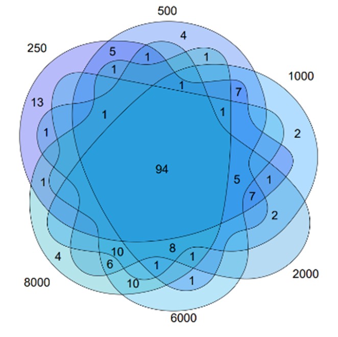
References
(1) Gebski, V., Garès, V., Gibbs, E. & Byth, K. Data maturity and follow-up in time-to-event analyses.International Journal of Epidemiology 47, 850–859 (2018).
-
- Oct 2025
-
www.biorxiv.org www.biorxiv.org
-
Author response:
The following is the authors’ response to the current reviews.
Reviewer #1 (Public review):
In this manuscript, Hoon Cho et al. present a novel investigation into the role of PexRAP, an intermediary in ether lipid biosynthesis, in B cell function, particularly during the Germinal Center (GC) reaction. The authors profile lipid composition in activated B cells both in vitro and in vivo, revealing the significance of PexRAP. Using a combination of animal models and imaging mass spectrometry, they demonstrate that PexRAP is specifically required in B cells. They further establish that its activity is critical upon antigen encounter, shaping B cell survival during the GC reaction. Mechanistically, they show that ether lipid synthesis is necessary to modulate reactive oxygen species (ROS) levels and prevent membrane peroxidation.
Highlights of the Manuscript:
The authors perform exhaustive imaging mass spectrometry (IMS) analyses of B cells, including GC B cells, to explore ether lipid metabolism during the humoral response. This approach is particularly noteworthy given the challenge of limited cell availability in GC reactions, which often hampers metabolomic studies. IMS proves to be a valuable tool in overcoming this limitation, allowing detailed exploration of GC metabolism.
The data presented is highly relevant, especially in light of recent studies suggesting a pivotal role for lipid metabolism in GC B cells. While these studies primarily focus on mitochondrial function, this manuscript uniquely investigates peroxisomes, which are linked to mitochondria and contribute to fatty acid oxidation (FAO). By extending the study of lipid metabolism beyond mitochondria to include peroxisomes, the authors add a critical dimension to our understanding of B cell biology.
Additionally, the metabolic plasticity of B cells poses challenges for studying metabolism, as genetic deletions from the beginning of B cell development often result in compensatory adaptations. To address this, the authors employ an acute loss-of-function approach using two conditional, cell-type-specific gene inactivation mouse models: one targeting B cells after the establishment of a pre-immune B cell population (Dhrs7b^f/f, huCD20-CreERT2) and the other during the GC reaction (Dhrs7b^f/f; S1pr2-CreERT2). This strategy is elegant and well-suited to studying the role of metabolism in B cell activation.
Overall, this manuscript is a significant contribution to the field, providing robust evidence for the fundamental role of lipid metabolism during the GC reaction and unveiling a novel function for peroxisomes in B cells.
Comments on revisions:
There are still some discrepancies in gating strategies. In Fig. 7B legend (lines 1082-1083), they show representative flow plots of GL7+ CD95+ GC B cells among viable B cells, so it is not clear if they are IgDneg, as the rest of the GC B cells aforementioned in the text.
We apologize for missing this item in need of correction in the revision and sincerely thank the reviewer for the stamina and care in picking this up. The data shown in Fig. 7B represented cells (events) in the IgD<sup>neg</sup> Dump<sup>neg</sup> viable lymphoid gate. We will correct this omission/blemish in the final revision that becomes the version of record.
Western blot confirmation: We understand the limitations the authors enumerate. Perhaps an RT-qPCR analysis of the Dhrs7b gene in sorted GC B cells from the S1PR2-CreERT2 model could be feasible, as it requires a smaller number of cells. In any case, we agree with the authors that the results obtained using the huCD20-CreERT2 model are consistent with those from the S1PR2-CreERT2 model, which adds credibility to the findings and supports the conclusion that GC B cells in the S1PR2-CreERT2 model are indeed deficient in PexRAP.
We will make efforts to go back through the manuscript and highlight this limitation to readers, i.e., that we were unable to get genetic evidence to assess what degree of "counter-selection" applied to GC B cells in our experiments.
We agree with the referee that optimally to support the Imaging Mass Spectrometry (IMS) data showing perturbations of various ether lipids within GC after depletion of PexRAP, it would have been best if we could have had a qRT2-PCR that allowed quantitation of the Dhrs7b-encoded mRNA in flow-purified GC B cells, or the extent to which the genomic DNA of these cells was in deleted rather than 'floxed' configuration.
While the short half-life of ether lipid species leads us to infer that the enzymatic function remains reduced/absent, it definitely is unsatisfying that the money for experiments ran out in June and the lab members had to move to new jobs.
Lines 222-226: We believe the correct figure is 4B, whereas the text refers to 4C.
As for the 1st item, we apologize and will correct this error.
Supplementary Figure 1 (line 1147): The figure title suggests that the data on T-cell numbers are from mice in a steady state. However, the legend indicates that the mice were immunized, which means the data are not from steady-state conditions.
We will change the wording both on line 1147 and 1152.
Reviewer #2 (Public review):
Summary:
In this study, Cho et al. investigate the role of ether lipid biosynthesis in B cell biology, particularly focusing on GC B cell, by inducible deletion of PexRAP, an enzyme responsible for the synthesis of ether lipids.
Strengths:
Overall, the data are well-presented, the paper is well-written and provides valuable mechanistic insights into the importance of PexRAP enzyme in GC B cell proliferation.
Weaknesses:
More detailed mechanisms of the impaired GC B cell proliferation by PexRAP deficiency remain to be further investigated. In minor part, there are issues for the interpretation of the data which might cause confusions by readers.
Comments on revisions:
The authors improved the manuscript appropriately according to my comments.
To re-summarize, we very much appreciate the diligence of the referees and Editors in re-reviewing this work at each cycle and helping via constructive peer review, along with their favorable comments and overall assessments. The final points will be addressed with minor edits since there no longer is any money for further work and the lab people have moved on.
The following is the authors’ response to the original reviews.
Reviewer #1 (Public review):
In this manuscript, Sung Hoon Cho et al. presents a novel investigation into the role of PexRAP, an intermediary in ether lipid biosynthesis, in B cell function, particularly during the Germinal Center (GC) reaction. The authors profile lipid composition in activated B cells both in vitro and in vivo, revealing the significance of PexRAP. Using a combination of animal models and imaging mass spectrometry, they demonstrate that PexRAP is specifically required in B cells. They further establish that its activity is critical upon antigen encounter, shaping B cell survival during the GC reaction.
Mechanistically, they show that ether lipid synthesis is necessary to modulate reactive oxygen species (ROS) levels and prevent membrane peroxidation.
Highlights of the Manuscript:
The authors perform exhaustive imaging mass spectrometry (IMS) analyses of B cells, including GC B cells, to explore ether lipid metabolism during the humoral response. This approach is particularly noteworthy given the challenge of limited cell availability in GC reactions, which often hampers metabolomic studies. IMS proves to be a valuable tool in overcoming this limitation, allowing detailed exploration of GC metabolism.
The data presented is highly relevant, especially in light of recent studies suggesting a pivotal role for lipid metabolism in GC B cells. While these studies primarily focus on mitochondrial function, this manuscript uniquely investigates peroxisomes, which are linked to mitochondria and contribute to fatty acid oxidation (FAO). By extending the study of lipid metabolism beyond mitochondria to include peroxisomes, the authors add a critical dimension to our understanding of B cell biology.
Additionally, the metabolic plasticity of B cells poses challenges for studying metabolism, as genetic deletions from the beginning of B cell development often result in compensatory adaptations. To address this, the authors employ an acute loss-of-function approach using two conditional, cell-type-specific gene inactivation mouse models: one targeting B cells after the establishment of a pre-immune B cell population (Dhrs7b^f/f, huCD20-CreERT2) and the other during the GC reaction (Dhrs7b^f/f; S1pr2-CreERT2). This strategy is elegant and well-suited to studying the role of metabolism in B cell activation.
Overall, this manuscript is a significant contribution to the field, providing robust evidence for the fundamental role of lipid metabolism during the GC reaction and unveiling a novel function for peroxisomes in B cells.
We appreciate these positive reactions and response, and agree with the overview and summary of the paper's approaches and strengths.
However, several major points need to be addressed:
Major Comments:
Figures 1 and 2
The authors conclude, based on the results from these two figures, that PexRAP promotes the homeostatic maintenance and proliferation of B cells. In this section, the authors first use a tamoxifen-inducible full Dhrs7b knockout (KO) and afterwards Dhrs7bΔ/Δ-B model to specifically characterize the role of this molecule in B cells. They characterize the B and T cell compartments using flow cytometry (FACS) and examine the establishment of the GC reaction using FACS and immunofluorescence. They conclude that B cell numbers are reduced, and the GC reaction is defective upon stimulation, showing a reduction in the total percentage of GC cells, particularly in the light zone (LZ).
The analysis of the steady-state B cell compartment should also be improved. This includes a more detailed characterization of MZ and B1 populations, given the role of lipid metabolism and lipid peroxidation in these subtypes.
Suggestions for Improvement:
B Cell compartment characterization: A deeper characterization of the B cell compartment in non-immunized mice is needed, including analysis of Marginal Zone (MZ) maturation and a more detailed examination of the B1 compartment. This is especially important given the role of specific lipid metabolism in these cell types. The phenotyping of the B cell compartment should also include an analysis of immunoglobulin levels on the membrane, considering the impact of lipids on membrane composition.
Although the manuscript is focused on post-ontogenic B cell regulation in Ab responses, we believe we will be able to polish a revised manuscript through addition of results of analyses suggested by this point in the review: measurement of surface IgM on and phenotyping of various B cell subsets, including MZB and B1 B cells, to extend the data in Supplemental Fig 1H and I. Depending on the level of support, new immunization experiments to score Tfh and analyze a few of their functional molecules as part of a B cell paper may be feasible.
Addendum / update of Sept 2025: We added new data with more on MZB and B1 B cells, surface IgM, and on Tfh populations.
GC Response Analysis Upon Immunization: The GC response characterization should include additional data on the T cell compartment, specifically the presence and function of Tfh cells. In Fig. 1H, the distribution of the LZ appears strikingly different. However, the authors have not addressed this in the text. A more thorough characterization of centroblasts and centrocytes using CXCR4 and CD86 markers is needed.
The gating strategy used to characterize GC cells (GL7+CD95+ in IgD− cells) is suboptimal. A more robust analysis of GC cells should be performed in total B220+CD138− cells.
We first want to apologize the mislabeling of LZ and DZ in Fig 1H. The greenish-yellow colored region (GL7<sup>+</sup> CD35<sup>+</sup>) indicate the DZ and the cyan-colored region (GL7<sup>+</sup> CD35<sup>+</sup>) indicates the LZ. Addendum / update of Sept 2025: We corrected the mistake, and added new experimental data using the CD138 marker to exclude preplasmablasts.
As a technical note, we experienced high background noise with GL7 staining uniquely with PexRAP deficient (Dhrs7b<sup>f/f</sup>; Rosa26-CreER<sup>T2</sup>) mice (i.e., not WT control mice). The high background noise of GL7 staining was not observed in B cell specific KO of PexRAP (Dhrs7b<sup>f/f</sup>; huCD20-CreER<sup>T2</sup>). Two formal possibilities to account for this staining issue would be if either the expression of the GL7 epitope were repressed by PexRAP or the proper positioning of GL7<sup>+</sup> cells in germinal center region were defective in PexRAPdeficient mice (e.g., due to an effect on positioning cues from cell types other than B cells). In a revised manuscript, we will fix the labeling error and further discuss the GL7 issue, while taking care not to be thought to conclude that there is a positioning problem or derepression of GL7 (an activation antigen on T cells as well as B cells).
While the gating strategy for an overall population of GC B cells is fairly standard even in the current literature, the question about using CD138 staining to exclude early plasmablasts (i.e., analyze B220<sup>+</sup> CD138<sup>neg</sup> vs B220<sup>+</sup> CD138<sup>+</sup>) is interesting. In addition, some papers like to use GL7<sup>+</sup> CD38<sup>neg</sup> for GC B cells instead of GL7<sup>+</sup> Fas (CD95)<sup>+</sup>, and we thank the reviewer for suggesting the analysis of centroblasts and centrocytes. For the revision, we will try to secure resources to revisit the immunizations and analyze them for these other facets of GC B cells (including CXCR4/CD86) and for their GL7<sup>+</sup> CD38<sup>neg</sup>. B220<sup>+</sup> CD138<sup>-</sup> and B220<sup>+</sup> CD138<sup>+</sup> cell populations.
We agree that comparison of the Rosa26-CreERT2 results to those with B cell-specific lossof-function raise a tantalizing possibility that Tfh cells also are influenced by PexRAP. Although the manuscript is focused on post-ontogenic B cell regulation in Ab responses, we hope to add a new immunization experiments that scores Tfh and analyzes a few of their functional molecules could be added to this B cell paper, depending on the ability to wheedle enough support / fiscal resources.
Addendum / update of Sept 2025: Within the tight time until lab closure, and limited $$, we were able to do experiments that further reinforced the GC B cell data - including stains for DZ vs LZ sub-subsetting - and analyzed Tfh cells. We were not able to explore changes in functional antigenic markers on the GC B or Tfh cells.
The authors claim that Dhrs7b supports the homeostatic maintenance of quiescent B cells in vivo and promotes effective proliferation. This conclusion is primarily based on experiments where CTV-labeled PexRAP-deficient B cells were adoptively transferred into μMT mice (Fig. 2D-F). However, we recommend reviewing the flow plots of CTV in Fig. 2E, as they appear out of scale. More importantly, the low recovery of PexRAP-deficient B cells post-adoptive transfer weakens the robustness of the results and is insufficient to conclusively support the role of PexRAP in B cell proliferation in vivo.
In the revision, we will edit the text and try to adjust the digitized cytometry data to allow more dynamic range to the right side of the upper panels in Fig. 2E, and otherwise to improve the presentation of the in vivo CTV result. However, we feel impelled to push back respectfully on some of the concern raised here. First, it seems to gloss over the presentation of multiple facets of evidence. The conclusion about maintenance derives primarily from Fig. 2C, which shows a rapid, statistically significant decrease in B cell numbers (extending the finding of Fig. 1D, a more substantial decrease after a bit longer a period). As noted in the text, the rate of de novo B cell production does not suffice to explain the magnitude of the decrease.
In terms of proliferation, we will improve presentation of the Methods but the bottom line is that the recovery efficiency is not bad (comparing to prior published work) inasmuch as transferred B cells do not uniformly home to spleen. In a setting where BAFF is in ample supply in vivo, we transferred equal numbers of cells that were equally labeled with CTV and counted B cells. The CTV result might be affected by lower recovered B cell with PexRAP deficiency, generally, the frequencies of CTV<sup>low</sup> divided population are not changed very much. However, it is precisely because of the pitfalls of in vivo analyses that we included complementary data with survival and proliferation in vitro. The proliferation was attenuated in PexRAP-deficient B cells in vitro; this evidence supports the conclusion that proliferation of PexRAP knockout B cells is reduced. It is likely that PexRAP deficient B cells also have defect in viability in vivo as we observed the reduced B cell number in PexRAP-deficient mice. As the reviewer noticed, the presence of a defect in cycling does, in the transfer experiments, limit the ability to interpret a lower yield of B cell population after adoptive transfer into µMT recipient mice as evidence pertaining to death rates. We will edit the text of the revision with these points in mind.
In vitro stimulation experiments: These experiments need improvement. The authors have used anti-CD40 and BAFF for B cell stimulation; however, it would be beneficial to also include antiIgM in the stimulation cocktail. In Fig. 2G, CTV plots do not show clear defects in proliferation, yet the authors quantify the percentage of cells with more than three divisions. These plots should clearly display the gating strategy. Additionally, details about histogram normalization and potential defects in cell numbers are missing. A more in-depth analysis of apoptosis is also required to determine whether the observed defects are due to impaired proliferation or reduced survival.
As suggested by reviewer, testing additional forms of B cell activation can help explore the generality (or lack thereof) of findings. We plan to test anti-IgM stimulation together with anti-CD40 + BAFF as well as anti-IgM + TLR7/8, and add the data to a revised and final manuscript.
Addendum / update of Sept 2025: The revision includes results of new experiments in which anti-IgM was included in the stimulation cocktail, as well as further data on apoptosis and distinguishing impaired cycling / divisions from reduced survival .
With regards to Fig. 2G (and 2H), in the revised manuscript we will refine the presentation (add a demonstration of the gating, and explicate histogram normalization of FlowJo).
It is an interesting issue in bioscience, but in our presentation 'representative data' really are pretty representative, so a senior author is reminded of a comment Tak Mak made about a reduction (of proliferation, if memory serves) to 0.7 x control. [His point in a comment to referees at a symposium related that to a salary reduction by 30% :) A mathematical alternative is to point out that across four rounds of division for WT cells, a reduction to 0.7x efficiency at each cycle means about 1/4 as many progeny.]
We will try to edit the revision (Methods, Legends, Results, Discussion] to address better the points of the last two sentences of the comment, and improve the details that could assist in replication or comparisons (e.g., if someone develops a PexRAP inhibitor as potential therapeutic).
For the present, please note that the cell numbers at the end of the cultures are currently shown in Fig 2, panel I. Analogous culture results are shown in Fig 8, panels I, J, albeit with harvesting at day 5 instead of day 4. So, a difference of ≥ 3x needs to be explained. As noted above, a division efficiency reduced to 0.7x normal might account for such a decrease, but in practice the data of Fig. 2I show that the number of PexRAP-deficient B cells at day 4 is similar to the number plated before activation, and yet there has been a reasonable amount of divisions. So cell numbers in the culture of mutant B cells are constant because cycling is active but decreased and insufficient to allow increased numbers ("proliferation" in the true sense) as programmed death is increased. In line with this evidence, Fig 8G-H document higher death rates [i.e., frequencies of cleaved caspase3<sup>+</sup> cell and Annexin V<sup>+</sup> cells] of PexRAP-deficient B cells compared to controls. Thus, the in vitro data lead to the conclusion that both decreased division rates and increased death operate after this form of stimulation.
An inference is that this is the case in vivo as well - note that recoveries differed by ~3x (Fig. 2D), and the decrease in divisions (presentation of which will be improved) was meaningful but of lesser magnitude (Fig. 2E, F).
Reviewer #2 (Public review):
Summary:
In this study, Cho et al. investigate the role of ether lipid biosynthesis in B cell biology, particularly focusing on GC B cell, by inducible deletion of PexRAP, an enzyme responsible for the synthesis of ether lipids.
Strengths:
Overall, the data are well-presented, the paper is well-written and provides valuable mechanistic insights into the importance of PexRAP enzyme in GC B cell proliferation.
We appreciate this positive response and agree with the overview and summary of the paper's approaches and strengths.
Weaknesses:
More detailed mechanisms of the impaired GC B cell proliferation by PexRAP deficiency remain to be further investigated. In the minor part, there are issues with the interpretation of the data which might cause confusion for the readers.
Issues about contributions of cell cycling and divisions on the one hand, and susceptibility to death on the other, were discussed above, amplifying on the current manuscript text. The aggregate data support a model in which both processes are impacted for mature B cells in general, and mechanistically the evidence and work focus on the increased ROS and modes of death. Although the data in Fig. 7 do provide evidence that GC B cells themselves are affected, we agree that resource limitations had militated against developing further evidence about cycling specifically for GC B cells. We will hope to be able to obtain sufficient data from some specific analysis of proliferation in vivo (e.g., Ki67 or BrdU) as well as ROS and death ex vivo when harvesting new samples from mice immunized to analyze GC B cells for CXCR4/CD86, CD38, CD138 as indicated by Reviewer 1. As suggested by Reviewer 2, we will further discuss the possible mechanism(s) by which proliferation of PexRAP-deficient B cells is impaired. We also will edit the text of a revision where to enhance clarity of data interpretation - at a minimum, to be very clear that caution is warranted in assuming that GC B cells will exhibit the same mechanisms as cultures in vitro-stimulated B cells.
Addendum / update of Sept 2025: We were able to obtain results of intravital BrdU incorporation into GC B cells to measure cell cycling rates. The revised manuscript includes these results as well as other new data on apoptosis / survival, while deleting the data about CD138 populations whose interpretation was reasonably questioned by the referees.
Reviewer #1 (Recommendations for the authors):
We believe the evidence presented to support the role of PexRAP in protecting B cells from cell death and promoting B cell proliferation is not sufficiently robust and requires further validation in vivo. While the study demonstrates an increase in ether lipid content within the GC compartment, it also highlights a reduction in mature B cells in PexRAP-deficient mice under steady-state conditions. However, the IMS results (Fig. 3A) indicate that there are no significant differences in ether lipid content in the naïve B cell population. This discrepancy raises an intriguing point for discussion: why is PexRAP critical for B cell survival under steady-state conditions?
We thank the referee for all their care and input, and we agree that further intravital analyses could strengthen the work by providing more direct evidence of impairment of GC B cells in vivo. To revise and improve this manuscript before creation of a contribution of record, we performed new experiments to the limit of available funds and have both (i) added these new data and (ii) sharpened the presentation to correct what we believe to be one inaccurate point raised in the review.
(A) Specifically, we immunized mice with a B cell-specific depletion of PexRAP (Dhrs7b<sup>D/D-B</sup> mice) and measured a variety of readouts of the GC B cells' physiology in vivo: proliferation by intravital incorporation of BrdU, ROS in the viable GC B cell gate, and their cell death by annexin V staining directly ex vivo. Consistent with the data with in vitro activated B cells, these analyses showed increased ROS (new - Fig. 7D) and higher frequencies of Annexin V<sup>+</sup> 7AAD<sup>+</sup> in GC B cells (GL7<sup>+</sup> CD38<sup>-</sup> B cell-gate) of immunized Dhrs7b<sup>D/D-B</sup> mice compared with WT controls (huCD20-CreERT2<sup>+/-</sup>, Dhrs7b<sup>+/+</sup>) (new - Fig. 7E). Collectively, these results indicate that PexRAP aids (directly or indirectly) in controlling ROS in GC B cells and reduces B cell death, likely contributing to the substantially decreased overall GC B cell population. These new data are added to the revised manuscript in Figure 7.
Moreover, in each of two independent experiments (each comprising 3 vs 3 immunized mice), BrdU<sup>+</sup> events among GL7<sup>+</sup> CD38<sup>-</sup> (GC B cell)-gated cells were reduced in the B cell-specific PexRAP knockouts compared with WT controls (new, Fig. 7F and Supplemental Fig 6E). This result on cell cycle rates in vivo is presented with caution in the revised manuscript text because the absolute labeling fractions were somewhat different in Expt 1 vs Expt 2. This situation affords a useful opportunity to comment on the culture of "P values" and statistical methods. It is intriguing to consider how many successful drugs are based on research published back when the standard was to interpret a result of this sort more definitively despite a merged "P value" that was not a full 2 SD different from the mean. In the optimistic spirit of the eLife model, it can be for the attentive reader to decide from the data (new, Fig. 7F and Supplemental Fig 6E) whether to interpret the BrdU results more strongly that what we state in the revised text.
(B) On the issue of whether or not the loss of PexRAP led to perturbations of the lipidome of B cells prior to activation, we have edited the manuscript to do a better job making this point more clear.
We point out to readers that in the resting, pre-activation state abnormalities were detected in naive B cells, not just in activated and GC B cells. In brief, the IMS analysis and LC-MS-MS analysis detected statistically significant differences in some, but not all, the ether phospholipids species in PexRAP deficient cells (some of which was in Supplemental Figure 2 of the original version).
With this appropriate and helpful concern having been raised, we realize that this important point merited inclusion in the main figures. We point specifically to a set of phosphatidyl choline ions shown in Fig. 3 (revised - panels A, B, D) of the revised manuscript (PC O-36:5; PC O-38:5; PC O-40:6 and -40:7).
For this ancillary record (because a discourse on the limitations of each analysis), we will note issues such as the presence of many non-B cells in each pixel of the IMS analyses (so that some or many "true positives" will fail to achieve a "significant difference") and for the naive B cells, differential rates of synthesis, turnover, and conversion (e.g., addition of another 2-carbon unit or saturation / desaturation of one side-chain). To the extent the concern reflects some surprise and perhaps skepticism that what seem relatively limited differences (many species appear unaffected, etc), we share in the sentiment. But the basic observation is that there are differences, and a reasonable connection between the altered lipid profile and evidence of effects on survival or proliferation (i.e., integration of survival and cell cycling / division).
Additionally, it would be valuable to evaluate the humoral response in a T-independent setting. This would clarify whether the role of PexRAP is restricted to GC B cells or extends to activated B cells in general.
We agree that this additional set of experiments would be nice and would extend work incrementally by testing the generality of the findings about Ab responses. The practical problem is that money and time ran out while testing important items that strengthen the evidence about GC B cells.
Finally, the manuscript would benefit from a thorough revision to improve its readability and clarity. Including more detailed descriptions of technical aspects, such as the specific stimuli and time points used in analyses, would greatly enhance the flow and comprehension of the study. Furthermore, the authors should review figure labeling to ensure consistency throughout the manuscript, and carefully cite the relevant references. For instance, S1PR2 CreERT2 mouse is established by Okada and Kurosaki (Shinnakasu et al ,Nat. Immunol, 2016)
We appreciate this feedback and comment, inasmuch as both the clarity and scholarship matter greatly to us for a final item of record. For the revision, we have given our best shot to editing the text in the hopes of improved clarity, reduction of discrepancies (helpfully noted in the Minor Comments), and further detail-rich descriptions of procedures. We also edited the figure labeling to give a better consistency. While we note that the appropriate citation of Shinnakasu et al (2016) was ref. #69 of the original and remains as a citation, we have rechecked other referencing and try to use citations with the best relevant references.
Minor Comments: The labeling of plots in Fig. 2 should be standardized. For example, in Fig. 2C, D, and G, the same mouse strain is used, yet the Cre+ mouse is labeled differently in each plot.
We agree and have tried to tighten up these features in the panels noted as well as more generally (e.g., Fig. 4, 5, 6, 7, 9; consistency of huCD20-CreERT2 / hCD20CreERT2).
According to the text, the results shown in Fig. 1G and H correspond to a full KO (Dhrs7b^f/f; Rosa26-CreERT2 mice). However, Fig. 1H indicates that the bottom image corresponds to Dhrs7b^f/f, huCD20-CreERT2 mice (Dhrs7bΔ/Δ -B).
We have corrected Fig. 1H to be labeled as Dhrs7b<sup>Δ/Δ</sup> (with the data on Dhrs7b<sup>Δ/Δ-B</sup> presented in Supplemental Figure 4A, which is correctly labeled). Thank you for picking up this error that crept in while using copy/paste in preparation of figure panels and failing to edit out the "-B"!
Similarly, the gating strategy for GC cells in the text mentions IgD− cells, while the figure legend refers to total viable B cells. These discrepancies need clarification.
We believe we located and have corrected this issue in the revised manuscript.
Figures 3 and 4. The authors claim that B cell expression of PexRAP is required to achieve normal concentrations of ether phospholipids.
Suggestions for Improvement:
Lipid Metabolism Analysis: The analysis in Fig. 3 is generally convincing but could be strengthened by including an additional stimulation condition such as anti-IgM plus antiCD40. In Fig. 4C, the authors display results from the full KO model. It would be helpful to include quantitative graphs summarizing the parameters displayed in the images.
We have performed new experiments (anti-IgM + anti-CD40) and added the data to the revised manuscript (new - Supplemental Fig. 2H and Supplemental Fig 6, D & F). Conclusions based on the effects are not changed from the original.
As a semantic comment and point of scientific process, any interpretation ("claim") can - by definition - only be taken to apply to the conditions of the experiment. Nonetheless, it is inescapable that at least for some ether P-lipids of naive, resting B cells, and for substantially more in B cells activated under the conditions that we outline, B cell expression of PexRAP is required.
With regards to the constructive suggestion about a new series of lipidomic analyses, we agree that for activated B cells it would be nice and increase insight into the spectrum of conditions under which the PexRAP-deficient B cells had altered content of ether phospholipids. However, in light of the costs of metabolomic analyses and the lack of funds to support further experiments, and the accuracy of the point as stated, we prioritized the experiments that could fit within the severely limited budget.
[One can add that our results provide a premise for later work to analyze a time course after activation, and to perform isotopomer (SIRM) analyses with [13] C-labeled acetate or glucose, so as to understand activation-induced increases in the overall To revise the manuscript, we did however extrapolate from the point about adding BCR cross-linking to anti-CD40 as a variant form of activating the B cells for measurements of ROS, population growth, and rates of division (CTV partitioning). The results of these analyses, which align with and thereby strengthen the conclusions about these functional features from experiments with anti-CD40 but no anti-IgM, are added to Supplemental Fig 2H and Supplemental Fig 6D, F.
Figures 5, 6, and 7
The authors claim that Dhrs7b in B cells shapes antibody affinity and quantity. They use two mouse models for this analysis: huCD20-CreERT2 and Dhrs7b f/f; S1pr2-CreERT2 mice.
Suggestions for Improvement:
Adaptive immune response characterization: A more comprehensive characterization of the adaptive immune response is needed, ideally using the Dhrs7b f/f; S1pr2-CreERT2 model. This should include: Analysis of the GC response in B220+CD138− cells. Class switch recombination analysis. A detailed characterization of centroblasts, centrocytes, and Tfh populations. Characterization of effector cells (plasma cells and memory cells).
Within the limits of time and money, we have performed new experiments prompted by this constructive set of suggestions.
Specifically, we analyzed the suggested read-outs in the huCD20-CreERT2, Dhrs7b<sup>f/f</sup> model after immunization, recognizing that it trades greater signal-noise for the fact that effects are due to a mix of the impact on B cells during clonal expansion before GC recruitment and activities within the GC. In brief, the results showed that
(a) the GC B cell population - defined as CD138<sup>neg</sup> GL7<sup>+</sup> CD38<sup>lo/neg</sup> IgD<sup>neg</sup> B cells - was about half as large for PexRAP-deficient B cells net of any early- or preplasmablasts (CD138<sup>+</sup> events) (new - Fig 5G);
(b) the frequencies of pre- / early plasmablasts (CD138<sup>+</sup> GL7<sup>+</sup> CD38<sup>neg</sup>) events (see new - Fig. 6H, I; also, new Supplemental Fig 5D) were so low as to make it unlikely that our data with the S1pr2-CreERT2 model (in Fig 7B, C) would be affected meaningfully by analysis of the CD138 levels;
(c) There was a modest decrease in centrocytes (LZ) but not centroblasts (DZ) (new - Fig 5H, I) - consistent with the immunohistochemical data of Supplemental Fig. 5A-C).
Because of time limitations (the "shelf life" of funds and the lab) and insufficient stock of the S1pr2-CreERT2, Dhrs7b<sup>f/f</sup> mice as well as those that would be needed as adoptive transfer recipients because of S1PR2 expression in (GC-)Tfh, the experiments were performed instead with the huCD20-CreERT2, Dhrs7b<sup>f/f</sup> model. We would also note that using this Cre transgene better harmonizes the centrocyte/centroblast and Tfh data with the existing data on these points in Supplemental Fig. 4.
(d) Of note, the analyses of Tfh and GC-Tfh phenotype cells using the huCD20-CreERT2 B cell type-specific inducible Cre system to inactivate Dhrs7b (new - Supplemental Fig 1G-I; which, along with new - Supplemental Fig 5E) provide evidence of an abnormality that must stem from a function or functions of PexRAP in B cells, most likely GC B cells. Specifically, it is known that the GC-Tfh population proliferates and is supported by the GC B cells, and the results of B cell-specific deletion show substantial reductions in Tfh cells (both the GC-Tfh gating and the wider gate for plots of CXCR5/PD-1/ fluorescence of CD4 T cells
Timepoint Consistency: The NP response (Fig. 5) is analyzed four weeks postimmunization, whereas SRBC (Supp. Fig. 4) and Fig. 7 are analyzed one week or nine days post-immunization. The NP system analysis should be repeated at shorter timepoints to match the peak GC reaction.
This comment may stem from a misunderstanding. As diagrammed in Fig. 5A, the experiments involving the NP system were in fact measured at 7 d after a secondary (booster) immunization. That timing is approximately the peak period and harmonizes with the 7 d used for harvesting SRBC-immunized mice. So in fact the data with each system were obtained at a similar time point. Of course the NP experiments involved a second immunization so that many plasma cell and Ab responses derived from memory B cells generated by the primary immunization. However, the field at present is dominated by the view that the vast majority of the GC B cells after this second immunization (which historically we perform with alum adjuvant) are recruited from the naive rather than the memory B cell pool. For the revised manuscript, we have taken care that the Methods, Legend, and Figure provide the information to readers, and expanded the statement of a rationale.
It may seem a technicality but under NIH regulations we are legally obligated to try to minimize mouse usage. It also behooves researchers to use funds wisely. In line with those imperatives, we used systems that would simultaneously allow analyses of GC B cells, identification of affinity maturation (which is minimal in our hands at a 7 d time point after primary NP-carrier immunization), and a switched repertoire (also minimal), and where with each immunogen the GC were scored at 7-9 d after immunization (9 d refers to the S1pr2-CreERT2 experiments). Apart from the end of funding, we feel that what little might be learned from performing a series of experiments that involve harvests 7 d after a primary immunization with NP-ovalbumin cannot well be justified.
In vitro plasma cell differentiation: Quantification is missing for plasma cell differentiation in vitro (Supp. Fig. 4). The stimulus used should also be specified in the figure legend. Given the use of anti-CD40, differentiation towards IgG1 plasma cells could provide additional insights.
As suggested by reviewer, we have added the results of quantifying the in vitro plasma cell differentiation in Supplemental Fig 6B. Also, we edited the Methods and Supplemental Figure Legend to give detailed information of in vitro stimulation.
Proliferation and apoptosis analysis: The observed defects in the humoral response should be correlated with proliferation and apoptosis analyses, including Ki67 and Caspase markers.
As suggested by the review, we have performed new experiment and analyzed the frequencies of cell death by annexin V staining, and elected to use intravital uptake of BrdU as a more direct measurement of S phase / cell cycling component of net proliferation. The new results are now displayed in Figure 5 and Supplemental Fig. 5.
Western blot confirmation: While the authors have demonstrated the absence of PexRAP protein in the huCD20-CreERT2 model, this has not been shown in GC B cells from the Dhrs7b f/f; S1pr2-CreERT2 model. This confirmation is necessary to validate the efficiency of Dhrs7b deletion.
We were unable to do this for technical reasons expanded on below. For the revision, we have edited in a bit of text more explicitly to alert readers to the potential impact of counter-selection on interpretation of the findings with GC B cells. Before entering the GC, B cells have undergone many divisions, so if there were major pre-GC counterselection, in all likelihood the GC B cells would PexRAP-sufficient. To recap from the original manuscript and the new data we have added, IMS shows altered lipid profiles in the GC B cells and the literature indicates that the lipids are short-lived, requiring de novo resynthesis. The BrdU, ROS, and annexin V data show that GC B cells are abnormal. Accordingly, abnormal GC B cells represent the parsimonious or straightforward interpretation of the new results with GC-Tfh cell prevalence.
While we take these findings together to suggest that counterselection (i.e., a Western result showing normal levels of PexRAP in the GC B cells) seems unlikely, it is formally possible and would mean that the in situ defects of GC B cells arose due to environmental influences of the PexRAP-deficient B cells during the developmental history of the WT B cells observed in the GC.
Having noted all that, we understand that concerns about counter-selection are an issue if a reader accepts the data showing that mutant (PexRAP-deficient) B cells tend to proliferate less and die more readily. Indeed, one can speculate that were we also to perform competition experiments in which the Ighb, Cd45.2 B cells (WT or Dhrs7b D/D) are mixed with equal numbers of Igha, Cd45.1 competitors, the differences would become much greater. With this in mind, Western blotting of flow-purified GC B cells might give a sense of how much counter-selection has occurred.
That said, the Westerns need at least 2.5 x 10<sup>6</sup> B cells (those in the manuscript used five million, 5 x 10<sup>6</sup>) and would need replication. Taken together with the observation that ~200,000 GC B cells (on average) were measured in each B cell-specific knockout mouse after immunization (Fig. 1, Fig 5) and taking into account yields from sorting, each Western would require some 20-25 tamoxifen-injected ___-CreERT2, Dhrs7b f/f mice, and about half again that number as controls. The expiry of funds prohibited the time and costs of generating that many mice (>70) and flow-purified GC B cells.
Figure 8
The authors claim that Dhrs7b contributes to the modulation of ROS, impacting B cell proliferation.
Suggestions for Improvement:
GC ROS Analysis: The in vitro ROS analysis should be complemented by characterizing ROS and lipid peroxidation in the GC response using the Dhrs7b f/f; S1pr2-CreERT2 model. Flow cytometry staining with H2DCFDA, MitoSOX, Caspase-3, and Annexin V would allow assessment of ROS levels and cell death in GC B cells.
While subject to some of the same practical limits noted above, we have performed new experiments in line with this helpful input of the reviewer, and added the helpful new data to the revised manuscript. Specifically, in addition to the BrdU and phenotyping analyses after immunization of huCD20-CreER<sup>T2</sup>, Dhrs7b<sup>f/f</sup> mice, DCFDA (ROS), MitoSox, and annexin V signals were measured for GC B cells. Although the mitoSox signals did not significantly differ for PexRAP-deficient GCB, the ROS and annexin V signals were substantially increased. We added the new data to Figure 5 and Supplemental Figure 5. Together with the decreased in vivo BrdU incorporation in GC B cells from Dhrs7b<sup>D/D-B</sup> mice, these results are consistent with and support our hypothesis that PexRAP regulates B cell population growth and GC physiology in part by regulating ROS detoxification, survival and proliferation of B cells.
Quantification is missing in Fig. 8E, and Fig. 8F should use clearer symbols for better readability.
We added quantification for Fig 8E in Supplemental Fig 6E, and edited the symbols in Fig 8F for better readability.
Figure 9
The authors claim that Dhrs7b in B cells affects oxidative metabolism and ER mass. The results in this section are well-performed and convincing.
Suggestion for Improvement:
Based on the results, the discussion should elaborate on the potential role of lipids in antigen presentation, considering their impact on mitochondria and ER function.
We very much appreciate the praise of the tantalizing findings about oxidative metabolism and ER mass, and will accept the encouragement that we add (prudently) to the Discussion section to make note of the points mentioned by the Reviewer, particularly now that (with their encouragement) we have the evidence that B cell-specific loss of PexRAP (with the huCD20-CreERT2 deletion prior to immunization) resulted in decreased (GC-)Tfh and somewhat lower GC B cell proliferation.
Reviewer #2 (Recommendations for the authors):
The authors should investigate whether PexRAP-deficient GC B cells exhibit increased mitochondrial ROS and cell death ex vivo, as observed in in vitro cultured B cells.
We very much appreciate the work of the referee and their input. We addressed this helpful recommendation, in essence aligned with points from Reviewer 1, via new experiments (until the money ran out) and addition of data to the manuscript. To recap briefly, we found increased ROS in GC B cells along with higher fractions of annexin V positive cells; intriguingly, increased mtROS (MitoSox signal) was not detected, which contrasts with the results in activated B cells in vitro in a small way. To keep the text focused and not stray too far outside the foundation supported by data, this point may align with papers that provide evidence of differences between pre-GC and GC B cells (for instance with lack of Tfam or LDHA in B cells).
It remains unclear whether the impaired proliferation of PexRAP-deficient B cells is primarily due to increased cell death. Although NAC treatment partially rescued the phenotype of reduced PexRAP-deficient B cell number, it did not restore them to control levels. Analysis of the proliferation capacity of PexRAP-deficient B cells following NAC treatment could provide more insight into the cause of impaired proliferation.
To add to the data permitting an assessment of this issue, we performed new experiments in which B cells were activated (BCR and CD40 cross-linking), cultured, and both the change in population and the CTV partitioning were measured in the presence or absence of NAC. The results, added to the revision as Supplemental Fig 6FH, show that although NAC improved cell numbers for PexRAP-deficient cells relative to controls, this compound did not increase divisions at all. We infer that the more powerful effect of this lipid synthesis enzyme is to promote survival rather than division capacity.
Primary antibody responses were assessed at only one time point (day 20). It would be valuable to examine the kinetics of antibody response at multiple time points (0, 1w, 2w, 3w, for example) to better understand the temporal impact of PexRAP on antibody production.
We thank the reviewer for this suggestion. While it may be that the kinetic measurement of Ag-specific antibody level across multiple time points would provide an additional mechanistic clue into the of impact PexRAP on antibody production, the end of sponsored funding and imminent lab closure precluded performing such experiments.
CD138+ cell population includes both GC-experienced and GC-independent plasma cells (Fig. 7). Enumeration of plasmablasts, which likely consists of both PexRAP-deleted and undeleted cells (Fig. 7D and E), may mislead the readers such that PexRAP is dispensable for plasmablast generation. I would suggest removing these data and instead examining the number of plasmablasts in the experimental setting of Fig. 4A (huCD20-CreERT2-mediated deletion) to address whether PexRAP-deficiency affects plasmablast generation.
We have eliminated the figure panels in question, since it is accurate that in the absence of a time-stamping or marking approach we have a limited ability to distinguish plasma cells that arose prior to inactivation of the Dhrs7b gene in B cells. In addition, we performed new experiments that were used to analyze the "early plasmablast" phenotype and added those data to the revision (Supplemental Fig 5D).
-
-
www.biorxiv.org www.biorxiv.org
-
Author Response:
The following is the authors’ response to the previous reviews.
We carefully read through the second-round reviews and the additional reviews. To us, the review process is somewhat unusual and very much dominated by referee 2, who aggressively insists that we mixed up the trigeminal nucleus and inferior olive and that as a consequence our results are meaningless. We think the stance of referee 2 and the focus on one single issue (the alleged mix-up of trigeminal nucleus and inferior olive) is somewhat unfortunate, leaves out much of our findings and we debated at length on how to deal with further revisions. In the end, we decided to again give priority to addressing the criticism of referees 2, because it is hard to go on with a heavily attacked paper without resolving the matter at stake. The following is a summary of, what we did:
Additional experimental work:
(1) We checked if the peripherin-antibody indeed reliably identifies climbing fibers.
To this end, we sectioned the elephant cerebellum and stained sections with the peripherin-antibody. We find: (i) the cerebellar white matter is strongly reactive for peripherin-antibodies, (ii) cerebellar peripherin-antibody staining of has an axonal appearance. (iii) Cerebellar Purkinje cell somata appear to be ensheated by peripherin-antibody staining. (iv) We observed that the peripherin-antibody reactivity gradually decreases from Purkinje cell somata to the pia in the cerebellar molecular layer. This work is shown in our revised Figure 2. All these four features align with the distribution of climbing fibers (which arrive through the white matter, are axons, ensheat Purkinje cell somata, and innervate Purkinje cell proximally not reaching the pia). In line with previous work, which showed similar cerebellar staining patterns in several species (Errante et al. 1998), we conclude that elephant climbing fibers are strongly reactive for peripherin-antibodies.
(2) We delineated the elephant olivo-cerebellar tract.
The strong peripherin-antibody reactivity of elephant climbing fibers enabled us to delineate the elephant olivo-cerebellar tract. We find the elephant olivo-cerebellar tract is a strongly peripherin-antibody reactive, well-delineated fiber tract several millimeters wide and about a centimeter in height. The unstained olivo-cerebellar tract has a greyish appearance. In the anterior regions of the olivo-cerebellar tract, we find that peripherin-antibody reactive fibers run in the dorsolateral brainstem and approach the cerebellar peduncle, where the tract gradually diminishes in size, presumably because climbing fibers discharge into the peduncle. Indeed, peripherin-antibody reactive fibers can be seen entering the cerebellar peduncle. Towards the posterior end of the peduncle, the olivo-cerebellar disappears (in the dorsal brainstem directly below the peduncle. We note that the olivo-cerebellar tract was referred to as the spinal trigeminal tract by Maseko et al. 2013. We think the tract in question cannot be the spinal trigeminal tract for two reasons: (i) This tract is the sole brainstem source of peripherin-positive climbing fibers entering the peduncle/ the cerebellum; this is the defining characteristic of the olivo-cerebellar tract. (ii) The tract in question is much smaller than the trigeminal nerve, disappears posterior to where the trigeminal nerve enters the brainstem (see below), and has no continuity with the trigeminal nerve; the continuity with the trigeminal nerve is the defining characteristic of the spinal trigeminal tract, however.
The anterior regions of the elephant olivo-cerebellar tract are similar to the anterior regions of olivo-cerebellar tract of other mammals in its dorsolateral position and the relation to the cerebellar peduncle. In its more posterior parts, the elephant olivo-cerebellar tract continues for a long distance (~1.5 cm) in roughly the same dorsolateral position and enters the serrated nucleus that we previously identified as the elephant inferior olive. The more posterior parts of the elephant olivo-cerebellar tract therefore differ from the more posterior parts of the olivo-cerebellar tract of other mammals, which follows a ventromedial trajectory towards a ventromedially situated inferior olive. The implication of our delineation of the elephant olivo-cerebellar tract is that we correctly identified the elephant inferior olive.
(3) An in-depth analysis of peripherin-antibody reactivity also indicates that the trigeminal nucleus receives no climbing fiber input.
We also studied the peripherin-antibody reactivity in and around the trigeminal nucleus. We had also noted in the previous submission that the trigeminal nucleus is weakly positive for peripherin, but that the staining pattern is uniform and not the type of axon bundle pattern that is seen in the inferior olive of other mammals. To us, this observation already argued against the presence of climbing fibers in the trigeminal nucleus. We also noted that the myelin stripes of the trigeminal nucleus were peripherin-antibody-negative. In the context of our olivo-cerebellar tract tracing we now also scrutinized the surroundings of the trigeminal nucleus for peripherin-antibody reactivity. We find that the ventral brainstem surrounding the trigeminal nucleus is devoid of peripherin-antibody reactivity. Accordingly, no climbing fibers, (which we have shown to be strongly peripherin-antibody-positive, see our point 1) arrive at the trigeminal nucleus. The absence of climbing fiber input indicates that previous work that identified the (trigeminal) nucleus as the inferior olive (Maseko et al 2013) is unlikely to be correct.
(4) We characterized the entry of the trigeminal nerve into the elephant brain.
To better understand how trigeminal information enters the elephant’s brain, we characterized the entry of the trigeminal nerve. This analysis indicated to us that the trigeminal nerve is not continuous with the olivo-cerebellar tract (the spinal trigeminal tract of Maseko et al. 2013) as previously claimed by Maseko et al. 2013. We show some of this evidence in Referee-Figure 1 below. The reason we think the trigeminal nerve is discontinuous with the olivo-cerebellar tract is the size discrepancy between the two structures. We first show this for the tracing data of Maseko et al. 2013. In the Maseko et al. 2013 data the trigeminal nerve (Referee-Figure 1A, their plate Y) has 3-4 times the diameter of the olivocerebellar tract (the alleged spinal trigeminal tract, Referee-Figure 1B, their plate Z). Note that most if not all trigeminal fibers are thought to continue from the nerve into the trigeminal tract (see our rat data below). We plotted the diameter of the trigeminal nerve and diameter of the olivo-cerebellar (the spinal trigeminal tract according to Maseko et al. 2013) from the Maseko et al. 2013 data (Referee-Figure 1C) and we found that the olivocerebellar tract has a fairly consistent diameter (46 ± 9 mm2, mean ± SD). Statistical considerations and anatomical evidence suggest that the tracing of the trigeminal nerve into the olivo-cerebellar (the spinal trigeminal tract according to Maseko et al. 2013) is almost certainly wrong. The most anterior point of the alleged spinal trigeminal tract has a diameter of 51 mm2 which is more than 15 standard deviations different from the most posterior diameter (194 mm2) of the trigeminal tract. For this assignment to be correct three-quarters of trigeminal nerve fibers would have to spontaneously disappear, something that does not happen in the brain. We also made similar observations in the African elephant Bibi, where the trigeminal nerve (Referee-Figure 1D) is much larger in diameter than the olivocerebellar tract (Referee-Figure 1E). We could also show that the olivocerebellar tract disappears into the peduncle posterior to where the trigeminal nerve enters (Referee-Figure 1F). Our data are very similar to Maseko et al. indicating that their outlining of structures was done correctly. What appears to have been oversimplified, is the assignment of structures as continuous. We also quantified the diameter of the trigeminal nerve and the spinal trigeminal tract in rats (from the Paxinos & Watson atlas; Referee-Figure 1D); as expected we found the trigeminal nerve and spinal trigeminal tract diameters are essentially continuous.
In our hands, the trigeminal nerve does not continue into a well-defined tract that could be traced after its entry. In this regard, it differs both from the olivo-cerebellar tract of the elephant or the spinal trigeminal tract of the rodent, both of which are well delineated. We think the absence of a well-delineated spinal trigeminal tract in elephants might have contributed to the putative tracing error highlighted in our Referee-Figure 1A-C.
We conclude that a size mismatch indicates trigeminal fibers do not run in the olivo-cerebellar tract (the spinal trigeminal tract according to Maseko et al. 2013).
Author response image 1.
The trigeminal nerve is discontinuous with the olivo-cerebellar tract (the spinal trigeminal tract according to Maseko et al. 2013). A, Trigeminal nerve (orange) in the brain of African elephant LAX as delineated by Maseko et al. 2013 (coronal section; their plate Y). B, Most anterior appearance of the spinal trigeminal tract of Maseko et al. 2013 (blue; coronal section; their plate Z). Note the much smaller diameter of the spinal trigeminal tract compared to the trigeminal nerve shown in C, which argues against the continuity of the two structures. Indeed, our peripherin-antibody staining showed that the spinal trigeminal tract of Maseko corresponds to the olivo-cerebellar tract and is discontinuous with the trigeminal nerve. C, Plot of the trigeminal nerve and olivo-cerebellar tracts (the spinal trigeminal tract according to Maseko et al. 2013) diameter along the anterior-posterior axis. The trigeminal nerve is much larger in diameter than the olivocerebellar tract (the spinal trigeminal tract according to Maseko et al. 2013). C, D measurements, for which sections are shown in panels C and D respectively. The olivocerebellar tract (the spinal trigeminal tract according to Maseko et al. 2013) has a consistent diameter; data replotted from Maseko et al. 2013. At mm 25 the inferior olive appears. D, Trigeminal nerve entry in the brain of African elephant Bibi; our data, coronal section, the trigeminal nerve is outlined in orange, note the large diameter. E, Most anterior appearance of the olivo-cerebellar tract in the brain of African elephant Bibi; our data, coronal section, approximately 3 mm posterior to the section shown in A, the olivocerebellar tract is outlined in blue. Note the smaller diameter of the olivo-cerebellar tract compared to the trigeminal nerve, which argues against the continuity of the two structures. F, Plot of the trigeminal nerve and olivo-cerebellar tract diameter along the anterior-posterior axis. The nerve and olivo-cerebellar tract are discontinuous and the trigeminal nerve is much larger in diameter than the olivocerebellar tract (the spinal trigeminal tract according to Maseko et al. 2013); our data. D, E measurements, for which sections are shown in panels D and E respectively. At mm 27 the inferior olive appears. G, In the rat the trigeminal nerve is continuous in size with the spinal trigeminal tract. Data replotted from Paxinos and Watson.
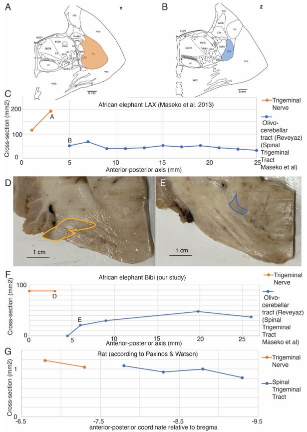
Reviewer 2 (Public Review):
As indicated in my previous review of this manuscript (see above), it is my opinion that the authors have misidentified, and indeed switched, the inferior olivary nuclear complex (IO) and the trigeminal nuclear complex (Vsens). It is this specific point only that I will address in this second review, as this is the crucial aspect of this paper - if the identification of these nuclear complexes in the elephant brainstem by the authors is incorrect, the remainder of the paper does not have any scientific validity.
Comment: We agree with the referee that it is most important to sort out, the inferior olivary nuclear complex (IO) and the trigeminal nuclear complex, respectively.Change: We did additional experimental work to resolve this matter as detailed at the beginning of our response. Specifically, we ascertained that elephant climbing fibers are strongly peripherin-positive. Based on elephant climbing fiber peripherin-reactivity we delineated the elephant olivo-cerebellar tract. We find that the olivo-cerebellar connects to the structure we refer to as inferior olive to the cerebellum (the referee refers to this structure as the trigeminal nuclear complex). We also found that the trigeminal nucleus (the structure the referee refers to as inferior olive) appears to receive no climbing fibers. We provide indications that the tracing of the trigeminal nerve into the olivo-cerebellar tract by Maseko et al. 2023 was erroneous (Author response image 1). These novel findings support our ideas but are very difficult to reconcile with the referee’s partitioning scheme.
The authors, in their response to my initial review, claim that I "bend" the comparative evidence against them. They further claim that as all other mammalian species exhibit a "serrated" appearance of the inferior olive, and as the elephant does not exhibit this appearance, that what was previously identified as the inferior olive is actually the trigeminal nucleus and vice versa.
For convenience, I will refer to IOM and VsensM as the identification of these structures according to Maseko et al (2013) and other authors and will use IOR and VsensR to refer to the identification forwarded in the study under review. <br /> The IOM/VsensR certainly does not have a serrated appearance in elephants. Indeed, from the plates supplied by the authors in response (Referee Fig. 2), the cytochrome oxidase image supplied and the image from Maseko et al (2013) shows a very similar appearance. There is no doubt that the authors are identifying structures that closely correspond to those provided by Maseko et al (2013). It is solely a contrast in what these nuclear complexes are called and the functional sequelae of the identification of these complexes (are they related to the trunk sensation or movement controlled by the cerebellum?) that is under debate.
Elephants are part of the Afrotheria, thus the most relevant comparative data to resolve this issue will be the identification of these nuclei in other Afrotherian species. Below I provide images of these nuclear complexes, labelled in the standard nomenclature, across several Afrotherian species.
(A) Lesser hedgehog tenrec (Echinops telfairi)
Tenrecs brains are the most intensively studied of the Afrotherian brains, these extensive neuroanatomical studies undertaken primarily by Heinz Künzle. Below I append images (coronal sections stained with cresol violet) of the IO and Vsens (labelled in the standard mammalian manner) in the lesser hedgehog tenrec. It should be clear that the inferior olive is located in the ventral midline of the rostral medulla oblongata (just like the rat) and that this nucleus is not distinctly serrated. The Vsens is located in the lateral aspect of the medulla skirted laterally by the spinal trigeminal tract (Sp5). These images and the labels indicating structures correlate precisely with that provide by Künzle (1997, 10.1016, see his Figure 1K,L. Thus, in the first case of a related species, there is no serrated appearance of the inferior olive, the location of the inferior olive is confirmed through connectivity with the superior colliculus (a standard connection in mammals) by Künzle (1997), and the location of Vsens is what is considered to be typical for mammals. This is in agreement with the authors, as they propose that ONLY the elephants show the variations they report.
(B) Giant otter shrew (Potomogale velox)
The otter shrews are close relatives of the Tenrecs. Below I append images of cresyl violet (left column) and myelin (right column) stained coronal sections through the brainstem with the IO, Vsens and Sp5 labelled as per standard mammalian anatomy. Here we see hints of the serration of the IO as defined by the authors, but we also see many myelin stripes across the IO. Vsens is located laterally and skirted by the Sp5. This is in agreement with the authors, as they propose that ONLY the elephants show the variations they report.
(C) Four-toed sengi (Petrodromus tetradactylus)
The sengis are close relatives of the Tenrecs and otter shrews, these three groups being part of the Afroinsectiphilia, a distinct branch of the Afrotheria. Below I append images of cresyl violet (left column) and myelin (right column) stained coronal sections through the brainstem with the IO, Vsens and Sp5 labelled as per standard mammalian anatomy. Here we see vague hints of the serration of the IO (as defined by the authors), and we also see many myelin stripes across the IO. Vsens is located laterally and skirted by the Sp5. This is in agreement with the authors, as they propose that ONLY the elephants show the variations they report.
(D) Rock hyrax (Procavia capensis)
The hyraxes, along with the sirens and elephants form the Paenungulata branch of the Afrotheria. Below I append images of cresyl violet (left column) and myelin (right column) stained coronal sections through the brainstem with the IO, Vsens and Sp5 labelled as per the standard mammalian anatomy. Here we see hints of the serration of the IO (as defined by the authors), but we also see evidence of a more "bulbous" appearance of subnuclei of the IO (particularly the principal nucleus), and we also see many myelin stripes across the IO. Vsens is located laterally and skirted by the Sp5. This is in agreement with the authors, as they propose that ONLY the elephants show the variations they report.
(E) West Indian manatee (Trichechus manatus)
The sirens are the closest extant relatives of the elephants in the Afrotheria. Below I append images of cresyl violet (top) and myelin (bottom) stained coronal sections (taken from the University of Wisconsin-Madison Brain Collection, https://brainmuseum.org, and while quite low in magnification they do reveal the structures under debate) through the brainstem with the IO, Vsens and Sp5 labelled as per standard mammalian anatomy. Here we see the serration of the IO (as defined by the authors). Vsens is located laterally and skirted by the Sp5. This is in agreement with the authors, as they propose that ONLY the elephants show the variations they report.
These comparisons and the structural identification, with which the authors agree as they only distinguish the elephants from the other Afrotheria, demonstrate that the appearance of the IO can be quite variable across mammalian species, including those with a close phylogenetic affinity to the elephants. Not all mammal species possess a "serrated" appearance of the IO. Thus, it is more than just theoretically possible that the IO of the elephant appears as described prior to this study.
So what about elephants? Below I append a series of images from coronal sections through the African elephant brainstem stained for Nissl, myelin, and immunostained for calretinin. These sections are labelled according to standard mammalian nomenclature. In these complete sections of the elephant brainstem, we do not see a serrated appearance of the IOM (as described previously and in the current study by the authors). Rather the principal nucleus of the IOM appears to be bulbous in nature. In the current study, no image of myelin staining in the IOM/VsensR is provided by the authors. However, in the images I provide, we do see the reported myelin stripes in all stains - agreement between the authors and reviewer on this point. The higher magnification image to the bottom left of the plate shows one of the IOM/VsensR myelin stripes immunostained for calretinin, and within the myelin stripes axons immunopositive for calretinin are seen (labelled with an arrow). The climbing fibres of the elephant cerebellar cortex are similarly calretinin immunopositive (10.1159/000345565). In contrast, although not shown at high magnification, the fibres forming the Sp5 in the elephant (in the Maseko description, unnamed in the description of the authors) show no immunoreactivity to calretinin.
Comment: We appreciate the referee’s additional comments. We concede the possibility that some relatives of elephants have a less serrated inferior olive than most other mammals. We maintain, however, that the elephant inferior olive (our Figure 1J) has the serrated appearance seen in the vast majority of mammals.
Change: None.
Peripherin Immunostaining
In their revised manuscript the authors present immunostaining of peripherin in the elephant brainstem. This is an important addition (although it does replace the only staining of myelin provided by the authors which is unusual as the word myelin is in the title of the paper) as peripherin is known to specifically label peripheral nerves. In addition, as pointed out by the authors, peripherin also immunostains climbing fibres (Errante et al., 1998). The understanding of this staining is important in determining the identification of the IO and Vsens in the elephant, although it is not ideal for this task as there is some ambiguity. Errante and colleagues (1998; Fig. 1) show that climbing fibres are peripherin-immunopositive in the rat. But what the authors do not evaluate is the extensive peripherin staining in the rat Sp5 in the same paper (Errante et al, 1998, Fig. 2). The image provided by the authors of their peripherin immunostaining (their new Figure 2) shows what I would call the Sp5 of the elephant to be strongly peripherin immunoreactive, just like the rat shown in Errant et al (1998), and more over in the precise position of the rat Sp5! This makes sense as this is where the axons subserving the "extraordinary" tactile sensitivity of the elephant trunk would be found (in the standard model of mammalian brainstem anatomy). Interestingly, the peripherin immunostaining in the elephant is clearly lamellated...this coincides precisely with the description of the trigeminal sensory nuclei in the elephant by Maskeo et al (2013) as pointed out by the authors in their rebuttal. Errante et al (1998) also point out peripherin immunostaining in the inferior olive, but according to the authors this is only "weakly present" in the elephant IOM/VsensR. This latter point is crucial. Surely if the elephant has an extraordinary sensory innervation from the trunk, with 400 000 axons entering the brain, the VsensR/IOM should be highly peripherin-immunopositive, including the myelinated axon bundles?! In this sense, the authors argue against their own interpretation - either the elephant trunk is not a highly sensitive tactile organ, or the VsensR is not the trigeminal nuclei it is supposed to be.
Comment: We made sure that elephant climbing fibers are strongly peripherin-positive (our revised Figure 2). As we noted in already our previous ms, we see weak diffuse peripherin-reactivity in the trigeminal nucleus (the inferior olive according to the referee), but no peripherin-reactive axon bundles (i.e. climbing fibers) that are seen in the inferior olive of other species. We also see no peripherin-reactive axon bundles (i.e. the olivo-cerebellar tract) arriving in the trigeminal nucleus as the tissue surrounding the trigeminal nucleus is devoid of peripherin-reactivity. Again, this finding is incompatible with the referee’s ideas. As far as we can tell, the trigeminal fibers are not reactive for peripherin in the elephant, i.e. we did not observe peripherin-reactivity very close to the nerve entry, but unfortunately, we did not stain for peripherin-reactivity into the nerve. As the referee alludes to the absence of peripherin-reactivity in the trigeminal tract is a difference between rodents and elephants.
Change: Our novel Figure 2.
Summary:
(1) Comparative data of species closely related to elephants (Afrotherians) demonstrates that not all mammals exhibit the "serrated" appearance of the principal nucleus of the inferior olive.
(2) The location of the IO and Vsens as reported in the current study (IOR and VsensR) would require a significant, and unprecedented, rearrangement of the brainstem in the elephants independently. I argue that the underlying molecular and genetic changes required to achieve this would be so extreme that it would lead to lethal phenotypes. Arguing that the "switcheroo" of the IO and Vsens does occur in the elephant (and no other mammals) and thus doesn't lead to lethal phenotypes is a circular argument that cannot be substantiated.
(3) Myelin stripes in the subnuclei of the inferior olivary nuclear complex are seen across all related mammals as shown above. Thus, the observation made in the elephant by the authors in what they call the VsensR, is similar to that seen in the IO of related mammals, especially when the IO takes on a more bulbous appearance. These myelin stripes are the origin of the olivocerebellar pathway, and are indeed calretinin immunopositive in the elephant as I show.
(4) What the authors see aligns perfectly with what has been described previously, the only difference being the names that nuclear complexes are being called. But identifying these nuclei is important, as any functional sequelae, as extensively discussed by the authors, is entirely dependent upon accurately identifying these nuclei.
(4) The peripherin immunostaining scores an own goal - if peripherin is marking peripheral nerves (as the authors and I believe it is), then why is the VsensR/IOM only "weakly positive" for this stain? This either means that the "extraordinary" tactile sensitivity of the elephant trunk is non-existent, or that the authors have misinterpreted this staining. That there is extensive staining in the fibre pathway dorsal and lateral to the IOR (which I call the spinal trigeminal tract), supports the idea that the authors have misinterpreted their peripherin immunostaining.
(5) Evolutionary expediency. The authors argue that what they report is an expedient way in which to modify the organisation of the brainstem in the elephant to accommodate the "extraordinary" tactile sensitivity. I disagree. As pointed out in my first review, the elephant cerebellum is very large and comprised of huge numbers of morphologically complex neurons. The inferior olivary nuclei in all mammals studied in detail to date, give rise to the climbing fibres that terminate on the Purkinje cells of the cerebellar cortex. It is more parsimonious to argue that, in alignment with the expansion of the elephant cerebellum (for motor control of the trunk), the inferior olivary nuclei (specifically the principal nucleus) have had additional neurons added to accommodate this cerebellar expansion. Such an addition of neurons to the principal nucleus of the inferior olive could readily lead to the loss of the serrated appearance of the principal nucleus of the inferior olive, and would require far less modifications in the developmental genetic program that forms these nuclei. This type of quantitative change appears to be the primary way in which structures are altered in the mammalian brainstem.
Comment: We still disagree with the referee. We note that our conclusions rest on the analysis of 8 elephant brainstems, which we sectioned in three planes and stained with a variety of metabolic and antibody stains and in which assigned two structures (the inferior olive and the trigeminal nucleus). Most of the evidence cited by the referee stems from a single paper, in which 147 structures were identified based on the analysis of a single brainstem sectioned in one plane and stained with a limited set of antibodies. Our synopsis of the evidence is the following.
(1) We agree with the referee that concerning brainstem position our scheme of a ventromedial trigeminal nucleus and a dorsolateral inferior olive deviates from the usual mammalian position of these nuclei (i.e. a dorsolateral trigeminal nucleus and a ventromedial inferior olive).
(2) Cytoarchitectonics support our partitioning scheme. The compact cellular appearance of our ventromedial trigeminal nucleus is characteristic of trigeminal nuclei. The serrated appearance of our dorsolateral inferior olive is characteristic of the mammalian inferior olive; we acknowledge that the referee claims exceptions here. To our knowledge, nobody has described a mammalian trigeminal nucleus with a serrated appearance (which would apply to the elephant in case the trigeminal nucleus is situated dorsolaterally).
(3) Metabolic staining (Cyto-chrome-oxidase reactivity) supports our partitioning scheme. Specifically, our ventromedial trigeminal nucleus shows intense Cyto-chrome-oxidase reactivity as it is seen in the trigeminal nuclei of trigeminal tactile experts.
(4) Isomorphism. The myelin stripes on our ventromedial trigeminal nucleus are isomorphic to trunk wrinkles. Isomorphism is a characteristic of somatosensory brain structures (barrel, barrelettes, nose-stripes, etc) and we know of no case, where such isomorphism was misleading.
(5) The large-scale organization of our ventromedial trigeminal nuclei in anterior-posterior repeats is characteristic of the mammalian trigeminal nuclei. To our knowledge, no such organization has ever been reported for the inferior olive.
(6) Connectivity analysis supports our partitioning scheme. According to our delineation of the elephant olivo-cerebellar tract, our dorsolateral inferior olive is connected via peripherin-positive climbing fibers to the cerebellum. In contrast, our ventromedial trigeminal nucleus (the referee’s inferior olive) is not connected via climbing fibers to the cerebellum.
Change: As discussed, we advanced further evidence in this revision. Our partitioning scheme (a ventromedial trigeminal nucleus and a dorsolateral inferior olive) is better supported by data and makes more sense than the referee’s suggestion (a dorsolateral trigeminal nucleus and a ventromedial inferior olive). It should be published.
Reviewer #3 (Public Review):
Summary:
The study claims to investigate trunk representations in elephant trigeminal nuclei located in the brainstem. The researchers identify large protrusions visible from the ventral surface of the brainstem, which they examined using a range of histological methods. However, this ventral location is usually where the inferior olivary complex is found, which challenges the author's assertions about the nucleus under analysis. They find that this brainstem nucleus of elephants contains repeating modules, with a focus on the anterior and largest unit which they define as the putative nucleus principalis trunk module of the trigeminal. The nucleus exhibits low neuron density, with glia outnumbering neurons significantly. The study also utilizes synchrotron X-ray phase contrast tomography to suggest that myelin-stripe-axons traverse this module. The analysis maps myelin-rich stripes in several specimens and concludes that based on their number and patterning that they likely correspond with trunk folds; however this conclusion is not well supported if the nucleus has been misidentified.
Comment: The referee provides a summary of our work. The referee also notes that the correct identification of the trigeminal nucleus is critical to the message of our paper.
Change: In line with these assessments we focused our revision efforts on the issue of trigeminal nucleus identification, please see our introductory comments and our response to Referee 2.
Strengths:
The strength of this research lies in its comprehensive use of various anatomical methods, including Nissl staining, myelin staining, Golgi staining, cytochrome oxidase labeling, and synchrotron X-ray phase contrast tomography. The inclusion of quantitative data on cell numbers and sizes, dendritic orientation and morphology, and blood vessel density across the nucleus adds a quantitative dimension. Furthermore, the research is commendable for its high-quality and abundant images and figures, effectively illustrating the anatomy under investigation.
Comment: We appreciate this positive assessment.
Change: None
Weaknesses:
While the research provides potentially valuable insights if revised to focus on the structure that appears to be inferior olivary nucleus, there are certain additional weaknesses that warrant further consideration. First, the suggestion that myelin stripes solely serve to separate sensory or motor modules rather than functioning as an "axonal supply system" lacks substantial support due to the absence of information about the neuronal origins and the termination targets of the axons. Postmortem fixed brain tissue limits the ability to trace full axon projections. While the study acknowledges these limitations, it is important to exercise caution in drawing conclusions about the precise role of myelin stripes without a more comprehensive understanding of their neural connections.
Comment: We understand these criticisms and the need for cautious interpretation. As we noted previously, we think that the Elife-publishing scheme, where critical referee commentary is published along with our ms, will make this contribution particularly valuable.
Change: Our additional efforts to secure the correct identification of the trigeminal nucleus.
Second, the quantification presented in the study lacks comparison to other species or other relevant variables within the elephant specimens (i.e., whole brain or brainstem volume). The absence of comparative data to different species limits the ability to fully evaluate the significance of the findings. Comparative analyses could provide a broader context for understanding whether the observed features are unique to elephants or more common across species. This limitation in comparative data hinders a more comprehensive assessment of the implications of the research within the broader field of neuroanatomy. Furthermore, the quantitative comparisons between African and Asian elephant specimens should include some measure of overall brain size as a covariate in the analyses. Addressing these weaknesses would enable a richer interpretation of the study's findings.
Comment: We understand, why the referee asks for additional comparative data, which would make our study more meaningful. We note that we already published a quantitative comparison of African and Asian elephant facial nuclei (Kaufmann et al. 2022). The quantitative differences between African and Asian elephant facial nuclei are similar in magnitude to what we observed here for the trigeminal nucleus, i.e. African elephants have about 10-15% more facial nucleus neurons than Asian elephants. The referee also notes that data on overall elephant brain size might be important for interpreting our data. We agree with this sentiment and we are preparing a ms on African and Asian elephant brain size. We find – unexpectedly given the larger body size of African elephants – that African elephants have smaller brains than Asian elephants. The finding might imply that African elephants, which have more facial nucleus neurons and more trigeminal nucleus trunk module neurons, are neurally more specialized in trunk control than Asian elephants.
Change: We are preparing a further ms on African and Asian elephant brain size, a first version of this work has been submitted.
Reviewer #4 (Public Review):
Summary:
The authors report a novel isomorphism in which the folds of the elephant trunk are recognizably mapped onto the principal sensory trigeminal nucleus in the brainstem. Further, they identifiy the enlarged nucleus as being situated in this species in an unusual ventral midline position.
Comment: The referee summarizes our work.
Change: None.
Strengths:
The identity of the purported trigeminal nucleus and the isomorphic mapping with the trunk folds is supported by multiple lines of evidence: enhanced staining for cytochrome oxidase, an enzyme associated with high metabolic activity; dense vascularization, consistent with high metabolic activity; prominent myelinated bundles that partition the nucleus in a 1:1 mapping of the cutaneous folds in the trunk periphery; near absence of labeling for the anti-peripherin antibody, specific for climbing fibers, which can be seen as expected in the inferior olive; and a high density of glia.
Comment: The referee again reviews some of our key findings.
Change: None.
Weaknesses:
Despite the supporting evidence listed above, the identification of the gross anatomical bumps, conspicuous in the ventral midline, is problematic. This would be the standard location of the inferior olive, with the principal trigeminal nucleus occupying a more dorsal position. This presents an apparent contradiction which at a minimum needs further discussion. Major species-specific specializations and positional shifts are well-documented for cortical areas, but nuclear layouts in the brainstem have been considered as less malleable.
Comment: The referee notes that our discrepancy with referee 2, needs to be addressed with further evidence and discussion, given the unusual position of both inferior olive and trigeminal nucleus in the partitioning scheme and that the mammalian brainstem tends to be positionally conservative. We agree with the referee. We note that – based on the immense size of the elephant trigeminal ganglion (50 g), half the size of a monkey brain – it was expected that the elephant trigeminal nucleus ought to be exceptionally large.
Change: We did additional experimental work to resolve this matter: (i) We ascertained that elephant climbing fibers are strongly peripherin-positive. (ii) Based on elephant climbing fiber peripherin-reactivity we delineated the elephant olivo-cerebellar tract. We find that the olivo-cerebellar connects to the structure we refer to as inferior olive to the cerebellum. (iii) We also found that the trigeminal nucleus (the structure the referee refers to as inferior olive) appears to receive no climbing fibers. (iv) We provide indications that the tracing of the trigeminal nerve into the olivo-cerebellar tract by Maseko et al. 2023 was erroneous (Referee-Figure 1). These novel findings support our ideas.
Reviewer #5 (Public Review):
After reading the manuscript and the concerns raised by reviewer 2 I see both sides of the argument - the relative location of trigeminal nucleus versus the inferior olive is quite different in elephants (and different from previous studies in elephants), but when there is a large disproportionate magnification of a behaviorally relevant body part at most levels of the nervous system (certainly in the cortex and thalamus), you can get major shifting in location of different structures. In the case of the elephant, it looks like there may be a lot of shifting. Something that is compelling is that the number of modules separated but the myelin bands correspond to the number of trunk folds which is different in the different elephants. This sort of modular division based on body parts is a general principle of mammalian brain organization (demonstrated beautifully for the cuneate and gracile nucleus in primates, VP in most of species, S1 in a variety of mammals such as the star nosed mole and duck-billed platypus). I don't think these relative changes in the brainstem would require major genetic programming - although some surely exists. Rodents and elephants have been independently evolving for over 60 million years so there is a substantial amount of time for changes in each l lineage to occur.
I agree that the authors have identified the trigeminal nucleus correctly, although comparisons with more out groups would be needed to confirm this (although I'm not suggesting that the authors do this). I also think the new figure (which shows previous divisions of the brainstem versus their own) allows the reader to consider these issues for themselves. When reviewing this paper, I actually took the time to go through atlases of other species and even look at some of my own data from highly derived species. Establishing homology across groups based only on relative location is tough especially when there appears to be large shifts in relative location of structures. My thoughts are that the authors did an extraordinary amount of work on obtaining, processing and analyzing this extremely valuable tissue. They document their work with images of the tissue and their arguments for their divisions are solid. I feel that they have earned the right to speculate - with qualifications - which they provide.
Comment: The referee summarizes our work and appears to be convinced by the line of our arguments. We are most grateful for this assessment. We add, again, that the skeptical assessment of referee 2 will be published as well and will give the interested reader the possibility to view another perspective on our work.
Change: None.
Recommendations for the authors:
Reviewer #1 (Recommendations For The Authors):
With this manuscript being virtually identical to the previous version, it is possible that some of the definitive conclusions about having identified the elephant trigeminal nucleus and trunk representation should be moderated in a more nuanced manner, especially given the careful and experienced perspective from reviewers with first hand knowledge elephant neuroanatomy.
Comment: We agree that both our first and second revisions were very much centered on the debate of the correct identification of the trigeminal nucleus and that our ms did not evolve as much in other regards. This being said we agree with Referee 2 that we needed to have this debate. We also think we advanced important novel data in this context (the delineation of elephant olivo-cerebellar tract through the peripherin-antibody).
Changes: Our revised Figure 2.
The peripherin staining adds another level of argument to the authors having identified the trigeminal brainstem instead of the inferior olive, if differential expression of peripherin is strong enough to distinguish one structure from the other.
Comment: We think we showed too little peripherin-antibody staining in our previous revision. We have now addressed this problem.
Changes: Our revised Figure 2, i.e. the delineation of elephant olivo-cerebellar tract through the peripherin-antibody).
There are some minor corrections to be made with the addition of Fig. 2., including renumbering the figures in the manuscript (e.g., 406, 521).
I continue to appreciate this novel investigation of the elephant brainstem and find it an interesting and thorough study, with the use of classical and modern neuroanatomical methods.
Comment: We are thankful for this positive assessment.
Reviewer #2 (Recommendations For The Authors):
I do realise the authors are very unhappy with me and the reviews I have submitted. I do apologise if feelings have been hurt, and I do understand the authors put in a lot of hard work and thought to develop what they have; however, it is unfortunate that the work and thoughts are not correct. Science is about the search for the truth and sometimes we get it wrong. This is part of the scientific process and why most journals adhere to strict review processes of scientific manuscripts. As I said previously, the authors can use their data to write a paper describing and quantifying Golgi staining of neurons in the principal olivary nucleus of the elephant that should be published in a specialised journal and contextualised in terms of the motor control of the trunk and the large cerebellum of the elephant.
Comment: We appreciate the referee’s kind words. Also, no hard feelings from our side, this is just a scientific debate. In our experience, neuroanatomical debates are resolved by evidence and we note that we provide evidence strengthening our identification of the trigeminal nucleus and inferior olive. As far as we can tell from this effort and the substantial evidence accumulated, the referee is wrong.
Reviewer #4 (Recommendations For The Authors):
As a new reviewer, I have benefited from reading the previous reviews and Author response, even while having several new comments to add.
(1) The identification of the inferior olive and trigeminal nuclei is obviously center stage. An enlargement of the trigeminal nuclei is not necessarily problematic, given the published reports on the dramatic enlargement of the trigeminal nerve (Purkart et al., 2022). At issue is the conspicuous relocation of the trigeminal nuclei that is being promoted by Reveyaz et al. Conspicuous rearrangements are not uncommon; for example, primary sensory cortical fields in different species (fig. 1 in H.H.A. Oelschlager for dolphins; S. De Vreese et al. (2023) for cetaceans, L. Krubitzer on various species, in the context of evolution). The difficult point here concerns what looks like a rather conspicuous gross anatomical rearrangement, in BRAINSTEM - the assumption being that the brainstem bauplan is going to be specifically conservative and refractory to gross anatomical rearrangement.
Comment: We agree with the referee that the brainstem rearrangements are unexpected. We also think that the correct identification of nuclei needs to be at the center of our revision efforts.
Change: Our revision provided further evidence (delineation of the olivo-cerebellar tract, characterization of the trigeminal nerve entry) about the identity of the nuclei we studied.
Why would a major nucleus shift to such a different location? and how? Can ex vivo DTI provide further support of the correct identification? Is there other "disruption" in the brainstem? What occupies the traditional position of the trigeminal nuclei? An atlas-equivalent coronal view of the entire brainstem would be informative. The Authors have assembled multiple criteria to support their argument that the ventral "bumps" are in fact a translocated trigeminal principal nucleus: enhanced CO staining, enhanced vascularization, enhanced myelination (via Golgi stains and tomography), very scant labeling for a climbing fiber specific antibody ( anti-peripherin), vs. dense staining of this in the alternative structure that they identify as IO; and a high density of glia. Admittedly, this should be sufficient, but the proposed translocation (in the BRAINSTEM) is sufficiently startling that this is arguably NOT sufficient. <br /> The terminology of "putative" is helpful, but a more cogent presentation of the results and more careful discussion might succeed in winning over at least some of a skeptical readership.
Comment: We do not know, what led to the elephant brainstem rearrangements we propose. If the trigeminal nuclei had expanded isometrically in elephants from the ancestral pattern, one would have expected a brain with big lateral bumps, not the elephant brain with its big ventromedial bumps. We note, however, that very likely the expansion of the elephant trigeminal nuclei did not occur isometrically. Instead, the neural representation of the elephant nose expanded dramatically and in rodents the nose is represented ventromedially in the brainstem face representation. Thus, we propose a ‘ventromedial outgrowth model’ according to which the elephant ventromedial trigeminal bumps result from a ventromedially direct outgrowth of the ancestral ventromedial nose representation.
We advanced substantially more evidence to support our partitioning scheme, including the delineation of the olivo-cerebellar tract based on peripherin-reactivity. We also identified problems in previous partitioning schemes, such as the claim that the trigeminal nerve continues into the ~4x smaller olivocerebellar tract (Referee-Figure 1C, D); we think such a flow of fibers, (which is also at odds with peripherin-antibody-reactivity and the appearance of nerve and olivocerebellar tract), is highly unlikely if not physically impossible. With all that we do not think that we overstate our case in our cautiously presented ms.
Change: We added evidence on the identification of elephant trigeminal nuclei and inferior olive.
(2) Role of myelin. While the photos of myelin are convincing, it would be nice to have further documentation. Gallyas? Would antibodies to MBP work? What is the myelin distribution in the "standard" trigeminal nuclei (human? macaque or chimpanzee?). What are alternative sources of the bundles? Regardless, I think it would be beneficial to de-emphasize this point about the role of myelin in demarcating compartments. <br /> I would in fact suggest an alternative (more neutral) title that might highlight instead the isomorphic feature; for example, "An isomorphic representation of Trunk folds in the Elephant Trigeminal Nucleus." The present title stresses myelin, but figure 1 already focuses on CO. Additionally, the folds are actually mentioned almost in passing until later in the manuscript. I recommend a short section on these at the beginning of the Results to serve as a useful framework.
Here I'm inclined to agree with the Reviewer, that the Authors' contention that the myelin stipes serve PRIMARILY to separate trunk-fold domains is not particularly compelling and arguably a distraction. The point can be made, but perhaps with less emphasis. After all, the fact that myelin has multiple roles is well-established, even if frequently overlooked. In addition, the Authors might make better use of an extensive relevant literature related to myelin as a compartmental marker; for example, results and discussion in D. Haenelt....N. Weiskopf (eLife, 2023), among others. Another example is the heavily myelinated stria of Gennari in primate visual cortex, consisting of intrinsic pyramidal cell axons, but where the role of the myelination has still not been elucidated.
Comment: (1) Documentation of myelin. We note that we show further identification of myelinated fibers by the fluorescent dye fluomyelin in Figure 4B. We also performed additional myelin stains as the gold-myelin stain after the protocol of Schmued (Referee-Figure 2). In the end, nothing worked quite as well to visualize myelin-stripes as the bright-field images shown in Figure 4A and it is only the images that allowed us to match myelin-stripes to trunk folds. Hence, we focus our presentation on these images.
(2) Title: We get why the referee envisions an alternative title. This being said, we would like to stick with our current title, because we feel it highlights the major novelty we discovered.
(3) We agree with many of the other comments of the referee on myelin phenomenology. We missed the Haenelt reference pointed out by the referee and think it is highly relevant to our paper
Change: 1. Review image 2. Inclusion of the Haenelt-reference.
Author response image 2.
Myelin stripes of the elephant trunk module visualized by Gold-chloride staining according to Schmued. A, Low magnification micrograph of the trunk module of African elephant Indra stained with AuCl according to Schmued. The putative finger is to the left, proximal is to the right. Myelin stripes can easily be recognized. The white box indicates the area shown in B. B, high magnification micrograph of two myelin stripes. Individual gold-stained (black) axons organized in myelin stripes can be recognized.
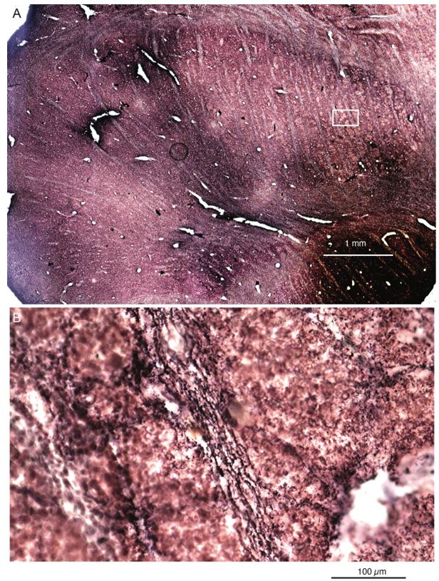
Schmued, L. C. (1990). A rapid, sensitive histochemical stain for myelin in frozen brain sections. Journal of Histochemistry & Cytochemistry,38(5), 717-720.
Are the "bumps" in any way "analogous" to the "brain warts" seen in entorhinal areas of some human brains (G. W. van Hoesen and A. Solodkin (1993)?
Comment: We think this is a similar phenomenon.
Change: We included the Hoesen and A. Solodkin (1993) reference in our discussion.
At least slightly more background (ie, a separate section or, if necessary, supplement) would be helpful, going into more detail on the several subdivisions of the ION and if these undergo major alterations in the elephant.
Comment: The strength of the paper is the detailed delineation of the trunk module, based on myelin stripes and isomorphism. We don’t think we have strong evidence on ION subdivisions, because it appears the trigeminal tract cannot be easily traced in elephants. Accordingly, we find it difficult to add information here.
Change: None.
Is there evidence from the literature of other conspicuous gross anatomical translocations, in any species, especially in subcortical regions?
Comment: The best example that comes to mind is the star-nosed mole brainstem. There is a beautiful paper comparing the star-nosed mole brainstem to the normal mole brainstem (Catania et al 2011). The principal trigeminal nucleus in the star-nosed mole is far more rostral and also more medial than in the mole; still, such rearrangements are minor compared to what we propose in elephants.
Catania, Kenneth C., Duncan B. Leitch, and Danielle Gauthier. "A star in the brainstem reveals the first step of cortical magnification." PloS one 6.7 (2011): e22406.
Change: None.
(3) A major point concerns the isomorphism between the putative trigeminal nuclei and the trunk specialization. I think this can be much better presented, at least with more discussion and other examples. The Authors mention about the rodent "barrels," but it seemed strange to me that they do not refer to their own results in pig (C. Ritter et al., 2023) nor the work from Ken Catania, 2002 (star-nosed mole; "fingerprints in the brain") or other that might be appropriate. I concur with the Reviewer that there should be more comparative data.
Comment: We agree.
Change: We added a discussion of other isomorphisms including the the star-nosed mole to our paper.
(4) Textual organization could be improved.
The Abstract all-important Introduction is a longish, semi "run-on" paragraph. At a minimum this should be broken up. The last paragraph of the Introduction puts forth five issues, but these are only loosely followed in the Results section. I think clarity and good organization is of the upmost importance in this manuscript. I recommend that the Authors begin the Results with a section on the trunk folds (currently figure 5, and discussion), continue with the several points related to the identification of the trigeminal nuclei, and continue with a parallel description of ION with more parallel data on the putative trigeminal and IO structures (currently referee Table 1, but incorporate into the text and add higher magnification of nucleus-specific cell types in the IO and trigeminal nuclei). Relevant comparative data should be included in the Discussion.
Comment: 1. We agree with the referee that our abstract needed to be revised. 2. We also think that our ms was heavily altered by the insertion of the new Figure 2, which complemented Figure 1 from our first submission and is concerned with the identification of the inferior olive. From a standpoint of textual flow such changes were not ideal, but the revisions massively added to the certainty with which we identify the trigeminal nuclei. Thus, although we are not as content as we were with the flow, we think the ms advanced in the revision process and we would like to keep the Figure sequence as is. 3. We already noted above that we included additional comparative evidence.
Change: 1. We revised our abstract. 2. We added comparative evidence.
Reviewer #5 (Recommendations For The Authors):
The data is invaluable and provides insights into some of the largest mammals on the planet.
Comment: We are incredibly thankful for this positive assessment.
-
-
www.biorxiv.org www.biorxiv.org
-
Author response:
The following is the authors’ response to the original reviews.
Reviewer 1:
Comment 0: In this paper, the authors develop a comprehensive program to investigate the organization of chromosome structures at 100 kb resolution. It is extremely well executed. The authors have thought through all aspects of the problem. The resulting software will be most useful to the community. Interestingly they capture many experimental observations accurately.
I have very few complaints.
We appreciate the reviewer’s strong assessment of the paper’s significance, novelty, and broad interest, and we thank them for the detailed suggestions and comments.
Comment 1: The number of parameters in the energy function is very large. Is there any justification for this? Could they simplify the functions?
We extend our gratitude to the reviewer for their insightful remarks. The parameters within our model can be categorized into two groups: those governing chromosome-chromosome interactions and those governing chromosome-nuclear landmark interactions.
In terms of chromosome-chromosome interactions, the parameter count is relatively modest compared to the vast amount of Hi-C data available. For instance, while the whole-genome Hi-C matrix at the 100KB resolution encompasses approximately 303212 contacts, our model comprises merely six parameters for interactions among different compartments, along with 1000 parameters for the ideal potential. As outlined in the supporting information, the ideal potential is contingent upon sequence separation, with 1000 chosen to encompass bead separations of up to 100MB. While it is theoretically plausible to reduce the number of parameters by assuming interactions cease beyond a certain sequence separation, determining this scale a priori presents a challenge.
During the parameterization process, we observed that interchromosomal contacts predicted solely based on compartmental interactions inadequately mirrored Hi-C data. Consequently, we introduced 231 additional parameters to more accurately capture interactions between distinct pairs of autosomes. These interactions may stem from factors such as non-coding RNA or proteins not explicable by simple, non-specific compartmental interactions.
Regarding parameters concerning chromosome-nuclear landmark interactions, we have 30321 parameters for speckles and 30321 for the nuclear lamina. To streamline the model, we opted to assign a unique parameter to each chromatin bead. However, it is conceivable that many chromatin beads share a similar mechanism for interacting with nuclear lamina or speckles, potentially allowing for a common parameter assignment. Nonetheless, implementing such simplification necessitates a deeper mechanistic understanding of chromosome-nuclear landmark interactions, an aspect currently lacking.
As our comprehension of nuclear organization progresses, the interpretability of parameter counts may improve, facilitating their reduction.
Comment 2: What would the modification be if the resolution is increased?
To increase the resolution of chromatin, we can in principle keep the same energy function as defined in Eq. S6. In this case, we only need to carry out further parameter optimization.
However, transitioning to higher resolutions may unveil additional features not readily apparent at 100kb. Notably, chromatin loops with an average size of 200kb or smaller have been identified in high-resolution Hi-C data [1]. To effectively capture these loops, new terms in the energy function must be incorporated. For instance, Qi and Zhang [2] employed additional contact potentials between CTCF sites to account for loop formation. Alternatively, an explicit loop-extrusion process could be introduced to model loop formation more accurately.
Comment 3: They should state that the extracted physical values are scale-dependent. For example, viscosity.
We thank the reviewer for the comment and would like to clarify that our model does not predict the viscosity. The nucleoplasmic viscosity was set as 1Pa · s to produce a diffusion coefficient that reproduces experimental value. The exact value for the nucleoplasmic viscosity is still rather controversial, and our selected value falls in the range of reported experimental values from 10−1Pa·s to 102Pa · s.
We have modified the main text to clarify the calculation of the diffusion coefficient.
“The exponent and the diffusion coefficient Dα = (27±11)×10−4μm2 · s−α both match well with the experimental values [cite], upon setting the nucleoplasmic viscosity as 1Pa · s (see Supporting Information Section: Mapping the reduced time unit to real time for more details).”
Reviewer 2:
Comment 0: In this work, Lao et al. develop an open-source software (OpenNucleome) for GPU-accelerated molecular dynamics simulation of the human nucleus accounting for chromatin, nucleoli, nuclear speckles, etc. Using this, the authors investigate the steady-state organization and dynamics of many of the nuclear components.
We thank the reviewer for summary of our work.
Comment 1: The authors could introduce a table having every parameter and the optimal parameter value used. This would greatly help the reader.
We would like to point out that model parameters are indeed provided in Table S1, S2, S3, S4, and Fig. S7. In these tables, we further provided details on how the parameters were determined.
Given the large number of parameters for the ideal potential (1000), we opted to plot it rather than listing out all the numbers. We added three new figures to plot the interaction parameters between chromosomes, between chromosomes and speckles, and between chromosomes and the nuclear lamina. Numerical values can be found online in the GitHub repository (parameters).
Comment 2: How many total beads are simulated? Do all beads have the same size?
The total number of the coarse-grained beads is 70542, including 60642 chromatin beads, 300 nucleolus beads, 1600 speckle beads, and 8000 nuclear lamina beads. The radius of the chromatin, nucleolus, and speckle beads is 0.25, while that of the lamina bead is 0.5. More information of the size and number of the beads are discussed in the Section: Components of the whole nucleus model.
Comment 3: In Equation S17, what is the 3rd and 4th powers mean? What necessitates it?
The potential defined in Equation S17 follows the definition of class2 bond in the LAMMPS package (LAMMPS docs). Compared to a typical harmonic potential, the presence of higher order terms produces sharper increase in the energy at large distances (Author response image 1). This essentially reduces the flucatuation of bond length in simulations.
Author response image 1.
Comparison between the Class2 potential (defined in Eq. S17) and the Harmonic potential (K(r − r0)2, with K = 20 and r0 = 0.5).
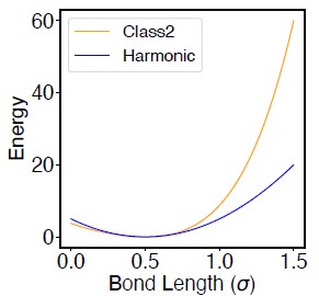
Comment 4: What do the X-axis and Y-axis numbers in Figure 5A and 5B mean? What are their units?
We apologize for the lack of clarify in our original figure. In Fig. 5A, the X and Y axis depicts the simulated and experimental radius of gyration (Rg) for individual chromosomes, as indicated in the title of the figure. Similarly, in Fig. 5B, the X and Y axis depicts the simulated and experimental radial position of individual chromosomes.
We have converted the chromosome Rg values into reduced units and labeled the corresponding axes in the updated figure (Fig. 5). The normalized radial position is unitless and its detailed definition is included in the supporting information Section: Computing simulated normalized chromosome radial positions. We updated the figure caption to provide an explicit reference to the SI text.
Reviewer 3:
Comment 0: In this work, the authors present the development of OpenNucleome, a software for simulating the structure and dynamics of the human nucleus. It provides a detailed model of nuclear components such as chromosomes and nuclear bodies, and uses GPU acceleration for better performance based on the OpenMM package. The work also shows the model’s accuracy in comparisons with experimental data and highlights the utility in the understanding of nuclear organization. While I consider this work a good tool for the genome architecture scientific community, I have some comments and questions that could further clarify the usage of this tool and help potential users. I also have a few questions that would help to clarify the technique and results and some suggestions for references.
We appreciate the reviewer’s strong assessment of the paper’s significance, novelty, and broad interest, and we thank them for the detailed suggestions and comments.
Comment 1: Could the authors elaborate on what they consider to be ’well-established and easily adoptable modeling tools’?
By well established, we meant that models that have been extensively validated and verified, and are highly regarded by the community.
By easily adoptable, we meant that tools that are well documented and can be relatively easily learned by new groups without help from the developers.
We have revised the text to clarify our meaning.
“Despite the progress made in computational modeling, the absence of well-documented software with easy-to-follow tutorials pose a challenge.”
Comment 2: Recognizing the value of a diverse range of tools in the community, the Open-MiChroM tool is also an open-source platform built on top of OpenMM. The documentation shows various modeling approaches and many tutorials that contain different approaches besides the MiChroM energy function. How does OpenNucleome compare in terms of facilitating crossvalidation and user accessibility? The two tools seem to be complementary, which is a gain to the field. I recommend adding one or two sentences in the matter. Also, while navigating the OpenNucleome GitHub, I have not found the tutorials mentioned in the text. I also consider a barrier in the process of generating necessary input files. I would suggest expanding the tutorials and documentation to help potential users.
We thank the reviewer for the excellent comments. We agree that while many of the tutorials were included in the original package, they were not as clearly documented. We have revised them extensively to to now present:
• A tutorial for optimizing chromosome chromosome interactions.
• A tutorial for optimizing chromosome nuclear landmark interactions.
• A tutorial for building initial configurations.
• A tutorial for relaxing the initial configurations.
• A tutorial for selecting the initial configurations.
• A tutorial for setting up performing Langevin dynamics simulations.
• A tutorial for setting up performing Brownian dynamics simulations.
• A tutorial for setting up performing simulations with deformed nucleus.
• A tutorial for analyzing simulation trajectories.
• A tutorial for introducing new features to the model.
These tutorials and our well-documented and open source code (https://zhanggroup-mitchemistry.github.io/OpenNucleome) should significantly promote user accessibility. Our inclusion of python scripts for analyzing simulation trajectorials shall allow users to compute various quantities for evaluating and comparing model quality.
We added a new paragraph in the Section: Conclusions and Dicussion of the main text to compare OpenNucleosome with existing software for genome modeling.
“Our software enhances the capabilities of existing genome simulation tools [cite]. Specifically, OpenNucleome aligns with the design principles of Open-MiChroM [cite], prioritizing open-source accessibility while expanding simulation capabilities to the entire nucleus. Similar to software from the Alber lab [cite], OpenNucleome offers highresolution genome organization that faithfully reproduces a diverse range of experimental data. Furthermore, beyond static structures, OpenNucleome facilitates dynamic simulations with explicit representations of various nuclear condensates, akin to the model developed by [citet].”
Comment 3: Lastly, I would appreciate it if the authors could expand their definition of ’standardized practices’.
We apologize for any confusion caused. By ”standardized practices,” we refer to the fact that different groups often employ unique procedures for structural modeling. These procedures differ in the representation of chromosomes, the nucleus environment, and the algorithms for parameter optimization. This absence of a consensus on the optimal practices for genome modeling can be daunting for newcomers to the field.
We have revised the text to the following to avoid confusion:
“Many research groups develop their own independent software, which complicates crossvalidation and hinders the establishment of best practices for genome modeling [3–5].”
Comment 4: On page 7, the authors refer to the SI Section: Components of the whole nucleus model for further details. Could the authors provide more information on the simulated density of nuclear bodies? Is there experimental data available that details the ratio of chromatin to other nuclear components, which was used as a reference in the simulation?
We thank the reviewer for the comment. Imaging studies have provided quantitative measures about the size and number of various nuclear bodies. For example, there are 2 ∼ 5 nucleoli per nucleus, with the typical size RNo ≈ 0.5μm [6–10]. In the review by Spector and Lamond [11], the authors showed that there are 20 ∼ 50 speckles, with the typical size RSp ≈ 0.3μm. We used these numbers to guide our simulation of nuclear bodies. These information was mentioned in the Section: Chromosomes as beads on the string polymers of the supporting information.
The chromatin density is fixed by the average size of chromatin bead and the nucleus size. We chose the size of chromatin based on imaging studies as detailed in the Subsection: Mapping chromatin bead size to real unit of the supporting information. Upon fixing the bead size, the chromatin volume is determined.
Comment 5: In the statement, ’the ideal potential is only applied for beads from the same chromosome to approximate the effect of loop extrusion by Cohesin molecules for chromosome compaction and territory formation,’ it would be helpful if the authors could clarify the scope of this potential. Specifically, the code indicates that the variable ’dend ideal’ is set at 1000, suggesting an interaction along a 100Mb polymer chain at a resolution of 100Kb per bead. Could the authors elaborate on their motivation for the Cohesin complex’s activity having a significant effect over such long distances within the polymer chain?
We thank the reviewer for the insight comment. They are correct that the ideal potential was introduced to capture chromosome folding beyond the interactions between compartments, including loop extrusion. Practically, we parameterized the ideal potential such that the simulated average contact probabilities as a function of sequence separation match the experimental values. The reviewer is correct that beyond a specific value of sequence separation, one would expect the impact of loop extrusion on chromosome folding should be negligible, due to Cohesin dissociation. Correspondingly, the interaction potential should be zero at large sequence separations.
However, it is important to note that the precise separation scale cannot be known a priori. We chose 100Mb as a conservative estimation. However, as we can see from Fig. S7, our parameterization scheme indeed produced interaction parameters are mainly zero at large sequence separations. Interesting, the scale at which the potential approaches 0 (∼ 500KB), indeed agree with the estimated length traveled by Cohesin molecules before dissociation [12].
Comment 6: On pages 8 and 9, the authors discuss the optimization process. However, in reviewing the code and documentation available on the GitHub page, I could not find specific sections related to the optimization procedure described in the paper. In this context, I have a few questions: Could the authors provide more details or direct me to the parts of the documentation and the text/SI that address the optimization procedure used in their study? Additional clarification on the cost/objective function employed during the optimization process would be highly beneficial, as this was not readily apparent in the text.
We thank the reviewer for the comment. We revised the SI to include the definition of the cost function for the Adam optimizer.
“During the optimization process, our aim was to minimize the disparity between experimental findings and simulated data. To achieve this, we defined the cost function as follows:
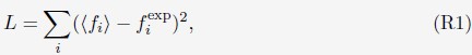
where the index i iterates over all the constraints defined in Eq. S28.”
The detailed optimization procedure was included in the SI as quoted below
“The details of the algorithm for parameter optimization are as follows
(1) Starting with a set of values for
 and
and  we performed 50 independent 3-million-step long MD simulations to obtain an ensemble of nuclear configurations. The 500K steps of each trajectory are discarded
as equilibration. We collected the configurations at every 2000 simulation steps from the rest of the simulation trajectories to compute the ensemble averages defined on the left-hand side of Eq. S13.
(2) Check the convergence of the optimization by calculating the percentage of error
defined as
 . The summation over i includes all the average contact probabilities defined in Eq. S28.
(3) If the error is less than a tolerance value etol, the optimization has converged, and we stop the simulations. Otherwise, we update the parameters, α, using the Adam optimizer [13]. With the new parameter values, we return to step one and restart the iteration.”
Previously, the optimization code was included as part of the analysis folder. To avoid confusion and improve readability, a separate folder named optimization has been created. This folder provides the Adam optimization of chromosome-chromosome interactions (chr-chr optimization) and chromosome-nuclear landmarks interactions (chr-NL optimization).
Comment 7: What was the motivation for choosing the Adam algorithm for optimization? Adam is designed for training on stochastic objective functions. Could the authors elucidate on the ’stochastic’ aspect of their function to be optimized? Why the Adam algorithm was considered the most appropriate choice for this application?
We thank the reviewer for the comment. As defined in Eq. R1, the cost function measures the difference between the simulated constraints with corresponding experimental values. The estimation of simulation values, by averaging over an ensemble of chromosome configurations, is inherently noisy and stochastic. Exact ensemble averages can only be achieved with unlimited samples obtained from infinite long simulations.
In the past, we have used the Newton’s method for parameterization, and the detailed algorithm can be found in the SI of Ref. 14. However, we found that Adam is more efficient as it is a first-order approximation method. The Newton’s method, on the other hand, is second-order approximation method and requires estimation of the Hessian matrix. When the number of constraints is large, as is in our case, the computational cost for estimating the Hessian matrix can be significant. Another advantage of the Adam algorithm lies in its adjustment of the learning rate along the optimization to further speedup convergence.
Comment 8: The authors mention that examples of setting up simulations, parameter optimization, and introducing new features are provided in the GitHub repository. However, I was unable to locate these examples. Could the authors guide me to these specific resources or consider adding them if they are not currently available?
We thank the reviewer for the comment. We have improved the GitHub repository and all the tutorials can be found using the links provided in Response to Comment 2.
Comment 9: Furthermore, the paper states that ’a configuration file that provides the position of individual particles in the PDB file format is needed to initialize the simulations.’ It would be beneficial for new users if the authors could elaborate on how this file is generated. And all other input files in general. Detailing the procedures for a new user to run their system using OpenNucleome would be helpful.
We thank the reviewer for the comment. The procedure for generating initial configurations was explained in the SI Section: Initial configurations for simulations and quoted below.
“We first created a total of 1000 configurations for the genome by sequentially generating the conformation of each one of the 46 chromosomes as follows. For a given chromosome, we start by placing the first bead at the center (origin) of the nucleus. The positions of the following beads, i, were determined from the (i − 1)-th bead as
 . v is a normalized random vector, and 0.5 was selected as the bond length between neighboring beads. To produce globular chromosome conformations, we rejected vectors, v, that led to bead positions with distance from the center larger than 4σ. Upon creating the conformation of a chromosome i, we shift its center of mass to a value ri com determined as follows. We first compute a mean radial distance,
  with the following equation
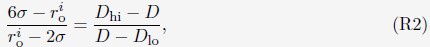
where Di is the average value of Lamin B DamID profile for chromosome i. Dhi and Dlo represent the highest and lowest average DamID values of all chromosomes, and 6σ and 2σ represent the upper and lower bound in radial positions for chromosomes. As shown in Fig. S6, the average Lamin B DamID profiles are highly correlated with normalized chromosome radial positions as reported by DNA MERFISH [cite], supporting their use as a proxy for estimating normalized chromosome radial positions. We then select
 as a uniformly distributed random variable within the range
  . Without loss of generality, we randomly chose the directions for shifting all 46 chromosomes.
We further relaxed the 1000 configurations to build more realistic genome structures. Following an energy minimization process, one-million-step molecular dynamics (MD) simulations were performed starting from each configuration. Simulations were performed with the following energy function

where UGenome is defined as in Eq. S7. UG-La is the excluded volume potential between chromosomes and lamina, i.e, only the second term in Eq. S24. Parameters in UGenome were from a preliminary optimization. The end configurations of the MD simulations were collected to build the final configuration ensemble (FCE).”
The tutorial for preparing initial configurations can be found at this link.
Comment 10: In the section discussing the correlation between simulated and experimental contact maps, as referenced in Figure 4A and Figure S2, the authors mention a high degree of correlation. Could the authors specify the exact value of this correlation and explain the method used for its computation? Considering that comparing two Hi-C matrices involves a large number of data points, it would be helpful to know if all data points were included in this analysis.
We have updated Fig 4A and S2 to include Pearson correlation coefficients next to the contact maps. The reviewer is correct in that all the non-redundant data points of the contact maps are included in computing the correlation coefficients.
For improved clarity, we added a new section in the supporting information to detail the calculations. The section is titled Computing Pearson correlation coefficients between experimental and simulated contact maps, and the relevant text is quoted below.
“We computed the Pearson correlation coefficients (PCC) between experimental and simulated contact maps in Fig. 4A and Fig. S2 as

xi and yi represent the experimental and simulated contact probabilities, and n is the total number of data points. Only non-redundant data points, i.e., half of the pairwise contacts, are used in the PCC calculation.”
Comment 11: In addition, the author said: ”Moreover, the simulated and experimental average contact probabilities between pairs of chromosomes agree well, and the Pearson correlation coefficient between the two datasets reaches 0.89.” How does this correlation behave when not accounting for polymer compaction or scaling? An analysis presenting the correlation as a function of genomic distance would be interesting.
Author response image 2.
Pearson correlation coefficient between experimental and simulated contact probabilities as a function of the sequence separation within specific chromosomes. For each chromosome, we first gathered a set of experimental contacts alongside a matching set of simulated ones for genomic pairs within a particular separation range. The Pearson correlation coefficient at the corresponding sequence separation was then determined using Equation R4. We limited the calculations to half of the chromosome length to ensure the availability of sufficient data.
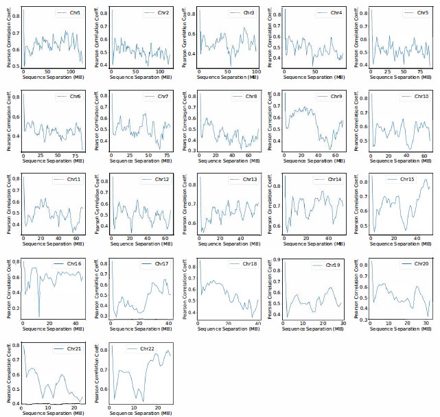
We thank the reviewer for the comment. The analysis presenting the correlation as a function of genomic distance (sequence separation) for each chromosome is shown in Figure S12 and also included in the SI. While the correlation coefficients decreases at larger separation, the values around 0.5 is quite reasonable and comparable to results obtained using Open-Michrom.
We also computed the correlation of whole genome contact maps after excluding intra-chromosomal contacts. The PCC decreased from 0.89 to 0.4. Again, the correlation coefficient is quite reasonable considering that these contacts are purely predicted by the compartmental interactions and were not directly optimized.
Comment 12: I recommend using the web-server that is familiar to the authors to benchmark the OpenNucleome tool/model: ”3DGenBench: A Web-Server to Benchmark Computational Models for 3D Genomics.” Nucleic Acids Research, vol. 50, no. W1, July 2022, pp. W4-12.
We appreciate the reviewer’s suggestion. Unfortunately, the website is no longer active during the time of the revision. However, as detailed in Response to comment 11, we used the one of the popular metrics to exclude polymer compact effect and evaluate the agreement between simulation and experiments.
Comment 13: Regarding the comparison of simulation results with microscopy data from reference 34. Given their different resolutions and data point/space groupings, how do the authors align these datasets? Could the authors describe how they performed this comparison? How were the radial positions calculated in both the simulations and experiments? Since the data from reference 34 indicates a non-globular shape of the nucleus; how did this factor into the calculation of radial distributions?
We thank the reviewer for the comment and apologize for the confusion. First, the average properties we examined, including radial positions and interchromosomal contacts, were averaged over all genomic loci. Therefore, they are independent of data resolution.
Secondly, instead of calculating the absolute radial positions, which are subject to variations in nucleus shape and size, we defined the normalized radial positions. They measure the ratio between the distance from the nucleus center to the chromosome center and the distance from the nucleus center to the lamina. This definition was frequently used in prior imaging studies to measure chromosome radial positions.
The calculation of the simulated normalized radial positions and the experimental normalized radial positions are discussed in the Section: Computing simulated normalized chromosome radial positions
“For a given chromosome i, we first determined its center of mass position denoted as Ci. Starting from the center of the nucleus, O, we extend the the vector vOC to identify the intersection point with the nuclear lamina as Pi. The normalized chromosome radial position i is then defined as
 , where ||·|| represents the L2 norm.
and Section: Computing experimental normalized chromosome radial positions.
“We followed the same procedure outlined in Section: Computing simulated normalized chromosome radial positions to compute the experimental values. To determine the center of the nucleus using DNA MERFISH data, we used the algorithm, minimum volume enclosing ellipsoid (MVEE)[15], to fit an ellipsoid for each genome structure. The optimal ellipsoid defined as
 is obtained by optimizing
  subjecting to the constraint that
  . xi correspond to the list of chromatin positions determined experimentally.”
Comment 14: In the sentence: ”It is evident that telomeres exhibit anomalous subdiffusive motion.” I recommend mentioning the work ”Di Pierro, Michele, et al., ”Anomalous Diffusion, Spatial Coherence, and Viscoelasticity from the Energy Landscape of Human Chromosomes.” Proceedings of the National Academy of Sciences, vol. 115, no. 30, July 2018, pp. 7753-58.”.
We have revised the sentence to include the citation as follows.
“In line with previous research [cite], telomeres display anomalous subdiffusive motion. When fitted with the equation
 , these trajectories yield a spectrum of α values, with a peak around 0.59.”
Comment 15: Regarding the observation that ’chromosomes appear arrested and no significant changes in their radial positions are observed over timescales comparable to the cell cycle,’ could the authors provide more details on the calculations or analyses that led to this conclusion? Specifically, information on the equilibration/relaxation time of chromosome territories relative to rearrangements within a cell cycle would be interesting.
Our conclusion here was mostly based on the time trace of normalized radial positions shown in Figure 6A of the main text. Over the timescale of an entire cell cycle (24 hours), the relatively little to no changes in the radial positions supports glassy dynamics of chromosomes. We further determined the mean squared displacement (MSD) for chromosome center of masses. As shown in the left panel of Fig. S12, the MSDs are much smaller than the average size of chromosomes (see Rg values in Fig. 5A), supporting arrested dynamics.
We further computed the auto-correlation function of the normalized chromosome radial position as
where t indexes over the trajectory frames and ¯r is the mean position. As shown in Fig. S12, the positions are not completely decorrelated over 10 hours, again supporting slow dynamics. It would be interesting to examine the relaxation timescale more closely in future studies.
Comment 16: The authors also comment on the SI ”Section: Initial configurations for simulations provides more details on preparing the 1000 initial configurations.” and related to reference 34 mentioning that ”the average Lamin B DamID profiles are highly correlated with chromosome radial positions as reported by DNA MERFISH”. How do the authors account for situations where homologous chromosomes are neighbors or have an interacting interface? Ref. 34 indicates that distinguishing between these scenarios can be challenging, potentially leading to ’invalid distributions’ that are filtered out. Clarification on how such cases were handled in the simulations would be helpful.
We would like to first clarify that when comparing with experimental data, we averaged over the homologous chromosomes to obtain haploid data. We added the following text in the manuscript to emphasize this point
“Given that the majority of experimental data were analyzed for the haploid genome, we adopted a similar approach by averaging over paternal and maternal chromosomes to facilitate direct comparison. More details on data analysis can be found in the Supporting Information Section: Details of simulation data analysis.”
Furthermore, we used the processed DNA MERFISH data from the Zhuang lab, which unambiguously assigns a chromosome ID to each data point. Therefore, the issue mentioned by the reviewer is not present in the procssed data. In our simulations, since we keep track of the explicit connection between genomic segments, the trace of individual chromosomes can be determined for any configuration. Therefore, there is no ambiguity in terms of simulation data.
Comment 17: When discussing the interaction with nuclear lamina and nuclear envelop deformation, I suggest mentioning the following studies: The already cited ref 52 and ”Contessoto, Vin´ıcius G., et al. ”Interphase Chromosomes of the Aedes Aegypti Mosquito Are Liquid Crystalline and Can Sense Mechanical Cues.” Nature Communications, vol. 14, no. 1, Jan. 2023, p. 326.”
We updated the text to include the suggested reference.
“Numerous studies have highlighted the remarkable influence of nuclear shape on the positioning of chromosomes and the regulation of gene expression [16, 17].”
Comment 18: The authors state that ’Tutorials in the format of Python Scripts with extensive documentation are provided to facilitate the adoption of the model by the community.’ However, as I mentioned, the documentation appears to be limited, and the available tutorials could benefit from further expansion. I suggest that the authors consider enhancing these resources to better assist users in adopting and understanding the model.
As detailed in the Response to Comment 2, we have updated the GitHub repository to better document the included Jupyter notebooks and tutorials.
Comment 19: In the Methods section, the authors discuss using Langevin dynamics for certain simulations and Brownian dynamics for others. Could the authors provide more detailed reasoning behind the choice of these different dynamics for different aspects of the simulation? Furthermore, it would be insightful to know how the results might vary if only one of these dynamics was utilized throughout the study. Such clarification would help in understanding the implications of these methodological choices on the outcomes of the simulations.
We thank the reviewer for the comment. As detailed in the supporting information Section: Mapping the Reduced Time Unit to Real Time, the Brownian dynamics simulations provide a rigorous mapping to the biological timescale. By choosing a specific value for the nucleoplasmic viscosity, we determined the time unit in simulations as τ = 0.65s. With this time conversion, the simulated diffusion coefficients of telomeres match well with experimental values. Therefore, Brownian dynamics simulations are recommended for computing time dependent quantities and the large damping coefficients mimics the complex nuclear environment well.
On the other hand, the large damping coefficient slows down the configuration relaxation of the system significantly. For computing equilibrium statistical properties, it is useful to use a small coefficient and the Langevin integrator with large time steps to facilitate conformational relaxation.
References
[1] Rao, S. S.; Huntley, M. H.; Durand, N. C.; Stamenova, E. K.; Bochkov, I. D.; Robinson, J. T.; Sanborn, A. L.; Machol, I.; Omer, A. D.; Lander, E. S.; others A 3D map of the human genome at kilobase resolution reveals principles of chromatin looping. Cell 2014, 159, 1665–1680.
[2] Qi, Y.; Zhang, B. Predicting three-dimensional genome organization with chromatin states. PLoS computational biology 2019, 15, e1007024.
[3] Yildirim, A.; Hua, N.; Boninsegna, L.; Zhan, Y.; Polles, G.; Gong, K.; Hao, S.; Li, W.; Zhou, X. J.; Alber, F. Evaluating the role of the nuclear microenvironment in gene function by population-based modeling. Nature Structural & Molecular Biology 2023, 1–14.
[4] Junior, A. B. O.; Contessoto, V. G.; Mello, M. F.; Onuchic, J. N. A scalable computational approach for simulating complexes of multiple chromosomes. Journal of molecular biology 2021, 433, 166700.
[5] Fujishiro, S.; Sasai, M. Generation of dynamic three-dimensional genome structure through phase separation of chromatin. Proceedings of the National Academy of Sciences 2022, 119, e2109838119.
[6] Caragine, C. M.; Haley, S. C.; Zidovska, A. Nucleolar dynamics and interactions with nucleoplasm in living cells. Elife 2019, 8, e47533.
[7] Brangwynne, C. P.; Mitchison, T. J.; Hyman, A. A. Active liquid-like behavior of nucleoli determines their size and shape in Xenopus laevis oocytes. Proceedings of the National Academy of Sciences 2011, 108, 4334–4339.
[8] Farley, K. I.; Surovtseva, Y.; Merkel, J.; Baserga, S. J. Determinants of mammalian nucleolar architecture. Chromosoma 2015, 124, 323–331.
[9] Qi, Y.; Zhang, B. Chromatin network retards nucleoli coalescence. Nature Communications 2021, 12, 6824.
[10] Caragine, C. M.; Haley, S. C.; Zidovska, A. Surface fluctuations and coalescence of nucleolar droplets in the human cell nucleus. Physical review letters 2018, 121, 148101.
[11] Spector, D. L.; Lamond, A. I. Nuclear speckles. Cold Spring Harbor perspectives in biology 2011, 3, a000646.
[12] Banigan, E. J.; Mirny, L. A. Loop extrusion: theory meets single-molecule experiments. Current opinion in cell biology 2020, 64, 124–138.
[13] Kingma, D. P.; Ba, J. Adam: A method for stochastic optimization. arXiv preprint arXiv:1412.6980 2014,
[14] Zhang, B.; Wolynes, P. G. Topology, structures, and energy landscapes of human chromosomes. Proceedings of the National Academy of Sciences 2015, 112, 6062–6067.
[15] Moshtagh, N.; others Minimum volume enclosing ellipsoid. Convex optimization 2005, 111, 1–9.
[16] Brahmachari, S.; Contessoto, V. G.; Di Pierro, M.; Onuchic, J. N. Shaping the genome via lengthwise compaction, phase separation, and lamina adhesion. Nucleic Acids Res. 2022, 50, 1–14.
[17] Contessoto, V. G.; Dudchenko, O.; Aiden, E. L.; Wolynes, P. G.; Onuchic, J. N.; Di Pierro, M. Interphase chromosomes of the Aedes aegypti mosquito are liquid crystalline and can sense mechanical cues. Nature Communications 2023, 14, 326.
-
-
www.biorxiv.org www.biorxiv.org
-
Author response:
The following is the authors’ response to the original reviews
We thank the reviewers for their careful reading of our manuscript and their considered feedback. Please see our detailed response to reviewer comments inset below.
In addition to requested modifications we have also uploaded the proteomics data from 2 of the experiments contained within the manuscript onto the Immunological Proteome Resource (ImmPRes) website: immpres.co.uk making the data available in an easy-to-use graphical format for interested readers to interrogate and explore. We have added the following text to the data availability section (lines 1085-1091) to indicate this:
“An easy-to-use graphical interface for examining protein copy number expression from the 24-hour TCR WT and Pim dKO CD4 and CD8 T cell proteomics and IL-2 and IL-15 expanded WT and Pim dKO CD8 T cell proteomics datasets is also available on the Immunological Proteome Resource website: immpres.co.uk (Brenes et al., 2023) under the Cell type(s) selection: “T cell specific” and Dataset selection: “Pim1/2 regulated TCR proteomes” and “Pim1/2 regulated IL2 or IL15 CD8 T cell proteomes”.”
As well as indicating in figure legends where proteomics datasets are first introduced in Figures 1, 2 and 4 with the text:
“An interactive version of the proteomics expression data is available for exploration on the Immunological Proteome Resource website: immpres.co.uk”
Public Reviews:
Reviewer #1 (Public Review):
Summary and Strengths:
The study focuses on PIM1 and 2 in CD8 T cell activation and differentiation. These two serine/threonine kinases belong to a large network of Serine/Threonine kinases that acts following engagement of the TCR and of cytokine receptors and phosphorylates proteins that control transcriptional, translational and metabolic programs that result in effector and memory T cell differentiation. The expression of PIM1 and PIM2 is induced by the T-cell receptor and several cytokine receptors. The present study capitalized on high-resolution quantitative analysis of the proteomes and transcriptomes of Pim1/Pim2-deficient CD8 T cells to decipher how the PIM1/2 kinases control TCRdriven activation and IL-2/IL-15-driven proliferation, and differentiation into effector T cells.
Quantitative mass spectrometry-based proteomics analysis of naïve OT1 CD8 T cell stimulated with their cognate peptide showed that the PIM1 protein was induced within 3 hours of TCR engagement, and its expression was sustained at least up to 24 hours. The kinetics of PIM2 expression was protracted as compared to that of PIM1. Such TCRdependent expression of PIM1/2 correlated with the analysis of both Pim1 and Pim2 mRNA. In contrast, Pim3 mRNA was only expressed at very low levels and the PIM3 protein was not detected by mass spectrometry. Therefore, PIM1 and 2 are the major PIM kinases in recently activated T cells. Pim1/Pim2 double knockout (Pim dKO) mice were generated on a B6 background and found to express a lower number of splenocytes. No difference in TCR/CD28-driven proliferation was observed between WT and Pim dKO T cells over 3 days in culture. Quantitative proteomics of >7000 proteins further revealed no substantial quantitative or qualitative differences in protein content or proteome composition. Therefore, other signaling pathways can compensate for the lack of PIM kinases downstream of TCR activation.
Considering that PIM1 and PIM2 kinase expression is regulated by IL-2 and IL-15, antigen-primed CD8 T cells were expanded in IL-15 to generate memory phenotype CD8 T cells or expanded in IL-2 to generate effector cytotoxic T lymphocytes (CTL). Analysis of the survival, proliferation, proteome, and transcriptome of Pim dKO CD8 T cells kept for 6 days in IL-15 showed that PIM1 and PIM2 are dispensable to drive the IL-15mediated metabolic or differentiation programs of antigen-primed CD8 T cells. Moreover, Pim1/Pim2-deficiency had no impact on the ability of IL-2 to maintain CD8 T cell viability and proliferation. However, WT CTL downregulated the expression of CD62L whereas the Pim dKO CTL sustained higher CD62L expression. Pim dKO CTL was also smaller and less granular than WT CTL. Comparison of the proteome of day 6 IL-2 cultured WT and Pim dKO CTL showed that the latter expressed lower levels of the glucose transporters, SLC2A1 and SLC2A3, of a number of proteins involved in fatty acid and cholesterol biosynthesis, and CTL effector proteins such as granzymes, perforin, IFNg, and TNFa. Parallel transcriptomics analysis showed that the reduced expression of perforin and some granzymes correlated with a decrease in their mRNA whereas the decreased protein levels of granzymes B and A, and the glucose transporters SLC2A1 and SLC2A3 did not correspond with decreased mRNA expression. Therefore, PIM kinases are likely required for IL-2 to maximally control protein synthesis in CD8 CTL. Along that line, the translational repressor PDCD4 was increased in Pim dKO CTL and pan-PIM kinase inhibitors caused a reduction in protein synthesis rates in IL-2expanded CTL. Finally, the differences between Pim dKO and WT CTL in terms of CD62L expression resulted in Pim dKO CTL but not WT CTL retained the capacity to home to secondary lymphoid organs. In conclusion, this thorough and solid study showed that the PIM1/2 kinases shape the effector CD8 T cell proteomes rather than transcriptomes and are important mediators of IL2-signalling and CD8 T cell trafficking.
Weaknesses:
None identified by this reviewer.
Reviewer #2 (Public Review):
Summary:
Using a suite of techniques (e.g., RNA seq, proteomics, and functional experiments ex vivo) this paper extensively focuses on the role of PIM1/2 kinases during CD8 T-cell activation and cytokine-driven (i.e., IL-2 or IL-15) differentiation. The authors' key finding is that PIM1/2 enhances protein synthesis in response to IL-2 stimulation, but not IL-15, in CD8+ T cells. Loss of PIM1/2 made T cells less 'effector-like', with lower granzyme and cytokine production, and a surface profile that maintained homing towards secondary lymphoid tissue. The cytokines the authors focus on are IL-15 and Il-2, which drive naïve CD8 T cells towards memory or effector states, respectively. Although PIM1/2 are upregulated in response to T-cell activation and cytokine stimulation (e.g., IL-15, and to a greater extent, IL-2), using T cells isolated from a global mouse genetic knockout background of PIM1/2, the authors find that PIM1/2 did not significantly influence T-cell activation, proliferation, or expression of anything in the proteome under anti-
CD3/CD28 driven activation with/without cytokine (i.e., IL-15) stimulation ex vivo. This is perhaps somewhat surprising given PIM1/2 is upregulated, albeit to a small degree, in response to IL-15, and yet PIM1/2 did not seem to influence CD8+ T cell differentiation towards a memory state. Even more surprising is that IL-15 was previously shown to influence the metabolic programming of intestinal intraepithelial lymphocytes, suggesting cell-type specific effects from PIM kinases. What the authors went on to show, however, is that PIM1/2 KO altered CD8 T cell proteomes in response to IL-2. Using proteomics, they saw increased expression of homing receptors (i.e., L-selectin, CCR7), but reduced expression of metabolism-related proteins (e.g., GLUT1/3 & cholesterol biosynthesis) and effector-function related proteins (e.g., IFNy and granzymes). Rather neatly, by performing both RNA-seq and proteomics on the same IL2 stimulated WT vs. PIM1/2 KO cells, the authors found that changes at the proteome level were not corroborated by differences in RNA uncovering that PIM1/2 predominantly influence protein synthesis/translation. Effectively, PIM1/2 knockout reduced the differentiation of CD8+ T cells towards an effector state. In vivo adoptive transfer experiments showed that PIM1/2KO cells homed better to secondary lymphoid tissue, presumably owing to their heightened L-selectin expression (although this was not directly examined).
Strengths:
Overall, I think the paper is scientifically good, and I have no major qualms with the paper. The paper as it stands is solid, and while the experimental aim of this paper was quite specific/niche, it is overall a nice addition to our understanding of how serine/threonine kinases impact T cell state, tissue homing, and functionality. Of note, they hint towards a more general finding that kinases may have distinct behaviour in different T-cell subtypes/states. I particularly liked their use of matched RNA-seq and proteomics to first suggest that PIM1/2 kinases may predominantly influence translation (then going on to verify this via their protein translation experiment - although I must add this was only done using PIM kinase inhibitors, not the PIM1/2KO cells). I also liked that they used small molecule inhibitors to acutely reduce PIM1/2 activity, which corroborated some of their mouse knockout findings - this experiment helps resolve any findings resulting from potential adaptation issues from the PIM1/2 global knockout in mice but also gives it a more translational link given the potential use of PIM kinase inhibitors in the clinic. The proteomics and RNA seq dataset may be of general use to the community, particularly for analysis of IL-15 or IL-2 stimulated CD8+ T cells.
We thank the reviewer for their comments supporting the robustness and usefulness of our data.
Weaknesses:
It would be good to perform some experiments in human T cells too, given the ease of e.g., the small molecule inhibitor experiment.
The suggestions to check PIM inhibitor effects in human T cell is a good one. We think an ideal experiment would be to use naïve cord blood derived CD4 and CD8 cells as a model to avoid the impact of variability in adult PBMC and to really look at what PIM kinases do as T cells first respond to antigen and cytokines. In this context there is good evidence that the signalling pathways used by antigen receptors or the cytokines IL-2 and IL-15 are not substantially different in mouse and human. We have also previously compared proteomes of mouse and human IL-2 expanded cytotoxic T cells and they are remarkably similar. As such we feel that mature mouse CD8 T cells are a genetically tractable model to use to probe the signalling pathways that control cytotoxic T cell function. To repeat the full set of experiments observed within this study with human T cells would represent 1-year of work by an experienced postdoctoral fellow.
Unfortunately, the funding for the project has come to an end and there is no capacity to complete this work.
Would also be good for the authors to include a few experiments where PIM1/2 have been transduced back into the PIM1/2 KO T cells, to see if this reverts any differences observed in response to IL-2 - although the reviewer notes that the timeline for altering primary T cells via lentivirus/CRISPR may be on the cusp of being practical such that functional experiments can be performed on day 6 after first stimulating T cells.
A rescue experiment could indeed be informative, though of course comes with challenges/caveats with re-expressing both proteins that have been deleted at once and ability to control the level of PIM kinase that is re-expressed. This work using the Pim dKO mice was performed from 2019-2021 and was seriously impacted by the work restrictions during the COVID19 pandemic. We had to curtail all mouse colonies to allow animal staff to work within the legal guidelines. We had to make choices and the Pim1/2 dKO colony was stopped because we felt we had generated very useful data from the work but could not justify continued maintenance of the colony at such a difficult time. As such we no longer have this mouse line to perform these rescue experiments.
We have however, performed a limited number of retroviral overexpression studies in WT IL-2-expanded CTL, where T cells were transfected after 24 hours activation and phenotype measured on day 6 of culture. We chose to leave these out of the initial manuscript as these were overexpression under conditions where PIM expression was already high, rather than a true test of the ability of PIM1 or PIM2 to rescue the Pim dKO phenotype. A more robust test would also have required doing these overexpression experiments in IL-15 expanded or cytokine deprived CTL where PIM kinase expression is low, however, we ran out of time and funding to complete this work.
We have provided Author response image 1 below from the experiments performed in the IL-2 CTL for interested readers. The limited experiments that were performed do support some key phenotypes observed with the Pim dKO mice or PIM inhibitors, finding that PIM1 or PIM2 overexpression was sufficient to increase S6 phosphorylation, and provided a small further increase in GzmB expression above the already very high levels in IL-2 expanded CTL.
Author response image 1.
PIM1 or PIM2 overexpression drives increased GzmB expression and S6 phosphorylation in WT IL-2 CTL. OT1 lymph node cell suspensions were activated for 24 hours with SIINFEKL peptide (10 ng/mL), IL-2 (20 ng/mL) and IL-12 (2 ng/mL) then transfected with retroviruses to drive expression of PIM1-GFP, PIM2-GFP fusion proteins or a GFP only control. T cells were split into fresh media and IL-2 daily and (A) GzmB expression and (B) S6 phosphorylation assessed by flow cytometry in GFP+ve vs GFP-ve CD8 T cells 5 days post-transfection (i.e. day 6 of culture). Histograms are representative of 2 independent experiments.
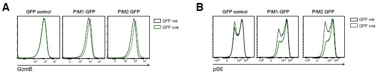
Other experiments could also look at how PIM1/2 KO influences the differentiation of T cell populations/states during ex vivo stimulation of PBMCs or in vivo infection models using (high-dimensional) flow cytometry (rather than using bulk proteomics/RNA seq which only provide an overview of all cells combined).
We did consider the idea of in vivo experiments with the Pim1/2 dKO mice but rejected this idea as the mice have lost PIM kinases in all tissues and so we would not be able to understand if any phenotype was CD8 T cell selective. To note the Pim1/2 dKO mice are smaller than normal wild type mice (discussed further below) and clearly have complex phenotypes. An ideal experiment would be to make mice with floxed Pim1 and Pim2 alleles so that one could use cre recombinase to make a T cell-specific deletion and then study the impact of this in in vivo models. We did not have the budget or ethical approval to make these mice. Moreover, this study was carried out during the COVID pandemic when all animal experiments in the UK were severely restricted. So our objective was to get a molecular understanding of the consequences of losing theses kinases for CD8 T cells focusing on using controlled in vitro systems. We felt that this would generate important data that would guide any subsequent experiments by other groups interested in these enzymes.
We do accept the comment about bulk population proteomics. Unfortunately, single cell proteomics is still not an option at this point in time. High resolution multidimensional flow cytometry is a valuable technique but is limited to looking at only a few proteins for which good antibodies exist compared to the data one gets with high resolution proteomics.
Alongside this, performing a PCA of bulk RNA seq/proteomes or Untreated vs. IL-2 vs. IL-15 of WT and PIM1/2 knockout T cells would help cement their argument in the discussion about PIM1/2 knockout cells being distinct from a memory phenotype.
We thank the reviewer for this very good suggestion. We have now included PCAs for the RNAseq and proteomics datasets of IL-2 and IL-15 expanded WT vs Pim dKO CTL in Fig S5 and added the following text to the discussion section of the manuscript (lines 429-431):
“… and PCA plots of IL-15 and IL-2 proteomics and RNAseq data show that Pim dKO IL-2 expanded CTL are still much more similar to IL-2 expanded WT CTL than to IL-15 expanded CTL (Fig S5)”.
Recommendations for the authors:
Reviewer #1 (Recommendations For The Authors):
In panel B of Figure S1, are the smaller numbers of splenocytes found in dKO fully accounted for by a reduction in the numbers of T cells or also correspond to a reduction in B cell numbers? Are the thymus and lymph nodes showing the same trend?
We’re happy to clarify on this.
Since we were focused on T cell phenotypes in the paper this is what we have plotted in this figure, however there is also a reduction in total number of B, NK and NKT cells in the Pim dKO mice (see James et al, Nat Commun, 2021 for additional subset percentages). We find that all immune subsets we have measured make up the same % of the spleen in Pim dKO vs WT mice (we show this for T cell subsets in what was formerly Fig S1C and is now Fig S1A), the total splenocyte count is just lower in the Pim dKO mice (which we show in what was formerly Fig S1B and is now Fig S1C). To note, the Pim dKO mice were smaller than their WT counterparts (though we have not formally weighed and quantified this) and we think this is likely the major factor leading to lower total splenocyte numbers.
We have not checked the thymus so can’t comment on this. We can confirm that lymph nodes from Pim dKO mice had the same number and % CD4 and CD8 T cells as in WT.
For our in vitro studies we have made sure to either use co-cultures or for single WT and Pim dKO cultures to equalise starting cell densities between wells to account for the difference in total splenocyte number. We have now clarified this point in the methods section lines 682-684
“For generation of memory-like or effector cytotoxic T lymphocytes (CTL) from mice with polyclonal T cell repertoires, LN or spleen single cell suspensions at an equal density for WT and Pim dKO cultures (~1-3 million live cells/mL)….”
Reviewer #2 (Recommendations For The Authors):
Line 89-99 - PIM kinase expression is elevated in T cells in autoimmunity and inhibiting therefore may make some sense if PIM is enhancing T cell activity. Why then would you use an inhibitor in cancer settings? This needs better clarification for readers, with reference to T cells, particularly given this is an important justification for looking at PIM kinases in T cells.
We thank the reviewer for highlighting the lack of clarity in our explanation here.
PIM kinase inhibitors alone are proposed as anti-tumour therapies for select cancers to block tumour growth. However so far these monotherapies haven’t been very effective in clinical trials and combination treatment options with a number of strategies are being explored. There are two lines of logic for why PIM kinase inhibitors might be a good combination with an e.g. anti-PD1 or adoptive T cell immunotherapy. 1) PIM kinase inhibition has been shown to reduce inhibitory/suppressive surface proteins (e.g. PDL1) and cytokine (e.g. TGFbeta) expression in tumour cells and macrophages in the tumour microenvironment. 2) Inhibiting glycolysis and increasing memory/stem-like phenotype has been identified as desirable for longer-lasting more potent anti-tumour T cell immunity. PIM kinase inhibition has been shown to reduce glycolytic function and increase several ‘stemness’ promoting transcription factors e.g. TCF7 in a previous study. Controlled murine cancer models have shown improvement in clearance with the combination of pan-Pim kinase inhibitors and anti-PD1/PDL1 treatments (Xin et al, Cancer Immunol Res, 2021 and Chatterjee et al, Clin Cancer Res 2019).
It is worth noting, this is seemingly contradictory with other studies of Pim kinases in T cells that have generally found Pim1/2/3 deletion or inhibition in T cells to be suppressive of their function.
We have clarified this reasoning/seeming conflict of results in the introductory text as follows (lines 90-101):
“PIM kinase inhibitors have also entered clinical trials to treat some cancers (e.g. multiple myeloma, acute myeloid leukaemia, prostate cancer), and although they have not been effective as a monotherapy, there is interest in combining these with immunotherapies. This is due to studies showing PIM inhibition reducing expression of inhibitory molecules (e.g. PD-L1) on tumour cells and macrophages in the tumour microenvironment and a reported increase of stem-like properties in PIM-deficient T cells which could potentially drive longer lasting anti-cancer responses (Chatterjee et al., 2019; Xin et al., 2021; Clements and Warfel, 2022). However, PIM kinase inhibition has also generally been shown to be inhibitory for T cell activation, proliferation and effector activities (Fox et al., 2003; Mikkers et al., 2004; Jackson et al., 2021) and use of PIM kinase inhibitors could have the side effect of diminishing the anti-tumour T cell response.”
Line 93 - The use of 'some cancers' is rather vague and unscientific - please correct phrasing like this. The same goes for lines 54 and 77 (some kinases and some analyses).
We have clarified the sentence in what is now Line 91 to include examples of some of the cancers that PIM kinase inhibitors have been explored for (see text correction in response to previous reviewer comment), which are predominantly haematological malignancies. The use of the phrase ‘some kinases’ and ‘some analyses’ in what are now Lines 52 and 75 is in our view appropriate as the subsequent sentence/(s) provide specific details on the kinases and analyses that are being referred to.
Lines 146-147 - Could it be that rather than redundancies, PIM KO is simply not influential on TCR/CD28 signalling in general but influences other pathways in the T cell?
We agree that the lack of PIM1/2 effect could also be because PIM targets downstream of TCR/CD28 are not influential and have clarified the text as follows (lines 156-161):
“These experiments quantified expression of >7000 proteins but found no substantial quantitative or qualitative differences in protein content or proteome composition in activated WT versus Pim dKO CD4 and CD8 T cells (Fig 1G-H) (Table S1). Collectively these results indicate that PIM kinases do not play an important unique role in the signalling pathways used by the TCR and CD28 to control T cell activation.”
Line 169 - Instead of specifying control - maybe put upregulate or downregulate for clarity.
We have changed the text as per reviewer suggestion (see line 183)
Line 182-183 - I would move the call out for Figure 2D to after the last call out for Figure 2C to make it more coherent for readers.
We have changed the text as per reviewer suggestion (see lines 197-200)
Line 190 - 14,000 RNA? total, unique? mRNA?
These are predominantly mRNA since a polyA enrichment was performed as part of the standard TruSeq stranded mRNA sample preparation process, however, a small number of lncRNA etc were also detected in our RNA sequencing. We left the results in as part of the overall analysis since it may be of interest to others but don’t look into it further. We do mention the existence of the non-mRNA briefly in the subsequent sentence when discussing the total number of DE RNA that were classified as protein coding vs non-coding.
We have edited this sentence as follows to more accurately reflect that the RNA being referred to is polyA+ (lines 205-207):
“The RNAseq analysis quantified ~14,000 unique polyA+ mRNA and using a cut off of >1.5 fold-change and q-value <0.05 we saw that the abundance of 381 polyA+ RNA was modified by Pim1/Pim2-deficiency (Fig 2E) (Table S2A).
Questions/points regarding figures:
Figure 1 - Is PIM3 changed in expression with the knockout of PIM1/2 in mice? Although the RNA is low could there be some compensation here? The authors put a good amount of effort in to showing that mouse T cells do not exhibit differences from knocking out pim1/2 i.e., Efforts have been made to address this using activation markers and cell size, cytokines, and proliferation and proteomics of activated T cells. What do the resting T cells look like though? Although TCR signalling is not impacted, other pathways might be. Resting-state comparison may identify this.
In all experiments Pim3 mRNA was only detected at very low levels and no PIM3 protein was detected by mass spectrometry in either wild type or PIM1/2 double KO TCR activated or cytokine expanded CD8 T cells (See Tables S1, S3, S4). There was similarly no change in Pim3 mRNA expression in RNAseq of IL-2 or IL-15 expanded CD8 T cells (See Tables S2, S6). While we have not confirmed this in resting state cells for all the conditions examined, there is no evidence that PIM3 compensates for PIM1/2deficiency or that PIM3 is substantially expressed in T cells.
Figure 1A&B - Does PIM kinase stay elevated when removing TCR stimulus? During egress from lymph node and trafficking to infection/tumour/autoimmune site, T cells experience a period of 'rest' from T-cell activation so is PIM upregulation stabilized, or does it just coincide with activation? This could be a crucial control given the rest of the study focuses on day 6 after initial activation (which includes 4 days of 'rest' from TCR stimulation). Nice resolution on early time course though.
This is an interesting question. Unfortunately, we do not know how sensitive PIM kinases are to TCR stimulus withdrawal, as we have not tried removing the TCR stimulus during early activation and measuring PIM expression.
Based on the data in Fig 2A there is a hint that 4 hours withdrawal of peptide stimulus may be enough to lose PIM1/2 expression (after ~36 hrs of TCR activation), however, we did not include a control condition where peptide is retained within the culture. Therefore, we cannot resolve this question from the current experimental data, as this difference could also be due to a further increase in PIMs in the cytokine treated conditions rather than a reduction in expression in the no cytokine condition. This ~36-hour time point is also at a stage where T cells have become more dependent on cytokines for their sustained signalling compared to TCR stimulus.
It is worth noting that PIM kinases are thought to have fairly short mRNA and protein half lives (~5-20 min for PIM1 in primary cells, ~10 min – 1 hr for PIM2). This is consistent with previous observations that cytotoxic T cells need sustained IL-2/Jak signalling to sustain PIM kinase expression, e.g. in Rollings et al (2018) Sci Signaling, DOI:10.1126/scisignal.aap8112 . We would therefore expect that sustained signalling from some external signalling receptor whether this is TCR, costimulatory receptors or cytokines is required to drive Pim1/2 mRNA and protein expression.
Figure 1D - the CD4 WT and Pim dKO plots are identical - presumably a copying error - please correct.
We apologise for the copying error and have amended the manuscript to show the correct data. We thank the reviewer for noticing this mistake.
In Figure 1H - there is one protein found significant - would be nice to mention what this is - for example, if this is a protein that influences TCR levels this could be quite important.
The protein is Phosphoribosyl Pyrophosphate synthase 1 like 1 (Prps1l1).
This was a low confidence quantification (based on only 2 peptides) with no known function in T cells. Based on what is known, this gene is predominantly expressed in the testis (though also detected in spleen, lung, liver). A whole-body KO mouse found no difference in male fertility. No further phenotype has been reported in this mouse. See: Wang et al (2018) Mol Reprod Dev, DOI: 10.1002/mrd.23053
We have added the following text to the legend of Figure 1H to address this protein:
“Phosphoribosyl Pyrophosphate synthase 1 like 1 (Prps1l1), was found to be higher in Pim dKO CD8 T cells, but was a low confidence quantification (based on only 2 unique peptides) with no known function in T cells.”
Figure S1 - In your mouse model the reduction in CD4 T cells is quite dramatic in the spleen - is this reduced homing or reduced production of T cells through development?
Could you quantify the percentage of CD45+ cells that are T cells from blood too? Would be good to have a more thorough analysis of this new mouse model.
We apologise for the lack of clarity around the Pim dKO mouse phenotype. Something we didn’t mention previously due to a lack of a formal measurement is that the Pim dKO mice were typically smaller than their WT counterparts. This is likely the main reason for total splenocytes being lower in the Pim dKO mice - every organ is smaller. It is not a phenotype reported in Pim1/2 dKO mice on an FVB background, though has been reported in the Pim1/2/3 triple KO mouse before (see Mikkers et al, Mol Cell Biol 2004 doi: 10.1128/MCB.24.13.6104-6115.2004).
The % cell type composition of the spleen is equivalent between WT and Pim dKO mice and as mentioned above, was controlled for when setting up of our in vitro cultures.
We have revised the main text and changed the order of the panels in Fig S1 to make this caveat clearer as follows (lines 138-144):
“There were normal proportions of peripheral T cells in spleens of Pim dKO mice (Fig S1A) similar to what has been reported previously in Pim dKO mice on an FVB/N genetic background (Mikkers et al., 2004), though the total number of T cells and splenocytes was lower than in age/sex matched wild-type (WT) mouse spleens (Fig S1B-C). This was not attributable to any one cell type (Fig S1A)(James et al., 2021) but was instead likely the result of these mice being smaller in size, a phenotype that has previously been reported in Pim1/2/3 triple KO mice (Mikkers et al., 2004).”
Figure S1C - why are only 10-15% of the cells alive? Please refer to this experiment in the main text if you are going to include it in the supplementary figure.
With regards what was previously Fig S1C (now Fig S1A) we apologise for our confusing labelling. We were quoting these numbers as the percentage of live splenocytes (i.e. % of live cells). Typically ~80-90% of the total splenocytes were alive by the time we had processed, stained and analysed them by flow cytometry direct ex vivo. Of these CD4 and CD8 T cells made up ~%10-15 of the total live splenocytes (with most of the rest of the live cells being B cells).
We have modified the axis to say “% of splenocytes” to make it clearer that this is what we are plotting.
Figure S1 - Would be good to show that the T cells are truly deficient in PIM1/2 in your mice to be absolutely sure. You could just make a supplementary plot from your mass spec data.
This is a good suggestion and we have now included this data as supplementary figure 2.
To note, due to the Pim1 knockout mouse design this is not as simple as showing presence or absence of total PIM1 protein detection in this instance.
To elaborate: the Pim1/Pim2 whole body KO mice used in this study were originally made by Prof Anton Berns’ lab (Pim1 KO = Laird et al Nucleic Acids Res, 1993, doi: 10.1093/nar/21.20.4750, with more detail on deletion construct in te Riele, H. et al, Nature,1990, DOI: 10.1038/348649a0; Pim2 KO = Mikkers et al, Mol Cell Biol, 2004, DOI: 10.1128/MCB.24.13.6104-6115.2004). They were given to Prof Victor Tybulewicz on an FVB/N background. He then backcrossed them onto the C57BL/6 background for > 10 generations then gave them to us to intercross into Pim1/2 dKO mice on a C57BL/6 background.
The strategy for Pim1 deletion was as follows:
A neomycin cassette was recombined into the Pim1 gene in exon 4 deleting 296 Pim1 nucleotides. More specifically, the 98th pim-1 codon (counted from the ATG start site = the translational starting point for the 34 kDa isoform of PIM1) was fused in frame by two extra codons (Ser, Leu) to the 5th neo codon (pKM109-90 was used). The 3'-end of neo included a polyadenylation signal. The cassette also contains the PyF101 enhancer (from piiMo +PyF101) to ensure expression of neo on homologous recombination in ES cells.
Collectively this means that the PIM1 polypeptide is made prior to amino acid 98 of the 34 kDa isoform but not after this point. This deletes functional kinase activity in both the 34 kDa and 44 kDa PIM1 isoforms. Ablation of PIM1 kinase function using this KO was verified via kinase activity assay in Laird et al. Nucelic Acids Res 1993.
The strategy to delete Pim2 was as follows:
“For the Pim2 targeting construct, genomic BamHI fragments encompassing Pim2 exons 1, 2, and 3 were replaced with the hygromycin resistance gene (Pgp) controlled by the human PGK promoter.” (Mikkers et al Mol Cell Biol, 2004)
The DDA mass spectrometry data collected in Fig 1 G-H and supplementary table 1 confirmed we do not detect peptides from after amino acid residue 98 in PIM1 (though we do detect peptides prior to this deletion point) and we do not detect peptides from the PIM2 protein in the Pim dKO mice. Thus confirming that no catalytically active PIM1/PIM2 proteins were made in these mice.
We have added a supplementary figure S2 showing this and the following text (Lines 155-156):
“Proteomics analysis confirmed that no catalytically active PIM1 and PIM2 protein were made in Pim dKO mice (Fig S2).”
Figure 2A - I found the multiple arrows a little confusing - would just use arrows to indicate predicted MW of protein and stars to indicate non-specific. Why are there 3 bands/arrows for PIM2?
The arrows have now been removed. We now mention the PIM1 and PIM2 isoform sizes in the figure legend and have left the ladder markings on the blots to give an indication of protein sizes. There are 2 isoforms for PIM1 (34 and 44 kDa) in addition to the nonspecific band and 3 isoforms of PIM2 (40, 37, 34 kDa, though two of these isoform bands are fairly faint in this instance). These are all created via ribosome use of different translational start sites from a single Pim1 or Pim2 mRNA transcript.
The following text has been added to the legend of Fig 2A:
“Western blots of PIM1 (two isoforms of 44 and 34 kDa, non-specific band indicated by *), PIM2 (three isoforms of 40, 37 and 34 kDa) or pSTAT5 Y694 expression.”
Figure 2A - why are the bands so faint for PIM1/2 (almost non-existent for PIM2 under no cytokine stim) here yet the protein expression seems abundant in Figure 1B upon stim without cytokines? Is this a sensitivity issue with WB vs proteomics? My apologies if I have missed something in the methods but please explain this discrepancy if not.
There is differing sensitivity of western blotting versus proteomics, but this is not the reason for the discrepancy between the data in Fig 1B versus 2A. These differences reflect that Fig1 B and Fig 2A contrast PIM levels in two different sets of conditions and that while proteomics allows for an estimate of ‘absolute abundance’ Western blotting only shows relative expression between the conditions assessed.
To expand on this… Fig 1B proteomics looks at naïve versus 24 hr aCD3/aCD28 TCR activated T cells. The western blot data in Fig 2A looks at T cells activated for 1.5 days with SIINFEKL peptide and then washed free of the media containing the TCR stimulus and cultured with no stimulus for 4 or 24 hrs hours and contrast this with cells cultured with IL-2 or IL-15 for 4 or 24 hours. All Fig 2A can tell us is that cytokine stimuli increases and/or sustains PIM1 and PIM2 protein above the level seen in TCR activated cells which have not been cultured with cytokine for a given time period. Overexposure of the blot does reveal detectable PIM1 and PIM2 protein in the no cytokine condition after 4 hrs. Whether this is equivalent to the PIM level in the 24 hr TCR activated cells in Fig 1B is not resolvable from this experiment as we have not included a sample from a naïve or 24 hr TCR activated T cell to act as a point of reference.
Figure 4F - Your proteomics data shows substantial downregulation in proteomics data for granzymes and ifny- possibly from normalization to maximise the differences in the graph - and yet your flow suggests there are only modest differences. Can you explain why a discrepancy in proteomics and flow data - perhaps presenting in a more representative manner (e.g., protein counts)?
The heatmaps are a scaled for ‘row max’ to ‘row min’ copy number comparison on a linear scale and do indeed visually maximise differences in expression between conditions. This feature of these heatmaps is also what makes the lack of difference in GzmB and GzmA at the mRNA heatmap in Fig 5C quite notable.
We have now included bar graphs of Granzymes A and B and IFNg protein copy number in Figure 4 (see new Fig 4G-H) to make clearer the magnitude of the effect on the major effector proteins involved in CTL killing function. It is worth noting that flow cytometry histograms from what was formerly Fig 4G (now Fig 4I) are on a log-scale so the shift in fluorescence does generally correspond well with the ~1.7-2.75-fold reduction in protein expression observed.
Figure 4G - did you use isotype controls for this flow experiment? Would help convince labelling has worked - particularly for low levels of IFNy production.
We did not use isotype controls in these experiments but we are using a well validated interferon gamma antibody and very carefully colour panel/compensation controls to minimise background staining. The only ways to be 100% confident that an antibody is selective is to use an interferon gamma null T cell which we do not have. We do however know that the antibody we use gives flow cytometry data consistent with other orthogonal approaches to measure interferon gamma e.g. ELISA and mass spectrometry.
Figure 5M - why perform this with just the PIM kinase inhibitors? Can you do this readout for the WT vs. PIM1/2KO cells too? This would really support your claims for the paper about PIM influencing translation given the off-target effects of SMIs.
Regrettably we have not done this particular experiment with the Pim dKO T cells. As mentioned above, due to this work being performed predominantly during the COVID19 pandemic we ultimately had to make the difficult decision to cease colony maintenance. When work restrictions were lifted we could not ethically or economically justify resurrecting a mouse colony for what was effectively one experiment, which is why we chose to test this key biological question with small molecule inhibitors instead.
We appreciate that SMIs have off target effects and this is why we used multiple panPIM kinase inhibitors for our SMI validation experiments. While the use of 2 different inhibitors still doesn’t completely negate the concern about possible off-target effects, our conclusions re: PIM kinases and impact on proteins synthesis are not solely based on the inhibitor work but also based on the decreased protein content of the PIM1/2 dKO T cells in the IL-2 CTL, and the data quantifying reductions in levels of many proteins but not their coding mRNA in PIM1/2dKO T cells compared to controls.
-
-
www.biorxiv.org www.biorxiv.org
-
Author response:
The following is the authors’ response to the original reviews
Reviewer #1:
Comment 0: Summary: This work presents an Interpretable protein-DNA Energy Associative (IDEA) model for predicting binding sites and affinities of DNA-binding proteins. Experimental results demonstrate that such an energy model can predict DNA recognition sites and their binding strengths across various protein families and can capture the absolute protein-DNA binding free energies.
We appreciate the reviewer’s careful assessment of the paper, and we thank the reviewer for the insightful suggestions and comments.
Comment 1: Strengths: (1) The IDEA model integrates both structural and sequence information, although such an integration is not completely original. (2) The IDEA predictions seem to have agreement with experimental data such as ChIP-seq measurements.
We appreciate the reviewer’s positive comments on the strength of the paper.
Comment 2: Weaknesses: (1) The authors claim that the binding free energy calculated by IDEA, trained using one MAX-DNA complex, correlates well with experimentally measured MAX-DNA binding free energy (Figure 2) based on the reported Pearson Correlation of 0.67. However, the scatter plot in Figure 2A exhibits distinct clustering of the points and thus the linear fit to the data (red line) may not be ideal. As such. the use of the Pearson correlation coefficient that measures linear correlation between two sets of data may not be appropriate and may provide misleading results for non-linear relationships.
We thank the reviewer for the insightful comments and agree that a linear fit between our predictions and the experimental data may not be the best measure of performance. The primary utility of the IDEA model is to predict high-affinity DNA-binding sequences for a given DNA-binding protein by assessing the relative binding affinities across different DNA sequences. In this regard, the ranked order of predicted sequence binding affinities serves as a better metric for evaluating the success of this model. To evaluate this, we calculated both Spearman’s rank correlation coefficient, which does not rely on linear correlation, and the Pearson correlation coefficient between our predictions and the experimental results. As shown in Figure 2, our computation shows a Spearman’s rank correlation coefficient of 0.65 for the MAX-based predictions using one MAX-DNA complex (PDB ID: 1HLO), supporting the model’s capability to effectively distinguish strong from weak binders.
Although our model generally captures the relative binding affinities across different DNA sequences, its predictive accuracy diminishes for low-affinity sequences (Figure 2).
This could be due to two limitations of the current modeling framework: (1) The model is residue-based and estimates binding free energy as the additive sum of contributions from individual contacting amino-acid-nucleotide pairs. This assumption does not account for cooperative effects caused by simultaneous changes at multiple nucleotide positions. One potential direction to further improve the model would be to use a finergrained representation by incorporating more atom types within contacting residues, and to use a many-body potential to better capture cooperative effects from multiple mutations. (2) The model assumes that the target DNA adopts the same binding interface as in the reference crystal structure. However, sequence-dependent DNA shape has been shown to be important in determining protein-DNA binding affinity [1]. To address this limitation, a future direction is to use deep-learning-based methods to incorporate predicted DNA shape or protein-DNA complex structures based on their sequences [2, 3] into our model prediction.
To fully evaluate the predictive power of IDEA, we have included Spearman’s rank correlation coefficient for every correlation plot in this manuscript and have updated the relevant texts. Across all our analyses, the Spearman’s rank correlation coefficients reveal similar predictive performance as the Pearson correlation coefficients. Additionally, we have included in our discussion the current limitations of our model and potential directions for future improvement.
We have edited our Discussion Section to include a discussion on the limitations of the current model. Specifically, the added texts are:
“Although IDEA has proved successful in many examples, it can be improved in several aspects. The model currently assumes the training and testing sequences share the same protein-DNA structure. While double-stranded DNA is generally rigid, recent studies have shown that sequence-dependent DNA shape contributes to their binding specificity [1, 2, 4]. To improve predictive accuracy, one could incorporate predicted DNA shapes or structures into the IDEA training protocol. In addition, the model is residue-based and evaluates the binding free energy as the additive sum of contributions from individual amino-acid-nucleotide contacts. This assumption does not account for cooperative effects that may arise from multiple nucleotide changes. A potential refinement could utilize a finer-grained model that includes more atom types within contacting residues and employs a many-body potential to account for such cooperative effects.”
Comment 3: (2) In the same vein, the linear Pearson Correlation analysis performed in Figure 5A and the conclusion drawn may be misleading.
We thank the reviewer for the insightful comments. As noted in our response to the previous comment, we have added Spearman’s rank correlation coefficient in addition to the Pearson correlation coefficient to all correlation plots, including Figure 5A.
Comment 4: (3) The authors included the sequences of the protein and DNA residues that form close contacts in the structure in the training dataset, whereas a series of synthetic decoy sequences were generated by randomizing the contacting residues in both the protein and DNA sequences. In particular, synthetic decoy binders were generated by randomizing either the DNA (1000 sequences) or protein sequences (10,000 sequences) from the strong binders. However, the justification for such randomization and how it might impact the model’s generalizability and transferability remain unclear.
We thank the reviewer for the insightful comments. The number of randomizing sequences was chosen to strike a balance between sufficient sequence coverage and computational feasibility. Because proteins have more types of amino acids than four nucleotides in DNA, we utilized more protein decoy sequences than DNA decoys. To examine the robustness of our choice against different number of decoy sequences, we repeated the transferability analysis within the bHLH superfamily (Figure 3A) and the generalizability analysis across 12 protein families (Figure 2E) using two additional decoy sequence combinations: (1) 1000 DNA sequences and 1000 protein sequences; (2) 100 DNA sequences and 1000 protein sequences. As shown in Figure S15, we achieved similar results to those reported using the original decoy set, demonstrating the robustness of our model prediction against the variations in the number of decoys. We have included this figure as Figure S15.
Comment 5: (4) The authors performed Receiver Operating Characteristic (ROC) analysis and reported the Area Under the Curve (AUC) scores in order to quantitate the successful identification of the strong binders by IDEA. It would be beneficial to analyze the precision-recall (PR) curve and report the PRAUC metric which could be more robust.
We agree with the reviewer that more robust statistical metrics should be used to evaluate our model’s performance. We have included the PRAUC score as an additional evaluation metric of the model’s performance. Due to a significant imbalance in the number of strong and weak binders from the experimental data [5], where the experimentally identified strong binders are far fewer than the weak binders, we reweighted the sample to achieve a balanced evaluation [6], using 0.5 as the baseline for randomized prediction. As shown in Figure S5, IDEA achieves successful predictions in 18 out of 22 cases, demonstrating its predictive accuracy.
The updated PRAUC result has been included as Figure S5 in the manuscript. We have also included the detailed precision-recall curves for each case in Figure S4.
In addition, we have provided PRAUC scores for comparing the performance of IDEA with other models, and have summarized these results in Table S2.
Reviewer #2:
Comment 0: Summary: Zhang et al. present a methodology to model protein-DNA interactions via learning an optimizable energy model, taking into account a representative bound structure for the system and binding data. The methodology is sound and interesting. They apply this model for predicting binding affinity data and binding sites in vivo. However, the manuscript lacks discussion of/comparison with state-of-the-art and evidence of broad applicability. The interpretability aspect is weak, yet over-emphasized.
We appreciate the reviewer’s excellent summary of the paper, and we thank the reviewer for the insightful suggestions and comments.
Comment 1: Strengths: The manuscript is well organized with good visualizations and is easy to follow. The methodology is discussed in detail. The IDEA energy model seems like an interesting way to study a protein-DNA system in the context of a given structure and binding data. The authors show that an IDEA model trained on one system can be transferred to other structurally similar systems. The authors show good performance in discriminating between binding-vs-decoy sequences for various systems, and binding affinity prediction. The authors also show evidence of the ability to predict genome-wide binding sites.
We appreciate the reviewer’s strong assessment of the strengths of this paper. We have further refined our Methods Section to ensure all modeling details are clearly presented.
Comment 2: Weaknesses: An energy-based model that needs to be optimized for specific systems is inherently an uncomfortable idea. Is this kind of energy model superior to something like Rosetta-based energy models, which are generally applicable? Or is it superior to family-specific knowledge-based models? It is not clear.
We thank the reviewer for the insightful comments. The protein-DNA energy model facilitates the calculation of protein-DNA binding free energy based on protein-DNA structures and sequences. Because this model is optimized using the structure-sequence relationship of given protein-DNA complexes, it features specificity based on the conserved structural interface characteristic of each protein family. Because of that, its predictive accuracy depends on the degree of protein-DNA interface similarity between the training and target protein-DNA pairs, and is distinct from a general protein-DNA energy model, such as a Rosetta-based energy model. The model has some connections to the familyspecific energy model. As shown in Author response image 1, systems belonging to the same protein superfamily (MAX and PHO4) exhibit similar patterns in their learned energy models, in contrast to those from a different superfamily (PDX1).
Author response image 1:
Comparison of learned energy models for different protein-DNA complexes: MAX (A), PHO4 (B), and PDX1 (C). MAX and PHO4 are members of the Helixloop-helix (HLH) CATH protein superfamily (4.10.280.100), while PDX1 belongs to another Homeodomain-like CATH protein superfamily (1.10.10.60).
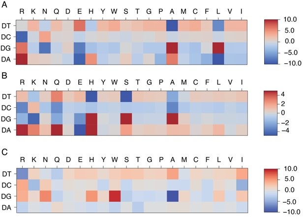
To compare our approach with both general and family-specific knowledge-based energy models, we conducted two studies. First, we incorporated a knowledge-based generic protein-DNA energy model (DBD-Hunter) learned from the protein-DNA database, reported by Skoinick and coworkers [7], into our prediction protocol. This model assigns interaction energies to different functional groups within each DNA nucleotide (e.g., phosphate (PP), sugar (SU), pyrimidine (PY), and imidazole (IM) groups). For our comparison, we averaged the energy contributions of these groups within each nucleotide and replaced the IDEA-learned energy model with this generic one to test its ability to differentiate strong binders from weak binders in the HT-SELEX dataset [5]. As shown in Figure S6, the IDEA model generally achieves better performance than the generic energy model.
Additionally, we compared IDEA with rCLAMPS, a family-specific energy model developed to predict protein-DNA binding specificity in the C2H2 and homeodomain families.
As shown in Table S1 and Table S2, IDEA also shows better performance than rCLAMPS in most cases across the C2H2 and homeodomain families, demonstrating that it has better predictive accuracy than both state-of-the-art family-specific and generic knowledgebased models.
We have included relevant texts in Appendix Section Comparison of IDEA predictive performance Using HT-SELEX data to clarify this point. The added texts are:
In addition, we compared the performance of IDEA with both general and family-specific knowledge-based energy models. First, we incorporated a knowledgebased generic protein-DNA energy model (DBD-Hunter) learned from the protein-DNA database, reported by Skoinick and coworkers [7], into our prediction protocol. This model assigns interaction energies to different functional groups within each DNA nucleotide, including phosphate (PP), sugar (SU), pyrimidine (PY), and imidazole (IM) groups. For our comparison, we averaged the energy contributions of these groups within each nucleotide and replaced the IDEA-learned energy model with the DBD-Hunter model to assess its ability to differentiate strong binders from weak binders in the HTSELEX dataset [5]. Additionally, we compared IDEA with rCLAMPS, a familyspecific energy model developed to predict protein-DNA binding specificity in the C2H2 and homeodomain families. rCLAMPS learns a position-dependent amino-acid-nucleotide interaction energy model. To incorporate this model into the binding free energy calculation, we averaged the energy contributions across all occurrences of each amino-acid-nucleotide pair, which resulted in a 20-by-4 residue-type-specific energy matrix. This matrix is structurally analogous to the IDEA-trained energy model and can be directly integrated into the binding free energy calculations. As shown in Figure S6, Table S1, and Table S2, the IDEA model generally outperforms DBD-Hunter and rCLAMPS, demonstrating that it can achieve better predictive accuracy than both generic and family-specific knowledge-based models.
Comment 3: Prediction of binding affinity is a well-studied domain and many competitors exist, some of which are well-used. However, no quantitative comparison to such methods is presented. To understand the scope of the presented method, IDEA, the authors should discuss/compare with such methods (e.g. PMID 35606422).
We thank the reviewer for the insightful comments. As detailed in our response to Comment 5, we previously misused the term “binding specificity”, and would like to clarify that our model is designed to predict protein-DNA binding affinity. To compare the performance of IDEA with state-of-the-art protein-DNA predictive models, we examined the predictive accuracies of two additional popular computational models: ProBound [8] and DeepBind [9]. ProBound has been shown to have a better performance than several earlier predictive protein-DNA models, including JASPAR 2018 [11], HOCOMOCO [12], Jolma et al. [13], and DeepSELEX [14]. To benchmark these models’ performance, we examine each method’s capability to identify strong binders with the HT-SELEX datasets covering 22 proteins from 12 protein families [5]. As suggested by Reviewer 1, we also calculated the PRAUC score, reweighted to account for data imbalance [6], as a complementary metric for evaluating the model performance.
As shown in Figure S6, Table S1, and Table S2, IDEA ranked second among the three predictive methods. It is important to note that both ProBound and DeepBind were trained on a curated version of the HT-SELEX data [13], which overlaps with the testing data [5]. Compared with them, IDEA was trained only on the given structural and sequence information from a single protein-DNA complex, thus independent of the testing data. In order to assess how IDEA performs when incorporating knowledge from HT-SELEX data, we augmented the training by randomly including half of the HT-SELEX data (see the Methods Section Enhanced Modeling Prediction with SELEX Data). The augmented IDEA model achieved the best performance among all the models. Overall, IDEA can be used to predict protein-DNA affinities in the absence of known binding sequence data, thereby filling a critical gap when such experimental datasets are unavailable.
Additionally, we have conducted a 10-fold cross-validation using the same HT-SELEX data [5] and found that IDEA outperformed a recent regression model that considers the shape of DNA with different sequences [5].
We have revised our text to include the comparison between IDEA and other predictive models. Specifically, we revised the text in Section: IDEA Generalizes across Various Protein Families.
The revised text reads:
“To examine IDEA’s predictive accuracy across different DNA-binding protein families, we applied it to calculate protein-DNA binding affinities using a comprehensive HT-SELEX dataset [5]. We focused on evaluating the capability of IDEA to distinguish strong binders from weak binders for each protein with an experimentally determined structure. We calculated the probability density distribution of the top and bottom binders identified in the SELEX experiment. A well-separated distribution indicates the successful identification of strong binders by IDEA (Figure 2D and S4). Receiver Operating Characteristic (ROC) analysis was performed to calculate the Area Under the Curve (AUC) and the precision-recall curve (PRAUC) scores for these predictions. Further details are provided in the Methods Section Evaluation of IDEA Prediction Using HT-SELEX Data. Our analysis shows that IDEA successfully differentiates strong from weak binders for 80% of the 22 proteins across 12 protein families, achieving AUC and balanced PRAUC scores greater than 0.5 (Figure 2D and S5). To benchmark IDEA’s performance against other leading methods, we compared its predictions with several popular models, including the sequence-based predictive models ProBound [8] and DeepBind [9], the familybased energy model rCLAMPS [10], and the knowledge-based energy model DBD-Hunter [7]. IDEA demonstrates performance comparable to these stateof-the-art approaches, and incorporating sequence features further improves its prediction accuracy (Figure S6, Table S1, and Table S2). We also performed 10-fold cross-validation on the binding affinities of protein–DNA pairs in this dataset and found that IDEA outperforms a recent regression model that considers the shape of DNA with different sequences [5] (Figure S7). Details are provided in Section: Comparison of IDEA predictive performance Using HT-SELEX data.”
We also added one section Comparison of IDEA predictive performance Using HT-SELEX data in the Appendix to fully explain the comparison between IDEA and other popular models. The added texts are:
“To benchmark the performance of IDEA against state-of-the-art protein-DNA predictive models, we evaluated its ability to recognize strong binders with the HT-SELEX datasets across 22 proteins from 12 families [5]. Specifically, we compare IDEA with two widely used sequence-based models: ProBound [8] and DeepBind [9]. ProBound has demonstrated superior performance over many other predictive protein-DNA models, including JASPAR 2018 [11], HOCOMOCO [12], Jolma et al. [13], and DeepSELEX [14]. To use ProBound, we retrieved the trained binding model for each protein from motifcentral.org and used the GitHub implementation of ProBoundTools to infer the binding scores between protein and target DNA sequences. Except for POU3F1, binding models are available for all proteins. Therefore, we excluded POU3F1 and evaluated the protein-DNA binding affinities for the remaining 21 proteins. To use DeepBind, sequence-specific binding affinities were predicted directly with its web server. The Area Under the Curve (AUC) and the Precision-Recall AUC (PRAUC) scores were used as metrics for comparison. An AUC score of 1.0 indicates a perfect separation between the strong- and weak-binder distributions, while an AUC score of 0.5 indicates no separation. Because there is a significant imbalance in the number of strong and weak binders from the experimental data [5], where the strong binders are far fewer than the weak binders, we reweighted the samples to achieve a balanced evaluation, using 0.5 as the baseline for randomized prediction [6]. As summarized in Figure S6, Table S1, and Table S2, IDEA ranked second among the three predictive models. In order to assess the performance of IDEA when augmented with additional protein-DNA binding data, we augmented IDEA using randomly selected half of the HT-SELEX data (see the Methods Section Enhanced Modeling Prediction with SELEX Data). The augmented IDEA model achieved the best performance among all the models.”
“We also performed 10-fold cross-validation using the same HT-SELEX datasets, following the protocol described in the Methods Section Enhanced Modeling Prediction with SELEX Data. For each protein, we divided the entire dataset into 10 equal, randomly assigned folds. In each iteration, we used randomly selected 9 of the 10 folds as the training dataset and the remaining fold as the testing dataset. This process was repeated 10 times so that each fold served as the test set once. We then reported the average R2 scores across these iterations to evaluate IDEA’s predictive performance. Our results are compared with the 1mer and 1mer+shape methods from [5], the latest regression model that considers the shape of DNA with different sequences (Figure S7). This comparative analysis shows IDEA achieved higher predictive accuracy than the state-of-the-art sequence-based protein-DNA binding predictors for proteinDNA complexes that have available experimentally resolved structures.”
“Overall, these results demonstrate that IDEA can be used to predict the proteinDNA pairs in the absence of known binding sequence data, thus filling an important gap in protein-DNA predictions when experimental binding sequence data are unavailable.”
Comment 4: The term “interpretable” has been used lavishly in the manuscript while providing little evidence on the matter. The only evidence shown is the family-specific residue-nucleotide interaction/energy matrix and speculations on how these values are biologically sensible. Recent works already present more biophysical, fine-grained, and sometimes family-independent interpretability (e.g. PMID 39103447, 36656856, 38352411, etc.). The authors should put into context the scope of the interpretability of IDEA among such works.
We thank the reviewer for the insightful comment and agree that “interpretability” should be discussed in a relevant context. In our work, interpretability refers to the familyspecific amino-acid-nucleotide interaction energies identified from the model training, which reveal interaction preferences within protein-DNA binding interfaces. As detailed in our response to Comment 6, we performed principal component analysis (PCA) on the learned energy models and observed clustering of learned energy models corresponding to protein families. Therefore, the IDEA-learned energy models can be used as a signature to capture the energetic preferences of amino-acid-nucleotide interactions within a given protein family. This preference can be used to infer preferred sequence binding motifs, similar to those identified by other computational tools [10, 4, 15, 16].
We have revised the text to clarify the “interpretability” as the family-specific aminoacid-nucleotide interactions that govern sequence-dependent protein-DNA binding, and to discuss IDEA’s interoperability within the context of recent works, including those suggested by the reviewers.
We have revised the text in Introduction. The new text reads:
“Here, we introduce the Interpretable protein-DNA Energy Associative (IDEA) model, a predictive model that learns protein-DNA physicochemical interactions by fusing available biophysical structures and their associated sequences into an optimized energy model (Figure 1). We show that the model can be used to accurately predict the sequence-specific DNA binding affinities of DNA-binding proteins and is transferrable across the same protein superfamily. Moreover, the model can be enhanced by incorporating experimental binding data and can be generalized to enable base-pair resolution predictions of genomic DNA-binding sites. Notably, IDEA learns a family-specific interaction matrix that quantifies energetic interactions between each amino acid and nucleotide, allowing for a direct interpretation of the “molecular grammar” governing sequence-specific protein-DNA binding affinities. This interpretable energy model is further integrated into a simulation framework, facilitating mechanistic studies of various biomolecular functions involving protein-DNA dynamics.”
We have revised the text in Results. The new text reads:
“IDEA is a coarse-grained biophysical model at the residue resolution for investigating protein-DNA binding interactions (Figure 1). It integrates both structures and corresponding sequences of known protein-DNA complexes to learn an interpretable energy model based on the interacting amino acids and nucleotides at the protein-DNA binding interface. The model is trained using available protein-DNA complexes curated from existing databases [17, 18].
Unlike existing deep-learning-based protein-DNA binding prediction models, IDEA aims to learn a physicochemical-based energy model that quantitatively characterizes sequence-specific interactions between amino acids and nucleotides, thereby interpreting the “molecular grammar” driving the binding energetics of protein-DNA interactions. The optimized energy model can be used to predict the binding affinity of any given protein-DNA pair based on its structures and sequences. Additionally, it enables the prediction of genomic DNA binding sites by a given protein, such as a transcription factor. Finally, the learned energy model can be incorporated into a simulation framework to study the dynamics of DNA-binding processes, revealing mechanistic insights into various DNA-templated processes. Further details of the optimization protocol are provided in Methods Section Energy Model Optimization.”
The revised text in Section: Discussion now reads:
“Another highlight of IDEA is its ability to present an interpretable, familyspecific amino acid-nucleotide interaction energy model for given proteinDNA complexes. The optimized IDEA energy model can not only predict sequence-specific binding affinities of protein-DNA pairs but also provide a residue-specific interaction matrix that dictates the preferences of amino acidnucleotide interactions within specific protein families (Figure S11). This interpretable energy matrix would facilitate the discovery of sequence binding motifs for target DNA-binding proteins, complementing both sequencebased [24, 16, 25] and structure-based approaches [10, 26, 4, 15]. Additionally, we integrated this physicochemical-based energy model into a simulation framework, thereby improving the characterization of protein-DNA binding dynamics. IDEA-based simulation enables the investigation into dynamic interactions between various proteins and DNA, facilitating molecular-level understanding of the physical mechanisms underlying many DNA-binding processes, such as transcription, epigenetic regulations, and their modulation by sequence variations, such as single-nucleotide polymorphisms (SNPs) [22, 23].”
Comment 5: The manuscript disregards subtle yet important differences in commonly used terminology in the field. For example, the authors use the term ”specificity” and ”affinity” almost interchangeably (for example, the caption for Figure 3A uses ”specificity” although the Methods text describes the prediction as about ”affinity”). If the authors are looking to predict specificity, IDEA needs to be put in the context of the corresponding state-of-the-art (PMID 36123148, 39103447, 38867914, 36124796, etc).
We really appreciate the reviewer for pointing out the conflation of “specificity” and “affinity” in our manuscript. To clarify, the primary function of IDEA is to predict the binding affinities of protein-DNA pairs in a sequence-specific manner. We have revised the text to clarify the distinction between affinity and specificity and acknowledge prior works, including those provided by the reviewers, that focus on predicting protein-DNA binding specificity.
We have revised the Section title IDEA Accurately Predicts Protein-DNA Binding Specificity to IDEA Accurately Predicts Sequence-Specific Protein-DNA Binding Affinity; and ResidueLevel Protein-DNA Energy Model for Predicting Protein-DNA Recognition Specificities to Predictive Protein-DNA Energy Model at Residue Resolution.
We have revised the text in Introduction. The revised text reads:
“Computational methods complement experimental efforts by providing the initial filter for assessing sequence-specific protein-DNA binding affinity. Numerous methods have emerged to enable predictions of binding sites and affinities of DNA-binding proteins [27, 9, 1, 5, 28, 29, 30, 31, 8]. These methods often utilized machine-learning-based training to extract sequence preference information from DNA or protein by utilizing experimental high-throughput (HT) assays [27, 9, 1, 5, 28, 8], which rely on the availability and quality of experimental binding assays. Additionally, many approaches employ deep neural networks [29, 30, 31], which could obscure the interpretation of interaction patterns governing protein-DNA binding specificities. Understanding these patterns, however, is crucial for elucidating the molecular mechanisms underlying various DNA-recognition processes, such as those seen in TFs [32].”
We have revised the text in Section: IDEA Demonstrates Transferability across Proteins in the Same CATH Superfamily.
The revised text reads:
“Since IDEA relies on the sequence-structure relationship of given protein-DNA complexes to reach predictive accuracy, we inquired whether the trained energy model from one protein-DNA complex could be generalized to predict the sequence-specific binding affinities of other complexes. To test this, we assessed the transferability of IDEA predictions across all 11 structurally available protein-DNA complexes within the MAX TF-associated CATH superfamily (CATH ID: 4.10.280.10, Helix-loop-helix DNA-binding domain). We trained IDEA based on each of these 11 complexes and then used the trained model to predict the MAX-based MITOMI binding affinity. Our results show that IDEA generally makes correct predictions of the binding affinity when trained on proteins that are homologous to MAX, with Pearson and Spearman Correlation coefficients larger than 0.5 (Figure 3A and Figure S10).”
We have revised the caption of Figure 3: The revised text reads:
“IDEA prediction shows transferability within the same CATH superfamily. (A) The predicted MAX binding affinity, trained on other protein-DNA complexes within the same protein CATH superfamily, correlates well with experimental measurement. The proteins are ordered by their probability of being homologous to the MAX protein, determined using HHpred [33]. Training with a homologous protein (determined as a hit by HHpred) usually leads to better predictive performance (Pearson Correlation coefficient > 0.5) compared to non-homologous proteins. (B) Structural alignment between 1HLO (white) and 1A0A (blue), two protein-DNA complexes within the same CATH Helix-loop-helix superfamily. The alignment was performed based on the Ebox region of the DNA [34]. (C) The optimized energy model for 1A0A, a protein-DNA complex structure of the transcription factor PHO4 and DNA, with 33.41% probability of being homologous to the MAX protein. The optimized energy model is presented in reduced units, as explained in the Methods Section: Training Protocol.”
We have revised the text in Section Discussion: The revised text now reads:
“The protein-DNA interaction landscape has evolved to facilitate precise targeting of proteins towards their functional binding sites, which underlie essential processes in controlling gene expression. These interaction specifics are determined by physicochemical interactions between amino acids and nucleotides. By integrating sequences and structural data from available proteinDNA complexes into an interaction matrix, we introduce IDEA, a data-driven method that optimizes a system-specific energy model. This model enables high-throughput in silico predictions of protein-DNA binding specificities and can be scaled up to predict genomic binding sites of DNA-binding proteins, such as TFs. IDEA achieves accurate de novo predictions using only proteinDNA complex structures and their associated sequences, but its accuracy can be further enhanced by incorporating available experimental data from other binding assay measurements, such as the SELEX data [35, 36, 37], achieving accuracy comparable or better than state-of-the-art methods (Figures S2 and S7, Table S1 and S2). Despite significant progress in genome-wide sequencing techniques [38, 39, 40, 41], determining sequence-specific binding affinities of DNA-binding biomolecules remains time-consuming and expensive. Therefore, IDEA presents a cost-effective alternative for generating the initial predictions before pursuing further experimental refinement.”
We have revised the text in Discussion to clarify that the acquired binding affinities of target DNA sequences can be used to help existing models to infer specific DNA binding motifs.
The revised text now reads:
Another highlight of IDEA is its ability to present an interpretable, familyspecific amino acid-nucleotide interaction energy model for given proteinDNA complexes. The optimized IDEA energy model can not only predict sequence-specific binding affinities of protein-DNA pairs but also provide a residue-specific interaction matrix that dictates the preferences of amino acidnucleotide interactions within specific protein families (Figure S11). This interpretable energy matrix would facilitate the discovery of sequence binding motifs for target DNA-binding proteins, complementing both sequencebased [24, 16, 25] and structure-based approaches [10, 26, 4, 15]. Additionally, we integrated this physicochemical-based energy model into a simulation framework, thereby improving the characterization of protein-DNA binding dynamics. IDEA-based simulation enables the investigation into dynamic interactions between various proteins and DNA, facilitating molecular-level understanding of the physical mechanisms underlying many DNA-binding processes, such as transcription, epigenetic regulations, and their modulation by sequence variations, such as single-nucleotide polymorphisms (SNPs) [22, 23].
Comment 6: It is not clear how much the learned energy model is dependent on the structural model used for a specific system/family. It would be interesting to see the differences in learned model based on different representative PDB structures used. Similarly, the supplementary figures show a lack of discriminative power for proteins like PDX1 (homeodomain family), POU, etc. Can the authors shed some light on why such different performances?
We thank the reviewer for the insightful comments and agree that the trained energy model should be presented in the context of protein families. To further analyze the dependence of the energy model on protein family, we visualized the trained energy models for 24 proteins, including all proteins from the HT-SELEX dataset as well as PHO4 (PDB ID: 1A0A) and CTCF (PDB ID: 8SSQ), spanning 12 distinct protein families. To quantitatively assess similarities and differences among these energy models, we flattened each normalized energy model into an 80-dimensional vector and performed principal component analysis (PCA). As shown in Author response image 1 and Figure S11, energy models optimized from the same protein family fall within the same cluster, while those from different protein families exhibit distinct patterns. Moreover, the relative distance between energy models in PCA space reflects the degree of transferability. For example, PHO4 (PDB ID: 1A0A) is positioned close to MAX (PDB ID: 1HLO), whereas USF1 (PDB ID: 1AN4) and TCF4 (PDB ID: 6OD3) are farther away. This is consistent with the results shown in Figure 3A, where the energy model trained from PHO4 has better transferability than those from the other two systems.
We also greatly appreciate the reviewer’s suggestion to examine cases where IDEA failed to demonstrate strong discriminative power. When evaluating the model’s ability to distinguish between strong and weak binders, we used the available experimental structure most similar to the protein employed in the HT-SELEX experiments. In some instances, only the structure of the same protein from a different organism is available. For example, the HT-SELEX data for PDX1-DNA used the human PDX1 protein, but no human PDX1–DNA complex structure is available. Therefore, we used the mouse PDX1–DNA complex (PDB ID: 2H1K) for model training. The differences between species may limit the predictive accuracy of the model. A similar limitation applies to POU3F1, where an available mouse complex (PDB ID: 4Y60) was used to predict human protein–DNA interactions. Notably, DeepBind [9], a sequence-based prediction tool, also failed to distinguish strong from weak binders when using the mouse POU3F1 protein (AUC score: 0.457), but this was corrected with the human POU3F1 protein (AUC score: 0.956).
We also examined the remaining cases where IDEA did not show a clear distinction between strong and weak binders: USF1, Egr1, and PROX1. For PROX1, we initially used the structure of a protein-DNA complex (PDB ID: 4Y60) in training. However, upon closer inspection, we discovered that this structure does not include the PROX1 protein, but SOX-18, a different transcription factor. This explains the inaccurate prediction made by IDEA. Since no experimental PROX1-DNA complex structure is currently available, we have removed this case from our HT-SELEX evaluation.
IDEA also fails to fully resolve the binding preference of USF1. A closer examination of the HT-SELEX data reveals a lack of distinction among the sequences, as most sequences, including those with the lowest M-word (binding affinity) scores, contain the DNA-binding E-box sequence CACGTG. Therefore, USF1 represents a challenging example where the experimental data only consists of strong binders with limited variations in binding affinity, which likely results from differences in flanking sequences of the E-box motif.
Egr1 stands as a peculiar example. Whereas IDEA does not effectively distinguish between the strong and weak binders in the current HT-SELEX dataset, its predictions are consistent with other experimental datasets, including binding affinities measured by kMITOMI [42] (Figure S8A, B), preferred binding sequences from protein-binding microarray, an earlier HT-SELEX experiment, and bacterial one-hybrid data [43]. Therefore, further investigation of the current HT-SELEX data is needed to reconcile these differences.
We have included additional text in Section: IDEA Demonstrates Transferability across Proteins in the Same CATH Superfamily to discuss the PCA analysis and the dependence of the model’s transferability on the similarity among the learned energy models.
The revised text now reads:
“The transferability of IDEA within the same CATH superfamily can be understood from the similarities in protein-DNA binding interfaces, which determine similar learned energy models. For example, the PHO4 protein (PDB I”D: 1A0A) shares a highly similar DNA-binding interface with the MAX protein (PDB ID: 1HLO) (Figure 3B), despite sharing only a 33.41% probability of being homologous. Consequently, the energy model derived from the PHO4DNA complex (Figure 3C) exhibits a similar amino-acid-nucleotide interactive pattern as that learned from the MAX-DNA complex (Figure 2B). To further evaluate the similarity between the learned energy models and their connection to protein families, we performed principal component analysis (PCA) on the normalized energy models across 24 proteins from 12 protein families [5]. Our analysis (Figure S11) reveals that most of the energy models from the same protein family fall within the same cluster, while those from different protein families exhibit distinct patterns. Moreover, the relative distance between energy models in PCA space reflects the degree of transferability between them. For example, PHO4 (PDB ID: 1A0A) is positioned close to MAX (PDB ID: 1HLO), whereas USF1 (PDB ID: 1AN4) and TCF4 (PDB ID: 6OD3) are farther away. This is consistent with the results in Figure 3A, where the energy model trained on PHO4 has better transferability than those trained on USF1 or TCF4.”
We have also added an Appendix section titled Analysis of examples where IDEA fails to recognize strong DNA binders to discuss the examples in which IDEA did not perform well:
“We examine IDEA’s capability in identifying strong binders from the HT-SELEX dataset across 12 protein families [5]. The model successfully predicts 18 out of 22 protein-DNA systems, but the performance is reduced in 4 cases. Closer investigations revealed the source of these limitations. In some instances, only the protein from a different organism is available. For example, the PDX1 HT-SELEX data utilized the human PDX1 protein, but no human PDX1–DNA complex structure is available. Therefore, the mouse PDX1–DNA complex structure (PDB ID: 2H1K) was used for model training. Differences between model organisms may reduce predictive accuracy. A similar limitation applies to POU3F1, where an available mouse complex (PDB ID: 4Y60) was used to predict human protein–DNA interactions. Notably, DeepBind [9], a sequence-based prediction tool, also failed to distinguish strong from weak binders when using the mouse POU3F1 protein (AUC score: 0.457), but this was corrected with the human POU3F1 protein (AUC score: 0.956).
IDEA also fails to fully resolve the binding preference of USF1. A closer examination of the HT-SELEX data reveals a lack of distinction among the sequences, as most sequences, including those with the lowest M-word (binding affinity) scores, contain the DNA-binding E-box sequence CACGTG. Therefore, USF1 represents a challenging example where the experimental data only consists of strong binders with limited variations in binding affinity, which likely results from differences in flanking sequences of the E-box motif.
Egr1 stands as a peculiar example. Whereas IDEA does not effectively distinguish between the strong and weak binders in the current HT-SELEX dataset, its predictions are consistent with other experimental datasets, including binding affinities measured by k-MITOMI [42] (Figure S8A, B), preferred binding sequences from protein-binding microarray, an earlier HT-SELEX experiment, and bacterial one-hybrid data [43]. Therefore, further investigation of the current HT-SELEX data is needed to reconcile these differences.”
Comment 7: It is also not clear if IDEA’s prediction for reverse complement sequences is the same for a given sequence. If so, how is this property being modelled? Either this description is lacking or I missed it.
We thank the reviewer for the insightful comments. Given a target protein-DNA sequence, the IDEA protocol substitutes it into a known protein-DNA complex structure to evaluate the binding free energy, which can be converted into binding affinity. IDEA uses sequence identity to determine whether the forward or reverse strand of the DNA should be replaced. Only the strand most similar to the target sequence is substituted. As a result, the model treats reverse-complement sequences differently. As the orientations of test sequences are specified from 5’ to 3’ in all datasets used in this study (e.g., processed MITOMI, HT-SELEX, and ChIP-seq data), this approach ensures that the target sequences are replaced and evaluated correctly. In cases where sequence orientation is not provided (though this was not an issue in this study), we recommend replacing both the forward and reverse strands with the target sequence separately and evaluating the corresponding protein–DNA binding free energies. Since strong binders are likely to dominate the experimental signals, the higher predicted binding affinity, with stronger binding free energies, should be taken as the model’s final prediction.
We have added one section to the Methods Section titled Treatment of Complementary DNA Sequences to clarify these modeling details.
The specific text reads:
To replace the DNA sequence in the protein-DNA complex structure with a target sequence, IDEA uses sequence identity to determine whether the target sequence belongs to the forward or reverse strand of the DNA in the proteinDNA structure. The more similar strand is selected and replaced with the target sequence. As the orientations of test sequences are specified from 5’ to 3’ in all datasets used in this study (e.g., processed MITOMI, HT-SELEX, and ChIP-seq data), this approach ensures that the target sequences are replaced and evaluated correctly. In cases where sequence orientation is not provided (though this was not an issue in this study), we recommend replacing both the forward and reverse strands with the target sequence separately and evaluating the corresponding protein–DNA binding free energies. Since strong binders are likely to dominate the experimental signals, the higher predicted binding affinity, with stronger binding free energy, should be taken as the model’s final prediction.”
“Comment 8: Page 21 line 403, the E-box core should be CACGTG instead of CACGTC.
We apologize for our oversight and have corrected the relevant text.
Comment 9: The citation for DNAproDB is outdated and should be updated (PMID 39494533).
We thank the reviewer for pointing this out and have updated our citation accordingly.
Reviewer #3:
Comment 0: Summary: Protein-DNA interactions and sequence readout represent a challenging and rapidly evolving field of study. Recognizing the complexity of this task, the authors have developed a compact and elegant model. They have applied well-established approaches to address a difficult problem, effectively enhancing the information extracted from sparse contact maps by integrating artificial sequences decoy set and available experimental data. This has resulted in the creation of a practical tool that can be adapted for use with other proteins.
We appreciate the reviewer’s excellent summary of the paper, and we thank the reviewer for the insightful suggestions and comments.
Comment 1: Strengths: (1) The authors integrate sparse information with available experimental data to construct a model whose utility extends beyond the limited set of structures used for training. (2) A comprehensive methods section is included, ensuring that the work can be reproduced. Additionally, the authors have shared their model as a GitHub project, reflecting their commitment to transparency of research.
We appreciate the reviewer’s strong assessment of the strengths of this paper. In addition to sharing our model on GitHub, we have also uploaded the original data and the essential scripts required to reproduce the results presented in the manuscript. We hope this further demonstrates our commitment to transparency and reproducibility.
Comment 2: Weaknesses: (1) The coarse-graining procedure appears artificial, if not confusing, given that full-atom crystal structures provide more detailed information about residue-residue contacts. While the selection procedure for distance threshold values is explained, the overall motivation for adopting this approach remains unclear. Furthermore, since this model is later employed as an empirical potential for molecular modeling, the use of P and C5 atoms raises concerns, as the interactions in 3SPN are modeled between Cα and the nucleic base, represented by its center of mass rather than P or C5 atoms.
We appreciate the reviewer’s insightful comments. The selection of P and C5 atoms was based on different relative positions of protein and DNA across various complex structures, each with distinctive protein-DNA structural interfaces. To illustrate this, we selected two representative structures where our algorithm selected C5 and P atoms, respectively: MAX-DNA (PDB ID: 1HLO) and FOXP3 (PDB ID: 7TDW). As shown in Author response image 2, in the case of 1HLO, more C5 atoms are within the cutoff distance of 10 A from˚ the protein Cα atoms, thus capturing essential contacting interactions. In contrast, 7TDW has more P atoms within this cutoff. Importantly, several P atoms are distributed on the minor groove of the DNA, which were not captured by the C5 atoms. To maximize the inclusion of relevant structural contacts, we employed a filtering scheme that selectively chooses either P or C5 atoms based on their proximity to the protein to enhance the model prediction. We note that while this scheme is helpful, the IDEA predictions remain robust across different atom selections. To assess this robustness, we performed binding affinity predictions using only P atoms on the HT-SELEX dataset across 12 protein families [5]. Our predictions (Author response table 1) show comparable performance to that achieved using our filtering scheme.
Author response image 2.
Comparison between P and C5 atoms in proximity to the protein 3D structures of MAX–DNA (A) and FOXP-DNA (B) complexes, where P atoms (red sphere) and C5 atoms (blue sphere) that are within 10 A of Cα atoms are highlighted.
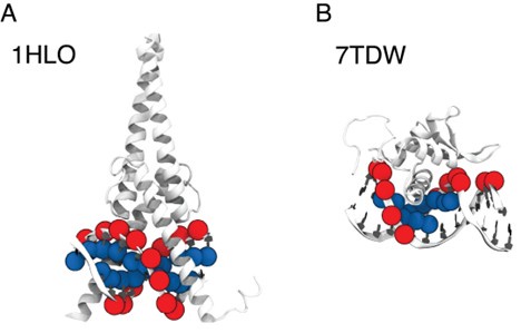
When incorporating the trained IDEA energy model into a simulation model, we acknowledge a potential mismatch between the resolution of the data-driven model (one coarse-grained site per nucleotide) and the 3SPN simulation model (three coarse-grained sites per nucleotide). The selection of nucleic base sites for molecular interactions in the 3SPN model follows our previous work [44] and its associated code implementation. While revisiting this part of the manuscript, we identified an inconsistency in the reported results in Figure 5A of our initial version: Specifically, we previously used the protein side-chain atoms, rather than only the Cα atoms, in model training. Retraining the data using the Cα atoms results in reduced prediction performance for the IDEA model (Figure 5A). Nonetheless, incorporating this updated energy model into simulations still yielded high accuracy in the predicted absolute binding free energies (Author response image 3A), demonstrating the robustness of our simulation framework in predicting absolute binding free energies against variations in atom selection during the IDEA model training. Following the reviewer’s suggestion, we also incorporated the IDEA-trained energy model as short-range van der Waals interactions between protein Cα atoms and DNA P atoms. As shown in Author response image 3B, our simulation reveals a slightly improved performance over our original implementation, with higher Pearson and Spearman correlation coefficients and a fitted slope closer to 1.0. This result suggests that a more consistent atom selection scheme between the data-driven and simulation models can improve the overall predictions. Accordingly, we have updated Figure 5 with this improved setup, using the simulation model with short-range vdW interactions implemented between protein Cα atoms and DNA P atoms (Figure 5C), ensuring consistency between the IDEA model and simulation framework.
Author response table 1.
Comparison of IDEA performance using two DNA atom selection schemes: the filtering scheme presented in the manuscript (C5 and P atoms) versus using only P atoms. Cases where the two schemes result in different atom selections are highlighted in bold.
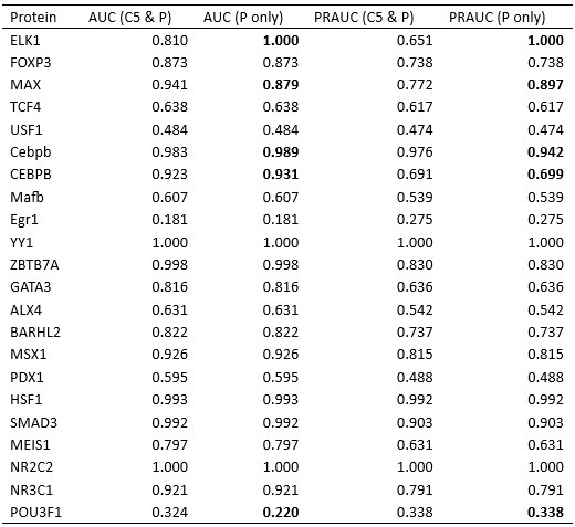
We acknowledge that a gap still exists between the resolution of the data-driven and simulation models. To ensure a completely consistent coarse-grained level between these two models, we will work on implementing the IDEA model output for 1-bead-per-nucleotide DNA simulation models in the future.
Comment 3: (2) Although the authors use a standard set of metrics to assess model quality and predictive power, some ∆∆G predictions compared to MITOMI-derived ∆∆G values appear nonlinear, which casts doubt on the interpretation of the correlation coefficient.
Author response image 3.
Comparison of simulations using different representative atoms (A) Protein-DNA binding simulation with the IDEA-model incorporated as short-range van der Waals between protein Cα atom and nucleic base site. (B) Protein-DNA binding simulation with the IDEA-model incorporated as short-range van der Waals between protein Cα atom and DNA P atoms. The predicted free energies are robust to the choice of DNA representative atoms. The predicted binding free energies are presented in physical units, and error bars represent the standard deviation of the mean.
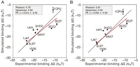
We thank the reviewer for the insightful comments and agree that the linear fit between our model’s prediction and the experimental data may not be the best measure of performance. The primary utility of the IDEA model is to predict high-affinity DNA-binding sequences for a given DNA-binding protein by assessing the relative binding affinities across different DNA sequences. In this regard, the ranked order of predicted sequence binding affinities serves as a better metric for evaluating the success of this model. To evaluate this, we calculated both Spearman’s rank correlation coefficient, which does not rely on linear correlation, and the Pearson correlation coefficient between our predictions and the experimental results. As shown in Figure 2, our computation shows a Spearman’s rank correlation coefficient of 0.65 for the MAX-based predictions using one MAX-DNA complex (PDB ID: 1HLO), supporting the model’s capability to effectively distinguish strong from weak binders.
As reflected in Figure 2 of the main text, although our model generally captures the relative binding affinities across different DNA sequences, its predictive accuracy diminishes for low-affinity sequences (Figure 2). This could be due to two limitations of the current modeling framework: (1) The model is residue-based and estimates binding free energy as the additive sum of contributions from individual contacting amino-acid-nucleotide pairs. This assumption does not account for cooperative effects caused by simultaneous changes at multiple nucleotide positions. One potential direction to further improve the model would be to use a finer-grained representation by incorporating more atom types within contacting residues, and to use a many-body potential to better capture cooperative effects from multiple mutations. (2) The model assumes that the target DNA adopts the same binding interface as in the reference crystal structure. However, sequencedependent DNA shape has been shown to be important in determining protein-DNA binding affinity [1]. To address this limitation, a future direction is to use deep-learningbased methods to incorporate predicted DNA shape or protein-DNA complex structures based on their sequences [2, 3] into our model prediction.
To fully evaluate the predictive power of IDEA, we have included Spearman’s rank correlation coefficient for every correlation plot in this manuscript. Across all our analyses, the Spearman’s rank correlation coefficients reveal similar predictive performance as the Pearson correlation coefficients. Additionally, we have included in our discussion the current limitations of our model and potential directions for future improvement.
We have edited our Discussion Section to include a discussion on the limitations of the current model. Specifically, the added texts are:
“Although IDEA has proved successful in many examples, it can be improved in several aspects. The model currently assumes the training and testing sequences share the same protein-DNA structure. While double-stranded DNA is generally rigid, recent studies have shown that sequence-dependent DNA shape contributes to their binding specificity [1, 2, 4]. To improve predictive accuracy, one could incorporate predicted DNA shapes or structures into the IDEA training protocol. In addition, the model is residue-based and evaluates the binding free energy as the additive sum of contributions from individual amino-acid-nucleotide contacts. This assumption does not account for cooperative effects that may arise from multiple nucleotide changes. A potential refinement could utilize a finer-grained model that includes more atom types within contacting residues and employs a many-body potential to account for such cooperative effects.”
Comment 4: (3) The discussion section lacks information about the model’s limitations and a comprehensive comparison with other models. Additionally, differences in model performance across various proteins and their respective predictive powers are not addressed.
We thank the reviewer for the insightful comments. As discussed in the response to Comment 3, the current structural model has several limitations, which may reduce predictive accuracy for weak DNA binders. We have noted these limitations in the Discussion section.
To compare the performance of IDEA with state-of-the-art protein-DNA predictive models, we examined the predictive accuracies of two additional popular computational models: ProBound [8] and DeepBind [9]. ProBound has been shown to have a better performance than several earlier predictive protein-DNA models, including JASPAR 2018 [11], HOCOMOCO [12], Jolma et al. [13], and DeepSELEX [14]. To benchmark these models’ performance, we examine each method’s capability to identify strong binders with the HT-SELEX datasets covering 22 proteins from 12 protein families [5]. As suggested by Reviewer 1, we also calculated the PRAUC score, reweighted to account for data imbalance [6], as a complementary metric for evaluating the model performance.
As shown in Figure S6, Table S1, and Table S2, IDEA ranked second among the three predictive methods. It is important to note that both ProBound and DeepBind were trained on a curated version of the HT-SELEX data [13], which overlaps with the testing data [5]. Compared with them, IDEA was trained only on the given structural and sequence information from a single protein-DNA complex, thus independent of the testing data. In order to assess how IDEA performs when incorporating knowledge from HT-SELEX data, we augmented the training by randomly including half of the HT-SELEX data (see the Methods Section Enhanced Modeling Prediction with SELEX Data). The augmented IDEA model achieved the best performance among all the models. We further benchmarked IDEA using a 10-fold cross-validation on the same HT-SELEX data [5] and found that IDEA outperformed a recent regression model that considers the shape of DNA with different sequences [5]. Overall, IDEA can be used to predict protein-DNA affinities in the absence of known binding sequence data, thereby filling a critical gap when such experimental datasets are unavailable.
In addition, we compared the performance of IDEA with both general and family-specific knowledge-based energy models. First, we incorporated a knowledge-based generic protein-DNA energy model (DBD-Hunter) learned from the protein-DNA database, reported by Skoinick and coworkers [7], into our prediction protocol. This model assigns interaction energies to different functional groups within each DNA nucleotide (e.g., phosphate (PP), sugar (SU), pyrimidine (PY), and imidazole (IM) groups). For our comparison, we averaged the energy contributions of these groups within each nucleotide and replaced the IDEA-learned energy model with this generic one to test its ability to differentiate strong binders from weak binders in the HT-SELEX dataset [5]. As shown in Figure S6, the IDEA model generally achieves better performance than the generic energy model. Additionally, we compared IDEA with rCLAMPS, a family-specific energy model developed to predict protein-DNA binding specificity in the C2H2 and homeodomain families. As shown in Table S1 and Table S2, IDEA also shows better performance than rCLAMPS in most cases across the C2H2 and homeodomain families, demonstrating that it has better predictive accuracy than both family-specific and generic knowledge-based models.
We have revised our text to include the comparison between IDEA and other predictive models. Specifically, we revised the text in Section: IDEA Generalizes across Various Protein Families.
The revised text reads:
“To examine IDEA’s predictive accuracy across different DNA-binding protein families, we applied it to calculate protein-DNA binding affinities using a comprehensive HT-SELEX dataset [5]. We focused on evaluating the capability of IDEA to distinguish strong binders from weak binders for each protein with an experimentally determined structure. We calculated the probability density distribution of the top and bottom binders identified in the SELEX experiment. A well-separated distribution indicates the successful identification of strong binders by IDEA (Figure 2D and S4). Receiver Operating Characteristic (ROC) analysis was performed to calculate the Area Under the Curve (AUC) and the precision-recall curve (PRAUC) scores for these predictions. Further details are provided in the Methods Section Evaluation of IDEA Prediction Using HT-SELEX Data. Our analysis shows that IDEA successfully differentiates strong from weak binders for 80% of the 22 proteins across 12 protein families, achieving AUC and balanced PRAUC scores greater than 0.5 (Figure 2E and S5). To benchmark IDEA’s performance against other leading methods, we compared its predictions with several popular models, including the sequence-based predictive models ProBound [8] and DeepBind [9], the familybased energy model rCLAMPS [10], and the knowledge-based energy model DBD-Hunter [7]. IDEA demonstrates performance comparable to these stateof-the-art approaches (Figure S6, Table S1, and Table S2), and incorporating sequence features further improves its prediction accuracy. We also performed 10-fold cross-validation on the binding affinities of protein–DNA pairs in this dataset and found that IDEA outperforms a recent regression model that considers the shape of DNA with different sequences [5] (Figure S7). Details are provided in Section: Comparison of IDEA predictive performance Using HT-SELEX data.”
We also added one section Comparison of IDEA predictive performance Using HT-SELEX data in the Appendix to fully explain the comparison between IDEA and other popular models.
The added texts are:
“To benchmark the performance of IDEA against state-of-the-art protein-DNA predictive models, we evaluated its ability to recognize strong binders with the HT-SELEX datasets across 22 proteins from 12 families [5]. Specifically, we compare IDEA with two widely used sequence-based models: ProBound [8] and DeepBind [9]. ProBound has demonstrated superior performance over many other predictive protein-DNA models, including JASPAR 2018 [11], HOCOMOCO [12], Jolma et al. [13], and DeepSELEX [14]. To use ProBound, we retrieved the trained binding model for each protein from motifcentral.org and used the GitHub implementation of ProBoundTools to infer the binding scores between protein and target DNA sequences. Except for POU3F1, binding models are available for all proteins. Therefore, we excluded POU3F1 and evaluated the protein-DNA binding affinities for the remaining 21 proteins. To use DeepBind, sequence-specific binding affinities were predicted directly with its web server. The Area Under the Curve (AUC) and the Precision-Recall AUC (PRAUC) scores were used as metrics for comparison. An AUC score of 1.0 indicates a perfect separation between the strong- and weak-binder distributions, while an AUC score of 0.5 indicates no separation. Because there is a significant imbalance in the number of strong and weak binders from the experimental data [5], where the strong binders are far fewer than the weak binders, we reweighted the samples to achieve a balanced evaluation, using 0.5 as the baseline for randomized prediction [6]. As summarized in Figure S6, Table S1, and Table S2, IDEA ranked second among the three predictive models. In order to assess the performance of IDEA when augmented with additional protein-DNA binding data, we augmented IDEA using randomly selected half of the HT-SELEX data (see the Methods Section Enhanced Modeling Prediction with SELEX Data). The augmented IDEA model achieved the best performance among all the models.”
“In addition, we compared the performance of IDEA with both general and family-specific knowledge-based energy models. First, we incorporated a knowledgebased generic protein-DNA energy model (DBD-Hunter) learned from the protein-DNA database, reported by Skoinick and coworkers [7], into our prediction protocol. This model assigns interaction energies to different functional groups within each DNA nucleotide, including phosphate (PP), sugar (SU), pyrimidine (PY), and imidazole (IM) groups. For our comparison, we averaged the energy contributions of these groups within each nucleotide and replaced the IDEA-learned energy model with the DBD-Hunter model to assess its ability to differentiate strong binders from weak binders in the HTSELEX dataset [5]. Additionally, we compared IDEA with rCLAMPS, a familyspecific energy model developed to predict protein-DNA binding specificity in the C2H2 and homeodomain families. rCLAMPS learns a position-dependent amino-acid-nucleotide interaction energy model. To incorporate this model into the binding free energy calculation, we averaged the energy contributions across all occurrences of each amino-acid-nucleotide pair, which resulted in a 20-by-4 residue-type-specific energy matrix. This matrix is structurally analogous to the IDEA-trained energy model and can be directly integrated into the binding free energy calculations. As shown in Figure S6, Table S1, and Table S2, the IDEA model generally outperforms DBD-Hunter and rCLAMPS, demonstrating that it can achieve better predictive accuracy than both generic and family-specific knowledge-based models.”
“We also performed 10-fold cross-validation using the same HT-SELEX datasets, following the protocol described in the Methods Section Enhanced Modeling Prediction with SELEX Data. For each protein, we divided the entire dataset into 10 equal, randomly assigned folds. In each iteration, we used randomly selected 9 of the 10 folds as the training dataset and the remaining fold as the testing dataset. This process was repeated 10 times so that each fold served as the test set once. We then reported the average R2 scores across these iterations to evaluate IDEA’s predictive performance. Our results are compared with the 1mer and 1mer+shape methods from [5], the latest regression model that considers the shape of DNA with different sequences (Figure S7). This comparative analysis shows IDEA achieved higher predictive accuracy than the state-of-the-art sequence-based protein-DNA binding predictors for proteinDNA complexes that have available experimentally resolved structures.”
“Overall, these results demonstrate that IDEA can be used to predict the proteinDNA pairs in the absence of known binding sequence data, thus filling an important gap in protein-DNA predictions when experimental binding sequence data are unavailable.”
We also greatly appreciate the reviewer’s suggestion to examine the model’s performance across different proteins. To do this, we first evaluated the dependence of IDEA prediction on the availability of experimental structures similar to the target protein-DNA complexes. To quantitatively assess similarities and differences among the IDEA-derived energy models, we flattened each normalized energy model into an 80-dimensional vector and performed principal component analysis (PCA). As shown in Author response image 1 and Figure S11, energy models optimized from the same protein family fall within the same cluster, while those from different protein families exhibit distinct patterns. Moreover, the relative distance between energy models in PCA space reflects the degree of transferability. For example, PHO4 (PDB ID: 1A0A) is positioned close to MAX (PDB ID: 1HLO), whereas USF1 (PDB ID: 1AN4) and TCF4 (PDB ID: 6OD3) are farther away. This is consistent with the results shown in Figure 3A, where the energy model trained from PHO4 has better transferability than those from the other two systems. Therefore, the availability of experimental structures from protein-DNA complexes more similar to the target can lead to better predictive performance.
We also examine cases in which the IDEA model failed to show strong discriminative power for protein-DNA complexes in the HT-SELEX datasets [5] (Figures 2E and S5). When evaluating the model’s ability to distinguish between strong and weak binders, we used the available experimental structure most similar to the protein employed in the HT-SELEX experiments. In some instances, only the structure of the same protein from a different organism is available. For example, the HT-SELEX data for PDX1-DNA used the human PDX1 protein, but no human PDX1–DNA complex structure is available. Therefore, we used the mouse PDX1–DNA complex (PDB ID: 2H1K) for model training. The differences between species may limit the predictive accuracy of the model. A similar limitation applies to POU3F1, where an available mouse complex (PDB ID: 4Y60) was used to predict human protein–DNA interactions. Notably, DeepBind [9], a sequencebased prediction tool, also failed to distinguish strong from weak binders when using the mouse POU3F1 protein (AUC score: 0.457), but this was corrected with the human POU3F1 protein (AUC score: 0.956).
We also examined the remaining cases where IDEA did not show a clear distinction between strong and weak binders: USF1, Egr1, and PROX1. For PROX1, we initially used the structure of a protein-DNA complex (PDB ID: 4Y60) in training. However, upon closer inspection, we discovered that this structure does not include the PROX1 protein, but SOX-18, a different transcription factor. This explains the inaccurate prediction made by IDEA. Since no experimental PROX1-DNA complex structure is currently available, we have removed this case from our HT-SELEX evaluation.
IDEA also fails to fully resolve the binding preference of USF1. A closer examination of the HT-SELEX data reveals a lack of distinction among the sequences, as most sequences, including those with the lowest M-word (binding affinity) scores, contain the DNA-binding E-box sequence CACGTG. Therefore, USF1 represents a challenging example where the experimental data only consists of strong binders with limited variations in binding affinity, which likely results from differences in flanking sequences of the E-box motif.
Egr1 stands as a peculiar example. Whereas IDEA does not effectively distinguish between the strong and weak binders in the current HT-SELEX dataset, its predictions are consistent with other experimental datasets, including binding affinities measured by kMITOMI [42] (Figure S8A, B), preferred binding sequences from protein-binding microarray, an earlier HT-SELEX experiment, and bacterial one-hybrid data [43]. Therefore, further investigation of the current HT-SELEX data is needed to reconcile these differences.
In summary, IDEA’s predictive performance depends on the availability of experimental structures closely related to the target protein-DNA complexes, both in terms of protein sequences and model organisms.
We have included additional text in Section: IDEA Demonstrates Transferability across Proteins in the Same CATH Superfamily to discuss the PCA analysis and the dependence of the model’s transferability on the similarity among the learned energy models.
The revised text now reads:
“The transferability of IDEA within the same CATH superfamily can be understood from the similarities in protein-DNA binding interfaces, which determine similar learned energy models. For example, the PHO4 protein (PDB ID: 1A0A) shares a highly similar DNA-binding interface with the MAX protein (PDB ID: 1HLO) (Figure 3B), despite sharing only a 33.41% probability of being homologous. Consequently, the energy model derived from the PHO4DNA complex (Figure 3C) exhibits a similar amino-acid-nucleotide interactive pattern as that learned from the MAX-DNA complex (Figure 2B). To further evaluate the similarity between the learned energy models and their connection to protein families, we performed principal component analysis (PCA) on the normalized energy models across 24 proteins from 12 protein families [5]. Our analysis (Figure S11) reveals that most of the energy models from the same protein family fall within the same cluster, while those from different protein families exhibit distinct patterns. Moreover, the relative distance between energy models in PCA space reflects the degree of transferability between them. For example, PHO4 (PDB ID: 1A0A) is positioned close to MAX (PDB ID: 1HLO), whereas USF1 (PDB ID: 1AN4) and TCF4 (PDB ID: 6OD3) are farther away. This is consistent with the results in Figure 3A, where the energy model trained on PHO4 has better transferability than those trained on USF1 or TCF4.”
We have also added an Appendix section titled Analysis of examples where IDEA fails to recognize strong DNA binders to discuss the examples in which IDEA did not perform well:
“We examine IDEA’s capability in identifying strong binders from the HT-SELEX dataset across 12 protein families [5]. The model successfully predicts 18 out of 22 protein-DNA systems, but the performance is reduced in 4 cases. Closer investigations revealed the source of these limitations. In some instances, only the protein from a different organism is available. For example, the PDX1 HT-SELEX data utilized the human PDX1 protein, but no human PDX1–DNA complex structure is available. Therefore, the mouse PDX1–DNA complex structure (PDB ID: 2H1K) was used for model training. Differences between model organisms may reduce predictive accuracy. A similar limitation applies to POU3F1, where an available mouse complex (PDB ID: 4Y60) was used to predict human protein–DNA interactions. Notably, DeepBind [9], a sequence-based prediction tool, also failed to distinguish strong from weak binders when using the mouse POU3F1 protein (AUC score: 0.457), but this was corrected with the human POU3F1 protein (AUC score: 0.956).
IDEA also fails to fully resolve the binding preference of USF1. A closer examination of the HT-SELEX data reveals a lack of distinction among the sequences, as most sequences, including those with the lowest M-word (binding affinity) scores, contain the DNA-binding E-box sequence CACGTG. Therefore, USF1 represents a challenging example where the experimental data only consists of strong binders with limited variations in binding affinity, which likely results from differences in flanking sequences of the E-box motif.
Egr1 stands as a peculiar example. Whereas IDEA does not effectively distinguish between the strong and weak binders in the current HT-SELEX dataset, its predictions are consistent with other experimental datasets, including binding affinities measured by k-MITOMI [42] (Figure S8A, B), preferred binding sequences from protein-binding microarray, an earlier HT-SELEX experiment, and bacterial one-hybrid data [43]. Therefore, further investigation of the current HT-SELEX data is needed to reconcile these differences.”
Comment 5: The authors provide an implementation of their model via GitHub, which is commendable. However, it unexpectedly requires the Modeller suite, despite no details about homology modeling being included in the methods section.
We thank the reviewer for the helpful comments. We did not use the homology modeling module of Modeller. Instead, we only used a single Python script, buildseq.py, from the Modeller package to extract the protein and DNA sequences from the given PDB structure. We have clarified this in the README file on our GitHub repository.
Comment 6: While the manuscript is written in clear and accessible English, some sentences are quite long and could benefit from rephrasing (e.g., lines 49-52).
Thank you for the helpful suggestion. We agree that the original sentence was overly long and have revised it by splitting it into two for improved clarity and readability.
The revised version reads:
“The very robustness of evolution [46, 47, 48, 49] provides an opportunity to extract the sequence-structure relationships embedded in existing complexes. Guided by this principle, we can learn an interpretable binding energy landscape that governs the recognition processes of DNA-binding proteins.”
Comment 7: In line 82, the citations appear out of place, as the context seems to suggest the use of the newly developed model.
Thank you for this insightful suggestion. We have rephrased the sentence to better connect with the context of this section.
The revised text now reads:
“Finally, the learned energy model can be incorporated into a simulation framework to explore the dynamics of DNA-binding processes, revealing mechanistic insights into various DNA-templated processes.”
Comment 8: Line 143 ”different structure from the bHLH TFs and thus requires a different atom” This is the first instance in the manuscript where the atom selection for distance thresholding is mentioned, making the text somewhat confusing.
We thank the reviewer for the insightful comment and agree that the atom selection scheme appears abruptly in this section. To improve clarity, we have moved the detailed atom selection scheme and its rationale to the Methods Section titled Structural Modeling of Protein and DNA.
Comment 9: Figures: Overall, the figures are visually appealing but could be further improved.
We appreciate the positive feedback regarding the visual presentation of our figures. Following the reviewer’s suggestions and to further enhance clarity, we have revised several figures to improve labeling, layout, and annotations.
Comment 10: Figure 1: The description ”highlighted in blue” considers changing to ”highlighted in blue on the structure.”.
We have revised the text based on your suggestion.
Comment 11: Figure 2: Panel B is missing a color bar legend and units, as is the case in Figure 3C. Additionally, the placement of Panel C is unconventional - it appears it should be Panel D. The color scheme for the spheres is not fully described. Panel E: There are too many colors used; consider employing different markers to improve clarity.
Thank you for the helpful suggestions.
For Figure 2B and Figure 3C, we would like to clarify that the predicted energies are presented in reduced units due to an undetermined prefactor introduced during the model optimization. This point has now been clarified in the figure captions and is also explained in the Methods section titled Training Protocol.
Additionally, we have rearranged Panels C and D to improve the figure layout and have fully described the color coding used in the structural representations.
We have updated it to read:
“Results for MAX-based predictions. (A) The binding free energies calculated by IDEA, trained using a single MAX–DNA complex (PDB ID: 1HLO), correlate well with experimentally measured MAX–DNA binding free energies [50]. ∆∆G represents the changes in binding free energy relative to that of the wild-type protein–DNA complex. (B) The heatmap, derived from the optimized energy model, illustrates key amino acid–nucleotide interactions governing MAX–DNA recognition, showing pairwise interaction energies between 20 amino acids and the four DNA bases—DA (deoxyadenosine), DT (deoxythymidine), DC (deoxycytidine), and DG (deoxyguanosine). Both the predicted binding free energies and the optimized energy model are expressed in reduced units, as explained in the Methods Section Training Protocol. Each cell represents the optimized energy contribution, where blue indicates more favorable (lower) energy values, and red indicates less favorable (higher) values. (C) The 3D structure of the MAX–DNA complex (zoomed in with different views) highlights key amino acid–nucleotide contacts at the protein–DNA interface. Notably, several DNA deoxycytidines (red spheres) form close contacts with arginines (blue spheres). Additional nucleotide color coding: adenine (yellow spheres), guanine (green spheres), thymine (pink spheres). (D) Probability density distributions of predicted binding free energies for strong (blue) and weak (red) binders of the protein ZBTB7A. The mean of each distribution is marked with a dashed line. (E) Summary of AUC scores for protein–DNA pairs across 12 protein families, calculated based on the predicted probability distributions of binding free energies.”
We fully agree that Panel E was visually overwhelming. We have revised the plot by using a combination of color and marker shapes to more clearly distinguish between different protein families, as suggested.
Comment 12: Typos:
Line 18: Gene expressions → Gene expression?
Line 28: performed → utilized ?
We really appreciate the suggestions and have corrected the text accordingly.
References
(1) Tianyin Zhou, Ning Shen, Lin Yang, Namiko Abe, John Horton, Richard S Mann, Harmen J Bussemaker, Raluca Gordan, and Remo Rohs. Quantitative modeling ofˆ transcription factor binding specificities using DNA shape. Proceedings of the National Academy of Sciences, 112(15):4654–4659, 2015.
(2) Jinsen Li, Tsu-Pei Chiu, and Remo Rohs. Predicting DNA structure using a deep learning method. Nat Commun, 15(1):1243, February 2024.
(3) Josh Abramson, Jonas Adler, Jack Dunger, Richard Evans, Tim Green, Alexander Pritzel, Olaf Ronneberger, Lindsay Willmore, Andrew J. Ballard, Joshua Bambrick, Sebastian W. Bodenstein, David A. Evans, Chia-Chun Hung, Michael O’Neill, David Reiman, Kathryn Tunyasuvunakool, Zachary Wu, Akvile˙ Zemgulytˇ e, Eirini Arvan-˙ iti, Charles Beattie, Ottavia Bertolli, Alex Bridgland, Alexey Cherepanov, Miles Congreve, Alexander I. Cowen-Rivers, Andrew Cowie, Michael Figurnov, Fabian B. Fuchs, Hannah Gladman, Rishub Jain, Yousuf A. Khan, Caroline M. R. Low, Kuba Perlin, Anna Potapenko, Pascal Savy, Sukhdeep Singh, Adrian Stecula, Ashok Thillaisundaram, Catherine Tong, Sergei Yakneen, Ellen D. Zhong, Michal Zielinski, Augustin Zˇ´ıdek, Victor Bapst, Pushmeet Kohli, Max Jaderberg, Demis Hassabis, and John M. Jumper. Accurate structure prediction of biomolecular interactions with AlphaFold 3. Nature, pages 1–3, May 2024.
(4) Raktim Mitra, Jinsen Li, Jared M. Sagendorf, Yibei Jiang, Ari S. Cohen, Tsu-Pei Chiu, Cameron J. Glasscock, and Remo Rohs. Geometric deep learning of protein–DNA binding specificity. Nat Methods, 21(9):1674–1683, September 2024.
(5) Lin Yang, Yaron Orenstein, Arttu Jolma, Yimeng Yin, Jussi Taipale, Ron Shamir, and Remo Rohs. Transcription factor family-specific DNA shape readout revealed by quantitative specificity models. Mol Syst Biol, 13(2):910, February 2017.
(6) Takaya Saito and Marc Rehmsmeier. The Precision-Recall Plot Is More Informative than the ROC Plot When Evaluating Binary Classifiers on Imbalanced Datasets. PLoS ONE, 10(3):e0118432, March 2015.
(7) Mu Gao and Jeffrey Skolnick. DBD-Hunter: a knowledge-based method for the prediction of DNA-protein interactions. Nucleic Acids Res, 36(12):3978–3992, July 2008.
(8) H. Tomas Rube, Chaitanya Rastogi, Siqian Feng, Judith F. Kribelbauer, Allyson Li, Basheer Becerra, Lucas A. N. Melo, Bach Viet Do, Xiaoting Li, Hammaad H. Adam, Neel H. Shah, Richard S. Mann, and Harmen J. Bussemaker. Prediction of protein–ligand binding affinity from sequencing data with interpretable machine learning. Nat Biotechnol, 40(10):1520–1527, October 2022.
(9) Babak Alipanahi, Andrew Delong, Matthew T Weirauch, and Brendan J Frey. Predicting the sequence specificities of DNA- and RNA-binding proteins by deep learning. Nat Biotechnol, 33(8):831–838, August 2015.
(10) Joshua L. Wetzel, Kaiqian Zhang, and Mona Singh. Learning probabilistic proteinDNA recognition codes from DNA-binding specificities using structural mappings. Genome Res, 32(9):1776–1786, September 2022.
(11) Aziz Khan, Oriol Fornes, Arnaud Stigliani, Marius Gheorghe, Jaime A CastroMondragon, Robin van der Lee, Adrien Bessy, Jeanne Cheneby, Shubhada R Kulka-` rni, Ge Tan, Damir Baranasic, David J Arenillas, Albin Sandelin, Klaas Vandepoele, Boris Lenhard, Benoˆıt Ballester, Wyeth W Wasserman, Franc¸ois Parcy, and Anthony Mathelier. JASPAR 2018: update of the open-access database of transcription factor binding profiles and its web framework. Nucleic Acids Research, 46(D1):D260–D266, January 2018.
(12) Ivan V. Kulakovskiy, Ilya E. Vorontsov, Ivan S. Yevshin, Ruslan N. Sharipov, Alla D. Fedorova, Eugene I. Rumynskiy, Yulia A. Medvedeva, Arturo Magana-Mora, Vladimir B. Bajic, Dmitry A. Papatsenko, Fedor A. Kolpakov, and Vsevolod J. Makeev. HOCOMOCO: towards a complete collection of transcription factor binding models for human and mouse via large-scale ChIP-Seq analysis. Nucleic Acids Res, 46(D1):D252–D259, January 2018.
(13) Arttu Jolma, Jian Yan, Thomas Whitington, Jarkko Toivonen, Kazuhiro R. Nitta, Pasi Rastas, Ekaterina Morgunova, Martin Enge, Mikko Taipale, Gonghong Wei, Kimmo Palin, Juan M. Vaquerizas, Renaud Vincentelli, Nicholas M. Luscombe, Timothy R. Hughes, Patrick Lemaire, Esko Ukkonen, Teemu Kivioja, and Jussi Taipale. DNABinding Specificities of Human Transcription Factors. Cell, 152(1-2):327–339, January 2013.
(14) Maor Asif and Yaron Orenstein. DeepSELEX: inferring DNA-binding preferences from HT-SELEX data using multi-class CNNs. Bioinformatics, 36(Supplement 2):i634–i642, December 2020.
(15) Oriol Fornes, Alberto Meseguer, Joachim Aguirre-Plans, Patrick Gohl, Patricia M Bota, Ruben Molina-Fernandez, Jaume Bonet, Altair Chinchilla-Hernandez, Ferran´ Pegenaute, Oriol Gallego, Narcis Fernandez-Fuentes, and Baldo Oliva. Structurebased learning to predict and model protein–DNA interactions and transcriptionfactor co-operativity in cis -regulatory elements. NAR Genomics and Bioinformatics, 6(2):lqae068, April 2024.
(16) Sofia Aizenshtein-Gazit and Yaron Orenstein. DeepZF: improved DNA-binding prediction of C2H2-zinc-finger proteins by deep transfer learning. Bioinformatics, 38(Suppl 2):ii62–ii67, September 2022.
(17) Stephen K Burley, Charmi Bhikadiya, Chunxiao Bi, Sebastian Bittrich, Henry Chao, Li Chen, Paul A Craig, Gregg V Crichlow, Kenneth Dalenberg, Jose M Duarte, Shuchismita Dutta, Maryam Fayazi, Zukang Feng, Justin W Flatt, Sai Ganesan, Sutapa Ghosh, David S Goodsell, Rachel Kramer Green, Vladimir Guranovic, Jeremy Henry, Brian P Hudson, Igor Khokhriakov, Catherine L Lawson, Yuhe Liang, Robert Lowe, Ezra Peisach, Irina Persikova, Dennis W Piehl, Yana Rose, Andrej Sali, Joan Segura, Monica Sekharan, Chenghua Shao, Brinda Vallat, Maria Voigt, Ben Webb, John D Westbrook, Shamara Whetstone, Jasmine Y Young, Arthur Zalevsky, and Christine Zardecki. RCSB Protein Data Bank (RCSB.org): delivery of experimentally-determined PDB structures alongside one million computed structure models of proteins from artificial intelligence/machine learning. Nucleic Acids Research, 51(D1):D488–D508, November 2022.
(18) Raktim Mitra, Ari S. Cohen, Jared M. Sagendorf, Helen M. Berman, and Remo Rohs. DNAproDB: an updated database for the automated and interactive analysis of protein-DNA complexes. Nucleic Acids Res, 53(D1):D396–D402, January 2025.
(19) Natalia Petrenko, Yi Jin, Liguo Dong, Koon Ho Wong, and Kevin Struhl. Requirements for RNA polymerase II preinitiation complex formation in vivo. eLife, 8:e43654, January 2019.
(20) Rudolf Jaenisch and Adrian Bird. Epigenetic regulation of gene expression: how the genome integrates intrinsic and environmental signals. Nat Genet, 33(3):245–254, March 2003.
(21) Claire Marchal, Jiao Sima, and David M. Gilbert. Control of DNA replication timing in the 3D genome. Nat Rev Mol Cell Biol, 20(12):721–737, December 2019.
(22) Lucia A. Hindorff, Praveen Sethupathy, Heather A. Junkins, Erin M. Ramos, Jayashri P. Mehta, Francis S. Collins, and Teri A. Manolio. Potential etiologic and functional implications of genome-wide association loci for human diseases and traits. Proceedings of the National Academy of Sciences, 106(23):9362–9367, June 2009.
(23) Tuuli Lappalainen, Alexandra J Scott, Margot Brandt, and Ira M Hall. Genomic analysis in the age of human genome sequencing. Cell, 177(1):70–84, 2019.
(24) Sonali Mukherjee, Michael F. Berger, Ghil Jona, Xun S. Wang, Dale Muzzey, Michael Snyder, Richard A. Young, and Martha L. Bulyk. Rapid analysis of the DNA-binding specificities of transcription factors with DNA microarrays. Nat Genet, 36(12):1331– 1339, December 2004.
(25) Shaoxun Liu, Pilar Gomez-Alcala, Christ Leemans, William J. Glassford, Lucas A. N. Melo, Xiang-Jun Lu, Richard S. Mann, and Harmen J. Bussemaker. Predicting the DNA binding specificity of transcription factor mutants using family-level biophysically interpretable machine learning. bioRxiv, page 2024.01.24.577115, April 2025.
(26) Tsu-Pei Chiu, Satyanarayan Rao, and Remo Rohs. Physicochemical models of protein–DNA binding with standard and modified base pairs. Proc. Natl. Acad. Sci. U.S.A., 120(4):e2205796120, January 2023.
(27) Matthew T Weirauch, Atina Cote, Raquel Norel, Matti Annala, Yue Zhao, Todd R Riley, Julio Saez-Rodriguez, Thomas Cokelaer, Anastasia Vedenko, Shaheynoor Talukder, and others. Evaluation of methods for modeling transcription factor sequence specificity. Nature biotechnology, 31(2):126–134, 2013.
(28) Chaitanya Rastogi, H. Tomas Rube, Judith F. Kribelbauer, Justin Crocker, Ryan E. Loker, Gabriella D. Martini, Oleg Laptenko, William A. Freed-Pastor, Carol Prives, David L. Stern, Richard S. Mann, and Harmen J. Bussemaker. Accurate and sensitive quantification of protein-DNA binding affinity. Proc. Natl. Acad. Sci. U.S.A., 115(16), April 2018.
(29) Rahmatullah Roche, Bernard Moussad, Md Hossain Shuvo, Sumit Tarafder, and Debswapna Bhattacharya. EquiPNAS: improved protein–nucleic acid binding site prediction using protein-language-model-informed equivariant deep graph neural networks. Nucleic Acids Research, 52(5):e27–e27, March 2024.
(30) Yufan Liu and Boxue Tian. Protein–DNA binding sites prediction based on pretrained protein language model and contrastive learning. Briefings in Bioinformatics, 25(1):bbad488, November 2023.
(31) Binh P. Nguyen, Quang H. Nguyen, Giang-Nam Doan-Ngoc, Thanh-Hoang Nguyen-Vo, and Susanto Rahardja. iProDNA-CapsNet: identifying protein-DNA binding residues using capsule neural networks. BMC Bioinformatics, 20(S23):634, December 2019.
(32) Trevor Siggers and Raluca Gordan. Protein–DNA binding: complexities and multi-ˆ protein codes. Nucleic Acids Research, 42(4):2099–2111, February 2014.
(33) Johannes Soding, Andreas Biegert, and Andrei N. Lupas. The HHpred interactive¨ server for protein homology detection and structure prediction. Nucleic Acids Research, 33(suppl 2):W244–W248, July 2005.
(34) William Humphrey, Andrew Dalke, and Klaus Schulten. VMD – Visual Molecular Dynamics. Journal of Molecular Graphics, 14:33–38, 1996.
(35) Arttu Jolma, Teemu Kivioja, Jarkko Toivonen, Lu Cheng, Gonghong Wei, Martin Enge, Mikko Taipale, Juan M Vaquerizas, Jian Yan, Mikko J Sillanpa¨a, and others.¨ Multiplexed massively parallel SELEX for characterization of human transcription factor binding specificities. Genome research, 20(6):861–873, 2010.
(36) Nobuo Ogawa and Mark D Biggin. High-throughput SELEX determination of DNA sequences bound by transcription factors in vitro. Gene Regulatory Networks: Methods and Protocols, pages 51–63, 2012.
(37) Alina Isakova, Romain Groux, Michael Imbeault, Pernille Rainer, Daniel Alpern, Riccardo Dainese, Giovanna Ambrosini, Didier Trono, Philipp Bucher, and Bart Deplancke. SMiLE-seq identifies binding motifs of single and dimeric transcription factors. Nature methods, 14(3):316–322, 2017.
(38) Paul G. Giresi, Jonghwan Kim, Ryan M. McDaniell, Vishwanath R. Iyer, and Jason D. Lieb. FAIRE (Formaldehyde-Assisted Isolation of Regulatory Elements) isolates active regulatory elements from human chromatin. Genome Res., 17(6):877–885, January 2007.
(39) Peter J Park. ChIP–seq: advantages and challenges of a maturing technology. Nature reviews genetics, 10(10):669–680, 2009.
(40) Terrence S. Furey. ChIP–seq and beyond: new and improved methodologies to detect and characterize protein–DNA interactions. Nat Rev Genet, 13(12):840–852, December 2012.
(41) Anna Bartlett, Ronan C. O’Malley, Shao-shan Carol Huang, Mary Galli, Joseph R. Nery, Andrea Gallavotti, and Joseph R. Ecker. Mapping genome-wide transcriptionfactor binding sites using DAP-seq. Nat Protoc, 12(8):1659–1672, August 2017.
(42) Marcel Geertz, David Shore, and Sebastian J Maerkl. Massively parallel measurements of molecular interaction kinetics on a microfluidic platform. Proceedings of the National Academy of Sciences, 109(41):16540–16545, 2012.
(43) Gary D. Stormo and Yue Zhao. Determining the specificity of protein–DNA interactions. Nat Rev Genet, 11(11):751–760, November 2010.
(44) Xingcheng Lin, Rachel Leicher, Shixin Liu, and Bin Zhang. Cooperative DNA looping by PRC2 complexes. Nucleic Acids Research, 49(11):6238–6248, June 2021.
(45) P. L. Privalov, A. I. Dragan, and C. Crane-Robinson. Interpreting protein/DNA interactions: distinguishing specific from non-specific and electrostatic from nonelectrostatic components. Nucleic Acids Research, 39(7):2483–2491, April 2011.
(46) J D Bryngelson and P G Wolynes. Spin glasses and the statistical mechanics of protein folding. Proc. Natl. Acad. Sci. U.S.A., 84(21):7524–7528, November 1987.
(47) J. N. Onuchic, Z. Luthey-Schulten, and P. G. Wolynes. Theory of protein folding: the energy landscape perspective. Annu Rev Phys Chem, 48:545–600, 1997.
(48) N. P. Schafer, B. L. Kim, W. Zheng, and P. G. Wolynes. Learning To Fold Proteins Using Energy Landscape Theory. Isr J Chem, 54(8-9):1311–1337, August 2014.
(49) Wen-Ting Chu, Zhiqiang Yan, Xiakun Chu, Xiliang Zheng, Zuojia Liu, Li Xu, Kun Zhang, and Jin Wang. Physics of biomolecular recognition and conformational dynamics. Rep. Prog. Phys., 84(12):126601, December 2021.
(50) Sebastian J. Maerkl and Stephen R. Quake. A Systems Approach to Measuring the Binding Energy Landscapes of Transcription Factors. Science, 315(5809):233–237, January 2007.
-
-
www.biorxiv.org www.biorxiv.org
-
Author response:
The following is the authors’ response to the original reviews.
Public Reviews:
Summary:
The authors examine the eigenvalue spectrum of the covariance matrix of neural recordings in the whole-brain larval zebrafish during hunting and spontaneous behavior. They find that the spectrum is approximately power law, and, more importantly, exhibits scale-invariance under random subsampling of neurons. This property is not exhibited by conventional models of covariance spectra, motivating the introduction of the Euclidean random matrix model. The authors show that this tractable model captures the scale invariance they observe. They also examine the effects of subsampling based on anatomical location or functional relationships. Finally, they briefly discuss the benefit of neural codes which can be subsampled without significant loss of information.
Strengths:
With large-scale neural recordings becoming increasingly common, neuroscientists are faced with the question: how should we analyze them? To address that question, this paper proposes the Euclidean random matrix model, which embeds neurons randomly in an abstract feature space. This model is analytically tractable and matches two nontrivial features of the covariance matrix: approximate power law scaling, and invariance under subsampling. It thus introduces an important conceptual and technical advance for understanding large-scale simultaneously recorded neural activity.
Weaknesses:
The downside of using summary statistics is that they can be hard to interpret. Often the finding of scale invariance, and approximate power law behavior, points to something interesting. But here caution is in order: for instance, most critical phenomena in neural activity have been explained by relatively simple models that have very little to do with computation (Aitchison et al., PLoS CB 12:e1005110, 2016; Morrell et al., eLife 12, RP89337, 2024). Whether the same holds for the properties found here remains an open question.
We are grateful for the thorough and constructive feedback provided on our manuscript. We have addressed each point raised by you.
Regarding the main concern about power law behavior and scale invariance, we would like to clarify that our study does not aim to establish criticality. Instead, we focus on describing and understanding a specific scale-invariant property in terms of collapsed eigenspectra in neural activity. We tested Morrell et al.’s latent-variable model (eLife 12, RP89337, 2024, [1]), where a slowly varying latent factor drives population activity. Although it produces a seemingly power-law-like spectrum, random sampling does not replicate the strict spectral collapse observed in our data (second row in Fig. S23). This highlights that simply adding latent factors does not fully recapitulate the scale invariance we measure, suggesting richer or more intricate processes may be involved in real neural recordings.
Specifically, we have incorporated five key revisions.
• As mentioned, we evaluated the latent variable model proposed by Morrell et al., and found that they fail to reproduce the scale-invariant eigenspectra observed in our data; these results are now presented in the Discussion section and supported by a new Supplementary Figure (Fig. S23).
• We included a comparison with the findings of Manley et al. (2024 [2]) regarding the issue of saturating dimension in the Discussion section, highlighting the methodological differences and their implications.
• We added a new mathematical derivation in the Methods section, elucidating the bounded dimensionality using the spectral properties of our model. • We have added a sentence in the Discussion section to further emphasize the robustness of our findings by demonstrating their consistency across diverse datasets and experimental techniques.
• We have incorporated a brief discussion on the implications for neural coding (lines 330-332). In particular, Fisher information can become unbounded when the slope of the power-law rank plot is less than one, as highlighted in the recent work by Moosavi et al. (bioRxiv 2024.08.23.608710, Aug, 2024 [3]).
We believe these revisions address the concerns raised during the review process and collectively strengthen our manuscript to provides a more comprehensive and robust understanding of the geometry and dimensionality of brain-wide activity. We appreciate your consideration of our revised manuscript and look forward to your feedback.
Recommendations for the authors:
In particular, in our experience replies to the reviewers are getting longer than the paper, and we (and I’m sure you!) want to avoid that. Maybe just reply explicitly to the ones you disagree with? We’re pretty flexible on our end.
(1) The main weakness, from our point of view, is whether the finding of scale invariance means something interesting, or should be expected from a null model. We can suggest such model; if it is inconsistent with the data, that would make the results far more interesting.
Morrell et al. (eLife 12, RP89337,2024 [1]) suggest a very simple model in which the whole population is driven by a slowly time-varying quantity. It would be nice to determine whether it matched this data. If it couldn’t, that would add some evidence that there is something interesting going on.
We appreciate your insightful suggestion to consider the model proposed by Morrell et al. (eLife 12, RP89337, 2024 [1]), where a slowly time-varying quantity drives the entire neural population. We conducted simulations using parameters from Morrell et al. [4, 1], as detailed below.
Our simulations show that Morrell’s model can replicate a degree of scaleinvariance when using functional sampling or RG as referred to in Morrell et al, 2021, PRL [4] (FSap, Fig.S23A-D, Author response image 1). However, it fails to fully capture the scale-invariance of collapsing spectra we observed in data under random sampling (RSap, Fig.S23E-H). This discrepancy suggests that additional dynamics or structures in the neural activity are not captured by this simple model, indicating the presence of potentially novel and interesting features in the data that merit further investigation.
Unlike random sampling, the collapse of eigenspectra under functional sampling does not require a stringent condition on the kernel function f(x) in our ERM theory (see Discussion line 269-275), potentially explaining the differing results between Fig.S23A-D and Fig.S23E-H.
We have incorporated these findings into the Result section 2.1 (lines 100-101) and Discussion section (lines 277-282, quoted below):
“Morrell et al. [4, 1] suggested a simple model in which a slow time-varying factor influences the entire neural population. To explore the effects of latent variables, we assessed if this model explains the scale invariance in our data. The model posits that neural activity is primarily driven by a few shared latent factors. Simulations showed that the resulting eigenspectra differed considerably from our findings (Fig. S23). Although the Morrell model demonstrated a degree of scale invariance under functional sampling, it did not align with the scale-invariant features under random sampling observed in our data, suggesting that this simple model might not capture all crucial features in our observations.”
Author response image 1:
Morrell’s latent model. A: We reproduce the results as presented in Morrell et al., PRL 126(11), 118302 (2021) [4]. Parameters are same as Fig. S23A. Sampled 16 to 256 neurons. Unlike in our study, the mean eigenvalues are not normalized to one. Dashed line: eigenvalues fitted to a power law. See also Morrell et al. [4] Fig.1C. Parameters are same as Author response image 1. µ is the power law exponent (black) of the fit, which is different from the µ parameter used to characterize the slow decay of the spatial correlation function, but corresponds to the parameter α in our study.
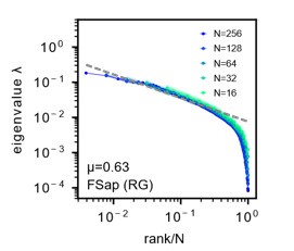
(2) The quantification of the degree of scale invariance is done using a ”collapse index” (CI), which could be better explained/motivated. The fact that the measure is computed only for the non-leading eigenvalues makes sense but it is not clear when originally introduced. How does this measure compare to other measures of the distance between distributions?
We thank you for raising this important point regarding the explanation and motivation for our Collapse Index (CI). We defined the Collapse Index (CI) instead of other measures of distance between distributions for two main reasons. First, the CI provides an intuitive quantification of the shift of the eigenspectrum motivated by our high-density theory for the ERM model (Eq. 3, Fig. 4A). This high-density theory is only valid for large eigenvalues excluding the leading ones, and hence we compute the CI measure with a similar restriction of the range of area integration. Second, when using distribution to assess the collapse (e.g., we can use kernel density method to estimate the distribution of eigenvalues and then calculate the KL divergence between the two distributions), it is necessary to first estimate the distributions. This estimation step introduces errors, such as inaccuracies in estimating the probability of large eigenvalues.
We agree that a clearer explanation would enhance the manuscript and thus have made modifications accordingly. The CI is now introduced more clearly in the Results section (lines 145-148) and further detailed in the Methods section (lines 630-636). We have also revised the CI diagram in Fig. 4A to better illustrate the shift concept using a more intuitive cartoon representation.
(3) The paper focuses on the case in which the dimensionality saturates to a finite value as the number of recorded neurons is increased. It would be useful to contrast with a case in which this does not occur. The paper would be strengthened by a comparison with Manley et al. 2024, which argued that, unlike this study, dimensionality of activity in spontaneously behaving head-fixed mice did not saturate.
Thank you for highlighting this comparison. We have included a discussion (lines 303-309) comparing our approach with Manley et al. (2024) [2]. While Manley et al. [2] primarily used shared variance component analysis (SVCA) to estimate neural dimensionality, they observed that using PCA led to dimensionality saturation (see Figure S4D, Manley et al. [2]), consistent with our findings (Fig. 2D). We acknowledge the value of SVCA as an alternative approach and agree that it is an interesting avenue for future research. In our study, we chose to use PCA for several reasons. PCA is a well-established and widely trusted method in the neuroscience community, with a proven track record of revealing meaningful patterns in neural data. Its mathematical properties are well understood, making it particularly suitable for our theoretical analysis. While we appreciate the insights that newer methods like SVCA can provide, we believe PCA remains the most appropriate tool for addressing our specific research questions.
(4) More importantly, we don’t understand why dimensionality saturates. For the rank plot given in Eq. 3,

where k is rank. Using this, one can estimate sums over eigenvalues by integrals. Focusing on the N-dependence, we have
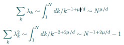
This gives
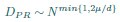
We don’t think you ever told us what mu/d was (see point 13 below), but in the discussion you implied that it was around 1/2 (line 249). In that case, D<sub>PR</sub> should be approximately linear in N. Could you explain why it isn’t?
Thank you for your careful derivation. Along this line of calculations you suggested, we have now added derivations on using the ERM spectrum to estimate the upper bound of the dimension in the Methods (section 4.14.4). To deduce D<sub>PR</sub> from the spectrum, we focus on the high-density region, where an analytical expression for large eigenvalues λ is given by:
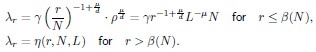
Here, d is dimension of functional space, L is the linear size of functional space, ρ is the neuron density and γ is the coefficient in Eq. (3), which only depends on d, µ and E(σ<sup>2</sup>). The primary difference between your derivation and ours is that the eigenvalue λ<sub>r</sub> decays rapidly after the threshold r \= β(N), which significantly affects the summations
 and
and  . Since we did not discuss the small eigenvalues in the article, we represent them here as an unknown function η(r,N,L).
The sum
is the trace of the covariance matrix C. As emphasized in the Methods section, without changing the properties the covariance spectrum, we always consider a normalized covariance matrix such that the mean neural activity variance E(σ<sup>2</sup>) = 1. Thus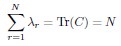
rather than
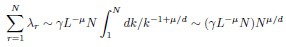
The issue stems from overlooking that Eq. (3) is valid only for large eigenvalues (λ > 1).
Using the Cauchy–Schwarz inequality, we have a upper bound of
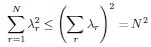
Conversely,
 provides a lower bound of :
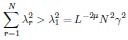
As a result, we must have
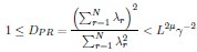
In random sampling (RSap), L is fixed. We thus must have a bounded dimensionality that is independent of N for our ERM model. In functional sampling (FSap), L varies while the neuronal density ρ is fixed, leading to a different scaling relationship of the upper bound, see Methods (section 4.14.4) for further discussion.
(5) The authors work directly with ROIs rather than attempting to separate the signals from each neuron in an ROI. It would be worth discussing whether this has a significant effect on the results.
We appreciate your thoughtful question on the potential impact of using ROIs. The use of ROIs likely does not impact our key findings since they are validated across multiple datasets with various recording techniques and animal models, from zebrafish calcium imaging to mouse brain multi-electrode recordings (see Figure S2, S24). The consistency of the scale-invariant covariance spectrum in diverse datasets suggests that ROIs in zebrafish data do not significantly alter the conclusions, and they together enhance the generalizability of our results. We highlight this in the Discussion section (lines 319-323).
(6) Does the Euclidean random matrix model allow the authors to infer the value of D or µ? Since the measured observables only depend on µ/D it seems that one cannot infer the latent dimension where distances between neurons are computed. Are there any experiments that one could, in principle, perform to measure D or mu? Currently the conclusion from the model and data is that D/µ is a large number so that the spectrum is independent of neuron density rho. What about the heterogeneity of the scales σ<sub>i</sub>, can this be constrained by data?
Measuring d and µ in the ERM Model
We agree with you that the individual values of d and µ cannot be determined separately from our analysis. In our analysis using the Euclidean Random Matrix (ERM) model, we fit the ratio µ/d, rather than the individual values of d (dimension of the functional space) or µ (exponent of the distance-dependent kernel function). This limitation is inherent because the model’s predictions for observable quantities, such as the distribution of pairwise correlation, are dependent solely on this ratio.
Currently there are no directly targeted experiments to measure d. The dimensions of the functional space is largely a theoretical construct: it could serve to represent latent variables encoding cognitive factors that are distributed throughout the brain or specific sensory or motor feature maps within a particular brain region. It may also be viewed as the embedding space to describe functional connectivity between neurons. Thus, a direct experimental measurement of the dimensions of the functional space could be challenging. Although there are variations in the biological interpretation of the functional space, the consistent scale invariance observed across various brain regions indicates that the neuronal relationships within the functional space can be described by a uniform slowly decaying kernel function.
Regarding the Heterogeneity of σ<sub>i</sub>
The heterogeneity of neuronal activity variances ( σ<sub>i</sub>) is a critical factor in our analysis. Our findings indicate that this heterogeneity:
(1) Enhances scale invariance: The covariance matrix spectrum, which incorporates the heterogeneity of
 , exhibits stronger scale invariance compared to the correlation matrix spectrum, which imposes
  for all neurons. This observation is supported by both experimental data and theoretical predictions from the ERM model, particularly in the intermediate density regime.
(2) Can be constrained by data: We fit a log-normal distribution to the experimentally observed σ<sup>2</sup> values to capture the heterogeneity in our model which leads to excellent agreement with data (section 4.8.1). Figure S10 provides evidence for this by directly comparing the eigenspectra obtained from experimental data (Fig S10A-F) with those generated by the fitted ERM model (Fig S10M-R). These results suggest that the data provides valuable information about the distribution of neuronal activity variances.
In conclusion, the ERM model and our analysis cannot separately determine d and µ. We also highlight that the neuronal activity variance heterogeneity, constrained by experimental data, plays a crucial role in improving the scale invariance.
(7) Does the fitting procedure for the positions x in the latent space recover a ground truth in your statistical regime (for the number of recorded neurons)? Suppose you sampled some neurons from a Euclidean random matrix theory. Does the MDS technique the authors use recover the correct distances?
While sampling neurons from a Euclidean random matrix model, we demonstrated numerically that the MDS technique can accurately recover the true distances, provided that the true parameter f(x) is known. To quantify the precision of recovery, we applied the CCA analysis (Section 4.9) and compared the true coordinates
 from the original Euclidean random matrix with the fitted coordinates
  obtained through our MDS procedure. The CCA correlation between the true and fitted coordinates in each spatial dimension is nearly 1 (the difference from 1 is less than 10<sup>−7</sup>). When fitting with experimental data, one source of error arises from parameter estimation. To evaluate this, we assess the estimation error of the fitted parameters. When we choose µ \= 0_.5 in our ERM model and then fit the distribution of the pairwise correlation (Eq. 21), the estimated parameter is
  = 0.503 ± 0._007 (standard deviation). Then, we use the MDS-recovered distances to fit the coordinates with the fitted kernel function
  , which is determined by the fitted parameter . The CCA correlation between the true and fitted coordinates in each direction remains nearly 1 (the difference from 1 is less than 10<sup>−5</sup>).
(8) l. 49: ”... both the dimensionality and covariance spectrum remain invariant ...”. Just to be clear, if the spectrum is invariant, then the dimensionality automatically is too. Correct?
Thanks for the question. In fact, there is no direct causal relationship between eigenvalue spectrum invariance and dimensionality invariance as we elaborate below and added discussions in lines 311-317. For eigenvalue spectrum invariance, we focus on the large eigenvalues, whereas dimensionality invariance considers the second order statistics of all eigenvalues. Consequently, the invariance results for these two concepts may differ. And dimensional and spectral invariance have different requirements:
(1) The condition for dimensional saturation is finite mean square covariance
The participation ratio D<sub>PR</sub> for random sampling (RSap) is given by Eq. 5:
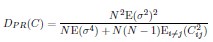
This expression becomes invariant as N → ∞ if the mean square covariance is finite. In contrast, neural dynamics models, such as the balanced excitatory-inhibitory (E-I) neural network [5], exhibit a different behavior, where
 , leading to unbounded dimensionality (see discussion lines 291-295, section 6.9 in SI).
(2) The requirements for spectral invariance involving the kernel function
In our Euclidean Random Matrix (ERM) model, the eigenvalue distribution follows:
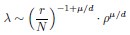
For spectral invariance to emerge: (1) The eigenvalue distribution must remain unchanged after sampling. (2) Since sampling reduces the neuronal density ρ. (3) The ratio µ/d must approach 0 to maintain invariance.
We can also demonstrate that D<sub>PR</sub> is independent of density ρ in the large N limit (see the answer of question 4).
In conclusion, there is no causal relationship between spectral invariance and dimensionality invariance. This is also the reason why we need to consider both properties separately in our analysis.
(9) In Eq. 1, the exact expression, which includes i=j, isn’t a lot harder than the one with i=j excluded. So why i≠j?
The choice is for illustration purposes. In Eq. 1, we wanted to demonstrate that the dimension saturates to a value independent of N. When dividing the numerator and denominator of this expression by N<sup>2</sup>, the term
 is independent of the neuron number N, but the term associated with the diagonal entries
  is of order O(1_/N_) and can be ignored for large N.
(10) Fig. 2D: Could you explain where the theory line comes from?
We first estimate
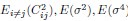 ] from all neurons, and then compute D<sub>PR</sub> for different neuron numbers N using Eq.5 (). This is further clarified in lines 511-512.
(11) l 94-5: ”It [scale invariance] is also absent when replacing the neural covariance matrix eigenvectors with random ones, keeping the eigenvalues identical (Fig. 2H).” If eigenvalues are identical, why does the spectrum change?
The eigenspectra of the covariance matrices in full size are the same by construction, but the eigenspectra of the sampled covariance matrices are different because the eigenvectors affect the sampling results. Please also refer to the construction process described in section 4.3 where this is also discussed: “The composite covariance matrix with substituted eigenvectors in (Fig. 2H) was created as described in the following steps. First, we generated a random orthogonal matrix U<sub>r<.sup> (based on the Haar measure) for the new eigenvectors. This was achieved by QR decomposition A=U<sub>r</sub>R of a random matrix A with i.i.d. entries A<sub>ij</sub> ∼ N(0_,1/N_). The composite covariance matrix C<sub>r</sub> was then defined as, where Λ is a diagonal matrix that contains the eigenvalues of C. Note that since all the eigenvalues are real and U<sub>r</sub> is orthogonal, the resulting C<sub>r</sub> is a real and symmetric matrix. By construction, C<sub>r</sub> and C have the same eigenvalues, but their sampled eigenspectra can differ.”
(12) Eq 3: There’s no dependence on the distribution of sigma. Is that correct?
Indeed, this is true in the high-density regime when the neuron density ρ is large. The p(λ) depends only on E(σ<sup>2</sup>) rather than the distribution of σ (see Eq. 8). However, in the intermediate density regime, p(λ) depends on the distribution of σ (see Eq.9 and Eq.10). In our analysis, we consider E(σ<sup>4</sup>) as a measure of heterogeneity.
(13) Please tell us the best fit values of µ/d.
This information now is added in the figure caption of Fig S10: µ/d \= [0_.456,0.258,0.205,0.262,0.302,0._308] in fish 1-6.
(14) l 133: ”The eigenspectrum is rho-independent whenever µ/d ≈ 0.”
It looks to me like rho sets the scale but not the shape. Correct? If so, why do we care about the overall scale – isn’t it the shape that’s important?
Yes, our study focuses on the overall scale not only the shape, because many models, such as the ERM with other kernel functions, random RNNs, Morrell’s latent model [4, 1], can exhibit a power-law spectrum. However, these models do not exhibit scale-invariance in terms of spectrum curve collapsing. Therefore, considering the overall scale reveal additional non-trivial phenomenon.
(15) Figs. 3 and 4: Are the grey dots the same as in previous figures? Either way, please specify what they are in the figure caption.
Yes, they are the same, and thank you for pointing it out. It has been specified in the figure caption now.
(16) Fig. 4B: Top is correlation matrix, bottom is covariance matrix, correct? If so, that should be explicit. If not, it should be clear what the plots are.
That is correct. Both matrices (correlation - top, covariance - bottom) are labeled in the figure caption and plot (text in the lower left corner).
(17) l 158: ”First, the shape of the kernel function f(x) over a small distance ...”. What does ”over a small distance” mean?
We thank you for seeking clarification on this point. We understand that the phrase ”over a small distance” could be made clearer. We made a revised explanation in lines 164-165 Here, “over a small distance” refers to modifications of the particular kernel function f(x) we use Eq. 11 near x \= 0 in the functional space, while preserving the overall power-law decay at larger distances. The t-distribution based f(x) (Eq. 11) has a natural parameter ϵ that describes the transition to near 0. So we modified f(x) in different ways, all within this interval of |x| ≤ ϵ, and considered different values of ϵ. Table S3 and Figure S7 provide a summary of these modifications. Figure S7 visually compares these modifications to the standard power-law kernel function, highlighting the differences in shape near x \= 0.
Our findings indicate that these alterations to the kernel function at small distances do not significantly affect the distribution of large eigenvalues in the covariance spectrum. This supports our conclusion that the large eigenvalues are primarily determined by the slow decay of the kernel function at larger distances in the functional space, as this characteristic governs the overall correlations in neural activity.
(18) l390
 . This x<sub>i</sub> is, we believe, different from the x<sub>i</sub> which is position in feature space. Given the difficulty of this paper, it doesn’t help to use the same symbol to mean two different things. But maybe we’re wrong?
Thank you for your careful reading and suggestion. Indeed here x<sub>i</sub> was representing activity rather than feature space position. We have thus revised the notation (Line 390 has been updated to line 439 as well.):
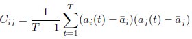
In this revised notation: a<sub>i</sub>(t) represents the neural activity of neuron i at time t (typically the firing rate we infer from calcium imaging).
 is simply the mean activity of neuron i across time. Meanwhile, we’ll keep x<sub>i</sub> exclusively for denoting positions in the functional space.
This change should make it much easier to distinguish between neural activity measurements and spatial coordinates in the functional space.
(19) Eq. 19: is it correct that g(u) is not normalized to 1? If so, does that matter?
It is correct that the approximation of g(u) is not normalized to 1, as Eq. 19 provides an approximation suitable only for small pairwise distances (i.e., large correlation). Therefore, we believe this does not pose an issue. We have newly added this note in lines 691-693.
(20) I get a different answer in Eq. 20:
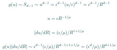
Whereas in Eq. 20,
 µ
µWhich is correct?
Thank you for your careful derivation. We believe the difference arises in the calculation of g(u).In our calculations:
 ,
,(Your first equation seems to missed an 1_/µ_ in R’s exponent.)
 ,
,That is, Eq. 20 is correct. From these, we obtain
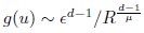
rather than
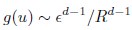
We hope this clarifies the question.
(21) I’m not sure we fully understand the CCA analysis. First, our guess as to what you did: After sampling (either Asap or Fsap), you used ERM to embed the neurons in a 2-D space, and then applied canonical correlation analysis (CCA). Is that correct? If so, it would be nice if that were more clear.
We first used ERM to embed all the neurons in a 2-D functional space, before any sampling. Once we have the embedding, we can quantify how similar the functional coordinates are with the anatomical coordinates using R<sub>CCA</sub> (section 2.4). We can then use the anatomical and functional coordinates to perform ASap and FSap, respectively. Our theory in section 2.4 predicts the effect on dimension under these samplings given the value of R<sub>CCA</sub> estimated earlier (Fig. 5D). The detailed description of the CCA analysis is in section 4.9, where we explain how CCA is used to find the axes in both anatomical and functional spaces that maximize the correlation between projections of neuron coordinates.
As to how you sampled under Fsap, I could not figure that out – even after reading supplementary information. A clearer explanation would be very helpful.
Thank you for your feedback. Functional sampling (FSap) entails the expansion of regions of interest (ROIs) within the functional space, as illustrated in Figure 5A, concurrently with the calculation of the covariance matrix for all neurons contained within the ROI. Technically, we implemented the sampling using the RG approach [6], which is further elaborated in Section 4.12 (lines 852-899), quoted below.
Stage (i): Iterative Clustering We begin with N</sub>0</sub> neurons, where N</sub>0</sub> is assumed to be a power of 2. In the first iteration, we compute Pearson’s correlation coefficients for all neuron pairs. We then search greedily for the most correlated pairs and group the half pairs with the highest correlation into the first cluster; the remaining neurons form the second cluster. For each pair (a,b), we define a coarse-grained variable according to:
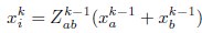 ,
,Where
 normalizes the average to ensure unit nonzero activity. This process reduces the number of neurons to N<sub>1</sub> = N<sub>0</sub>/2. In subsequent iterations, we continue grouping the most correlated pairs of the coarse-grained neurons, iteratively reducing the number of neurons by half at each step. This process continues until the desired level of coarse-graining is achieved.
When applying the RG approach to ERM, instead of combining neural activity, we merge correlation matrices to traverse different scales. During the _k_th iteration, we compute the coarse-grained covariance as:
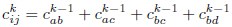
and the variance as:
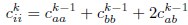
Following these calculations, we normalize the coarse-grained covariance matrix to ensure that all variances are equal to one. Note that these coarse-grained covariances are only used in stage (i) and not used to calculate the spectrum.
Stage (ii): Eigenspectrum Calculation The calculation of eigenspectra at different scales proceeds through three sequential steps. First, for each cluster identified in Stage (i), we compute the covariance matrix using the original firing rates of neurons within that cluster (not the coarse-grained activities). Second, we calculate the eigenspectrum for each cluster. Finally, we average these eigenspectra across all clusters at a given iteration level to obtain the representative eigenspectrum for that scale.
In stage (ii), we calculate the eigenspectra of the sub-covariance matrices across different cluster sizes as described in [6]. Let N<sub>0</sub> = 2<sup>n</sub> be the original number of neurons. To reduce it to size N \= N<sub>0</sub>/2<sup>k</sup> = 2<sup>n-k</sup>, where k is the kth reduction step, consider the coarse-grained neurons in step n − k in stage (i). Each coarse-grained neuron is a cluster of 2<sup>n-k</sup> neurons. We then calculate spectrum of the block of the original covariance matrix corresponding to neurons of each cluster (there are 2<sup>k</sup> such blocks). Lastly, an average of these 2<sup>k</sup> spectra is computed.
For example, when reducing from N<sub>0</sub> = 2<sup>3</sup> = 8 to N \= 2<sup>3−1</sup> = 4 neurons (k \= 1), we would have two clusters of 4 neurons each. We calculate the eigenspectrum for each 4x4 block of the original covariance matrix, then average these two spectra together. To better understand this process through a concrete example, consider a hypothetical scenario where a set of eight neurons, labeled 1,2,3,...,7,8, are subjected to a two-step clustering procedure. In the first step, neurons are grouped based on their maximum correlation pairs, for example, resulting in the formation of four pairs: {1,2},{3,4},{5,6}, and {7,8} (see Fig. S22). Subsequently, the neurons are further grouped into two clusters based on the results of the RG step mentioned above. Specifically, if the correlation between the coarse-grained variables of the pair {1,2} and the pair {3,4} is found to be the largest among all other pairs of coarse-grained variables, the first group consists of neurons {1,2,3,4}, while the second group contains neurons {5,6,7,8}. Next, take the size of the cluster N = 4 for example. The eigenspectra of the covariance matrices of the four neurons within each cluster are computed. This results in two eigenspectra, one for each cluster. The correlation matrices used to compute the eigenspectra of different sizes do not involve coarse-grained neurons. It is the real neurons 1,2,3,...,7,8, but with expanding cluster sizes. Finally, the average of the eigenspectra of the two clusters is calculated.
(22) Line 37: ”even if two cell assemblies have the same D<sub>PR</sub>, they can have different shapes.” What is meant by shape here isn’t clear.
Thank you for pointing out this potential ambiguity. The “shape” here refers to the geometric configuration of the neural activity space characterized as a highdimensional ellipsoid by the covariance. Specifically, if we denote the eigenvalues of the covariance matrix as λ<sub>1</sub>,λ<sub>2</sub>,...,λ<sub>N</sub>, then
 corresponds to the length of the i-th semi-axis of this ellipsoid (Figure 1B). As shown in Figure 1C, two neural populations with the same dimensionality (D<sub>PR</sub> = 25/11 ≈ 2.27) exhibit different eigenvalue spectra, leading to differently shaped ellipsoids. This clarification is now included in lines 39-40.
(23) Please discuss if any information about the latent dimension or kernel function can be inferred from the measurements.
Same as comment(6): we would like to clarify that in our analysis using the Euclidean Random Matrix (ERM) model, we fit the ratio µ/d, rather than the individual values of d (dimension of the functional space) or µ (exponent of the distancedependent kernel function). This limitation is inherent because the model’s predictions for observable quantities, such as the eigenvalue spectrum of the covariance matrix, are dependent solely on this ratio.
For the kernel function, once the d is chosen, we can infer the general shape of the kernel function from data (Figs S12 and S13), up to a certain extent (see also lines 164-166). In particular, we can compare the eigenspectrum of the simulation results for different kernel functions with the eigenspectrum of our data. This allows us to qualitatively exclude certain kernel functions, such as the exponential and Gaussian kernels (Fig. S4), which show clear differences from our data.
References
(1) M. C. Morrell, I. Nemenman, A. Sederberg, Neural criticality from effective latent variables. eLife 12, RP89337 (2024).
(2) J. Manley, S. Lu, K. Barber, J. Demas, H. Kim, D. Meyer, F. M. Traub, A. Vaziri, Simultaneous, cortex-wide dynamics of up to 1 million neurons reveal unbounded scaling of dimensionality with neuron number. Neuron (2024).
(3) S. A. Moosavi, S. S. R. Hindupur, H. Shimazaki, Population coding under the scale-invariance of high-dimensional noise (2024).
(4) M. C. Morrell, A. J. Sederberg, I. Nemenman, Latent dynamical variables produce signatures of spatiotemporal criticality in large biological systems. Physical Review Letters 126, 118302 (2021).
(5) A. Renart, J. De La Rocha, P. Bartho, L. Hollender, N. Parga, A. Reyes, K. D. Harris, The asynchronous state in cortical circuits. science 327, 587–590 (2010).
(6) L. Meshulam, J. L. Gauthier, C. D. Brody, D. W. Tank, W. Bialek, Coarse graining, fixed points, and scaling in a large population of neurons. Physical Review Letters 123, 178103 (2019).
-
-
www.biorxiv.org www.biorxiv.org
-
Author response:
The following is the authors’ response to the original reviews.
Response to Reviewer #1:
Thank you for the careful reading and the positive evaluation of our manuscript. As you mentioned, the present study tried to address the question of how the lost genomic functions could be compensated by evolutionary adaptation, indicating the potential mechanism of "constructive" rather than "destructive" evolution. Thank you for the instructive comments that helped us to improve the manuscript. We sincerely hope the revised manuscript and the following point-to-point response meet your concerns.
- Line 80 "Growth Fitness" is this growth rate?
Yes. The sentence was revised as follows.
(L87-88) “The results demonstrated that most evolved populations (Evos) showed improved growth rates, in which eight out of nine Evos were highly significant (Fig. 1B, upper).”
-
Line 94 a more nuanced understanding of r/K selection theory, allows for trade-ups between R and K, as well as trade-offs. This may explain why you did not see a trade-off between growth and carrying capacity in this study. See this paper https://doi.org/10.1038/s41396-023-01543-5. Overall, your evos lineages evolved higher growth rates and lower carrying capacity (Figures 1B, C, E). If selection was driving the evolution of higher growth rates, it may have been that there was no selective pressure to maintain high carrying capacity. This means that the evolutionary change you observed in carrying capacity may have been neutral "drift" of the carrying capacity trait, during selection for growth rate, not because of a trade-off between R and K. This is especially likely since carrying capacity declined during evolution. Unless the authors have convincing evidence for a tradeoff, I suggest they remove this claim.
-
Line 96 the authors introduce a previous result where they use colony size to measure growth rate, this finding needs to be properly introduced and explained so that we can understand the context of the conclusion.
-
Line 97 This sentence "the collapse of the trade-off law likely resulted from genome reduction." I am not sure how the authors can draw this conclusion, what is the evidence supporting that the genome size reduction causes the breakdown of the tradeoff between R and K (if there was a tradeoff)?
Thank you for the reference information and the thoughtful comments. The recommended paper was newly cited, and the description of the trade-off collapse was deleted. Accordingly, the corresponding paragraph was rewritten as follows.
(L100-115) “Intriguingly, a positive correlation was observed between the growth fitness and the carrying capacity of the Evos (Fig. 1D). It was somehow consistent with the positive correlations between the colony growth rate and the colony size of a genome-reduced strain 11 and between the growth rates and the saturated population size of an assortment of genome reduced strains 13. Nevertheless, the negative correlation between growth rate and carrying capacity, known as the r/K selection30,31 was often observed as the trade-off relationship between r and K in the evolution and ecology studies 32 33,34. As the r/K trade-off was proposed to balance the cellular metabolism that resulted from the cost of enzymes involved 34, the deleted genes might play a role in maintaining the metabolism balance for the r/K correlation. On the other hand, the experimental evolution (i.e., serial transfer) was strictly performed within the exponential growth phase; thus, the evolutionary selection was supposed to be driven by the growth rate without selective pressure to maintain the carrying capacity. The declined carrying capacity might have been its neutral "drift" but not a trade-off to the growth rate. Independent and parallel experimental evolution of the reduced genomes selecting either r or K is required to clarify the actual mechanisms.”
- Line 103 Genome mutations. The authors claim that there are no mutations in parallel but I see that there is a 1199 base pair deletion in eight of the nine evo strains (Table S3). I would like the author to mention this and I'm actually curious about why the authors don't consider this parallel evolution.
Thank you for your careful reading. According to your comment, we added a brief description of the 1199-bp deletion detected in the Evos as follows.
(L119-122) “The number of mutations largely varied among the nine Evos, from two to 13, and no common mutation was detected in all nine Evos (Table S3). A 1,199-bp deletion of insH was frequently found in the Evos (Table S3, highlighted), which well agreed with its function as a transposable sequence.”
- Line 297 Please describe the media in full here - this is an important detail for the evolution experiment. Very frustrating to go to reference 13 and find another reference, but no details of the method. Looked online for the M63 growth media and the carbon source is not specified. This is critical for working out what selection pressures might have driven the genetic and transcriptional changes that you have measured. For example, the parallel genetic change in 8/9 populations is a deletion of insH and tdcD (according to Table S3). This is acetate kinase, essential for the final step in the overflow metabolism of glucose into acetate. If you have a very low glucose concentration, then it could be that there was selection to avoid fermentation and devote all the pyruvate that results from glycolysis into the TCA cycle (which is more efficient than fermentation in terms of ATP produced per pyruvate).
Sorry for the missing information on the medium composition, which was additionally described in the Materials and Methods. The glucose concentration in M63 was 22 mM, which was supposed to be enough for bacterial growth. Thank you for your intriguing thinking about linking the medium component to the genome mutation-mediated metabolic changes. As there was no experimental result regarding the biological function of gene mutation in the present study, please allow us to address this issue in our future work.
(L334-337) “In brief, the medium contains 62 mM dipotassium hydrogen phosphate, 39 mM potassium dihydrogen phosphate, 15 mM ammonium sulfate, 15 μM thiamine hydrochloride, 1.8 μM Iron (II) sulfate, 0.2 mM magnesium sulfate, and 22 mM glucose.”
-
Line 115. I do not understand this argument "They seemed highly related to essentiality, as 11 out of 49 mutated genes were essential (Table S3)." Is this a significant enrichment compared to the expectation, i.e. the number of essential genes in the genome? This enrichment needs to be tested with a Hypergeometric test or something similar.
-
Also, "As the essential genes were known to be more conserved than nonessential ones, the high frequency of the mutations fixed in the essential genes suggested the mutation in essentiality for fitness increase was the evolutionary strategy for reduced genome." I do not think that there is enough evidence to support this claim, and it should be removed.
Sorry for the unclear description. Yes, the mutations were significantly enriched in the essential genes (11 out of 45 genes) compared to the essential genes in the whole genome (286 out of 3290 genes). The improper description linking the mutation in essential genes to the fitness increase was removed, and an additional explanation on the ratio of essential genes was newly supplied as follows.
(L139-143) “The ratio of essential genes in the mutated genes was significantly higher than in the total genes (286 out of 3290 genes, Chi-square test p=0.008). As the essential genes were determined according to the growth35 and were known to be more conserved than nonessential ones 36,37, the high frequency of the mutations fixed in the essential genes was highly intriguing and reasonable.”
- Line 124 Regarding the mutation simulations, I do not understand how the observed data were compared to the simulated data, and how conclusions were drawn. Can the authors please explain the motivation for carrying out this analysis, and clearly explain the conclusions?
Random simulation was additionally explained in the Materials and Methods and the conclusion of the random simulation was revised in the Results, as follows.
(L392-401) “The mutation simulation was performed with Python in the following steps. A total of 65 mutations were randomly generated on the reduced genome, and the distances from the mutated genomic locations to the nearest genomic scars caused by genome reduction were calculated. Subsequently, Welch's t-test was performed to evaluate whether the distances calculated from the random mutations were significantly longer or shorter than those calculated from the mutations that occurred in Evos. The random simulation, distance calculation, and statistic test were performed 1,000 times, which resulted in 1,000 p values. Finally, the mean of p values (μp) was calculated, and a 95% reliable region was applied. It was used to evaluate whether the 65 mutations in the Evos were significantly close to the genomic scars, i.e., the locational bias.”
(L148-157) “Random simulation was performed to verify whether there was any bias or hotspot in the genomic location for mutation accumulation due to the genome reduction. A total of 65 mutations were randomly generated on the reduced genome (Fig. 2B), and the genomic distances from the mutations to the nearest genome reduction-mediated scars were calculated. Welch's t-test was performed to evaluate whether the genomic distances calculated from random mutations significantly differed from those from the mutations accumulated in the Evos. As the mean of p values (1,000 times of random simulations) was insignificant (Fig. 2C, μp > 0.05), the mutations fixed on the reduced genome were either closer or farther to the genomic scars, indicating there was no locational bias for mutation accumulation caused by genome reduction.”
-
Line 140 The authors should give some background here - explain the idea underlying chromosomal periodicity of the transcriptome, to help the reader understand this analysis.
-
Line 142 Here and elsewhere, when referring to a method, do not just give the citation, but also refer to the methods section or relevant supplementary material.
The analytical process (references and methods) was described in the Materials and Methods, and the reason we performed the chromosomal periodicity was added in the Results as follows.
(L165-172) “As the E. coli chromosome was structured, whether the genome reduction caused the changes in its architecture, which led to the differentiated transcriptome reorganization in the Evos, was investigated. The chromosomal periodicity of gene expression was analyzed to determine the structural feature of genome-wide pattern, as previously described 28,38. The analytical results showed that the transcriptomes of all Evos presented a common six-period with statistical significance, equivalent to those of the wild-type and ancestral reduced genomes (Fig. 3A, Table S4).”
- Line 151 "The expression levels of the mutated genes were higher than those of the remaining genes (Figure 3B)"- did this depend on the type of mutation? There were quite a few early stops in genes, were these also more likely to be expressed? And how about the transcriptional regulators, can you see evidence of their downstream impact?
Sorry, we didn't investigate the detailed regulatory mechanisms of 49 mutated genes, which was supposed to be out of the scope of the present study. Fig. 3B was the statistical comparison between 3225 and 49 genes. It didn't mean that all mutated genes expressed higher than the others. The following sentences were added to address your concern.
(L181-185) “As the regulatory mechanisms or the gene functions were supposed to be disturbed by the mutations, the expression levels of individual genes might have been either up- or down-regulated. Nevertheless, the overall expression levels of all mutated genes tended to be increased. One of the reasons was assumed to be the mutation essentiality, which remained to be experimentally verified.”
- Line 199 onward. The authors used WGCNA to analyze the gene expression data of evolved organisms. They identified distinct gene modules in the reduced genome, and through further analysis, they found that specific modules were strongly associated with key biological traits like growth fitness, gene expression changes, and mutation rates. Did the authors expect that there was variation in mutation rate across their populations? Is variation from 3-16 mutations that they observed beyond the expectation for the wt mutation rate? The genetic causes of mutation rate variation are well understood, but I could not see any dinB, mutT,Y, rad, or pol genes among the discovered mutations. I would like the authors to justify the claim that there was mutation rate variation in the evolved populations.
Thank you for the intriguing thinking. We don't think the mutation rates were significantly varied across the nine populations, as no mutation occurred in the MMR genes, as you noticed. Our previous study showed that the spontaneous mutation rate of the reduced genome was higher than that of the wild-type genome (Nishimura et al., 2017, mBio). As nonsynonymous mutations were not detected in all nine Evos, the spontaneous mutation rate couldn't be calculated (because it should be evaluated according to the ratio of nonsynonymous and synonymous single-nucleotide substitutions in molecular evolution). Therefore, discussing the mutation rate in the present study was unavailable. The following sentence was added for a better understanding of the gene modules.
(L242-245) “These modules M2, M10 and M16 might be considered as the hotspots for the genes responsible for growth fitness, transcriptional reorganization, and mutation accumulation of the reduced genome in evolution, respectively.”
- Line 254 I get the idea of all roads leading to Rome, which is very fitting. However, describing the various evolutionary strategies and homeostatic and variable consequence does not sound correct - although I am not sure exactly what is meant here. Looking at Figure 7, I will call strategy I "parallel evolution", that is following the same or similar genetic pathways to adaptation and strategy ii I would call divergent evolution. I am not sure what strategy iii is. I don't want the authors to use the terms parallel and divergent if that's not what they mean. My request here would be that the authors clearly describe these strategies, but then show how their results fit in with the results, and if possible, fit with the naming conventions, of evolutionary biology.
Thank you for your kind consideration and excellent suggestion. It's our pleasure to adopt your idea in tour study. The evolutionary strategies were renamed according to your recommendation. Both the main text and Fig. 7 were revised as follows.
(L285-293) “Common mutations22,44 or identical genetic functions45 were reported in the experimental evolution with different reduced genomes, commonly known as parallel evolution (Fig. 7, i). In addition, as not all mutations contribute to the evolved fitness 22,45, another strategy for varied phenotypes was known as divergent evolution (Fig. 7, ii). The present study accentuated the variety of mutations fixed during evolution. Considering the high essentiality of the mutated genes (Table S3), most or all mutations were assumed to benefit the fitness increase, partially demonstrated previously 20. Nevertheless, the evolved transcriptomes presented a homeostatic architecture, revealing the divergent to convergent evolutionary strategy (Fig. 7, iii).”
Author response image 1.
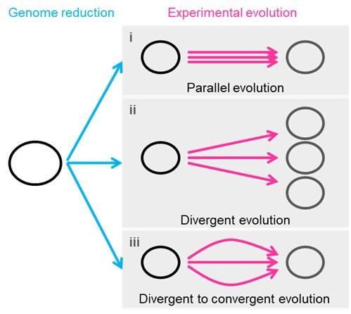
- Line 327 Growth rates/fitness. I don't think this should be called growth fitness- a rate is being calculated. I would like the authors to explain how the times were chosen - do the three points have to be during the log phase? Can you also explain what you mean by choosing three ri that have the largest mean and minor variance?
Sorry for the confusing term usage. The fitness assay was changed to the growth assay. Choosing three ri that have the largest mean and minor variance was to avoid the occasional large values (blue circle), as shown in the following figure. In addition, the details of the growth analysis can be found at https://doi.org/10.3791/56197 (ref. 59), where the video of experimental manipulation, protocol, and data analysis is deposited. The following sentence was added in accordance.
Author response image 2.
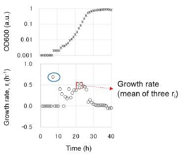
(L369-371) “The growth rate was determined as the average of three consecutive ri, showing the largest mean and minor variance to avoid the unreliable calculation caused by the occasionally occurring values. The details of the experimental and analytical processes can be found at https://doi.org/10.3791/56197.”
- Line 403 Chromosomal periodicity analysis. The windows chosen for smoothing (100kb) seem big. Large windows make sense for some things - for example looking at how transcription relates to DNA replication timing, which is a whole-genome scale trend. However, here the authors are looking for the differences after evolution, which will be local trends dependent on specific genes and transcription factors. 100kb of the genome would carry on the order of one hundred genes and might be too coarse-grained to see differences between evos lineages.
Thank you for the advice. We agree that the present analysis focused on the global trend of gene expression. Varying the sizes may lead to different patterns. Additional analysis was performed according to your comment. The results showed that changes in window size (1, 10, 50, 100, and 200 kb) didn't alter the periodicity of the reduced genome, which agreed with the previous study on a different reduced genome MDS42 of a conserved periodicity (Ying et al., 2013, BMC Genomics). The following sentence was added in the Materials and Methods.
(L460-461) “Note that altering the moving average did not change the max peak.”
- Figures - the figures look great. Figure 7 needs a legend.
Thank you. The following legend was added.
(L774-777) “Three evolutionary strategies are proposed. Pink and blue arrowed lines indicate experimental evolution and genome reduction, respectively. The size of the open cycles represents the genome size. Black and grey indicate the ancestor and evolved genomes, respectively.”
Response to Reviewer #2:
Thank you for reviewing our manuscript and for your fruitful comments. We agree that our study leaned towards elaborating observed findings rather than explaining the detailed biological mechanisms. We focused on the genome-wide biological features rather than the specific biological functions. The underlying mechanisms indeed remained unknown, leaving the questions as you commented. We didn't perform the fitness assay on reconstituted (single and combinatorial) mutants because the research purpose was not to clarify the regulatory or metabolic mechanisms. It's why the RNA-Seq analysis provided the findings on genome-wide patterns and chromosomal view, which were supposed to be biologically valuable. We did understand your comments and complaints that the conclusions were biologically meaningless, as ALE studies that found the specific gene regulation or improved pathway was the preferred story in common, which was not the flow of the present study.
For this reason, our revision may not address all these concerns. Considering your comments, we tried our best to revise the manuscript. The changes made were highlighted. We sincerely hope the revision and the following point-to-point response are acceptable.
Major remarks:
(1) The authors outlined the significance of ALE in genome-reduced organisms and important findings from published literature throughout the Introduction section. The description in L65-69, which I believe pertains to the motivation of this study, seems vague and insufficient to convey the novelty or necessity of this study i.e. it is difficult to grasp what aspects of genome-reduced biology that this manuscript intends to focus/find/address.
Sorry for the unclear writing. The sentences were rewritten for clarity as follows.
(L64-70) “Although the reduced growth rate caused by genome reduction could be recovered by experimental evolution, it remains unclear whether such an evolutionary improvement in growth fitness was a general feature of the reduced genome and how the genome-wide changes occurred to match the growth fitness increase. In the present study, we performed the experimental evolution with a reduced genome in multiple lineages and analyzed the evolutionary changes of the genome and transcriptome.”
(2) What is the rationale behind the lineage selection described in Figure S1 legend "Only one of the four overnight cultures in the exponential growth phase (OD600 = 0.01~0.1) was chosen for the following serial transfer, highlighted in red."?
The four wells (cultures of different initial cell concentrations) were measured every day, and only the well that showed OD600=0.01~0.1 (red) was transferred with four different dilution rates (e.g., 10, 100, 1000, and 10000 dilution rates). It resulted in four wells of different initial cell concentrations. Multiple dilutions promised that at least one of the wells would show the OD600 within the range of 0.01 to 0.1 after the overnight culture. They were then used for the next serial transfer. Fig. S1 provides the details of the experimental records. The experimental evolution was strictly controlled within the exponential phase, quite different from the commonly conducted ALE that transferred a single culture in a fixed dilution rate. Serial transfer with multiple dilution rates was previously applied in our evolution experiments and well described in Nishimura et al., 2017, mBio; Lu et al., 2022, Comm Biol; Kurokawa et al., 2022, Front Microbiol, etc. The following sentence was added in the Materials and Methods.
(L344-345) “Multiple dilutions changing in order promised at least one of the wells within the exponential growth phase after the overnight culture.”
(3) The measured growth rate of the end-point 'F2 lineage' shown in Figure S2 seemed comparable to the rest of the lineages (A1 to H2), but the growth rate of 'F2' illustrated in Figure 1B indicates otherwise (L83-84). What is the reason for the incongruence between the two datasets?
Sorry for the unclear description. The growth rates shown in Fig. S2 were obtained during the evolution experiment using the daily transfer's initial and final OD600 values. The growth rates shown in Fig. 1B were obtained from the final population (Evos) growth assay and calculated from the growth curves (biological replication, N=4). Fig. 1B shows the precisely evaluated growth rates, and Fig. S2 shows the evolutionary changes in growth rates. Accordingly, the following sentence was added to the Results.
(L84-87) “As the growth increases were calculated according to the initial and final records, the exponential growth rates of the ancestor and evolved populations were obtained according to the growth curves for a precise evaluation of the evolutionary changes in growth.”
(4) Are the differences in growth rate statistically significant in Figure 1B?
Eight out of nine Evos were significant, except F2. The sentences were rewritten and associated with the revised Fig. 1B, indicating significance.
(L87-90) “The results demonstrated that most evolved populations (Evos) showed improved growth rates, in which eight out of nine Evos were highly significant (Fig. 1B, upper). However, the magnitudes of growth improvement were considerably varied, and the evolutionary dynamics of the nine lineages were somehow divergent (Fig. S2).”
(5) The evolved lineages showed a decrease in their maximal optical densities (OD600) compared to the ancestral strain (L85-86). ALE could accompany changes in cell size and morphologies, (doi: 10.1038/s41586-023-06288-x; 10.1128/AEM.01120-17), which may render OD600 relatively inaccurate for cell density comparison. I suggest using CFU/mL metrics for the sake of a fair comparison between Anc and Evo.
The methods evaluating the carrying capacity (i.e., cell density, population size, etc.) do not change the results. Even using CFU is unfair for the living cells that can not form colonies and unfair if the cell size changes. Optical density (OD600) provides us with the temporal changes of cell growth in a 15-minute interval, which results in an exact evaluation of the growth rate in the exponential phase. CFU is poor at recording the temporal changes of population changes, which tend to result in an inappropriate growth rate. Taken together, we believe that our method was reasonable and reliable. We hope you can accept the different way of study.
(6) Please provide evidence in support of the statement in L115-119. i.e. statistical analysis supporting that the observed ratio of essential genes in the mutant pool is not random.
The statistic test was performed, and the following sentence was added.
(L139-141) “The ratio of essential genes in the mutated genes was significantly higher than in the total genes (286 out of 3290 genes, Chi-square test p=0.008).”
(7) The assumption that "mutation abundance would correlate to fitness improvement" described in L120-122: "The large variety in genome mutations and no correlation of mutation abundance to fitness improvement strongly suggested that no mutations were specifically responsible or crucially essential for recovering the growth rate of the reduced genome" is not easy to digest, in the sense that (i) the effect of multiple beneficial mutations are not necessarily summative, but are riddled with various epistatic interactions (doi: 10.1016/j.mec.2023.e00227); (ii) neutral hitchhikers are of common presence (you could easily find reference on this one); (iii) hypermutators that accumulate greater number of mutations in a given time are not always the eventual winners in competition games (doi: 10.1126/science.1056421). In this sense, the notion that "mutation abundance correlates to fitness improvement" in L120-122 seems flawed (for your perusal, doi: 10.1186/gb-2009-10-10-r118).
Sorry for the improper description and confusing writing, and thank you for the fruitful knowledge on molecular evolution. The sentence was deleted, and the following one was added.
(L145-146) “Nevertheless, it was unclear whether and how these mutations were explicitly responsible for recovering the growth rate of the reduced genome.”
(8) Could it be possible that the large variation in genome mutations in independent lineages results from a highly rugged fitness landscape characterized by multiple fitness optima (doi: 10.1073/pnas.1507916112)? If this is the case, I disagree with the notion in L121-122 "that no mutations were specifically responsible or crucially essential" It does seem to me that, for example, the mutations in evo A2 are specifically responsible and essential for the fitness improvement of evo A2 in the evolutionary condition (M63 medium). Fitness assessment of individual (or combinatorial) mutants reconstituted in the Ancestral background would be a bonus.
Thank you for the intriguing thinking. The sentence was deleted. Please allow us to adapt your comment to the manuscript as follows.
(L143-145) “The large variety of genome mutations fixed in the independent lineages might result from a highly rugged fitness landscape 38.”
(9) L121-122: "...no mutations were specifically responsible or crucially essential for recovering the growth rate of the reduced genome". Strictly speaking, the authors should provide a reference case of wild-type E. coli ALE in order to reach definitive conclusions that the observed mutation events are exclusive to the genome-reduced strain. It is strongly recommended that the authors perform comparative analysis with an ALEed non-genome-reduced control for a more definitive characterization of the evolutionary biology in a genome-reduced organism, as it was done for "JCVI-syn3.0B vs non-minimal M. mycoides" (doi: 10.1038/s41586-023-06288-x) and "E. coli eMS57 vs MG1655" (doi: 10.1038/s41467-019-08888-6).
The improper description was deleted in response to comments 7 and 8. The mentioned references were cited in the manuscript (refs 21 and 23). Thank you for the experimental advice. We are sorry that the comparison of wild-type and reduced genomes was not in the scope of the present study and will probably be reported soon in our future work.
(10) L146-148: "The homeostatic periodicity was consistent with our previous findings that the chromosomal periodicity of the transcriptome was independent of genomic or environmental variation" A Previous study also suggested that the amplitudes of the periodic transcriptomes were significantly correlated with the growth rates (doi: 10.1093/dnares/dsaa018). Growth rates of 8/9 Evos were higher compared to Anc, while that of Evo F2 remained similar. Please comment on the changes in amplitudes of the periodic transcriptomes between Anc and each Evo.
Thank you for the suggestion. The correlation between the growth rates and the amplitudes of chromosomal periodicity was statistically insignificant (p>0.05). It might be a result of the limited data points. Compared with the only nine data points in the present study, the previous study analyzed hundreds of transcriptomes associated with the corresponding growth rates, which are suitable for statistical evaluation. In addition, the changes in growth rates were more significant in the previous study than in the present study, which might influence the significance. It's why we did not discuss the periodic amplitude.
(11) Please elaborate on L159-161: "It strongly suggested the essentiality mutation for homeostatic transcriptome architecture happened in the reduced genome.".
Sorry for the improper description. The sentence was rewritten as follows.
(L191-193) “The essentiality of the mutations might have participated in maintaining the homeostatic transcriptome architecture of the reduced genome.”
(12) Is FPKM a valid metric for between-sample comparison? The growing consensus in the community adopts Transcripts Per Kilobase Million (TPM) for comparing gene expression levels between different samples (Figure 3B; L372-379).
Sorry for the unclear description. The FPKM indicated here was globally normalized, statistically equivalent to TPM. The following sentence was added to the Materials and Methods.
(L421-422) “The resulting normalized FPKM values were statistically equivalent to TPM.”
(13) Please provide % mapped frequency of mutations in Table S3.
They were all 100%. The partially fixed mutations were excluded in the present study. The following sentence was added to the caption of Table S3.
(Supplementary file, p 9) “Note that the entire population held the mutations, i.e., 100% frequency in DNA sequencing.”
(14) To my knowledge, M63 medium contains glucose and glycerol as carbon sources. The manuscript would benefit from discussing the elements that impose selection pressure in the M63 culture condition.
Sorry for the missing information on M63, which contains 22 mM glucose as the only carbon source. The medium composition was added in the Materials and Methods, as follows.
(L334-337) “In brief, the medium contains 62 mM dipotassium hydrogen phosphate, 39 mM potassium dihydrogen phosphate, 15 mM ammonium sulfate, 15 μM thiamine hydrochloride, 1.8 μM Iron (II) sulfate, 0.2 mM magnesium sulfate, and 22 mM glucose.”
(15) The RNA-Seq datasets for Evo strains seemed equally heterogenous, just as their mutation profiles. However, the missing element in their analysis is the directionality of gene expression changes. I wonder what sort of biological significance can be derived from grouping expression changes based solely on DEGs, without considering the magnitude and the direction (up- and down-regulation) of changes? RNA-seq analysis in its current form seems superficial to derive biologically meaningful interpretations.
We agree that most studies often discuss the direction of transcriptional changes. The present study aimed to capture a global view of the magnitude of transcriptome reorganization. Thus, the analyses focused on the overall features, such as the abundance of DEGs, instead of the details of the changes, e.g., the up- and down-regulation of DEGs. The biological meaning of the DEGs' overview was how significantly the genome-wide gene expression fluctuated, which might be short of an in-depth view of individual gene expression. The following sentence was added to indicate the limitation of the present analysis.
(L199-202) “Instead of an in-depth survey on the directional changes of the DEGs, the abundance and functional enrichment of DEGs were investigated to achieve an overview of how significant the genome-wide fluctuation in gene expression, which ignored the details of individual genes.”
Minor remarks
(1) L41: brackets italicized "(E. coli)".
It was fixed as follows.
(L40) “… Escherichia coli (E. coli) cells …”
(2) Figure S1. It is suggested that the x-axis of ALE monitor be set to 'generations' or 'cumulative generations', rather than 'days'.
Thank you for the suggestion. Fig. S1 describes the experimental procedure, so the" day" was used. Fig. S2 presents the evolutionary process, so the "generation" was used, as you recommended here.
(3) I found it difficult to digest through L61-64. Although it is not within the job scope of reviewers to comment on the language style, I must point out that the manuscript would benefit from professional language editing services.
Sorry for the unclear writing. The sentences were revised as follows.
(L60-64) “Previous studies have identified conserved features in transcriptome reorganization, despite significant disruption to gene expression patterns resulting from either genome reduction or experimental evolution 27-29. The findings indicated that experimental evolution might reinstate growth rates that have been disrupted by genome reduction to maintain homeostasis in growing cells.”
(4) Duplicate references (No. 21, 42).
Sorry for the mistake. It was fixed (leaving ref. 21).
(5) Inconsistency in L105-106: "from two to 13".
"From two to 13" was adopted from the language editing. It was changed as follows.
(L119) “… from 2 to 13, …”
Response to Reviewer #3:
Thank you for reviewing our manuscript and for the helpful comments, which improved the strength of the manuscript. The recommended statistical analyses essentially supported the statement in the manuscript were performed, and those supposed to be the new results in the scope of further studies remained unconducted. The changes made in the revision were highlighted. We sincerely hope the revised manuscript and the following point-to-point response meet your concerns. You will find all your suggested statistic tests in our future work that report an extensive study on the experimental evolution of an assortment of reduced genomes.
(1) Line 106 - "As 36 out of 45 SNPs were nonsynonymous, the mutated genes might benefit the fitness increase." This argument can be strengthened. For example, the null expectation of nonsynonymous SNPs should be discussed. Is the number of observed nonsynonymous SNPs significantly higher than the expected one?
(2) Line 107 - "In addition, the abundance of mutations was unlikely to be related to the magnitude of fitness increase." Instead of just listing examples, a regression analysis can be added.
Yes, it's significant. Random mutations lead to ~33% of nonsynonymous SNP in a rough estimation. Additionally, the regression is unreliable because there's no statistical significance between the number of mutations and the magnitude of fitness increase. Accordingly, the corresponding sentences were revised with additional statistical tests.
(L123-129) “As 36 out of 45 SNPs were nonsynonymous, which was highly significant compared to random mutations (p < 0.01), the mutated genes might benefit fitness increase. In addition, the abundance of mutations was unlikely to be related to the magnitude of fitness increase. There was no significant correlation between the number of mutations and the growth rate in a statistical view (p > 0.1). Even from an individual close-up viewpoint, the abundance of mutations poorly explained the fitness increase.”
(3) Line 114 - "They seemed highly related to essentiality, as 11 out of 49 mutated genes were essential (Table S3)." Here, the information mentioned in line 153 ("the ratio of essential to all genes (302 out of 3,290) in the reduced genome.") can be used. Then a statistical test for a contingency table can be used.
(4) Line 117 - "the high frequency of the mutations fixed in the essential genes suggested the mutation in essentiality for fitness increase was the evolutionary strategy for reduced genome." What is the expected number of fixed mutations in essential genes vs non-essential genes? Is the observed number statistically significantly higher?
Sorry for the improper and insufficient information on the essential genes. Yes, it's significant. The statistical test was additionally performed. The corresponding part was revised as follows.
(L134-146) “They seemed highly related to essentiality7 (https://shigen.nig.ac.jp/ecoli/pec/genes.jsp), as 11 out of 49 mutated genes were essential (Table S3). Although the essentiality of genes might differ between the wild-type and reduced genomes, the experimentally determined 302 essential genes in the wild-type E. coli strain were used for the analysis, of which 286 were annotated in the reduced genome. The ratio of essential genes in the mutated genes was significantly higher than in the total genes (286 out of 3290 genes, Chi-square test p=0.008). As the essential genes were determined according to the growth35 and were known to be more conserved than nonessential ones 36,37, the high frequency of the mutations fixed in the essential genes was highly intriguing and reasonable. The large variety of genome mutations fixed in the independent lineages might result from a highly rugged fitness landscape 38. Nevertheless, it was unclear whether and how these mutations were explicitly responsible for recovering the growth rate of the reduced genome.”
(5) The authors mentioned no overlapping in the single mutation level. Is that statistically significant? The authors can bring up what the no-overlap probability is given that there are in total x number of fixed mutations observed (either theory or simulation is good).
Sorry, we feel confused about this comment. It's unclear to us why it needs to be statistically simulated. Firstly, the mutations were experimentally observed. The result that no overlapped mutated genes were detected was an Experimental Fact but not a Computational Prediction. We feel sorry that you may over-interpret our finding as an evolutionary rule, which always requires testing its reliability statistically. We didn't conclude that the evolution had no overlapped mutations. Secondly, considering 65 times random mutations happened to a ~3.9 Mb sequence, the statistical test was meaningful only if the experimental results found the overlapped mutations. It is interesting how often the random mutations cause the overlapped mutations in parallel evolutionary lineages while increasing the evolutionary lineages, which seems to be out of the scope of the present study. We are happy to include the analysis in our ongoing study on the experimental evolution of reduced genomes.
(6) The authors mentioned no overlapping in the single mutation level. How about at the genetic level? Some fixed mutations occur in the same coding gene. Is there any gene with a significantly enriched number of mutations?
No mutations were fixed in the same gene of biological function, as shown in Table S3. If we say the coding region, the only exception is the IS sequences, well known as the transposable sequences without genetic function. The following description was added.
(L119-122) “The number of mutations largely varied among the nine Evos, from 2 to 13, and no common mutation was detected in all nine Evos (Table S3). A 1,199-bp deletion of insH was frequently found in the Evos (Table S3, highlighted), which well agreed with its function as a transposable sequence.”
(7) Line 151-156- It seems like the authors argue that the expression level differences can be just explained by the percentage of essential genes that get fixed mutations. One further step for the argument could be to compare the expression level of essential genes with vs without fixed mutations. Also, the authors can compare the expression level of non-essential genes with vs without fixed mutations. And the authors can report whether the differences in expression level became insignificant after the control of the essentiality.
It's our pleasure that the essentiality intrigued you. Thank you for the analytical suggestion, which is exciting and valuable for our studies. As only 11 essential genes were detected here and "Mutation in essentiality" was an indication but not the conclusion of the present study, we would like to apply the recommended analysis to the datasets of our ongoing study to demonstrate this statement. Thank you again for your fruitful analytical advice.
(8) Line 169- "The number of DEGs partially overlapped among the Evos declined significantly along with the increased lineages of Evos (Figure 4B). " There is a lack of statistical significance here while the word "significantly" is used. One statistical test that can be done is to use re-sampling/simulation to generate a null expectation of the overlapping numbers given the DEGs for each Evo line and the total number of genes in the genome. The observed number can then be compared to the distribution of the simulated numbers.
Sorry for the inappropriate usage of the term. Whether it's statistically significant didn't matter here. The word "significant" was deleted as follows.
(L205--206) “The number of DEGs partially overlapped among the Evos declined along with the increased lineages of Evos (Fig. 4B).”
(9) Line 177-179- "In comparison,1,226 DEGs were induced by genome reduction. The common DEGs 177 of genome reduction and evolution varied from 168 to 540, fewer than half of the DEGs 178 responsible for genome reduction in all Evos" Is the overlapping number significantly lower than the expectation? The hypergeometric test can be used for testing the overlap between two gene sets.
There's no expectation for how many DEGs were reasonable. Not all numbers experimentally obtained are required to be statistically meaningful, which is commonly essential in computational and data science.
(10) The authors should give more information about the ancestral line used at the beginning of experimental evolution. I guess it is one of the KHK collection lines, but I can not find more details. There are many genome-reduced lines. Why is this certain one picked?
Sorry for the insufficient information on the reduced genome used for the experimental evolution. The following descriptions were added in the Results and the Materials and Methods, respectively.
(L75-79) “The E. coli strain carrying a reduced genome, derived from the wild-type genome W3110, showed a significant decline in its growth rate in the minimal medium compared to the wild-type strain 13. To improve the genome reduction-mediated decreased growth rate, the serial transfer of the genome-reduced strain was performed with multiple dilution rates to keep the bacterial growth within the exponential phase (Fig. S1), as described 17,20.”
(L331-334) “The reduced genome has been constructed by multiple deletions of large genomic fragments 58, which led to an approximately 21% smaller size than its parent wild-type genome W3110.”
(11) How was the saturated density in Figure 1 actually determined? In particular, the fitness assay of growth curves is 48h. But it seems like the experimental evolution is done for ~24 h cycles. If the Evos never experienced a situation like a stationary phase between 24-48h, and if the author reported the saturated density 48 h in Figure 1, the explanation of the lower saturated density can be just relaxation from selection and may have nothing to do with the increase of growth rate.
Sorry for the unclear description. Yes, you are right. The evolution was performed within the exponential growth phase (keeping cell division constant), which means the Evos never experienced the stationary phase (saturation). The final evolved populations were subjected to the growth assay to obtain the entire growth curves for calculating the growth rate and the saturated density. Whether the decreased saturated density and the increased growth rate were in a trade-off relationship remained unclear. The corresponding paragraph was revised as follows.
(L100-115) “Intriguingly, a positive correlation was observed between the growth fitness and the carrying capacity of the Evos (Fig. 1D). It was somehow consistent with the positive correlations between the colony growth rate and the colony size of a genome-reduced strain 11 and between the growth rates and the saturated population size of an assortment of genome reduced strains 13. Nevertheless, the negative correlation between growth rate and carrying capacity, known as the r/K selection30,31 was often observed as the trade-off relationship between r and K in the evolution and ecology studies 32 33,34. As the r/K trade-off was proposed to balance the cellular metabolism that resulted from the cost of enzymes involved 34, the deleted genes might play a role in maintaining the metabolism balance for the r/K correlation. On the other hand, the experimental evolution (i.e., serial transfer) was strictly performed within the exponential growth phase; thus, the evolutionary selection was supposed to be driven by the growth rate without selective pressure to maintain the carrying capacity. The declined carrying capacity might have been its neutral "drift" but not a trade-off to the growth rate. Independent and parallel experimental evolution of the reduced genomes selecting either r or K is required to clarify the actual mechanisms.”
(12) What annotation of essentiality was used in this paper? In particular, the essentiality can be different in the reduced genome background compared to the WT background.
Sorry for the unclear definition of the essential genes. They are strictly limited to the 302 essential genes experimentally determined in the wild-type E coli strain. Detailed information can be found at the following website: https://shigen.nig.ac.jp/ecoli/pec/genes.jsp. We agree that the essentiality could differ between the WT and reduced genomes. Identifying the essential genes in the reduced genome will be an exhaustedly vast work. The information on the essential genes defined in the present study was added as follows.
(L134-139) “They seemed highly related to essentiality7 (https://shigen.nig.ac.jp/ecoli/pec/genes.jsp), as 11 out of 49 mutated genes were essential (Table S3). Although the essentiality of genes might differ between the wild-type and reduced genomes, the experimentally determined 302 essential genes in the wild-type E. coli strain were used for the analysis, of which 286 were annotated in the reduced genome.”
(13) The fixed mutations in essential genes are probably not rarely observed in experimental evolution. For example, fixed mutations related to RNA polymerase can be frequently seen when evolving to stressful environments. I think the author can discuss this more and elaborate more on whether they think these mutations in essential genes are important in adaptation or not.
Thank you for your careful reading and the suggestion. As you mentioned, we noticed that the mutations in RNA polymerases (rpoA, rpoB, and rpoD) were identified in three Evos. As they were not shared across all Evos, we didn't discuss the contribution of these mutations to evolution. Instead of the individual functions of the mutated essential gene functions, we focused on the enriched gene functions related to the transcriptome reorganization because they were the common feature observed across all Evos and linked to the whole metabolic or regulatory pathways, which are supposed to be more biologically reasonable and interpretable. The following sentence was added to clarify our thinking.
(L268-273) “In particular, mutations in the essential genes, such as RNA polymerases (rpoA, rpoB, rpoD) identified in three Evos (Table S3), were supposed to participate in the global regulation for improved growth. Nevertheless, the considerable variation in the fixed mutations without overlaps among the nine Evos (Table 1) implied no common mutagenetic strategy for the evolutionary improvement of growth fitness.”
(14) In experimental evolution to new environments, several previous literature also show that long-term experimental evolution in transcriptome is not consistent or even reverts the short-term response; short-term responses were just rather considered as an emergency plan. They seem to echo what the authors found in this manuscript. I think the author can refer to some of those studies more and make a more throughput discussion on short-term vs long-term responses in evolution.
Thank you for the advice. It's unclear to us what the short-term and long-term responses referred to mentioned in this comment. The "Response" is usually used as the phenotypic or transcriptional changes within a few hours after environmental fluctuation, generally non-genetic (no mutation). In comparison, long-term or short-term experimental "Evolution" is associated with genetic changes (mutations). Concerning the Evolution (not the Response), the long-term experimental evolution (>10,000 generations) was performed only with the wild-type genome, and the short-term experimental evolution (500~2,000 generations) was more often conducted with both wild-type and reduced genomes, to our knowledge. Previous landmark studies have intensively discussed comparing the wild-type and reduced genomes. Our study was restricted to the reduced genome, which was constructed differently from those reduced genomes used in the reported studies. The experimental evolution of the reduced genomes has been performed in the presence of additional additives, e.g., antibiotics, alternative carbon sources, etc. That is, neither the genomic backgrounds nor the evolutionary conditions were comparable. Comparison of nothing common seems to be unproductive. We sincerely hope the recommended topics can be applied in our future work.
Some minor suggestions
- Figures S3 & Table S2 need an explanation of the abbreviations of gene categories.
Sorry for the missing information. Figure S3 and Table S3 were revised to include the names of gene categories. The figure was pasted followingly for a quick reference.
Author response image 3.
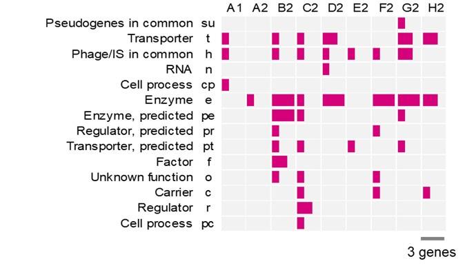
- I hope the authors can re-consider the title; "Diversity for commonality" does not make much sense to me. For example, it can be simply just "Diversity and commonality."
Thank you for the suggestion. The title was simplified as follows.
(L1) “Experimental evolution for the recovery of growth loss due to genome reduction.”
- It is not easy for me to locate and distinguish the RNA-seq vs DNA-seq files in DRA013662 at DDBJ. Could you make some notes on what RNA-seq actually are, vs what DNA-seq files actually are?
Sorry for the mistakes in the DRA number of DNA-seq. DNA-seq and RNA-seq were deposited separately with the accession IDs of DRA013661 and DRA013662, respectively. The following correction was made in the revision.
(L382-383) “The raw datasets of DNA-seq were deposited in the DDBJ Sequence Read Archive under the accession number DRA013661.”
-
-
www.biorxiv.org www.biorxiv.org
-
Author Response
The following is the authors’ response to the original reviews.
Reviewer #1 (Public Review):
Summary:
The authors aim to address a critical challenge in the field of bioinformatics: the accurate and efficient identification of protein binding sites from sequences. Their work seeks to overcome the limitations of current methods, which largely depend on multiple sequence alignments or experimental protein structures, by introducing GPSite, a multi-task network designed to predict binding residues of various molecules on proteins using ESMFold.
Strengths:
-
Benchmarking. The authors provide a comprehensive benchmark against multiple methods, showcasing the performances of a large number of methods in various scenarios.
-
Accessibility and Ease of Use. GPSite is highlighted as a freely accessible tool with user-friendly features on its website, enhancing its potential for widespread adoption in the research community.
RE: We thank the reviewer for acknowledging the contributions and strengths of our work!
Weaknesses:
- Lack of Novelty. The method primarily combines existing approaches and lacks significant technical innovation. This raises concerns about the original contribution of the work in terms of methodological development. Moreover, the paper reproduces results and analyses already presented in previous literature, without providing novel analysis or interpretation. This further diminishes the contribution of this paper to advancing knowledge in the field.
RE: The novelty of this work is primarily manifested in four key aspects. Firstly, although we have employed several existing tools such as ProtTrans and ESMFold to extract sequence features and predict protein conformations, these techniques were hardly explored in the field of binding site prediction. We have successfully demonstrated the feasibility of substituting multiple sequence alignments with language model embeddings and training with predicted structures, providing a new solution to overcome the limitations of current methods for genome-wide applications. Secondly, though a few methods tend to capture geometric information based on protein surfaces or atom graphs, surface calculation and property mapping are usually time-consuming, while massage passing on full atom graphs is memory-consuming and thus challenging to process long sequences. Besides, these methods are sensitive towards details and errors in the predicted structures. To facilitate large-scale annotations, we have innovatively applied geometric deep learning to protein residue graphs for comprehensively capturing backbone and sidechain geometric contexts in an efficient and effective manner (Figure 1). Thirdly, we have not only exploited multi-task learning to integrate diverse ligands and enhance performance, but also shown its capability to easily extend to the binding site prediction of other unseen ligands (Figure 4 D-E). Last but not least, as a “Tools and Resources” article, we have provided a fast, accurate and user-friendly webserver, as well as constructed a large annotation database for the sequences in Swiss-Prot. Leveraging this database, we have conducted extensive analyses on the associations between binding sites and molecular functions, biological processes, and disease-causing mutations (Figure 5), indicating the potential of our tool to unveil unexplored biology underlying genomic data.
We have now revised the descriptions in the “The geometry-aware protein binding site predictor (GPSite)” section to highlight the novelty of our work in a clearer manner:
“In conclusion, GPSite is distinguished from the previous approaches in four key aspects. First, profiting from the effectiveness and low computational cost of ProtTrans and ESMFold, GPSite is liberated from the reliance on MSA and native structures, thus enabling genome-wide binding site prediction. Second, unlike methods that only explore the Cα models of proteins 25,40, GPSite exploits a comprehensive geometric featurizer to fully refine knowledge in the backbone and sidechain atoms. Third, the employed message propagation on residue graphs is global structure-aware and time-efficient compared to the methods based on surface point clouds 21,22, and memory-efficient unlike methods based on full atom graphs 23,24. Residue-based message passing is also less sensitive towards errors in the predicted structures. Last but not least, instead of predicting binding sites for a single molecule type or learning binding patterns separately for different molecules, GPSite applies multi-task learning to better model the latent relationships among different binding partners.”
- Benchmark Discrepancies. The variation in benchmark results, especially between initial comparisons and those with PeSTo. GPSite achieves a PR AUC of 0.484 on the global benchmark but a PR AUC of 0.61 on the benchmark against PeSTo. For consistency, PeSTo should be included in the benchmark against all other methods. It suggests potential issues with the benchmark set or the stability of the method. This inconsistency needs to be addressed to validate the reliability of the results.
RE: We thank the reviewer for the constructive comments. Since our performance comparison experiments involved numerous competitive methods whose training sets are disparate, it was difficult to compare or rank all these methods fairly using a single test set. Given the substantial overlap between our protein-binding site test set and the training set of PeSTo, we meticulously re-split our entire protein-protein binding site dataset to generate a new test set that avoids any overlap with the training sets of both GPSite and PeSTo and performed a separate evaluation, where GPSite achieves a higher AUPR than PeSTo (0.610 against 0.433). This is quite common in this field. For instance, in the study of PeSTo (Nat Commun 2023), the comparisons of PeSTo with MaSIF-site, SPPIDER, and PSIVER were conducted using one test set, while the comparison with ScanNet was performed on a separate test set.
Based on the reviewer’s suggestion, we have now replaced this experiment with a direct comparison with PeSTo using the datasets from PeSTo, in order to enhance the completeness and convincingness of our results. The corresponding descriptions are now added in Appendix 1-note 2, and the results are added in Appendix 2-table 4. For convenience, we also attach the note and table here:
“Since 340 out of 375 proteins in our protein-protein binding site test set share > 30% identity with the training sequences of PeSTo, we performed a separate comparison between GPSite and PeSTo using the training and test datasets from PeSTo. By re-training with simply the same hyperparameters, GPSite achieves better performance than PeSTo (AUPR of 0.824 against 0.797) as shown in Appendix 2-table 4. Furthermore, when using ESMFold-predicted structures as input, the performance of PeSTo decreases substantially (AUPR of 0.691), and the superiority of our method will be further reflected. As in 24, the performance of ScanNet is also included (AUPR of 0.720), which is also largely outperformed by GPSite.”
Author response table 1.
Performance comparison of GPSite with ScanNet and PeSTo on the protein-protein binding site test set from PeSTo 24
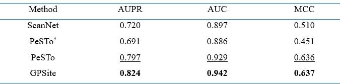
Note: The performance of ScanNet and PeSTo are directly obtained from 24. PeSTo* denotes evaluation using the ESMFold-predicted structures as input. The metrics provided are the median AUPR, median AUC and median MCC. The best/second-best results are indicated by bold/underlined fonts.
- Interface Definition Ambiguity. There is a lack of clarity in defining the interface for the binding site predictions. Different methods are trained using varying criteria (surfaces in MaSIF-site, distance thresholds in ScanNet). The authors do not adequately address how GPSite's definition aligns with or differs from these standards and how this issue was addressed. It could indicate that the comparison of those methods is unreliable and unfair.
RE: We thank the reviewer for the comments. The precise definition of ligand-binding sites is elucidated in the “Benchmark datasets” section. Specifically, the datasets of DNA, RNA, peptide, ATP, HEM and metal ions used to train GPSite were collected from the widely acknowledged BioLiP database [PMID: 23087378]. In BioLiP, a binding residue is defined if the smallest atomic distance between the target residue and the ligand is <0.5 Å plus the sum of the Van der Waal’s radius of the two nearest atoms. Meanwhile, most comparative methods regarding these ligands were also trained on data from BioLiP, thereby ensuring fair comparisons.
However, since BioLiP does not include data on protein-protein binding sites, studies for protein-protein binding site prediction may adopt slightly distinct label definitions, as the reviewer suggested. Here, we employed the protein-protein binding site data from our previous study [PMID: 34498061], where a protein-binding residue was defined as a surface residue (relative solvent accessibility > 5%) that lost more than 1 Å2 absolute solvent accessibility after protein-protein complex formation. This definition was initially introduced in PSIVER [PMID: 20529890] and widely applied in various studies (e.g., PMID: 31593229, PMID: 32840562). SPPIDER [PMID: 17152079] and MaSIF-site [PMID: 31819266] have also adopted similar surface-based definitions as PSIVER. On the other hand, ScanNet [PMID: 35637310] employed an atom distance threshold of 4 Å to define contacts while PeSTo [PMID: 37072397] used a threshold of 5 Å. However, it is noteworthy that current methods in this field including ScanNet (Nat Methods 2022) and PeSTo (Nat Commun 2023) directly compared methods using different label definitions without any alignment in their benchmark studies, likely due to the subtle distinctions among these definitions. For instance, the study of PeSTo directly performed comparisons with ScanNet, MaSIF-site, SPPIDER, and PSIVER. Therefore, we followed these previous works, directly comparing GPSite with other protein-protein binding site predictors.
In the revised “Benchmark datasets” section, we have now provided more details for the binding site definitions in different datasets to avoid any potential ambiguity:
“The benchmark datasets for evaluating binding site predictions of DNA, RNA, peptide, ATP, and HEM are constructed from BioLiP”; “A binding residue is defined if the smallest atomic distance between the target residue and the ligand is < 0.5 Å plus the sum of the Van der Waal’s radius of the two nearest atoms”; “Besides, the benchmark dataset of protein-protein binding sites is directly from 26, which contains non-redundant transient heterodimeric protein complexes dated up to May 2021. Surface regions that become solvent inaccessible on complex formation are defined as the ground truth protein-binding sites. The benchmark datasets of metal ion (Zn2+, Ca2+, Mg2+ and Mn2+) binding sites are directly from 18, which contain non-redundant proteins dated up to December 2021 from BioLiP.”
While GPSite demonstrates the potential to surpass state-of-the-art methods in protein binding site prediction, the evidence supporting these claims seems incomplete. The lack of methodological novelty and the unresolved questions in benchmark consistency and interface definition somewhat undermine the confidence in the results. Therefore, it's not entirely clear if the authors have fully achieved their aims as outlined.
The work is useful for the field, especially in disease mechanism elucidation and novel drug design. The availability of genome-scale binding residue annotations GPSite offers is a significant advancement. However, the utility of this tool could be hampered by the aforementioned weaknesses unless they are adequately addressed.
RE: We thank the reviewer for acknowledging the advancement and value of our work, as well as pointing out areas where improvements can be made. As discussed above, we have now carried out the corresponding revisions in the revised manuscript to enhance the completeness and clearness of our work.
Reviewer #2 (Public Review):
Summary:
This work provides a new framework, "GPsite" to predict DNA, RNA, peptide, protein, ATP, HEM, and metal ions binding sites on proteins. This framework comes with a webserver and a database of annotations. The core of the model is a Geometric featurizer neural network that predicts the binding sites of a protein. One major contribution of the authors is the fact that they feed this neural network with predicted structure from ESMFold for training and prediction (instead of native structure in similar works) and a high-quality protein Language Model representation. The other major contribution is that it provides the public with a new light framework to predict protein-ligand interactions for a broad range of ligands.
The authors have demonstrated the interest of their framework with mostly two techniques: ablation and benchmark.
Strengths:
-
The performance of this framework as well as the provided dataset and web server make it useful to conduct studies.
-
The ablations of some core elements of the method, such as the protein Language Model part, or the input structure are very insightful and can help convince the reader that every part of the framework is necessary. This could also guide further developments in the field. As such, the presentation of this part of the work can hold a more critical place in this work.
RE: We thank the reviewer for recognizing the contributions of our work and for noting that our experiments are thorough.
Weaknesses:
- Overall, we can acknowledge the important effort of the authors to compare their work to other similar frameworks. Yet, the lack of homogeneity of training methods and data from one work to the other makes the comparison slightly unconvincing, as the authors pointed out. Overall, the paper puts significant effort into convincing the reader that the method is beating the state of the art. Maybe, there are other aspects that could be more interesting to insist on (usability, interest in protein engineering, and theoretical works).
RE: We sincerely appreciate the reviewer for the constructive and insightful comments. As to the concern of training data heterogeneity raised by the reviewer, it is noteworthy that current studies in this field, such as ScanNet (Nat Methods 2022) and PeSTo (Nat Commun 2023), directly compare methods trained on different datasets in their benchmark experiments. Therefore, we have adhered to the paradigm in these previous works. According to the detailed recommendations by the reviewer, we have now improved our manuscript by incorporating additional ablation studies regarding the effects of training procedure and language model representations, as well as case studies regarding the predicted structure’s quality and GPSite-based function annotations. We have also refined the Discussion section to focus more on the achievements of this work. A comprehensive point-by-point response to the reviewer’s recommendations is provided below.
Reviewer #2 (Recommendations For The Authors):
Major comments:
Overall I think the work is slightly deserved by its presentation. Some improvements could be made to the paper to better highlight the significance of your contribution.
RE: We thank the reviewer for recognizing the significance of our work!
- Line 188: "As expected, the performance of these methods mostly decreases substantially utilizing predicted structures for testing because they were trained with high-quality native structures.
This is a major ablation that was not performed in this case. You used the predicted structure to train, while the other did not. One better way to assess the interest of this approach would be to compare the performance of a network trained with only native structure to compare the leap in performance with and without this predicted structure as you did after to assess the interest of some other aspect of your method such as single to multitask.
RE: We thank the reviewer for the valuable recommendation. We have now assessed the benefit of training with predicted instead of native structures, which brings an average AUPR increase of 4.2% as detailed in Appendix 1-note 5 and Appendix 2-table 9. For convenience, we also attach the note and table here:
“We examined the performance under different training and evaluation settings as shown in Appendix 2-table 9. As expected, the model yields exceptional performance (average AUPR of 0.656) when trained and evaluated using native structures. However, if this model is fed with predicted structures of the test proteins, the performance substantially declines to an average AUPR of 0.573. This trend aligns with the observations for other structure-based methods as illustrated in Figure 2. More importantly, in the practical scenario where only predicted structures are available for the target proteins, training the model with predicted structures (i.e., GPSite) results in superior performance than training the model with native structures (average AUPR of 0.594 against 0.573), probably owing to the consistency between the training and testing data. For completeness, the results in Appendix 3-figure 2 are also included where GPSite is tested with native structures (average AUPR of 0.637).”
Author response table 2.
Performance comparison on the ten binding site test sets under different training and evaluation settings
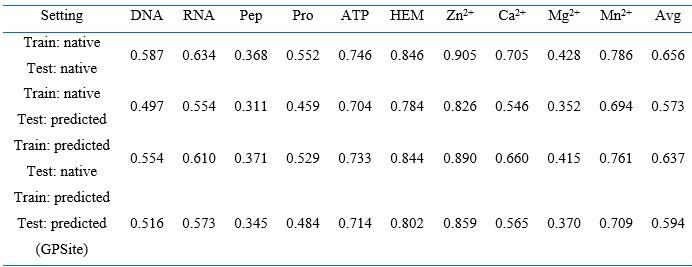
Note: The numbers in this table are AUPR values. “Pep” and “Pro” denote peptide and protein, respectively. “Avg” means the average AUPR values among the ten test sets. “native” and “predicted” denote applying native and predicted structures as input, respectively.
- Line 263: "ProtTrans consistently obtains competitive or superior performance compared to the MSA profiles, particularly for the target proteins with few homologous sequences (Neff < 2)."
This seems a bit far-fetched. If we see clearly in the figure that the performances are far superior for Neff < 2. The performances seem rather similar for higher Neff. Could the author evaluate numerically the significance of the improvement? MSA profiles outperform GPSite on 4 intervals and I don't know the distribution of the data.
RE: We thank the reviewer for the valuable suggestion. We have now revised this sentence to avoid any potential ambiguity:
“As evidenced in Figure 4B and Appendix 2-table 8, ProtTrans consistently obtains competitive or superior performance compared to the MSA profile. Notably, for the target proteins with few homologous sequences (Neff < 2), ProtTrans surpasses MSA profile significantly with an improvement of 3.9% on AUC (P-value = 4.3×10⁻⁸).”
The detailed significance tests and data distribution are now added in Appendix 2-table 8 and attached below as Author response-table 3 for convenience:
Author response table 3.
Performance comparison between GPSite and the baseline model using MSA profile for proteins with different Neff values in the combined test set of the ten ligands
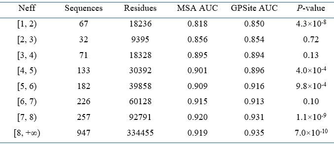
Note: Significance tests are performed following the procedure in 12,25. If P-value < 0.05, the difference between the performance is considered statistically significant.
- Line 285: "We first visualized the distributions of residues in this dataset using t-SNE, where the residues are encoded by raw feature vectors encompassing ProtTrans embeddings and DSSP structural properties, or latent embedding vectors from the shared network of GPSite. "
Wouldn't embedding from single-task be more relevant to show the interest of multi-task training here? Is the difference that big when comparing embeddings from single-task training to embeddings from multi-task training? Otherwise, I think the evidence from Figure 4e is sufficient, the interest of multitasking could be well-shown by single-task vs. multi-task AUPR and a few examples or predictions that are improved.
RE: We thank the reviewer for the comment. In the second paragraph of the “The effects of protein features and model designs” section, we have compared the performance of multi-task and single-task learning. However, the visualization results in Figure 4D are related to the third paragraph, where we conducted a downstream exploration of the possibility to extend GPSite to other unseen ligands. This is based on the hypothesis that the shared network in GPSite may have captured certain common ligand-binding mechanisms during the preceding multi-task training process. We visualized the distributions of residues in an unseen carbohydrate-binding site dataset using t-SNE, where the residues are encoded by raw feature vectors (ProtTrans and DSSP), or latent embedding vectors from the shared network trained before. Although the shared network has not been specifically trained on the carbohydrate dataset, the latent representations from GPSite effectively improve the discriminability between the binding and non-binding residues as shown in Figure 4D. This finding indicates that the shared network trained on the initial set of ten molecule types has captured common binding mechanisms and may be applied to other unseen ligands.
We have now added more descriptions in this paragraph to avoid potential ambiguity:
“Residues that are conserved during evolution, exposed to solvent, or inside a pocket-shaped domain are inclined to participate in ligand binding. During the preceding multi-task training process, the shared network in GPSite should have learned to capture such common binding mechanisms. Here we show how GPSite can be easily extended to the binding site prediction for other unseen ligands by adopting the pre-trained shared network as a feature extractor. We considered a carbohydrate-binding site dataset from 54 which contains 100 proteins for training and 49 for testing. We first visualized the distributions of residues in this dataset using t-SNE 55, where the residues are encoded by raw feature vectors encompassing ProtTrans embeddings and DSSP structural properties, or latent embedding vectors from the shared network of GPSite trained on the ten molecule types previously.”
- Line291: "Employing these informative hidden embeddings as input features to train a simple MLP exhibits remarkable performance with an AUC of 0.881 (Figure 4E), higher than that of training a single-task version of GPSite from scratch (AUC of 0.853) or other state-of-the-art methods such as MTDsite and SPRINT-CBH."
Is it necessary to introduce other methods here? The single-task vs multi-task seems enough for what you want to show?
RE: We thank the reviewer for the comment. As discussed above, here we aim to show the potential of GPSite for the binding site prediction of unseen ligand (i.e., carbohydrate) by adopting the pre-trained shared network as a feature extractor. Thus, we think it’s reasonable to also include the performance of other state-of-the-art methods in this carbohydrate benchmark dataset as baselines.
- Line 321: "Specifically, a protein-level binding score can be generated for each ligand by averaging the top k predicted scores among all residues. Empirically, we set k to 5 for metal ions and 10 for other ligands, considering that the binding interfaces of metal ions are usually smaller."
Since binding sites are usually not localized on one single amino-acid, we can expect that most of the top k residues are localized around the same area of the protein both spatially and along the sequence. Is it something you observe and could consider in your method?
RE: We thank the reviewer for the comment. We employed a straightforward method (top-k average) to convert GPSite’s residue-level annotations into protein-level annotations, where k was set empirically based on the distributions of the numbers of binding residues per sequence observed in the training set. We have not put much effort in optimizing this strategy since it mainly serves as a proof-of-concept experiment (Figure 5 A-C) to show the potential of GPSite in discriminating ligand-binding proteins. We have now revised this sentence to better explain how we selected k:
“Specifically, a protein-level binding score indicating the overall binding propensity to a specific ligand can be generated by averaging the top k predicted scores among all residues. Empirically, we set k to 5 for metal ions and 10 for other ligands, considering the distributions of the numbers of binding residues per sequence observed in the training set.”
As for the question raised by the reviewer, we can indeed expect that most of the top k predicted binding residues tend to cluster into several but not necessarily one area. For instance, certain macromolecules like DNA may interact with several protein surface patches due to their elongated structures (e.g., Author esponse-figure 1A). Another case may be a protein binding to multiple molecules of the same ligand type (e.g., Author response-figure 1B).
Author response image 1.
The structures of 4XQK (A) and 4KYW (B) in PDB.
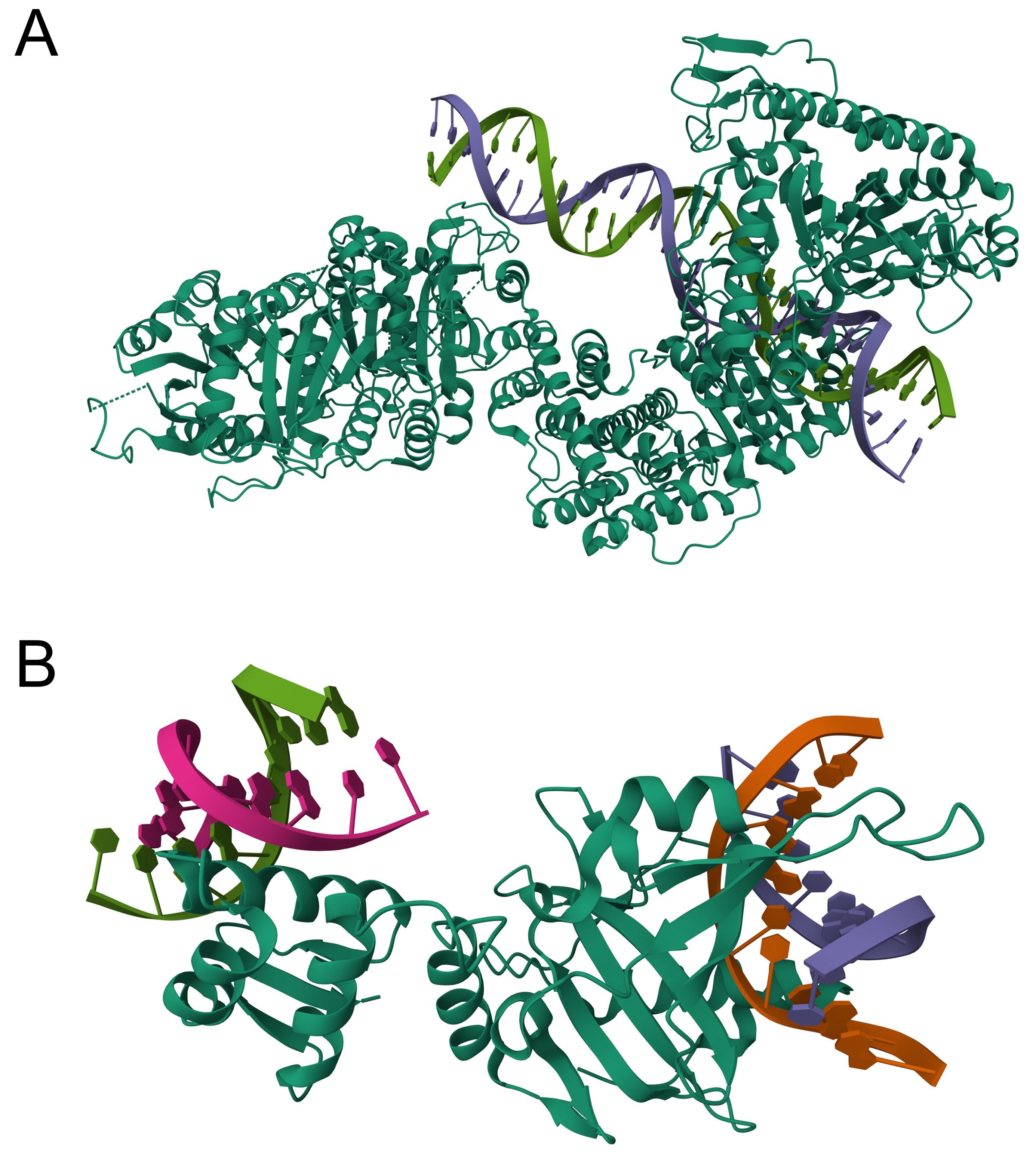
- Line 327: The accuracy of the GPSite protein-level binding scores is further validated by the ROC curves in Figure 5B, where GPSite achieves satisfactory AUC values for all ligands except protein (AUC of 0.608).
Here may be a good place to compare yourself with others, do other frameworks experience the same problem? If so, AUC and AUPR are not relevant here, can you expose some recall scores for example?
RE: We thank the reviewer for the valuable recommendation. We have conducted comprehensive method comparisons in the preceding “GPSite outperforms state-of-the-art methods” section, where GPSite surpasses all existing frameworks across various ligands. Here, the genome-wide analyses of Swiss-Prot in Figure 5 serve as a downstream demonstration of GPSite’s capacity for large-scale annotations. We didn’t compare with other methods since most of them are time-consuming or memory-consuming, thus unavailable to process sequences of substantial quantity or length. For example, it takes about 8 min for the MSA-based method GraphBind to annotate a protein with 500 residues, while it just takes about 20 s for GPSite (see Appendix 3-figure 1 for detailed runtime comparison). It is also challenging for the atom-graph-based method PeSTo to process structures more than 100 kDa (~1000 residues) on a 32 GB GPU as the authors suggested, while GPSite can easily process structures containing up to 2500 residues on a 16 GB GPU.
Regarding the recall score mentioned by the reviewer, GPSite achieves a recall of 0.95 (threshold = 0.5) for identifying protein-binding proteins. This indicates that GPSite can accurately identify positive samples, but it also tends to misclassify negative samples as positive. In our original manuscript, we claimed that “This may be ascribed to the fact that protein-protein interactions are ubiquitous in living organisms while the Swiss-Prot function annotations are incomplete”. To better support this claim, we have now added two examples in Appendix 1-note 7, where GPSite confidently predicted the presences of the “protein binding” function (GO:0005515). Notably, this function was absent in these two proteins in the Swiss-Prot database at the time of manuscript preparation (release: 2023-05-03), but has been included in the latest release of Swiss-Prot (release: 2023-11-08). For convenience, we also attach the note here:
“As depicted in Figure 5A, GPSite assigns relatively high prediction scores to the proteins without “protein binding” function in the Swiss-Prot annotations, leading to a modest AUC value of 0.608 (Figure 5B). This may be ascribed to the fact that protein-protein interactions are ubiquitous in living organisms while the Swiss-Prot function annotations are incomplete. To support this hypothesis, we present two proteins as case studies, both sharing < 20% sequence identity with the protein-binding training set of GPSite. The first case is Aminodeoxychorismate synthase component 2 from Escherichia coli (UniProt ID: P00903). GPSite confidently predicted this protein as a protein-binding protein with a high prediction score of 0.936. Notably, this protein was not annotated with the “protein binding” function (GO:0005515) or any of its GO child terms in the Swiss-Prot database at the time of manuscript preparation (https://rest.uniprot.org/unisave/P00903?format=txt&versions=171, release: 2023-05-03). However, in the latest release of Swiss-Prot (https://rest.uniprot.org/unisave/P00903?format=txt&versions=174, release: 2023-11-08) during manuscript revision, this protein is annotated with the “protein heterodimerization activity” function (GO:0046982), which is a child term of “protein binding”. In fact, the heterodimerization activity of this protein has been validated through experiments in the year of 1996 (PMID: 8679677), indicating the potential incompleteness of the Swiss-Prot annotations. The other case is Hydrogenase-2 operon protein HybE from Escherichia coli (UniProt ID: P0AAN1), which was also predicted as a protein-binding protein by GPSite (score = 0.909). Similarly, this protein was not annotated with the “protein binding” function in the Swiss-Prot database at the time of manuscript preparation (https://rest.uniprot.org/unisave/P0AAN1?format=txt&versions=108). However, in the latest release of Swiss-Prot (https://rest.uniprot.org/unisave/P0AAN1?format=txt&versions=111), this protein is annotated with the “preprotein binding” function (GO:0070678), which is a child term of “protein binding”. In fact, the preprotein binding function of this protein has been validated through experiments in the year of 2003 (PMID: 12914940). These cases demonstrate the effectiveness of GPSite for completing the missing function annotations in Swiss-Prot.”
- Line 381: 'Despite the noteworthy advancements achieved by GPSite, there remains scope for further improvements. Given that the ESM Metagenomic Atlas 34 provides 772 million predicted protein structures along with pre-computed language model embeddings, self-supervised learning can be employed to train a GPSite model for predicting masked sequence and structure attributes, or maximizing the similarity between the learned representations of substructures from identical proteins while minimizing the similarity between those from different proteins using a contrastive loss function training from scratch. Additional opportunities for upgrade exist within the network architecture. For example, a variational Expectation-Maximization (EM) framework 58 can be adopted to handle the hierarchical graph structure inherent in proteins, which contains the top view of the residue graph and the bottom view of the atom graph inside a residue. Such an EM procedure enables training two separate graph neural networks for the two views while simultaneously allowing interaction and mutual enhancement between the two modules. Meta-learning could also be explored in this multi-task scenario, which allows fast adaptation to unseen tasks with limited labels.'
I think this does not belong here. It feels like half of your discussion is not talking about the achievements of this paper but future very specific directions. Focus on the take-home arguments (performances of the model, ability to predict a large range of tasks, interest in key components of your model, easy use) of the paper and possible future direction but without being so specific.
RE: We thank the reviewer for the valuable suggestion. We have now simplified the discussions on the future directions notably:
“Despite the noteworthy advancements achieved by GPSite, there remains scope for further improvements. GPSite may be improved by pre-training on the abundant predicted structures in ESM Metagenomic Atlas, and then fine-tuning on binding site datasets. Besides, the hidden embeddings from ESMFold may also serve as informative protein representations. Additional opportunities for upgrade exist within the network architecture. For example, a variational Expectation-Maximization framework can be adopted to handle the hierarchical atom-to-residue graph structure inherent in proteins. Meta-learning could also be explored in this multi-task scenario, which allows fast adaptation to unseen tasks with limited labels.”
- Overall there is also a lack of displayed structure. You should try to select a few examples of binding sites that were identified correctly by your method and not by others, if possible get some insights on why. Also, some negative examples could be interesting so as to have a better idea of the interest.
RE: We thank the reviewer for the valuable recommendation. We have performed a case study for the structure of the glucocorticoid receptor in Figure 3 D-H to illustrate a potential reason for the robustness of GPSite. Moreover, we have now added a case study in Appendix 1-note 3 and Appendix 3-figure 5 to explain why GPSite sometimes is not as accurate as the state-of-the-art structure-based method. For convenience, we also attach the note and figure here:
“Here we present an example of an RNA-binding protein, i.e., the ribosome biogenesis protein ERB1 (PDB: 7R6Q, chain m), to illustrate the impact of predicted structure’s quality. As shown in Appendix 3-figure 5, ERB1 is an integral component of a large multimer structure comprising protein and RNA chains (i.e., the state E2 nucleolar 60S ribosome biogenesis intermediate). Likely due to the neglect of interactions from other protein chains, ESMFold fails to predict the correct conformation of the ERB1 chain (TM-score = 0.24). Using this incorrect predicted structure, GPSite achieves an AUPR of 0.580, lower than GraphBind input with the native structure (AUPR = 0.636). However, the performance of GraphBind substantially declines to an AUPR of 0.468 when employing the predicted structure as input. Moreover, if GPSite adopts the native structure for prediction, a notable performance boost can be obtained (AUPR = 0.681).”
Author response image 2.
The prediction results of GPSite and GraphBind for the ribosome biogenesis protein ERB1. (A) The state E2 nucleolar 60S ribosome biogenesis intermediate (PDB: 7R6Q). The ribosome biogenesis protein ERB1 (chain m) is highlighted in blue, while other protein chains are colored in gray. The RNA chains are shown in orange. (B) The RNA-binding sites on ERB1 (colored in red). (C) The ESMFold-predicted structure of ERB1 (TM-score = 0.24). The RNA-binding sites are also mapped onto this predicted structure (colored in red). (D-G) The prediction results of GPSite and GraphBind for the predicted and native ERB1 structures. The confidence of the predictions is represented with a gradient of color from blue for non-binding to red for binding.
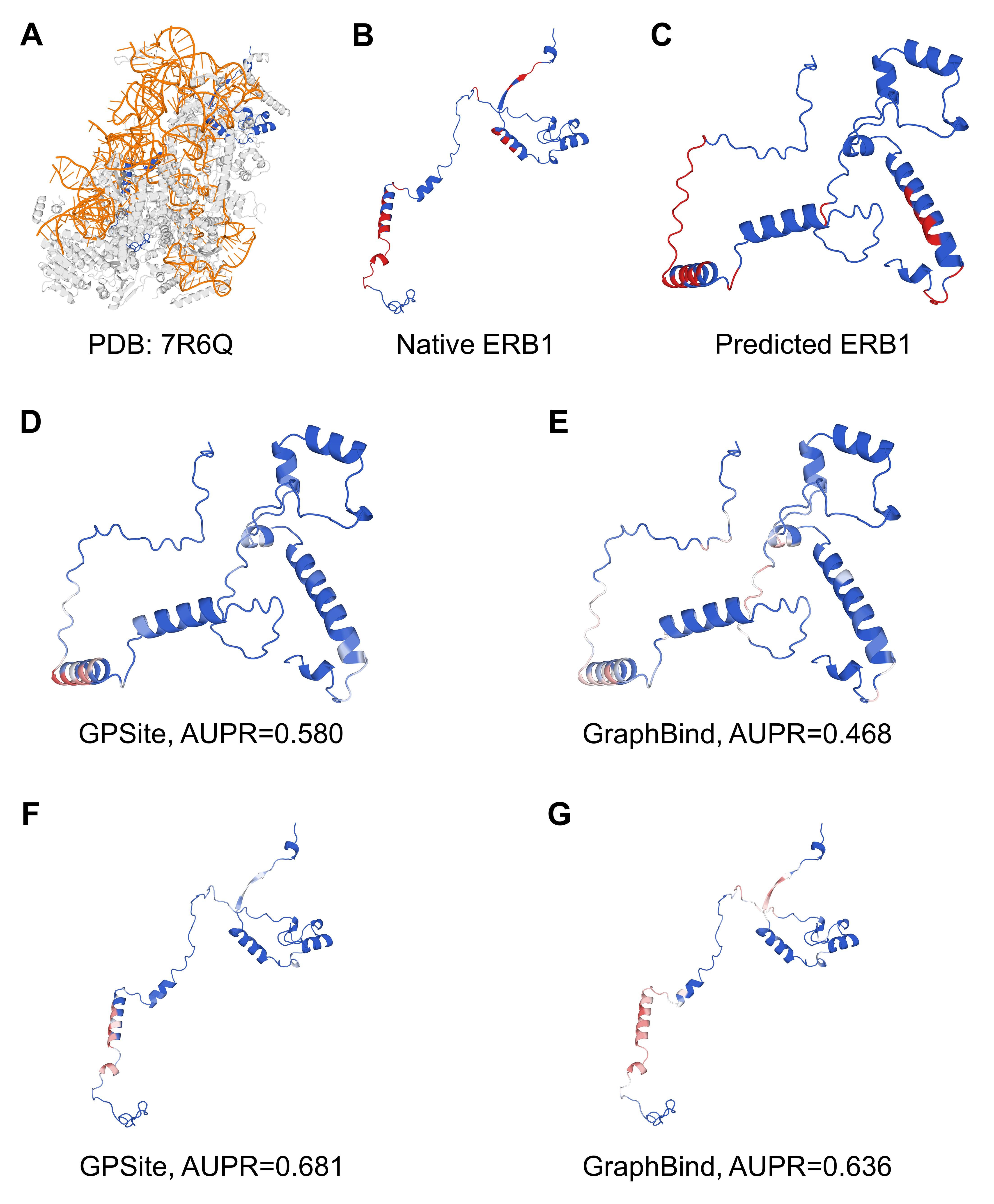
Minor comments:
- Line 169: "Note that since our test sets may partly overlap with the training sets of these methods, the results reported here should be the upper limits for the existing methods."
Yes, but they were potentially not trained on the most recent structures in that case. These methods could also see improved performance with an updated training set.
RE: We thank the reviewer for the comment. We have now deleted this sentence.
- Line176: "Since 358 of the 375 proteins in our protein-binding site test set share > 30% identity with the training sequences of PeSTo, we re-split our protein-binding dataset to generate a test set of 65 proteins sharing < 30% identity with the training set of PeSTo for a fair evaluation."
Too specific to be here in my opinion.
RE: We thank the reviewer for the comment. We have now moved these details to Appendix 1-note 2. The description in the main text here is now more concise:
“Given the substantial overlap between our protein-binding site test set and the training set of PeSTo, we conducted separate training and comparison using the datasets of PeSTo, where GPSite still demonstrates a remarkable improvement over PeSTo (Appendix 1-note 2).”
- Figure 2. The authors should try to either increase Fig A's size or increase the font size. This could probably be done by compressing the size of Figure C into a single figure.
RE: We thank the reviewer for the suggestion. We have now increased the font size in Figure A. Besides, the figures in the final version of the manuscript should be clearer where we could upload SVG files.
- Have you tried using embeddings from more structure-aware pLM such as ESM Fold embeddings (fine-tuned) or ProstTrans (that may be more recent than this study)?
RE: We thank the reviewer for the insightful comment. We have not yet explored the embeddings from structure-aware pLM, but we acknowledge its potential as a promising avenue for future investigation. We have now added this point in our Discussion section:
“Besides, the hidden embeddings from ESMFold may also serve as informative protein representations.”
Reviewer #3 (Public Review):
Summary
The authors of this work aim to address the challenge of accurately and efficiently identifying protein binding sites from sequences. They recognize that the limitations of current methods, including reliance on multiple sequence alignments or experimental protein structure, and the under-explored geometry of the structure, which limit the performance and genome-scale applications. The authors have developed a multi-task network called GPSite that predicts binding residues for a range of biologically relevant molecules, including DNA, RNA, peptides, proteins, ATP, HEM, and metal ions, using a combination of sequence embeddings from protein language models and ESMFold-predicted structures. Their approach attempts to extract residual and relational geometric contexts in an end-to-end manner, surpassing current sequence-based and structure-based methods.
Strengths
-
The GPSite model's ability to predict binding sites for a wide variety of molecules, including DNA, RNA, peptides, and various metal ions.
-
Based on the presented results, GPSite outperforms state-of-the-art methods in several benchmark datasets.
-
GPSite adopts predicted structures instead of native structures as input, enabling the model to be applied to a wider range of scenarios where native structures are rare.
-
The authors emphasize the low computational cost of GPSite, which enables rapid genome-scale binding residue annotations, indicating the model's potential for large-scale applications.
RE: We thank the reviewer for recognizing the significance and value of our work!
Weaknesses
- One major advantage of GPSite, as claimed by the authors, is its efficiency. Although the manuscript mentioned that the inference takes about 5 hours for all datasets, it remains unclear how much improvement GPSite can offer compared with existing methods. A more detailed benchmark comparison of running time against other methods is recommended (including the running time of different components, since some methods like GPSite use predicted structures while some use native structures).
RE: We thank the reviewer for the valuable suggestion. Empirically, it takes about 5-20 min for existing MSA-based methods to make predictions for a protein with 500 residues, while it only takes about 1 min for GPSite (including structure prediction). However, it is worth noting that some predictors in our benchmark study are solely available as webservers, and it is challenging to compare the runtime between a standalone program and a webserver due to the disparity in hardware configurations. Therefore, we have now included comprehensive runtime comparisons between the GPSite webserver and other top-performing servers in Appendix 3-figure 1 to illustrate the practicality and efficiency of our method. For convenience, we also attach the figure here as Author response-figure 3. The corresponding description is now added in the “GPSite outperforms state-of-the-art methods” section:
“Moreover, GPSite is computationally efficient, achieving comparable or faster prediction speed compared to other top-performing methods (Appendix 3-figure 1).”
Author response image 3.
Runtime comparison of the GPSite webserver with other top-performing servers. Five protein chains (i.e., 8HN4_B, 8USJ_A, 8C1U_A, 8K3V_A and 8EXO_A) comprising 100, 300, 500, 700, and 900 residues, respectively, were selected for testing, and the average runtime is reported for each method. Note that a significant portion of GPSite’s runtime (75 s, indicated in orange) is allocated to structure prediction using ESMFold.
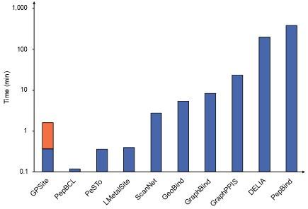
- Since the model uses predicted protein structure, the authors have conducted some studies on the effect of the predicted structure's quality. However, only the 0.7 threshold was used. A more comprehensive analysis with several different thresholds is recommended.
RE: We thank the reviewer for the comment. We assessed the effect of the predicted structure's quality by evaluating GPSite’s performance on high-quality (TM-score > 0.7) and low-quality (TM-score ≤ 0.7) predicted structures. We did not employ multiple thresholds (e.g., 0.3, 0.5, and 0.7), as the majority of proteins in the test sets were accurately predicted by ESMFold. Specifically, as shown in Figure 3B, Appendix 3-figure 3 and Appendix 2-table 5, the numbers of proteins with TM-score ≤ 0.7 are small in most datasets (e.g., 42 for DNA and 17 for ATP). Consequently, there is insufficient data available for analysis with lower thresholds, except for the RNA test set. Notably, Figure 3C presents a detailed inspection of the 104 proteins with TM-score < 0.5 in the RNA test set. Within this subset, GPSite consistently outperforms the state-of-the-art structure-based method GraphBind with predicted structures as input, regardless of the prediction quality of ESMFold. Only in cases where structures are predicted with extremely low quality (TM-score < 0.3) does GPSite fall behind GraphBind input with native structures. This result further demonstrates the robustness of GPSite. We have now added clearer explanations in the “GPSite is robust for low-quality predicted structures” section:
“Figure 3B and Appendix 3-figure 3 show the distributions of TM-scores between native and predicted structures calculated by US-align in the ten benchmark datasets, where most proteins are accurately predicted with TM-score > 0.7 (see also Appendix 2-table 5)”; “Given the infrequency of low-quality predicted structures except for the RNA test set, we took a closer inspection of the 104 proteins with predicted structures of TM-score < 0.5 in the RNA test set.”
- To demonstrate the robustness of GPSite, the authors performed a case study on human GR containing two zinc fingers, where the predicted structure is not perfect. The analysis could benefit from more a detailed explanation of why the model can still infer the binding site correctly even though the input structural information is slightly off.
RE: We thank the reviewer for the comment. We have actually explained the potential reason for the robustness of GPSite in the second paragraph of the “GPSite is robust for low-quality predicted structures” section. In summary, although the whole structure of this protein is not perfectly predicted, the local structures of the binding domains of peptide, DNA and Zn2+ are actually predicted accurately as evidenced by the superpositions of the native and predicted structures in Figure 3D and 3E. Therefore, GPSite can still make reliable predictions. We have now revised this paragraph to explain these more clearly:
“Figure 3D shows the structure of the human glucocorticoid receptor (GR), a transcription factor that binds DNA and assembles a coactivator peptide to regulate gene transcription (PDB: 7PRW, chain A). The DNA-binding domain of GR also consists of two C4-type zinc fingers to bind Zn2+ ions. Although the structure of this protein is not perfectly predicted (TM-score = 0.72), the local structures of the binding domains of peptide and DNA are actually predicted accurately as viewed by the superpositions of the native and predicted structures in Figure 3D and 3E. Therefore, GPSite can correctly predict all Zn2+ binding sites and precisely identify the binding sites of DNA and peptide with AUPR values of 0.949 and 0.924, respectively (Figure 3F, G and H).”
- To analyze the relatively low AUC value for protein-protein interactions, the authors claimed that it is "due to the fact that protein-protein interactions are ubiquitous in living organisms while the Swiss-Prot function annotations are incomplete", which is unjustified. It is highly recommended to support this claim by showing at least one example where GPSite's prediction is a valid binding site that is not present in the current Swiss-Prot database or via other approaches.
RE: We thank the reviewer for the valuable recommendation. To support this claim, we have now added two examples in Appendix 1-note 7, where GPSite confidently predicted the presences of the “protein binding” function (GO:0005515). Notably, this function was absent in these two proteins in the Swiss-Prot database at the time of manuscript preparation (release: 2023-05-03), but has been included in the latest release of Swiss-Prot (release: 2023-11-08). For convenience, we also attach the note below:
“As depicted in Figure 5A, GPSite assigns relatively high prediction scores to the proteins without “protein binding” function in the Swiss-Prot annotations, leading to a modest AUC value of 0.608 (Figure 5B). This may be ascribed to the fact that protein-protein interactions are ubiquitous in living organisms while the Swiss-Prot function annotations are incomplete. To support this hypothesis, we present two proteins as case studies, both sharing < 20% sequence identity with the protein-binding training set of GPSite. The first case is Aminodeoxychorismate synthase component 2 from Escherichia coli (UniProt ID: P00903). GPSite confidently predicted this protein as a protein-binding protein with a high prediction score of 0.936. Notably, this protein was not annotated with the “protein binding” function (GO:0005515) or any of its GO child terms in the Swiss-Prot database at the time of manuscript preparation (https://rest.uniprot.org/unisave/P00903?format=txt&versions=171, release: 2023-05-03). However, in the latest release of Swiss-Prot (https://rest.uniprot.org/unisave/P00903?format=txt&versions=174, release: 2023-11-08) during manuscript revision, this protein is annotated with the “protein heterodimerization activity” function (GO:0046982), which is a child term of “protein binding”. In fact, the heterodimerization activity of this protein has been validated through experiments in the year of 1996 (PMID: 8679677), indicating the potential incompleteness of the Swiss-Prot annotations. The other case is Hydrogenase-2 operon protein HybE from Escherichia coli (UniProt ID: P0AAN1), which was also predicted as a protein-binding protein by GPSite (score = 0.909). Similarly, this protein was not annotated with the “protein binding” function in the Swiss-Prot database at the time of manuscript preparation (https://rest.uniprot.org/unisave/P0AAN1?format=txt&versions=108). However, in the latest release of Swiss-Prot (https://rest.uniprot.org/unisave/P0AAN1?format=txt&versions=111), this protein is annotated with the “preprotein binding” function (GO:0070678), which is a child term of “protein binding”. In fact, the preprotein binding function of this protein has been validated through experiments in the year of 2003 (PMID: 12914940). These cases demonstrate the effectiveness of GPSite for completing the missing function annotations in Swiss-Prot.”
- The authors reported that many GPSite-predicted binding sites are associated with known biological functions. Notably, for RNA-binding sites, there is a significantly higher proportion of translation-related binding sites. The analysis could benefit from a further investigation into this observation, such as the analyzing the percentage of such interactions in the training site. In addition, if there is sufficient data, it would also be interesting to see the cross-interaction-type performance of the proposed model, e.g., train the model on a dataset excluding specific binding sites and test its performance on that class of interactions.
RE: We thank the reviewer for the suggestion. We would like to clarify that the analysis in Figure 5C was conducted at “protein-level” instead of “residue-level”. As described in the second paragraph of the “Large-scale binding site annotation for Swiss-Prot” section, a protein-level ligand-binding score was assigned to a protein by averaging the top k residue-level predicted binding scores. This protein-level score indicates the overall binding propensity of the protein to a specific ligand. We gathered the top 20,000 proteins with the highest protein-level binding scores for each ligand and found that their biological process annotations from Swiss-Prot were consistent with existing knowledge. We have now revised the corresponding sentence to explain these more clearly:
“Exploiting the residue-level binding site annotations, we could readily extend GPSite to discriminate between binding and non-binding proteins of various ligands. Specifically, a protein-level binding score indicating the overall binding propensity to a specific ligand can be generated by averaging the top k predicted scores among all residues.”
As for the cross-interaction-type performance raised by the reviewer, we have now conducted cross-type evaluations to investigate the specificity of the ligand-specific MLPs and the inherent similarities among different ligands in Appendix 1-note 6 and Appendix 2-table 10. For convenience, we also attach the note and table here:
“We conducted cross-type evaluations by applying different ligand-specific MLPs in GPSite for the test sets of different ligands. As shown in Appendix 2-table 10, for each ligand-binding site test set, the corresponding ligand-specific network consistently achieves the best performance. This indicates that the ligand-specific MLPs have specifically learned the binding patterns of particular molecules. We also noticed that the cross-type performance is reasonable for the ligands sharing similar properties. For instance, the DNA-specific MLP exhibits a reasonable AUPR when predicting RNA-binding sites, and vice versa. Similar trends are also observed between peptide and protein, as well as among metal ions as expected. Interestingly, the cross-type performance between ATP and HEM is also acceptable, potentially attributed to their comparable molecular weights (507.2 and 616.5, respectively).”
Author response table 4.
Cross-type performance by applying different ligand-specific MLPs in GPSite for the test sets of different ligands
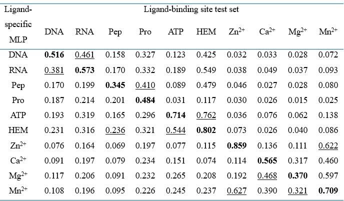
Note: “Pep” and “Pro” denote peptide and protein, respectively. The numbers in this table are AUPR values. The best/second-best result in each test set is indicated by bold/underlined font.
-
-
-
www.biorxiv.org www.biorxiv.org
-
Author response:
The following is the authors’ response to the original reviews
Public Reviews:
Reviewer #1 (Public review):
This work provides a new Python toolkit for combining generative modeling of neural dynamics and inversion methods to infer likely model parameters that explain empirical neuroimaging data. The authors provided tests to show the toolkit's broad applicability and accuracy; hence, it will be very useful for people interested in using computational approaches to better understand the brain.
Strengths:
The work's primary strength is the tool's integrative nature, which seamlessly combines forward modelling with backward inference. This is important as available tools in the literature can only do one and not the other, which limits their accessibility to neuroscientists with limited computational expertise. Another strength of the paper is the demonstration of how the tool can be applied to a broad range of computational models popularly used in the field to interrogate diverse neuroimaging data, ensuring that the methodology is not optimal to only one model. Moreover, through extensive in-silico testing, the work provided evidence that the tool can accurately infer ground-truth parameters, which is important to ensure results from future hypothesis testing are meaningful.
We are happy to hear the positive feedback on our effort to provide an open-source and widely accessible tool for both fast forward simulations and flexible model inversion, applicable across popular models of large-scale brain dynamics.
Weaknesses:
Although the tool itself is the main strength of the work, the paper lacked a thorough analysis of issues concerning robustness and benchmarking relative to existing tools.
The first issue is the robustness to the choice of features to be included in the objective function. This choice significantly affects the training and changes the results, as the authors even acknowledged themselves multiple times (e.g., Page 17 last sentence of first paragraph or Page 19 first sentence of second paragraph). This brings the question of whether the accurate results found in the various demonstrations are due to the biased selection of features (possibly from priors on what worked in previous works). The robustness of the neural estimator and the inference method to noise was also not demonstrated. This is important as most neuroimaging measurements are inherently noisy to various degrees.
The second issue is on benchmarking. Because the tool developed is, in principle, only a combination of existing tools specific to modeling or Bayesian inference, the work failed to provide a more compelling demonstration of its added value. This could have been demonstrated through appropriate benchmarking relative to existing methodologies, specifically in terms of accuracy and computational efficiency.
We fully agree with the reviewer that the VBI estimation heavily depends on the choice of data features, and this is the core of the inference procedure, not its weakness. We have demonstrated different scenarios showing how the informativeness of features (commonly used in the literature) results in varying uncertainty quantification. For instance, using summary statistics of functional connectivity (FC) and functional connectivity dynamics (FCD) matrices to estimate global coupling parameter leads to fast convergence; however, it is not sufficient to accurately estimate the whole-brain heterogeneous excitability parameter, which requires features such as statistical moments of time series. VBI provides a taxonomy of data features that users can employ to test their hypotheses. It is important to note that one major advantage of VBI is its ability to make estimation using a battery of data features, rather than relying on a limited set (such as only FC or FCD) as is often the case in the literature. In the revised version, we will elaborate further by presenting additional scenarios to demonstrate the robustness of the estimation. We will also evaluate the robustness of the neural density estimators to (dynamical/additive) noise.
More importantly, relative to benchmarking, we would like to draw attention to a key point regarding existing tools and methods. The literature often uses optimization for fitting whole-brain network models, and its limitations for reliable causal hypothesis testing have been pointed out in the Introduction/Discussion. As also noted by the reviewer under strengths, and to the best of our knowledge, there are no existing tools other than VBI that can scale and generalize to operate across whole-brain models for Bayesian model inversion. Previously, we developed Hamiltonian Monte Carlo (HMC) sampling for Epileptor model in epilepsy (Hashemi et al., 2020, Jha et al., 2022). This phenomenological model is very well-behaved in terms of numerical integration, gradient calculation, and dynamical system properties (Jirsa et al., 2014). However, this does not directly generalize to other models, particularly the Montbrió model for resting-state, which exhibits bistability with noise driving transitions between states. As shown in Baldy et al., 2024, even at the level of a single neural mass model (i.e., one brain region), gradient-based HMC failed to capture such switching behaviour, particularly when only one state variable (membrane potential) was observed while the other (firing rate) was missing. Our attempts to use other methods (e.g., the second-derivative-based Laplace approximation used in Dynamic Causal Modeling) also failed, due to divergence in gradient calculation. Nevertheless, reparameterization techniques (Baldy et al., 2024) and hybrid algorithms (Gabrié et al., 2022) could offer improvements, although this remains an open problem for these classes of computational models.
In sum, for oscillatory systems, it has been shown previously that SBI approach used in VBI substantially outperforms both gradient-based and gradient-free alternative methods (Gonçalves et al., 2020, Hashemi et al., 2023, Baldy et al., 2024). Importantly, for bistable systems with switching dynamics, gradient-based methods fail to converge, while gradient-free methods do not scale to the whole-brain level (Hashemi et al., 2020). Hence, the generalizability of VBI relies on the fact that neither the model nor the data features need to be differentiable. We will clarify this point in the revised version. Moreover, we will provide better explanations for some terms mentioned by the reviewer in Recommendations.
Hashemi, M., Vattikonda, A. N., Sip, V., Guye, M., Bartolomei, F., Woodman, M. M., & Jirsa, V. K. (2020). The Bayesian Virtual Epileptic Patient: A probabilistic framework designed to infer the spatial map of epileptogenicity in a personalized large-scale brain model of epilepsy spread. NeuroImage, 217, 116839.
Jha, J., Hashemi, M., Vattikonda, A. N., Wang, H., & Jirsa, V. (2022). Fully Bayesian estimation of virtual brain parameters with self-tuning Hamiltonian Monte Carlo. Machine Learning: Science and Technology, 3(3), 035016.
Jirsa, V. K., Stacey, W. C., Quilichini, P. P., Ivanov, A. I., & Bernard, C. (2014). On the nature of seizure dynamics. Brain, 137(8), 2210-2230.
Baldy, N., Breyton, M., Woodman, M. M., Jirsa, V. K., & Hashemi, M. (2024). Inference on the macroscopic dynamics of spiking neurons. Neural Computation, 36(10), 2030-2072.
Baldy, N., Woodman, M., Jirsa, V., & Hashemi, M. (2024). Dynamic Causal Modeling in Probabilistic Programming Languages. bioRxiv, 2024-11.
Gabrié, M., Rotskoff, G. M., & Vanden-Eijnden, E. (2022). Adaptive Monte Carlo augmented with normalizing flows. Proceedings of the National Academy of Sciences, 119(10), e2109420119.
Gonçalves, P. J., Lueckmann, J. M., Deistler, M., Nonnenmacher, M., Öcal, K., Bassetto, G., ... & Macke, J. H. (2020). Training deep neural density estimators to identify mechanistic models of neural dynamics. elife, 9, e56261.
Hashemi, M., Vattikonda, A. N., Jha, J., Sip, V., Woodman, M. M., Bartolomei, F., & Jirsa, V. K. (2023). Amortized Bayesian inference on generative dynamical network models of epilepsy using deep neural density estimators. Neural Networks, 163, 178-194.
Reviewer #2 (Public review):
Summary:
Whole-brain network modeling is a common type of dynamical systems-based method to create individualized models of brain activity incorporating subject-specific structural connectome inferred from diffusion imaging data. This type of model has often been used to infer biophysical parameters of the individual brain that cannot be directly measured using neuroimaging but may be relevant to specific cognitive functions or diseases. Here, Ziaeemehr et al introduce a new toolkit, named "Virtual Brain Inference" (VBI), offering a new computational approach for estimating these parameters using Bayesian inference powered by artificial neural networks. The basic idea is to use simulated data, given known parameters, to train artificial neural networks to solve the inverse problem, namely, to infer the posterior distribution over the parameter space given data-derived features. The authors have demonstrated the utility of the toolkit using simulated data from several commonly used whole-brain network models in case studies.
Strengths:
(1) Model inversion is an important problem in whole-brain network modeling. The toolkit presents a significant methodological step up from common practices, with the potential to broadly impact how the community infers model parameters.
(2) Notably, the method allows the estimation of the posterior distribution of parameters instead of a point estimation, which provides information about the uncertainty of the estimation, which is generally lacking in existing methods.
(3) The case studies were able to demonstrate the detection of degeneracy in the parameters, which is important. Degeneracy is quite common in this type of model. If not handled mindfully, they may lead to spurious or stable parameter estimation. Thus, the toolkit can potentially be used to improve feature selection or to simply indicate the uncertainty.
(4) In principle, the posterior distribution can be directly computed given new data without doing any additional simulation, which could improve the efficiency of parameter inference on the artificial neural network if well-trained.
We thank the reviewer for the careful consideration of important aspects of the VBI tool, such as uncertainty quantification, degeneracy detection, parallelization, and amortization strategy.
Weaknesses:
(1) While the posterior estimator was trained with a large quantity of simulated data, the testing/validation is only demonstrated with a single case study (one point in parameter space) per model. This is not sufficient to demonstrate the method's accuracy and reliability, but only its feasibility. Demonstrating the accuracy and reliability of the posterior estimation in large test sets would inspire more confidence.
(2) The authors have only demonstrated validation of the method using simulated data, but not features derived from actual EEG/MEG or fMRI data. So, it is unclear if the posterior estimator, when applied to real data, would produce results as sensible as using simulated data. Human data can often look quite different from the simulated data, which may be considered out of distribution. Thus, the authors should consider using simulated test data with out-of-distribution parameters to validate the method and using real human data to demonstrate, e.g., the reliability of the method across sessions.
(3) The z-scores used to measure prediction error are generally between 1-3, which seems quite large to me. It would give readers a better sense of the utility of the method if comparisons to simpler methods, such as k-nearest neighbor methods, are provided in terms of accuracy.
(4) A lot of simulations are required to train the posterior estimator, which seems much more than existing approaches. Inferring from Figure S1, at the required order of magnitudes of the number of simulations, the simulation time could range from days to years, depending on the hardware. Although once the estimator is well-trained, the parameter inverse given new data will be very fast, it is not clear to me how often such use cases would be encountered. Because the estimator is trained based on an individual connectome, it can only be used to do parameter inversion for the same subject. Typically, we only have one session of resting state data from each participant, while longitudinal resting state data where we can assume the structural connectome remains constant, is rare. Thus, the cost-efficiency and practical utility of training such a posterior estimator remains unclear.
We agree with the reviewer that it is necessary to show results on larger synthetic test sets, and we will elaborate further by presenting additional scenarios to demonstrate the robustness of the estimation. However, there are some points raised by the reviewer that we need to clarify.
The validation on empirical data was beyond the scope of this study, as it relates to model validation rather than the inversion algorithms. This is also because we aimed to avoid repetition, given that we have previously demonstrated model validation on empirical data using theses techniques, for invasive sEEG (Hashemi et al., 2023), MEG (Sorrentino et al., 2024), EEG (Angiolelli et al., 2025) and fMRI (Lavanga et al., 2024, Rabuffo et al., 2025). Note that if the features of the observed data are not included during training, VBI ignores them, as it requires an invertible mapping function between parameters and data features.
We have used z-scores and posterior shrinkage to measure prediction performance, as these are Bayesian metrics that take into account the variance of both prior and posterior rather than only the mean value or thresholding for ranking of the prediction used in k-NN or confusion matrix methods. This helps avoid biased accuracy estimation, for instance, if the mean posterior is close to the true value but there is no posterior shrinkage. Although shrinkage is bounded between 0 and 1, we agree that z-scores have no upper bound for such diagnostics.
Finally, the number of required simulations depends on the dimensionality of the parameter space and the informativeness of the data features. For instance, estimating a single global scaling parameter requires around 100 simulations, whereas estimating whole-brain heterogeneous parameters requires substantially more simulations. Nevertheless, we have provided fast simulations, and one key advantage of VBI is that simulations can be run in parallel (unlike MCMC sampling, which is more limited in this regard). Hence, with commonly accessible CPUs/GPUs, the fast simulations and parallelization capabilities of the VBI tool allow us to run on the order of 1 million simulations within 2–3 days on desktops, or in less than half a day on supercomputers at cohort level, rather than over several years! It has been previously shown that the SBI method used in VBI provides an order-of-magnitude faster inversion than HMC for whole-brain epilepsy spread (Hashemi et al., 2023). Moreover, after training, the amortized strategy is critical for enabling hypothesis testing within seconds to minutes. We agree that longitudinal resting-state data under the assumption of a constant structural connectome is rare; however, this strategy is essential in brain diseases such as epilepsy, where experimental hypothesis testing is prohibitive.
We will clarify these points and better explain some terms mentioned by the reviewer in the revised manuscript.
Hashemi, M., Vattikonda, A. N., Jha, J., Sip, V., Woodman, M. M., Bartolomei, F., & Jirsa, V. K. (2023). Amortized Bayesian inference on generative dynamical network models of epilepsy using deep neural density estimators. Neural Networks, 163, 178-194.
Sorrentino, P., Pathak, A., Ziaeemehr, A., Lopez, E. T., Cipriano, L., Romano, A., ... & Hashemi, M. (2024). The virtual multiple sclerosis patient. IScience, 27(7).
Angiolelli, M., Depannemaecker, D., Agouram, H., Regis, J., Carron, R., Woodman, M., ... & Sorrentino, P. (2025). The virtual parkinsonian patient. npj Systems Biology and Applications, 11(1), 40.
Lavanga, M., Stumme, J., Yalcinkaya, B. H., Fousek, J., Jockwitz, C., Sheheitli, H., ... & Jirsa, V. (2023). The virtual aging brain: Causal inference supports interhemispheric dedifferentiation in healthy aging. NeuroImage, 283, 120403.
Rabuffo, G., Lokossou, H. A., Li, Z., Ziaee-Mehr, A., Hashemi, M., Quilichini, P. P., ... & Bernard, C. (2025). Mapping global brain reconfigurations following local targeted manipulations. Proceedings of the National Academy of Sciences, 122(16), e2405706122.
Recommendations for the authors:
We appreciate the time and effort of the reviewers, and their insightful and constructive comments to improve the paper. We have now addressed the reviewers’ comments in our revised manuscript and provide here below detailed explanations of the changes.
We have adapted the Wilson-Cowan model to follow the same brain network modeling notation as the other models (Fig. 3 in the main text and Figs. S2–S4 in the supplementary materials). Additionally, we have included multiple figures in the supplementary material presenting extensive in-silico testing to demonstrate the accuracy and reliability of the estimations across different configurations, as well as the sensitivity to both additive and dynamical noise.
Reviewer #1 (Recommendations for the authors):
(1) There were some inaccurate statements throughout the text that need to be corrected.
a) In section 2.1, paragraph 1, the authors mentioned that they would describe network models corresponding to different types of neuroimaging recordings. This is inaccurate. The models were developed to approximate various aspects of the architecture of neural circuits. They were not developed per se to solely describe a specific neuroimaging modality.
Thank you for pointing this out. We agree that our phrasing in Section 2.1, paragraph 1, was not clear that the network models were developed to generate neural activity at the source level, and that a projection needs to be established to transform the simulated neural activity into empirically measurable quantities, such as BOLD fMRI, EEG, or MEG. We have revised the wording in the revised manuscript to clarify this point accordingly.
b) The use of the term "spatio-temporal data features" is misleading as there are no true spatial features extracted.
We have clarified that:Following Hashemi et al., 2024, we use the term spatio-temporal data features to refer to both statistical and temporal features derived from time series. In contrast, we refer to the connectivity features extracted from FC/FCD matrices as functional data features. We would like to retain this term, as it is used consistently in the code.
(2) The authors need to improve the model descriptions in Equations (1)-(10). Several variables/parameters were not explained, limiting the accessibility of the work to those without prior experience in computational modeling.
Thank you for pointing this out. In the revised manuscript, we have improved the model descriptions, all variables and parameters used in these equations.
(3) Various things need further clarification and/or explanation:
a) There is a need to highlight that the models section only provides examples of one of the many possible variants of the models. For example, the Wilson-Cowan model described is not your typical and more popular cortico-cortical-based Wilson-Cowan model. This is important to ensure that the work reflects an accurate account of the literature, avoiding future references that the models presented are THE models.
This is a very important point. We have now highlighted that each model represents one of many possible variants. Moreover, we adapted the Wilson-Cowan model as a whole-brain network modeling approach to harmonize with all other models.
b) In Figure 1, it is unclear where the empirical data come into play. The neural density estimator also sounds like a black box and needs further explanation (e.g., its architecture).
Thank you for the careful reading. This is correct. We have now clarified where the empirical data enters as input to the neural density estimator and have added further explanation in section 2.2.
c) There is also a need to better explain what shrinkage means and what the z-score vs shrinkage implies.
We have elaborated on the definition of posterior z-score and shrinkage.
d) It is unclear how the authors decided on the number of training samples to use.
There is no specific rule for determining the optimal number of simulations required for training. In general, the larger number of simulations, within the available computational budget, the better the posterior estimation is likely to be. In the case of synthetic data, we have monitored the z-score and posterior shrinkage to assess the quality and reliability of the inferred parameters. This also critically depends on the parameter dimensionality. For instance, in estimating only global coupling parameter, a maximum of 300 simulations was used, demonstrating accurate estimation across models and different realizations (Fig S20), except for the Jansen-Rit model, where coupling did not induce a significant change in the intrinsic frequency of regional activity. We have now pointed this out in the discussion.
e) In the Results section, paragraph 1, there is a need to clarify that "ground truth" is available because you simulate data using predefined parameters. In fact, these predefined parameters and how they were chosen to generate the observed data were never described in the text.
The "ground truth" is often chosen randomly within biologically plausible ranges, typically with some level of heterogeneity, and this has now been highlighted.
f) Can the authors comment on why the median of the posterior distributions (e.g., in Figure 4E) is actually far off from the ground truth parameters? This is probably understandable in the Jansen-Ritt model due to complexity, but not obvious in the very low-dimensional Stuart-Landau oscillator model.
This can happen due to non-identifiability in high-dimensional settings. Figure 4E represents the posterior estimation using Jansen-Rit model with high-dimensional parameters. An accurate estimation close to the true values can be observed in the low-dimensional Stuart-Landau model, as shown in Figure 5.
g) In Figure 7, the FC and FCD matrices look weird relative to those typically seen in other works.
We have updated Figure 7. To do the our best, we have followed the code and the parameters from the following paper Kong et al., Nat Commun 12, 6373 (2021), and the following repo https://github.com/ThomasYeoLab/CBIG/blob/master/stable_projects/fMRI_dynamics/Kong2021_pMFM/examples/scripts/CBIG_pMFM_parameter_estimation_example.py
We considered 300 iterations for optimizing the parameters, using CMA-ES method, and with window length of 60 sec, and TR=0.72 sec, yielding a 1118 × 1118 FCD matrix for each run. Nevertheless, some discrepancy can happen with the shown FC/FCD, due to convergence of the optimization process and other model parameters.
h) In Figure 8, results for the J parameter are missing. Also, the BOLD signal time series of some regions in Figure 8B looks very weird, with some having very large deflections.
We have updated Figure 8. In this figure, the parameter J is not inferred; it is instead presented in the appendix (S18). Please note that the system is in a bistable regime. We have implemented the full Wong-Wang model (Deco, 2014, Journal of Neuroscience), by optimized external current and global coupling (using CMA-ES optimization) to maximize the fluidity of FCD, as those typically seen in other works:
Author response image 1.
i) On page 14, the authors mentioned that they perform a PCA on the FC/FCD matrices. Can the authors explain this step further and what it specifically gives out, as this is something unusual in the generative model fitting literature?
Indeed, PCA is a widely used dimension reduction method in machine learning. Please note that in SBI, any dimensionality reduction technique, such as PCA, can be used, as long as it preserves information relevant to the target parameters.
j) On page 3, what does ABC in ABC methods stand for?
ABC stands for Approximate Bayesian Computation, which is now spelled out in the text.
Reviewer #2 (Recommendations for the authors):
Overall, I found the paper well-written. These are basically just minor comments:
We appreciate your positive feedback.
(1) P3:
- Amortization requires more explanation for the neuroscience audience.
- What does ABC stand for?
We have elaborated on Amortization. ABC stands for Approximate Bayesian Computation, which is now spelled out in the text.
(2) Section 2.1:
Should clarify the parcellation used
In section 2.1, we now mentioned that: “The structural connectome was built with TVB-specific reconstruction pipeline using generally available neuroimaging software (Schirner et al., Neuroimage 2015)”.
(3) P20: The method for sensitivity analysis (Figure 5F) is not clearly described.
We have now added a subsection in the Methods section to explain the sensitivity analysis.
(4) P21: statement that 10k simulations took less than 1 min doesn't match info shown in Figure S1. Please clarify.
This is correct, as for the Epileptor model, the total integration time is less than 100 ms. Due to the model’s stable behavior with a large time step and the use of 10 CPU cores, all simulations were completed in less than a minute. Previously (Hashemi et al., 2023) it has been reported that each VEP run to simulate 100sec of whole-brain epileptic patterns takes only 0.003 s using a JIT compiler. The other models require more computational cost due to longer integration durations and smaller time steps. We have clarified this point.
(5) P23-24: the distribution of FCDs also doesn't match well even if we don't consider element-wise correspondence. Please clarify.
This is correct, as we used summary statistics of the FCD, such as fluidity, and due to noise, each realization of the FCD matrix exhibits different element-wise correspondence. We have already mentioned this point.
-
-
www.biorxiv.org www.biorxiv.org
-
Author Response
The following is the authors’ response to the original reviews.
Reviewer #1:
Summary:
This paper performs fine-mapping of the silkworm mutants bd and its fertile allelic version, bdf, narrowing down the causal intervals to a small interval of a handful of genes. In this region, the gene orthologous to mamo is impaired by a large indel, and its function is later confirmed using expression profiling, RNAi, and CRISPR KO. All these experiments are convincingly showing that mamo is necessary for the suppression of melanic pigmentation in the silkworm larval integument. The authors also use in silico and in vitro assays to probe the potential effector genes that mamo may regulate. Strengths: The genotype-to-phenotype workflow, combining forward (mapping) and reverse genetics (RNAi and CRISPR loss-of-function assays) linking mamo to pigmentation are extremely convincing.
Response: Thank you very much for your affirmation of our work. The reviewer discussed the parts of our manuscript that involve evolution sentence by sentence. We have further refined the description in this regard and improved the logical flow. Thank you again for your help.
Weaknesses:
1) The last section of the results, entitled "Downstream target gene analysis" is primarily based on in silico genome-wide binding motif predictions.
While the authors identify a potential binding site using EMSA, it is unclear how much this general approach over-predicted potential targets. While I think this work is interesting, its potential caveats are not mentioned. In fact the Discussion section seems to trust the high number of target genes as a reliable result. Specifically, the authors correctly say: "even if there are some transcription factor-binding sites in a gene, the gene is not necessarily regulated by these factors in a specific tissue and period", but then propose a biological explanation that not all binding sites are relevant to expression control. This makes a radical short-cut that predicted binding sites are actual in vivo binding sites. This may not be true, as I'd expect that only a subset of binding motifs predicted by Positional Weight Matrices (PWM) are real in vivo binding sites with a ChIP-seq or Cut-and-Run signal. This is particularly problematic for PWM that feature only 5-nt signature motifs, as inferred here for mamo-S and mamo-L, simply because we can expect many predicted sites by chance.
Response: Thank you very much for your careful work. The analysis and identification of transcription factor-binding sites is an important issue in gene regulation research. Techniques such as ChIP-seq can be used to experimentally identify the binding sites of transcription factors (TFs). However, reports using these techniques often only detect specific cell types and developmental stages, resulting in a limited number of downstream target genes for some TFs. Interestingly, TFs may regulate different downstream target genes in different cell types and developmental stages.
Previous research has suggested that the ZF-DNA binding interface can be understood as a “canonical binding model”, in which each finger contacts DNA in an antiparallel manner. The binding sequence of the C2H2-ZF motif is determined by the amino acid residue sequence of its α-helical component. Considering the first amino acid residue in the α-helical region of the C2H2-ZF domain as position 1, positions -1, 2, 3, and 6 are key amino acids for recognizing and binding DNA. The residues at positions -1, 3, and 6 specifically interact with base 3, base 2, and base 1 of the DNA sense sequence, respectively, while the residue at position 2 interacts with the complementary DNA strand (Wolfe SA et al., 2000; Pabo CO et al., 2001). Based on this principle, the binding sites of C2H2-ZF have good reference value. For the 5-nt PWM sequence, we referred to the study of D. melanogaster, which was identified by EMSA (Shoichi Nakamura et al., 2019). In the new version, we have rewritten this section.
Pabo CO, Peisach E, Grant RA. Design and selection of novel Cys2His2 zinc finger proteins. Annu Rev Biochem. 2001;70:313-340.
Wolfe SA, Nekludova L, Pabo CO. DNA recognition by Cys2His2 zinc finger proteins. Annu Rev Biophys Biomol Struct. 2000;29:183-212.
Nakamura S, Hira S, Fujiwara M, et al. A truncated form of a transcription factor Mamo activates vasa in Drosophila embryos. Commun Biol. 2019;2:422. Published 2019 Nov 20.
2) The last part of the current discussion ("Notably, the industrial melanism event, in a short period of several decades ... a more advanced self-regulation program") is flawed with important logical shortcuts that assign "agency" to the evolutionary process. For instance, this section conveys the idea that phenotypically relevant mutations may not be random. I believe some of this is due to translation issues in English, as I understand that the authors want to express the idea that some parts of the genome are paths of least resistance for evolutionary change (e.g. the regulatory regions of developmental regulators are likely to articulate morphological change). But the language and tone is made worst by the mention that in another system, a mechanism involving photoreception drives adaptive plasticity, making it sound like the authors want to make a Lamarckian argument here (inheritance of acquired characteristics), or a point about orthogenesis (e.g. the idea that the environment may guide non-random mutations).
Because this last part of the current discussion suffers from confused statements on modes and tempo of regulatory evolution and is rather out of topic, I would suggest removing it.
In any case, it is important to highlight here that while this manuscript is an excellent genotype-to-phenotype study, it has very few comparative insights on the evolutionary process. The finding that mamo is a pattern or pigment regulatory factor is interesting and will deserve many more studies to decipher the full evolutionary study behind this Gene Regulatory Network.
Response: Thank you very much for your careful work. In this part of the manuscript, we introduced some assumptions that make the statement slightly unconventional. The color pattern of insects is an adaptive trait. The bd and bdf mutants used in the study are formed spontaneously. As a frequent variation and readily observable phenotype, color patterns have been used as models for evolutionary research (Wittkopp PJ et al., 2011). Darwin's theory of natural selection has epoch-making significance. I deeply believe in the theory that species strive to evolve through natural selection. However, with the development of molecular genetics, Darwinism’s theory of undirected random mutations and slow accumulation of micromutations resulting in phenotype evolution has been increasingly challenged.
The prerequisite for undirected random mutations and micromutations is excessive reproduction to generate a sufficiently large population. A sufficiently large population can contain sufficient genotypes to face various survival challenges. However, it is difficult to explain how some small groups and species with relatively low fertility rates have survived thus far. More importantly, the theory cannot explain the currently observed genomic mutation bias. In scientific research, every theory is constantly being modified to adapt to current discoveries. The most famous example is the debate over whether light is a particle or a wave, which has lasted for hundreds of years. However, in the 20th century, both sides seemed to compromise with each other, believing that light has a wave‒particle duality.
In summary, we have rewritten this section to reduce unnecessary assumptions.
Wittkopp PJ, Kalay G. Cis-regulatory elements: molecular mechanisms and evolutionary processes underlying divergence. Nat Rev Genet. 2011;13(1):59-69.
Minor Comment:
The gene models presented in Figure 1 are obsolete, as there are more recent annotations of the Bm-mamo gene that feature more complete intron-exon structures, including for the neighboring genes in the bd/bdf intervals. It remains true that the mamo locus encodes two protein isoforms.
An example of the Bm-mamo locus annotation, can be found at: https://www.ncbi.nlm.nih.gov/gene/101738295 RNAseq expression tracks (including from larval epidermis) can be displayed in the embedded genome browser from the link above using the "Configure Tracks" tool.
Based on these more recent annotations, I would say that most of the work on the two isoforms remains valid, but FigS2, and particularly Fig.S2C, need to be revised.
Response: Thank you very much for your careful work. In this study, we referred to the predicted genes of SilkDB, NCBI and Silkbase. In different databases, there are varying degrees of differences in the number of predicted genes and the length of gene mRNA. Because the SilkDB database is based on the first silkworm genome, it has been used for the longest time and has a relatively large number of users. In the revised manuscript, we have added the predicted genes of NCBI and Silkbase in Figure S1.
Author response image 1.
The predicted genes and qPCR analysis of candidate genes in the responsible genomic region for bd mutant. (A) The predicted genes in SilkDB;(B) the predicted genes in Genbak;(C) the predicted genes in Silkbase;(D) analysis of nucleotide differences in the responsible region of bd;(E) investigation of the expression level of candidate genes.
Reviewer #2 (Public Review):
Summary:
The authors tried to identify new genes involved in melanin metabolism and its spatial distribution in the silkworm Bombyx mori. They identified the gene Bm-mamo as playing a role in caterpillar pigmentation. By functional genetic and in silico approaches, they identified putative target genes of the Bm-mamo protein. They showed that numerous cuticular proteins are regulated by Bm-mamo during larval development.
Strengths:
-
preliminary data about the role of cuticular proteins to pattern the localization of pigments
-
timely question
-
challenging question because it requires the development of future genetic and cell biology tools at the nanoscale
Response: Thank you very much for your affirmation of our work. The reviewer's familiarity with the color patterns of Lepidoptera is helpful, and the recommendation raised has provided us with very important assistance. This has allowed us to make significant progress with our manuscript.
Weaknesses:
-
statistical sampling limited
-
the discussion would gain in being shorter and refocused on a few points, especially the link between cuticular proteins and pigmentation. The article would be better if the last evolutionary-themed section of the discussion is removed.
A recent paper has been published on the same gene in Bombyx mori (https://www.sciencedirect.com/science/article/abs/pii/S0965174823000760) in August 2023. The authors must discuss and refer to this published paper through the present manuscript.
Response: Thank you very much for your careful work. First, we believe that competitive research is sometimes coincidental and sometimes intentional. Our research began in 2009, when we began to configure the recombinant population. In 2016, we published an article on comparative transcriptomics (Wu et al. 2016). The article mentioned above has a strong interest in our research and is based on our transcriptome analysis for further research, with the aim of making a preemptive publication. To discourage such behavior, we cannot cite it and do not want to discuss it in our paper.
Songyuan Wu et al. Comparative analysis of the integument transcriptomes of the black dilute mutant and the wild-type silkworm Bombyx mori. Sci Rep. 2016 May 19:6:26114. doi: 10.1038/srep26114.
Reviewer #1 (Recommendations For The Authors):
1) please consider using a more recent annotation model of the B. mori genome to revise your Result Section 1, Fig.1, and Fig. S2. https://www.ncbi.nlm.nih.gov/gene/101738295
Specifically, you used BGIM_ gene models, while the current annotation such as the one above featured in the NCBI database provides more accurate intron-exon structures without splitting mamo into tow genes. I believe this can be done with minor revisions of the figures, and you could keep the BGIM_ gene names for the text.
Response: Thank you very much for your careful work. The GenBank of NCBI (National Center for Biotechnology Information) is a very good database that we often use and refer to in this research process. Our research started in 2009, so we mainly referred to the SilkDB database (Jun Duan et al., 2010), although other databases also have references, such as NCBI and Silkbase (https://silkbase.ab.a.u-tokyo.ac.jp/cgi-bin/index.cgi). Because the SilkDB database was constructed based on the first published silkworm genome data, it has been used for the longest time and has a relatively large number of users. Recently, researchers are still using these data (Kejie Li et al., 2023).
The problem with predicting the mamo gene as two genes (BGIBMGA012517 and BGIBMGA012518) in SilkDB is mainly due to the presence of alternative splicing of the mamo gene. BGIBMGA012517 corresponds to the shorter transcript (mamo-s) of the mamo gene. Due to the differences in sequencing individuals, sequencing methods, and methods of gene prediction, there are differences in the number and sequence of predicted genes in different databases. We added the pattern diagram of predicted genes from NCBI and Silkbase, and the expression levels of new predicted genes are shown in Supplemental Figure S1.
Jun Duan et al., SilkDB v2.0: a platform for silkworm (Bombyx mori) genome biology. Nucleic Acids Res. 2010 Jan;38(Database issue): D453-6. doi: 10.1093/nar/gkp801. Kejie Li et al., Transcriptome analysis reveals that knocking out BmNPV iap2 induces apoptosis by inhibiting the oxidative phosphorylation pathway. Int J Biol Macromol. 2023 Apr 1;233:123482. doi: 10.1016/j.ijbiomac.2023.123482. Epub 2023 Jan 31.
Author response image 2.
The predicted genes and qPCR analysis of candidate genes in the responsible genomic region for bd mutant. (A) The predicted genes in SilkDB;(B) the predicted genes in Genbak;(C) the predicted genes in Silkbase;(D) analysis of nucleotide differences in the responsible region of bd;(E) investigation of the expression level of candidate genes.
2) As I mentioned in my public review, I strongly believe the interpretation of the PWM binding analyses require much more conservative statements taking into account the idea that short 5-nt motifs are expected by chance. The work in this section is interesting, but the manuscript would benefit from a quite significant rewrite of the corresponding Discussion section, making it that the in silico approach is prone to the identification of many sites in the genomes, and that very few of those sites are probably relevant for probabilistic reasons. I would recommend statements such as "Future experiments assessing the in vivo binding profile of Bm-mamo (eg. ChIP-seq or Cut&Run), will be required to further understand the GRNs controlled by mamo in various tissues".
Response: Thank you very much for your careful work. Previous research has suggested that the ZF-DNA binding interface can be understood as a “canonical binding model”, in which each finger contacts DNA in an antiparallel manner. The binding sequence of the C2H2-ZF motif is determined by the amino acid residue sequence of its α-helical component. Considering the first amino acid residue in the α-helical region of the C2H2-ZF domain as position 1, positions -1, 2, 3, and 6 are key amino acids for recognizing and binding DNA. The residues at positions -1, 3, and 6 specifically interact with base 3, base 2, and base 1 of the DNA sense sequence, respectively, while the residue at position 2 interacts with the complementary DNA strand (Wolfe SA et al., 2000; Pabo CO et al., 2001). Based on this principle, the prediction of DNA recognition motifs of C2H2-type zinc finger proteins currently has good accuracy.
The predicted DNA binding sequence (GTGCGTGGC) of the mamo protein in Drosophila melanogaster was highly consistent with that of silkworms. In addition, in D. melanogaster, the predicted DNA binding sequence of mamo, the bases at positions 1 to 7 (GTGCGTG), was highly similar to the DNA binding sequence obtained from EMSA experiments (Seiji Hira et al., 2013). Furthermore, in another study on the mamo protein of Drosophila melanogaster, five bases (TGCGT) were used as the DNA recognition core sequence of the mamo protein (Shoichi Nakamura et al., 2019). In the JASPAR database (https://jaspar.genereg.net), there are also some shorter (4-6 nt) DNA recognition sequences; for example, the DNA binding sequence of Ubx is TAAT (ID MA0094.1) in Drosophila melanogaster. However, we used longer DNA binding motifs (9 nt and 15 nt) of mamo to study the 2 kb genomic regions near the predicted gene. Over 70% of predicted genes were found to have these feature sequences near them. This analysis method is carried out with common software and processes. Due to sufficient target proteins, the accessibility of DNA, the absence of suppressors, the suitability of ion environments, etc., zinc finger protein transcription factors are more likely to bind to specific DNA sequences in vitro than in vivo. Using ChIP-seq or Cut&Run techniques to analyze various tissues and developmental stages in silkworms can yield one comprehensive DNA-binding map of mamo, and some false positives generated by predictions can be excluded. Thank you for your suggestion. We will conduct this work in the next research step. In addition, for brevity, we deleted the predicted data (Supplemental Tables S7 and S8) that used shorter motifs.
Pabo CO, Peisach E, Grant RA. Design and selection of novel Cys2His2 zinc finger proteins. Annu Rev Biochem. 2001;70:313-340.
Wolfe SA, Nekludova L, Pabo CO. DNA recognition by Cys2His2 zinc finger proteins. Annu Rev Biophys Biomol Struct. 2000;29:183-212.
Anton V Persikov et al., De novo prediction of DNA-binding specificities for Cys2His2 zinc finger proteins. Nucleic Acids Res. 2014 Jan;42(1):97-108. doi: 10.1093/nar/gkt890. Epub 2013 Oct 3.
Seiji Hira et al., Binding of Drosophila maternal Mamo protein to chromatin and specific DNA sequences. Biochem Biophys Res Commun. 2013 Aug 16;438(1):156-60. doi: 10.1016/j.bbrc.2013.07.045. Epub 2013 Jul 20.
Shoichi Nakamura et al., A truncated form of a transcription factor Mamo activates vasa in Drosophila embryos. Commun Biol. 2019 Nov 20;2: 422. doi: 10.1038/s42003-019-0663-4. eCollection 2019.
3) In my opinion, the last section of the Discussion needs to be completely removed ("Notably, the industrial melanism event, in a short period of several decades ... a more advanced self-regulation program"), as it is over-extending the data into evolutionary interpretations without any support. I would suggest instead writing a short paragraph asking whether the pigmentary role of mamo is a Lepidoptera novelty, or if it could have been lost in the fly lineage.
Below, I tried to comment point-by-point on the main issues I had.
Wu et al: Notably, the industrial melanism event, in a short period of several decades, resulted in significant changes in the body color of multiple Lepidoptera species(46). Industrial melanism events, such as changes in the body color of pepper moths, are heritable and caused by genomic mutations(47).
Yes, but the selective episode was brief, and the relevant "carbonaria" mutations may have existed for a long time at low-frequency in the population.
Response: Thank you very much for your careful work. Moth species often have melanic variants at low frequencies outside industrial regions. Recent molecular work on genetics has revealed that the melanic (carbonaria) allele of the peppered moth had a single origin in Britain. Further research indicated that the mutation event causing industrial melanism of peppered moth (Biston betularia) in the UK is the insertion of a transposon element into the first intron of the cortex gene. Interestingly, statistical inference based on the distribution of recombined carbonaria haplotypes indicates that this transposition event occurred in approximately 1819, a date highly consistent with a detectable frequency being achieved in the mid-1840s (Arjen E Van't Hof, et al., 2016). From molecular research, it is suggested that this single origin melanized mutant (carbonaria) was generated near the industrial development period, rather than the ancient genotype, in the UK. We have rewritten this part of the manuscript.
Arjen E Van't Hof, et al., The industrial melanism mutation in British peppered moths is a transposable element. Nature. 2016 Jun 2;534(7605):102-5. doi: 10.1038/nature17951.
Wu et al: If relying solely on random mutations in the genome, which have a time unit of millions of years, to explain the evolution of the phenotype is not enough.
What you imply here is problematic for several reasons.
First, as you point out later, some large-effect mutations (e.g. transpositions) can happen quickly.
Second, it's unclear what "the time units of million of years" means here... mutations occur, segregate in populations, and are selected. The speed of this process depends on the context and genetic architectures.
Third, I think I understand what you mean with "to explain the evolution of the phenotype is not enough", but this would probably need a reformulation and I don't think it's relevant to bring it here. After all, you used loss-of-function mutants to explain the evolution of artificially selected mutants. The evolutionary insights from these mutants are limited. Random mutations at the mamo locus are perfectly sufficient here to explain the bd and bdf phenotypes and larval traits.
Response: Thank you very much for your careful work. Charles Darwin himself, who argued that “natural selection can act only by taking advantage of slight successive variations; she can never take a leap, but must advance by the shortest and slowest steps” (Darwin, C. R. 1859). This ‘micromutational’ view of adaptation proved extraordinarily influential. However, the accumulation of micromutations is a lengthy process, which requires a very long time to evolve a significant phenotype. This may be only a proportion of the cases. Interestingly, recent molecular biology studies have shown that the evolution of some morphological traits involves a modest number of genetic changes (H Allen Orr. 2005).
One example is the genetic basis analysis of armor-plate reduction and pelvic reduction of the three-spined stickleback (Gasterosteus aculeatus) in postglacial lakes. Although the marine form of this species has thick armor, the lake population (which was recently derived from the marine form) does not. The repeated independent evolution of lake morphology has resulted in reduced armor plate and pelvic structures, and there is no doubt that these morphological changes are adaptive. Research has shown that pelvic loss in different natural populations of three-spined stickleback fish occurs by regulatory mutations deleting a tissue-specific enhancer (Pel) of the pituitary homeobox transcription factor 1 (Pitx1) gene. The researchers genotyped 13 pelvic-reduced populations of three-spined stickleback from disparate geographic locations. Nine of the 13 pelvic-reduced stickleback populations had sequence deletions of varying lengths, all of which were located at the Pel enhancer. Relying solely on random mutations in the genome cannot lead to such similar mutation forms among different populations. The author suggested that the Pitx1 locus of the stickleback genome may be prone to double-stranded DNA breaks that are subsequently repaired by NHEJ (Yingguang Frank Chan et al., 2010).
The bd and bdf mutants used in the study are formed spontaneously. Natural mutation is one of the driving forces of evolution. Nevertheless, we have rewritten the content of this section.
Darwin, C. R. The Origin of Species (J. Murray, London, 1859).
H Allen Orr. The genetic theory of adaptation: a brief history. Nat Rev Genet. 2005 Feb;6(2):119-27. doi: 10.1038/nrg1523.
Yingguang Frank Chan et al., Adaptive evolution of pelvic reduction in sticklebacks by recurrent deletion of a Pitx1 enhancer. Science. 2010 Jan 15;327(5963):302-5. doi: 10.1126/science.1182213. Epub 2009 Dec 10.
Wu et al: Interestingly, the larva of peppered moths has multiple visual factors encoded by visual genes, which are conserved in multiple Lepidoptera, in the skin. Even when its compound eyes are covered, it can rely on the skin to feel the color of the environment to change its body color and adapt to the environment(48). Therefore, caterpillars/insects can distinguish the light wave frequency of the background. We suppose that perceptual signals can stimulate the GRN, the GRN guides the expression of some transcription factors and epigenetic factors, and the interaction of epigenetic factors and transcription factors can open or close the chromatin of corresponding downstream genes, which can guide downstream target gene expression.
This is extremely confusing because you are bringing in a plastic trait here. It's possible there is a connection between the sensory stimulus and the regulation of mamo in peppered moths, but this is a mere hypothesis. Here, by mentioning a plastic trait, this paragraph sounds as if it was making a statement about directed evolution, especially after implying in the previous sentence that (paraphrasing) "random mutations are not enough". To be perfectly honest, the current writing could be misinterpreted and co-opted by defenders of the Intelligent Design doctrine. I believe and trust this is not your intention.
Response: Thank you very much for your careful work. The plasticity of the body color of peppered moth larvae is very interesting, but we mainly wanted to emphasize that their skin shows the products of visual genes that can sense the color of the environment by perceiving light. Moreover, these genes are conserved in many insects. Human skin can also perceive light by opsins, suggesting that they might initiate light–induced signaling pathways (Haltaufderhyde K et al., 2015). This indicates that the perception of environmental light by the skin of animals and the induction of feedback through signaling pathways is a common phenomenon. For clarity, we have rewritten this section of the manuscript.
Haltaufderhyde K, Ozdeslik RN, Wicks NL, Najera JA, Oancea E. Opsin expression in human epidermal skin. Photochem Photobiol. 2015;91(1):117-123.
Wu et al: In addition, during the opening of chromatin, the probability of mutation of exposed genomic DNA sequences will increase (49).
Here again, this is veering towards a strongly Lamarckian view with the environment guiding specific mutation. I simply cannot see how this would apply to mamo, nothing in the current article indicates this could be the case here. Among many issues with this, it's unclear how chromatin opening in the larval integument may result in heritable mutations in the germline.
Response: Thank you very much for your careful work. Previous studies have shown that there is a mutation bias in the genome; compared with the intergenic region, the mutation frequency is reduced by half inside gene bodies and by two-thirds in essential genes. In addition, they compared the mutation rates of genes with different functions. The mutation rate in the coding region of essential genes (such as translation) is the lowest, and the mutation rates in the coding region of specialized functional genes (such as environmental response) are the highest. These patterns are mainly affected by the traits of the epigenome (J Grey Monroe et al., 2022).
In eukaryotes, chromatin is organized as repeating units of nucleosomes, each consisting of a histone octamer and the surrounding DNA. This structure can protect DNA. When one gene is activated, the chromatin region of this gene is locally opened, becoming an accessible region. Research has found that DNA accessibility can lead to a higher mutation rate in the region (Radhakrishnan Sabarinathan et al., 2016; Schuster-Böckler B et al., 2012; Lawrence MS et al., 2013; Polak P et al., 2015). In addition, the BTB-ZF protein mamo belongs to this family and can recruit histone modification factors such as DNA methyltransferase 1 (DMNT1), cullin3 (CUL3), histone deacetylase 1 (HDAC1), and histone acetyltransferase 1 (HAT1) to perform chromatin remodeling at specific genomic sites. Although mutations can be predicted by the characteristics of apparent chromatin, the forms of mutations are diverse and random. Therefore, this does not violate randomness. For clarity, we have rewritten this section of the manuscript.
J Grey Monroe, Mutation bias reflects natural selection in Arabidopsis thaliana. Nature. 2022 Feb;602(7895):101-105.
Sabarinathan R, Mularoni L, Deu-Pons J, Gonzalez-Perez A, López-Bigas N. Nucleotide excision repair is impaired by binding of transcription factors to DNA. Nature. 2016;532(7598):264-267.
Schuster-Böckler B, Lehner B. Chromatin organization is a major influence on regional mutation rates in human cancer cells. Nature. 2012;488(7412):504-507.
Lawrence MS, Stojanov P, Polak P, et al. Mutational heterogeneity in cancer and the search for new cancer-associated genes. Nature. 2013;499(7457):214-218.
Polak P, Karlić R, Koren A, et al. Cell-of-origin chromatin organization shapes the mutational landscape of cancer. Nature. 2015;518(7539):360-364.
Mathew R, Seiler MP, Scanlon ST, et al. BTB-ZF factors recruit the E3 ligase cullin 3 to regulate lymphoid effector programs. Nature. 2012;491(7425):618-621.
Wu et al: Transposon insertion occurs in a timely manner upstream of the cortex gene in melanic pepper moths (47), which may be caused by the similar binding of transcription factors and opening of chromatin.
No, we do not think that the peppered moth mutation is Lamarckian at all, as seems to be inferred here (notice that by mentioning the peppered moth twice, you are juxtaposing a larval plastic trait and then a purely genetic wing trait, making it even more confusing). Also, the "in a timely manner" is superfluous, because all the data are consistent with a chance mutation being eventually picked up by strong directional mutation. The mutation and selection did NOT occur at the same time.
Response: Thank you very much for your careful work. The insertion of one transposon into the first intron of the cortex gene of industrial melanism in peppered moth occurred in approximately 1819, which is similar to the time of industrial development in the UK (Arjen E Van't Hof, et al., 2016). In multiple species of Heliconius, the cortex gene is the shared genetic basis for the regulation of wing coloring patterns. Interestingly, the SNP of the cortex, associated with the wing color pattern, does not overlap among different Heliconius species, such as H. erato dephoon and H. erato favorinus, which suggests that the mutations of this cortex gene have different origins (Nadeau NJ et al., 2016). In addition, in Junonia coenia (van der Burg KRL et al., 2020) and Bombyx mori (Ito K et al., 2016), the cortex gene is a candidate for regulating changes in wing coloring patterns. Overall, the cortex gene is an evolutionary hotspot for the variation of multiple butterfly and moth wing coloring patterns. In addition, it was observed that the variations in the cortex are diverse in these species, including SNPs, indels, transposon insertions, inversions, etc. This indicates that although there are evolutionary hotspots in the insect genome, this variation is random. Therefore, this is not completely detached from randomness.
Arjen E Van't Hof, et al., The industrial melanism mutation in British peppered moths is a transposable element. Nature. 2016 Jun 2;534(7605):102-5. doi: 10.1038/nature17951.
Nadeau NJ, Pardo-Diaz C, Whibley A, et al. The gene cortex controls mimicry and crypsis in butterflies and moths. Nature. 2016;534(7605):106-110.
van der Burg KRL, Lewis JJ, Brack BJ, Fandino RA, Mazo-Vargas A, Reed RD. Genomic architecture of a genetically assimilated seasonal color pattern. Science. 2020;370(6517):721-725.
Ito K, Katsuma S, Kuwazaki S, et al. Mapping and recombination analysis of two moth colour mutations, Black moth and Wild wing spot, in the silkworm Bombyx mori. Heredity (Edinb). 2016;116(1):52-59.
Wu et al: Therefore, we proposed that the genetic basis of color pattern evolution may mainly be system-guided programmed events that induce mutations in specific genomic regions of key genes rather than just random mutations of the genome.
While the mutational target of pigment evolution may involve a handful of developmental regulator genes, you do not have the data to infer such a strong conclusion at the moment.
The current formulation is also quite strong and teleological: "system-guided programmed events" imply intentionality or agency, an idea generally assigned to the anti-scientific Intelligent Design movement. There are a few examples of guided mutations, such as the adaptation phase of gRNA motifs in bacterial CRISPR assays, where I could see the term ""system-guided programmed events" to be applicable. But it is irrelevant here.
Response: Thank you very much for your careful work. The CRISPR-CAS9 system is indeed very well known. In addition, recent studies have found the existence of a Cas9-like gene editing system in eukaryotes, such as Fanzor. Fanzor (Fz) was reported in 2013 as a eukaryotic TnpB-IS200/IS605 protein encoded by the transposon origin, and it was initially thought that the Fz protein (and prokaryotic TnpBs) might regulate transposon activity through methyltransferase activity (Saito M et al., 2023). Fz has recently been found to be a eukaryotic CRISPR‒Cas system. Although this system is found in fungi and mollusks, it raises hopes for scholars to find similar systems in other higher animals. However, before these gene-editing systems became popular, zinc finger nucleases (ZFNs) were already being studied as a gene-editing system in many species. The mechanism by which ZFN recognizes DNA depends on its zinc finger motif (Urnov FD et al., 2005). This is consistent with the mechanism by which transcription factors recognize DNA-binding sites.
Furthermore, a very important evolutionary event in sexual reproduction is chromosome recombination during meiosis, which helps to produce more abundant alleles. Current research has found that this recombination event is not random. In mice and humans, the PRDM9 transcription factors are able to plan the sites of double-stranded breaks (DSBs) in meiosis recombination. PRDM9 is a histone methyltransferase consisting of three main regions: an amino-terminal region resembling the family of synovial sarcoma X (SSX) breakpoint proteins, which contains a Krüppel-associated box (KRAB) domain and an SSX repression domain (SSXRD); a PR/SET domain (a subclass of SET domains), surrounded by a pre-SET zinc knuckle and a post-SET zinc finger; and a long carboxy-terminal C2H2 zinc finger array. In most mammalian species, during early meiotic prophase, PRDM9 can determine recombination hotspots by H3K4 and H3K36 trimethylation (H3K4me3 and H3K36me3) of nucleosomes near its DNA-binding site. Subsequently, meiotic DNA DSBs are formed at hotspots through the combined action of SPO11 and TOPOVIBL. In addition, some proteins (such as RAD51) are involved in repairing the break point. In summary, programmed events of induced and repaired DSBs are widely present in organisms (Bhattacharyya T et al., 2019).
These studies indicate that on the basis of randomness, the genome also exhibits programmability.
Saito M, Xu P, Faure G, et al. Fanzor is a eukaryotic programmable RNA-guided endonuclease. Nature. 2023;620(7974):660-668.
Urnov FD, Miller JC, Lee YL, et al. Highly efficient endogenous human gene correction using designed zinc-finger nucleases. Nature. 2005;435(7042):646-651.
Bhattacharyya T, Walker M, Powers NR, et al. Prdm9 and Meiotic Cohesin Proteins Cooperatively Promote DNA Double-Strand Break Formation in Mammalian Spermatocytes [published correction appears in Curr Biol. 2021 Mar 22;31(6):1351]. Curr Biol. 2019;29(6):1002-1018.e7.
Wu et al: Based on this assumption, animals can undergo phenotypic changes more quickly and more accurately to cope with environmental changes. Thus, seemingly complex phenotypes such as cryptic coloring and mimicry that are highly similar to the background may have formed in a short period. However, the binding sites of some transcription factors widely distributed in the genome may be reserved regulatory interfaces to cope with potential environmental changes. In summary, the regulation of genes is smarter than imagined, and they resemble a more advanced self-regulation program.
Here again, I can agree with the idea that certain genetic architectures can evolve quickly, but I cannot support the concept that the genetic changes are guided or accelerated by the environment. And again, none of this is relevant to the current findings about Bm-mamo.
Response: Thank you very much for your careful work. Darwin's theory of natural selection has epoch-making significance. I deeply believe in the theory that species strive to evolve through natural selection. However, with the development of molecular genetics, Darwinism’s theory of undirected random mutations and slow accumulation of micromutations resulting in phenotype evolution has been increasingly challenged.
The prerequisite for undirected random mutations and micromutations is excessive reproduction to generate a sufficiently large population. A sufficiently large population can contain sufficient genotypes to face various survival challenges. However, it is difficult to explain how some small groups and species with relatively low fertility rates have survived thus far. More importantly, the theory cannot explain the currently observed genomic mutation bias. In scientific research, every theory is constantly being modified to adapt to current discoveries. The most famous example is the debate over whether light is a particle or a wave, which has lasted for hundreds of years. However, in the 20th century, both sides seemed to compromise with each other, believing that light has a wave‒particle duality.
Epigenetics has developed rapidly since 1987. Epigenetics has been widely accepted, defined as stable inheritance caused by chromosomal conformational changes without altering the DNA sequence, which differs from genetic research on variations in gene sequences. However, an increasing number of studies have found that histone modifications can affect gene sequence variation. In addition, both histones and epigenetic factors are essentially encoded by genes in the genome. Therefore, genetics and epigenetics should be interactive rather than parallel. However, some transcription factors play an important role in epigenetic modifications. Meiotic recombination is a key process that ensures the correct separation of homologous chromosomes through DNA double-stranded break repair mechanisms. The transcription factor PRDM9 can determine recombination hotspots by H3K4 and H3K36 trimethylation (H3K4me3 and H3K36me3) of nucleosomes near its DNA-binding site (Bhattacharyya T et al., 2019). Interestingly, mamo has been identified as an important candidate factor for meiosis hotspot setting in Drosophila (Winbush A et al., 2021).
Bhattacharyya T, Walker M, Powers NR, et al. Prdm9 and Meiotic Cohesin Proteins Cooperatively Promote DNA Double-Strand Break Formation in Mammalian Spermatocytes [published correction appears in Curr Biol. 2021 Mar 22;31(6):1351]. Curr Biol. 2019;29(6):1002-1018.e7.
Winbush A, Singh ND. Genomics of Recombination Rate Variation in Temperature-Evolved Drosophila melanogaster Populations. Genome Biol Evol. 2021;13(1): evaa252.
Reviewer #2 (Recommendations For The Authors):
Major comments
- A recent paper has been published on the same gene in Bombyx mori (https://www.sciencedirect.com/science/article/abs/pii/S0965174823000760) in August 2023. The authors must discuss and refer to this published paper through the present manuscript.
Response: Thank you very much for your careful work. First, we believe that competitive research is sometimes coincidental and sometimes intentional. Our research began in 2009, when we began to configure the recombinant population. In 2016, we published an article on comparative transcriptomics (Wu et al. 2016). The article mentioned above has a strong interest in our research and is based on our transcriptome analysis for further research, with the aim of making a preemptive publication.
To discourage such behavior, we cannot cite it and do not want to discuss it in our paper.
Songyuan Wu et al. Comparative analysis of the integument transcriptomes of the black dilute mutant and the wild-type silkworm Bombyx mori. Sci Rep. 2016 May 19:6:26114. doi: 10.1038/srep26114.
- line 52-54. The numerous biological functions of insect coloration have been thoroughly investigated. It is reasonable to expect more references for each function.
Response: Thank you very much for your careful work. We have made the appropriate modifications.
Sword GA, Simpson SJ, El Hadi OT, Wilps H. Density-dependent aposematism in the desert locust. Proc Biol Sci. 2000;267(1438):63-68. … Behavior.
Barnes AI, Siva-Jothy MT. Density-dependent prophylaxis in the mealworm beetle Tenebrio molitor L. (Coleoptera: Tenebrionidae): cuticular melanization is an indicator of investment in immunity. Proc Biol Sci. 2000;267(1439):177-182. … Immunity.
N. F. Hadley, A. Savill, T. D. Schultz, Coloration and Its Thermal Consequences in the New-Zealand Tiger Beetle Neocicindela-Perhispida. J Therm Biol. 1992;17, 55-61…. Thermoregulation.
Y. G. Hu, Y. H. Shen, Z. Zhang, G. Q. Shi, Melanin and urate act to prevent ultraviolet damage in the integument of the silkworm, Bombyx mori. Arch Insect Biochem. 2013; 83, 41-55…. UV protection.
M. Stevens, G. D. Ruxton, Linking the evolution and form of warning coloration in nature. P Roy Soc B-Biol Sci. 2012; 279, 417-426…. Aposematism.
K. K. Dasmahapatra et al., Butterfly genome reveals promiscuous exchange of mimicry adaptations among species. Nature.2012; 487, 94-98…. Mimicry.
Gaitonde N, Joshi J, Kunte K. Evolution of ontogenic change in color defenses of swallowtail butterflies. Ecol Evol. 2018;8(19):9751-9763. Published 2018 Sep 3. …Crypsis.
B. S. Tullberg, S. Merilaita, C. Wiklund, Aposematism and crypsis combined as a result of distance dependence: functional versatility of the colour pattern in the swallowtail butterfly larva. P Roy Soc B-Biol Sci.2005; 272, 1315-1321…. Aposematism and crypsis combined.
- line 59-60. This general statement needs to be rephrased. I suggest remaining simple by indicating that insect coloration can be pigmentary, structural, or bioluminescent. About the structural coloration and associated nanostructures, the authors could cite recent reviews, such as: Seago et al., Interface 2009 + Lloyd and Nadeau, Current Opinion in Genetics & Development 2021 + "Light as matter: natural structural colour in art" by Finet C. 2023. I suggest doing the same for recent reviews that cover pigmentary and bioluminescent coloration in insects. The very recent paper by Nishida et al. in Cell Reports 2023 on butterfly wing color made of pigmented liquid is also unique and worth to consider.
Response: Thank you very much for your careful work. We have made the appropriate modifications.
Insect coloration can be pigmentary, structural, or bioluminescent. Pigments are mainly synthesized by the insects themselves and form solid particles that are deposited in the cuticle of the body surface and the scales of the wings (10, 11). Interestingly, recent studies have found that bile pigments and carotenoid pigments synthesized through biological synthesis are incorporated into body fluids and passed through the wing membranes of two butterflies (Siproeta stelenes and Philaethria diatonica) via hemolymph circulation, providing color in the form of liquid pigments (12). The pigments form colors by selective absorption and/or scattering of light depending on their physical properties (13). However, structural color refers to colors, such as metallic colors and iridescence, generated by optical interference and grating diffraction of the microstructure/nanostructure of the body surface or appendages (such as scales) (14, 15). Pigment color and structural color are widely distributed in insects and can only be observed by the naked eye in illuminated environments. However, some insects, such as fireflies, exhibit colors (green to orange) in the dark due to bioluminescence (16). Bioluminescence occurs when luciferase catalyzes the oxidation of small molecules of luciferin (17). In conclusion, the color patterns of insects have evolved to be highly sophisticated and are closely related to their living environments. For example, cryptic color can deceive animals via high similarity to the surrounding environment. However, the molecular mechanism by which insects form precise color patterns to match their living environment is still unknown.
- RNAi approach. I have no doubt that obtaining phenocopies by electroporation might be difficult. However, I find the final sampling a bit limited to draw conclusions from the RT-PCR (n=5 and n=3 for phenocopies and controls). Three control individuals is a very low number. Moreover, it would nice to see the variability on the plot, using for example violin plots.
Response: Thank you very much for your careful work. In the RNAi experiment, we injected more than 20 individuals in the experimental group and control group. We have added the RNAi data in Figure 4.
Author response table 1.
- Figure 6. Higher magnification images of Dazao and Bm-mamo knockout are needed, as shown in Figure 5 on RNAi.
Response: Thank you very much for your careful work. We have added enlarged images.
Author response image 3.
- Phylogenetic analysis/Figure S6. I am not sure to what extent the sampling is biased or not, but if not, it is noteworthy that mamo does not show duplicated copies (negative selection?). It might be interesting to discuss this point in the manuscript.
Response: Thank you very much for your careful work. mamo belongs to the BTB/POZ zinc finger family. The members of this family exhibit significant expansion in vertebrates. For example, there are 3 members in C. elegans, 13 in D. melanogaster, 16 in Bombyx mori, 58 in M. musculus and 63 in H. sapiens (Wu et al, 2019). These members contain conserved BTB/POZ domains but vary in number and amino acid residue compositions of the zinc finger motifs. Due to the zinc finger motifs that bind to different DNA recognition sequences, there may be differences in their downstream target genes. Therefore, when searching for orthologous genes from different species, we required high conservation of their zinc finger motif sequences. Due to these strict conditions, only one orthologous gene was found in these species.
- Differentially-expressed genes and CP candidate genes (line 189-191). The manuscript would gain in clarity if the authors explain more in details their procedure. For instance, they moved from a list of 191 genes to CP genes only. Can they say a little bit more about the non-CP genes that are differentially expressed? Maybe quantify the number of CPs among the total number of differentially-expressed genes to show that CPs are the main class?
Response: Thank you very much for your careful work. The nr (Nonredundant Protein Sequence Database) annotations for 191 differentially expressed genes in Supplemental Table S3 were added. Among them, there were 19 cuticular proteins, 17 antibacterial peptide genes, 6 transporter genes, 5 transcription factor genes, 5 cytochrome genes, 53 enzyme-encoding genes and others. Because CP genes were significantly enriched in differentially expressed genes (DEGs), previous studies have found that BmorCPH24 can affect pigmentation. Therefore, we first conducted an investigation into CP genes.
- Interaction between Bm-mamo. It is not clear why the authors chose to investigate the physical interaction of Bm-mamo protein with the putative binding site of yellow, and not with the sites upstream of tan and DDC. Do the authors test one interaction and assume the conclusion stands for the y, tan and DDC?
Response: Thank you very much for your careful work. In D. melanogaster, the yellow gene is the most studied pigment gene. The upstream and intron sequences of the yellow gene have been identified as containing multiple cis-regulatory elements. Due to the important pigmentation role of the yellow gene and its variable cis-regulatory sequence among different species, it has been considered a research model for cis-regulatory elements (Laurent Arnoult et al. 2013, Gizem Kalay et al. 2019, Yaqun Xin et al. 2020, Yann Le Poul et al. 2020). We use yellow as an example to illustrate the regulation of the mamo gene. We added this description to the discussion.
Laurent Arnoult et al. Emergence and diversification of fly pigmentation through evolution of a gene regulatory module. Science. 2013 Mar 22;339(6126):1423-6. doi: 10.1126/science.1233749.
Gizem Kalay et al. Redundant and Cryptic Enhancer Activities of the Drosophila yellow Gene. Genetics. 2019 May;212(1):343-360. doi: 10.1534/genetics.119.301985. Epub 2019 Mar 6.
Yaqun Xin et al. Enhancer evolutionary co-option through shared chromatin accessibility input. Proc Natl Acad Sci U S A. 2020 Aug 25;117(34):20636-20644. doi: 10.1073/pnas.2004003117. Epub 2020 Aug 10.
Yann Le Poul et al. Regulatory encoding of quantitative variation in spatial activity of a Drosophila enhancer. Sci Adv. 2020 Dec 2;6(49):eabe2955. doi: 10.1126/sciadv.abe2955. Print 2020 Dec.
- Please note that some controls are missing for the EMSA experiments. For instance, the putative binding-sites should be mutated and it should be shown that the interaction is lost.
Response: Thank you very much for your careful work. In this study, we found that the DNA recognition sequence of mamo is highly conserved across multiple species. In D. melanogaster, studies have found that mamo can directly bind to the intron of the vasa gene to activate its expression. The DNA recognition sequence they use is TGCGT (Shoichi Nakamura et al. 2019). We chose a longer sequence, GTGCGTGGC, to detect the binding of mamo. This binding mechanism is consistent across species.
- Figure 7 and supplementary data. How did the name of CPs attributed? According to automatic genome annotation of Bm genes and proteins? Based on Drosophila genome and associated gene names? Did the authors perform phylogenetic analyses to name the different CP genes?
Response: Thank you very much for your careful work. The naming of CPs is based on their conserved motif and their arrangement order on the chromosome. In previous reports, sequence identification and phylogenetic analysis of CPs have been carried out in silkworms (Zhengwen Yan et al. 2022, Ryo Futahashi et al. 2008). The members of the same family have sequence similarity between different species, and their functions may be similar. We have completed the names of these genes in the text, for example, changing CPR2 to BmorCPR2.
Zhengwen Yan et al. A Blueprint of Microstructures and Stage-Specific Transcriptome Dynamics of Cuticle Formation in Bombyx mori. Int J Mol Sci. 2022 May 5;23(9):5155.
Ningjia He et al. Proteomic analysis of cast cuticles from Anopheles gambiae by tandem mass spectrometry. Insect Biochem Mol Biol. 2007 Feb;37(2):135-46.
Maria V Karouzou et al. Drosophila cuticular proteins with the R&R Consensus: annotation and classification with a new tool for discriminating RR-1 and RR-2 sequences. Insect Biochem Mol Biol. 2007 Aug;37(8):754-60.
Ryo Futahashi et al. Genome-wide identification of cuticular protein genes in the silkworm, Bombyx mori. Insect Biochem Mol Biol. 2008 Dec;38(12):1138-46.
- Discussion. I think the discussion would gain in being shorter and refocused on the understudied role of CPs. Another non-canonical aspect of the discussion is the reference to additional experiments (e.g., parthogenesis line 290-302, figure S14). This is not the place to introduce more results, and it breaks the flow of the discussion. I encourage the authors to reshuffle the discussion: 1) summary of their findings on mamo and CPs, 2) link between pigmentation mutant phenotypes, pigmentation pattern and CPs, 3) general discussion about the (evo-)devo importance of CPs and link between pigment deposition and coloration. Three important papers should be mentioned here:
1) Matsuoka Y and A Monteiro (2018) Melanin pathway genes regulate color and morphology of butterfly wing scales. Cell Reports 24: 56-65... Yellow has a pleiotropic role in cuticle deposition and pigmentation.
2) https://arxiv.org/abs/2305.16628... Link between nanoscale cuticle density and pigmentation
3) https://www.cell.com/cell-reports/pdf/S2211-1247(23)00831-8.pdf... Variation in pigmentation and implication of endosomal maturation (gene red).
Response: Thank you very much for your careful work. We have rewritten the discussion section.
1) We have summarized our findings.
Bm-mamo may affect the synthesis of melanin in epidermis cells by regulating yellow, DDC, and tan; regulate the maturation of melanin granules in epidermis cells through BmMFS; and affect the deposition of melanin granules in the cuticle by regulating CP genes, thereby comprehensively regulating the color pattern in caterpillars.
2) We describe the relationship among the pigmentation mutation phenotype, pigmentation pattern, and CP.
Previous studies have shown that the lack of expression of BmorCPH24, which encodes important components of the endocuticle, can lead to dramatic changes in body shape and a significant reduction in the pigmentation of caterpillars (53). We crossed Bo (BmorCPH24 null mutation) and bd to obtain F1(Bo/+Bo, bd/+), then self-crossed F1 and observed the phenotype of F2. The lunar spots and star spots decreased, and light-colored stripes appeared on the body segments, but the other areas still had significant melanin pigmentation in double mutation (Bo, bd) individuals (Fig. S13). However, in previous studies, introduction of Bo into L (ectopic expression of wnt1 results in lunar stripes generated on each body segment) (24) and U (overexpression of SoxD results in excessive melanin pigmentation of the epidermis) (58) strains by genetic crosses can remarkably reduce the pigmentation of L and U (53). Interestingly, there was a more significant decrease in pigmentation in the double mutants (Bo, L) and (Bo, U) than in (Bo, bd). This suggests that Bm-mamo has a stronger ability than wnt1 and SoxD to regulate pigmentation. On the one hand, mamo may be a stronger regulator of the melanin metabolic pathway, and on the other hand, mamo may regulate other CP genes to reduce the impact of BmorCPH24 deficiency.
3) We discussed the importance of (evo-) devo in CPs and the relationship between pigment deposition and coloring.
CP genes usually account for over 1% of the total genes in an insect genome and can be categorized into several families, including CPR, CPG, CPH, CPAP1, CPAP3, CPT, CPF and CPFL (68). The CPR family is the largest group of CPs, containing a chitin-binding domain called the Rebers and Riddiford motif (R&R) (69). The variation in the R&R consensus sequence allows subdivision into three subfamilies (RR-1, RR-2, and RR-3) (70). Among the 28 CPs, 11 RR-1 genes, 6 RR-2 genes, 4 hypothetical cuticular protein (CPH) genes, 3 glycine-rich cuticular protein (CPG) genes, 3 cuticular protein Tweedle motif (CPT) genes, and 1 CPFL (like the CPFs in a conserved C-terminal region) gene were identified. The RR-1 consensus among species is usually more variable than RR-2, which suggests that RR-1 may have a species-specific function. RR-2 often clustered into several branches, which may be due to gene duplication events in co-orthologous groups and may result in conserved functions between species (71). The classification of CPH is due to their lack of known motifs. In the epidermis of Lepidoptera, the CPH genes often have high expression levels. For example, BmorCPH24 had a highest expression level, in silkworm larvae epidermis (72). The CPG protein is rich in glycine. The CPH and CPG genes are less commonly found in insects outside the order Lepidoptera (73). This suggests that they may provide species specific functions for the Lepidoptera. CPT contains a Tweedle motif, and the TweedleD1 mutation has a dramatic effect on body shape in D. melanogaster (74). The CPFL members are relatively conserved in species and may be involved in the synthesis of larval cuticles (75). CPT and CPFL may have relatively conserved functions among insects. The CP genes are a group of rapidly evolving genes, and their copy numbers may undergo significant changes in different species. In addition, RNAi experiments on 135 CP genes in brown planthopper (Nilaparvata lugens) showed that deficiency of 32 CP genes leads to significant defective phenotypes, such as lethal, developmental retardation, etc. It is suggested that the 32 CP genes are indispensable, and other CP genes may have redundant and complementary functions (76). In previous studies, it was found that the construction of the larval cuticle of silkworms requires the precise expression of over two hundred CP genes (22). The production, interaction, and deposition of CPs and pigments are complex and precise processes, and our research shows that Bm-mamo plays an important regulatory role in this process in silkworm caterpillars. For further understanding of the role of CPs, future work should aim to identify the function of important cuticular protein genes and the deposition mechanism in the cuticle.
Minor comments - Title. At this stage, there is no evidence that Bm-mamo regulates caterpillar pigmentation outside of Bombyx mori. I suggest to precise 'silkworm caterpillars' in the title.
Response: Thank you very much for your careful work. We have modified the title.
- Abstract, line 29. Because the knowledge on pigmentation pathway(s) is advanced, I would suggest writing 'color pattern is not fully understood' instead of 'color pattern is not clear'.
Response: Thank you very much for your careful work. We have modified this sentence.
- line 29. I suggest 'the transcription factor' rather than 'a transcription factor'.
Response: Thank you very much for your careful work. We have modified this sentence.
- line 30. If you want to mention the protein, the name 'Bm-mamo' should not be italicized.
Response: Thank you very much for your careful work. We have modified this sentence.
- line 30. 'in the silkworm'.
Response: Thank you very much for your careful work. We have modified this sentence.
- line 31. 'mamo' should not be italicized.
Response: Thank you very much for your careful work. We have modified this sentence.
- line 31. 'in Drosophila' rather 'of Drosophila'.
Response: Thank you very much for your careful work. We have modified this sentence.
- line 32. Bring detail if the gamete function is conserved in insects? In all animals?
Response: Thank you very much for your careful work. The sentence was changed to “This gene has a conserved function in gamete production in Drosophila and silkworms and evolved a pleiotropic function in the regulation of color patterns in caterpillars.”
- Introduction, line 51. I am not sure what the authors mean by 'under natural light'. Please rephrase.
Response: Thank you very much for your careful work. We have deleted “under natural light”.
- line 43. I find that the sentence 'In some studies, it has been proven that epidermal proteins can affect the body shape and appendage development of insects' is not necessary here. Furthermore, this sentence breaks the flow of the teaser.
Response: Thank you very much for your careful work. We have deleted this sentence.
- line 51-52. 'Greatly benefit them' should be rephrased in a more neutral way. For example, 'colours pattern have been shown to be involved in...'.
Response: Thank you very much for your careful work. We have modified to “and the color patterns have been shown to be involved in…”
- line 62. CPs are secreted by the epidermis, but I would say that CPs play their structural role in the cuticle, not directly in the epidermis. I suggest rephrasing this sentence and adding references.
Response: Thank you very much for your careful work. We have modified “epidermis” to “cuticle”.
- line 67. Please indicate that pathways have been identified/reported in Lepidoptera (11). Otherwise, the reader does not understand if you refer to previous biochemical in Drosophila for example.
Response: Thank you very much for your careful work. We have modified this sentence. “Moreover, the biochemical metabolic pathways of pigments used for color patterning in Lepidoptera…have been reported.”
- line 69. Missing examples of pleiotropic factors and associated references. For example, I suggest adding: engrailed (Dufour, Koshikawa and Finet, PNAS 2020) + antennapedia (Prakash et al., Cell Reports 2022) + optix (Reed et al., Science 2011), etc. Need to add references for clawless, abdominal-A.
Response: Thank you very much for your careful work. We have made modifications.
- line 76. The simpler term moth might be enough (instead of Lepidoptera).
Response: Thank you very much for your careful work. We have modified this to “insect”.
- line 96. I would simplify the text by writing "Then, quantitative RT-PCR was performed..."
Response: Thank you very much for your careful work. We have modified this sentence.
- line 112. 'Predict' instead of 'estimate'?
Response: Thank you very much for your careful work. We have modified this sentence.
- line 113. I would rather indicate the full name first, then indicate mamo between brackets.
Response: Thank you very much for your careful work. We have modified this sentence.
- line 144. The Perl script needs to be made accessible on public repository.
Response: Thank you very much for your careful work.
- line 147-150. Too many technical details here. The details are already indicated in the material and methods section. Furthermore, the details break the flow of the paragraph.
Response: Thank you very much for your careful work. We have modified this section.
- line 152. Needs to make the link with the observed phenotypes in Figure 1. Just needs to state that RNAi phenocopies mimic the mutant alleles.
Response: Thank you very much for your careful work. We have modified this sentence.
- line 153-157. Too many technical details here. The details are already indicated in the material and methods section. Furthermore, the details break the flow of the paragraph.
Response: Thank you very much for your careful work. We have simplified this paragraph.
- line 170. Please rephrase 'conserved in 30 species' because it might be understood as conserved in 30 species only, and not in other species.
Response: Thank you very much for your careful work. We have modified this sentence.
- line 182. Maybe explain the rationale behind restricting the analysis to +/- 2kb. Can you cite a paper that shows that most of binding sites are within 2kb from the start codon?
Response: Thank you very much for your careful work. We have modified this sentence.
- line 182. '14,623 predicted genes'.
Response: Thank you very much for your careful work. We have modified this sentence.
- line 183. '10,622 genes'
Response: Thank you very much for your careful work. We have modified this sentence.
- line 183. Redundancy. Please remove 'silkworm' or 'B. mori'.
Response: Thank you very much for your careful work. We have modified this sentence.
- line 187. '10,072 genes'
Response: Thank you very much for your careful work. We have modified this sentence.
- line 188. '9,853 genes'
Response: Thank you very much for your careful work. We have modified this sentence.
- line 200. "Therefore, the differential...in caterpillars" is a strong statement.
Response: Thank you very much for your careful work. We have modified this sentence.
- line 204. Remove "The" in front of eight key genes. Also, needs a reference... maybe a recent review on the biochemical pathway of melanin in insects.
Response: Thank you very much for your careful work. We have modified this sentence.
- line 220. This sentence is too general and vague. Please explicit what you mean by "in terms of evolution". Number of insect species? Diversity of niche occupancy? Morphological, physiological diversity?
Response: Thank you very much for your careful work. We have modified this sentence.
- line 285. The verb "believe" should be replaced by a more neutral one.
Response: Thank you very much for your careful work. We have modified this sentence.
- line 354-355. This sentence needs to be rephrased in a more objective way.
Response: Thank you very much for your careful work. We have rewritten this sentence.
- line 378. Missing reference for MUSCLE.
Response: Thank you very much for your careful work. We have modified this sentence.
- line 379. Pearson model?
Response: Thank you very much for your careful work. We have modified this sentence.
- line 408. "The CRISPRdirect online software was used...".
Response: Thank you very much for your careful work. We have modified this sentence.
- Figure 1. In the title, I suggest indicating Dazao, bd, bdf as it appears in the figure. Needs to precise 'silkworm larval development'.
Response: Thank you very much for your careful work. We have modified this figure title.
- Figure 3. In the title, is the word 'pattern' really necessary? In the legend, please indicate the meaning of the acronyms AMSG and PSG.
Response: Thank you very much for your careful work. We have modified this figure legend.
- Figure S7A. Typo 'Znic finger 1', 'Znic finger 2', 'Znic finger 3',
Response: Thank you very much for your careful work. We have fixed these typos. .
-
-
-
www.biorxiv.org www.biorxiv.org
-
Author response:
The following is the authors’ response to the original reviews
Public Reviews:
Reviewer #1 (Public review):
This paper by Poverlein et al reports the substantial membrane deformation around the oxidative phosphorylation super complex, proposing that this deformation is a key part of super complex formation. I found the paper interesting and well-written but identified a number of technical issues that I suggest should be addressed:
We thank Reviewer 1 for finding our work interesting. We have addressed the technical issues below.
(1) Neither the acyl chain chemical makeup nor the protonation state of CDL are specified. The acyl chain is likely 18:2/18:2/18:2/18:2, but the choice of the protonation state is not straightforward.
We thank the Reviewer for highlighting this missing information. We have now added this information in the Materials and Methods section:
"…were performed in a POPC:POPE:cardiolipin (2:2:1) membrane containing 5 mol% QH<sub>2</sub> / Q (1:1 ratio). Cardiolipin was modeled as tetraoleoyl cardiolipin (18:1/18:1/18:1/18:1) with a headgroup modeled in a singly protonated state (with Q<sub>tot</sub>=-1)."
(2) The analysis of the bilayer deformation lacks membrane mechanical expertise. Here I am not ridiculing the authors - the presentation is very conservative: they find a deformed bilayer, do not say what the energy is, but rather try a range of energies in their Monte Carlo model - a good strategy for a group that focuses on protein simulations. The bending modulus and area compressibility modulus are part of the standard model for quantifying the energy of a deformed membrane. I suppose in theory these might be computed by looking at the per-lipid distribution in thickness fluctuations, but this route is extremely perilous on a per-molecule basis. Instead, the fluctuation in the projected area of a lipid patch is used to imply the modulus [see Venable et al "Mechanical properties of lipid bilayers from molecular dynamics simulation" 2015 and citations within]. Variations in the local thickness of the membrane imply local variations of the leaflet normal vector (the vector perpendicular to the leaflet surface), which is curvature. With curvature and thickness, the deformation energy is analyzed.
See:
Two papers: "Gramicidin A Channel Formation Induces Local Lipid Redistribution" by Olaf Andersen and colleagues. Here the formation of a short peptide dimer is experimentally linked to hydrophobic mismatch. The presence of a short lipid reduces the influence of the mismatch. See below regarding their model cardiolipin, which they claim is shorter than the surrounding lipid matrix.
Also, see:
Faraldo-Gomez lab "Membrane transporter dimerization driven by differential lipid solvation energetics of dissociated and associated states", 2021. Mondal et al "Membrane Driven Spatial Organization of GPCRs" 2013 and many citations within these papers.
While I strongly recommend putting the membrane deformation into standard model terms, I believe the authors should retain the basic conservative approach that the membrane is strongly deformed around the proteins and that making the SC reduces the deformation, then exploring the consequences with their discrete model.
We thank the Reviewer for the suggestions and for pointing out the additional references, which are now cited in the revised manuscript. The analysis is indeed significantly more complex for large multi-million atom supercomplexes in comparison to small peptides (gramicidin A) or model systems of lipid membranes. However, in the revised manuscript, we have conducted further analysis on the membrane curvature effects based on the suggestions. We were able to estimate the energetic contribution of the changes in local membrane thickness and curvature, which are now summarized in Table 1, and described in the main text and SI. We find that both the curvature and local thickness contribute to the increased stability of SC.
We have now extensively modified the result to differentiate between different components of membrane strain properly:
"We observe a local decrease in the membrane thickness at the protein-lipid interface (Fig. 2G, Fig S2A,D,E), likely arising from the thinner hydrophobic belt region of the OXPHOS proteins (ca. 30 Å, Fig. S1A) relative to the lipid membrane (40.5 Å, Fig. S1). We further observe ∼30% accumulation of cardiolipin at the thinner hydrophobic belt regions (Fig. 2H, Fig. S2B,F,G), with an inhomogeneous distribution around the OXPHOS complexes. While specific interactions between CDL and protein residues may contribute to this enrichment (Fig. 2N), CDL prefers thermodynamically thinner membranes (∼38 Å, Fig. S1B, Fig. S5F). These changes are further reflected in the reduced end-toend distance of lipid chains in the local membrane belt (see Methods, Fig. S6, cf. also Refs. (41-44). In addition to the perturbations in the local membrane thickness, the OXPHOS proteins also induce a subtle inward curvature towards the protein-lipid interface (Fig. S5G), which could modulate the accessibility of the Q/QH2 substrate into the active sites of CI and CIII<sub>2</sub> (see below, section Discussion). This curvature is accompanied by a distortion of the local membrane plane itself (Fig. 2A-F, Fig. S4AC, Fig. S7), with perpendicular leaflet displacements reaching up to ~2 nm relative to the average leaflet plane.
To quantify the membrane strain effects, we analyzed the cgMD trajectories by projecting the membrane surface onto a 2-dimensional grid and calculating the local membrane height and thickness at each grid point. From these values, we quantified the local membrane curvature (Fig. S5H), which measures the energetic cost of deforming the membrane from a flat geometry (ΔG<sub>curv</sub>). We also computed the energetics associated with changes in the membrane thickness, assessed from the deviations from an ideal local membrane in the absence of embedded proteins (ΔG<sub>thick</sub>, see Supporting Information, for technical details). Our analysis suggests that both contributions are substantially reduced upon formation of the SC, with the curvature decreasing by 19.8 ± 1.3 kcal mol-1 and the thickness penalty by 2.8 ± 2.0 kcal mol-1 (Table 1). These results indicate a significant thermodynamic advantage for SC formation, as it minimizes lipid deformation and stabilizes the membrane environment surrounding Complex I and III.”
[…]
“Taken together, the analysis suggests that the OXPHOS complexes affect the mechanical properties of the membranes by inducing a small inwards curvature towards the protein-lipid interface (Fig. S5), resulting in a membrane deformation effect, while the SC formation releases some deformation energy relative to the isolated OXPHOS complexes. The localization of specific lipids around the membrane proteins, as well as local membrane perturbation effects, is also supported by simulations of other membrane proteins (45, 46), suggesting that the effects could arise from general protein-membrane interactions.”
Our Supporting Information section now provides additional information about the membrane curvature.
(41) R. M. Venable, F. L. H. Brown, R. W. Pastor, Mechanical properties of lipid bilayers from molecular dynamics simulation. Chemistry and Physics of Lipids 192, 60-74 (2015).
(42) R. Chadda et al., Membrane transporter dimerization driven by differential lipid solvation energetics of dissociated and associated states. eLife 10, e63288 (2021).
(43) S. Mondal et al., Membrane Driven Spatial Organization of GPCRs. Scientific Reports 3, 2909 (2013).
(44) J. A. Lundbæk, S. A. Collingwood, H. I. Ingólfsson, R. Kapoor, O. S. Andersen, Lipid bilayer regulation of membrane protein function: gramicidin channels as molecular force probes. Journal of The Royal Society Interface 7, 373-395 (2009).
We also expanded our SI Method section to account for the new calculations:
“Analysis of lipid chain end-to-end length
To probe the protein-induced deformation effect of the membrane, the membrane curvature (H), and the end-to-end distance between the lipid chains, were computed based on aMD and cgMD simulations. The lipid chain length was computed from simulations A1-A6 and C1 based on the first and last carbon atoms of each lipid chain. For example, the end-to-end length of a cardiolipin chain was determined as the distance between atom “CA1” and atom “CA18”.
“Membrane Curvature and Deformation Energy
The local mean curvature of the membrane midplane was computed by approximating the membrane surface as a height function Z(x,y), defined as the average location of the N-side and P-side leaflets at each grid point. Based on this, the mean curvature H(x,y) was calculated as,

where the derivatives are defined as
 .
.The thickness deformation energy was computed from the local thickness d(x,y) relative to a reference thickness distribution F(d), derived from membrane-only simulations, and converted to a free energy profile via Boltzmann inversion. At each grid point, the F(d) was summed over the grid,

The bending deformation energy was computed from the mean curvature field H(x,y), assuming a constant bilayer bending modulus κ (taken as 20 kJ mol-1 = 4.78 kcal mol-1):

where Δ_A_ is the area of the grid cell.
The thickness and curvature fields were obtained by projecting the coarse-grained MD trajectories (one frame per ns) onto a 2D-grid with a resolution of 0.5 nm. Grid points with low occupancy were downweighted to mitigate noise. More specifically, points with counts below 50% of the median grid count were scaled linearly by their relative count value. To focus the analysis on the region around the protein– membrane interface, only grid points within a radius of 20 nm from the center of the complex were included in the energy calculations. Energies were normalized to an effective membrane area of 1000 nm2 to facilitate the comparison between systems. Bootstrapping with resampling over frames was performed to estimate the standard deviations of G<sub>thick</sub> and G<sub>curv</sub>.
We find that G<sub>curve</sub> converges slowly due to its sensitivity to local derivatives and the small grid size required to resolve the curvature contribution near the protein. Consequently, tens of microseconds of simulations were necessary to obtain well-converged estimates of the curvature energy.”
(1) If CDL matches the hydrophobic thickness of the protein it would disrupt SC formation, not favor it. The authors' hypothesis is that the SC stabilizes the deformed membrane around the separated elements. Lipids that are compatible with the monomer deformed region stabilize the monomer, similarly to a surfactant. That is, if CDL prefers the interface because the interface is thin and their CDL is thin, CDL should prevent SC formation. A simpler hypothesis is that CDL's unique electrostatics are part of the glue.
We rephrased the corresponding paragraph in the Discussion section to reflect the role of electrostatics for the behavior of cardiolipin.
"…supporting the involvement of CDL as a "SC glue". In this regard, electrostatic effects arising from the negatively charged cardiolipin headgroup could play an important role in the interaction of the OXPHOS complexes."
Generally our simulations suggest that CDL prefers thinner membranes, which could rationalize these findings.
"We find that CDL prefers thinner membranes relative to the neutral phospholipids (PE/PC, Fig. S5F),[…]”
(2) Error bars for lipid and Q* enrichments should be computed averaging over multi-lipid regions of the protein interface, e.g., dividing the protein-lipid interface into six to ten domains, in particular functionally relevant regions. Anionic lipids may have long, >500 ns residence times, which makes lipid enrichment large and characterization of error bars challenging in short simulations. Smaller regions will be noisy. The plots depicted in, for example, Figure S2 are noisy.
It is indeed challenging to capture lipid movements on the timescales accessible for atomistic MD, and hence the data in Figure S2 contains some noise. In this regard, for the cgMD data presented in the revised Fig. S2H,I, the concentration data was averaged for six domains of the protein-lipid interface.
(3) The membrane deformation is repeatedly referred to as "entropic" without justification. The bilayer has significant entropic and enthalpic terms just like any biomolecule, why are the authors singling out entropy? The standard "Helfrich" energetic Hamiltonian is a free energy model in that it implicitly integrates over many lipid degrees of freedom.
We apologize for the unclear message – our intention was not to claim that the effects are purely entropic, but could arise from a combination of both entropic and enthalpic effects. We hope that this has now been better clarified in the revised manuscript. We also agree that it is difficult to separate between entropic and enthalpic effects. However, we wish to point out that, e.g., the temperature-dependence of the SC formation suggests that the entropic contribution is also affecting the process.
Regarding the Helfrich Hamiltonian, we note that the standard model assumes a homogeneous fluid-like sheet. We have thus difficulties in relating this model to capture the local effects.
Revisions / clarifications in the main manuscript:
"SC formation is affected by both enthalpic and entropic effects."
"We have shown here that the respiratory chain complexes perturb the IMM by affecting the local membrane dynamics. The perturbed thickness and alteration in the lipid dynamics lead to an energetic penalty, which can be related to molecular strain effects, as suggested by the changes of both the internal energy of lipid and their interaction with the surroundings (Fig. S2, S5, S6), which are likely to be of enthalpic origin. However, lipid binding to the OXPHOS complex also results in a reduction in the translational and rotational motion of the lipids and quinone (Fig. S8-S9), which could result in entropic changes. The strain effects are therefore likely to arise from a combination of enthalpic and entropic effects."
(4) Figure S7 shows the surface area per lipid and leaflet height. This appears to show a result that is central to the interpretation of SC formation but which makes very little sense. One simply does not increase both the height and area of a lipid. This is a change in the lipid volume! The bulk compressibility of most anything is much higher than its Young's modulus [similar to area compressibility]. Instead, something else has happened. My guess is that there is *bilayer* curvature around these proteins and that it has been misinterpreted as area/thickness changes with opposite signs of the two leaflets. If a leaflet gets thin, its area expands. If the manuscript had more details regarding how they computed thickness I could help more. Perhaps they measured the height of a specific atom of the lipid above the average mid-plane normal? The mid-plane of a highly curved membrane would deflect from zero locally and could be misinterpreted as a thickness change.
We thank the Reviewer for this insightful comment. We chose to define the membrane thickness based on the height of the lipid P-atoms above the average midplane normal. The Reviewer is correct that this measurement gives a changing thickness for a highly curved membrane. However, in this scenario, the thickness would always be overestimated [d<sub>true</sub> = d<sub>measured</sub> / cos (angle between global mid-plane normal and local mid-plane normal)]. Therefore, since we observe a smaller thickness at the protein-lipid interface, the effect is not likely to result from an artifact. For further clarification, see Fig. S4I showing the averaged local position of the Patoms in the cgMD simulations, which further supports that there is a local deformation of the lipid.
The changes in the local membrane thickness are also supported by our analysis of the membrane thickness (Fig.S2A) and by the lipid chain length distributions (Fig.S6).
(5) The authors write expertly about how conformational changes are interpreted in terms of function but the language is repeatedly suggestive. Can they put their findings into a more quantitative form with statistical analysis? "The EDA thus suggests that the dynamics of CI and CIII2 are allosterically coupled."
We extended our analysis on the allosteric effects, which is now described in the revised main text, the SI and the Methods section:
"In this regard, our graph theoretical analysis (Fig. S11C,D) further indicates that ligand binding to Complex I induces a dynamic crosstalk between NDUFA5 and NDUFA10, consistent with previous work (50, 51), and affecting also the motion of UQCRC2 with respect to its surroundings. Taken together, these effects suggest that the dynamics of CI and CIII<sub>2</sub> show some correlation that could result in allosteric effects, as also indicated based on cryo-EM analysis (40)."
“Extended Methods
Allosteric Network Analysis. Interactions between amino acid residues were modeled as an interaction graph, where each residue was represented by a vertex. Two nodes were connected by an edge, if the Ca atoms of the corresponding amino acid residues were closer than 7.5 Å for more than 50% of the frames of simulations S1-S6 (time step of frames: 1 ns). (7) This analysis was carried out for the aMD simulations of the supercomplex, analyzing differences between the Q bound and apo states (simulations A1+A2+A3 vs. A4+A5+A6).”
(6) The authors write "We find that an increase in the lipid tail length decreases the relative stability of the SC (Figure S5C)" This is a critical point but I could not interpret Figure S5C consistently with this sentence. Can the authors explain this?
We apologize for this oversight. This sentence should refer to Fig. S5F, which has now been corrected. We have additionally updated the figure to provide an improved estimation of the thickness contribution based on the lipid tail length.
"We find that an increase in the lipid tail length decreases the relative stability of the SC (Fig. S5F)"
(7) The authors use a 6x6 and 15x15 lattice to analyze SC formation. The SC assembly has 6 units of E_strain favoring its assembly, which they take up to 4 kT. At 3 kT, the SC should be favored by 18 kT, or a Boltzmann factor of 10^8. With only 225 sites, specific and non-specific complex formation should be robust. Can the authors please check their numbers or provide a qualitative guide to the data that would make clear what I'm missing?
In the revised manuscript, we have now clarified the definition of the lattice model and the respective energies:
In summary, the qualitative data presented are interesting (especially the combination of molecular modeling with simpler Monte Carlo modeling aiding broader interpretation of the results) ... but confusing in terms of the non-standard presentation of membrane mechanics and the difficulty of this reviewer to interpret some of the underlying figures: especially, the thickness of the leaflets around the protein and the relative thickness of cardiolipin. Resolving the quantitative interpretation of the bilayer deformation would greatly enhance the significance of their Monte Carlo model of SC formation.
We thank the Reviewer for the helpful suggestion. We hope that the revisions help to clarify the non-standard presentation and connect to concepts used in the lipid membrane community.
Reviewer #2 (Public review):
Summary:
The authors have used large-scale atomistic and coarse-grained molecular dynamics simulations on the respiratory chain complex and investigated the effect of the complex on the inner mitochondrial membrane. They have also used a simple phenomenological model to establish that the super complex (SC) assembly and stabilisation are driven by the interplay between the "entropic" forces due to strain energy and the enthalpies forces (specific and non-specific) between lipid and protein domains. The authors also show that the SC in the membrane leads to thinning and there is preferential localisation of certain lipids (Cardiolipin) in the annular region of the complex. The data reports that the SC assembly has an effect on the conformational dynamics of individual proteins making up the assembled complex and they undergo "allosteric crosstalk" to maintain the stable functional complex. From their conformational analyses of the proteins (individual and while in the complex) and membrane "structural" properties (such as thinning/lateral organization etc) as well from the out of their phenomenological lattice model, the authors have provided possible implications and molecular origin about the function of the complex in terms of aspects such as charge currents in internal mitochondrion membrane, proton transport activity and ATP synthesis.
Strengths:
The work is bold in terms of undertaking modelling and simulation of such a large complex that requires simulations of about a million atoms for long time scales. This requires technical acumen and resources. Also, the effort to make connections to experimental readouts has to be appreciated (though it is difficult to connect functional pathways with limited (additive forcefield) simulations.
We thank the Reviewer for recognizing the challenge in simulating multimillion atom membrane proteins. We also thank the Reviewer for recognizing the connections we have made to different experiments. Our work indeed relies on atomistic and coarse-grained molecular simulations, which are widely recognized to provide accurate models of membrane proteins.
Weakness:
There are several weaknesses in the paper (please see the list below). Claims such as "entropic effect", "membrane strain energy" and "allosteric cross talks" are not properly supported by evidence and seem far-fetched at times. There are other weaknesses as well. Please see the list below.
We thank the Reviewer for pointing out that key concepts needed further clarification. Please see answers to specific questions below:
(i) Membrane "strain energy" has been loosely used and no effort is made to explain what the authors mean by the term and how they would quantify it. If the membrane is simulated in stress-free conditions, where are strains building up from?
We thank the Reviewer for this important question. In the revised manuscript, we have toned down the assignment of the effects into pure entropic or enthalpic effects. We have also provided further clarification of the effects observed in the membrane.
Example of revisions / clarifications in the main text:
"SC formation is affected by both enthalpic and entropic effects."
"We have shown here that the respiratory chain complexes perturb the IMM by affecting the local membrane dynamics. The perturbed thickness and alteration in the lipid dynamics lead to an energetic penalty, which can be related to molecular strain effects, as suggested by the changes of both the internal energy of lipid and their interaction with the surroundings (Fig. S2, S5, S6), which are likely to be of enthalpic origin. However, lipid binding to the OXPHOS complex, also results in a reduction in the translational and rotational motion of the lipids and quinone (Fig. S8-S9), which could result in entropic changes. The strain effects are therefore likely to arise from a combination of enthalpic and entropic effects."
We have also revised the result section, where we now have explicitly defined and clarified the different contributions to membrane strain, observed in our simulations:
In the following, we define membrane strain as the local perturbations of the lipid bilayer induced by protein-membrane interactions. These include changes in (i) membrane thickness, (ii) the local membrane composition, (iii) lipid chain configurations, and (iv) local curvature of the membrane plane relative to an undisturbed, protein-free bilayer. Together, these phenomena reflect the thermodynamic effects associated with accommodating large protein complexes within the membrane.
We now also provide a more quantitative estimation of the membrane strain based on the contribution of changes in local thickness and curvature, summarize in Table 1.
(ii) In result #1 (Protein membrane interaction modulates the lipid dynamics ....), I strongly feel that the readouts from simulations are overinterpreted. Membrane lateral organization in terms of lipids having preferential localisation is not new (see doi: 10.1021/acscentsci.8b00143) nor membrane thinning and implications to function (https://doi.org/10.1091/mbc.E20-12-0794). The distortions that are visible could be due to a mismatch in the number of lipids that need to be there between the upper and lower leaflets after the protein complex is incorporated. Also, the physiological membrane will have several chemically different lipids that will minimise such distortions as well as would be asymmetric across the leaflets - none of which has been considered. Connecting chain length to strain energy is also not well supported - are the authors trying to correlate membrane order (Lo vs Ld) with strain energy?
We thank the Reviewer for the suggestions. The role of the membrane in driving supercomplex formation has not, to our knowledge, been suggested before. There are certainly many important studies, which have been better highlighted in the revised manuscript. In this context, we also now cite the papers Srivastava & coworkers and Tielemann & coworkers.
“The localization of specific lipids around the membrane proteins, as well as local membrane perturbation effects, are also supported by simulations of other membrane proteins (45, 46), suggesting that the effects could arise from general protein-membrane interactions.”
(45) V. Corradi et al., Lipid–Protein Interactions Are Unique Fingerprints for Membrane Proteins. ACS Central Science 4 (June 13, 2018).
(46) K. Baratam, K. Jha, A. Srivastava, Flexible pivoting of dynamin pleckstrin homology domain catalyzes fission: insights into molecular degrees of freedom. Molecular Biology of the Cell 32 (2021 Jul 1).
Physiological membrane will have several chemically different lipids that will minimise such distortions as well as would be asymmetric across the leaflets
We agree with this point. As shown in Figs. 2H,N, S6, S13, we suggest that cardiolipin functions as a buffer molecule. However, very little is experimentally known about the asymmetric distribution of lipids in the IMM. Therefore, modelling the effect of asymmetry across the left is outside the scope of this study. Moreover, as now better clarified in the revised manuscript, we agree that it is difficult to unambiguously divide the effect into enthalpic and entropic contributions.
To address the main concern of the Reviewer, we have updated the main text and Supporting Information to clearly state the different aspects of how the proteinmembrane interactions induce perturbations of the lipid bilayer. We define these effects as membrane strain. We now use the changes in local thickness and local curvature to quantify the effect of membrane strain on the stability of the respiratory SC.
(iii) Entropic effect: What is the evidence towards the entropic effect? If strain energy is entropic, the authors first need to establish that. They discuss enthalpy-entropy compensation but there is no clear data or evidence to support that argument. The lipids will rearrange themselves or have a preference to be close to certain regions of the protein and that generally arises because of enthalpies reasons (see the body of work done by Carol Robinson with Mass Spec where certain lipids prefer proteins in the GAS phase, certainly there is no entropy at play there). I find the claims of entropic effects very unconvincing.
We agree that it is difficult to distinguish the entropic vs. enthalpic contributions. In the revised manuscript, we better clarify that both effects are likely to be involved.
The native MS work by Robinson and coworkers and others support that many lipids are strongly bound to membrane proteins, as also supported by the local binding of certain lipid molecules, such as CDL to the SC (Figs. S2, S6, S13).
We suggest that the accumulation of cardiolipin at the protein-lipid interface involves a combination of entropic and enthalpic effects, arising from the reduction of the lipid mobility (entropy) as indicated by lowered diffusion (Fig. S9), and formation of noncovalent bonds between the lipid and the OXPHOS protein (Fig. S14).
We added further clarification to the Discussion section.
“Taken together, our combined findings suggest that the SC formation is affected by thermodynamic effects that reduce the molecular strain in the lipid membrane, whilst the perturbed micro-environment also affects the lipid and Q dynamics, as well as the dynamics of the OXPHOS proteins (see below).”
(iv) The changes in conformations dynamics are subtle as reported by the authors and the allosteric arguments are made based on normal mode analyses. In the complex, there are large overlapping regions between the CI, CIII2, and SCI/III2. I am not sure how the allosteric crosstalk claim is established in this work - some more analyses and data would be useful. Normal mode analyses (EDA) suggest that the motions are coupled and correlated - I am not convinced that it suggests that there is allosteric cross-talk.
Our analysis suggests that the SC changes the dynamics of the system. Although it is difficult to assign how these effects result in activity modulation of the system, we note these changes relate to sites that are central for the charge transfer reactions. We thank the Reviewer for suggesting to extend the analysis, which further suggests that regions of the proteins could be allosterically coupled.
(v) The lattice model should be described better and the rationale for choosing the equation needs to be established. Specific interactions look unfavourable in the equation as compared to non-specific interactions.
We have now provided further clarification of the lattice model in the Methods section. Addition to the main text:
“Lattice model of SC formation. A lattice model of the CI and CIII<sub>2</sub> was constructed (Fig. 4A,B) by modeling the OXPHOS proteins in unique grid positions on a 2D N×N lattice. Depending on the relative orientation, the protein-protein interaction was described by specific interactions (giving rise to the energetic contribution E<sub>specific</sub> < 0) and non-specific interactions (E<sub>non-specific</sub> > 0). The membrane-protein interaction determined the strain energy of the membrane (E<sub>strain</sub>), based on the number of neighboring "lipid" occupied grids that are in contact with proteins (Fig. 4A). The interaction between the lipids was indirectly accounted for by the background energy of the model. The proteins could occupy four unique orientations on a grid ([North, East, South, West]). The states and their respective energies that the system can visit are summarized in Table S6.”
“The conformational landscape was sampled by Monte Carlo (MC) using 10<sup>7</sup> MC iterations with 100 replicas. Temperature effects were modeled by varying β, and the effect of different protein-to-lipid ratios by increasing the grid area. The simulation details can be found in Table S7.”
Reviewer #3 (Public review):
Summary:
In this contribution, the authors report atomistic, coarse-grained, and lattice simulations to analyze the mechanism of supercomplex (SC) formation in mitochondria. The results highlight the importance of membrane deformation as one of the major driving forces for SC formation, which is not entirely surprising given prior work on membrane protein assembly, but certainly of major mechanistic significance for the specific systems of interest.
Strengths:
The combination of complementary approaches, including an interesting (re)analysis of cryo-EM data, is particularly powerful and might be applicable to the analysis of related systems. The calculations also revealed that SC formation has interesting impacts on the structural and dynamical (motional correlation) properties of the individual protein components, suggesting further functional relevance of SC formation. Overall, the study is rather thorough and highly creative, and the impact on the field is expected to be significant.
Weaknesses:
In general, I don't think the work contains any obvious weaknesses, although I was left with some questions.
We thank the Reviewer for acknowledging that our work is thorough and creative, and that it is likely to have a significant impact on the field.
Recommendations for the authors:
Reviewer #1 (Recommendations for the authors):
Diffusion is quantified in speed units (Figure S8). The authors should explain why they have used an apparently incorrect model for quantifying diffusion. The variance of the distribution of a diffusing molecule is linear with time, not its standard deviation (as I suppose I would use for computing effective molecular speed). Perhaps they are quantifying residence times, in which molecules near a wall (protein) will appear to have half the movements of a bulk molecule. This is confusing.
We thank the Reviewer for the comment. The data shown in previous version of Figure S8 corresponded to the effective molecular velocity, which is now clarified in the revised figure (now Fig. S9). This measure was used to reflect the average residence time of the groups in the vicinity of the sites.
However, as suggested by the Reviewer, we now also analyzed the positiondependent diffusion of the quinone in the new Figure S9:
(2) With a highly charged bilayer a large water layer is necessary to verify that the concentration of salt is plateauing at 150 mM at the box edge. 45 A appears to be the default in CHARMM-GUI, but this default guidance is not based on the charge of the bilayer. I suggest the authors plot the average concentration of both anions and cations in mM units along the z coordinate of the simulation cell.
We thank the Reviewer for the suggestion. We have now provided an analysis of the average ion concentrations along the z coordinate, supporting that the salt concentration plateaus at 150 mM at the box edge.
Typos:
SI: "POPC/POPE or CLD" should be CDL
We apologize for the mistake. We have corrected the typos:
"of the membrane thickness in a POPC/POPE/CDL/QH2 membrane and a CDL membrane."
"a pure CDL membrane"
Reviewer #2 (Recommendations for the authors):
(1) Suggestion regarding membrane strain energy claims:
Changes in area per lipid and membrane thinning are surely not akin to membrane strain energy changes. At best, the authors should calculate the area compressibility (both in bilayers with and without proteins) and then make comments. In general, if they are talking about the in-plane properties (bilayer being liquid in 2D), I do not see how they can discuss membrane strain energy with NPT=1 atms barostat reservoir that they are simulating against. At least they can try to plot the membrane lateral pressures in various conditions and then start making such comments. If it was a closed vesicle, I would expect some tension in the membrane due to the closed surface but in the conditions in which the simulations are run, I do not see how strain is so important. If the authors want to be more rigorous, they can calculate "atomic viral" values by doing a tessellation and showing the data to make their point. Strain energy would mean that there is a modulus in-plane. Bending modulus would surely change with membrane thinning and area compressibility changes (simple plate theory) but linear strain is surely something to be defined well before making claims out of it.
Our work shows that the OXPHOS proteins alter the local membrane thickness and curvature, and we now quantify the deformation penalty associated with that (Table 1). As stated above, we now provide a better definition and description 'membrane strain’ and the observed effect, which is likely to contain both enthalpic and entropic contributions.
As suggested by the Reviewer, we have computed the lateral pressure profiles around the OXPHOS proteins, further supporting that there are energetic effects related to the "solvation" of the membrane proteins in the IMM. To this end, Figs. S2D,E; Figure S4I and Fig. S5G,H shows the membrane distortion effect; while in Fig. S5A supports that there the 'internal energy' of the lipids changes as result of the SC formation, further justifying that these effects can be assigned as 'strain effects'. The analysis has also been extended by computing the end-to-end distances, shown in Fig. S6.
Unfortunately, it is technically unfeasible to accurately estimate the area compressibility, bending modulus, or the atomic virial for the present multi-million membrane protein simulations.
Summary of Revisions/Additions:
Fig. S2 [...] (D, E) Difference in the membrane thickness around the SC relative to CI (left) or relative to CIII<sub>2</sub> (right) from (D) aMD and (E) cgMD.
Fig. S4. [...] (I) Visualization of the membrane distortion effect.
Fig. S5. Analysis of membrane-induced distortion effects. (A) Relative strain effect relative to a lipid membrane from atomistic MD simulations of the SCI/III2, CI, and CIII<sub>2</sub>, suggesting reduction of the membrane strain (blue patches) in the SC surroundings. The figure shows the non-bonded energies relative to the average non-bonded energies from membrane simulations (simulation M4, Table S1). (B) The lipid strain contribution for different lipids calculated from non-bonded interaction energies of the lipids relative to the average lipid interaction in a IMM membrane model (simulation M4). The figure shows the relative strain contribution for nearby lipids (r < 2 Å, in color from panel (C), and lipids >5 Å from the OXPHOS proteins. (C) Selection of lipids (< 2 Å) interacting with the OXPHOS proteins. (D) Potential of mean force (PMF) of membrane thickness derived from thickness distributions from cgMD simulations of a membrane, the SCI/III2, CI, and CIII<sub>2</sub>. (E) Membrane thickness as a function of CDL concentration from cgMD simulations. (F) ΔGthick of the SC as a function of membrane thickness based on cgMD simulations. (G) Membrane curvature around the SCI/III2 (left), CI (middle), and CIII<sub>2</sub> (right) from atomistic simulations. (H) Squared membrane curvature obtained from cgMD simulations, within a 20 nm radius around the center of the system. These maps correspond to the curvature field used in the calculation of the bending deformation energy term (G<sub>curv</sub>).
Fig. S6. Analysis of lipid end-to-end distance from aMD simulations of (A) SC, (B) CI, (C) CIII<sub>2</sub>.
(2) Membrane distortions:
Membrane distortions can arise due to a mismatch in the area between the upper leaflet and the lower left especially when a protein is embedded. Authors can carefully choose the numbers to keep the membrane stable.
We have further clarified in the revised manuscript that the membranes are stable in all simulation setups. During building the simulation setups, it was carefully considered that no leaflet introduced higher lipid densities that could result in artificial displacements. Our results of the local changes in the lipid dynamics and structure around the OXPHOS complexes are independently supported by both our atomistic and coarse-grained simulations, which contain significantly larger membranes. Moreover, as discussed in our work, the local membrane distortion is also experimentally supported by cryoEM analysis as well as recent in situ cryoTEM data, showing that the OXPHOS proteins indeed affect the local membrane properties.
Clarifications/Additions to the main text:
“We find that the individual OXPHOS complexes, CI and CIII<sub>2</sub>, induce pronounced membrane strain effects, supported both by our aMD (Fig. S2A) and cgMD simulations with a large surrounding membrane (Fig. 2G).“
” The localization of specific lipids around the membrane proteins, as well as local membrane perturbation effects, are also supported by simulations of other membrane proteins (45, 46), suggesting that the effects could arise from general protein-membrane interactions.”
"During construction of the simulation setups, it was carefully considered that no leaflet introduced higher lipid densities that could result in artificial displacement effects."
(3) Strain energy as an entropic effect:
Please establish that the strain energy (if at all present) can be called an entropic effect.
We have now better clarified that the SC formation results from combined enthalpic and entropic effects. We apologize that the previous version of the text was unclear in this respect.
To further probe the involvement of entropic effects, we derived entropic and enthalpic contributions from our lattice model. The model supports that increased strain contributions also alters the entropic contributions, further supporting the coupling between the effects.
We have also clarified our definition of the effects:
" The perturbed thickness and alteration in the lipid dynamics leads to an energetic penalty, which can be related to molecular strain effects, as suggested by the changes of both the internal energy of lipid and their interaction with the surroundings (Fig. S2, S5, S6), which are likely to be of enthalpic origin. However, lipid binding to the OXPHOS complex, also results in a reduction in the translational and rotational motion of the lipids and quinone (Fig. S8-S9), which could result in entropic changes. The strain effects are therefore likely to arise from a combination of enthalpic and entropic effects."
(4) Allosteric cross-talk:
A thorough network analysis (looking at aspects like graph laplacian, edge weights, eigenvector centrality, changes in characteristic path length, etc can be undertaken to establish allostery (see https://doi.org/10.1093/glycob/cwad094, Ruth Nussinov/Ivet Bahar papers).
We have expanded the network analysis as suggested by the Reviewer. In this regard, we have expanded the analysis by computing the covariance matrix, further supporting that the SC could involve correlated protein dynamics. We observe a prominent change especially with respect to the ligand state of Complex I, indicative of some degree of allostery, while we find that the apo state of Complex I leads to a slight uncoupling of the motion between CI and CIII<sub>2</sub>.
Additions in the main text:
In this regard, our graph theoretical analysis (Fig. S11) further indicates that ligand binding to Complex I induces a dynamic crosstalk between NDUFA5 and NDUFA10, consistent with previous work (48, 49), and affecting also the motion of UQCRC2 with respect to its surroundings_._ Taken together, these effects suggest that the dynamics of CI and CIII<sub>2</sub> show some correlation that could result in allosteric effects, as also indicated based on the cryoEM analysis.
(5) Lattice model:
The equation needs to be rationalised. For example, specific interaction (g_i g_j favours separation (lower energy when i and j are not next to each other), and nonspecific interaction favours proximity. Why is that? Also, the notation for degeneracy in partition function and the notation for lattice point. It is mentioned that the "interaction between the lipids was indirectly accounted for by the "background energy" of the model". If the packing/thinning etc are so important to the molecular simulations, will not the background energy change with changing lipid organising during complex formation?
We have further expanded the technical discussion of the energy terms in our lattice model.
For example, specific interaction (g_i g_j favours separation (lower energy when i and j are not next to each other), and non-specific interaction favours proximity. Why is that
"The g<sub>i</sub>g<sub>j</sub> -term assigns a specific energy contribution when the OXPHOS complexes are in adjacent lattice points only in a correct orientation (modeling a specific non-covalent interaction between the complexes such as the Arg29<sup>FB4</sup>-Asp260<sup>C1</sup>/Glu259<sup>C1</sup> interaction between CI and CIII<sub>2</sub>). The d<sub>i</sub>d<sub>j</sub> -term assigns a non-specific interaction for the OXPHOS complexes when they are in adjacent lattice points, but in a "wrong" orientation relative to each other to form a specific interaction. The
 term introduces a strain into all lattice points surrounding an OXPHOS complex, mimicking the local membrane perturbation effects observed in our molecular simulations.
This leads to the partition function,
where wi is the degeneracy of the state, modeling that the SC and OXPHOS proteins can reside at any lattice position of the membrane, and where β=1/k<sub>B</sub>T (k<sub>B</sub>, Boltzmann's constant; T, temperature). The probability of a given state i was calculated as,
with the free energy (G) defined as,

This discussion has been included in the methods sections to ensure that our work remains readable for the biological community studying supercomplexes from a biochemical, metabolic, and physiological perspectives.
(6) This is a minor issue but the paper is poorly organised and can be fixed readily. The figures are not referenced in order. For example, Figure 2G is discussed before discussing Figures 2A-2F (never discussed). Figure S2 is referenced before Figure S1.
Answer: We thank the Reviewer for pointing this out. The order of the figures was revised.
Reviewer #3 (Recommendations for the authors):
A few minor questions/suggestions, not necessarily in the order of importance:
(1) The discussion of the timescale of simulations is a bit misleading. For example, the discussion cites a timescale of 0.3 ms of CG simulations. The value is actually the sum of multiple CG simulations on the order of 50-75 microseconds. These are already very impressive lengths of CG simulations, there is no need to use the aggregated time to claim even longer time scales.
We thank the Reviewer for the suggestion on this important clarification. We have now modified the text and tables accordingly:
"(0.3 ms in cumulative simulation time, 50-75 μs/cgMD simulation)"
(2) The observation of cardiolipin (CDL) accumulation is interesting. How close are the head groups, relative to the electrostatic screening length at the interface? Should one worry about the potential change of protonation state coupled with the CDL redistribution?
Answer: We thank the Reviewer for this excellent comment, which has also been on our mind. The CDL indeed form contacts with various functional groups at the protein interface (as shown in Fig. S13), as well as bulk ions (sodium) that could tune the p_K_a of the CDLs, and result in a protonation change. We have clarified these effects in the revised manuscript:
"While CDL was modeled here in the singly anionic charged state (but cf. Fig. S5E), we note that the local electrostatic environment could tune their p_K_a that result in protonation changes of the lipid, consistent with its function as a proton collecting antenna (62)."
(3) The authors refer to the membrane strain effect as entropic. Since membrane bending implicates a free energy change that includes both enthalpic and entropic components, I wonder how the authors reached the conclusion that the effect is largely entropic in nature.
We agree with the Reviewer that the effects are likely to comprise both enthalpic and entropic contributions, which are difficult to separate in practice. To reflect this, we have now better clarified why we consider that both contributions are involved. We apologize that our previous version of the manuscript was unclear in this respect. Clarifications in the main text:
“The perturbed thickness and alteration in the lipid dynamics lead to an energetic penalty, which can be related to molecular strain effects, as suggested by the changes of both the internal energy of lipid and their interaction with the surroundings (Fig. S2, S5, S6), which are likely to be of enthalpic origin. However, lipid binding to the OXPHOS complex also results in a reduction in the translational and rotational motion of the lipids and quinone (Fig. S8-S9), which could result in entropic changes. The strain effects are therefore likely to arise from a combination of enthalpic and entropic effects."
(4) The authors refer to the computed dielectric constant as epsilon_perpendicular. Did the authors really distinguish the parallel and perpendicular component of the dielectric tensor, as was done by, for example, R. Netz and co-workers for planar surfaces?
We have extracted the perpendicular dielectric constant from the total dielectric profiles. We clarify that this differs from the formal definition of by Netz and coworkers.
“The calculations were performed by averaging the total M over fixed z values from the membrane plane. Note that this treatment differs from extraction of radial and axial contributions of the dielectric tensor, as developed by Netz and co-workers (cf. Ref. (3) and refs therein) that requires a more elaborate treatment, which is outside the scope of the present work.”
(3) P. Loche, C. Ayaz, A. Schlaich, Y. Uematsu, R.R. Netz. Giant Axial Dielectric Response in Water-Filled Nanotubes and Effective Electrostatic Ion-Ion Interactions from a Tensorial Dielectric Model. J Phys Chem B 123, 10850-10857 (2019).
(5) Regarding the effect of SC formation on protein structure and dynamics, especially allosteric effects, most of the discussions are rather qualitative in nature. More quantitative analysis would be valuable. For example, the authors did compute covariance matrix although it appears that they chose not to discuss the results in depth. Is the convergence of concern and therefore no thorough discussion is given?
We have now expanded the analysis by computing the covariance matrix, further supporting that the SC could involve correlated protein dynamics. We observe a prominent change, especially with respect to the ligand state of Complex I, indicative of some degree of allostery, while we find that the apo state of Complex I leads to a slight uncoupling of the motion between CI and CIII<sub>2</sub>.
Additions in the main text:
“In this regard, our graph theoretical analysis (Fig. S11) further indicates that ligand binding to Complex I induces a dynamic crosstalk between NDUFA5 and NDUFA10, consistent with previous work (48, 49), and affecting also the motion of UQCRC2 with respect to its surroundings. Taken together, these effects suggest that the dynamics of CI and CIII<sub>2</sub> show some correlation that could result in allosteric effects, as also indicated based on the cryoEM analysis (40).”
(6) The discussion of quinone diffusion is interesting, although I'm a bit intrigued by the unit of the diffusion constant cited in the discussion. Perhaps a simple typo?
The plot showed the molecular velocity, which roughly corresponding to the residence times. However, as suggested by the Reviewer, we now also analyzed the position-dependent diffusion of the quinone in the new Figure S9:
-
-
www.biorxiv.org www.biorxiv.org
-
Author Response
The following is the authors’ response to the current reviews.
Reviewer #2 (Recommendations For The Authors):
We sincerely appreciate the time and efforts of the Reviewer.
In light of your data showing that the IgG response is similar with and without CIN, it would be good to drop "and induce abroad, vaccination-like anti-tumor IgG response". This suggests a direct connection between CIN and the IgG response.In my opinion, the shorter title is equally strong and more correct.
We edited this phrase in the originally submitted title for accuracy:
Chromosomal instability induced in cancer can enhance macrophage-initiated immune responses that include anti-tumor IgG
I agree that inducing CIN through other means can be left for a different study but in that case the abstract should moredirectly mention MSP1 inhibition since that is how CIN is always induced. Perhaps line 18: CIN is induced by MSP-1inhibition in poorly immunogenic....
Done as requested:
“…Here, CIN is induced in poorly immunogenic B16F10 mouse melanoma cells using spindle assembly checkpoint MPS1 inhibitors…”
The following is the authors’ response to the original reviews.
eLife assessment
This study highlights a valuable finding that chromosomal instability can change immunes responses, in particular macrophages behaviours. The convincing results showing that the use of CD47 targeting and anti-Tyrp1 IgG can overcome changes in immune landscape in tumors and prolong survival of tumor-bearing mice. These findings reveal a new exciting dimension on how chromosomal instability can influence immune responses against tumor.
We thank the Editors for their enthusiasm and appreciation for this work. We also want to highlight our thanks for their careful reading, support, and patience while handling this manuscript. While this work provides useful insight into potential therapeutic implications of chromosomal instability in the macrophage immunotherapy field, we also hope it elucidates some novel basic science to further explore how chromosomal instability has such interesting effects on the immune system.
Public Reviews:
Reviewer #1 (Public Review):
The manuscript by Hayes et al. explored the potential of combining chromosomal instability with macrophage phagocytosis to enhance tumor clearance of B16-F10 melanoma. However, the manuscript suffers from substandard experimental design, some contradictory conclusions, and a lack of viable therapeutic effects.
The authors suggest that early-stage chromosomal instability (CIN) is a vulnerability for tumorigenesis, CD47-SIRPa interactions prevent effective phagocytosis, and opsonization combined with inhibition of the CD47-SIRPa axis can amplify tumor clearance. While these interactions are important, the experimental methodology used to address them is lacking.
Reviewer #1 (Recommendations For The Authors):
First, early stages of the tumor are essentially being defined as before implantation. In all cases, the tumor cells were pre-treated with MPS1i or had a genetic knockout of CD47. This makes it difficult to see how this would translate clinically.
We greatly appreciate the Reviewer’s interest in the topic and its potential, but our manuscript makes no claims of immediate clinical translation. Chromosomal instability (CIN) studies have to date not yet discovered or described whether and how CIN can affect macrophage function. To our knowledge, this is the first study to begin such characterizations with various MPS1i drugs to induce CIN. Many variations of the approach can be envisioned for future studies.
Our Results include some key studies of cancer cells with wildtype levels of CD47- including in vivo tumor elimination (Fig.3E). Nonetheless, we do conduct some of our studies in a CD47 knockout context to remove this “brake” that generally impedes phagocytosis, with our goal being to better understand how CIN affects phagocytosis. As cited to some extent in our Introduction, there are many efforts in clinical trials to disrupt this macrophage checkpoint and others focused on macrophage immunotherapy. Whether CIN can be induced by clinically translatable drugs and specifically in cancer cells is beyond the scope of our studies.
I would like to see the amount of CIN that occurs in WT B16F10 over the course of tumorigenesis (ie longer than 5 days). This is because I would assume that CIN would eventually occur in the WT B16F10 regardless of whether MPS1i is being given. And if that's the case, then the initiation of CIN at day 10 after implantation (for example) would still be considered "early stage" CIN. If the therapy is then initiated at this point, does the effect remain? Or put differently, how would the authors propose to induce the appropriate level of CIN in an established tumor? Why is pretreatment necessary?
Untreated B16F10 cells fail to produce micronuclei over 12 days compared to MPS1i treated cells – as shown in a newly added panel in Fig. S1:
Author response image 1.
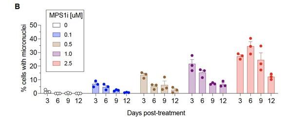
This helps support our decision to pre-treat cells with MPS1i to stimulate genomic instability and is described in the first section of Results:
“…we saw >10-fold increases of micronuclei over the cell line’s low basal level (~1% of cells), and two other MPS1i inhibitors AZ3146 and BAY12-17389 confirm such effects (Fig. S1A). Micronuclei-positive cells can persist up to 12 days after treatment (Fig. S1B), while control cells maintain the low basal levels. The results suggest pre-treatment with MPS1i can simulate CIN in an experimental context even for 1-2 weeks, which may not typically occur at the same frequency during early tumor growth.
It is known that PD-1 expression inhibits tumor-associated macrophage phagocytosis (Nature, 2017). Does MSP1i (sic) treatment affect the population of PD-1+ tumor macrophages in vivo?
We thank the Reviewer for bringing up an interesting point.
Using the same tumor RNA-seq data that was used for Fig.1E, a heatmap of expression of PD-1 (gene Pdcd1) shows no consistent trend with MPS1i:
Author response image 2.
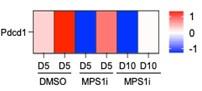
We also examined whether the secretome from CIN-afflicted cancer cells affect PD-1 expression in cultured macrophages, but we did not register any reads from our single-cell RNA-sequencing experiment for Pdcd1 in any of the macrophage clusters from Fig. 1H.
Author response image 3.
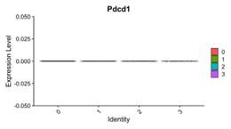
The Discussion section now includes a statement on this topic:
“…B16F10 tumors are poorly immunogenic, do not respond to either anti-CD47 or anti-PD-1/PDL1 monotherapies, and show modest and variable cure rates (~20-40%; Dooling et al., 2023; Hayes et al., 2023) even when macrophages have been made maximally phagocytic according to notions above. We should note here that our whole-tumor RNA-seq data (Fig.1E) shows expression of PD-1 (gene Pdcd1) follows no consistent trend upon MPS1i treatment, and that Pdcd1 was not detected in our scRNA-seq data for macrophage cultures (Fig.1G) – motivating further study.”
The authors must explain how the proposed therapy works since MPS1i increases tumor (cell) size, making it difficult for macrophages to phagocytose the tumor cells. It also reduces or suppresses Tyrp1 expression on the cancer cells, making it harder to opsonize. Since these were two main points for the rationale of this study, the authors need to reconcile them.
We appreciate this comment and have re-organized this Results section to try to minimize confusion:
CIN-afflicted, CD47-knockout tumoroids are eliminated by Macrophages
To assess functional effects of macrophage polarization, we focused on a 3D “immuno-tumoroid” model in which macrophage activity can work (or not) over many days against a solid proliferating mass of cancer cells in non-adherent roundbottom wells (Fig. 2A) (Dooling et al., 2023). We used CD47 knockout (KO) B16F10 cells, which removes the inhibitory effect of CD47 on phagocytosis, noting that KO does not perturb surface levels of Tyrp1, which is targetable for opsonization with anti-Tyrp1 (Fig. S2A). BMDMs were added to pre-assembled tumoroids at a 3:1 ratio, and we first assessed surface protein expression of macrophage polarization markers. Consistent with our whole-tumor bulk RNA-sequencing and also single-cell RNA-sequencing of BMDM monocultures (Fig. 1E, 1I-J), BMDMs from immunotumoroids of MPS1i-treated B16F10 showed increased surface expression of M1-like markers MHCII and CD86 while showing decreased expression of M2-like markers CD163 and CD206 (Fig. 2B-C). Although these macrophages seemed poised for anticancer activity, the cancer cells showed decreased binding of anti-Tyrp1 (Fig. S2B) and ~20% larger size in flow cytometry (Fig. S2C). The latter likely reflects cytokinesis defects and poly-ploidy as acute effects of CIN induction (Chunduri & Storchová, 2019; Mallin et al., 2022). Such cancer cell changes might explain why standard 2D phagocytosis assays show BMDMs attached to rigid plastic engulf relatively few anti-Tyrp1 opsonized cancer cells pretreated with MPS1i versus DMSO (Fig. S2D). In such cultures, BMDMs use their cytoskeleton to attach and spread, competing with engulfment of large and poorly opsonized targets. Noting that tumors in vivo are not as rigid as plastic, our 3D immunotumoroids eliminate attachment to plastic, and large numbers of macrophages can cluster and cooperate in engulfing cancer cells in a cohesive mass (Dooling et al., 2023). We indeed find CIN-afflicted tumoroids are eliminated by BMDMs regardless of anti-Tyrp1 opsonization (Fig. 2D-E), whereas anti-Tyrp1 is required for clearance of DMSO control tumoroids (Fig. 2D, S3B). Imaging also suggests that cancer CIN stimulates macrophages to cluster (compare Day-4 in Fig. 2D), which favors cooperative phagocytosis of tumoroids (Dooling et al., 2023), and occurs despite the lack of cancer cell opsonization and their larger cell size. The 3D immunotumoroid results with induced CIN are thus consistent with a more pro-phagocytic M1-type polarization (Fig.1J and 2B,C).
The authors used varying numbers of tumor cells for the in vivo portions of the study; the first half of the manuscript uses 500,000 cells, while the latter half uses 200,000 cells. Why?
The reasons for the difference in numbers is now clarified in the Methods:
For assessing immune infiltrates in early stages of tumor engraftment, when tumors are still small, we used a relatively high number of tumor cells (500,000 cells in Fig. 1D and Fig. 2F-G) to achieve sufficient cell numbers after dissociating the tumors, particularly for the slow-growing MPS1i-treated tumors. More specifically, with dissection, collagenase treatment, passage through a filter to remove clumps, we would lose many cells, and yet needed 100,000 viable cells or more for bulk RNA-seq suspensions and for flow cytometry measurements. For all other studies, 200,000 cancer cells were injected,
The authors need to report the tumor volumes and the total number of cells isolated from the day five tumors to avoid grossly inflating the effect (i.e. Fig 2G and 4G).
We have added relevant numbers in the Methods:
For day 5 post-challenge measurements, 100,000 to 200,000 live cells were collected. For in vivo tumor infiltrate studies in re-challenged mice, 10 million live cells were collected.
Also, regarding tumor sizes and cell numbers, we have previously published relevant measurements in assessments of tumor growth. Please see:
Brandon H Hayes, Hui Zhu, Jason C Andrechak, Lawrence J Dooling, Dennis E Discher, Titrating CD47 by mismatch CRISPR-interference reveals incomplete repression can eliminate IgG-opsonized tumors but limits induction of antitumor IgG, PNAS Nexus, Volume 2, Issue 8, August 2023, pgad243, https://doi.org/10.1093/pnasnexus/pgad243
Dooling, L.J., Andrechak, J.C., Hayes, B.H. et al. Cooperative phagocytosis of solid tumours by macrophages triggers durable anti-tumour responses. Nat. Biomed. Eng 7, 1081–1096 (2023). https://doi.org/10.1038/s41551-023-01031-3
In the present study, similar tumor growth curves are provided for transparency, but the Kaplan-Meier curves as the key pieces of data in Fig. 3-4. Lastly, regarding reporting total cell number harvested, we based our experiments on previously accepted measurements that also reported numbers out of total harvested cells. See:
Cerezo-Wallis, D., Contreras-Alcalde, M., … Soengas, M.S., 2020. Midkine rewires the melanoma microenvironment toward a tolerogenic and immune-resistant state. Nat Med 26, 1865–1877. https://doi.org/10.1038/s41591-020-1073-3
The figure titles need to be revised. For example, the title of Figure 1 claims that "MPS1i-induced chromosomal instability causes proliferation deficits in B16F10 tumors." However, the evidence provided is weak. The authors only present GSEA analysis of proliferation and no functional evidence of impairment. The authors need to characterize this proliferation deficit using in vitro studies and functional studies of macrophage polarization. I would suggest proliferation assays (crystal violet, MTT, Incucyte, etc) to measure the B16 growth over time with MPS1i treatment.
We thank the Reviewer for pointing this out. In Fig.1 we have minimized information regarding proliferation because it is later quantified in Figs.2D,E, S3, and 3D-i:
Fig.1F legend: Top downregulated hallmark gene sets in tumors comprised of MPS1i-treated B16F10 cells, showing downregulated DNA repair, cell cycle, and growth-related pathways, consistent with observations of slowed growth in culture and in vivo – as subsequently quantified.
Then the authors could collect the tumor supernatant to culture with macrophages and determine polarization in vitro. I would also like to see functional studies of macrophage polarization (suppression assays, cytokine production, etc). Currently, the authors provide no functional studies.
Fig.2B,C provides functional surface marker measurements of in vitro polarization toward anti-cancer M1 macrophages by MPS1i-pretreated tumor cells, consistent with gene expression in Fig.1G-J. Function is further shown as ant-cancer activity in Fig.2D,E, as now stated explicitly in the text:
“…In our 3D tumoroid in vitro assays, we found that macrophages can suppress the growth of chromosomally unstable tumoroids and clear them, surprisingly both with and without anti-Tyrp1 (Fig. 2D-E), regardless of MPS1i concentration used for treatment. Such a result is consistent with M1-type polarization (Fig.1J and 2B,C), which tends to be more pro-phagocytic. Such a result is consistent with M1-type polarization (Fig.1J and 2B,C), which tends to be more prophagocytic.”
The authors claim that macrophages are the key effector cells, but they need to provide evidence for this claim.
Other immune cells clearly contribute to the presented results because the IgG must eventually come from B cells. The text has been edited to indicate 'macrophages are key initiating-effector cells', and some evidence for this is the maximal survival of (WT B16 + Rev tumors) in Fig.3E upon treatment with Marrow Macrophages plus Macrophage-relevant SIRPa blockade and Macrophage-relevant IgG (via FcR). T cells do not have SIRPa or FcR.
They can deplete macrophages and T and B cells to determine whether the effect remains or is ablated. This is the only definitive way to make this claim.
To determine whether T and B cells might also be key initiating-effector cells, new experiments were done with mice depleted of T and B cells (per Fig.S9, below). We compared the growth of MPS1i vs DMSO treatments in these mice to results in mice with T and B cells (which should replicate our previous results in Fig.3D-i). We found that slower growth with Rev relative to DMSO was similar in mice without T and B cells compared to mice with T and B cells. We have added to the text our conclusion that: T and B cells are not key initiating-effector cells. Whereas B cells are effector cells at least in terms of eventually making anti-tumor IgG, our results show that macrophages are key initiating-effector cells because macrophages certainly affect the growth of (WT B16 + Rev tumors) when more are added (Fig.3E).
Author response image 4.
Growth of CIN-afflicted wild-type (WT) tumors in T- and B-cell deficient mice and T- and B-cell replete mice. Similar growth delays for MPS1i-pretreated B16F10 cells in T- and B-cell deficient NSG mice and immunocompetent C57BL/6 mice. Both types of mice have functional macrophages. Parallel studies in vivo were done with WT B16F10 ctrl cells cultured 24 h in 2.5 μM MPS1i (reversine or DMSO, then washed 3x in growth media for 5 min each and allowed to recover in growth media for 48 h. 200,000 cells in 100 uL PBS were injected subcutaneously into right flanks, and the standard size limit was used to determine survival curves. The C57BL/6 experiments were done independently here (by co-author L.J.D.) from the similar results (by B.H.H.) shown in Fig.3D-i, which provides evidence of reproducibility.
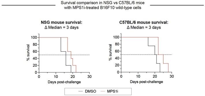
The Results section final paragraph describes all of this:
Macrophages seem to be the key initiating-effector cells, based in part on the following findings. First, macrophages with both SIRPα blockade and FcR-engaging, tumor-targeting IgG maximize survival of mice with WT B16 + Rev tumors (Fig. 3E) – noting that macrophages but not T cells express SIRPα and FcR’s. Despite the clear benefits of adding macrophages, to further assess whether T and B cells are key initiating-effector cells, new experiments were done with mice depleted of T and B cells. We compared the growth delay of MPS1i versus DMSO treatments in these mice to the delay in fully immunocompetent mice with T and B cells – with all studies done at the same time. We found that slower growth with Rev relative to DMSO was similar in mice without T and B cells when compared to immunocompetent C57 mice (Fig.S9). We conclude therefore that T and B cells are not key initiating-effector cells. At later times, B cells are likely effector cells at least in terms of making anti-tumor IgG, and T cells in tumor re-challenges are also increased in number (Fig. 4G-ii). We further note that in our earlier collaborative study (Harding et al., 2017) WT B16 cells were pre-treated by genome-damaging irradiation before engraftment in C57 mice, and these cells grew minimally – similar to MPS1i treatment – while untreated WT B16 cells grew normally at a contralateral site in the same mouse. Such results indicate that T and B cells in C57BL/6 mice are not sufficiently stimulated by genome-damaged B16 cells to generically impact the growth of undamaged B16 cells.
Reviewer #2 (Public Review):
Harnessing macrophages to attack cancer is an immunotherapy strategy that has been steadily gaining interest. Whether macrophages alone can be powerful enough to permanently eliminate a tumor is a high-priority question. In addition, the factors making different tumors more vulnerable to macrophage attack have not been completely defined. In this paper, the authors find that chromosomal instability (CIN) in cancer cells improves the effect of macrophage targeted immunotherapies. They demonstrate that CIN tumors secrete factors that polarize macrophages to a more tumoricidal fate through several methods. The most compelling experiment is transferring conditioned media from MSP1 inhibited and control cancer cells, then using RNAseq to demonstrate that the MSP1-inhibited conditioned media causes a shift towards a more tumoricidal macrophage phenotype. In mice with MSP1 inhibited (CIN) B16 melanoma tumors, a combination of CD47 knockdown and anti-Tyrp1 IgG is sufficient for long term survival in nearly all mice. This combination is a striking improvement from conditions without CIN.
Like any interesting paper, this study leaves several unanswered questions. First, how do CIN tumors repolarize macrophages? The authors demonstrate that conditioned media is sufficient for this repolarization, implicating secreted factors, but the specific mechanism is unclear. In addition, the connection between the broad, vaccination-like IgG response and CIN is not completely delineated. The authors demonstrate that mice who successfully clear CIN tumors have a broad anti-tumor IgG response. This broad IgG response has previously been demonstrated for tumors that do not have CIN. It is not clear if CIN specifically enhances the anti-tumor IgG response or if the broad IgG response is similar to other tumors. Finally, CIN is always induced with MSP1 inhibition. To specifically attribute this phenotype to CIN it would be most compelling to demonstrate that tumors with CIN unrelated to MSP1 inhibition are also able to repolarize macrophages.
Overall, this is a thought-provoking study that will be of broad interest to many different fields including cancer biology, immunology and cell biology.
We thank the Reviewer for their enthusiastic and positive comments toward the manuscript.
Our main purpose with this study has been discovery science oriented and mechanistic, with implications for improving macrophage immunotherapies. More experimentation needs to be done to further understand how this positive immune response emerges. However, we could address whether CIN enhances or not the anti-tumor IgG response by quantitative comparisons to our two other recent studies, and we conclude that it does not per new edits in the Abstract and the Results. See attached PPT for full details and comparison.
Abstract:
“CIN does not greatly affect the level of the induced response but does significantly increase survival.”
“…these results demonstrate induction of a generally potent anti-cancer antibody response to CIN-afflicted B16F10 in a CD47 KO context. Importantly, comparing these sera results for CINafflicted tumors to our recent studies of the same tumor model without CIN (Dooling et al., 2022; Hayes et al., 2022), we find similar levels of IgG induction (e.g. ~100-fold above naive on average for IgG2a/c), similar increases in phagocytosis by sera opsonization (e.g. equivalent to antiTyrp1), and similar levels of suppressed tumoroid growth – including the variability.
…
However, median survival increased (21 days) compared to their naïve counterparts (14 days), supporting the initial hypothesis of prolonged survival and consistent not only with past results indicating major benefits of a prime-&-boost approach with anti-Tyrp1 (Dooling et al., 2022) but also with the noted similarities in induced IgG levels.”
Future studies could certainly focus on trying to identify what secreted factors might be inducing the M1-like polarization (using ELISA assays for cytokine detection, for example). This could be important because a main finding here is that we achieve nearly a 100% success rate in clearing tumors when we combine CD47 ablation and IgG opsonization with cancer cell CIN. Previous studies were only able to achieve about 40% cures in mice when working with CD47 disription and IgG opsonization alone, suggesting CIN in this experimental context does improve macrophage response.
Lastly, we agree with the Reviewer that future studies should also address how CIN in general (not MPS1i-induced) affects tumor growth. The final paragraph of our Discussion at least cites support for consistent effects of M1-like polarization:
“The effects of CIN and aneuploidy in macrophages certainly requires further investigation. We did publish recently that M1-like polarization of BMDMs with IFNg priming is sufficient to suppress growth of B16 tumoroids with anti-Tyrp1 opsonization more rapidly than unpolarized/unprimed macrophages and much more rapidly than M2-like polarization of BMDMs with IL4 (Extended Data Fig.5a in Dooling et al., 2023); hence, anti-cancer polarization contributes in this assay.
While the secretome from MPS1i-treated cancer cells has been found to trigger…”
Nonetheless, we can only speculate that there is a threshold of CIN reached by a certain timepoint in tumor engraftment and growth. Natural CIN might not be enough, so we pursued a pharmacological approach consistent with ongoing pre-clinical studies (https://doi.org/10.1158/1535-7163.MCT-15-0500). Future studies should consider trying knockdown models to gradually accrue CIN in tumors or using more relevant pharmacological drugs that are known to induce CIN not associated with the spindle. We believe, however, that these are larger questions on their own and are beyond the scope of the foundational discoveries in this manuscript.
Reviewer #2 (Recommendations For The Authors):
None
We again thank the Reviewer for their support and enthusiasm for the manuscript. We made some additional changes and more data to address questions posed by the other Reviewer that we hope you find to help the manuscript further.
-
-
www.biorxiv.org www.biorxiv.org
-
Author response:
The following is the authors’ response to the original reviews.
Public Reviews:
Reviewer #1 (Public Review):
Summary:
Building upon their famous tool for the deconvolution of human transcriptomics data (EPIC), Gabriel et al. implemented a new methodology for the quantification of the cellular composition of samples profiled with Assay for Transposase-Accessible Chromatin sequencing (ATAC-Seq). To build a signature for ATAC-seq deconvolution, they first created a compendium of ATAC-seq data and derived chromatin accessibility marker peaks and reference profiles for 21 cell types, encompassing immune cells, endothelial cells, and fibroblasts. They then coupled this novel signature with the EPIC deconvolution framework based on constrained least-square regression to derive a dedicated tool called EPIC-ATAC. The method was then assessed using real and pseudo-bulk RNA-seq data from human peripheral blood mononuclear cells (PBMC) and, finally, applied to ATAC-seq data from breast cancer tumors to show it accurately quantifies their immune contexture.
Strengths:
Overall, the work is of very high quality. The proposed tool is timely; its implementation, characterization, and validation are based on rigorous methodologies and resulted in robust results. The newly-generated, validation data and the code are publicly available and well-documented. Therefore, I believe this work and the associated resources will greatly benefit the scientific community.
Weaknesses:
CA few aspects can be improved to clarify the value and applicability of the EPIC-ATAC and the transparency of the benchmarking analysis.
(1) Most of the validation results in the main text assess the methods on all cell types together, by showing the correlation, RMSE, and scatterplots of the estimated vs. true cell fractions. This approach is valuable for showing the overall method performance and for detecting systematic biases and noisy estimates. However, it provides very limited insights regarding the capability of the methods to estimate the individual cell types, which is the ultimate aim of deconvolution analysis. This limitation is exacerbated for rare cell types, which could even have a negative correlation with the ground truth fractions, but not weigh much on the overall RMSE and correlation. I would suggest integrating into the main text and figures an in-depth assessment of the individual cell types. In particular, it should be shown and discussed which cell types can be accurately quantified and which ones are less reliable.
We thank the reviewer for raising this important point. Discussing the accuracy of EPIC-ATAC in predicting individual cell-type proportions would indeed be valuable in the main text. We have updated the text as follows.
In the first version of our manuscript, we had a section called “T cell subtypes quantification reveals the ATAC-Seq deconvolution limits for closely related cell types” which highlighted that EPIC-ATAC shows low performances when predicting the proportions of cell types that are closely related, e.g., CD4+ T cell or CD8+ T cell subtypes. The section is now named “Accuracy of ATAC-Seq deconvolution is determined by the abundance and specificity of each cell type” and has been expanded to discuss the accuracy of EPIC-ATAC predictions within each major cell type.
To do so, we represented in Figure 5A the performances of EPIC-ATAC in each cell type present in the benchmarking datasets from Figures 3 and 4. Additionally, we have kept in the supplementary figures the details of the correlation values and RMSE values within each cell type and for each tool (Supplementary Figures 9 and 10). The following text has been added in the main text to describe these analyses:
“Accuracy of ATAC-Seq deconvolution is determined by the abundance and specificity of each cell type
To investigate the impact of cell type abundance on the accuracy of ATAC-Seq deconvolution, we evaluated EPIC-ATAC predictions in each major cell type separately in the different benchmarking datasets (Figure 5A). NK cells, endothelial cells, neutrophils or dendritic cells showed lower correlation values. These values can be explained by the fact that these cell types are low-abundant in our benchmarking datasets (Figure 5A). For the endothelial cells and dendritic cells, the RMSE values associated to these cell types remain low. This suggests that while the predictions of EPIC-ATAC might not be precise enough to compare these cell-type proportions between different samples, the cell-type quantification within each sample is reliable. For the NK cells and the neutrophils, we observed more variability with higher RMSE values in some datasets which suggests that the markers and profiles for these cell types might be improved. Supplementary Figures 9 and 10 detail the performances of each tool when considering each cell type separately in the PBMC and the cancer datasets. As for EPIC-ATAC, the predictions from the other deconvolution tools are more reliable for the frequent cell types.”
(2) In the benchmarking analysis, EPIC-ATAC is compared to several deconvolution methods, most of which were originally developed for transcriptomics data. This comparison is not completely fair unless their peculiarities and the limitations of tweaking them to work with ATAC-seq data are discussed. For instance, some methods (including the original EPIC) correct for cell-type-specific mRNA bias, which is not present in ATAC-seq data and might, thus, result in systematic errors.
We thank the reviewer for this comment and have updated the results and methods sections as follows:
We provide in the Materials and methods section, the paragraph “Benchmarking of the EPIC-ATAC framework against other existing deconvolution tools” which describes how each tool included in the benchmark was used in the ATAC-Seq context. We have added a reference to this section in the main text when introducing the first benchmarking analysis.
For each tool, the main changes consisted in: (i) replacing the initial RNA-Seq profiles and markers by the EPIC-ATAC reference profiles and markers and (ii) providing as input a bulk ATAC-Seq dataset with matched ATAC-Seq features (the same approach as the one used in EPIC-ATAC was considered, see answer to the next comment). Having reference profiles/markers and an ATAC-Seq bulk query with matched features was the only requirement of the different deconvolution models to be able to run on ATAC-Seq data with the default methods parameters, except for quanTIseq. Indeed, this method, like EPIC, corrects its estimations for cell-type-specific mRNA content bias. We have disabled this option for the bulk ATAC-Seq deconvolution.
We can however not exclude that a hyper parametrization of each tool could have helped to improve their current performances. Also, for RNA-Seq data deconvolution, some of the methods followed specific features filtering, e.g., the quanTIseq framework removes a manually curated list of noisy genes as well as aberrant immune genes identified in the TCGA data and ABIS uses immune-specific housekeeping genes. We can hypothesize that additional filtering could be explored for the ATAC-Seq deconvolution to improve the performance of the tools.
We have clarified these points in the results section when introducing the benchmarking, in the methods and in the discussion section.
(3) On a similar note, it could be made more explicit which adaptations were introduced in EPIC, besides the ad-hoc ATAC-seq signature, to make it applicable to this type of data.
In the first version of the manuscript, we described the changes brought to EPIC to perform bulk ATAC-Seq deconvolution in the Material and methods section in the paragraph “Running EPIC-ATAC on bulk ATAC-Seq data”. We have moved and completed this paragraph in the results section before the description of the evaluation of EPIC-ATAC in different datasets. The paragraph is the following:
“EPIC-ATAC integrates the marker peaks and profiles into EPIC to perform bulk ATAC-Seq data deconvolution
The cell-type specific marker peaks and profiles derived from the reference samples were integrated into the EPIC deconvolution tool (Racle et al., 2017; Racle and Gfeller, 2020). We will refer to this ATAC-Seq deconvolution framework as EPIC-ATAC. To ensure the compatibility of any input bulk ATAC-Seq dataset with the EPIC-ATAC marker peaks and reference profiles, we provide an option to lift over hg19 datasets to hg38 (using the liftOver R package) as the reference profiles are based on the hg38 reference genome. Subsequently, the features of the input bulk matrix are matched to our reference profiles’ features. To match both sets of features, we determine for each peak of the input bulk matrix the distance to the nearest peak in the reference profiles peaks. Overlapping regions are retained and the feature IDs are matched to their associated nearest peaks. If multiple features are matched to the same reference peak, the counts are summed. Before the estimation of the cell-type proportions, we transform the data following an approach similar to the transcripts per million (TPM) transformation which has been shown to be appropriate to estimate cell fractions from bulk mixtures in RNA-Seq data (Racle et al., 2017; Sturm et al., 2019). We normalize the ATAC-Seq counts by dividing counts by the peak lengths as well as samples depth and rescaling counts so that the counts of each sample sum to 106. In RNA-Seq based deconvolution, EPIC uses an estimation of the amount of mRNA in each reference cell type to derive cell proportions while correcting for cell-type-specific mRNA bias. For the ATAC-Seq based deconvolution these values were set to 1 to give similar weights to all cell-types quantifications. Indeed ATAC-Seq measures signal at the DNA level, hence the quantity of DNA within each reference cell type is similar.”
(4) Given that the final applicability of EPIC-ATAC is on real bulk RNA-seq data, whose characteristics might not be completely recapitulated by pseudo-bulk samples, it would be interesting to see EPIC and EPIC-ATAC compared on a dataset with matched, real bulk RNA-seq and ATAC-seq, respectively. It would nicely complement the analysis of Figure 7 and could be used to dissect the commonalities and peculiarities of these two approaches.
We thank the reviewer for raising this important point. EPIC-ATAC will be applied to real bulk ATAC-Seq data and pseudobulk data cannot indeed fully recapitulate the bulk signals. Recently, a dataset composed of more than 100 samples with matched bulk RNA-Seq, bulk ATAC-Seq as well as matched flow cytometry data has been published by Morandini and colleagues in GeroScience in November 2023. We thus retrieved these data to compare the predictions obtained by EPIC-ATAC on the bulk ATAC-Seq data and the predictions of the original version of EPIC on the bulk RNA-Seq data to the cell-type quantification obtained by flow cytometry. We also assessed whether both modalities could be complementary using a simple approach averaging the predictions obtained from both modalities. The results of these analyzes have been summarized in the Figure 7C and are described in the main text in the last paragraph of the paper:
“We compared the predictions obtained using each modality to the flow cytometry cell-type quantifications. EPIC-ATAC predictions were better correlated with the flow cytometry measures for some cell types (e.g., CD8+, CD4+ T cells, NK cells) while this trend was observed with the EPIC-RNA predictions in other cell types (B cells, neutrophils, monocytes) (Figure 7C). We then tested whether the predictions obtained from both modalities could be combined to improve the accuracy of each cell-type quantification. Averaging the predictions obtained from both modalities shows a moderate improvement (Figure 7C), suggesting that the two modalities can complement each other.”
Reviewer #2 (Public Review):
Summary:
The manuscript expands the current bulk sequencing data deconvolution toolkit to include ATAC-seq. The EPIC-ATAC tool successfully predicts accurate proportions of immune cells in bulk tumour samples and EPIC-ATAC seems to perform well in benchmarking analyses. The authors achieve their aim of developing a new bulk ATAC-seq deconvolution tool.
Strengths:
The manuscript describes simple and understandable experiments to demonstrate the accuracy of EPIC-ATAC. They have also been incredibly thorough with their reference dataset collections. The authors have been robust in their benchmarking endeavours and measured EPIC-ATAC against multiple datasets and tools.
Weaknesses:
Currently, the tool has a narrow applicability in that it estimates the percentage of immune cells in a bulk ATAC-seq experiment.
Comments:
(1) Has any benchmarking been done on the runtime of the tool? Although EPIC-ATAC seems to "win" in benchmarking metrics, sometimes the differences are quite small. If EPIC-ATAC takes forever to run, compared to another tool that is a lot quicker, might some people prefer to sacrifice 0.01 in correlation for a quicker running tool?
We thank the reviewer for raising this point that was not addressed in the manuscript. We have added a supplementary figure (Supplementary Figure 8) which represents the CPU time used by each tool. The figure shows that all the tools could be run in less than 20 seconds in average. This figure has been mentioned at the end of the benchmarking paragraphs.
(2) In Figure 3B the data points look a bit squashed in the bottom-left corner. Could the plot be replotted with the data point spread out? There also seems to be some inter-patient variability. Could the authors comment on that?
We have updated Figure 3B to increase the visibility of the dots in the bottom-left corner. To do so, we have limited the x and y axes to the maximum of the predicted proportions for the y axis and true proportions for the x axis.
We also acknowledge that the accuracy of the predictions varies across samples. In particular, one sample (Sample4, star shape on Figure 3B) exhibits larger discrepancies between EPIC-ATAC predictions and the ground truth. To understand the lower performance, we have visualized our marker peaks in the five PBMC samples (Figure below). Based on this visualization, we can see that Sample4 might be an outlier sample considering that its cellular composition is similar to that of Sample2 and Sample5, however this sample shows particularly high ATAC-Seq accessibility at the monocytes and dendritic markers. This can explain why EPIC-ATAC overestimates the proportions of the two populations in this case. We have added the previously mentioned figures as a Supplementary Figure (Supplementary Figure 2) and have described it in the results section in the paragraph “EPIC-ATAC accurately estimates immune cell fractions in PBMC ATAC-Seq samples”.
(3) Could the authors comment on the possibility of expanding EPIC-ATAC into more than a percentage prediction tool? Perhaps EPIC-ATAC could remove the immune cell signal from the bulk ATAC-seq data to "purify" the uncharacterised cells in silico, or generate pseudo-ATAC-seq tracks of the identified cell types.
We thank the reviewer for this interesting question. As suggested by the reviewer, one approach to purify bulk genomics data using the cell-type proportions estimated by a cell-type deconvolution tool is to subtract the weighted sum of the signal observed in the reference data, weights corresponding to the predicted proportions. We used this approach on the EPIC-ATAC predictions obtained from pseudobulks built from scATAC-Seq data from diverse cancer types coming from the Human Tumor Atlas Network (HTAN) (See also the answer of the first recommendation of Reviewer 1). This dataset allows us to compare for a relatively large number of samples (a maximum of 25 samples in a cancer type cohort) the purified signal to the true signal derived from the single-cell data. The results are presented in the figure below which shows that the correlations between the predicted and true signals are relatively good in most of the cancer types (blue boxplots). However, these correlation levels are lower than the ones obtained when comparing the signal obtained from the entire pseudobulk (red boxplots) with the true signal. This suggests that this purification approach leads to a signal that is less precise and accurate than the signal resulting from all cells mixtures.
Author response image 1.
Boxplots of the correlation values obtained from the comparison of the bulk signal and the ground truth signal from the uncharacterized cells in each sample (red) and from the comparison of the predicted signal and the ground truth signal from the uncharacterized cells in each sample (blue).
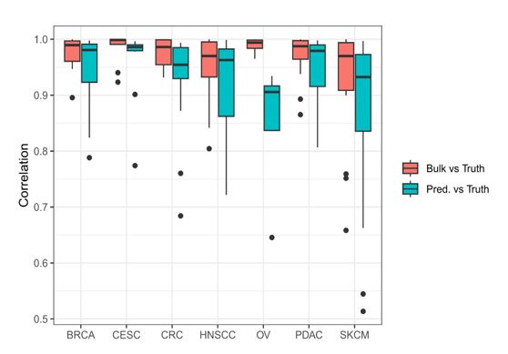
Also, note that in our simple approach, negative values can be obtained. The predicted signal will thus be difficult to interpret and to use in downstream analyses. Methods claiming to perform purification of bulk samples use more complex and dedicated algorithms. For example, Symphony (Burdziak et al., 2019) (cited in our introduction) uses single-cell RNA-Seq data in addition to the bulk chromatin accessibility data to infer cluster-specific accessibility profiles. Considering that EPIC was not designed for purification purposes, we decided not to include this analysis in the updated version of the manuscript.
Recommendations For The Authors:
Reviewer #1 (Recommendations For The Authors):
(1) The original EPIC had two different signatures for application to blood or tumor RNA-seq. It is not clear instead if EPIC-ATAC applies with the same signature and framework to any tissue and disease context. This aspect should be clarified in the text.
We thank the reviewer for raising this point which was not clear in the previous version of the manuscript. As in the original version of EPIC, in EPIC-ATAC two reference profiles and sets of markers are available, the PBMC reference and the TME reference. We used the PBMC reference profiles and markers to deconvolve the PBMC samples and the TME reference profiles and markers to deconvolve the cancer samples. We have clarified this point in the result section of the main text in the paragraph “ATAC-Seq data from sorted cell populations reveal cell-type specific marker peaks and reference profiles” as follows (added text underlined):
“The resulting marker peaks specific only to the immune cell types were considered for the deconvolution of PBMC samples (PBMC markers). For the deconvolution of tumor bulk samples, the lists of marker peaks specific to fibroblasts and endothelial cells were added to the PBMC markers. This extended set of markers was further refined based on the correlation patterns of the markers in tumor bulk samples from the diverse solid cancer types from The Cancer Genome Atlas (TCGA) (Corces et al., 2018), i.e., markers exhibiting the highest correlation patterns in the tumor bulk samples were selected using the findCorrelation function from the caret R package (Kuhn, 2008) (Figure 1, box 4, see the Material and methods, section 2). The latter filtering ensures the relevance of the markers in the TME context since cell-type specific TME markers are expected to be correlated in tumor bulk ATAC-Seq measurements (Qiu et al., 2021). 716 markers of immune, fibroblasts and endothelial cell types remained after the last filtering (defined as TME markers). Considering the difference in cell types and the different filtering steps applied on the PBMC and TME markers, we recommend to use the TME markers and profiles to deconvolve bulk samples from tumor samples and the PBMC markers and profiles to deconvolve PBMC samples.”
We also note that when running EPIC-ATAC using the PBMC markers and the TME markers independently to perform the deconvolution of the cancer datasets, we see that overall the use of the TME markers leads to a better performance (Figure below).
Figure legend: Correlation and RMSE values obtained when running EPIC-ATAC on each cancer dataset (points) using the PBMC (red) and the TME (blue) markers.
To demonstrate that the TME markers can be applied to different cancer types, we have completed the evaluation of EPIC-ATAC on tumor samples by considering an additional dataset: the Human Tumor Atlas Network (HTAN) single-cell multiomic (scRNA-Seq and scATAC-Seq) dataset. We have processed this dataset and built scATAC-Seq pseudobulks for 7 cancer types on which EPIC-ATAC was applied to. This analysis has been summarized in Figure 4 and Supplementary Figure 4 and shows that EPIC-ATAC is applicable in a diverse set of tissues.
(2) EPIC and EPIC-ATAC have a valuable feature, which is absent from most deconvolution methods: the estimation of unknown content. It would be informative for the users to understand from the benchmarking analysis whether this feature gives an advantage to EPIC-ATAC with respect to the other approaches.
Indeed, among the tools that we included in our benchmarking analysis, only EPIC-ATAC and quanTIseq enable users to predict the proportions of cells that are not present in the reference profiles, i.e., the uncharacterized cells. For the other tools we thus fixed the estimated proportions of uncharacterized cells to 0. This approach provides a clear and significant advantage to EPIC-ATAC and to quanTIseq. For this reason, we also provide a version of the benchmarking in which we exclude the uncharacterized cells and rescale the true and estimated cell-type proportions to sum to 1. In this second benchmarking approach, EPIC-ATAC still outperforms some of the other deconvolution tools.
We have clarified this point in the results section, in the paragraph “EPIC-ATAC accurately predicts fractions of cancer and non-malignant cells in tumor samples”.
(3) The selection of the most discriminative markers is very well described in the text and beautifully illustrated in Figure 2. However, it is unclear why UMAP plots are used to represent cell-type similarities and dissimilarities. Would a linear dimensionality reduction approach like PCA be already sufficient to show these groups, especially considering the not-so-extreme dimensionality of the underlying data? In addition, a statistic that could be also considered to compare clusters to the cell type labels in the two scenarios is the Adjusted Rand Index (ARI).
We thank the reviewer for this relevant comment. We initially used UMAP to facilitate the visualization of the different cell-type groups. However, it is true that the three first axes of the principal component analyses performed based on each set of marker peaks already capture most of the structure in the data and that the use of UMAP can lead to an artificial enhancement of separation between the different groups of cells. We have updated Figure 2B by replacing the UMAP scatter plots by 3D representations of the first three principal components of the PCA and have added in Supplementary Figure 1B the pairwise scatter plots of these first 3 principal components. On the main figures, we have also added the ARI metric comparing the cell-type annotation and the clustering obtained using the first 10 axes of the PCA and model based clustering.
(4) In the introduction, it is stated that "the reasonable cost and technical advantages of these protocols foreshadow an increased usage of ATAC-Seq in cancer studies". I would suggest adding a reference to justify this trend. Also, it should be discussed how ATAC-seq deconvolution compares to other types of deconvolution approaches applied to cheaper epigenetic data like methylation one (e.g. epidish, methylcc, tca, minfi).
We have complemented this sentence with two references to justify the assertion: (i) a review published by Luo, Gribskov and Wang in 2022 showing the increasing number of ATAC-Seq studies in the field of cancer research, and (ii) a protocol paper from Grandi et al. published in 2022 on the state-of-the-art Omni-ATAC protocol for ATAC-sequencing which discusses the broad applicability and the technical advantages of ATAC-sequencing. Also in the preceding sentence, a recent ATAC-Seq protocol that can be applied to FFPE samples has been mentioned, FFPE samples being the most common samples in clinical cancer research.
We agree with the reviewer on the fact that other epigenetic assays such as methylation assays are cost effective. However, ATAC-sequencing provides additional information on the epigenetic landscape of a sample’s genome and some questions regarding regulatory regions and transcription factor activity cannot be answered with methylation data. Methods that can be applied on ATAC-Seq data specifically are thus needed. Most of the cell-type deconvolution algorithms existing so far are applicable on RNA-Seq or methylation data. These algorithms often use similar methodological concepts, e.g., linear combination of the reference profiles for reference-based methods, which could be used in different modalities. However, methylation-based deconvolution tools often take as input a data format that is specific to methylation data, e.g., two color micro array data (RGChannelSet R object) for the minfi deconvolution function (estimatesCellCounts) or leverage methylation-specific information to perform the deconvolution. For example, methylCC uses a model based on latent variables representing a binarized measures of the methylation status of cell-type specific regions (1 or 0 for clearly methylated or unmethylated regions). Such methods are more difficult to adapt than tools based on RNA-Seq data where the signal is quantified using read counts similarly to ATAC-Seq data.
Nevertheless, some methods such as EPIdish or MethylCIBERSORT have proposed new methylation reference profiles and have used existing models that are not specific to methylation data to deconvolve the bulk data. In our work, we followed a similar approach where we propose new reference profiles specific to chromatin accessibility data, integrate them to an existing method EPIC as well as test them in other existing tools. Note that methylation reference profiles cannot be directly used for ATAC-Seq data deconvolution considering that methylation measures methylation status at CpG sites (dinucleotides) and ATAC-Seq measures the accessibility of regions of hundreds base pairs.
An analysis comparing the performance of methylation-based deconvolution and ATAC-Seq based deconvolution would be informative. However, such analysis is beyond the scope of our paper considering that none of the datasets used for our benchmarking provide these two modalities for the same samples.
In the manuscript, we have completed the references associated to the methylation-based deconvolution tools with the ones mentioned in the previous paragraphs and by the reviewer and have completed the discussion as follows:
“The comparison of EPIC-ATAC applied on ATAC-Seq data with EPIC applied on RNA-Seq data has shown that both modalities led to similar performances and that they could complement each other. Another modality that has been frequently used in the context of bulk sample deconvolution is methylation. Methylation profiling techniques such as methylation arrays are cost effective (Kaur et al., 2023) and DNA methylation signal is highly cell-type specific (Kaur et al., 2023; Loyfer et al., 2023). Considering that methylation and chromatin accessibility measure different features of the epigenome, additional analyses comparing and/or complementing ATAC-seq based deconvolution with methylation-based deconvolution could be of interest as future datasets profiling both modalities in the same samples become available.”
(5) In the Results section, some methodological steps could be phrased in a bit more extensive way to let the reader understand the rationale and the actual approach. I recognize there is also a reference to the Methods section, where all methodologies are reported in detail, but some of the sentences are hard to understand due to their synthetic format, e.g.: "markers with potential residual accessibility in human tissues were then filtered out".
We thank the reviewer for this comment and we have followed his recommendation to expand sentences with a synthetic format. Text changes and additions are underlined below:
“To limit batch effects, the collected samples were homogeneously processed from read alignment to peak calling. For each cell type, we derived a set of stable peaks observed across samples and studies, i.e. for each study, peaks detected in at least half of the samples were considered, and for each cell type, only peaks detected jointly in all studies were kept (see Materials and Methods, section 1).”
“To filter out markers that could be accessible in other human cell-types than those included in our reference profiles, we used the human atlas study (K. Zhang et al., 2021), which identified modules of open chromatin regions accessible in a comprehensive set of human tissues, and we excluded from our marker list the markers overlapping these modules (Figure 1, box 3, see Materials and Methods section 2).”
“For the deconvolution of tumor bulk samples, the lists of marker peaks specific to fibroblasts and endothelial cells were added to the PBMC markers. This extended set of markers was further refined based on the correlation patterns of the markers in tumor bulk samples from the diverse solid cancer types from The Cancer Genome Atlas (TCGA) (Corces et al., 2018), i.e., markers exhibiting the highest correlation patterns in the tumor bulk samples were selected using the findCorrelation function from the caret R package (Kuhn, 2008) (Figure 1, box 4, see the Material and methods, section 2).”
Also, following the comments and recommendations of the Reviewer 1, we have: (i) moved the method section describing the adaptation of EPIC to ATACseq data to provide more details in the results section (see answer to the third comment of Reviewer 1), (ii) clarified how the existing tools used in the benchmarking analyses were adapted for ATAC-Seq deconvolution (see answer to the second comment of Reviewer 1), and (iii) detailed how the comparison between our estimations of the infiltration levels in the samples from Kumegawa et al. and the estimations from the original study was performed (see answer to the seventh recommendation of Reviewer 1).
(6) In the main text, it is stated that "the list of markers was further refined based on the correlation patterns of the markers in tumor bulk samples from diverse cancer types from The Cancer Genome Atlas". It should be clarified if these are only solid cancers, or if blood cancers were also used.
We have considered only the solid cancers and have clarified this point in the results section: “This extended set of markers was further refined based on the correlation patterns of the markers in tumor bulk samples from the diverse solid cancer types from The Cancer Genome Atlas”.
(7) When reporting that "these predictions are consistent with the infiltration level estimations reported in the original publication", it should be mentioned how the infiltration levels were quantified in this publication and how this agreement was quantified. This would be important also to claim in the abstract that "EPIC-ATAC accurately infers the immune contexture of the main breast cancer subtypes".
We thank the reviewer for this comment, we acknowledge that the agreement between the EPIC-ATAC predictions and the infiltration levels quantified in the original publication should be further described in the paper. We have expanded the text in the results section in the paragraph “EPIC-ATAC accurately infers the immune contexture in a bulk ATAC-Seq breast cancer cohort” to clarify this point. Additionally, we have added a panel in Figure 6 (panel A) which shows a good agreement between EPIC-ATAC predictions and the metric used in the original paper to evaluate the infiltration levels of different cell types.
The added text is underlined below:
“We applied EPIC-ATAC to a breast cancer cohort of 42 breast ATAC-Seq samples including samples from two breast cancer subtypes, i.e., 35 oestrogen receptor (ER)-positive human epidermal growth factor receptor 2 (HER2)-negative (ER+/HER2-) samples and 7 triple negative (TNBC) tumors (Kumegawa et al., 2023). No cell sorting was performed in parallel to the chromatin accessibility sequencing. For this reason, the authors used a set of cell-type-specific cis-regulatory elements (CREs) identified in scATAC-Seq data from similar breast cancer samples (Kumegawa et al., 2022) and estimated the amount of infiltration of each cell type by averaging the ATAC-Seq signal of each set of cell-type-specific CREs in their samples. We used EPIC-ATAC to estimate the proportions of different cell types of the TME. These predictions were then compared to the metric used by Kumegawa and colleagues in their study to infer levels of infiltration. A high correlation between the two metrics was observed for each cell type (Pearson’s correlation coefficient from 0.5 for myeloid cells to 0.94 for T cells, Figure 6A).”
(8) It should be made explicit if EPIC-ATAC quantifies mDC, pDC, or their sum.
In our collection of reference ATAC-Seq samples from which the markers and profiles have been derived, mDCs and pDCs were both included in the dendritic cells. EPIC-ATAC thus quantifies the total amount of dendritic cells, i.e., mDCs and pDCs included. We have added a sentence in the main text to clarify this point:
To identify robust chromatin accessibility marker peaks of cancer relevant cell types, we collected 564 samples of sorted cell populations from twelve studies including eight immune cell types (B cells […] dendritic cells (DCs) (mDCs and pDCs are grouped in this cell-type category) […] and endothelial (Liu et al., 2020; Xin et al., 2020) cells (Figure 1 box 1, Figure 2A, Supplementary Table 1).
Reviewer #2 (Recommendations For The Authors):
The authors should double-check the naming of tools is done correctly e.g. ChIPSeeker has been spelled incorrectly in some instances throughout the manuscript.
We thank the reviewer for pointing out this mistake and have corrected the mistake in the main text.
-
-
-
Amazon Plans to Replace More Than Half a Million Jobs With Robots
- Internal documents reviewed by The New York Times show Amazon plans to automate up to 75% of its operations in the coming years.
- The company expects automation to replace or eliminate over 500,000 U.S. jobs by 2033, primarily in warehouses and fulfillment centers.
- By 2027, automation could allow Amazon to avoid hiring around 160,000 new workers, saving about 30 cents per package shipped.
- This strategy is projected to save $12.6 billion in labor costs between 2025 and 2027.
- Amazon’s workforce tripled since 2018 to approximately 1.2 million U.S. employees, but automation is expected to stabilize or reduce future headcount despite rising sales.
- Executives presented to the board that automation could let the company double sales volume by 2033 without needing additional hires.
- Amazon’s Shreveport, Louisiana warehouse serves as the model for the future: it operates with 25% fewer workers and about 1,000 robots.
- A new facility in Virginia Beach and retrofitted older ones like Stone Mountain, Georgia, are following this design, which may shift employment toward more temporary and technical roles.
- The company is instructing staff to use softer language—such as “advanced technology” or “cobots” (collaborative robots)—instead of terms like “AI” or “robots,” to ease concerns about job loss.
- Amazon has begun planning community outreach initiatives (parades, local events) to offset the reputational risks of large-scale automation.
- The company has denied that the documents represent official policy, claiming they reflect the views of one internal group, and emphasized ongoing seasonal hiring (250,000 roles for holidays).
- Analysts suggest this plan could serve as a blueprint for other major employers, including Walmart and UPS, potentially reshaping U.S. blue‑collar job markets.
- The automation push continues a trajectory started with Amazon’s $775 million acquisition of Kiva Systems in 2012, which introduced mobile warehouse robots that revolutionized internal logistics.
- Recent innovations include robots like Blue Jay, Vulcan, and Proteus, aimed at performing tasks such as sorting, picking, and packaging with minimal human oversight.
- Long-term, Amazon may require fewer warehouse workers but more robot technicians and engineers, signaling a broader shift in labor type rather than total employment.
-
-
www.biorxiv.org www.biorxiv.org
-
Author response:
The following is the authors’ response to the original reviews
We thank all the reviewers for their constructive comments. We have carefully considered your feedback and revised the manuscript accordingly. The major concern raised was the applicability of SegPore to the RNA004 dataset. To address this, we compared SegPore with f5c and Uncalled4 on RNA004, and found that SegPore demonstrated improved performance, as shown in Table 2 of the revised manuscript.
Following the reviewers’ recommendations, we updated Figures 3 and 4. Additionally, we added one table and three supplementary figures to the revised manuscript:
· Table 2: Segmentation benchmark on RNA004 data
· Supplementary Figure S4: RNA translocation hypothesis illustrated on RNA004 data
· Supplementary Figure S5: Illustration of Nanopolish raw signal segmentation with eventalign results
· Supplementary Figure S6: Running time of SegPore on datasets of varying sizes
Below, we provide a point-by-point response to your comments.
Reviewer #1 (Public review):
Summary:
In this manuscript, the authors describe a new computational method (SegPore), which segments the raw signal from nanopore-direct RNA-Seq data to improve the identification of RNA modifications. In addition to signal segmentation, SegPore includes a Gaussian Mixture Model approach to differentiate modified and unmodified bases. SegPore uses Nanopolish to define a first segmentation, which is then refined into base and transition blocks. SegPore also includes a modification prediction model that is included in the output. The authors evaluate the segmentation in comparison to Nanopolish and Tombo, and they evaluate the impact on m6A RNA modification detection using data with known m6A sites. In comparison to existing methods, SegPore appears to improve the ability to detect m6A, suggesting that this approach could be used to improve the analysis of direct RNA-Seq data.
Strengths:
SegPore addresses an important problem (signal data segmentation). By refining the signal into transition and base blocks, noise appears to be reduced, leading to improved m6A identification at the site level as well as for single-read predictions. The authors provide a fully documented implementation, including a GPU version that reduces run time. The authors provide a detailed methods description, and the approach to refine segments appears to be new.
Weaknesses:
In addition to Nanopolish and Tombo, f5c and Uncalled4 can also be used for segmentation, however, the comparison to these methods is not shown.
The method was only applied to data from the RNA002 direct RNA-Sequencing version, which is not available anymore, currently, it remains unclear if the methods still work on RNA004.
Thank you for your comments.
To clarify the background, there are two kits for Nanopore direct RNA sequencing: RNA002 (the older version) and RNA004 (the newer version). Oxford Nanopore Technologies (ONT) introduced the RNA004 kit in early 2024 and has since discontinued RNA002. Consequently, most public datasets are based on RNA002, with relatively few available for RNA004 (as of 30 June 2025).
Nanopolish and Tombo were developed for raw signal segmentation and alignment using RNA002 data, whereas f5c and Uncalled4are the only two software supporting RNA004 data. Since the development of SegPore began in January 2022, we initially focused on RNA002 due to its data availability. Accordingly, our original comparisons were made against Nanopolish and Tombo using RNA002 data.
We have now updated SegPore to support RNA004 and compared its performance against f5c and Uncalled4 on three public RNA004 datasets.
As shown in Table 2 of the revised manuscript, SegPore outperforms both f5c and Uncalled4 in raw signal segmentation. Moreover, the jiggling translocation hypothesis underlying SegPore is further supported, as shown in Supplementary Figure S4.
The overall improvement in accuracy appears to be relatively small.
Thank you for the comment.
We understand that the improvements shown in Tables 1 and 2 may appear modest at first glance due to the small differences in the reported standard deviation (std) values. However, even small absolute changes in std can correspond to substantial relative reductions in noise, especially when the total variance is low.
To better quantify the improvement, we assume that approximately 20% of the std for Nanopolish, Tombo, f5c, and Uncalled4 arises from noise. Using this assumption, we calculate the relative noise reduction rate of SegPore as follows:
Noise reduction rate = (baseline std − SegPore std) / (0.2 × baseline std)
Based on this formula, the average noise reduction rates across all datasets are:
- SegPore vs Nanopolish: 49.52%
- SegPore vs Tombo: 167.80%
- SegPore vs f5c: 9.44%
- SegPore vs Uncalled4: 136.70%
These results demonstrate that SegPore can reduce the noise level by at least 9% given a noise level of 20%, which we consider a meaningful improvement for downstream tasks, such as base modification detection and signal interpretation. The high noise reduction rates observed in Tombo and Uncalled4 (over 100%) suggest that their actual noise proportion may be higher than our 20% assumption.
We acknowledge that this 20% noise level assumption is an approximation. Our intention is to illustrate that SegPore provides measurable improvements in relative terms, even when absolute differences appear small.
The run time and resources that are required to run SegPore are not shown, however, it appears that the GPU version is essential, which could limit the application of this method in practice.
Thank you for your comment.
Detailed instructions for running SegPore are provided in github (https://github.com/guangzhaocs/SegPore). Regarding computational resources, SegPore currently requires one CPU core and one Nvidia GPU to perform the segmentation task efficiently.
We present SegPore’s runtime for typical datasets in Supplementary Figure S6 in the revised manuscript. For a typical 1 GB fast5 file, the segmentation takes approximately 9.4 hours using a single NVIDIA DGX‑1 V100 GPU and one CPU core.
Currently, GPU acceleration is essential to achieve practical runtimes with SegPore. We acknowledge that this requirement may limit accessibility in some environments. To address this, we are actively working on a full C++ implementation of SegPore that will support CPU-only execution. While development is ongoing, we aim to release this version in a future update.
Reviewer #2 (Public review):
Summary:
The work seeks to improve the detection of RNA m6A modifications using Nanopore sequencing through improvements in raw data analysis. These improvements are said to be in the segmentation of the raw data, although the work appears to position the alignment of raw data to the reference sequence and some further processing as part of the segmentation, and result statistics are mostly shown on the 'data-assigned-to-kmer' level.
As such, the title, abstract, and introduction stating the improvement of just the 'segmentation' does not seem to match the work the manuscript actually presents, as the wording seems a bit too limited for the work involved.
The work itself shows minor improvements in m6Anet when replacing Nanopolish eventalign with this new approach, but clear improvements in the distributions of data assigned per kmer. However, these assignments were improved well enough to enable m6A calling from them directly, both at site-level and at read-level.
Strengths:
A large part of the improvements shown appear to stem from the addition of extra, non-base/kmer specific, states in the segmentation/assignment of the raw data, removing a significant portion of what can be considered technical noise for further analysis. Previous methods enforced the assignment of all raw data, forcing a technically optimal alignment that may lead to suboptimal results in downstream processing as data points could be assigned to neighbouring kmers instead, while random noise that is assigned to the correct kmer may also lead to errors in modification detection.
For an optimal alignment between the raw signal and the reference sequence, this approach may yield improvements for downstream processing using other tools.<br /> Additionally, the GMM used for calling the m6A modifications provides a useful, simple, and understandable logic to explain the reason a modification was called, as opposed to the black models that are nowadays often employed for these types of tasks.
Weaknesses:
The work seems limited in applicability largely due to the focus on the R9's 5mer models. The R9 flow cells are phased out and not available to buy anymore. Instead, the R10 flow cells with larger kmer models are the new standard, and the applicability of this tool on such data is not shown. We may expect similar behaviour from the raw sequencing data where the noise and transition states are still helpful, but the increased kmer size introduces a large amount of extra computing required to process data and without knowledge of how SegPore scales, it is difficult to tell how useful it will really be. The discussion suggests possible accuracy improvements moving to 7mers or 9mers, but no reason why this was not attempted.
Thank you for pointing out this important limitation. Please refer to our response to Point 1 of Reviewer 1 for SegPore’s performance on RNA004 data. Notably, the jiggling behavior is also observed in RNA004 data, and SegPore achieves better performance than both f5c and Uncalled4.
The increased k-mer size in RNA004 affects only the training phase of SegPore (refer to Supplementary Note 1, Figure 5 for details on the training and testing phases). Once the baseline means and standard deviations for each k-mer are established, applying SegPore to RNA004 data proceeds similarly to RNA002. This is because each k-mer in the reference sequence has, at most, two states (modified and unmodified). While the larger k-mer size increases the size of the parameter table, it does not increase the computational complexity during segmentation. Although estimating the initial k-mer parameter table requires significant time and effort on our part, it does not affect the runtime for end users applying SegPore to RNA004 data.
Extending SegPore from 5-mers to 7-mers or 9-mers for RNA002 data would require substantial effort to retrain the model and generate sufficient training data. Additionally, such an extension would make SegPore’s output incompatible with widely used upstream and downstream tools such as Nanopolish and m6Anet, complicating integration and comparison. For these reasons, we leave this extension for future work.
The manuscript suggests the eventalign results are improved compared to Nanopolish. While this is believably shown to be true (Table 1), the effect on the use case presented, downstream differentiation between modified and unmodified status on a base/kmer, is likely limited as during actual modification calling the noisy distributions are usually 'good enough', and not skewed significantly in one direction to really affect the results too terribly.
Thank you for your comment. While current state-of-the-art (SOTA) methods perform well on benchmark datasets, there remains significant room for improvement. Most SOTA evaluations are based on limited datasets, primarily covering DRACH motifs in human and mouse transcriptomes. However, m6A modifications can also occur in non-DRACH motifs, where current models may underperform. Additionally, other RNA modifications—such as pseudouridine, inosine, and m5C—are less studied, and their detection may benefit from improved signal modeling.
We would also like to emphasize that raw signal segmentation and RNA modification detection are distinct tasks. SegPore focuses on the former, providing a cleaner, more interpretable signal that can serve as a foundation for downstream tasks. Improved segmentation may facilitate the development of more accurate RNA modification detection algorithms by the community.
Scientific progress often builds incrementally through targeted improvements to foundational components. We believe that enhancing signal segmentation, as SegPore does, contributes meaningfully to the broader field—the full impact will become clearer as the tool is adopted into more complex workflows.
Furthermore, looking at alternative approaches where this kind of segmentation could be applied, Nanopolish uses the main segmentation+alignment for a first alignment and follows up with a form of targeted local realignment/HMM test for modification calling (and for training too), decreasing the need for the near-perfect segmentation+alignment this work attempts to provide. Any tool applying a similar strategy probably largely negates the problems this manuscript aims to improve upon.
We thank the reviewer for this insightful comment.
To clarify, Nanopolish provides three independent commands: polya, eventalign, and call-methylation.
- The polya command identifies the adapter, poly(A) tail, and transcript region in the raw signal.
- The eventalign command aligns the raw signal to a reference sequence, assigning a signal segment to individual k-mers in the reference.
- The call-methylation command detects methylated bases from DNA sequencing data.
The eventalign command corresponds to “the main segmentation+alignment for a first alignment,” while call-methylation corresponds to “a form of targeted local realignment/HMM test for modification calling,” as mentioned in the reviewer’s comment. SegPore’s segmentation is similar in purpose to Nanopolish’s eventalign, while its RNA modification estimation component is similar in concept to Nanopolish’s call-methylation.
We agree the general idea may appear similar, but the implementations are entirely different. Importantly, Nanopolish’s call-methylation is designed for DNA sequencing data, and its models are not trained to recognize RNA modifications. This means they address distinct research questions and cannot be directly compared on the same RNA modification estimation task. However, it is valid to compare them on the segmentation task, where SegPore exhibits better performance (Table 1).
We infer the reviewer may suggest that because m6Anet is a deep neural network capable of learning from noisy input, the benefit of more accurate segmentation (such as that provided by SegPore) might be limited. This concern may arise from the limited improvement of SegPore+m6Anet over Nanopolish+m6Anet in bulk analysis (Figure 3). Several factors may contribute to this observation:
(i) For reads aligned to the same gene in the in vivo data, alignment may be inaccurate due to pseudogenes or transcript isoforms.
(ii) The in vivo benchmark data are inherently more complex than in vitro datasets and may contain additional modifications (e.g., m5C, m7G), which can confound m6A calling by altering the signal baselines of k-mers.
(iii) m6Anet is trained on events produced by Nanopolish and may not be optimal for SegPore-derived events.
(iv) The benchmark dataset lacks a modification-free (IVT) control sample, making it difficult to establish a true baseline for each k-mer.
In the IVT data (Figure 4), SegPore shows a clear improvement in single-molecule m6A identification, with a 3~4% gain in both ROC-AUC and PR-AUC. This demonstrates SegPore’s practical benefit for applications requiring higher sensitivity at the molecule level.
As noted earlier, SegPore’s contribution lies in denoising and improving the accuracy of raw signal segmentation, which is a foundational step in many downstream analyses. While it may not yet lead to a dramatic improvement in all applications, it already provides valuable insights into the sequencing process (e.g., cleaner signal profiles in Figure 4) and enables measurable gains in modification detection at the single-read level. We believe SegPore lays the groundwork for developing more accurate and generalizable RNA modification detection tools beyond m6A.
We have also added the following sentence in the discussion to highlight SegPore’s limited performance in bulk analysis:
“The limited improvement of SegPore combined with m6Anet over Nanopolish+m6Anet in bulk in vivo analysis (Figure 3) may be explained by several factors: potential alignment inaccuracies due to pseudogenes or transcript isoforms, the complexity of in vivo datasets containing additional RNA modifications (e.g., m5C, m7G) affecting signal baselines, and the fact that m6Anet is specifically trained on events produced by Nanopolish rather than SegPore. Additionally, the lack of a modification-free control (in vitro transcribed) sample in the benchmark dataset makes it difficult to establish true baselines for each k-mer. Despite these limitations, SegPore demonstrates clear improvement in single-molecule m6A identification in IVT data (Figure 4), suggesting it is particularly well suited for in vitro transcription data analysis.”
Finally, in the segmentation/alignment comparison to Nanopolish, the latter was not fitted(/trained) on the same data but appears to use the pre-trained model it comes with. For the sake of comparing segmentation/alignment quality directly, fitting Nanopolish on the same data used for SegPore could remove the influences of using different training datasets and focus on differences stemming from the algorithm itself.
In the segmentation benchmark (Table 1), SegPore uses the fixed 5-mer parameter table provided by ONT. The hyperparameters of the HHMM are also fixed and not estimated from the raw signal data being segmented. Only in the m6A modification task, SegPore does perform re-estimation of the baselines for the modified and unmodified states of k-mers. Therefore, the comparison with Nanopolish is fair, as both tools rely on pre-defined models during segmentation.
Appraisal:
The authors have shown their method's ability to identify noise in the raw signal and remove their values from the segmentation and alignment, reducing its influences for further analyses. Figures directly comparing the values per kmer do show a visibly improved assignment of raw data per kmer. As a replacement for Nanopolish eventalign it seems to have a rather limited, but improved effect, on m6Anet results. At the single read level modification modification calling this work does appear to improve upon CHEUI.
Impact:
With the current developments for Nanopore-based modification largely focusing on Artificial Intelligence, Neural Networks, and the like, improvements made in interpretable approaches provide an important alternative that enables a deeper understanding of the data rather than providing a tool that plainly answers the question of whether a base is modified or not, without further explanation. The work presented is best viewed in the context of a workflow where one aims to get an optimal alignment between raw signal data and the reference base sequence for further processing. For example, as presented, as a possible replacement for Nanopolish eventalign. Here it might enable data exploration and downstream modification calling without the need for local realignments or other approaches that re-consider the distribution of raw data around the target motif, such as a 'local' Hidden Markov Model or Neural Networks. These possibilities are useful for a deeper understanding of the data and further tool development for modification detection works beyond m6A calling.
Reviewer #3 (Public review):
Summary:
Nucleotide modifications are important regulators of biological function, however, until recently, their study has been limited by the availability of appropriate analytical methods. Oxford Nanopore direct RNA sequencing preserves nucleotide modifications, permitting their study, however, many different nucleotide modifications lack an available base-caller to accurately identify them. Furthermore, existing tools are computationally intensive, and their results can be difficult to interpret.
Cheng et al. present SegPore, a method designed to improve the segmentation of direct RNA sequencing data and boost the accuracy of modified base detection.
Strengths:
This method is well-described and has been benchmarked against a range of publicly available base callers that have been designed to detect modified nucleotides.
Weaknesses:
However, the manuscript has a significant drawback in its current version. The most recent nanopore RNA base callers can distinguish between different ribonucleotide modifications, however, SegPore has not been benchmarked against these models.
I recommend that re-submission of the manuscript that includes benchmarking against the rna004_130bps_hac@v5.1.0 and rna004_130bps_sup@v5.1.0 dorado models, which are reported to detect m5C, m6A_DRACH, inosine_m6A and PseU.<br /> A clear demonstration that SegPore also outperforms the newer RNA base caller models will confirm the utility of this method.
Thank you for highlighting this important limitation. While Dorado, the new ONT basecaller, is publicly available and supports modification-aware basecalling, suitable public datasets for benchmarking m5C, inosine, m6A, and PseU detection on RNA004 are currently lacking. Dorado’s modification-aware models are trained on ONT’s internal data, which is not publicly released. Therefore, it is not currently feasible to evaluate or directly compare SegPore’s performance against Dorado for m5C, inosine, m6A, and PseU detection.
We would also like to emphasize that SegPore’s main contribution lies in raw signal segmentation, which is an upstream task in the RNA modification detection pipeline. To assess its performance in this context, we benchmarked SegPore against f5c and Uncalled4 on public RNA004 datasets for segmentation quality. Please refer to our response to Point 1 of Reviewer 1 for details.
Our results show that the characteristic “jiggling” behavior is also observed in RNA004 data (Supplementary Figure S4), and SegPore achieves better segmentation performance than both f5c and Uncalled4 (Table 2).
Recommendations for the authors:
Reviewing Editor:
Please note that we also received the following comments on the submission, which we encourage you to take into account:
took a look at the work and for what I saw it only mentions/uses RNA002 chemistry, which is deprecated, effectively making this software unusable by anyone any more, as RNA002 is not commercially available. While the results seem promising, the authors need to show that it would work for RNA004. Notably, there is an alternative software for resquiggling for RNA004 (not Tombo or Nanopolish, but the GPU-accelerated version of Nanopolish (f5C), which does support RNA004. Therefore, they need to show that SegPore works for RNA004, because otherwise it is pointless to see that this method works better than others if it does not support current sequencing chemistries and only works for deprecated chemistries, and people will keep using f5C because its the only one that currently works for RNA004. Alternatively, if there would be biological insights won from the method, one could justify not implementing it in RNA004, but in this case, RNA002 is deprecated since March 2024, and the paper is purely methodological.
Thank you for the comment. We agree that support for current sequencing chemistries is essential for practical utility. While SegPore was initially developed and benchmarked on RNA002 due to the availability of public data, we have now extended SegPore to support RNA004 chemistry.
To address this concern, we performed a benchmark comparison using public RNA004 datasets against tools specifically designed for RNA004, including f5c and Uncalled4. Please refer to our response to Point 1 of Reviewer 1 for details. The results show that SegPore consistently outperforms f5c and Uncalled4 in segmentation accuracy on RNA004 data.
Reviewer #2 (Recommendations for the authors):
Various statements are made throughout the text that require further explanation, which might actually be defined in more detail elsewhere sometimes but are simply hard to find in the current form.
(1) Page 2, “In this technique, five nucleotides (5mers) reside in the nanopore at a time, and each 5mer generates a characteristic current signal based on its unique sequence and chemical properties (16).”
5mer? Still on R9 or just ignoring longer range influences, relevant? It is indeed a R9.4 model from ONT.
Thank you for the observation. We apologize for the confusion and have clarified the relevant paragraph to indicate that the method is developed for RNA002 data by default. Specifically, we have added the following sentence:
“Two versions of the direct RNA sequencing (DRS) kits are available: RNA002 and RNA004. Unless otherwise specified, this study focuses on RNA002 data.”
(2) Page 3, “Employ models like Hidden Markov Models (HMM) to segment the signal, but they are prone to noise and inaccuracies.”
That's the alignment/calling part, not the segmentation?
Thank you for the comment. We apologize for the confusion. To clarify the distinction between segmentation and alignment, we added a new paragraph before the one in question to explain the general workflow of Nanopore DRS data analysis and to clearly define the task of segmentation. The added text reads:
“The general workflow of Nanopore direct RNA sequencing (DRS) data analysis is as follows. First, the raw electrical signal from a read is basecalled using tools such as Guppy or Dorado, which produce the nucleotide sequence of the RNA molecule. However, these basecalled sequences do not include the precise start and end positions of each ribonucleotide (or k-mer) in the signal. Because basecalling errors are common, the sequences are typically mapped to a reference genome or transcriptome using minimap2 to recover the correct reference sequence. Next, tools such as Nanopolish and Tombo align the raw signal to the reference sequence to determine which portion of the signal corresponds to each k-mer. We define this process as the segmentation task, referred to as "eventalign" in Nanopolish. Based on this alignment, Nanopolish extracts various features—such as the start and end positions, mean, and standard deviation of the signal segment corresponding to a k-mer. This signal segment or its derived features is referred to as an "event" in Nanopolish.”
We also revised the following paragraph describing SegPore to more clearly contrast its approach:
“In SegPore, we first segment the raw signal into small fragments using a Hierarchical Hidden Markov Model (HHMM), where each fragment corresponds to a sub-state of a k-mer. Unlike Nanopolish and Tombo, which directly align the raw signal to the reference sequence, SegPore aligns the mean values of these small fragments to the reference. After alignment, we concatenate all fragments that map to the same k-mer into a larger segment, analogous to the "eventalign" output in Nanopolish. For RNA modification estimation, we use only the mean signal value of each reconstructed event.”
We hope this revision clarifies the difference between segmentation and alignment in the context of our method and resolves the reviewer’s concern.
(3) Page 4, Figure 1, “These segments are then aligned with the 5mer list of the reference sequence fragment using a full/partial alignment algorithm, based on a 5mer parameter table. For example, 𝐴𝑗 denotes the base "A" at the j-th position on the reference.”
I think I do understand the meaning, but I do not understand the relevance of the Aj bit in the last sentence. What is it used for?
When aligning the segments (output from Step 2) to the reference sequence in Step 3, it is possible for multiple segments to align to the same k-mer. This can occur particularly when the reference contains consecutive identical bases, such as multiple adenines (A). For example, as shown in Fig. 1A, Step 3, the first two segments (μ₁ and μ₂) are aligned to the first 'A' in the reference sequence, while the third segment is aligned to the second 'A'. In this case, the reference sequence AACTGGTTTC...GTC, which contains exactly two consecutive 'A's at the start. This notation helps to disambiguate segment alignment in regions with repeated bases.
Additionally, this figure and its subscript include mapping with Guppy and Minimap2 but do not mention Nanopolish at all, while that seems an equally important step in the preprocessing (pg5). As such it is difficult to understand the role Nanopolish exactly plays. It's also not mentioned explicitly in the SegPore Workflow on pg15, perhaps it's part of step 1 there?
We thank the reviewer for pointing this out. We apologize for the confusion. As mentioned in the public response to point 3 of Reviewer 2, SegPore uses Nanopolish to identify the poly(A) tail and transcript regions from the raw signal. SegPore then performs segmentation and alignment on the transcript portion only. This step is indeed part of Step 1 in the preprocessing workflow, as described in Supplementary Note 1, Section 3.
To clarify this in the main text, we have updated the preprocessing paragraph on page 6 to explicitly describe the role of Nanopolish:
“We begin by performing basecalling on the input fast5 file using Guppy, which converts the raw signal data into ribonucleotide sequences. Next, we align the basecalled sequences to the reference genome using Minimap2, generating a mapping between the reads and the reference sequences. Nanopolish provides two independent commands: "polya" and "eventalign". The "polya" command identifies the adapter, poly(A) tail, and transcript region in the raw signal, which we refer to as the poly(A) detection results. The raw signal segment corresponding to the poly(A) tail is used to standardize the raw signal for each read. The "eventalign" command aligns the raw signal to a reference sequence, assigning a signal segment to individual k-mers in the reference. It also computes summary statistics (e.g., mean, standard deviation) from the signal segment for each k-mer. Each k-mer together with its corresponding signal features is termed an event. These event features are then passed into downstream tools such as m6Anet and CHEUI for RNA modification detection. For full transcriptome analysis (Figure 3), we extract the aligned raw signal segment and reference sequence segment from Nanopolish's events for each read by using the first and last events as start and end points. For in vitro transcription (IVT) data with a known reference sequence (Figure 4), we extract the raw signal segment corresponding to the transcript region for each input read based on Nanopolish’s poly(A) detection results.”
Additionally, we revised the legend of Figure 1A to explicitly include Nanopolish in step 1 as follows:
“The raw current signal fragments are paired with the corresponding reference RNA sequence fragments using Nanopolish.”
(4) Page 5, “The output of Step 3 is the "eventalign," which is analogous to the output generated by the Nanopolish "eventalign" command.”
Naming the function of Nanopolish, the output file, and later on (pg9) the alignment of the newly introduced methods the exact same "eventalign" is very confusing.
Thank you for the helpful comment. We acknowledge the potential confusion caused by using the term “eventalign” in multiple contexts. To improve clarity, we now consistently use the term “events” to refer to the output of both Nanopolish and SegPore, rather than using "eventalign" as a noun. We also added the following sentence to Step 3 (page 6) to clearly define what an “event” refers to in our manuscript:
“An "event" refers to a segment of the raw signal that is aligned to a specific k-mer on a read, along with its associated features such as start and end positions, mean current, standard deviation, and other relevant statistics.”
We have revised the text throughout the manuscript accordingly to reduce ambiguity and ensure consistent terminology.
(5) Page 5, “Once aligned, we use Nanopolish's eventalign to obtain paired raw current signal segments and the corresponding fragments of the reference sequence, providing a precise association between the raw signals and the nucleotide sequence.”
I thought the new method's HHMM was supposed to output an 'eventalign' formatted file. As this is not clearly mentioned elsewhere, is this a mistake in writing? Is this workflow dependent on Nanopolish 'eventalign' function and output or not?
We apologize for the confusion. To clarify, SegPore is not dependent on Nanopolish’s eventalign function for generating the final segmentation results. As described in our response to your comment point 2 and elaborated in the revised text on page 4, SegPore uses its own HHMM-based segmentation model to divide the raw signal into small fragments, each corresponding to a sub-state of a k-mer. These fragments are then aligned to the reference sequence based on their mean current values.
As explained in the revised manuscript:
“In SegPore, we first segment the raw signal into small fragments using a Hierarchical Hidden Markov Model (HHMM), where each fragment corresponds to a sub-state of a k-mer. Unlike Nanopolish and Tombo, which directly align the raw signal to the reference sequence, SegPore aligns the mean values of these small fragments to the reference. After alignment, we concatenate all fragments that map to the same k-mer into a larger segment, analogous to the "eventalign" output in Nanopolish. For RNA modification estimation, we use only the mean signal value of each reconstructed event.”
To avoid ambiguity, we have also revised the sentence on page 5 to more clearly distinguish the roles of Nanopolish and SegPore in the workflow. The updated sentence now reads:
“Nanopolish provides two independent commands: "polya" and "eventalign". The "polya" command identifies the adapter, poly(A) tail, and transcript region in the raw signal, which we refer to as the poly(A) detection results. The raw signal segment corresponding to the poly(A) tail is used to standardize the raw signal for each read. The "eventalign" command aligns the raw signal to a reference sequence, assigning a signal segment to individual k-mers in the reference. It also computes summary statistics (e.g., mean, standard deviation) from the signal segment for each k-mer. Each k-mer together with its corresponding signal features is termed an event. These event features are then passed into downstream tools such as m6Anet and CHEUI for RNA modification detection. For full transcriptome analysis (Figure 3), we extract the aligned raw signal segment and reference sequence segment from Nanopolish's events for each read by using the first and last events as start and end points. For in vitro transcription (IVT) data with a known reference sequence (Figure 4), we extract the raw signal segment corresponding to the transcript region for each input read based on Nanopolish’s poly(A) detection results.”
(6) Page 5, “Since the polyA tail provides a stable reference, we normalize the raw current signals across reads, ensuring that the mean and standard deviation of the polyA tail are consistent across all reads.”
Perhaps I misread this statement: I interpret it as using the PolyA tail to do the normalization, rather than using the rest of the signal to do the normalization, and that results in consistent PolyA tails across all reads.
If it's the latter, this should be clarified, and a little detail on how the normalization is done should be added, but if my first interpretation is correct:
I'm not sure if its standard deviation is consistent across reads. The (true) value spread in this section of a read should be fairly limited compared to the rest of the signal in the read, so the noise would influence the scale quite quickly, and such noise might be introduced to pores wearing down and other technical influences. Is this really better than using the non-PolyA tail part of the reads signal, using Median Absolute Deviation to scale for a first alignment round, then re-fitting the signal scaling using Theil Sen on the resulting alignments (assigned read signal vs reference expected signal), as Tombo/Nanopolish (can) do?
Additionally, this kind of normalization should have been part of the Nanopolish eventalign already, can this not be re-used? If it's done differently it may result in different distributions than the ONT kmer table obtained for the next step.
Thank you for this detailed and thoughtful comment. We apologize for the confusion. The poly(A) tail–based normalization is indeed explained in Supplementary Note 1, Section 3, but we agree that the motivation needed to be clarified in the main text.
We have now added the following sentence in the revised manuscript (before the original statement on page 5 to provide clearer context:
“Due to inherent variability between nanopores in the sequencing device, the baseline levels and standard deviations of k-mer signals can differ across reads, even for the same transcript. To standardize the signal for downstream analyses, we extract the raw current signal segments corresponding to the poly(A) tail of each read. Since the poly(A) tail provides a stable reference, we normalize the raw current signals across reads, ensuring that the mean and standard deviation of the poly(A) tail are consistent across all reads. This step is crucial for reducing…..”
We chose to use the poly(A) tail for normalization because it is sequence-invariant—i.e., all poly(A) tails consist of identical k-mers, unlike transcript sequences which vary in composition. In contrast, using the transcript region for normalization can introduce biases: for instance, reads with more diverse k-mers (having inherently broader signal distributions) would be forced to match the variance of reads with more uniform k-mers, potentially distorting the baseline across k-mers.
In our newly added RNA004 benchmark experiment, we used the default normalization provided by f5c, which does not include poly(A) tail normalization. Despite this, SegPore was still able to mask out noise and outperform both f5c and Uncalled4, demonstrating that our segmentation method is robust to different normalization strategies.
(7) Page 7, “The initialization of the 5mer parameter table is a critical step in SegPore's workflow. By leveraging ONT's established kmer models, we ensure that the initial estimates for unmodified 5mers are grounded in empirical data.”
It looks like the method uses Nanopolish for a first alignment, then improves the segmentation matching the reference sequence/expected 5mer values. I thought the Nanopolish model/tables are based on the same data, or similarly obtained. If they are different, then why the switch of kmer model? Now the original alignment may have been based on other values, and thus the alignment may seem off with the expected kmer values of this table.
Thank you for this insightful question. To clarify, SegPore uses Nanopolish only to identify the poly(A) tail and transcript regions from the raw signal. In the bulk in vivo data analysis, we use Nanopolish’s first event as the start and the last event as the end to extract the aligned raw signal chunk and its corresponding reference sequence. Since SegPore relies on Nanopolish solely to delineate the transcript region for each read, it independently aligns the raw signals to the reference sequence without refining or adjusting Nanopolish’s segmentation results.
While SegPore's 5-mer parameter table is initially seeded using ONT’s published unmodified k-mer models, we acknowledge that empirical signal values may deviate from these reference models due to run-specific technical variation and the presence of RNA modifications. For this reason, SegPore includes a parameter re-estimation step to refine the mean and standard deviation values of each k-mer based on the current dataset.
The re-estimation process consists of two layers. In the outer layer, we select a set of 5mers that exhibit both modified and unmodified states based on the GMM results (Section 6 of Supplementary Note 1), while the remaining 5mers are assumed to have only unmodified states. In the inner layer, we align the raw signals to the reference sequences using the 5mer parameter table estimated in the outer layer (Section 5 of Supplementary Note 1). Based on the alignment results, we update the 5mer parameter table in the outer layer. This two-layer process is generally repeated for 3~5 iterations until the 5mer parameter table converges.This re-estimation ensures that:
(1) The adjusted 5mer signal baselines remain close to the ONT reference (for consistency);
(2) The alignment score between the observed signal and the reference sequence is optimized (as detailed in Equation 11, Section 5 of Supplementary Note 1);
(3) Only 5mers that show a clear difference between the modified and unmodified components in the GMM are considered subject to modification.
By doing so, SegPore achieves more accurate signal alignment independent of Nanopolish’s models, and the alignment is directly tuned to the data under analysis.
(8) Page 9, “The output of the alignment algorithm is an eventalign, which pairs the base blocks with the 5mers from the reference sequence for each read (Fig. 1C).”
“Modification prediction
After obtaining the eventalign results, we estimate the modification state of each motif using the 5mer parameter table.”
This wording seems to have been introduced on page 5 but (also there) reads a bit confusingly as the name of the output format, file, and function are now named the exact same "eventalign". I assume the obtained eventalign results now refer to the output of your HHMM, and not the original Nanopolish eventalign results, based on context only, but I'd rather have a clear naming that enables more differentiation.
We apologize for the confusion. We have revised the sentence as follows for clarity:
“A detailed description of both alignment algorithms is provided in Supplementary Note 1. The output of the alignment algorithm is an alignment that pairs the base blocks with the 5mers from the reference sequence for each read (Fig. 1C). Base blocks aligned to the same 5-mer are concatenated into a single raw signal segment (referred to as an “event”), from which various features—such as start and end positions, mean current, and standard deviation—are extracted. Detailed derivation of the mean and standard deviation is provided in Section 5.3 in Supplementary Note 1. In the remainder of this paper, we refer to these resulting events as the output of eventalign analysis or the segmentation task. ”
(9) Page 9, “Since a single 5mer can be aligned with multiple base blocks, we merge all aligned base blocks by calculating a weighted mean. This weighted mean represents the single base block mean aligned with the given 5mer, allowing us to estimate the modification state for each site of a read.”
I assume the weights depend on the length of the segment but I don't think it is explicitly stated while it should be.
Thank you for the helpful observation. To improve clarity, we have moved this explanation to the last paragraph of the previous section (see response to point 8), where we describe the segmentation process in more detail.
Additionally, a complete explanation of how the weighted mean is computed is provided in Section 5.3 of Supplementary Note 1. It is derived from signal points that are assigned to a given 5mer.
(10) Page 10, “Afterward, we manually adjust the 5mer parameter table using heuristics to ensure that the modified 5mer distribution is significantly distinct from the unmodified distribution.”
Using what heuristics? If this is explained in the supplementary notes then please refer to the exact section.
Thank you for pointing this out. The heuristics used to manually adjust the 5mer parameter table are indeed explained in detail in Section 7 of Supplementary Note 1.
To clarify this in the manuscript, we have revised the sentence as follows:
“Afterward, we manually adjust the 5mer parameter table using heuristics to ensure that the modified 5mer distribution is significantly distinct from the unmodified distribution (see details in Section 7 of Supplementary Note 1).”
(11) Page 10, “Once the table is fixed, it is used for RNA modification estimation in the test data without further updates.”
By what tool/algorithm? Perhaps it is your own implementation, but with the next section going into segmentation benchmarking and using Nanopolish before this seems undefined.
Thank you for pointing this out. We use our own implementation. See Algorithm 3 in Section 6 of Supplementary Note 1.
We have revised the sentence for clarity:
“Once a stabilized 5mer parameter table is estimated from the training data, it is used for RNA modification estimation in the test data without further updates. A more detailed description of the GMM re-estimation process is provided in Section 6 of Supplementary Note 1.”
(12) Page 11, “A 5mer was considered significantly modified if its read coverage exceeded 1,500 and the distance between the means of the two Gaussian components in the GMM was greater than 5.”
Considering the scaling done before also not being very detailed in what range to expect, this cutoff doesn't provide any useful information. Is this a pA value?
Thank you for the observation. Yes, the value refers to the current difference measured in picoamperes (pA). To clarify this, we have revised the sentence in the manuscript to include the unit explicitly:
“A 5mer was considered significantly modified if its read coverage exceeded 1,500 and the distance between the means of the two Gaussian components in the GMM was greater than 5 picoamperes (pA).”
(13) Page 13, “The raw current signals, as shown in Figure 1B.”
Wrong figure? Figure 2B seems logical.
Thank you for catching this. You are correct—the reference should be to Figure 2B, not Figure 1B. We have corrected this in the revised manuscript.
(14) Page 14, Figure 2A, these figures supposedly support the jiggle hypothesis but the examples seem to match only half the explanation. Any of these jiggles seem to be followed shortly by another in the opposite direction, and the amplitude seems to match better within each such pair than the next or previous segments. Perhaps there is a better explanation still, and this behaviour can be modelled as such instead.
Thank you for your comment. We acknowledge that the observed signal patterns may appear ambiguous and could potentially suggest alternative explanations. However, as shown in Figure 2A, the red dots tend to align closely with the baseline of the previous state, while the blue dots align more closely with the baseline of the next state. We interpret this as evidence for the "jiggling" hypothesis, where k-mer temporarily oscillates between adjacent states during translocation.
That said, we agree that more sophisticated models could be explored to better capture this behavior, and we welcome suggestions or references to alternative models. We will consider this direction in future work.
(15) Page 15, “This occurs because subtle transitions within a base block may be mistaken for transitions between blocks, leading to inflated transition counts.”
Is it really a "subtle transition" if it happens within a base block? It seems this is not a transition and thus shouldn't be named as such.
Thank you for pointing this out. We agree that the term “subtle transition” may be misleading in this context. We revised the sentence to clarify the potential underlying cause of the inflated transition counts:
“This may be due to a base block actually corresponding to a sub-state of a single 5mer, rather than each base block corresponding to a full 5mer, leading to inflated transition counts. To address this issue, SegPore’s alignment algorithm was refined to merge multiple base blocks (which may represent sub-states of the same 5mer) into a single 5mer, thereby facilitating further analysis.”
(16) Page 15, “The SegPore "eventalign" output is similar to Nanopolish's "eventalign" command.”
To the output of that command, I presume, not to the command itself.
Thank you for pointing out the ambiguity. We have revised the sentence for clarity:
“The final outputs of SegPore are the events and modification state predictions. SegPore’s events are similar to the outputs of Nanopolish’s "eventalign" command, in that they pair raw current signal segments with the corresponding RNA reference 5-mers. Each 5-mer is associated with various features — such as start and end positions, mean current, and standard deviation — derived from the paired signal segment.”
(17) Page 15, “For selected 5mers, SegPore also provides the modification rate for each site and the modification state of that site on individual reads.”
What selection? Just all kmers with a possible modified base or a more specific subset?
We revised the sentence to clarify the selection criteria:
“For selected 5mers that exhibit both a clearly unmodified and a clearly modified signal component, SegPore reports the modification rate at each site, as well as the modification state of that site on individual reads.”
(18) Page 16, “A key component of SegPore is the 5mer parameter table, which specifies the mean and standard deviation for each 5mer in both modified and unmodified states (Figure 2A).”
Wrong figure?
Thank you for pointing this out. You are correct—it should be Figure 1A, not Figure 2A. We intended to visually illustrate the structure of the 5mer parameter table in Figure 1A, and we have corrected this reference in the revised manuscript.
(19) Page 16, Table 1, I can't quite tell but I assume this is based on all kmers in the table, not just a m6A modified subset. A short added statement to make this clearer would help.
Yes, you are right—it is averaged over all 5mers. We have revised the sentence for clarity as follows:
" As shown in Table 1, SegPore consistently achieved the best performance averaged on all 5mers across all datasets..…."
(20) Page 16, “Since the peaks (representing modified and unmodified states) are separable for only a subset of 5mers, SegPore can provide modification parameters for these specific 5mers. For other 5mers, modification state predictions are unavailable.”
Can this be improved using some heuristics rather than the 'distance of 5' cutoff as described before? How small or big is this subset, compared to how many there should be to cover all cases?
We agree that more sophisticated strategies could potentially improve performance. In this study, we adopted a relatively conservative approach to minimize false positives by using a heuristic cutoff of 5 picoamperes. This value was selected empirically and we did not explore alternative cutoffs. Future work could investigate more refined or data-driven thresholding strategies.
(21) Page 16, “Tombo used the "resquiggle" method to segment the raw signals, and we standardized the segments using the polyA tail to ensure a fair comparison.”
I don't know what or how something is "standardized" here.
Standardized’ refers to the poly(A) tail–based signal normalization described in our response to point 6. We applied this normalization to Tombo’s output to ensure a fair comparison across methods. Without this standardization, Tombo’s performance was notably worse. We revised the sentence as follows:
“Tombo used the "resquiggle" method to segment the raw signals, and we standardized the segments using the poly(A) tail to ensure a fair comparison (See preprocessing section in Materials and Methods).”
(22) Page 16, “To benchmark segmentation performance, we used two key metrics: (1) the log-likelihood of the segment mean, which measures how closely the segment matches ONT's 5mer parameter table (used as ground truth), and (2) the standard deviation (std) of the segment, where a lower std indicates reduced noise and better segmentation quality. If the raw signal segment aligns correctly with the corresponding 5mer, its mean should closely match ONT's reference, yielding a high log-likelihood. A lower std of the segment reflects less noise and better performance overall.”
Here the segmentation part becomes a bit odd:
A: Low std can be/is achieved by dropping any noisy bits, making segments really small (partly what happens here with the transition segments). This may be 'true' here, in the sense that the transition is not really part of the segment, but the comparison table is a bit meaningless as the other tools forcibly assign all data to kmers, instead of ignoring parts as transition states. In other words, it is a benchmark that is easy to cheat by assigning more data to noise/transition states.
B: The values shown are influenced by the alignment made between the read and expected reference signal. Especially Tombo tends to forcibly assign data to whatever looks the most similar nearby rather than providing the correct alignment. So the "benchmark of the segmentation performance" is more of an "overall benchmark of the raw signal alignment". Which is still a good, useful thing, but the text seems to suggest something else.
Thank you for raising these important concerns regarding the segmentation benchmarking.
Regarding point A, the base blocks aligned to the same 5mer are concatenated into a single segment, including the short transition blocks between them. These transition blocks are typically very short (4~10 signal points, average 6 points), while a typical 5mer segment contains around 20~60 signal points. To assess whether SegPore’s performance is inflated by excluding transition segments, we conducted an additional comparison: we removed 6 boundary signal points (3 from the start and 3 from the end) from each 5mer segment in Nanopolish and Tombo’s results to reduce potential noise. The new comparison table is shown in the following:
SegPore consistently demonstrates superior performance. Its key contribution lies in its ability to recognize structured noise in the raw signal and to derive more accurate mean and standard deviation values that more faithfully represent the true state of the k-mer in the pore. The improved mean estimates are evidenced by the clearly separated peaks of modified and unmodified 5mers in Figures 3A and 4B, while the improved standard deviation is reflected in the segmentation benchmark experiments.
Regarding point B, we apologize for the confusion. We have added a new paragraph to the introduction to clarify that the segmentation task indeed includes the alignment step.
“The general workflow of Nanopore direct RNA sequencing (DRS) data analysis is as follows. First, the raw electrical signal from a read is basecalled using tools such as Guppy or Dorado, which produce the nucleotide sequence of the RNA molecule. However, these basecalled sequences do not include the precise start and end positions of each ribonucleotide (or k-mer) in the signal. Because basecalling errors are common, the sequences are typically mapped to a reference genome or transcriptome using minimap2 to recover the correct reference sequence. Next, tools such as Nanopolish and Tombo align the raw signal to the reference sequence to determine which portion of the signal corresponds to each k-mer. We define this process as the segmentation task, referred to as "eventalign" in Nanopolish. Based on this alignment, Nanopolish extracts various features—such as the start and end positions, mean, and standard deviation of the signal segment corresponding to a k-mer. This signal segment or its derived features is referred to as an "event" in Nanopolish. The resulting events serve as input for downstream RNA modification detection tools such as m6Anet and CHEUI.”
(23) Page 17 “Given the comparable methods and input data requirements, we benchmarked SegPore against several baseline tools, including Tombo, MINES (26), Nanom6A (27), m6Anet, Epinano (28), and CHEUI (29).”
It seems m6Anet is actually Nanopolish+m6Anet in Figure 3C, this needs a minor clarification here.
m6Anet uses Nanopolish’s estimated events as input by default.
(24) Page 18, Figure 3, A and B are figures without any indication of what is on the axis and from the text I believe the position next to each other on the x-axis rather than overlapping is meaningless, while their spread is relevant, as we're looking at the distribution of raw values for this 5mer. The figure as is is rather confusing.
Thanks for pointing out the confusion. We have added concrete values to the axes in Figures 3A and 3B and revised the figure legend as follows in the manuscript:
“(A) Histogram of the estimated mean from current signals mapped to an example m6A-modified genomic location (chr10:128548315, GGACT) across all reads in the training data, comparing Nanopolish (left) and SegPore (right). The x-axis represents current in picoamperes (pA).
(B) Histogram of the estimated mean from current signals mapped to the GGACT motif at all annotated m6A-modified genomic locations in the training data, again comparing Nanopolish (left) and SegPore (right). The x-axis represents current in picoamperes (pA).”
(25) Page 18 “SegPore's results show a more pronounced bimodal distribution in the raw signal segment mean, indicating clearer separation of modified and unmodified signals.”
Without knowing the correct values around the target kmer (like Figure 4B), just the more defined bimodal distribution could also indicate the (wrongful) assignment of neighbouring kmer values to this kmer instead, hence this statement lacks some needed support, this is just one interpretation of the possible reasons.
Thank you for the comment. We have added concrete values to Figures 3A and 3B to support this point. Both peaks fall within a reasonable range: the unmodified peak (125 pA) is approximately 1.17 pA away from its reference value of 123.83 pA, and the modified peak (118 pA) is around 7 pA away from the unmodified peak. This shift is consistent with expected signal changes due to RNA modifications (usually less than 10 pA), and the magnitude of the difference suggests that the observed bimodality is more likely caused by true modification events rather than misalignment.
(26) Page 18 “Furthermore, when pooling all reads mapped to m6A-modified locations at the GGACT motif, SegPore showed prominent peaks (Fig. 3B), suggesting reduced noise and improved modification detection.”
I don't think the prominent peaks directly suggest improved detection, this statement is a tad overreaching.
We revised the sentense to the following:
“SegPore exhibited more distinct peaks (Fig. 3B), indicating reduced noise and potentially enabling more reliable modification detection”.
(27) Page18 “(2) direct m6A predictions from SegPore's Gaussian Mixture Model (GMM), which is limited to the six selected 5mers.”
The 'six selected' refers to what exactly? Also, 'why' this is limited to them is also unclear as it is, and it probably would become clearer if it is clearly defined what this refers to.
It is explained the page 16 in the SegPore’s workflow in the original manuscript as follows:
“A key component of SegPore is the 5mer parameter table, which specifies the mean and standard deviation for each 5mer in both modified and unmodified states (Fig. 2A1A). Since the peaks (representing modified and unmodified states) are separable for only a subset of 5mers, SegPore can provide modification parameters for these specific 5mers. For other 5mers, modification state predictions are unavailable.”
e select a small set of 5mers that show clear peaks (modified and unmodified 5mers) in GMM in the m6A site-level data analysis. These 5mers are provided in Supplementary Fig. S2C, as explained in the section “m6A site level benchmark” in the Material and Methods (page 12 in the original manuscript).
“…transcript locations into genomic coordinates. It is important to note that the 5mer parameter table was not re-estimated for the test data. Instead, modification states for each read were directly estimated using the fixed 5mer parameter table. Due to the differences between human (Supplementary Fig. S2A) and mouse (Supplementary Fig. S2B), only six 5mers were found to have m6A annotations in the test data’s ground truth (Supplementary Fig. S2C). For a genomic location to be identified as a true m6A modification site, it had to correspond to one of these six common 5mers and have a read coverage of greater than 20. SegPore derived the ROC and PR curves for benchmarking based on the modification rate at each genomic location….”
We have updated the sentence as follows to increase clarity:
“which is limited to the six selected 5mers that exhibit clearly separable modified and unmodified components in the GMM (see Materials and Methods for details).”
(28) Page 19, Figure 4C, the blue 'Unmapped' needs further explanation. If this means the segmentation+alignment resulted in simply not assigning any segment to a kmer, this would indicate issues in the resulting mapping between raw data and kmers as the data that probably belonged to this kmer is likely mapped to a neighbouring kmer, possibly introducing a bimodal distribution there.
This is due to deletion event in the full alignment algorithm. See Page 8 of SupplementaryNote1:
During the traceback step of the dynamic programming matrix, not every 5mer in the reference sequence is assigned a corresponding raw signal fragment—particularly when the signal’s mean deviates substantially from the expected mean of that 5mer. In such cases, the algorithm considers the segment to be generated by an unknown 5mer, and the corresponding reference 5mer is marked as unmapped.
(29) Page 19, “For six selected m6A motifs, SegPore achieved an ROC AUC of 82.7% and a PR AUC of 38.7%, earning the third-best performance compared with deep leaning methods m6Anet and CHEUI (Fig. 3D).”
How was this selection of motifs made, are these related to the six 5mers in the middle of Supplementary Figure S2? Are these the same six as on page 18? This is not clear to me.
It is the same, see the response to point 27.
(30) Page 21 “Biclustering reveals that modifications at the 6th, 7th, and 8th genomic locations are specific to certain clusters of reads (clusters 4, 5, and 6), while the first five genomic locations show similar modification patterns across all reads.”
This reads rather confusingly. Both the '6th, 7th, and 8th genomic locations' and 'clusters 4,5,6' should be referred to in clearer terms. Either mark them in the figure as such or name them in the text by something that directly matches the text in the figure.
We have added labels to the clusters and genomic locations Figure 4C, and revised the sentence as follows:
“Biclustering reveals that modifications at g6 are specific to cluster C4, g7 to cluster C5, and g8 to cluster C6, while the first five genomic locations (g1 to g5) show similar modification patterns across all reads.”
(31) Page 21, “We developed a segmentation algorithm that leverages the jiggling property in the physical process of DRS, resulting in cleaner current signals for m6A identification at both the site and single-molecule levels.”
Leverages, or just 'takes into account'?
We designed our HHMM specifically based on the jiggling hypothesis, so we believe that using the term “leverage” is appropriate.
(32) Page 21, “Our results show that m6Anet achieves superior performance, driven by SegPore's enhanced segmentation.”
Superior in what way? It barely improves over Nanopolish in Figure 3C and is outperformed by other methods in Figure 3D. The segmentation may have improved but this statement says something is 'superior' driven by that 'enhanced segmentation', so that cannot refer to the segmentation itself.
We revise it as follows in the revised manuscript:
”Our results demonstrate that SegPore’s segmentation enables clear differentiation between m6A-modified and unmodified adenosines.”
(33) Page 21, “In SegPore, we assume a drastic change between two consecutive 5mers, which may hold for 5mers with large difference in their current baselines but may not hold for those with small difference.”
The implications of this assumption don't seem highlighted enough in the work itself and may be cause for falsely discovering bi-modal distributions. What happens if such a 5mer isn't properly split, is there no recovery algorithm later on to resolve these cases?
We agree that there is a risk of misalignment, which can result in a falsely observed bimodal distribution. This is a known and largely unavoidable issue across all methods, including deep neural network–based methods. For example, many of these models rely on a CTC (Connectionist Temporal Classification) layer, which implicitly performs alignment and may also suffer from similar issues.
Misalignment is more likely when the current baselines of neighboring k-mers are close. In such cases, the model may struggle to confidently distinguish between adjacent k-mers, increasing the chance that signals from neighboring k-mers are incorrectly assigned. Accurate baseline estimation for each k-mer is therefore critical—when baselines are accurate, the correct alignment typically corresponds to the maximum likelihood.
We have added the following sentence to the discussion to acknowledge this limitation:
“As with other RNA modification estimation methods, SegPore can be affected by misalignment errors, particularly when the baseline signals of adjacent k-mers are similar. These cases may lead to spurious bimodal signal distributions and require careful interpretation.”
(34) Page 21, “Currently, SegPore models only the modification state of the central nucleotide within the 5mer. However, modifications at other positions may also affect the signal, as shown in Figure 4B. Therefore, introducing multiple states to the 5mer could help to improve the performance of the model.”
The meaning of this statement is unclear to me. Is SegPore unable to combine the information of overlapping kmers around a possibly modified base (central nucleotide), or is this referring to having multiple possible modifications in a single kmer (multiple states)?
We mean there can be modifications at multiple positions of a single 5mer, e.g. C m5C m6A m7G T. We have revised the sentence to:
“Therefore, introducing multiple states for a 5mer to accout for modifications at mutliple positions within the same 5mer could help to improve the performance of the model.”
(35) Page 22, “This causes a problem when apply DNN-based methods to new dataset without short read sequencing-based ground truth. Human could not confidently judge if a predicted m6A modification is a real m6A modification.”
Grammatical errors in both these sentences. For the 'Human could not' part, is this referring to a single person's attempt or more extensively tested?
Thanks for the comment. We have revised the sentence as follows:
“This poses a challenge when applying DNN-based methods to new datasets without short-read sequencing-based ground truth. In such cases, it is difficult for researchers to confidently determine whether a predicted m6A modification is genuine (see Supplmentary Figure S5).”
(36) Page 22, “…which is easier for human to interpret if a predicted m6A site is real.”
"a" human, but also this probably meant to say 'whether' instead of 'if', or 'makes it easier'.
Thanks for the advice. We have revise the sentence as follows:
“One can generally observe a clear difference in the intensity levels between 5mers with an m6A and those with a normal adenosine, which makes it easier for a researcher to interpret whether a predicted m6A site is genuine.”
(37) Page 22, “…and noise reduction through its GMM-based approach…”
Is the GMM providing noise reduction or segmentation?
Yes, we agree that it is not relevant. We have removed the sentence in the revised manuscript as follows:
“Although SegPore provides clear interpretability and noise reduction through its GMM-based approach, there is potential to explore DNN-based models that can directly leverage SegPore's segmentation results.”
(38) Page 23, “SegPore effectively reduces noise in the raw signal, leading to improved m6A identification at both site and single-molecule levels…”
Without further explanation in what sense this is meant, 'reduces noise' seems to overreach the abilities, and looks more like 'masking out'.
Following the reviewer’s suggestion, we change it to ‘mask out'’ in the revised manuscript.
“SegPore effectively masks out noise in the raw signal, leading to improved m6A identification at both site and single-molecule levels.”
Reviewer #3 (Recommendations for the authors):
I recommend the publication of this manuscript, provided that the following comments (and the comments above) are addressed.
In general, the authors state that SegPore represents an improvement on existing software. These statements are largely unquantified, which erodes their credibility. I have specified several of these in the Minor comments section.
Page 5, Preprocessing: The authors comment that the poly(A) tail provides a stable reference that is crucial for the normalisation of all reads. How would this step handle reads that have variable poly(A) tail lengths? Or have interrupted poly(A) tails (e.g. in the case of mRNA vaccines that employ a linker sequence)?
We apologize for the confusion. The poly(A) tail–based normalization is explained in Supplementary Note 1, Section 3.
As shown in Author response image 1 below, the poly(A) tail produces a characteristic signal pattern—a relatively flat, squiggly horizontal line. Due to variability between nanopores, raw current signals often exhibit baseline shifts and scaling of standard deviations. This means that the signal may be shifted up or down along the y-axis and stretched or compressed in scale.
Author response image 1.
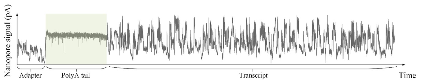
The normalization remains robust with variable poly(A) tail lengths, as long as the poly(A) region is sufficiently long. The linker sequence will be assigned to the adapter part rather than the poly(A) part.
To improve clarity in the revised manuscript, we have added the following explanation:
“Due to inherent variability between nanopores in the sequencing device, the baseline levels and standard deviations of k-mer signals can differ across reads, even for the same transcript. To standardize the signal for downstream analyses, we extract the raw current signal segments corresponding to the poly(A) tail of each read. Since the poly(A) tail provides a stable reference, we normalize the raw current signals across reads, ensuring that the mean and standard deviation of the poly(A) tail are consistent across all reads. This step is crucial for reducing…..”
We chose to use the poly(A) tail for normalization because it is sequence-invariant—i.e., all poly(A) tails consist of identical k-mers, unlike transcript sequences which vary in composition. In contrast, using the transcript region for normalization can introduce biases: for instance, reads with more diverse k-mers (having inherently broader signal distributions) would be forced to match the variance of reads with more uniform k-mers, potentially distorting the baseline across k-mers.
Page 7, 5mer parameter table: r9.4_180mv_70bps_5mer_RNA is an older kmer model (>2 years). How does your method perform with the newer RNA kmer models that do permit the detection of multiple ribonucleotide modifications? Addressing this comment is crucial because it is feasible that SegPore will underperform in comparison to the newer RNA base caller models (requiring the use of RNA004 datasets).
Thank you for highlighting this important point. For RNA004, we have updated SegPore to ensure compatibility with the latest kit. In our revised manuscript, we demonstrate that the translocation-based segmentation hypothesis remains valid for RNA004, as supported by new analyses presented in the supplementary Figure S4.
Additionally, we performed a new benchmark with f5c and Uncalled4 in RNA004 data in the revised manuscript (Table 2), where SegPore exhibit a better performance than f5c and Uncalled4.
We agree that benchmarking against the latest Dorado models—specifically rna004_130bps_hac@v5.1.0 and rna004_130bps_sup@v5.1.0, which include built-in modification detection capabilities—would provide valuable context for evaluating the utility of SegPore. However, generating a comprehensive k-mer parameter table for RNA004 requires a large, well-characterized dataset. At present, such data are limited in the public domain. Additionally, Dorado is developed by ONT and its internal training data have not been released, making direct comparisons difficult.
Our current focus is on improving raw signal segmentation quality, which are upstream tasks critical to many downstream analyses, including RNA modification detection. Future work may include benchmarking SegPore against models like Dorado once appropriate data become available.
The Methods and Results sections contain redundant information - please streamline the information in these sections and reduce the redundancy. For example, the benchmarking section may be better situated in the Results section.
Following your advice, we have removed redundant texts about the Segmentation benchmark from Materials and Methods in the revised manuscript.
Minor comments
(1) Introduction
Page 3: "By incorporating these dynamics into its segmentation algorithm...". Please provide an example of how motor protein dynamics can impact RNA translocation. In particular, please elaborate on why motor protein dynamics would impact the translocation of modified ribonucleotides differently to canonical ribonucleotides. This is provided in the results, but please also include details in the Introduction.
Following your advice, we added one sentence to explain how the motor protein affect the translocation of the DNA/RNA molecule in the revised manuscript.
“This observation is also supported by previous reports, in which the helicase (the motor protein) translocates the DNA strand through the nanopore in a back-and-forth manner. Depending on ATP or ADP binding, the motor protein may translocate the DNA/RNA forward or backward by 0.5-1 nucleotides.”
As far as we understand, this translocation mechanism is not specific to modified or unmodified nucleotides. For further details, we refer the reviewer to the original studies cited.
Page 3: "This lack of interpretability can be problematic when applying these methods to new datasets, as researchers may struggle to trust the predictions without a clear understanding of how the results were generated." Please provide details and citations as to why researchers would struggle to trust the predictions of m6Anet. Is it due to a lack of understanding of how the method works, or an empirically demonstrated lack of reliability?
Thank you for pointing this out. The lack of interpretability in deep learning models such as m6Anet stems primarily from their “black-box” nature—they provide binary predictions (modified or unmodified) without offering clear reasoning or evidence for each call.
When we examined the corresponding raw signals, we found it difficult to visually distinguish whether a signal segment originated from a modified or unmodified ribonucleotide. The difference is often too subtle to be judged reliably by a human observer. This is illustrated in the newly added Supplementary Figure S5, which shows Nanopolish-aligned raw signals for the central 5mer GGACT in Figure 4B, displayed both uncolored and colored by modification state (according to the ground truth).
Although deep neural networks can learn subtle, high-dimensional patterns in the signal that may not be readily interpretable, this opacity makes it difficult for researchers to trust the predictions—especially in new datasets where no ground truth is available. The issue is not necessarily an empirically demonstrated lack of reliability, but rather a lack of transparency and interpretability.
We have updated the manuscript accordingly and included Supplementary Figure S5 to illustrate the difficulty in interpreting signal differences between modified and unmodified states.
Page 3: "Instead of relying on complex, opaque features...". Please provide evidence that the research community finds the figures generated by m6Anet to be difficult to interpret, or delete the sections relating to its perceived lack of usability.
See the figure provided in the response to the previous point. We added a reference to this figure in the revised manuscript.
“Instead of relying on complex, opaque features (see Supplementary Figure S5), SegPore leverages baseline current levels to distinguish between…..”
(2) Materials and Methods
Page 5, Preprocessing: "We begin by performing basecalling on the input fast5 file using Guppy, which converts the raw signal data into base sequences.". Please change "base" to ribonucleotide.
Revised as requested.
Page 5 and throughout, please refer to poly(A) tail, rather than polyA tail throughout.
Revised as requested.
Page 5, Signal segmentation via hierarchical Hidden Markov model: "...providing more precise estimates of the mean and variance for each base block, which are crucial for downstream analyses such as RNA modification prediction." Please specify which method your HHMM method improves upon.
Thank you for the suggestion. Since this section does not include a direct comparison, we revised the sentence to avoid unsupported claims. The updated sentence now reads:
"...providing more precise estimates of the mean and variance for each base block, which are crucial for downstream analyses such as RNA modification prediction."
Page 10, GMM for 5mer parameter table re-estimation: "Typically, the process is repeated three to five times until the 5mer parameter table stabilizes." How is the stabilisation of the 5mer parameter table quantified? What is a reasonable cut-off that would demonstrate adequate stabilisation of the 5mer parameter table?
Thank you for the comment. We assess the stabilization of the 5mer parameter table by monitoring the change in baseline values across iterations. If the absolute change in baseline values for all 5mers is less than 1e-5 between two consecutive iterations, we consider the estimation to have stabilized.
Page 11, M6A site level benchmark: why were these datasets selected? Specifically, why compare human and mouse ribonuclotide modification profiles? Please provide a justification and a brief description of the experiments that these data were derived from, and why they are appropriate for benchmarking SegPore.
Thank you for the comment. These data are taken from a previous benchmark studie about m6A estimation from RNA002 data in the literature (https://doi.org/10.1038/s41467-023-37596-5). We think the data are appropreciate here.
Thank you for the comment. The datasets used were taken from a previous benchmark study on m6A estimation using RNA002 data (https://doi.org/10.1038/s41467-023-37596-5). These datasets include human and mouse transcriptomes and have been widely used to evaluate the performance of RNA modification detection tools. We selected them because (i) they are based on RNA002 chemistry, which matches the primary focus of our study, and (ii) they provide a well-characterized and consistent benchmark for assessing m6A detection performance. Therefore, we believe they are appropriate for validating SegPore.
(3) Results
Page 13, RNA translocation hypothesis: "The raw current signals, as shown in Fig. 1B...". Please check/correct figure reference - Figure 1B does not show raw current signals.
Thank you for pointing this out. The correct reference should be Figure 2B. We have updated the figure citation accordingly in the revised manuscript.
Page 19, m6A identification at the site level: "For six selected m6A motifs, SegPore achieved an ROC AUC of 82.7% and a PR AUC of 38.7%, earning the third best performance compared with deep leaning methods m6Anet and CHEUI (Fig. 3D)." SegPore performs third best of all deep learning methods. Do the authors recommend its use in conjunction with m6Anet for m6A detection? Please clarify in the text.
This sentence aims to convey that SegPore alone can already achieve good performance. If interpretability is the primary goal, we recommend using SegPore on its own. However, if the objective is to identify more potential m6A sites, we suggest using the combined approach of SegPore and m6Anet. That said, we have chosen not to make explicit recommendations in the main text to avoid oversimplifying the decision or potentially misleading readers.
Page 19, m6A identification at the single molecule level: "one transcribed with m6A and the other with normal adenosine". I assume that this should be adenine? Please replace adenosine with adenine throughout.
Thank you for pointing this out. We have revised the sentence to use "adenine" where appropriate. In other instances, we retain "adenosine" when referring specifically to adenine bound to a ribose sugar, which we believe is suitable in those contexts.
Page 19, m6A identification at the single molecule level: "We used 60% of the data for training and 40% for testing". How many reads were used for training and how many for testing? Please comment on why these are appropriate sizes for training and testing datasets.
In total, there are 1.9 million reads, with 1.14 million used for training and 0.76 million for testing (60% and 40%, respectively). We chose this split to ensure that the training set is sufficiently large to reliably estimate model parameters, while the test set remains substantial enough to robustly evaluate model performance. Although the ratio was selected somewhat arbitrarily, it balances the need for effective training with rigorous validation.
(4) Discussion
Page 21: "We believe that the de-noised current signals will be beneficial for other downstream tasks." Which tasks? Please list an example.
We have revised the text for clarity as follows:
“We believe that the de-noised current signals will be beneficial for other downstream tasks, such as the estimation of m5C, pseudouridine, and other RNA modifications.”
Page 22: "One can generally observe a clear difference in the intensity levels between 5mers with a m6A and normal adenosine, which is easier for human to interpret if a predicted m6A site is real." This statement is vague and requires qualification. Please reference a study that demonstrates the human ability to interpret two similar graphs, and demonstrate how it relates to the differences observed in your data.
We apologize for the confusion. We have revised the sentence as follows:
“One can generally observe a clear difference in the intensity levels between 5mers with an m6A and those with a normal adenosine, which makes it easier for a researcher to interpret whether a predicted m6A site is genuine.”
We believe that Figures 3A, 3B, and 4B effectively illustrate this concept.
Page 23: How long does SegPore take for its analyses compared to other similar tools? How long would it take to analyse a typical dataset?
We have added run-time statistics for datasets of varying sizes in the revised manuscript (see Supplementary Figure S6). This figure illustrates SegPore’s performance across different data volumes to help estimate typical processing times.
(5) Figures
Figure 4C. Please number the hierachical clusters and genomic locations in this figure. They are referenced in the text.
Following your suggestion, we have labeled the hierarchical clusters and genomic locations in Figure 4C in the revised manuscript.
In addition, we revised the corresponding sentence in the main text as follows: “Biclustering reveals that modifications at g6 are specific to cluster C4, g7 to cluster C5, and g8 to cluster C6, while the first five genomic locations (g1 to g5) show similar modification patterns across all reads.”
-
-
rori.figshare.com rori.figshare.com
-
Reviewer #3 (Public review):
Summary:
This paper investigates the Matthew effect, where early success in funding peer review can translate into potentially unwarranted later success. It also investigated the previously found "setback" effect for those who narrowly miss out on funding.
Strengths:
The study used data from six funding agencies, which increases the generalisability, and was able to link bibliographic data for around 95% of applicants. The authors nicely illustrate how the previously found "setback" effect for near-miss applicants could be a collider bias due to those who chose to apply sometime later. This is a good explanation for the counter-intuitive effect and is nicely shown in Figure 5.
Weaknesses:
Most of the methods were clearly presented, but I have a few questions and comments, as outlined below.
In Figure 4(a) why are the "post" means much lower than the "pre"? This contradicts the expected research trajectory of researchers. Or is this simply due to less follow-up time? But doesn't the field citation ratio control for follow-up time?
The choice of the log-normal distribution for latent quality was not entirely clear to me. This would create some skew, rather than a symmetric distribution, which may be reasonable but log-normal distributions can have a very long tail which might not mimic reality, as I would not expect a small number of researchers to be extremely above the crowd. However, then the skew was potentially dampened by using percentile scores. Some further reasoning and plots of the priors would help.
Can the authors confirm the results of Figure S9 which show no visible effect of altering the standard deviation for the review parameter or the mean citations? Is this just because the prior for quality is dominated by the data? Could it be that the width of the distribution for quality does not matter, as it's the relative difference/ranking that counts? So the beta in equation 6 changes to adjust to the different quality scale?
The contrary result for the FWF is not explained (Table S3). Does this funder have different rules around re-applicants or many other competing funders?
The outlined qualitative research sounds worthwhile. Another potential mechanism (based on anecdote) is that some researchers react irrationally to rejection or acceptance, tending to think that the whole agency likes or hates their work based on one experience. Many researchers do not appreciate that it was a somewhat random selection of reviewers who viewed their work, and it will unlikely be the same reviewers next time.
"A key implication is the importance of encouraging promising, but initially unsuccessful applicants to reapply." Yes, A policy implication is to give people multiple chances to be lucky, perhaps by giving fewer grants to more people, which could be achieved by shortening the funding period (e.g., 4 year fellowships instead of 5 years). Although this will have some costs as applicants would need to spend more time on applications and suffer increased stress of shorter-term contracts. The bridge grants is potentially an ideal half-way house between many short-term and few long-term awards. Giving more grants to fewer people is supported by this analysis showing a diminishing returns in research outputs with more funding, DOI: 10.1371/journal.pone.0065263.
Making more room for re-applicants also made me wonder if there should be an upper cap on funding, potentially for people who have been incredibly successful. Of course, funders generally want to award successful researchers, but people who've won over some limit, for example $50 million, could likely be expected to win funding from other sources such as philanthropy and business. Graded caps could occur by career stage.
-
-
socialsci.libretexts.org socialsci.libretexts.org
-
In India, cows also act as an essential source of fertilizer, to the tune of 700 million tons of manure annually, about half of which is used for fertilizer and the other half of which is used as fuel for cooking.
I never knew that's as one their way to use cows
-
- Sep 2025
-
www.news-medical.net www.news-medical.net
-
Dengue fever,
some UN facts: Dengue is a viral infection caused by the dengue virus (DENV), which is transmitted to humans through the bite of infected mosquitoes. About half of the world's population is now at risk of dengue, with an estimated 100–400 million infections occurring each year. Dengue is found in tropical and sub-tropical climates worldwide, mostly in urban and semi-urban areas. While many DENV infections are asymptomatic or produce only mild illness, DENV can occasionally cause more severe cases, and even death. Prevention and control of dengue rely on vector control. There is no specific treatment for dengue/severe dengue, and early detection and access to proper medical care greatly lower fatality rates of severe dengue.
-
-
climateinstitute.ca climateinstitute.ca
-
So far in 2025, wildfires have consumed a total area of 8.7 million hectares, over two and half times the size of Vancouver Island. Communities not typically known for wildfire activity, including in Atlantic Canada, now face record drought conditions and increasing fire risks.
This part is already strong because it compares the wildfire area to something familiar (Vancouver Island). That’s a smart accessibility choice because it makes an abstract number (8.7 million hectares) much easier to picture. This supports the Perceivable principle, the information becomes more meaningful by using a relatable example. It’s a reminder that context is key when designing acce
-
QUICK FACTS Canada’s emissions in 2024 are estimated at 694 megatonnes of carbon dioxide-equivalent (Mt), or 8.5 per cent below 2005 levels. Oil and gas: Emissions rose 1.9 per cent from the previous year, driven by a 3.4 per cent increase in oil sands emissions. Transportation: Emissions dropped 0.7 per cent, continuing a modest downward trend from 2023. Buildings: Emissions declined 1.2 per cent, a slower pace than the previous year due to a colder winter. Heavy industry: Emissions fell 1.2 per cent, showing signs of decarbonization progress despite uneven results across sub-sectors. Electricity: Emissions dropped 1.9 per cent to 59 per cent below 2005 levels, reinforcing the importance of coordinated federal and provincial policy and technology improvements. Climate change makes wildfires bigger, hotter, and more frequent. So far in 2025, wildfires have consumed a total area of 8.7 million hectares, over two and half times the size of Vancouver Island. Communities not typically known for wildfire activity, including in Atlantic Canada, now face record drought conditions and increasing fire risks. Damages from extreme weather events in 2024 shattered records for the costliest year in Canada, at more than $8.5 billion in insured losses.
I think the “Quick Facts” section is a great accessibility feature. Using bullet points makes the information clear, scannable, and easy to navigate for readers and screen readers alike. It shows good use of the Perceivable principle because the structure allows key numbers to stand out instead of being buried in long paragraphs. More pages should use this kind of format for presenting data.
-
-
-
Attention: Prior to this page note, "This is a Subscriber Exclusive story." Now it is free to anybody using Hypothesis.
Hamady grocery store closing its doors on Flint's north end
Published: Nov. 06, 2018, 11:01 p.m.
FLINT, MI - Jim McColgan Jr. spent the last two and a half years of his life working to open up Hamady Complete Food Centers on Flint's north side.
The store near the corner of Clio and Pierson roads in the Hallwood Plaza opened July 25, teeming with nostalgia including the paper sacks Hamady came to be known by many in the community and the promise of 80-plus jobs.
But the rebirth of the store was short lived.
McColgan Jr., the store's owner, confirmed the location will close Tuesday, Nov. 6, less than four months after it launched anew.
"It's just a sad day in my personal life and in also in the life of Flint and the north end community," he said Tuesday evening. "I really wanted to build a beautiful store here. I just wanted it to go that way and everybody to just shop and enjoy themselves and it's just very sad."
He thanked the city of Flint, Mayor Karen Weaver, and the local chamber of commerce for their "wonderful" support along the way, but McColgan Jr. added, "We just didn't have enough traffic, enough community support."
The Hamady Bros. supermarket chain started in 1911 with a small store on East Dayton Street and Industrial Avenue in Flint.
Michael Hamady and his cousin Kamol Hamady co-founded the chain, which grew to 37 stores in the Flint area, employed approximately 1,300 people, and at one point generated $100 million in annual revenue, according to Flint Journal records.
Alex Dandy took over the business in 1974, and workers took part in a seven-week strike in 1987. Dandy served time in prison for tax evasion and fraud when he took millions from Hamady and another supermarket company.
James M. McColgan Sr., under a reorganization plan, ran the Hamady's chain in 1988. A year later, the court approved the sale of Hamady to McColgan. When the company's losses exceeded $2 million in 1991, McColgan Sr. decided to sell the chain, according to Journal records. He filed for bankruptcy in May 1991 and last Hamady store closed two months later.
McColgan Jr. took pride in bringing back the name, which he commented still holds some high esteem in the Flint community.
"Hamady is a Flint icon. Everybody remembers Hamady. Even younger kids, even younger people," he previously said. "Hamady is still a drawing force in the city of Flint. I am very proud and honored to be a part of the Hamady family and the Hamady name."
Some delays took place in the opening process, including a stop-work order issued in late March due to Hamady working without proper permits.
In the face of the closure, McColgan Jr. tried to remain upbeat but added the discussion with employees was a difficult one.
"It was very tearful. The employees were very emotional," he commented of the situation. "Everybody that worked here put their life into this store. We are all just going to be positive and move forward."
When asked about potential additional stores as had been discussed for Clio, Durand, Holly, and South Saginaw Street in Flint, McColgan noted: "You never know what the future is going to hold, but I'm young and I'm not ready to retire."
-
-
www.biorxiv.org www.biorxiv.org
-
Author response:
The following is the authors’ response to the previous reviews
Reviewer #1 (Public review):
I still have a bone to pick with the claim that "activity-dependent changes in channel voltage-dependence alone are insufficient to attain bursting". As I mentioned in my previous comment, this is also the case for the gmax values (channel density). If you choose the gmax's to be in a reasonable range, then the statement above is simply cannot be true. And if, in contrast, you choose the activation/inactivation parameters to be unreasonable, then no set of gmax's can produce proper activity. So I remain baffled what exactly is the point that the authors are trying to make.
We thank the reviewer for this clarification. We did not intend to imply that voltage-dependence modulation is universally incapable of supporting bursting or that conductance changes alone are universally sufficient. To avoid any overstatement, we now write:
“…activity-dependent changes in channel voltage-dependence alone did not assemble bursting from these low-conductance initial states (cf. Figure 1B)”.
Reviewer #2 (Public review):
(1) The main question not addressed in the paper is the relative efficiency and/or participation of voltage-dependence regulation compared to channel conductance in achieving the expected pattern of activity. Is voltage-dependence participating to 50% or 10%. Although this is a difficult question to answer (and it might even be difficult to provide a number), it is important to determine whether channel conductance regulation remains the main parameter allowing the achievement of a precise pattern of activity (or its recovery after perturbation).
We appreciate the reviewer’s interest in a quantitative partitioning of the contributions from voltage-dependence regulation versus conductance regulation. We agree that this would be an important analysis in principle. In practice, obtaining this would be difficult.
Our goal here was to establish the principle: that half-(in)activation shifts can meaningfully influence recovery. This is not an obvious result, given that these two processes can act on vastly different timescales.
That said, our current dataset does provide partial quantitative insight. Eight of the twenty models required some form of voltage-dependence modulation to recover; among these, two only recovered under fast modulation and two only under slow modulation. This demonstrates that voltage-dependence regulation is essential for recovery in some neurons, and its timescale critically shapes the outcome.
(2) Another related question is whether the speed of recovery is significantly modified by implemeting voltage-dependence regulation (it seems to be the case looking at Figure 3). More generally, I believe it would be important to give insights into the overall benefit of implementing voltage-dependence regulation, beyond its rather obvious biological relevance.
Our current results suggest that voltage-dependence regulation can indeed accelerate recovery, as illustrated in Figure 3 and supported by additional simulations (not shown). However, a fully quantitative comparison (e.g., time-to-recovery distributions or survival analysis) would require a much larger ensemble of degenerate models to achieve sufficient statistical power across all four conditions. Generating and simulating this expanded model set is computationally intensive, requiring stochastic searches in a high-dimensional parameter space, full time-course simulations, and a subsequent selection process that may succeed or fail.
The principal aim of the present study is conceptual: to demonstrate that this multi-timescale homeostatic model—built here for the first time—can capture interactions between conductance regulation and voltage-dependence modulation during assembly (“neurodevelopment”) and perturbation. Establishing the conceptual framework and exploring its qualitative behavior were the necessary first steps before pursuing a large-scale quantitative study.
(3) Along the same line, the conclusion about how voltage-dependence regulation and channel conductance regulation interact to provide the neuron with the expected activity pattern (summarized and illustrated in Figure 6) is rather qualitative. Consistent with my previous comments, one would expect some quantitative answers to this question, rather than an illustration that approximately places a solution in parameter space.
We appreciate the reviewer’s interest in a more quantitative characterization of the interaction between voltage-dependence and conductance regulation (Fig. 6). As noted in our responses to Comments 1 and 2, some of the facets of this interaction—such as the ability to recover from perturbations and the speed of assembly—can be measured.
However, fully quantifying the landscape sketched in Figure 6 would require systematically mapping the regions of high-dimensional parameter space where stable solutions exist. In our model, this space spans 18 dimensions (maximal conductances and half‑(in)activations). Even a coarse grid with three samples per dimension would entail over 100 million simulations, which is computationally prohibitive and would still collapse to a schematic representation for visualization.
For this reason, we chose to present Figure 6 as a conceptual summary, illustrating the qualitative organization of solutions and the role of multi-timescale regulation, rather than attempting an exhaustive mapping. We view this figure as a necessary first step toward guiding future, more quantitative analyses.
Reviewer #3 (Public review):
Mondal et al. use computational modeling to investigate how activity-dependent shifts in voltage-dependent (in)activation curves can complement changes in ion channel conductance to support homeostatic plasticity. While it is well established that the voltage-dependent properties of ion channels influence neuronal excitability, their potential role in homeostatic regulation, alongside conductance changes, has remained largely unexplored. The results presented here demonstrate that activity-dependent regulation of voltage dependence can interact with conductance plasticity to enable neurons to attain and maintain target activity patterns, in this case, intrinsic bursting. Notably, the timescale of these voltage-dependent shifts influences the final steady-state configuration of the model, shaping both channel parameters and activity features such as burst period and duration. A major conclusion of the study is that altering this timescale can seamlessly modulate a neuron's intrinsic properties, which the authors suggest may be a mechanism for adaptation to perturbations.
While this conclusion is largely well-supported, additional analyses could help clarify its scope. For instance, the effects of timescale alterations are clearly demonstrated when the model transitions from an initial state that does not meet the target activity pattern to a new stable state. However, Fig. 6 and the accompanying discussion appear to suggest that changing the timescale alone is sufficient to shift neuronal activity more generally. It would be helpful to clarify that this effect primarily applies during periods of adaptation, such as neurodevelopment or in response to perturbations, and not necessarily once the system has reached a stable, steady state. As currently presented, the simulations do not test whether modifying the timescale can influence activity after the model has stabilized. In such conditions, changes in timescale are unlikely to affect network dynamics unless they somehow alter the stability of the solution, which is not shown here. That said, it seems plausible that real neurons experience ongoing small perturbations which, in conjunction with changes in timescale, could allow gradual shifts toward new solutions. This possibility is not discussed but could be a fruitful direction for future work.
We thank the reviewer for this thoughtful comment and for highlighting an important point about the scope of our conclusions regarding timescale effects. The reviewer is correct that our simulations demonstrate the influence of voltage-dependence timescale primarily during periods of adaptation—when the neuron is moving from an initial, target-mismatched state toward a final target-satisfying state. Once the system has reached a stable solution, simply changing the timescale of voltage-dependent modulation does not by itself shift the neuron’s activity, unless a new perturbation occurs that re-engages the homeostatic mechanism. We have clarified this point in the revised Discussion.
The confusion likely arose from imprecise phrasing in the original text describing Figure 6. Previously, we wrote:
“When channel gating properties are altered quickly in response to deviations from the target activity, the resulting electrical patterns are shown in Figure 6 as the orange bubble labeled 𝝉<sub>𝒉𝒂𝒍𝒇</sub> = 6 s”.
We have revised this sentence to emphasize that the orange bubble represents the eventual stable state, rather than implying that timescale changes alone drive activity shifts:
”When channel gating properties are altered quickly in response to deviations from the target activity, the neuron ultimately settles into a stable activity pattern. The resulting electrical patterns are shown in Figure 6 as the orange bubble labeled 𝝉<sub>𝒉𝒂𝒍𝒇</sub> = 6 s”.
Reviewer #1 (Recommendations for the authors):
Unless I am missing something, Figure 2 should be a supplement to Figure 1. I would prefer to see panel B in Figure 1 to indicate that the findings of that figure are general. Panel A really is not showing anything useful to the reader.
We appreciate the suggestion to combine Figure 2 with Figure 1, but we believe keeping Figure 2 separate better preserves the manuscript’s flow. Figure 1 illustrates the mechanism in a single model, while Figure 2 presents the population-level summary that generalizes the phenomenon across all models.
Also, I find Figure 6 unnecessary and its description in the Discussion more detracting than useful. Even with the descriptions, I find nothing in the figure itself that clarifies the concept.
We appreciate the reviewer’s feedback on Figure 6. The purpose of this figure is to conceptually illustrate that multiple degenerate solutions can satisfy the calcium target and that the timescale of voltage‑dependence modulation can influence which region of this solution space is accessed during the acquisition of the activity target. Reviewer 3 noted some confusion about this point. We made a small clarifying edit.
At the risk of being really picky, I also don't see the purpose of Figure 7. And I find it strange to plot -Vm just because that's the argument of findpeaks.
We appreciate the reviewer’s comment on Figure 7. The purpose of this figure is to illustrate exactly what the findpeaks function is detecting, as indicated by the red arrows on the traces. For readers unfamiliar with findpeaks, it may not be obvious how the algorithm interprets the waveform. Showing the peaks directly ensures that the measurements used in our analysis align with what one would intuitively expect.
Reviewer #2 (Recommendations for the authors):
The writing of the article has been much improved since the last version. It is much clearer, and the discussion has been improved and better addresses the biological foundations and relevance of the study. However, conclusions are rather qualitative, while one would expect some quantitative answers to be provided by the modeling approach.
We appreciate the reviewer’s concern regarding quantification and share this perspective. As noted above, our study is primarily conceptual. Many aspects of the model, such as calcium handling and channel regulation, are parameterized based on incomplete biological data. These uncertainties make robust quantitative predictions difficult, so we focus on qualitative outcomes that are likely to hold independently of specific parameter choices.
-
-
www.theguardian.com www.theguardian.com
-
“humanisers”, such as CopyGenius and StealthGPT, the latter which boasts that it can produce undetectable content and claims to have helped half a million students produce nearly 5m papers.
This is actually really alarming! Wow!
-
-
mlpp.pressbooks.pub mlpp.pressbooks.pub
-
hese service industries profited from the mining boom: as failed prospectors found, the rush itself often generated more wealth than the mines. The $25.5 million in gold that left Colorado in the first seven years after the Pikes Peak gold strike, for example, was less than half of what speculators had invested in the fever.
The mining boom often enriched service industries still as the rush generated massive speculation. In Colorado, the gold extracted was less than half of what investors poured into it..
-
-
mlpp.pressbooks.pub mlpp.pressbooks.pub
-
Nearly 100 Americans died in “The Great Upheaval.” Workers destroyed nearly $40 million worth of property. The strike galvanized the country. It convinced laborers of the need for institutionalized unions, persuaded businesses of the need for even greater political influence and government aid, and foretold a half century of labor conflict in the United States.
The fact that workers had to come to such drastic measures just to get a voice in what they're paid, or even reduced work hours. They had to destroy nearly $40 million dollars (about $1,174,720,000 today) worth of property, and there were many casualties. It makes me thankful that we have the unions we have today, but also wonder what would happen if something like this happened in modern days. Would it be as catastrophic, or would the government avoid all of it by complying?
-
- Aug 2025
-
www.americanyawp.com www.americanyawp.com
-
Many of these ancillary operations profited from the mining boom: as failed prospectors found, the rush itself often generated more wealth than the mines. The gold that left Colorado in the first seven years after the Pikes Peak gold strike—estimated at $25.5 million—was, for instance, less than half of what outside parties had invested in the fever. The 100,000-plus migrants who settled in the Rocky Mountains were ultimately more valuable to the region’s development than the gold they came to find.
Sometimes it's more of the sizzle than the steak.
-
-
apjjf.org apjjf.org
-
spring of 1953, the Air Force targeted irrigation dams on the Yalu River, both to destroy the North Korean rice crop and to pressure the Chinese, who would have to supply more food aid to the North. Five reservoirs were hit, flooding thousands of acres of farmland, inundating whole towns and laying waste to the essential food source for millions of North Koreans.10
majority of 3 million killed in the north even tho they had half the population of the south
USAF targeted irrigation dams on the Yalu River (spring 1953) to destroy rice crops. They hit 5 reservoirs which flooded thousands of acres of farmland, making it unusable. Essential food source, affected millions of North Koreans
-
- Jul 2025
-
arxiv.org arxiv.org
-
Overview
This manuscript provides an in-depth examination of the use of initials versus full names in academic publications over time, identifying what the authors term the "Initial Era" (1945-1980) as a period during which initials were predominantly used. The authors contextualize this within broader technological, cultural, and societal changes, leveraging a large dataset from the Dimensions database. This study contributes to the understanding of how bibliographic metadata reflects shifts in research culture.
Strengths
+ Novel concept and historical depth
The paper introduces a unique angle on the evolution of scholarly communication by focusing on the use of initials in author names. The concept of the "Initial Era" is original and well- defined, adding a historical dimension to the study of metadata that is often overlooked. The manuscript provides a compelling narrative that connects technological changes with shifts in academic culture.
+ Comprehensive dataset
The use of the Dimensions database, which includes over 144 million publications, lends significant weight to the findings. The authors effectively utilize this resource to provide both anecdotal and statistical analyses, giving the paper a broad scope. The differentiation between the anecdotal and statistical epochs helps clarify the limitations of the dataset and strengthens the authors' conclusions.
+ Cross-disciplinary relevance
The study's insights into the sociology of research, particularly the implications of name usage for gender and cultural representation, are highly relevant across multiple disciplines. The paper touches on issues of diversity, bias, and the visibility of researchers from different backgrounds, making it an important contribution to ongoing discussions about equity in academia.
+ Technological impact
The authors successfully connect the decline of the "Initial Era" to the rise of digital publishing technologies, such as Crossref, PubMed, and ORCID. This link between technological infrastructure and shifts in scholarly norms is a critical insight, showing how the adoption of new tools has real-world implications for academic practices.
Weaknesses
- Lack of clarity and readability
While the manuscript is rich in data and analysis, it can be dense and challenging to follow for readers not familiar with the technical details of bibliometric studies. The text occasionally delves into highly specific discussions that may be difficult for a broader audience to grasp while other concepts are introduced in cursory. Consider condensing the introduction section, removing unrelated historical accounts, and leading the audience to the key objectives of this research much earlier.
- Missing empirical case studies
The manuscript remains largely theoretical, relying heavily on data analysis without providing concrete case studies or empirical examples of how the "Initial Era" affected individual disciplines or researchers. A more detailed exploration of specific instances where the use of initials had significant consequences would make the findings more tangible. Incorporating case studies or anecdotes from the history of science that illustrate the real-world impacts of the trends identified in the data would enrich the paper. These examples could help ground the analysis in practical outcomes and demonstrate the relevance of the "Initial Era" to contemporary debates.
- Half-baked comparative analysis
Although the paper presents interesting data about different countries and disciplines, the comparative analysis between these groups could be further developed. For example, the reasons behind the differences in initial use between countries with different writing systems or academic cultures are not fully explored. A more in-depth comparative analysis that explains the cultural, linguistic, or institutional factors driving the observed differences in initial use would add nuance to the findings. This could involve a more detailed discussion of how non-Roman writing systems influence name formatting or how specific national academic policies shape author metadata.
- Limited discussion of alternative explanations
While the authors link the decline of the "Initial Era" to technological advancements, other potential explanations, such as changing editorial policies (“technological harmonisation”), shifts in academic prestige, or the influence of global collaboration, are not fully explored. The paper could benefit from a broader discussion of these factors. Expanding the discussion to include alternative explanations for the decline of initial use, and how these might interact with technological changes, would provide a more comprehensive view. Engaging with literature on academic publishing practices, editorial decisions, and global research trends could help contextualize the findings within a wider framework.
Conclusion
This manuscript offers a novel and insightful analysis of the evolution of name usage in academic publications, providing valuable contributions to the fields of bibliometrics, science studies, and research culture. With improvements in clarity, comparative analysis, and the incorporation of case studies, this paper has the potential to make a significant impact on our understanding of how metadata reflects broader societal and technological changes in academia. The authors are encouraged to refine their discussion and expand on the implications of their findings to make the manuscript more accessible and applicable to a wider audience.
-
-
www.medrxiv.org www.medrxiv.org
-
Author response:
The following is the authors’ response to the original reviews
Public Reviews:
Reviewer #1 (Public Review):
Summary:
In this manuscript, the authors provide a study among healthy individuals, general medical patients and patients receiving haematopoietic cell transplants (HCT) to study the gut microbiome through shotgun metagenomic sequencing of stool samples. The first two groups were sampled once, while the patients receiving HCT were sampled longitudinally. A range of metadata (including current and previous (up to 1 year before sampling) antibiotic use) was recorded for all sampled individuals. The authors then performed shotgun metagenomic sequencing (using the Illumina platform) and performed bioinformatic analyses on these data to determine the composition and diversity of the gut microbiota and the antibiotic resistance genes therein. The authors conclude, on the basis of these analyses, that some antibiotics had a large impact on gut microbiota diversity, and could select opportunistic pathogens and/or antibiotic resistance genes in the gut microbiota.
Strengths:
The major strength of this study is the considerable achievement of performing this observational study in a large cohort of individuals. Studies into the impact of antibiotic therapy on the gut microbiota are difficult to organise, perform and interpret, and this work follows state-of-the-art methodologies to achieve its goals. The authors have achieved their objectives and the conclusion they draw on the impact of different antibiotics and their impact on the gut microbiota and its antibiotic resistance genes (the 'resistome', in short), are supported by the data presented in this work.
Weaknesses:
The weaknesses are the lack of information on the different resistance genes that have been identified and which could have been supplied as Supplementary Data.
We have now supplied a list of individual resistance genes as supplementary data.
In addition, no attempt is made to assess whether the identified resistance genes are associated with mobile genetic elements and/or (opportunistic) pathogens in the gut. While this is challenging with short-read data, alternative approaches like long-read metagenomics, Hi-C and/or culture-based profiling of bacterial communities could have been employed to further strengthen this work.
We agree this is a limitation, and we now refer to this in the discussion. Unfortunately we did not have funding to perform additional profiling of the samples that would have provided more information about the genetic context of the AMR genes identified.
Unfortunately, the authors have not attempted to perform corrections for multiple testing because many antibiotic exposures were correlated.
The reviewer is correct that we did not perform formal correction for multiple testing. This was because correlation between antimicrobial exposures meant we could not determine what correction would be appropriate and not overly conservative. We now describe this more clearly in the statistical analysis section.
Impact:
The work may impact policies on the use of antibiotics, as those drugs that have major impacts on the diversity of the gut microbiota and select for antibiotic resistance genes in the gut are better avoided. However, the primary rationale for antibiotic therapy will remain the clinical effectiveness of antimicrobial drugs, and the impact on the gut microbiota and resistome will be secondary to these considerations.
We agree that the primary consideration guiding antimicrobial therapy will usually be clinical effectiveness. However antimicrobial stewardship to minimise microbiome disruption and AMR selection is an increasingly important consideration, particularly as choices can often be made between different antibiotics that are likely to be equally clinically effective.
Reviewer #2 (Public Review):
Summary:
In this manuscript by Peto et al., the authors describe the impact of different antimicrobials on gut microbiota in a prospective observational study of 225 participants (healthy volunteers, inpatients and outpatients). Both cross-sectional data (all participants) and longitudinal data (a subset of 79 haematopoietic cell transplant patients) were used. Using metagenomic sequencing, they estimated the impact of antibiotic exposure on gut microbiota composition and resistance genes. In their models, the authors aim to correct for potential confounders (e.g. demographics, non-antimicrobial exposures and physiological abnormalities), and for differences in the recency and total duration of antibiotic exposure. I consider these comprehensive models an important strength of this observational study. Yet, the underlying assumptions of such models may have impacted the study findings (detailed below). Other strengths include the presence of both cross-sectional and longitudinal exposure data and the presence of both healthy volunteers and patients. Together, these observational findings expand on previous studies (both observational and RCTs) describing the impact of antimicrobials on gut microbiota.
Weaknesses:
(1) The main weaknesses result from the observational design. This hampers causal interpretation and corrects for potential confounding necessary. The authors have used comprehensive models to correct for potential confounders and for differences between participants in duration of antibiotic exposure and time between exposure and sample collection. I wonder if some of the choices made by the authors did affect these findings. For example, the authors did not include travel in the final model, but travel (most importantly, south Asia) may result in the acquisition of AMR genes [Worby et al., Lancet Microbe 2023; PMID 37716364). Moreover, non-antimicrobial drugs (such as proton pump inhibitors) were not included but these have a well-known impact on gut microbiota and might be linked with exposure to antimicrobial drugs. Residual confounding may underlie some of the unexplained discrepancies between the cross-sectional and longitudinal data (e.g. for vancomycin).
We agree that the observational design means there is the potential for confounding, which, as the reviewer notes, we attempt to account for as far as possible in the multivariable models presented. We cannot exclude the possibility of residual confounding, and we highlight this as a limitation in the discussion. We have expanded on this limitation, and mention it as a possible explanation for inconsistencies between longitudinal and cross sectional models. Conducting randomised trials to assess the impacts of multiple antimicrobials in sick, hospitalised patients would be exceptionally difficult, and so it is hard to avoid reliance on observational data in these settings.
We did record participants’ foreign travel and diet, but these exposures were not included in our models as they were not independently associated with an impact on the microbiome and their inclusion did not materially affect other estimates. However, because most participants were recruited from a healthcare setting, few had recent foreign travel and so this study was not well powered to assess the effects of travel on AMR carriage. We have added this as a limitation.
In addition, the authors found a disruption half-life of 6 days to be the best fit based on Shannon diversity. If I'm understanding correctly, this results in a near-zero modelled exposure of a 14-day-course after 70 days (purple line; Supplementary Figure 2). However, it has been described that microbiota composition and resistome (not Shannon diversity!) remain altered for longer periods of time after (certain) antibiotic exposures (e.g. Anthony et al., Cell Reports 2022; PMID 35417701). The authors did not assess whether extending the disruption half-life would alter their conclusions.
The reviewer is correct that the best fit disruption half-life of 6 days means the model assumes near-zero exposure by 70 days. We appreciate that antimicrobials can cause longer-term disruption than is represented in our model, and we refer to this in the discussion (we had cited two papers supporting this, and we are grateful for the additional reference above, which we have added). We agree that it is useful to clarify that the longer term effects may be seen in individual components of the microbiome or AMR genes, but not in overall measures of diversity, so have added this to the discussion.
(2) Another consequence of the observational design of this study is the relatively small number of participants available for some comparisons (e.g. oral clindamycin was only used by 6 participants). Care should be taken when drawing any conclusions from such small numbers.
We agree. Although our participants received a large number of different antimicrobial exposures, these were dependent on routine clinical practice at our centre and we lack data on many potentially important exposures. We had mentioned this in relation to antimicrobials not used at our centre, and have now clarified in the discussion that this also limits reliability of estimates for antimicrobials that were rarely used in study participants.
(3) The authors assessed log-transformed relative abundances of specific bacteria after subsampling to 3.5 million reads. While I agree that some kind of data transformation is probably preferable, these methods do not address the compositional data of microbiome data and using a pseudocount (10-6) is necessary for absent (i.e. undetected) taxa [Gloor et al., Front Microbiol 2017; PMID 29187837]. Given the centrality of these relative abundances to their conclusions, a sensitivity analysis using compositionally-aware methods (such as a centred log-ratio (clr) transformation) would have added robustness to their findings.
We agree that using a pseudocount is necessary for undetected taxa, which we have done assuming undetected taxa had an abundance of 10<sup>-6</sup> (based on the lower limit of detection at the depth we sequenced). We refer to this as truncation in the methods section, but for clarity we have now also described this as a pseudocount. Because our analysis focusses on major taxa that are almost ubiquitous in the human gut microbiome, a pseudocount was only used for 3 samples that had no detectable Enterobacteriaciae.
We are aware that compositionally-aware methods are often used with microbiome data, and for some analyses these are necessary to avoid introducing spurious correlations. However the flaws in non-compositional analyses outlined in Gloor et al do not affect the analyses in this paper:
(1) The problems related to differing sequence depths or inadequate normalisation do not apply to our dataset, as we took a random subset of 3.5 million reads from all samples (Gloor et al correctly point out that this method has the drawback of losing some information, but it avoids problems related to variable sequencing depth)
(2) The remainder Gloor et al critiques multivariate analyses that assess correlations between multiple microbiome measurements made on the same sample, starting with a dissimilarity matrix. With compositional data these can lead to spurious correlations, as measurements on an individual sample are not independent of other measurements made on the same sample. In contrast, our analyses do not use a dissimilarity matrix, but evaluate the association of multiple non-microbiome covariates (e.g. antibiotic exposures, age) with single microbiome measures. We use a separate model for each of 11 specified microbiome components, and display these results side-by side. This does not lead to the same problem of spurious correlation as analyses of dissimilarity matrices. However, it does mean that estimates of effects on each taxa outcome have to be interpreted in the context of estimates on the other taxa. Specifically, in our models, the associations of antimicrobial exposure with different taxa/AMR genes are not necessarily independent of each other (e.g. if an antimicrobial eradicated only one taxon then it would be associated with an increase in others). This is not a spurious correlation, and makes intuitive sense when using relative abundance as outcome. However, we agree this should be made more explicit.
For these reasons, at this stage we would prefer not to increase the complexity of the manuscript by adding a sensitivity analysis.
(4) An overall description of gut microbiota composition and resistome of the included participants is missing. This makes it difficult to compare the current study population to other studies. In addition, for correct interpretation of the findings, it would have been helpful if the reasons for hospital visits of the general medical patients were provided.
We have added a summary of microbiome and resistome composition in the results section and new supplementary table 2), and we also now include microbiome and resistome profiles of all samples in the supplementary data. We also provide some more detail about the types of general medical patients included. We are not able to provide a breakdown of the initial reason for admission as this was not collected.
Recommendations for the authors:
Reviewer #1 (Recommendations For The Authors):
(1) Provide a supplementary table with information on the abundance of individual genes in the samples.
This supplementary data is now included.
(2) Engage with an expert in statistics to discuss how statistical analyses can be improved.
A experienced biostatistician has been involved in this study since its conception, and was involved in planning the analysis and in the responses to these comments.
(3) Typos and other minor corrections:
Methods: it is my understanding that litre should be abbreviated with a lowercase l.
Different journals have different house styles: we are happy to follow Editorial guidance.
p. 9: abuindance should be corrected to abundance.
Corrected
p. 9: relative species should be relevant species?
Yes, corrected. Thank you.
p. 9 - 10: can the apparent lack of effect of beta-lactams on beta-lactamase gene abundance be explained by the focus on a small number of beta-lactamase resistance genes that are found in Enterobacteriaceae and which are not particularly prevalent, while other classes of resistance genes (e.g. Bacteroidal beta-lactamases) were excluded?
It is possible that including other beta-lactamases would have led to different results, but as a small number of beta-lactamases in Enterobacteriaceae are of major clinical importance we decided to focus on these (already justified in the Methods). A full list of AMR genes identified is now provided in the supplementary data.
p. 10: beta-lactamse should be beta-lactamase
Corrected
Figure 3A: could the data shown for tetracycline resistance genes be skewed by tetQ, which is probably one of the most abundant resistance genes in the human gut and acts through ribosome protection?
TetQ was included, but only accounted for 23% of reads assigned to tetracycline resistance genes so is unlikely to have skewed the overall result. We limited the analysis to a few major categories of AMR genes and, other than VanA, have avoided presenting results for single genes to limit the degree of multiple testing. We now include the resistome profile for each sample in the supplementary data so that readers can explore the data if desired.
Reviewer #2 (Recommendations For The Authors):
(1) Given the importance of obligate anaerobic gut microbiota for human health, it might be interesting to divide antibiotics into categories based on their anti-anaerobic activity and assess whether these antibiotics differ in their effects on gut microbiota.
The large majority of antibiotics used in clinical practice have activity against aerobic bacteria and anaerobic bacteria, so it is not possible to easily categorise them this way. There are two main exceptions (metronidazole and aminoglycosides) but there was insufficient use of these drugs to clearly detect or rule out a difference between them, even when categorising antimicrobials by class, so we prefer not to frame the results in these terms. Also see our comments on this categorisation below.
(2) For estimating the abundance of anaerobic bacteria, three major groups were assessed: Bacteroidetes, Actinobacteria and Clostridia. To me, this seems a bit aspecific. For example, the phylum Bacteroidetes contains some aerobic bacteria (e.g. Flavobacteriia). Would it be possible to provide a more accurate estimation of anaerobic bacteria?
We think that an emphasis on a binary aerobic/anaerobic classification is less biologically meaningful that the more granular genetic classification we use, and its use largely reflects the previous reliance on culture-based methods for bacterial identification. Although some important opportunistic human pathogens are aerobic, it is not clear that the benefit or harm of most gut commensals relates to their oxygen tolerance, and all luminal bacteria exist in an anaerobic environment. As such we prefer not to perform an additional analysis using this category. We are also not sure that this could be done reliably, as many of the taxa are characterised poorly, or not at all.
We appreciate that Bacteroidetes, Actinobacteria and Clostridia are diverse taxa that include many different species, so may seem non-specific, but these were chosen because:
i) they are non-overlapping with Enterobacteriaceae and Enterococcus, the major opportunistic pathogens of clinical relevance, so could be used in parallel, and
ii) they make up the large majority of the gut microbiome in most people and most species are of low pathogenicity, so it is plausible that their disruption might drive colonisation with more pathogenic organisms (or those carrying important AMR genes).
We have more clearly stated this rationale.
(3) A statement on the availability of data and code for analysis is missing. I would highly recommend public sharing of raw sequence data and R code for analysis. If possible, it would be very valuable if processed microbiome data and patient metadata could be shared.
We agree, and these have been submitted as supplementary data. We have added the following statement “The data and code used to produce this manuscript are available in the supplementary material, including processed microbiome data, and pseudonymised patient metadata. The sequence data for this study have been deposited in the European Nucleotide Archive (ENA) at EMBL-EBI under accession number PRJEB86785.”
-
- Jun 2025
-
www.biorxiv.org www.biorxiv.org
-
Author response:
The following is the authors’ response to the original reviews.
Public Reviews:
Reviewer #1 (Public review):
Summary:
Mollá-Albaladejo et al. investigate the neurons downstream of GR64f and Gr66a, called G2Ns. They identify downstream neurons using trans-Tango labeling with RFP and then perform bulk RNA-seq on the RFP-sorted cells. Gene expression is up- or downregulated between the cell populations and between fed and starved states. They specifically identify Leukocinin as a neuropeptide that is upregulated in starved Gr66a cells. Leucokinin cells, identified by a GAL4 line indeed show higher expression when starved, especially in the SEZ. Furthermore, Leucokinin cells colocalize with the transTango signal from downstream neurons of both GRs. This connection is confirmed with GRASP. According to EM data, Leucokinin cells in the SEZ receive a lot of input and connect to many downstream neurons. In behavior experiments performed with flies lacking Leucokinin neurons, flies show reduced responsiveness to sugar and bitter mixtures when starved. The authors suggest that Leucokinin neurons integrate bitter and sugar tastes and that their output is modified by a hunger state.
Strengths:
The authors use a multitude of tools to identify SELK neurons downstream of taste sensory neurons and as starvation-sensitive cells. This study provides an example of how combining genetic labeling, RNA-seq, and EM analysis can be combined to investigate neural circuits.
Weaknesses:
The authors do not show a functional connection between sensory neurons and SELK neurons. Additionally, data from RNA seq, anatomical studies, and EM analysis are sometimes contradictory in terms of connectivity. GRASP signal is not foolproof that cells are synaptically connected.
We appreciate the reviewer’s comments. Unfortunately, we have not successfully demonstrated a functional response of SELK neurons using in vivo calcium imaging with UAS-GCaMP7 (we tried f, m, and s versions), primarily due to challenges in obtaining stable signals. We stimulated GRNs using sucrose, caffeine, or a mixture of both, and maybe even if the concentrations were high, they were not enough to induce a response.
Regarding GRASP, we acknowledge its limitations as a standalone technique for establishing genuine synaptic connections between neurons, as some signals may reflect false positives resulting from the mere proximity of the candidate neurons. To strengthen our findings, we complemented these results by demonstrating the positive colocalization of the Leucokinin antibody signal over the Gr66aGal4>trans-TANGO and Gr64f-Gal4>trans-TANGO (Figure 4), confirming that Leucokinin neurons are indeed postsynaptic to both sweet and bitter GRNs. Moreover, we incorporated BacTrace data to highlight the direct connectivity between sweet and bitter GRNs (now Figure 5E).
In the revised manuscript, we have introduced the active-GRASP technique (Macpherson et al., 2015). In this version of GRASP, the presynaptic half of GFP (GFP 1-10) is fused to synaptobrevin, which becomes accessible in the membrane of the presynaptic neuron within the synaptic cleft upon presynaptic stimulation (in our case, by stimulating with sucrose sweet Gr64f<sup>GRNs</sup> and with caffeine the bitter Gr66a<sup>GRNs</sup>). Utilizing this technique, we successfully demonstrated (see new Figure 5B and 5D) that when presented with water, no signal was detected in the Gr66a-LexA, Lk-Gal4 > active-GRASP, or Gr64f-LexA, Lk-Gal4 > active-GRASP transgene flies. However, in the presence of caffeine, Gr66aLexA, Lk-Gal4 > active-GRASP transgene flies exhibited a clear signal in the SEZ, and similarly, sucrose presentation to Gr64f-LexA, Lk-Gal4 > active-GRASP transgene flies yielded a detectable signal. The results obtained from active-GRASP provide additional evidence supporting the connectivity between SELK neurons and both Gr64f<sup>GRNs</sup> and Gr66a<sup>GRNs</sup>, further indicating the functional connectivity of the GRNs and SELK neurons.
The authors describe a behavioral phenotype when flies are starved, however, they do not use a specific driver for the described cell type, thus they should also tone down their claims.
We agree with the reviewer that the Lk-Gal4 driver line used labels SELK, LHLK, and ABLK neurons. The behavior examined in this paper, the Proboscis Extension Response (PER), measures the initiation of feeding. Although the neural circuit involved in this behavior is primarily confined to the SEZ where SELK neurons are located, we cannot rule out the possibility that other Lk neurons may also play a role in the process. To restrict expression of the Tetanus Toxin, we have utilized the tsh-Gal80 (Clyne et al., 2008) transgene in combination with the Lk-Gal4>UAS-TNT and Lk-Gal4>UAS-TNT<sup>imp</sup> constructs to prevent the expression of the Tetanus Toxin in ABLK neurons, thereby restricting its expression to the SELK and LHLK neurons in the central brain. The new results (Sup Figure 7A) indicate that ABLK neurons do not play a role in integrating sweet and bitter information. However, we acknowledge the reviewer's point that we are still silencing LHLK neurons, so we have adjusted our claims to align more closely with our data
Generally, the authors do not provide a big advancement to the field and some of the results are contradictory with previous publications.
We believe our work does not contradict previous findings, nor does it invalidate the role of ABLK neurons in water homeostasis or the role of LHLK neurons in regulating sleep via starvation. We provide additional information on the possible role of SELK neurons in integrating gustatory information. The location of SELK neurons in the SEZ suggests that they may play a role in feeding behavior, and we have demonstrated that these neurons are indeed involved in integrating gustatory information to influence feeding decisions. We consider we have contributed by highlighting a new role for the Leucokinin neuropeptide in feeding behavior.
Reviewer #2 (Public review):
Summary:
A core task of the brain is processing sensory cues from the environment. The neural mechanisms of how sensory information is transmitted from peripheral sense organs to subsequent being processing in defined brain centers remain an important topic in neuroscience. The taste system hereby assesses the palatability of food by evaluating the chemical composition and nutrient content while integrating the current need for energy by assessing the satiation level of the organism. The current manuscript provides insights into the early circuits of gustatory coding using the fruit fly as a model. By combining trans-tango and FACS- based bulk RNAseq to assess the target neurons of sweet sensing (using Gr64fGal4) and bitter sensing (using Gr66a-Gal4) in a first set of experiments the authors investigate genes that are differentially expressed or co-expressed in normal and starved conditions. With a focus on neuropeptides and neurotransmitters, different expressions in the different conditions were assessed resulting in the identification of Leucokinin as a potentially interesting gene. The notion is further supported by RNAseq of Lk- Gal4>mCD8:GFP sorted cells and immunostainings. GRASP and BacTrace experiments further support that the two Lk- expressing cells in the SEZ should indeed be postsynaptic to both types of sensories. Using EM-based connectomics data (based on a previous publication by Engert et al.), the authors also look for downstream targets of the bitter versus sweet gustatory neurons to identify the Lk-neurons. Based on the morphology they identify candidates and further depict the potential downstream neurons in the connectome, which appears largely in agreement with GRASP experiments. Finally silencing the Lk- neurons shows an increased PER response in starved flies (when combined with bitter compounds) as well as increased feeding neurons shows an increased PER response in starved flies (when combined with bitter compounds) as well as increased feeding in a FlyPad assay. Strengths:
Overall this is an intriguing manuscript, which provides insight into the organization of 2nd order gustatory neurons. It specifically provides strong evidence for the Lk-neurons as a target of sweet and bitter GRNs and provides evidence for their role in regulating sweet vs bitter-based behavioral responses. Particularly the integration of different techniques and datasets in an elegant fashion is a strong side of the manuscript. Moreover to put the known LK-neurons into the context of 2nd order gustatory signalling is strengthening the knowledge about this pathway.
Weaknesses:
I do not see any major weakness in the current manuscript. Novelty is to some degree lessened by the fact, that the RNAseq approach did not identify new neurons but rather put the known LK-neurons as major findings. Similarly, the final behavioral section is not very deep and to some degree corroborates the previous publication by the Keene and Nässel labs - that said, the model they propose is indeed novel (but lacks depth in analyses; e.g. there is no physiology that would support the modulation of Lk neurons by either type of GRN). The connectomic section appears a bit out of place and after reading it it's not really clear what one should make of the potential downstream neurons (particularly since the Lk-receptor expression has been previously analyzed); here it might have been interesting to address if/how Lk-neurons may signal directly via a classical neurotransmitter (an information that might be found easily in the adult brain single-cell data).
We thank the reviewer for the comment. Indeed, we attempted in vivo Ca imaging but were unsuccessful. We have rewritten the connectomic section to better integrate it with the rest of the text and have reanalyzed the data obtained. We considered gathering data from the single-cell adult dataset, but this dataset includes the entire adult fly brain, encompassing SELK and LHLK neurons, making it impossible to differentiate between the two types of Lk neurons. Any further analysis will require transcriptomic analysis of SELK via scRNAseq under the different metabolic conditions tested in this study work.
Reviewer #3 (Public review):
Summary:
To make feeding decisions, animals need to process three types of information: positive cues like sweetness, negative cues like bitterness, and internal states such as hunger or satiety. This study aims to identify where the information is integrated into the fruit fly brain. The authors applied RNA sequencing on second-order gustatory neurons responsible for sweet and bitter processing, under fed and starved conditions. The sequencing data reveal significant changes in gene expression across sweet vs. bitter pathways and fed vs. starved states. The authors focus on the neuropeptide Leucokinin (Lk), whose expression is dependent on the starvation state. They identify a pair of neurons, named SELK neurons, which express Lk and receive direct input from both sweet and bitter gustatory neurons. These SELK neurons are ideal candidates to integrate gustatory and internal state information. Behavioral experiments show that blocking these neurons in starved flies alters their tolerance to bitter substances during feeding.
Strengths:
(1) The study employs a well-designed approach, targeting specific neuronal populations, which is more efficient and precise compared to traditional large-scale genetic screening methods.
(2) The RNAseq results provide valuable data that can be utilized in future studies to explore other molecules beyond Lk.
(3) The identification of SELK neurons offers a promising avenue for future research into how these neurons integrate conflicting gustatory signals and internal state information.
Weaknesses:
(1) Unfortunately, due to technical challenges, the authors were unable to directly image the functional activity of SELK neurons.
(2) In the behavioral experiments, tetanus toxin was used to block SELK neurons. Since these neurons may release multiple neurotransmitters or neuropeptides, the results do not specifically demonstrate that Leucokinin (Lk) is the critical factor, as suggested in Figure 8. To address this, I recommend using RNAi to inhibit Lk expression in SELK neurons and comparing the outcomes to wild-type controls via the PER assay.
We appreciate the author's comments and suggestions. As noted, Tetanus Toxin silences the neuron’s activity, affecting the functioning of various neurotransmitters and neuropeptides released by the targeted neuron. In response to the reviewer's recommendation, we employed an RNAi line specifically designed to silence Leucokinin production in Lk-expressing neurons.
The results presented in Supplementary Figure 7B demonstrate that knocking down Leucokinin in Lk neurons significantly reduces the flies' tolerance to caffeine in sweet food.
It is crucial to highlight that the sucrose concentration used in Figure 7C was 50mM, whereas in Supplementary Figure 7B, it was increased to 100mM. This adjustment was necessary because the Lk-Gal4, UAS-RNAi, and Lk-Gal4>UAS-RNAi transgenic lines exhibited reduced sensitivity to sucrose compared to the Lk-Gal4>UAS-TNT or Lk-Gal4>UAS-TNT<sup>imp</sup> lines. We aimed to establish a sucrose concentration that would elicit a 50% Proboscis Extension Response (PER) without adding any other compound, thereby allowing us to evaluate the additional effect of caffeine in the food.
However, according to the data derived from the connectome, SELK neurons might be cholinergic, and this neurotransmitter might be involved in controlling also the behavior of the flies.
Recommendations for the authors:
Reviewer #1 (Recommendations for the authors):
To get more evidence for connections between sensory cells and SELK neurons, could the authors also analyze a second available EM data set? Would setting a different threshold (>5 synapses) reveal connections to both sensories? Comparisons between SELK in- and outputs from EM data and Tango labeling also seem to differ quite a lot based on provided images - can the authors count cell bodies in the stainings? Further proof would be to provide functional imaging data that shows that SELK neurons respond to sugar and bitter compounds.
In this study, we utilized the recently published EM dataset for the Drosophila central brain connectome (Dorkenwald et al., 2024; Flywire.ai). Changing the number of synapses affects the counts of pre- and postsynaptic neurons. We set a threshold of more than five synapses, as recommended by Flywire, to avoid false positives (Dorkenwald et al., 2024). This threshold has been widely used in recent papers (Engert et al., 2022; Shiu et al., 2022; Walker et al., 2025).
The neuron counts in the connectomic data differ from those in the trans- and retro-TANGO experiments. In our initial trans-TANGO experiment, which labeled postsynaptic neurons in the Gr64fGal4 and Gr66a-Gal4 transgenic lines, we counted the labeled neurons (see Supplementary Figure 1C) and observed considerable variability between different brains. Due to anticipated variability, we did not count the labeled neurons from trans-TANGO and retro-TANGO techniques in the Leucokinin neurons. Furthermore, neither technique labels all postsynaptic or presynaptic neurons, respectively. A recent study on the retro-TANGO technique (Sorkac et al., 2023) found a minimum threshold: the presynaptic neuron must form a certain number of synapses with the neuron of interest to be adequately labeled. According to this paper, the established threshold is 17 synapses. It is likely that the trans-TANGO technique also has a threshold relating to the number of labeled neurons, contingent on the synapse count. This would explain the discrepancy between the two results.
Unfortunately, we have not been able to provide functional data pointing to the activation of SELK neurons by sucrose or caffeine. However, our active-GRASP data indicates that the connectivity between Gr64f<sup>GRNs</sup> and Gr66a<sup>GRNs</sup> with SELK neurons is present and functional.
How many Leucokinin-positive cells are in the SEZ? Does the RNA-seq data provide further information about the SELK neurons? Potential receptor candidates for how they integrate hunger signals? AMPKa was described to be required in LHLK neurons.
There are two SELK neurons in the SEZ. Due to the nature of our bulk RNA sequencing (RNAseq), we cannot link any additional gene expressions detected in our transcriptomic analysis specifically to the SELK neurons regarding the integration of various signaling processes. Furthermore, the single-cell RNA sequencing (scRNAseq) data available from the Drosophila brain, as reported by Li et al. (2022), does not allow accurate differentiation between SELK and LHLK neurons. To understand how these neurons integrate both metabolic and sensory information, it is crucial to conduct a focused RNAseq study specifically on the SELK neurons to understand how these neurons integrate both metabolic and sensory information. This targeted analysis would provide the necessary insights to elucidate their functional roles better. However, according to the data derived from the connectome, SELK neurons might be cholinergic, and this neurotransmitter might be involved in controlling also the behavior of the flies.
According to previous studies (Yurgel et al., 2019), the Lk-GAL4 line is also expressed in the VNC, thus the authors could make use of the tsh-GAL80 tool to clean up the line. This study also performed GCaMP imaging in fed and 24h starved animals in SELK and couldn't find a difference, can the authors explain this discrepancy?
We thank the reviewer for this suggestion. We have now added a new piece of data using the tsh-Gal80 transgene in our PER experiments (Supplementary Figure 7A). Blocking the expression of TNT in the ABLK neurons does not affect the main conclusion of the behavioral results. As stated previously, we were unable to obtain in vivo Ca imaging responses in SELK neurons upon exposure to sucrose, caffeine, or mixtures of sucrose and caffeine. We do not believe this is a discrepancy with previous works like Yurgel et al., 2019. It is likely that we faced technical issues regarding expression stability and that the stimulation was possibly too weak to detect changes in GFP levels
Reviewer #2 (Recommendations for the authors):
As mentioned above I do not have any major comments on the manuscript, but there are a few points that I feel should be considered:
(1) The identification of the Lk-candidate neurons in the connectome remains a bit mysterious. In the method sections, this reads as follows "manual and visual criteria were applied to identify the neurons of interest ". a) What precisely was done to get to the candidates?b) Are there alternative candidates that may be Lk-neurons? c) How would another neuron affect the conclusion of the downstream analysis?
We thank the reviewer for this comment. We have now modified and added new information in the connectomic section, reinforcing our conclusions and correcting the results obtained.
Our GRASP, BacTRace, and immunohistochemistry experiments pointed to SELK neurons as postsynaptic to both Gr64f<sup>GRNs</sup> (sweet) and Gr66a<sup>GRNs</sup> (bitter). To identify which neurons in the connectome could be the SELK neurons, we utilized a previously described set of GRNs already identified in the connectome (Shiu et al., 2022). We extracted all postsynaptic neurons to the sweet and bitter GRNs identified and intersected both datasets, retaining only those candidate hits receiving simultaneous input from sweet and bitter GRNs. This process yielded a total of 333 hits. Through visual inspection, we discarded all hits that were merely neuronal fragments or neurons that clearly were not our candidates. We narrowed the list down to a final set of 17 candidate neurons whose arborization was located in the SEZ. We reduced the candidates to two final entries from this list: ID 720575940623529610 (GNG.276) and ID 720575940630808827 (GNG.685). The GNG.276 neuron had a counterpart in the SEZ identified as GNG.246. Both of these neurons were annotated as DNg70 in the Flywire database. GNG.685 had a counterpart identified as GNG.595, and these two neurons were classified as DNg68. In both cases, the neuronal candidates, DNg70 and DNg68, were classified as descending neurons, a characteristic of previously described SELK neurons (Nässel et al., 2021). In our initial analysis published in bioRxiv and sent for revision, we identified DNg70 as potentially the SELK neurons based solely on the morphology of the neurons via visual inspection. However, we employed a better method to determine which candidate is more likely to be the SELK neurons, concluding that DNg68, rather than DNg70, represents the SELK neurons. Briefly, we performed an immunohistochemistry for GFP in the Lk-Gal4>UAS-CD8:GFP flies. We aligned the resulting image in a Drosophila reference brain (JRC2018 U) using the CMTK Registration plugin in ImageJ. The resulting image was skeletonized using the Single Neurite Tracer plugin in ImageJ and later uploaded to the Flywire Gateway platform to compare the structure of the aligned and skeletonized SELK neurons to our candidates. This comparison clearly indicated that the DNg68 neurons are the best candidates for representing the SELK neurons, rather than DNg70. We have updated the text and Figures 6 and Supplementary Figure 6 to reflect the new results. These new results do not alter the conclusions of the paper.
(2) In the transcriptomic experiments It seems that the raw transcripts are reporters, rather than normalised data. Why?
All transcriptomic data is normalized. In Figure 1 the differential expression was calculated using Deseq2 normalized counts. In Figure 2, Transcripts Per Million (TPM) were calculated using the Salmon package and normalized for the gene length.
(3) The expression of nAChRbeta1 in the transcriptomic data is rather striking. However, this remains currently not addressed: is this expression real?
We have not confirmed the upregulation or downregulation in gene expression for other but for Leucokinin, which is our main interest. We found the presence of nAChRbeta1 interesting, as GRNs are cholinergic (Jaeger et al., 2018), suggesting that it would make sense to find cholinergic receptors in G2Ns. However, it is possible that these receptors are expressed in all G2Ns and serve as a common means of communication.
(4) The description of the behavioural experiments in the results section is rather brief. I had a hard time following it since the genotypes are not repeated nor is it stated what is different in the experimental group vs control (but instead simply what changes in the experimental group, in a rather discussion-like fashion).
We thank the reviewer for the comment, we have rewritten this section to improve its clarity.
(5) If I understand the genetics for the behavioural experiments correctly it addresses the entire Lk-Gal4 expressing population, thus it is not possible to describe the role of the two SEZ neurons, but rather LkGal4 neurons. This should be clarified.
We thank the reviewer for this comment. Indeed, the Lk-Gal4 driver we used drives expression in all Leucokinin neurons, making it impossible to distinguish between the SELK, LHLK, or ABLK neurons. We have added a new piece of behavioral data by using the tsh-Gal80 transgene to prevent the expression of TNT in the ABLK neurons (Supplementary Figure 7A), but still we cannot distinguish between SELK and LHLK. We have rewritten the text to clarify this fact.
Reviewer #3 (Recommendations for the authors):
Overall, the manuscript is well-written, I only have one minor suggestion for improvement. In Figure 8C, please clarify the use of TNT to block Lk release.
We thank the reviewer for the comment, we have clarified the use of TNT in the text.
References Clyne, J. D. & Miesenböck, G. Sex-Specific Control and Tuning of the Pattern Generator for Courtship Song in Drosophila. Cell 133, 354–363 (2008).
Dorkenwald, S. et al. Neuronal wiring diagram of an adult brain. Nature 634, 124–138 (2024).
Engert, S., Sterne, G. R., Bock, D. D. & Scott, K. Drosophila gustatory projections are segregated by taste modality and connectivity. Elife 11, e78110 (2022).
Jaeger, A. H. et al. A complex peripheral code for salt taste in Drosophila. Elife 7, e37167 (2018).
Macpherson, L. J. et al. Dynamic labelling of neural connections in multiple colours by trans-synaptic fluorescence complementation. Nat Commun 6, 10024 (2015).
Nässel, D. R. Leucokinin and Associated Neuropeptides Regulate Multiple Aspects of Physiology and Behavior in Drosophila. Int J Mol Sci 22, 1940 (2021).
Shiu, P. K., Sterne, G. R., Engert, S., Dickson, B. J. & Scott, K. Taste quality and hunger interactions in a feeding sensorimotor circuit. eLife 11, e79887 (2022).
Walker, S. R., Peña-Garcia, M. & Devineni, A. V. Connectomic analysis of taste circuits in Drosophila. Sci. Rep. 15, 5278 (2025).
-
-
www.biorxiv.org www.biorxiv.org
-
Author response:
The following is the authors’ response to the original reviews
Public Reviews:
Reviewer #1 (Public review):
Summary:
The authors have used full-length single-cell sequencing on a sorted population of human fetal retina to delineate expression patterns associated with the progression of progenitors to rod and cone photoreceptors. They find that rod and cone precursors contain a mix of rod/cone determinants, with a bias in both amounts and isoform balance likely deciding the ultimate cell fate. Markers of early rod/cone hybrids are clarified, and a gradient of lncRNAs is uncovered in maturing cones. Comparison of early rods and cones exposes an enriched MYCN regulon, as well as expression of SYK, which may contribute to tumor initiation in RB1 deficient cone precursors.
Strengths:
(1) The insight into how cone and rod transcripts are mixed together at first is important and clarifies a long-standing notion in the field.
(2) The discovery of distinct active vs inactive mRNA isoforms for rod and cone determinants is crucial to understanding how cells make the decision to form one or the other cell type. This is only really possible with full-length scRNAseq analysis.
(3) New markers of subpopulations are also uncovered, such as CHRNA1 in rod/cone hybrids that seem to give rise to either rods or cones.
(4) Regulon analyses provide insight into key transcription factor programs linked to rod or cone fates.
(5) The gradient of lncRNAs in maturing cones is novel, and while the functional significance is unclear, it opens up a new line of questioning around photoreceptor maturation.
(6) The finding that SYK mRNA is naturally expressed in cone precursors is novel, as previously it was assumed that SYK expression required epigenetic rewiring in tumors.
We thank the reviewer for describing the study’s strengths, reflecting the major conclusions of the initially submitted manuscript. However, based on new analyses – including the requested analyses of other scRNA-seq datasets, our revision clarifies that:
- related to point (1), cone and rod transcripts do not appear to be mixed together at first (i.e., in immediately post-mitotic immature cone and rod precursors) but appear to be coexpressed in subsequent cone and rod precursor stages; and
- related to point (3), CHRNA1 appears to mark immature cone precursors that are distinct from the maturing cone and rod precursors that co-express cone- and rod-related RNAs (despite the similar UMAP positions of the two populations in our dataset).
Weaknesses:
(1) The writing is very difficult to follow. The nomenclature is confusing and there are contradictory statements that need to be clarified.
(2) The drug data is not enough to conclude that SYK inhibition is sufficient to prevent the division of RB1 null cone precursors. Drugs are never completely specific so validation is critical to make the conclusion drawn in the paper.
We thank the reviewer for noting these important issues. Accordingly, in the revised manuscript:
(1) We improve the writing and clarify the nomenclature and contradictory statements, particularly those noted in the Reviewer’s Recommendations for Authors.
(2) We scale back claims related to the role of SYK in the cone precursor response to RB1 loss, with wording changes in the Abstract, Results, and Discussion, which now recognize that the inhibitor studies only support the possibility that cone-intrinsic SYK expression contributes to retinoblastoma initiation, as detailed in our responses to Reviewer’s Recommendations for Authors. We agree and now mention that genetic perturbation of SYK is required to prove its role.
Reviewer #2 (Public review):
Summary:
The authors used deep full-length single-cell sequencing to study human photoreceptor development, with a particular emphasis on the characteristics of photoreceptors that may contribute to retinoblastoma.
Strengths:
This single-cell study captures gene regulation in photoreceptors across different developmental stages, defining post-mitotic cone and rod populations by highlighting their unique gene expression profiles through analyses such as RNA velocity and SCENIC. By leveraging fulllength sequencing data, the study identifies differentially expressed isoforms of NRL and THRB in L/M cone and rod precursors, illustrating the dynamic gene regulation involved in photoreceptor fate commitment. Additionally, the authors performed high-resolution clustering to explore markers defining developing photoreceptors across the fovea and peripheral retina, particularly characterizing SYK's role in the proliferative response of cones in the RB loss background. The study provides an in-depth analysis of developing human photoreceptors, with the authors conducting thorough analyses using full-length single-cell RNA sequencing. The strength of the study lies in its design, which integrates single-cell full-length RNA-seq, longread RNA-seq, and follow-up histological and functional experiments to provide compelling evidence supporting their conclusions. The model of cell type-dependent splicing for NRL and THRB is particularly intriguing. Moreover, the potential involvement of the SYK and MYC pathways with RB in cone progenitor cells aligns with previous literature, offering additional insights into RB development.
We thank the reviewer for summarizing the main findings and noting the compelling support for the conclusions, the intriguing cell type-dependent splicing of rod and cone lineage factors, and the insights into retinoblastoma development.
Weaknesses:
The manuscript feels somewhat unfocused, with a lack of a strong connection between the analysis of developing photoreceptors, which constitutes the bulk of the manuscript, and the discussion on retinoblastoma. Additionally, given the recent publication of several single-cell studies on the developing human retina, it is important for the authors to cross-validate their findings and adjust their statements where appropriate.
We agree that the manuscript covers a range of topics resulting from the full-length scRNAseq analyses and concur that some studies of developing photoreceptors were not well connected to retinoblastoma. However, we also note that the connection to retinoblastoma is emphasized in several places in the Introduction and throughout the manuscript and was a significant motivation for pursuing the analyses. We suggest that it was valuable to highlight how deep, fulllength scRNA-seq of developing retina provides insights into retinoblastoma, including i) the similar biased expression of NRL transcript isoforms in cone precursors and RB tumors, ii) the cone precursors’ co-expression of rod- and cone-related genes such as NR2E3 and GNAT2, which may explain similar co-expression in RB cells, and iii) the expression of SYK in early cones and RB cells. While the earlier version had mainly highlighted point (iii), the revised Discussion further refers to points (i) and (ii) as described further in the response to the Reviewer’s Recommendations for Authors.
We address the Reviewer’s request to cross-validate our findings with those of other single-cell studies of developing human retina by relating the different photoreceptor-related cell populations identified in our study to those characterized by Zuo et al (PMID 39117640), which was specifically highlighted by the reviewer and is especially useful for such cross-validation given the extraordinarily large ~ 220,000 cell dataset covering a wide range of retinal ages (pcw 8–23) and spatiotemporally stratified by macular or peripheral retina location. Relevant analyses of the Zuo et al dataset are shown in Supplementary Figures S3G-H, S10B, S11A-F, and S13A,B.
Reviewer #3 (Public review):
Summary:
The authors use high-depth, full-length scRNA-Seq analysis of fetal human retina to identify novel regulators of photoreceptor specification and retinoblastoma progression.
Strengths:
The use of high-depth, full-length scRNA-Seq to identify functionally important alternatively spliced variants of transcription factors controlling photoreceptor subtype specification, and identification of SYK as a potential mediator of RB1-dependent cell cycle reentry in immature cone photoreceptors.
Human developing fetal retinal tissue samples were collected between 13-19 gestational weeks and this provides a substantially higher depth of sequencing coverage, thereby identifying both rare transcripts and alternative splice forms, and thereby representing an important advance over previous droplet-based scRNA-Seq studies of human retinal development.
Weaknesses:
The weaknesses identified are relatively minor. This is a technically strong and thorough study, that is broadly useful to investigators studying retinal development and retinoblastoma.
We thank the reviewer for describing the strengths of the study. Our revision addresses the concerns raised separately in the Reviewer’s Recommendations for Authors, as detailed in the responses below.
Recommendations for the authors:
Reviewing Editor Comments:
The reviewers have completed their reviews. Generally, they note that your work is important and that the evidence is generally convincing. The reviewers are in general agreement that the paper adds to the field. The findings of rod/cone fate determination at a very early stage are intriguing. Generally, the paper would benefit from clarifications in the writing and figures. Experimentally, the paper would benefit from validation of the drug data, for example using RNAi or another assay. Alternatively, the authors could note the caveats of the drug experiments and describe how they could be improved. In terms of analysis, the paper would be improved by additional comparisons of the authors' data to previously published datasets.
We thank the reviewing editor for this summary. As described in the individual reviewer responses, we clarify the writing and figures and provide comparisons to previously published datasets (in particular, the large snRNA-seq dataset of Zuo et al., 2024 (PMID 39117640). With regard to the drug (i.e., SYK inhibitor) studies, we opted to provide caveats and describe the need for genetic approaches to validate the role of SYK, owing to the infeasibility of completing genetic perturbation experiments in the appropriate timeframe. We are grateful for the opportunity to present our findings with appropriate caveats.
Reviewer #1 (Recommendations for the authors):
Shayler cell sort human progenitor/rod/cone populations then full-length single cell RNAseq to expose features that distinguish paths towards rods or cones. They initially distinguish progenitors (RPCs), immature photoreceptor precursors (iPRPs), long/medium wavelength (LM) cones, late-LM cones, short wavelength (S) cones, early rods (ER) and late rods (LR), which exhibit distinct transcription factor regulons (Figures 1, 2). These data expose expected and novel enriched genes, and support the notion that S cones are a default state lacking expression of rod (NRL) or cone (THRB) determinants but retaining expression of generic photoreceptor drivers (CRX/OTX2/NEUROD1 regulons). They identify changes in regulon activity, such as increasing NRL activity from iPRP to ER to LR, but decreasing from iPRP to cones, or increasing RAX/ISL2/THRB regulon activity from iPRP to LM cones, but decreasing from iPRP to S cones or rods.
They report co-expression of rod/cone determinants in LM and ER clusters, and the ratios are in the expected directions (NRLTHRB or RXRG in ER). A novel insight from the FL seq is that there are differing variants generated in each cell population. Full-length NRL (FL-NRL) predominates in the rod path, whereas truncated NRL (Tr-NRL) does so in the cone path, then similar (but opposite) findings are presented for THRB (Fig 3, 4), whereas isoforms are not a feature of RXRG expression, just the higher expression in cones.
The authors then further subcluster and perform RNA velocity to uncover decision points in the tree (Figure 5). They identify two photoreceptor precursor streams, the Transitional Rods (TRs) that provide one source for rod maturation and (reusing the name from the initial clustering) iPRPs that form cones, but also provide a second route to rods. TR cells closest to RPCs (immediately post-mitotic) have higher levels of the rod determinant NR2E3 and NRL, whereas the higher resolution iPRPs near RPCs lack NR2E3 and have higher levels of ONECUT1, THRB, and GNAT2, a cone bias. These distinct rod-biased TR and cone-biased high-resolution iPRPs were not evident in published scRNAseq with 3′ end-counting (i.e. not FL seq). Regulon analysis confirmed higher NRL activity in TR cells, with higher THRB activity in highresolution iPRP cells.
Many of the more mature high-resolution iPRPs show combinations of rod (GNAT1, NR2E3) and cone (GNAT2, THRB) paths as well as both NRL and THRB regulons, but with a bias towards cone-ness (Figure 6). Combined FISH/immunofluorescence in fetal retina uncovers cone-biased RXRG-protein-high/NR2E3-protein-absent cone-fated cells that nevertheless expressed NR2E3 mRNA. Thus early cone-biased iPRP cells express rod gene mRNA, implying a rod-cone hybrid in early photoreceptor development. The authors refer to these as "bridge region iPRP cells".
In Figure 7, they identify CHRNA1 as the most specific marker of these bridge cells (overlapping with ATOH7 and DLL3, previously linked to cone-biased precursors), and FISH shows it is expressed in rod-biased NRL protein-positive and cone-biased RXRG proteinpositive cones at fetal week 12.
Figure 8 outlines the graded expression of various lncRNAs during cone maturation, a novel pattern.
Finally (Figure 9), the authors identify differential genes expressed in early rods (ER cluster from Figure 1) vs early cones (LM cluster, excluding the most mature opsin+ cells), revealing high levels of MYCN targets in cones. They also find SYK expression in cones. SYK was previously linked to retinoblastoma, so intrinsic expression may predispose cone precursors to transformation upon RB loss. They finish by showing that a SYK inhibitor blocks the proliferation of dividing RB1 knockdown cone precursors in the human fetal retina.
Overall, the authors have uncovered interesting patterns of biased expression in cone/rod developmental paths, especially relating to the isoform differences for NRL and THRB which add a new layer to our understanding of this fate choice. The analyses also imply that very soon after RPCs exit the cell cycle, they generate post-mitotic precursors biased towards a rod or cone fate, that carry varying proportions of mixed rod/cone determinants and other rod/cone marker genes. They also introduce new markers that may tag key populations of cells that precede the final rod/cone choice (e.g. CHRNA1), catalogue a new lncRNA gradient in cone maturation, and provide insight into potential genes that may contribute to retinoblastoma initiation, like SYK, due to intrinsic expression in cone precursors. However, as detailed below, the text needs to be improved considerably, and overinterpretations need to be moderated, removed, or tested more rigorously with extra data.
Major Comments
The manuscript is very difficult to follow. The nomenclature is at times torturous, and the description of hybrid rod/cone hybrid cells is confusing in many aspects.
(1) A single term, iPRP, is used to refer to an initial low-resolution cluster, and then to a subset of that cluster later in the paper.
We agree that using immature photoreceptor precursor (iPRP) for both high-resolution and lowresolution clusters was confusing. We kept this name for the low-resolution cluster (which includes both immature cone and immature rod precursors), renamed the high-resolution iPRP cluster immature cone precursors (iCPs). and renamed their transitional rod (TR) counterparts immature rod precursors (iRPs). These designations are based on
- the biased expression of THRB, ONECUT1, and the THRB regulon in iCPs (Fig. 5D,E);
- the biased expression of NRL, NR2E3, and NRL regulon iRPs (Fig. 5D,E);
- the partially distinct iCP and iRP UMAP positions (Figure 5C); and
- the evidence of similar immature cone versus rod precursor populations in the Zuo et al 3’ snRNA-seq dataset, as noted below and described in two new paragraphs starting at the bottom of p. 12.
(2) To complicate matters further, the reader needs to understand the subset within the iPRP referred to as bridge cells, and we are told at one point that the earliest iPRPs lack NR2E3, then that they later co-express NR2E3, and while the authors may be referring to protein and RNA, it serves to further confuse an already difficult to follow distinction. I had to read and re-read the iPRP data many times, but it never really became totally clear.
We agree that the description of the high-resolution iPRP (now “iCP”) subsets was unclear, although our further analyses of a large 3’ snRNA-seq dataset in Figure S11 support the impression given in the original manuscript that the earliest iCPs lack NR2E3 and then later coexpress NR2E3 while the earliest iRPs lack THRB and then later express THRB. As described in new text in the Two post-mitotic immature photoreceptor precursor populations section (starting on line 7 of p. 13):
When considering only the main cone and rod precursor UMAP regions, early (pcw 8 – 13) cone precursors expressed THRB and lacked NR2E3 (Figure S11D,E, blue arrows), while early (pcw 10 – 15) rod precursors expressed NR2E3 and lacked THRB (Figure S11D,E, red arrows), similar to RPC-localized iCPs and iRPs in our study (Figure 5D).
Next, as summarized in new text in the Early cone and rod precursors with rod- and conerelated RNA co-expression section (new paragraph at top of p. 16):
Thus, a 3’ snRNA-seq analysis confirmed the initial production of immature photoreceptor precursors with either L/M cone-precursor-specific THRB or rod-precursor-specific NR2E3 expression, followed by lower-level co-expression of their counterparts, NR2E3 in cone precursors and THRB in rod precursors. However, in the Zuo et al. analyses, the co-expression was first observed in well-separated UMAP regions, as opposed to a region that bridges the early cone and early rod populations in our UMAP plots. These findings are consistent with the notion that cone- and rod-related RNA co-expression begins in already fate-determined cone and rod precursors, and that such precursors aberrantly intermixed in our UMAP bridge region due to their insufficient representation in our dataset.
Importantly, and as noted in our ‘Public response’ to Reviewer 1, “CHRNA1 appears to mark immature cone precursors that are distinct from the maturing cone and rod precursors that coexpress cone- and rod-related RNAs (despite the similar UMAP positions of the two populations in our dataset).” In support of this notion, the immature cone precursors expressing CHRNA1 and other populations did not overlap in UMAP space in the Zuo et al dataset. We hope the new text cited above along with other changes will significantly clarify the observations.
(3) The term "cone/rod precursor" shows up late in the paper (page 12), but it was clear (was it not?) much earlier in this manuscript that cone and rod genes are co-expressed because of the coexpressed NRL and THRB isoforms in Figures 3/4.
We thank the reviewer for noting that the differential NRL and THRB isoform expression already implies that cone and rod genes are co-expressed. However, as we now state, the co-expression of RNAs encoding an additional cone marker (GNAT2) and rod markers (GNAT1, NR2E3) was
“suggestive of a proposed hybrid cone/rod precursor state more extensive than implied by the coexpression of different THRB and NRL isoforms” (first paragraph of “Early cone and rod …” section on p. 14; new text underlined).
(4) The (incorrect) impression given later in the manuscript is that the rod/cone transcript mixture applies to just a subset of the iPRP cells, or maybe just the bridge cells (writing is not clear), but actually, neither of those is correct as the more abundant and more mature LM and ER populations analyzed earlier coexpress NRL and THRB mRNAs (Figures 2, 3). Overall, the authors need to vastly improve the writing, simplify/clarify the nomenclature, and better label figures to match the text and help the reader follow more easily and clearly. As it stands, it is, at best, obtuse, and at worst, totally confusing.
We thank the reviewer for bringing the extent of the confusing terminology and wording to our attention. We revised the terminology (as in our response to point 1) and extensively revised the text. We also performed similar analyses of the Zuo et al. data (as described in more detail in our response to Reviewer 2), which clarifies the distinct status of cells with the “rod/cone transcript mixture” and cells co-expressing early cone and rod precursor markers.
To more clearly describe data related to cells with rod- and cone-related RNA co-expression, we divided the former Figure 6 into two figures, with Figure 6 now showing the cone- and rodrelated RNA co-expression inferred from scRNA-seq and Figure 7 showing GNAT2 and NR2E3 co-expression in FISH analyses of human retina plus a new schematic in the new panel 7E.
To separate the conceptually distinct analyses of cone and rod related RNA co-expression and the expression of early photoreceptor precursor markers (which were both found in the so-called bridge region – yet now recognized to be different subpopulations), we separated the analyses of the early photoreceptor precursor markers to form a new section, “Developmental expression of photoreceptor precursor markers and fate determinants,” starting on p. 16.
Additionally, we further review the findings and their implications in four revised Discussion paragraphs starting at the bottom of p. 23).
(5) The data showing that overexpressing Tr-NRL in murine NIH3T3 fibroblasts blocks FL-NRL function is presented at the end of page 7 and in Figure 3G. Subsequent analysis two paragraphs and two figures later (end page 8, Figure 5C + supp figs) reveal that Tr-NRL protein is not detectable in retinoblastoma cells which derive from cone precursors cells and express Tr-NRL mRNA, and the protein is also not detected upon lentiviral expression of Tr-NRL in human fetal retinal explants, suggesting it is unstable or not translated. It would be preferable to have the 3T3 data and retinoblastoma/explant data juxtaposed. E.g. they could present the latter, then show the 3T3 that even if it were expressed (e.g. briefly) it would interfere with FL-NRL. The current order and spacing are somewhat confusing.
We thank the reviewer for this suggestion and moved the description of the luciferase assays to follow the retinoblastoma and explant data and switched the order of Figure panels 3G and 3H.
(6) On page 15, regarding early rod vs early cone gene expression, the authors state: "although MYCN mRNA was not detected....", yet on the volcano plot in Figure S14A MYCN is one of the marked genes that is higher in cones than rods, meaning it was detected, and a couple of sentences later: "Concordantly, the LM cluster had increased MYCN RNA". The text is thus confusing.
With respect, we note that the original text read, “although MYC RNA was not detected,” which related to a statement in the previous sentence that the gene ontology analysis identified “MYC targets.” However, given that this distinction is subtle and may be difficult for readers to recognize, we revised the text (now on p. 19) to more clearly describe expression of MYCN (but not MYC) as follows:
“The upregulation of MYC target genes was of interest given that many MYC target genes are also targets of MYCN, that MYCN protein is highly expressed in maturing (ARR3+) cone precursors but not in NRL+ rods (Figure 10A), and that MYCN is critical to the cone precursor proliferative response to pRB loss8–10. Indeed, whereas MYC RNA was not detected, the LM cone cluster had increased MYCN RNA …”
(7) The authors state that the SYK drug is "highly specific". They provide no evidence, but no drug is 100% specific, and it is possible that off-target hits are important for the drug phenotype. This data should be removed or validated by co-targeting the SYK gene along with RB1.
We agree that our data only show the potential for SYK to contribute to the cone proliferative response; however, we believe the inhibitor study retains value in that a negative result (no effect of the SYK inhibitor) would disprove its potential involvement. To reflect this, we changed wording related to this experiment as follows:
In the Abstract, we changed:
(1) “SYK, which contributed to the early cone precursors’ proliferative response to RB1 loss” To: “SYK, which was implicated in the early cone precursors’ proliferative response to RB1 loss.”
(2) “These findings reveal … and a role for early cone-precursor-intrinsic SYK expression.” To: “These findings reveal … and suggest a role for early cone-precursor-intrinsic SYK expression.”
In the last paragraph of the Results, we changed:
(1) “To determine if SYK contributes…” To: “To determine if SYK might contribute…”
(2) “the highly specific SYK inhibitor” To: “the selective SYK inhibitor”
(3) “indicating that cone precursor intrinsic SYK activity is critical to the proliferative response” To: “consistent with the notion that cone precursor intrinsic SYK activity contributes to the proliferative response.”
In the Results, we added a final sentence:
“However, given potential SYK inhibitor off-target effects, validation of the role of SYK in retinoblastoma initiation will require genetic ablation studies.”
In the Discussion (2nd-to-last paragraph), we changed:
“SYK inhibition impaired pRB-depleted cone precursor cell cycle entry, implying that native SYK expression rather than de novo induction contributes to the cone precursors’ initial proliferation.” To: “…the pRB-depleted cone precursors’ sensitivity to a SYK inhibitor suggests that native SYK expression rather than de novo induction contributes to the cone precursors’ initial proliferation, although genetic ablation of SYK is needed to confirm this notion.” In the Discussion last sentence, we changed:
“enabled the identification of developmental stage-specific cone precursor features that underlie retinoblastoma predisposition.” To: “enabled the identification of developmental stage-specific cone precursor features that are associated with the cone precursors’ predisposition to form retinoblastoma tumors.”
Minor/Typos
Figure 7 legend, H should be D.
We corrected the figure legend (now related to Figure 8).
Reviewer #2 (Recommendations for the authors):
(1) The author should take advantage of recently published human fetal retina data, such as PMID:39117640, which includes a larger dataset of cells that could help validate the findings. Consequently, statements like "To our knowledge, this is the first indication of two immediately post-mitotic photoreceptor precursor populations with cone versus rod-biased gene expression" may need to be revised.
We thank the reviewer for noting the evidence of distinct immediately post-mitotic rod and cone populations published by others after we submitted our manuscript. In response, we omitted the sentence mentioned and extensively cross-checked our results including:
- comparison of our early versus late cone and rod maturation states to the cone and rod precursor versus cone and rod states identified by Zuo et al (new paragraph on the top half of p. 6 and new figure panels S3G,H);
- detection of distinct immediately post-mitotic versus later cone and rod precursor populations (two new paragraphs on pp. 12-13 and new Figures S10B and S11A-E);
- identification of cone and rod precursor populations that co-express cone and rod marker genes (two new paragraphs starting at the bottom of p. 15 and new Figures S11D-F);
- comparison of expression patterns of immature cone precursor (iCP) marker genes in our and the Zuo et al dataset (new paragraph on top half of p. 17 and new Figure S13).
We also compare the cell states discerned in our study and the Zuo et al. study in a new Discussion paragraph (bottom of p. 23) and new Figure S17.
(2) The data generated comes from dissociated cells, which inherently lack spatial context. Additionally, it is unclear whether the dataset represents a pool of retinas from multiple developmental stages, and if so, whether the developmental stage is known for each cell profiled. If this information is available, the authors should examine the distribution of developmental stages on the UMAP and trajectory analysis as part of the quality control process.
We thank the reviewer for highlighting the importance of spatial context and developmental stage.
Related to whether the dataset represents a pool of retinae from multiple developmental stages, the different cell numbers examined at each time point are indicated in Figure S1A. To draw the readers’ attention to this detail, Figure S1A is now cited in the first sentence of the Results.
Related to the age-related cell distributions in UMAP plots, the distribution of cells from each retina and age was (and is) shown in Fig. S1F. In addition, we now highlight the age distributions by segregating the FW13, FW15-17, and FW17-18-19 UMAP positions in the new Figure 1C. We describe the rod temporal changes in a new sentence at the top of p. 5:
“Few rods were detected at FW13, whereas both early and late rods were detected from FW15-19 (Figure 1C), corroborating prior reports [15,20].”
We describe the cone temporal changes and note the likely greater discrimination of cell state changes that would be afforded by separately analyzing macula versus peripheral retina at each age in a new sentence at the bottom of p. 5:
“L/M cone precursors from different age retinae occupied different UMAP regions, suggesting age-related differences in L/M cone precursor maturation (Figure 1C).”
Moreover, they should assess whether different developmental stages impact gene expression and isoform ratios. It is well established that cone and rod progenitors typically emerge at different developmental times and in distinct regions of the retina, with minimal physical overlap. Grouping progenitor cells based solely on their UMAP positioning may lead to an oversimplified interpretation of the data.
(2a) We agree that different developmental stages may impact gene expression and isoform ratios, and evaluated stages primarily based on established Louvain clustering rather than UMAP position. However, we also used UMAP position to segregate so-called RPC-localized and nonRPC-localized iCPs and iRPs, as well as to characterize the bridge region iCP sub-populations. In the revision, we examine whether cell groups defined by UMAP positions helped to identify transcriptomically distinct populations and further examine the spatiotemporal gene expression patterns of the same genes in the Zuo et al. 3’ snRNA-seq dataset.
(2b) Related to analyses of immediately post-mitotic iRPs and iCPs, the new Figure S10A expanded the violin plots first shown in Figure 5D to compare gene expression in RPC-localized versus non-RPC-localized iCPs and iRPs and subsequent cone and rod precursor clusters (also presented in response to Reviewer 3). The new Figure S10C, shows a similar analysis of UMAP region-specific regulon activities. These figures support the idea that there are only subtle UMAP region-related differences in the expression of the selected gene and regulons.
To further evaluate early cone and rod precursors, we compared expression patterns in our cluster- and UMAP-defined cell groups to those of the spatiotemporally defined cell groups in the Zuo et al. 3’ snRNA-seq study. The results revealed similar expression timing of the genes examined, although the cluster assignments of a subset of cells were brought into question, especially the assigned rod precursors at pcw 10 and 13, as shown in new Figures S10B (grey columns) and S11, and as described in two new paragraphs starting near the bottom of p.12.
(2c) Related to analyses of iCPs in the so-called bridge region, our analyses of the Zuo et al dataset helped distinguish early cone and rod precursor populations (expressing early markers such as ATOH7 and CHRNA1) from the later stages exhibiting rod- and cone-related gene coexpression, which had intermixed in the UMAP bridge region in our dataset. Further parsing of early cone precursor marker spatiotemporal expression revealed intriguing differences as now described in the second half of a new paragraph at the top of p. 17, as follows:
“Also, different iCP markers had different spatiotemporal expression: CHRNA1 and ATOH7 were most prominent in peripheral retina with ATOH7 strongest at pcw 10 and CHRNA1 strongest at pcw 13; CTC-378H22.2 was prominently expressed from pcw 10-13 in both the macula and the periphery; and DLL3 and ONECUT1 showed the earliest, strongest, and broadest expression (Figure S13B). The distinct patterns suggest spatiotemporally distinct roles for these factors in cone precursor differentiation.”
(3) I would commend the authors for performing a validation experiment via RNA in situ to validate some of the findings. However, drawing conclusions from analyzing a small number of cells can still be dangerous. Furthermore, it is not entirely clear how the subclustering is done. Some cells change cell type identities in the high-resolution plot. For example, some iPRP cells from the low-resolution plots in Figure 1 are assigned as TR in high-resolution plots in Figure 5.
The authors should provide justification on the identifies of RPC localized iPRP and TR.
Comparison of their data with other publicly available data should strengthen their annotation
We agree that drawing conclusions from scRNA-seq or in situ hybridization analysis of a small number of cells can be dangerous and have followed the reviewer’s suggestion to compare our data with other publicly available data, focusing on the 3’ snRNA-seq of Zuo et al. given its large size and extensive annotation. Our analysis of the Zuo et al. dataset helped clarify cell identities by segregating cone and rod precursors with similar gene expression properties in distinct UMAP regions. However, we noted that the clustering of early cone and rod precursors likely gave numerous mis-assigned cells (as noted in response 2b above and shown in the new Figure S11). It would appear that insights may be derived from the combination of relatively shallow sequencing of a high number of cells and deep sequencing of substantially fewer cells.
Related to how subclustering was done, the Methods state, “A nearest-neighbors graph was constructed from the PCA embedding and clusters were identified using a Louvain algorithm at low and high resolutions (0.4 and 1.6)[70],” citing the Blondel et al reference for the Louvain clustering algorithm used in the Seurat package. To clarify this, the results text was revised such that it now indicates the levels used to cluster at low resolution (0.4, p. 4, 2nd paragraph) and at high resolution (1.6, top of p. 11) .
Related to the assignment of some iPRP cells from the low-resolution plots in Figure 1 to the TR cluster (now called the ‘iRP’ ‘cluster) in the high-resolution plots in Figure 5, we suggest that this is consistent with Louvain clustering, which does not follow a single dendrogram hierarchy.
The justification for referring to these groups as RPC-localized iCPs and iRPs relates to their biased gene and regulon expression in Fig. 5D and 5E, as stated on p. 12:
“In the RPC-localized region, iCPs had higher ONECUT1, THRB, and GNAT2, whereas iRPs trended towards higher NRL and NR2E3 (p= 0.19, p=0.054, respectively).”
(4) Late-stage LM5 cluster Figure 9 is not defined anywhere in previous figures, in which LM clusters only range from 1 to 4. The inconsistency in cluster identification should be addressed.
We revised the text related to this as follows:
“Indeed, our scRNA-seq analyses revealed that SYK RNA expression increased from the iCP stage through cluster LM4, in contrast to its minimal expression in rods (Figure 10E). Moreover, SYK expression was abolished in the five-cell group with properties of late maturing cones (characterized in Figure 1E), here displayed separately from the other LM4 cells and designated LM5 (Figure 10E).” (p. 19-20)
(5) Syk inhibitor has been shown to be involved in RB cell survival in previous studies. The manuscript seems to abruptly make the connection between the single-cell data to RB in the last figure. The title and abstract should not distract from the bulk of the manuscript focusing on the rod and cone development, or the manuscript should make more connection to retinoblastoma.
We appreciate the reviewer’s concern that the title may seem to over-emphasize the connection to retinoblastoma based solely on the SYK inhibitor studies. However, we suggest the title also emphasizes the identification and characterization of early human photoreceptor states, per se, and that there are a number of important connections beyond the SYK studies that could warrant the mention of cell-state-specific retinoblastoma-related features in the title.
Most importantly, a prior concern with the cone cell-of-origin theory was that retinoblastoma cells express RNAs thought to mark retinal cell types other than cones, especially rods. The evidence presented here, that cone precursors also express the rod-related genes helps resolve this issue. The issue is noted numerous times in the manuscript, as follows:
In the Introduction, we write:
“However, retinoblastoma cells also express rod lineage factor NRL RNAs, which – along with other evidence – suggested a heretofore unexplained connection between rod gene expression and retinoblastoma development[12,13]. Improved discrimination of early photoreceptor states is needed to determine if co-expression of rod- and cone-related genes is adopted during tumorigenesis or reflects the co-expression of such genes in the retinoblastoma cell of origin.” (bottom, p. 2) And:
“In this study, we sought to further define the transcriptomic underpinnings of human photoreceptor development and their relationship to retinoblastoma tumorigenesis.” (last paragraph, p. 3)
The Discussion also alluded to this issue and in the revised Discussion, we aimed to make the connection clearer. We previously ended the 3rd-to-last paragraph with,
“iPRP [now iCP] and early LM cone precursors’ expression of NR2E3 and NRL RNAs suggest that their presence in retinoblastomas[12,13] reflects their normal expression in the L/M cone precursor cells of origin.”
We now separate and elaborate on this point in a new paragraph as follows:
“Our characterization of cone and rod-related RNA co-expression may help resolve questions about the retinoblastoma cell of origin. Past studies suggested that retinoblastoma cells co-express RNAs associated with rods, cones, or other retinal cells due to a loss of lineage fidelity[12]. However, the early L/M cone precursors’ expression of NR2E3 and NRL RNAs suggest that their presence in retinoblastomas[12,13] reflects their normal expression in the L/M cone precursor cells of origin. This idea is further supported by the retinoblastoma cells’ preferential expression of cone-enriched NRL transcript isoforms (Figure S5B).” (middle of p. 24) Based on the above, we elected to retain the title.
Minor comments:
(1) It is difficult to see the orange and magenta colors in the Fig 3E RNA-FISH image. The colors should be changed, or the contrast threshold needs to be adjusted to make the puncta stand out more.
We re-assigned colors, with red for FL-NRL puncta and green for Tr-NRL puncta.
(2) Figure 5C on page 8 should be corrected to Supplementary Figure 5C.
We thank the reviewer for noting this error and changed the figure citation.
Reviewer #3 (Recommendations for the authors):
(1) Minor concerns
a. Abbreviation of some words needs to be included, example: FW.
We now provide abbreviation definitions for FW and others throughout the manuscript.
b. Cat # does not matches with the 'key resource table' for many reagents/kits. Some examples are: CD133-PE mentioned on Page # 22 on # 71, SMART-Seq V4 Ultra Low Input RNA Kit and SMARTer Ultra Low RNA Kit for the Fluidigm C1 Sytem on Page # 22 on # 77, Nextera XT DNA Library preparation kit on Page # 23 on # 77.
We thank the reviewer for noting these discrepancies. We have now checked all catalog numbers and made corrections as needed.
c. Cat # and brand name of few reagents & kits is missing and not mentioned either in methods or in key resource table or both. Eg: FBS, Insulin, Glutamine, Penicillin, Streptomycin, HBSS, Quant-iT PicoGreen dsDNA assay, Nextera XT DNA LibraryPreparation Kit, 5' PCR Primer II A with CloneAmp HiFi PCR Premix.
Catalog numbers and brand names are now provided for the tissue culture and related reagents within the methods text and for kits in the Key Resources Table. Additional descriptions of the primers used for re-amplification and RACE were added to the Methods (p. 28-29).
d. Spell and grammar check is needed throughout the manuscript is needed. Example. In Page # 46 RXRγlo is misspelled as RXRlo.
Spelling and grammar checks were reviewed.
(2) Methods & Key Resource table.
a. In Page # 21, IRB# needs to be stated.
The IRB protocols have been added, now at top of p. 26.
b. In Page # 21, Did the authors dissociate retinae in ice-cold phosphate-buffered saline or papain?
The relevant sentence was corrected to “dissected while submerged in ice-cold phosphatebuffered saline (PBS) and dissociated as described10.” ( p. 26)
c. In Page # 21, How did the authors count or enumerate the cell count? Provide the details.
We now state, “… a 10 µl volume was combined with 10 µl trypan blue and counted using a hemocytometer” (top of p. 27)
d. Why did the authors choose to specifically use only 8 cells for cDNA preparation in Page # 22? State the reason and provide the details.
The reasons for using 8 cells (to prevent evaporation and to manually transfer one slide-worth of droplets to one strip of PCR tubes) and additional single cell collection details are now provided as follows (new text underlined):
“Single cells were sorted on a BD FACSAria I at 4°C using 100 µm nozzle in single-cell mode into each of eight 1.2 µl lysis buffer droplets on parafilm-covered glass slides, with droplets positioned over pre-defined marks … . Upon collection of eight cells per slide, droplets were transferred to individual low-retention PCR tubes (eight tubes per strip) (Bioplastics K69901, B57801) pre-cooled on ice to minimize evaporation. The process was repeated with a fresh piece of parafilm for up to 12 rounds to collect 96 cells). (p. 27, new text underlined)
e. Key resource table does not include several resources used in this study. Example - NR2E3 antibody.
We added the NR2E3 antibody and checked for other omissions.
(3) Results & Figures & Figure Legends
a. Regulon-defined RPC and photoreceptor precursor states
i. On page # 4, 1 paragraph - Clarify the sentence 'Exclusion of all cells with <100,000 cells read and 18 cells.........Emsembl transcripts inferred'. Did the authors use 18 cells or 18FW retinae?
The sentence was changed to:
“After sequencing, we excluded all cells with <100,000 read counts and 18 cells expressing one or more markers of retinal ganglion, amacrine, and/or horizontal cells (POU4F1, POU4F2, POU4F3, TFAP2A, TFAP2B, ISL1) and concurrently lacking photoreceptor lineage marker OTX2. This yielded 794 single cells with averages of 3,750,417 uniquely aligned reads, 8,278 genes detected, and 20,343 Ensembl transcripts inferred (Figure S1A-C).” (p. 4, new words underlined)
To clarify that 18 retinae were used, the first sentence of the Results was revised as follows:
“To interrogate transcriptomic changes during human photoreceptor development, dissociated RPCs and photoreceptor precursors were FACS-enriched from 18 retinae, ages FW13-19 …” (p. 4).
Why did the authors 'exclude cells lacking photoreceptor lineage marker OTX2' from analysis especially when the purpose here was to choose photoreceptor precursor states & further results in the next paragraph clearly state that 5 clusters were comprised of cells with OTX2 and CRX expression. This is confusing.
We apologize for the imprecise diction. We divided the evidently confusing sentence into two sentences to more clearly indicate that we removed cells that did not express OTX2, as in the first response to the previous question.
ii. In Page # 5, the authors reported the number of cell populations (363 large and 5 distal) identified in the THRB+ L/M-cone cluster. What were the # of cell populations identified in the remaining 5 clusters of the UMAP space?
We added the cell numbers in each group to Fig. 1B. We corrected the large LM group to 366 cells (p. 5) and note 371 LM cells , which includes the five distal cells, in Figure 1B.
b. Differential expression of NRL and THRB isoforms in rod and cone precursors
i. In Figure 3B, the authors compare and show the presence of 5 different NRL isoforms for all the 6 clusters that were defined in 3A. However, in the results, the ENST# of just 2 highly assigned transcript isoforms is given. What are the annotated names of the three other isoforms which are shown in 3B? Please explain in the Results.
As requested, we now annotate the remaining isoforms as encoding full-length or truncated NRL in Fig. 3B and show isoform structures in new Supplementary Figure S4B. We also refer to each transcript isoform in the Results (p. 7, last paragraph) and similarly evaluate all isoforms in RB31 cells (Fig. S5B).
ii. What does the Mean FPM in the y-axis of Fig 3C refer to?
Mean FPM represents mean read counts (fragments per million, FPM) for each position across Ensembl NRL exons for each cluster, as now stated in the 6th line of the Fig. 3 legend.
iii. A clear explanation of the results for Figures 3E-3F is missing.
We revised the text to more clearly describe the experiment as follows:
“The cone cells’ higher proportional expression of Tr-NRL first exon sequences was validated by RNA fluorescence in situ hybridization (FISH) of FW16 fetal retina in which NRL immunofluorescence was used to identify rod precursors, RXRg immunofluorescence was used to identify cone precursors, and FISH probes specific to truncated Tr-NRL exon 1T or FL-NRL exons 1 and 2 were used to assess Tr-NRL and FL-NRL expression (Figure 3E,F).” (p. 8, new text underlined).
c. Two post-mitotic photoreceptor precursor populations
i. Although deep-sequencing and SCENIC analysis clarified the identities of four RPC-localized clusters as MG, RPC, and iPRP indicative of cone-bias and TR indicative of rod-bias. It would be interesting to see the discriminating determinant between the TR and ER by SCENIC and deep-sequencing gene expression violin/box plots.
We agree it is of interest to see the discriminating determinant between the TR [now termed iRP] and ER clusters by SCENIC and deep-sequencing gene expression violin/box plots. We now provide this information for selected genes and regulons of interest in the new Supplementary Figures S10A and S10C, along with a similar comparison between the prior high-resolution iPRP (now termed iCP) cluster and the first high-resolution LM cluster, LM1, as described for gene expression on p. 12:
“Notably, THRB and GNAT2 expression did not significantly change while ONECUT1 declined in the subsequent non-RPC-localized iCP and LM1 stages, whereas NR2E3 and NRL dramatically increased on transitioning to the ER state (Figure S10A).”
And as described for regulon activities on pp. 13-14:
“Finally, activities of the cone-specific THRB and ISL2 regulons, the rod-specific NRL regulon, and the pan-photoreceptor LHX3, OTX2, CRX, and NEUROD1 regulons increased to varying extents on transitioning from the immature iCP or iRP states to the early-maturing LM1 or ER states (Figure 10C).”
We also show expression of the same genes for spatiotemporally grouped cells from the Zuo et al. dataset in the new Figure S10B, which displays a similar pattern (apart from the possibly mixed pcw 10 and pcw13 designated rod precursors).
d. Early cone precursors with cone- and rod-related RNA expression
i. On page #12, the last paragraph where the authors explain the multiplex RNA FISH results of RXRγ and NR2E3 by citing Figure S8E. However, in Fig S8E, the authors used NRL to identify the rods. Please clarify which one of the rod markers was used to perform RNA FISH?
Figure S8E (where NRL was used as a rod marker) was cited to remind readers that RXRg has low expression in rods and high expression in cones, rather than to describe the results of this multiplex FISH section. To avoid confusion on this point, Figure S8E is now cited using “(as earlier shown in Figure S8E).” With this issue clarified, we expect the markers used in the FISH + IF analysis will be clear from the revised explanation,
“… we examined GNAT2 and NR2E3 RNA co-expression in RXRg+ cone precursors in the outermost NBL and in RXRg+ rod precursors in the middle NBL … .” (p. 14-15).
To provide further clarity, we provide a diagram of the FISH probes, protein markers, and expression patterns in the new Figure 7E.
ii. The Y-axis of Fig 6G-6H needs to be labelled.
The axes have been re-labeled from “Nb of cells” to “Number of RXRg+ outermost NBL cells in each region” (original Fig. 6G, now Fig. 7C) and “Number of RXRg+ middle NBL cells in each region” (original Fig. 6H, now Fig. 7D).
iii. The legends of Figures 6G and 6H are unclear. In the Figure 6G legend, the authors indicate 'all cells are NR2E3 protein-'. Does that imply the yellow and green bars alone? Similarly, clarify the Figure 6H legend, what does the dark and light magenta refer to? What does the light magenta color referring to NR2E3+/ NR2E3- and the dark magenta color referring to NR2E3+/ NR2E3+ indicate?
We regret the insufficient clarity. We revised the Fig. 6G (now Fig. 7C) key, which now reads
“All outermost NBL cells are NR2E3 protein-negative.” We added to the figure legend for panel 7C,D “(n.b., italics are used for RNAs, non-italics for proteins).” The new scheme in Figure 7E shows the RNAs in italics proteins in non-italics. We hope these changes will clarify when RNA or protein are represented in each histogram category.
Overall, the results (on page # 13) reflecting Figures 6E-6H & Figure S11 are confusing and difficult to understand. Clear descriptions and explanations are needed.
We revised this results section described in the paragraph now spanning p. 14:
- We now refer to the bar colors in Figures 7C and 7D that support each statement.
- We provide an illustration of the findings in Figure 7E.
iv. Previously published literature has shown that cells of the inner NBL are RXRγ+ ganglion cells. So, how were these RXRγ+ ganglion cells in the inner NBL discriminated during multiplex RNA FISH (in Fig 6E-6H and in Fig S11)?
We thank the reviewer for requesting this clarification. We agree that “inner NBL” is the incorrect term for the region in which we examined RXRg+ photoreceptor precursors, as this could include RXRγ+ nascent RGCs. We now clarify that
“we examined GNAT2 and NR2E3 RNA co-expression in RXRg+ cone precursors in the outermost NBL and in RXRg+ rod precursors in the middle NBL … .” (p. 14-15) We further state,
“Limiting our analysis to the outer and middle NBL allowed us to disregard RXRγ+ retinal ganglion cells in the retinal ganglion cell layer or inner NBL (top of p. 15)”
Figure 7E is provided to further aid the reader in understanding the positions examined, and the legend states “RXRg+ retinal ganglion cells in the inner NBL and ganglion cell layer not shown.
v. In Figure 6E, what marker does each color cell correspond to?
In this figure (now panel 7A), we declined to provide the color key since the image is not sufficiently enlarged to visualize the IF and FISH signals. The figure is provided solely to document the regions analyzed and readers are now referred to “see Figure S12 for IF + FISH images” (2nd line, p. 15), where the marker colors are indicated.
vi. In Figure S11 & 6E, Protein and RNA transcript color of NR2E3, GNAT2 are hard to distinguish. Usage of other colors is recommended.
We appreciate the reviewer’s concern related to the colors (in the now redesignated Figure S12 and 7A); however, we feel this issue is largely mitigated by our use of arrows to point to the cells needed to illustrate the proposed concepts in Figure S12B. All quantitation was performed by examining each color channel separately to ensure correct attribution, which is now mentioned in the Methods (2nd-to-last line of Quantitation of FISH section, p. 35).
vii.
With due respect, we suggest that labeling each box (now in Figure 8B) makes the figure rather busy and difficult to infer the main point, which is that boxed regions were examined at various distanced from the center (denoted by the “C” and “0 mm”) with distances periodically indicated. We suggest the addition of such markers would not improve and might worsen the figure for most readers.
e. An early L/M cone trajectory marked by successive lncRNA expression
i. In Figure 8C - color-coded labelling of LM1-4 clusters is recommended.
We note Fig. 8C (now 9C) is intended to use color to display the pseudotemporal positions of each cell. We recognize that an additional plot with the pseudotime line imposed on LM subcluster colors could provide some insights, yet we are unaware of available software for this and are unable to develop such software at present. To enable readers to obtain a visual impression of the pseudotime vs subcluster positions, we now refer the reader to Figure 5A in the revised figure legend, as follows: (“The pseudotime trajectory may be related to LM1-LM4 subcluster distributions in Figure 5A.”).
ii. In Figure 8G - what does the horizontal color-coded bar below the lncRNAs name refer to? These bars are similar in all four graphs of the 8G figure.
As stated in the Fig. 8G (now 9G) legend, “Colored bars mark lncRNA expression regions as described in the text.” We revised the text to more clearly identify the color code. (p. 18-19)
f. Cone intrinsic SYK contributions to the proliferative response to pRB loss
i. In Fig 9F - The expression of ARR3+ cells (indicated by the green arrow in FW18) is poorly or rarely seen in the peripheral retina.
We thank the reviewer for finding this oversight. In panel 9F (now 10F), we removed the green arrows from the cells in the periphery, which are ARR3- due to the immaturity of cones in this region.
ii. In Figure 9F - Did the authors stain the FW16 retina with ARR3?
Unfortunately, we did not stain the FW16 retina for ARR3 in this instance.
iii. Inclusion of DAPI staining for Fig 9F is recommended to justify the ONL & INL in the images.
We regret that we are unable to merge the DAPI in this instance due to the way in which the original staining was imaged. A more detailed analysis corroborating and extending the current results is in progress.
iv. Immunostaining images for Figure 9G are missing & are required to be included. What does shSCR in Fig 9G refer to?
We now provide representative immunostaining images below the panel (now 10G). The legend was updated: “Bottom: Example of Ki67, YFP, and RXRg co-immunostaining with DAPI+ nuclei (yellow outlines). Arrows: Ki67+, YFP+, RXRg+ nuclei.” The revised legend now notes that shSCR refers to the scrambled control shRNA.
v. For Figure 9H - Is the presence and loss of SYK activity consistent with all the subpopulations (S & LM) of early maturing and matured cones?
We appreciate the reviewer’s question and interest (relating to the redesignated Figure 10H); however, we have not yet completed a comprehensive evaluation of SYK expression in all the subpopulations (S & LM) of early maturing and matured cones and will reserve such data for a subsequent study. We suggest that this information is not critical to the study’s major conclusions.
vi. Figure 9A is not explained in the results. Why were MYCN proteins assessed along with ARR3 and NRL? What does this imply?
We thank the reviewer for noting that this figure (now Figure 10A) was not clearly described.
As per the response to Reviewer 1, point 6 , the text now states,
“The upregulation of MYC target genes was of interest given that many MYC target genes are also MYCN targets, that MYCN protein is highly expressed in maturing (ARR3+) cone precursors but not in NRL+ rods (Figure 10A), and that MYCN is critical to the cone precursor proliferative response to pRB loss [8–10].” (middle, p. 19, new text underlined).
Hence, the figure demonstrates the cone cell specificity of high MYCN protein. This is further noted in the Fig. 10a legend: “A. Immunofluorescent staining shows high MYCN in ARR3+ cones but not in NRL+ rods in FW18 retina.”
-
-
www.biorxiv.org www.biorxiv.org
-
Reviewer #3 (Public review):
In a characteristically bold fashion, Lee Berger and colleagues argue here that markings they have found in a dark isolated space in the Rising Star Cave system are likely over a quarter of a million years old and were made intentionally by Homo naledi, whose remains nearby they have previously reported. As in a European and much later case they reference ('Neanderthal engraved 'art' from the Pyrenees'), the entangled issues of demonstrable intentionality, persuasive age and likely authorship will generate much debate among the academic community of rock art specialists. The title of the paper and the reference to 'intentional designs', however, leave no room for doubt as to where the authors stand, despite an avoidance of the word art, entering a very disputed terrain. Iain Davidson's (2020) 'Marks, pictures and art: their contributions to revolutions in communication', also referenced here, forms a useful and clearly articulated evolutionary framework for this debate. The key questions are: 'are the markings artefactual or natural?', 'how old are they?' and 'who made them?, questions often intertwined and here, as in the Pyrenees, completely inseparable. I do not think that these questions are definitively answered in this paper and I guess from the language used by the authors (may, might, seem etc) that they do not think so either.
Before considering the specific arguments of the authors to justify the claims of the title, we should recognise the shift in the academic climate of those concerned with 'ancient markings' that has taken place over the past two or three decades. Before those changes, most specialists would probably have expected all early intentional markings to have been made by Homo sapiens after the African diaspora as part of the explosion of innovative behaviours thought to characterise the 'origins of modern humans'. Now, claims for earlier manifestations of such innovations from a wider geographic range are more favourably received, albeit often fiercely challenged as the case for Pyrenean Neanderthal 'art' shows (White et al. 2020). This change in intellectual thinking does not, however, alter the strict requirements for a successful assertion of earlier intentionality by non-sapiens species. We should also note that stone, despite its ubiquity in early human evolutionary contexts, is a recalcitrant material not easily directly dated whether in the form of walling, artefact manufacture or potentially meaningful markings. The stakes are high but the demands no less so.
Why are the markings not natural? Berger and co-authors seem to find support for the artefactual nature of the markings in their location along a passage connecting chambers in the underground Rising Star Cave system. The presumption is that the hominins passed by the marked panel frequently. I recognise the thinking but the argument is weak. More confidently they note that "In previous work researchers have noted the limited depth of artificial lines, their manufacture from multiple parallel striations, and their association into clear arrangement or pattern as evidence of hominin manufacture (Fernandez-Jalvo et al. 2014)". The markings in the Rising Star Cave are said to be shallow, made by repeated grooving with a pointed stone tool that has left striations within the grooves, and to form designs that are "geometric expressions" including crosshatching and cruciform shapes. "Composition and ordering" are said to be detectable in the set of grooved markings. Readers of this and their texts will no doubt have various opinions about these matters, mostly related to rather poorly defined or quantified terminology. I reserve judgement, but would draw little comfort from the similarities among equally unconvincing examples of early, especially very early, 'designs'. Two or even three half convincing arguments do not add up to one convincing one.
The authors draw our attention to one very interesting issue: given the extensive grooving into the dolomite bedrock by sharp stone objects, where are these objects? Only one potential 'lithic artefact' is reported, a "tool-shaped rock [that] does resemble tools from other contexts of more recent age in southern Africa, such as a silcrete tool with abstract ochre designs on it that was recovered from Blombos Cave (Henshilwood et al. 2018)", also figured by Berger and colleagues. A number of problems derive from this comparison. First, 'tool-shaped rock' is surely a meaningless term: in a modern toolshed 'tool-shaped' would surely need to be refined into 'saw-shaped', 'hammer-shaped' or 'chisel-shaped' to convey meaning? The authors here seem to mean that the Rising Star Cave object is shaped like the Blombos painted stone fragment? But the latter is a painted fragment not a tool and so any formal similarity is surely superficial and offers no support to the 'tool-ness' of the Rising Star Cave object. Does this mean that Homo naledi took (several?) pointed stone tools down the dark passsageways, used them extensively and, whether worn out or still usable, took them all out again when they left? Not impossible, of course. And the lighting?
The authors rightly note that the circumstance of the markings "makes it challenging to assess whether the engravings are contemporary with the Homo naledi burial evidence from only a few metres away" and more pertinently, whether the hominins did the markings. Despite this honest admission, they are prepared to hypothesise that the hominin marked, without, it seems, any convincing evidence. If archaeologists took juxtaposition to demonstrate authorship, there would be any number of unlikely claims for the authorship of rock paintings or even stone tools. The idea that there were no entries into this Cave system between the Homo naledi individuals and the last two decades is an assertion not an observation and the relationship between hominins and designs no less so. In fact the only 'evidence' for the age of the markings is given by the age of the Homo naledi remains, as no attempt at the, admittedly very difficult, perhaps impossible, task of geochronological assessment, has been made.
The claims relating to artificiality, age and authorship made here seem entangled, premature and speculative. Whilst there is no evidence to refute them, there isn't convincing evidence to confirm them.
References:
Davidson, I. 2020. Marks, pictures and art: their contribution to revolutions in communication. Journal of Archaeological Method and Theory 27: 3 745-770.
Henshilwood, C.S. et al. 2018. An abstract drawing from the 73,000-year-old levels at Blombos Cave, South Africa. Nature 562: 115-118.
Rodriguez-Vidal, J. et al. 2014. A rock engraving made by Neanderthals in Gibralter. Proceedings of the National Academy of Sciences.
White, Randall et al. 2020. Still no archaeological evidence that Neanderthals created Iberian cave art.
Comments on latest version:
The authors have not modified their stance or the authority of their arguments since the original paper.
-
-
social-media-ethics-automation.github.io social-media-ethics-automation.github.io
-
Nicholas Jackson and Alexis C. Madrigal. The Rise and Fall of Myspace. The Atlantic, January 2011. URL: https://www.theatlantic.com/technology/archive/2011/01/the-rise-and-fall-of-myspace/69444/ (visited on 2023-11-24).
The Atlantic’s article “The Rise and Fall of Myspace” looks at how Myspace quickly became the top social network after launching in 2003, reaching its peak after News Corp bought it in 2005 and signed a major $900 million ad deal with Google. At its best, Myspace was a major online space where people could customize their profiles and musicians could share their work with a wide audience. However, over time, the site struggled with poor leadership, a messy and slow interface, and too many ads, which pushed users away, especially as Facebook gained popularity with a cleaner, more structured design. In 2011, massive layoffs cut nearly half the workforce, showing how far it had fallen. Even though the company tried to come back by focusing more on music and entertainment, it never regained its former success.
-
- May 2025
-
Local file Local file
-
Head and neck cancer is a major health problem worldwide. It is a major global healthunit, with about half a million new cases diagnosed per year, and their incidence appears to beincreasing in developing countries.
① Head and neck cancer is a major health problem worldwide. ① Baş ve boyun kanseri dünya genelinde önemli bir sağlık sorunudur.
② It is a major global health unit, with about half a million new cases diagnosed per year, ② Yılda yaklaşık yarım milyon yeni vaka teşhisi konulan başlıca küresel bir sağlık birimidir,
③ and their incidence appears to be increasing in developing countries. ③ ve gelişmekte olan ülkelerde görülme sıklığının arttığı görülmektedir.
-
-
www.biorxiv.org www.biorxiv.org
-
Author response:
Public Reviews:
Reviewer #1 (Public review):
This work provides a new Python toolkit for combining generative modeling of neural dynamics and inversion methods to infer likely model parameters that explain empirical neuroimaging data. The authors provided tests to show the toolkit's broad applicability and accuracy; hence, it will be very useful for people interested in using computational approaches to better understand the brain.
Strengths:
The work's primary strength is the tool's integrative nature, which seamlessly combines forward modelling with backward inference. This is important as available tools in the literature can only do one and not the other, which limits their accessibility to neuroscientists with limited computational expertise. Another strength of the paper is the demonstration of how the tool can be applied to a broad range of computational models popularly used in the field to interrogate diverse neuroimaging data, ensuring that the methodology is not optimal to only one model. Moreover, through extensive in-silico testing, the work provided evidence that the tool can accurately infer ground-truth parameters, which is important to ensure results from future hypothesis testing are meaningful.
We are happy to hear the positive feedback on our effort to provide an open-source and widely accessible tool for both fast forward simulations and flexible model inversion, applicable across popular models of large-scale brain dynamics.
Weaknesses:
Although the tool itself is the main strength of the work, the paper lacked a thorough analysis of issues concerning robustness and benchmarking relative to existing tools.
The first issue is the robustness to the choice of features to be included in the objective function. This choice significantly affects the training and changes the results, as the authors even acknowledged themselves multiple times (e.g., Page 17 last sentence of first paragraph or Page 19 first sentence of second paragraph). This brings the question of whether the accurate results found in the various demonstrations are due to the biased selection of features (possibly from priors on what worked in previous works). The robustness of the neural estimator and the inference method to noise was also not demonstrated. This is important as most neuroimaging measurements are inherently noisy to various degrees.
The second issue is on benchmarking. Because the tool developed is, in principle, only a combination of existing tools specific to modeling or Bayesian inference, the work failed to provide a more compelling demonstration of its added value. This could have been demonstrated through appropriate benchmarking relative to existing methodologies, specifically in terms of accuracy and computational efficiency.
We fully agree with the reviewer that the VBI estimation heavily depends on the choice of data features, and this is the core of the inference procedure, not its weakness. We have demonstrated different scenarios showing how the informativeness of features (commonly used in the literature) results in varying uncertainty quantification. For instance, using summary statistics of functional connectivity (FC) and functional connectivity dynamics (FCD) matrices to estimate global coupling parameter leads to fast convergence; however, it is not sufficient to accurately estimate the whole-brain heterogeneous excitability parameter, which requires features such as statistical moments of time series. VBI provides a taxonomy of data features that users can employ to test their hypotheses. It is important to note that one major advantage of VBI is its ability to make estimation using a battery of data features, rather than relying on a limited set (such as only FC or FCD) as is often the case in the literature. In the revised version, we will elaborate further by presenting additional scenarios to demonstrate the robustness of the estimation. We will also evaluate the robustness of the neural density estimators to (dynamical/additive) noise.
More importantly, relative to benchmarking, we would like to draw attention to a key point regarding existing tools and methods. The literature often uses optimization for fitting whole-brain network models, and its limitations for reliable causal hypothesis testing have been pointed out in the Introduction/Discussion. As also noted by the reviewer under strengths, and to the best of our knowledge, there are no existing tools other than VBI that can scale and generalize to operate across whole-brain models for Bayesian model inversion. Previously, we developed Hamiltonian Monte Carlo (HMC) sampling for Epileptor model in epilepsy (Hashemi et al., 2020, Jha et al., 2022). This phenomenological model is very well-behaved in terms of numerical integration, gradient calculation, and dynamical system properties (Jirsa et al., 2014). However, this does not directly generalize to other models, particularly the Montbrió model for resting-state, which exhibits bistability with noise driving transitions between states. As shown in Baldy et al., 2024, even at the level of a single neural mass model (i.e., one brain region), gradient-based HMC failed to capture such switching behaviour, particularly when only one state variable (membrane potential) was observed while the other (firing rate) was missing. Our attempts to use other methods (e.g., the second-derivative-based Laplace approximation used in Dynamic Causal Modeling) also failed, due to divergence in gradient calculation. Nevertheless, reparameterization techniques (Baldy et al., 2024) and hybrid algorithms (Gabrié et al., 2022) could offer improvements, although this remains an open problem for these classes of computational models.
In sum, for oscillatory systems, it has been shown previously that SBI approach used in VBI substantially outperforms both gradient-based and gradient-free alternative methods (Gonçalves et al., 2020, Hashemi et al., 2023, Baldy et al., 2024). Importantly, for bistable systems with switching dynamics, gradient-based methods fail to converge, while gradient-free methods do not scale to the whole-brain level (Hashemi et al., 2020). Hence, the generalizability of VBI relies on the fact that neither the model nor the data features need to be differentiable. We will clarify this point in the revised version. Moreover, we will provide better explanations for some terms mentioned by the reviewer in Recommendations.
Hashemi, M., Vattikonda, A. N., Sip, V., Guye, M., Bartolomei, F., Woodman, M. M., & Jirsa, V. K. (2020). The Bayesian Virtual Epileptic Patient: A probabilistic framework designed to infer the spatial map of epileptogenicity in a personalized large-scale brain model of epilepsy spread. NeuroImage, 217, 116839.
Jha, J., Hashemi, M., Vattikonda, A. N., Wang, H., & Jirsa, V. (2022). Fully Bayesian estimation of virtual brain parameters with self-tuning Hamiltonian Monte Carlo. Machine Learning: Science and Technology, 3(3), 035016.
Jirsa, V. K., Stacey, W. C., Quilichini, P. P., Ivanov, A. I., & Bernard, C. (2014). On the nature of seizure dynamics. Brain, 137(8), 2210-2230.
Baldy, N., Breyton, M., Woodman, M. M., Jirsa, V. K., & Hashemi, M. (2024). Inference on the macroscopic dynamics of spiking neurons. Neural Computation, 36(10), 2030-2072.
Baldy, N., Woodman, M., Jirsa, V., & Hashemi, M. (2024). Dynamic Causal Modeling in Probabilistic Programming Languages. bioRxiv, 2024-11.
Gabrié, M., Rotskoff, G. M., & Vanden-Eijnden, E. (2022). Adaptive Monte Carlo augmented with normalizing flows. Proceedings of the National Academy of Sciences, 119(10), e2109420119.
Gonçalves, P. J., Lueckmann, J. M., Deistler, M., Nonnenmacher, M., Öcal, K., Bassetto, G., ... & Macke, J. H. (2020). Training deep neural density estimators to identify mechanistic models of neural dynamics. eLife, 9, e56261.
Hashemi, M., Vattikonda, A. N., Jha, J., Sip, V., Woodman, M. M., Bartolomei, F., & Jirsa, V. K. (2023). Amortized Bayesian inference on generative dynamical network models of epilepsy using deep neural density estimators. Neural Networks, 163, 178-194.
Reviewer #2 (Public review):
Summary:
Whole-brain network modeling is a common type of dynamical systems-based method to create individualized models of brain activity incorporating subject-specific structural connectome inferred from diffusion imaging data. This type of model has often been used to infer biophysical parameters of the individual brain that cannot be directly measured using neuroimaging but may be relevant to specific cognitive functions or diseases. Here, Ziaeemehr et al introduce a new toolkit, named "Virtual Brain Inference" (VBI), offering a new computational approach for estimating these parameters using Bayesian inference powered by artificial neural networks. The basic idea is to use simulated data, given known parameters, to train artificial neural networks to solve the inverse problem, namely, to infer the posterior distribution over the parameter space given data-derived features. The authors have demonstrated the utility of the toolkit using simulated data from several commonly used whole-brain network models in case studies.
Strengths:
(1) Model inversion is an important problem in whole-brain network modeling. The toolkit presents a significant methodological step up from common practices, with the potential to broadly impact how the community infers model parameters.
(2) Notably, the method allows the estimation of the posterior distribution of parameters instead of a point estimation, which provides information about the uncertainty of the estimation, which is generally lacking in existing methods.
(3) The case studies were able to demonstrate the detection of degeneracy in the parameters, which is important. Degeneracy is quite common in this type of model. If not handled mindfully, they may lead to spurious or stable parameter estimation. Thus, the toolkit can potentially be used to improve feature selection or to simply indicate the uncertainty.
(4) In principle, the posterior distribution can be directly computed given new data without doing any additional simulation, which could improve the efficiency of parameter inference on the artificial neural network if well-trained.
We thank the reviewer for the careful consideration of important aspects of the VBI tool, such as uncertainty quantification, degeneracy detection, parallelization, and amortization strategy.
Weaknesses:
(1) While the posterior estimator was trained with a large quantity of simulated data, the testing/validation is only demonstrated with a single case study (one point in parameter space) per model. This is not sufficient to demonstrate the method's accuracy and reliability, but only its feasibility. Demonstrating the accuracy and reliability of the posterior estimation in large test sets would inspire more confidence.
(2) The authors have only demonstrated validation of the method using simulated data, but not features derived from actual EEG/MEG or fMRI data. So, it is unclear if the posterior estimator, when applied to real data, would produce results as sensible as using simulated data. Human data can often look quite different from the simulated data, which may be considered out of distribution. Thus, the authors should consider using simulated test data with out-of-distribution parameters to validate the method and using real human data to demonstrate, e.g., the reliability of the method across sessions.
(3) The z-scores used to measure prediction error are generally between 1-3, which seems quite large to me. It would give readers a better sense of the utility of the method if comparisons to simpler methods, such as k-nearest neighbor methods, are provided in terms of accuracy.
(4) A lot of simulations are required to train the posterior estimator, which seems much more than existing approaches. Inferring from Figure S1, at the required order of magnitudes of the number of simulations, the simulation time could range from days to years, depending on the hardware. Although once the estimator is well-trained, the parameter inverse given new data will be very fast, it is not clear to me how often such use cases would be encountered. Because the estimator is trained based on an individual connectome, it can only be used to do parameter inversion for the same subject. Typically, we only have one session of resting state data from each participant, while longitudinal resting state data where we can assume the structural connectome remains constant, is rare. Thus, the cost-efficiency and practical utility of training such a posterior estimator remains unclear.
We agree with the reviewer that it is necessary to show results on larger synthetic test sets, and we will elaborate further by presenting additional scenarios to demonstrate the robustness of the estimation. However, there are some points raised by the reviewer that we need to clarify.
The validation on empirical data was beyond the scope of this study, as it relates to model validation rather than the inversion algorithms. This is also because we aimed to avoid repetition, given that we have previously demonstrated model validation on empirical data using these techniques, for invasive sEEG (Hashemi et al., 2023), MEG (Sorrentino et al., 2024), EEG (Angiolelli et al., 2025) and fMRI (Lavanga et al., 2024, Rabuffo et al., 2025). Note that if the features of the observed data are not included during training, VBI ignores them, as it requires an invertible mapping function between parameters and data features.
We have used z-scores and posterior shrinkage to measure prediction performance, as these are Bayesian metrics that take into account the variance of both prior and posterior rather than only the mean value or thresholding for ranking of the prediction used in k-NN or confusion matrix methods. This helps avoid biased accuracy estimation, for instance, if the mean posterior is close to the true value but there is no posterior shrinkage. Although shrinkage is bounded between 0 and 1, we agree that z-scores have no upper bound for such diagnostics.
Finally, the number of required simulations depends on the dimensionality of the parameter space and the informativeness of the data features. For instance, estimating a single global scaling parameter requires around 100 simulations, whereas estimating whole-brain heterogeneous parameters requires substantially more simulations. Nevertheless, we have provided fast simulations, and one key advantage of VBI is that simulations can be run in parallel (unlike MCMC sampling, which is more limited in this regard). Hence, with commonly accessible CPUs/GPUs, the fast simulations and parallelization capabilities of the VBI tool allow us to run on the order of 1 million simulations within 2–3 days on desktops, or in less than half a day on supercomputers at cohort level, rather than over several years! It has been previously shown that the SBI method used in VBI provides an order-of-magnitude faster inversion than HMC for whole-brain epilepsy spread (Hashemi et al., 2023). Moreover, after training, the amortized strategy is critical for enabling hypothesis testing within seconds to minutes. We agree that longitudinal resting-state data under the assumption of a constant structural connectome is rare; however, this strategy is essential in brain diseases such as epilepsy, where experimental hypothesis testing is prohibitive.
We will clarify these points and better explain some terms mentioned by the reviewer in the revised manuscript.
Hashemi, M., Vattikonda, A. N., Jha, J., Sip, V., Woodman, M. M., Bartolomei, F., & Jirsa, V. K. (2023). Amortized Bayesian inference on generative dynamical network models of epilepsy using deep neural density estimators. Neural Networks, 163, 178-194.
Sorrentino, P., Pathak, A., Ziaeemehr, A., Lopez, E. T., Cipriano, L., Romano, A., ... & Hashemi, M. (2024). The virtual multiple sclerosis patient. Iscience, 27(7).
Angiolelli, M., Depannemaecker, D., Agouram, H., Regis, J., Carron, R., Woodman, M., ... & Sorrentino, P. (2025). The virtual parkinsonian patient. npj Systems Biology and Applications, 11(1), 40.
Lavanga, M., Stumme, J., Yalcinkaya, B. H., Fousek, J., Jockwitz, C., Sheheitli, H., ... & Jirsa, V. (2023). The virtual aging brain: Causal inference supports interhemispheric dedifferentiation in healthy aging. NeuroImage, 283, 120403.
Rabuffo, G., Lokossou, H. A., Li, Z., Ziaee-Mehr, A., Hashemi, M., Quilichini, P. P., ... & Bernard, C. (2025). Mapping global brain reconfigurations following local targeted manipulations. Proceedings of the National Academy of Sciences, 122(16), e2405706122.
-
-
inst-fs-iad-prod.inscloudgate.net inst-fs-iad-prod.inscloudgate.net
-
Nearly half a million boys are taking steroids, and risking their lives.
I am astonished by the statistics of teens using different drugs in relation to changing the way they look. It honestly scares me to read about how common drugs have become. Its horrible to know that people are so desperate to please others and check all the boxes society puts up for them.
-
- Apr 2025
-
www.medrxiv.org www.medrxiv.org
-
Author response:
The following is the authors’ response to the original reviews
eLife Assessment
The study presents some useful findings on Mendelian randomization-phenome-wide association, with BMI associated with health outcomes, and there is a focus on sex differences. Although there are some solid phenotype and genotype data, some of the data are incomplete and could be better presented, perhaps benefiting from more rigorous approaches. Confirmation and further assessment of the observed sex differences will add further value.
Thank you for your positive comments. We have revised the analysis based on your feedback and that from the two reviewers. Specifically, we implemented a stricter multiple testing correction approach, improved the figures, included additional figures in the Supplementary Materials, considered the sex differences more rigorously and reported them in more detail. A comprehensive description of the revisions is provided below.
Public Reviews:
Reviewer #1 (Public review):
Summary:
This study uses information from the UK Biobank and aims to investigate the role of BMI on various health outcomes, with a focus on differences by sex. They confirm the relevance of many of the well-known associations between BMI and health outcomes for males and females and suggest that associations for some endpoints may differ by sex. Overall their conclusions appear supported by the data. The significance of the observed sex variations will require confirmation and further assessment.
Strengths:
This is one of the first systematic evaluations of sex differences between BMI and health outcomes. The hypothesis that BMI may be associated with health differentially based on sex is relevant and even expected. As muscle is heavier than adipose tissue, and as men typically have more muscle than women, as a body composition measure BMI is sometimes prone to classifying even normal weight/muscular men as obese, while this measure is more lenient when used in women. Confirmation of the many well-known associations is as expected and attests to the validity of their approach. Demonstration of the possible sex differences is interesting, with this work raising the need for further study.
Thank you for your valuable comments. We are grateful for the time and effort you have devoted to reviewing our manuscript. We have strengthened our paper by adding your insightful comment about the rationale for sex-specific analysis to the introduction:
Weaknesses:
(1) Many of the statistical decisions appeared to target power at the expense of quality/accuracy. For example, they chose to use self-reported information rather than doctor diagnoses for disease outcomes for which both types of data were available.
Thank you for your valuable comments. We apologize for the lack of clarity in our original description of the phenotypes. Information about health in the UK Biobank was obtained at baseline from tests, measurements and self reports. Subsequently comprehensive data linkage to hospital admissions, death registries and cancer registries was implemented. However, data linkage to primary care data, such as doctor diagnoses, has not been comprehensively implemented for the UK Biobank, possibly for logistic reasons. Doctor diagnoses are only available for about half the cohort, (https://www.ukbiobank.ac.uk/enable-your-research/about-our-data/health-related-outcomes-data). So, we used self-reported diagnoses because they are substantially more comprehensive than the doctor diagnoses. We have explained this point by making the following change to the Methods:
“Where attributes were available from both self-report and doctor diagnosis, we used self-reports. This is because comprehensive record linkage to doctor diagnoses has not yet been fully implemented for the UK Biobank, so information from doctor diagnoses may not fully represent the broader UK Biobank cohort.”
(2) Despite known problems and bias arising from the use of one sample approach, they chose to use instruments from the UK Biobank instead of those available from the independent GIANT GWAS, despite the difference in sample size being only marginally greater for UKB for the context. With the way the data is presented, it is difficult to assess the extent to which results are compatible across approaches.
Thank you for your comments. We agree completely about the issues with a one sample approach, please accept our apologies for not explaining our rationale. The sex-specific GIANT GWAS study is similar in size to the UK Biobank GWAS. However, the sex-specific GIANT GWAS is much less densely genotyped (~2,5 million variants) than the sex-specific UK Biobank GWAS (~10 million variants), so has less power, hence our use of the UK Biobank. To make this clear, we have added the number of variants in each study to the method section. Nevertheless, we also repeated analysis using sex-specific GIANT, as now given in the methods by making the following change
We amended the description in the first paragraph of the results section:
“Initial analysis using sex-specific BMI from GIANT yielded similar estimates as when using sex-specific BMI from the UK Biobank but had fewer SNPs resulting in wider confidence intervals (S Table 1) and fewer significant associations (S Table 1). Analysis using sex-combined GIANT yielded more significant associations but lacks granularity, so we presented the results obtained using sex-specific BMI from the UK Biobank.”
In the discussion we also made the following changes:
“Tenth, although this study primarily utilized sex-specific BMI, we also conducted analyses using overall BMI from GIANT including the UK Biobank, which gave a generally similar interpretation (S Table 1). Using sex-specific BMI from the UK Biobank and GIANT may lead to lower statistical power than using overall population BMI but allows for the detection of traits that are affected differently by BMI by sex. Including findings from the overall population BMI from sex-combined GIANT (S Table 1) makes the results more comparable to previous similar studies.”
(3) The approach to multiple testing correction appears very lenient, although the lack of accuracy in the reporting makes it difficult to know what was done exactly. The way it reads, FDR correction was done separately for men, and then for women (assuming that the duplication in tests following stratification does not affect the number of tests). In the second stage, they compared differences by sex using Z-test, apparently without accounting for multiple testing.
Thank you, we have accounted for multiple comparisons when considering differences by sex and have made corresponding changes. Specifically, in the methods, we changed:
“We obtained differences by sex using a z-test (Paternoster et al., 1998), which as recommended was on a linear scale for dichotomous outcomes (Knol et al., 2007; Rothman, 2008), then we identified which ones remained after allowing for false discovery”
We have made the following changes to the results section:
“We found significant differences by sex in the associations of BMI with 105 health-related attributes (p-value<0.05); 46 phenotypes remained after allowing for false discovery (Table 1). Of these 46 differences most (35) were in magnitude but not direction, such as for SHBG, ischemic heart disease, heart attack, and facial aging, while 11 were directionally different.
Notably, BMI was more strongly positively associated with myocardial infarction, major coronary heart disease events, ischemic heart disease, heart attack, and facial aging in men than in women. BMI was more strongly positively associated with diastolic blood pressure, and hypothyroidism/myxoedema in women than men. BMI was more strongly inversely associated with LDL-c, hay fever and allergic rhinitis in men than women. BMI was more strongly inversely associated with SHBG in women than men.
BMI was inversely associated with ApoB, iron deficiency anemia, hernia, and total testosterone in men, while positively associated with these traits in women (Table 1). BMI was inversely associated with sensitivity/hurt feelings, and ever seeking medical advice for nerves, anxiety, tension, or depression in men. However, BMI was positively associated with sensitivity/hurt feelings and ever seeking medical advice for these same issues in women. BMI was positively associated with muscle or soft tissue injuries and haemorrhage from respiratory passages in men, whilst inversely associated with these traits in women.”
We have correspondingly amended the discussion to reflect these changes by adding:
“Whether the difference in ischemic heart disease rates between men and women that emerged in the US and the UK the late 19th century (Nikiforov & Mamaev, 1998) is explained by rising BMI remains to be determined.”
(4) Presentation lacks accuracy in a few places, hence assessment of the accuracy of the statements made by the authors is difficult.
Thank you, we have revised the whole manuscript in order to improve clarity.
(5) Conclusion (Abstract) "These findings highlight the importance of retaining a healthy BMI" is rather uninformative, especially as they claim that for some attributes the effects of BMI may be opposite depending on sex/gender.
Thank you for your comments. We have changed the conclusion of the abstract, as given below:
“Our study revealed that BMI might affect a wide range of health-related attributes and also highlights notable sex differences in its impact, including opposite associations for certain attributes, such as ApoB; and stronger effects in men, such as for cardiovascular diseases. Our findings underscore the need for nuanced, sex-specific policy related to BMI to address inequities in health.”.
We have changed the Impact statement, as given below:
“BMI may affect a wide range of health-related attributes and there are notable sex differences in its impact, including opposite associations for certain attributes, such as ApoB; and stronger effects in men, such as for cardiovascular diseases. Our findings underscore the need for nuanced, sex-specific policy related to BMI.”
We have changed the conclusion of the paper, as given below:
“Our contemporary systematic examination found BMI associated with a broad range of health-related attributes. We also found significant sex differences in many traits, such as for cardiovascular diseases, underscoring the importance of addressing higher BMI in both men and women possibly as means of redressing differences in life expectancy. Ultimately, our study emphasizes the harmful effects of obesity and the importance of nuanced, sex-specific policy related to BMI to address inequities.in health.”
Reviewer #2 (Public review):
Summary:
In this present Mendelian randomization-phenome-wide association study, the authors found BMI to be positively associated with many health-related conditions, such as heart disease, heart failure, and hypertensive heart disease. They also found sex differences in some traits such as cancer, psychological disorders, and ApoB.
Strengths:
The use of the UK-biobank study with detailed phenotype and genotype information.
Thank you for your valuable comments. We are grateful for the time and effort you have devoted to reviewing our manuscript.
Weaknesses:
(1) Previous studies have performed this analysis using the same cohort, with in-depth analysis. See this paper: Searching for the causal effects of body mass index in over 300,000 participants in UK Biobank, using Mendelian randomization. https://journals.plos.org/plosgenetics/article?id=10.1371/journal.pgen.10079i51
Thank you for your valuable comments. We checked the paper carefully. It gives sex-specific estimates when the outcome was assessed in different ways in men and women, for example the question about number of children was asked in terms of live births in women and number of children fathered in men. In addition, for some significant findings, the authors investigated differences by sex. However, the paper did not use sex-specific BMI or sex-specific outcomes systematically. We have added this paper to our introduction and amended the text to explain the novelty of our study compared to previous studies.
“Previous phenome-wide association studies using MR (MR-PheWASs) have identified impacts of sex-combined BMI on endocrine disorders, circulatory diseases, inflammatory and dermatological conditions, some biomarkers and feelings of nervousness (Hyppönen et al., 2019; Millard et al., 2015; Millard et al. 2019), but did not systematically use sex-specific BMI for the exposure or sex-specific outcomes.”
(2) I believe that the authors' claim, "To our knowledge, no sex-specific PheWAS has investigated the effects of BMI on health outcomes," is not well supported. They have not cited a relevant paper that conducted both overall and sex-stratified PheWAS using UK Biobank data with a detailed analysis. Given the prior study linked above, I am uncertain about the additional contributions of the present research.
Thank you for your valuable comments, please accept our apologies for this oversight. As explained above, we have checked very carefully. There are three previous PheWAS for BMI, Hyppönen et al., 2019, Millard et al., 2015 and Millard et al. 2019. Hyppönen et al., 2019 and Millard et al., 2015 are not sex-specific. Millard et al. 2019 used sex-combined instruments, but some sex-specific outcomes, when the questions were asked sex-specifically, such as age at puberty asked as “age when periods started (menarche)” in women and “relative age of first facial hair” and “relative age voice broke” in men. When they found a factor significantly associated with BMI, they sometimes analyze it further including sex-specific analysis, but they did not do the analysis systematically for men and women with sex-specific BMI and sex-specific outcomes. We have amended the introduction to clarify this point.
“To our knowledge, no sex-specific PheWAS has investigated the effects of BMI on health outcomes (Hyppönen et al., 2019; Millard et al., 2015; Millard et al. 2009). To address this gap, we conducted a sex-specific PheWAS, using the largest available sex-specific GWAS of BMI, to explore the impact of sex-specific BMI on sex-specific health-related attributes”
Recommendations for the authors:
Reviewer #1 (Recommendations for the authors):
Presentation, accuracy, and referencing:
(1) The quality of the English language needs to be checked, including that all sentences carry all components required (including verbs).
We thank the reviewer for this suggestion. The manuscript has undergone language editing by a native English-speaker, with particular attention to grammatical completeness (including verb consistency and sentence structure). We have also clarified ambiguities and inconsistencies in terms pointed out by the native English speakers. All revisions have been implemented in the updated manuscript.
(2) The accuracy of statements needs to be checked. For example, in lines 82-83 it is not true that 2015/2019 was 'before the advent of large-scale GWAs studies". In the context of the above in lines 83-85, how can reference be made to a study published in 2020 calling that 'previous' MR studies and how a trial published in 2016 is 'recent'? Please revise, and please also check the manuscript for any other issues with accuracy of this kind.
We thank the reviewer for this suggestion. We have checked the manuscript and revised these sentences to be clearer, by making the following change.
“Previous phenome-wide association studies using MR (MR-PheWASs) have identified impacts of sex-combined BMI on endocrine disorders, circulatory diseases, inflammatory and dermatological conditions, some biomarkers and feelings of nervousness (Hyppönen et al., 2019; Millard et al., 2015; Millard et al. 2019), but did not systematically use sex-specific BMI for the exposure or sex-specific outcomes. Previous MR studies and trials of incretins have expanded our knowledge about a broad range of effects of BMI (Larsson et al., 2020; Marso et al., 2016).”
(3) The adequacy of referencing will need to be checked, e.g. line 136 "as recommended by UK biobank" is vague and needs to be referenced.
We thank the reviewer for this suggestion. We have added citations.
“We categorized attributes as age at recruitment, physical measures, lifestyle and environmental, medical conditions, operations, physiological factors, cognitive function, health and medical history, sex-specific factors, blood assays and urine assays, based on the UK Biobank categories (https://biobank.ndph.ox.ac.uk/ukb/cats.cgi).”
(4) The accurate use of terminology needs to be checked. For example, BMI is a measure of adiposity, while high BMI (typically >30) is used to index obesity.
We thank you for your comments. We have changed the descriptions into “overweight/obesity” throughout.
(5) Figure 1, Please check that complete information is given for 'selection criteria' and that the rationale for all information included is clear. For example, it is currently unclear what is the distinction between the bottom two sections which both present a number of features included in the analyses? Also, the Box detailing exclusion of 3585 variables does not give the criteria for these exclusions. Please add.
Thank you for your comments. We have represented and revised Figure 1. Specifically, we have revised the bottom two sections to give each reason for exclusion and the number excluded for that reason. The updated “Excluded: 3,572 phenotypes, for the reason listed below:” box now contains bullet-points giving each reason for exclusion in the box (e.g. age of certain diseases/disorders onset: 26, alcohol: 56).
(6) Figure 4, does not look to be of typical publication quality.
We thank you for your comments. We have used different colors to make it smaller and more readable. Please see Table 1.
Analyses:
(1) As it stands, it is very difficult for a reader to confirm the conclusion that similar findings are obtained both when using instruments from the UKB and GIANT based on data presented (Stable 1 and 2). I suggested two things.
a) Organise stable 1 and 2 by significance and category, with separation by highlighting for those which are significant under correction. I would consider merging these two tables, such that it would be easy for the reader to make the comparisons side by side. Consider presenting separate tables for the analyses for women and men.
We thank you for your comments. We have followed your helpful advice and merged S Table 1 and S Table 2 into S Table 1. Furthermore, we have also merged S Table 5 to S Table 1.
b) In Stable 3, please add information from related comparisons using the GIANT instruments. To support the authors' claim that associations are similar, but only the precision of estimation differed, you could consider adding information for numbers of associations for those that are directionally consistent and which have an association at least under nominal significance'. For associations where this does not hold, I would refrain from making a claim that the results are not affected by the choice of instrument (or biases relating to the analysis conducted).
We thank you for your comments. Among 42 significant sex-specific associations identified in both the UK Biobank and the sex-specific GIANT consortium for men, all showed consistent directions of effect. Similarly, for women, all of the 45 significant associations exhibited consistent directions for UK Biobank compared with GIANT instruments.
In the sex-specific UK Biobank, there are 203 significant associations in men, and 232 significant associations in women. We have added: in the sex-specific GIANT, there are 46 significant associations in men, and 84 significant associations in women. In the sex-combined GIANT, there are 246 significant associations in men, and 276 significant associations in women. We have provided all this information in S Table 2.
We added the following descriptions at the end of the results section:
“Of the 42 significant sex-specific associations identified in both the UK Biobank and the sex-specific GIANT consortium for men, all were directionally consistent. Similarly, for women, all 45 such significant associations were directionally consistent.
We amended the following descriptions in the first paragraph of the results section:
“Initial analysis using sex-specific BMI from the GIANT yielded similar estimates as when using sex-specific BMI from the UK Biobank but had fewer SNPs resulting in wider confidence intervals (S Table 1) and fewer significant associations (S Table 2). Analysis using sex-combined GIANT yielded more significant associations but lacks granularity, so we presented the results obtained using sex-specific BMI from the UK Biobank.”
In the methods, we changed:
“We obtained differences by sex using a z-test (Paternoster et al., 1998), which as recommended was on a linear scale for dichotomous outcomes (Knol et al., 2007; Rothman, 2008), then we identified which ones remained after allowing for false discovery.”
We have made the following changes to the results section:
“We found significant differences by sex in the associations of BMI with 105 health-related attributes (p-value<0.05); 46 phenotypes remained after allowing for false discovery (Table 1). Of these 46 differences most (35) were in magnitude but not direction, such as for SHBG, ischemic heart disease, heart attack, and facial aging, while 11 were directionally different.
Notably, BMI was more strongly positively associated with myocardial infarction, major coronary heart disease events, ischemic heart disease, heart attack, and facial aging in men than in women. BMI was more strongly positively associated with diastolic blood pressure, and hypothyroidism/myxoedema in women than men. BMI was more strongly inversely associated with LDL-c, hay fever and allergic rhinitis in men than women. BMI was more strongly inversely associated with SHBG in women than men.
BMI was inversely associated with ApoB, iron deficiency anemia, hernia, and total testosterone in men, while positively associated with these traits in women (Table 1). BMI was inversely associated with sensitivity/hurt feelings, and ever seeking medical advice for nerves, anxiety, tension, or depression in men. However, BMI was positively associated with sensitivity/hurt feelings and ever seeking medical advice for these same issues in women. BMI was positively associated with muscle or soft tissue injuries and haemorrhage from respiratory passages in men, whilst inversely associated with these traits in women.”
(2) It is not clear what statistical criteria were used to determine sex differences, and the strategy/presentation should be clarified. In lines 229-231, it is implied that the 'significance' in one gender, but not in the other is used to indicate a difference. However, 'comparison of p-values' is not a valid statistical approach, and a more formal test (accounting for multiple testing would be warranted). It may be that a systematic approach has been implemented, but please check that it is adequately and accurately described to the reader.
Please accept our apologies for being unclear. Multiple comparisons are for independent phenotypes however, here, some phenotypes cannot be independent, therefore, using multiple comparisons in men and women separately is quite strict. We added multiple comparisons for the assessment of sex-differences, which is now given in Table 1. Initially, there were 105 significant associations (p value for sex-difference<0.05) (Table 1), and 46 associations remained after FDR correction (Table 1).
Furthermore, we have made additional minor changes to clarify the wording.
Knol, M. J., van der Tweel, I., Grobbee, D. E., Numans, M. F., & Geerlings, M. I. (2007). Estimating interaction on an additive scale between continuous determinants in a logistic regression model. Int J Epidemiol, 36(5), 1111-1118.
Nikiforov, S. V., & Mamaev, V. B. (1998). The development of sex differences in cardiovascular disease mortality: a historical perspective. Am J Public Health, 88(9), 1348-1353. https://doi.org/10.2105/ajph.88.9.1348
Paternoster, R., Brame, R., Mazerolle, P., & Piquero, A. (1998). Using the correct statistical test for the equality of regression coefficients. Criminology, 36(4), 859-866.
Rothman, K. (2008). Greenland S, Lash TL (ed.). Modern Epidemiology. In: Philadelphia: Lippincott Wolliams & Wilkins.
-
-
templeu.instructure.com templeu.instructure.com
-
A full-scale traditional service with a broad range of largely original programming seems to require at least 10 million homes on a regular basis. The fewer the homes, the more repeats and imported programs. Half a million readers of a magazine such as Guns and Ammo are simply too few to produce television revenues at a sufficient level for Guns and Ammo programming with acceptable production values.
This means that to make enough money to support a big, high-quality TV channel with lots of original shows (like a regular network), at least 10 million households need to be watching regularly. Without that many viewers, the channel won’t earn enough through ads or subscriptions to afford making expensive new shows. That’s why smaller, niche channels often have to rely on reruns or cheaper imported content—they just don’t have the budget to make new shows all the time.
-
-
learn.cantrill.io learn.cantrill.io
-
Welcome back and in this lesson I want to cover S3 object storage classes. Now this is something which is equally as important at the associate and the professional level. You need to understand the costs relative to each other, the technical features and compromises, as well as the types of situations where you would and wouldn't use each of the storage classes. Now we've got a lot to cover so let's jump in and get started.
The default storage class available within S3 is known as S3 Standard. So with S3 Standard when Bob stores his cat pictures on S3 using the S3 API, the objects are stored across at least three availability zones. And this level of replication means that S3 Standard is able to cope with multiple availability zone failure while still safeguarding data. So start with this as a foundation when comparing other storage classes because this is a massively important part of the choice between different S3 storage classes.
Now this level of replication means that S3 Standard provides 11 nines of durability and this means if you store 10 million objects within an S3 bucket, then on average you might lose one object every 10,000 years. The replication uses MD5 checksums together with cyclic redundancy checks known as CRCs to detect and resolve any data issues. Now when objects which are uploaded to S3 have been stored durably, S3 responds with a HTTP 1.1 200 OK status. This is important to remember for the exam if you see this status, if S3 responds with a 200 code then you know that your data has been stored durably within the product.
With S3 Standard there are a number of components to how you'll build for the product. You'll build a gigabyte per month fee for data stored within S3, a dollar per gigabyte charge for transfer of data out of S3 and transfer into S3 is free and then finally you have a price per 1,000 requests made to the product. There are no specific retrieval fees, no minimum duration for objects stored and no minimum object sizes. Now this isn't true for the other storage classes so this is something to focus on as a solutions architect and in the exam.
With S3 Standard you aren't penalized in any way. You don't get any discounts but it's the most balanced class of storage when you look at the dollar cost versus the features and compromises. Now S3 Standard makes data accessible immediately. It has a first byte latency of milliseconds and this means that when data is requested it's available within milliseconds and objects can be made publicly available. This is either using S3 permissions or if you enable static website hosting and make all of the contents of the bucket available to the public internet. If you're doing that then S3 Standard supports both of these access architectures.
So for the exam the critical point to remember is that S3 Standard should be used for frequently accessed data which is important and non-replaceable. It should be your default and you should only investigate moving to other storage classes when you have a specific reason to do so.
Now let's move on and look at another storage class available within S3 and the next class I want to cover is S3 Standard in frequent access known as S3 Standard - IA. So Standard in frequent access shares most of the architecture and characteristics of S3 Standard. Data is still replicated over at least three availability zones in the region. The durability is the same, the availability is the same, the first byte latency is the same and objects can still be made publicly available.
You also have the same basic cost model starting with a storage cost but the storage costs for this class are much cheaper than S3 Standard about half at the price at the time of creating this lesson. So it's much more cost effective to store data using Standard in frequent access. You also have a per request charge and a data transfer out cost which is the same as S3 Standard and like other AWS services, data transfer in is free of charge.
So this reduction in storage cost is a substantial benefit to using in frequent access but in exchange for this benefit there are some compromises which are made. First, Standard in frequent access has a new cost component which is a retrieval fee. For every gigabyte of data retrieved from the product where the objects are stored using this storage class, there is a cost to retrieve that data and that's in addition to the transfer fee. So while the costs of storage for this class are much less than S3 Standard, that cost efficacy is reduced the more that you access the data which is why this class is designed for infrequently accessed data.
Now additionally, there is a minimum duration charge for objects using this class. However long you store objects, you'll build for a minimum duration of 30 days and however small the objects that you store within this class, you'll build a minimum of 128 kb in size per object. So this class is cost effective for data as long as you don't access the data very often or you don't need to store it short term or you don't need to store lots of tiny objects.
For the exam remember this, S3 Standard in frequent access should be used for long lived data which is important or irreplaceable but where data access is infrequent. Don't use it for lots of small files, don't use it for temporary data, don't use it for data which is constantly accessed and don't use it for data which isn't important or which can be easily replaced because there's a better cheaper option for that and that's what we're going to be covering next.
The next storage class which I want to talk about is S3 One Zone Infrequent Access and this is similar to Standard Infrequent Access in many ways. The starting point is that it's cheaper than S3 Standard or S3 Infrequent Access and there is a significant compromise for that cost reduction which I'll talk about soon.
Now this storage class shares many of the minimums and other considerations as S3 Infrequent Access. There's still the retrieval fee, there's still the minimum 30 day build storage duration and there's still the 128kb minimum capacity charge per object.
The big difference between S3 Infrequent Access and One Zone Infrequent Access and you can probably guess this from the name is that data stored using this class is only stored in one availability zone within the region so it doesn't have the replication across those additional availability zones. So you get cheaper access to storage but you take on additional risk of data loss if the AZ that the data is stored in fails.
Now oddly enough you do get the same level of durability so 11 nines of durability but that's assuming that the availability zone that your data is stored in doesn't fail during that time period. Data is still replicated within the availability zone so you have multiple copies of the data but only crucially within one availability zone.
Now for the exam this storage class should be used for long lived data because you still have the size and duration minimums. It should be used for data which is infrequently accessed because you still have the retrieval fee and and this is specific to this class for data which is non-critical or data which can be easily replaced. So this means things like replica copies so if you're using same or cross region replication then you can use this class for your replicated copy or if you're generating intermediate data that you can afford to lose then this storage class offers great value.
Don't use this for your only copy of data because it's too risky. Don't use this for critical data because it's also too risky. Don't use this for data which is frequently accessed, frequently changed or temporary data because you'll be penalized by the duration and size minimums that this storage class is affected by.
Okay so this is the end of part one of this lesson. It was getting a little bit on the long side and I wanted to give you the opportunity to take a small break. Maybe stretch your legs or make a coffee. Now part two will continue immediately from this point so go ahead complete this video and when you're ready I look forward to you joining me in part two.
-
-
geo.libretexts.org geo.libretexts.org
-
Some of the additional complexity is because in addition to the moon, the sun also exerts tide-affecting forces on Earth. The solar gravitational and inertial forces arise for the same reasons described above for the moon, but the magnitudes of the forces are different. The sun is 27 million times more massive than the moon, but it is 387 times farther away from the Earth. Despite its larger mass, because the sun is so much farther away than the moon, the sun’s gravitational forces are only about half as strong as the moon’s (remember that distance is cubed in the gravity equation). The sun thus creates its own, smaller water bulges, independent of the moon’s, that contribute to the creation of tides.
I didn’t realize the sun played that much of a role in tides too. Even though it’s so far away, its size still makes a difference. It’s interesting how the sun and moon each create their own water bulges that combine to affect the tides. I wonder what the tides would look like if Earth had two moons instead.
-
-
www.sciencedirect.com www.sciencedirect.com
-
Physical inactivity is associated with numerous physical and mental health conditions and accounts for approximately 1.5%−3.0% of the total direct health care costs in developed countries.1 It is estimated that a 10% reduction in the prevalence of inactivity could potentially reduce health care expenditures by 96 million Australian dollars (AU$) and 150 million Canadian dollars per year in Australia and Canada (equating to 99 and 129 million U.S. dollars, respectively).2, 3 Despite the potential health and economic benefits, only about half the population in developed countries meet the recommended levels of physical activity.4, 5,
Immediately outlines that physical inactivity is a key cause of increasing healthcare costs, and outlines this as one of the leading factors of healthcare costs in developed countries.
-
-
web.cvent.com web.cvent.com
-
From Inner Work to Global Impact
for - program event selection - 2025 - April 2 - 10:30am-12pm GMT - Skoll World Forum - From Inner Work to Global Impact - Stop Reset Go Deep Humanity / cosmolocal - LCE - relevant to - event time conflict - with Building Citizen-Led Movements - solution - watch one live and the other recorded
meeting notes - see below
ANNIKA: - inner work helps us stay sane dealing with the chaos in our work - healing is not fixing - hope is a muscle, go to the "hope gym" - not just personal but collective
EDWIN: - inner WORK - constant, continuous work - how do you scale these things? Is it wrong term to use? Mechanistic? - how do we move to global impact? We don't know yet
LOUISE - inner work saved my - orientate inside away from trauma architecture - colonized and colonizer energies - they longed to be in union - be with all parts of myself - allow alchemy on the outside to the inside - liberate myself from my trauma structures and unfold myself - we cannot be a restorer unless we do that inner work - systeming - verbalizing / articulating it - we are all actors in creating the system - question - where am i systeming from? - answer - I am an interbeing - Am i systeming from the interbeing space or the trauma architecture space? - Where am I seeding from? What energy do I put into my work? - system is not concrete and fixed but fluid - fielding - bringing different human fields together - I can work with hatred and rage on the inside and transmute it so that I don't add to it on the outside
JOHN: - stuck systems and lens of trauma can help us get unstock - 70% of people have experienced trauma - trauma is part of the human experience - people make up systems - so traumatized people makes traumatized systems - fight, flight and freeze happens at both levels - at system level, its fractally similiar - disembodied from wisdom - in state of survival and fear - fixing things - until we deal with the trauma in the people, we will continue to have traumatized systems - More work won't help if it's coming from traumatized people
EDWIN - incremental change - something holding us back - built upon these traumas - Economic metrics are out of touch with how the trauma affects systems - Journey - awareness first, then understanding and inner transformation and finally change - Discussion with funders - most are still stuck in old paradigm of metrics, audits, etc - this comes with trauma because we have no trust on who is on the other side - a big part of the system is built on mistrust, creates more gaps between us - need to become anti-fragile
ANNIKA - Funders have lack of trust because inner work hasn't been done on both sides - As a funder, we really try to create a space of trust - Think of the language we use to be inclusive - How do we make inner work a part of the operating system of how we work? - We looked at 500 mental health organizations over the years - It's so urgent now that we align our work
EDWIN - We have a lot of half-formed thoughts - It's very complex and nobody has cracked it - We have a phrase at Axum that we move at the speed of trust - To do something different, they need to trust you - When I think of the discussions I've had with heads of states and CEOs, these meaningful inner ideas are not often brought up
LAURA - When there's no trust, even if there is no danger, the trauma is still brought up - We need to shift our lens on trauma and become aware of when trauma emerges - quote - inner condition of the intervener determines the success of intervention - Bill O'Brien
LOUISE - I work a lot with nervous system and body system - We need small changes in our nervous system - If I try to do something big, I can re-traumatize myself - We also have a collective nervous system - Restore love to all parts of your system first - Make friends with trees to seed actions from union
JOHN - Become aware of my own trauma triggers - When we see an outsized reaction, we can guess that person is undergoing personal trauma - A settled body settles bodies - If we are calm, it helps calm others
LAURA - Feel where we don't feel grounded, where we shame ourselves, feel compassion there
QUESTIONS - See below
-
mushrooms and ayuahuasca - is it helpful?
-
A lot of women forget the feminine energy to climb the ladder and get sick?
-
backlash - feels like white men were being pushed to do work they weren't ready to do so now reclaiming their comfortable traumatized space
-
how early do we start to teach this knowledge?
-
How do organizations hold space for the enormous trauma that the US govt is manufacturing. We need to build this practice into organizations to help deal with the onslaight
-
Youth are so hungry for being in the presence of others who are wise, compassionate. We can't move faster than the speed of trust but it needs to become accessible.
ANSWERS - See below
LOUISE - Organizations have a huge role to play at this time - We want to reconfigure and transform the trauma - Deep forming teams in organizations to help transform - Trauma fields want to come through human nervous systems to transform - We are both feminine and masculine and the masculine wounding is very important and needs to find the feminine - We cannot go away by ourselves to heal from patriarchy, colonialism energies
ANNIKA - In terms of how we fund, can we fund differently? We need to fund these spaces
EDWIN - I sit on board of Wellbeing project - changemakers go through burnout - how do we prevent this and create a container that can sustain them? - Weve brought 20,000 people in summits who have affected 3 million people. Please come to the Hurts summit in Czec and Wellbeing project - When pendulum swings back from individual space, we should be like a spiral
JOHN - In systems change spaces, trauma is seldom spoken of. - Systems work will not work if we ignore trauma - This is critical
LOUISE - Arundhati Roy - Another world is not only possible but is on its way. On a quiet day, I can hear it breathing.
-
-
- Mar 2025
-
Local file Local file
-
pg 3 - Teresa Ghilarducci an economist at New School for Social Research said the pandemic pushed about a million older adults out of the workforce (forced to retire) - In the 1960-1970s older Americans that were living below official poverty drastically fell because of expansions and increases in Social Security - Dr. Johnson says that the decline has really slowed since the 1990s with not improvements since - Economists advocate for raising the minimum Social Security benefit after people reach 85 when health care costs the most and improving Social Security benefits for older adults and people with disabilities who lack the work history to qualify for Social Security - Federal benefits like Social Security go along way as they alone lifted 20 million people over 65 abouve the poverty level last year and it prevented another 1.6 million seniors from sinking into poverty - Only half of the older people eligible for food stamps have enrolled meaning 5 million people are missing out and Ms. Alwin says that 30 billion is left on the table every year that could go to food, medicine, and other basic needs
-
-
www.biorxiv.org www.biorxiv.org
-
Author response:
The following is the authors’ response to the original reviews.
Public Reviews:
Reviewer #1 (Public review):
Gray and colleagues describe the identification of Integrator complex subunit 12 (INTS12) as a contributor to HIV latency in two different cell lines and in cells isolated from the blood of people living with HIV. The authors employed a high-throughput CRISPR screening strategy to knock down genes and assess their relevance in maintaining HIV latency. They had used a similar approach in two previous studies, finding genes required for latency reactivation or genes preventing it and whose knockdown could enhance the latency-reactivating effect of the NFκB activator AZD5582. This work builds on the latter approach by testing the ability of gene knockdowns to complement the latency-reactivating effects of AZD5582 in combination with the BET inhibitor I-BET151. This drug combination was selected because it has been previously shown to display synergistic effects on latency reactivation.
The finding that INTS12 may play a role in HIV latency is novel, and the effect of its knockdown in inducing HIV transcription in primary cells, albeit in only a subset of donors, is intriguing. However, there are some data and clarifications that would be important to include to complement the information provided in the current version of the manuscript.
We have now added the requested data and clarifications. In particular, we show that knockout of INTS12 has no effect on cell proliferation (new data added in Figure 2—figure supplement 3)), we clarify how the degree of knockout and the complementation were accomplished, we clarify the differences between the RNA-seq and the activation scores, and we have bolstered the claim that INTS12 affected transcription elongation by performing CUT&Tag on Ser2 phosphorylation of the C-terminal tail of RNAPII along the length of the provirus (new data added in Figure 5C) Please see detailed responses below.
Reviewer #2 (Public review):
Summary:
Identifying an important role for the Integrator complex in repressing HIV transcription and suggesting that by targeting subunits of this complex specifically, INTS12, reversal of latency with and without latency reversal agents can be enhanced.
Strengths:
The strengths of the paper include the general strategy for screening targets that may activate HIV latency and the rigor of exploring the mechanism of INTS12 repression of HIV transcriptional elongation. I found the mechanism of INTS12 interesting and maybe even the most impactful part of the findings.
Weaknesses:
I have two minor comments:
There was an opportunity to examine a larger panel of latency reversal agents that reactivate by different mechanisms to determine whether INTS12 and transcriptional elongation are limiting for a broad spectrum of latency reversal agents.
I felt the authors could have extended their discussion of how exquisitely sensitive HIV transcription is to pausing and transcriptional elongation and the insights this provides about general HIV transcriptional regulation.
We have now added data on latency reversal agents of different mechanisms of action. We show that INTS12 affects HIV latency reversal from agents that affect the non-canonical NF-kB pathway (AZD5582), the canonical NF-kB pathway (TNF-alpha), activation via the T-cell receptor (CD3/CD28 antibodies), through bromodomain inhibition (I-BET151), and through a histone deacetylase inhibitor (SAHA). This additional data has been added to the manuscript in Figure 7, panels B and C as well as adding text to the discussion.
We appreciate the suggestion to extend the discussion to emphasize how important pausing and elongation are to HIV transcription. Additionally, to further support our claim that INTS12KO with AZD5582 & I-BET151 leads to an increase in elongation, that we previously showed with CUT&Tag data showing an increase in total RNAPII seen in within HIV (Figure 5B), we measured RNAPII Ser2 phosphorylation (Figure 5C) and RNAPII Ser5 phosphorylation (Figure 5—figure supplement 2) and added these findings to the manuscript. Upon measuring Ser2 phosphorylation, a marker associated with elongation, we observed evidence of elongation-competent RNAPII in our AZD5582 & I-BET151 condition as well as our INTS12 KO with AZD5582 & I-BET151 condition, as we saw an increase of Ser2 phosphorylation within HIV. Despite seeing elongation-competent RNAPII in both conditions, we only saw a dramatic increase in total RNAPII for our INTS12 KO and AZD5582 & I-BET151 condition (Figure 5B), which supports that there are more elongation events and that an elongation block is overcome specifically with INTS12 KO paired with AZD5582 & I-BET151. This claim is further supported by our data showing an increase in virus in the supernatant only with the INTS12 KO with AZD5582 & I-BET151 condition in cells from PLWH (Figure 6C). We did not observe any statistically significant differences between RNAPII Ser5 phosphorylation, which might be expected as this mark is not associated with elongation (Figure 5—figure supplement 2).
Reviewer #3 (Public review):
Summary:
Transcriptionally silent HIV-1 genomes integrated into the host`s genome represent the main obstacle to an HIV-1 cure. Therefore, agents aimed at promoting HIV transcription, the so-called latency reactivating agents (LRAs) might represent useful tools to render these hidden proviruses visible to the immune system. The authors successfully identified, through multiple techniques, INTS12, a component of the Integrator complex involved in 3' processing of small nuclear RNAs U1 and U2, as a factor promoting HIV-1 latency and hindering elongation of the HIV RNA transcripts. This factor synergizes with a previously identified combination of LRAs, one of which, AZD5582, has been validated in the macaque model for HIV persistence during therapy (https://pubmed.ncbi.nlm.nih.gov/37783968/). The other compound, I-BET151, is known to synergize with AZD5582, and is a inhibitor of BET, factors counteracting the elongation of RNA transcripts.
Strengths:
The findings were confirmed through multiple screens and multiple techniques. The authors successfully mapped the identified HIV silencing factor at the HIV promoter.
Weaknesses:
(1) Initial bias:
In the choice of the genes comprised in the library, the authors readdress their previous paper (Hsieh et al.) where it is stated: "To specifically investigate host epigenetic regulators involved in the maintenance of HIV-1 latency, we generated a custom human epigenome specific sgRNA CRISPR library (HuEpi). This library contains sgRNAs targeting epigenome factors such as histones, histone binders (e.g., histone readers and chaperones), histone modifiers (e.g., histone writers and erasers), and general chromatin associated factors (e.g., RNA and DNA modifiers) (Fig 1B and 1C)".
From these figure panels, it clearly appears that the genes chosen are all belonging to the indicated pathways. While I have nothing to object to on the pertinence to HIV latency of the pathways selected, the authors should spend some words on the criteria followed to select these pathways. Other pathways involving epigenetic modifications and containing genes not represented in the indicated pathways may have been left apart.
(2) Dereplication:
From Figure 1 it appears that INTS12 alone reactivates HIV -1 from latency alone without any drug intervention as shown by the MACGeCk score of DMSO-alone controls. If INTS12 knockdown alone shows antilatency effects, why, then were they unable to identify it in their previous article (Hsieh et al., 2023)? The authors should include some words on the comparison of the results using DMSO alone with those of the previous screen that they conducted.
(3) Translational potential:
In order to propose a protein as a drug target, it is necessary to adhere to the "primum non nocere" principle in medicine. It is therefore fundamental to show the effects of INTS12 knockdown on cell viability/proliferation (and, advisably, T-cell activation). These data are not reported in the manuscript in its current form, and the authors are strongly encouraged to provide them.
Finally, as many readers may not be very familiar with the general principles behind CRISPR Cas9 screening techniques, I suggest addressing them in this excellent review: https://pmc.ncbi.nlm.nih.gov/articles/PMC7479249/.
(1) The CRISPR library used was more completely described in a previous publication (Hsieh et al, PLOS Pathogens, 2023). However, we now more explicitly refer the reader to information about the pathways targeted in the library. We also point out how initial hits in the library lead to finding genes outside of the starting library as in the follow-up screen in Figure 7 where each of the members of the INT complex are interrogated even though only INTS12 was the only member in the initial library.
(2) We understand the confusion between the hits in this paper and a previous publication. Indeed, INTS12 was observed in Hsieh et al., PLOS Pathogens, 2023 as a hit in the Venn diagram of Figure 3B of that paper, and in Figure 5A, right panel of that paper. However, it was not followed up on in the previous paper since that paper focused on a hit that was unique to increasing the potency of one particular LRA. We added text to the present manuscript to make it clear that the screens identified many of the same hits. We have also added additional data here on hit validation to underscore the reliability of the CRISPR screen. In one of the cell lines (5A8), EZH2 was a strong hit (Figure 1B). We have now added data that shows that an inhibitor to EZH2 augments the latency reversal of AZD5582/I-BET151 as predicted from the screen. This data has been added to Figure 1, figure supplement 1.
(3) We appreciate the concern that for INTS12 to be a drug target, it should not be essential to cell viability. We now show that knockout of INTS12 has no effect on cell proliferation (new data added in Figure 2—figure supplement 3). In addition, the discussion now adds additional literature references that describe how knockout of INTS12 has relatively minor effects on cell functions in comparison to knockout of other INT members which supports that the proposal that modulation of INTS12 may be more specific than targeting the catalytic modules of Integrator. Nonetheless, we completely agree with the reviewer that many other aspects of how INTS12 affects T cell functions have not been addressed as well as other potential detrimental effect of INTS12 as a drug target in vivo. We now more explicitly describe these caveats in the discussion but feel that the present manuscript is a first step with a long path ahead before the translational potential might be realized.
(4) We now cite the review of CRISPR screens suggested by the reviewer.
Responses to recommendations for the authors:
Reviewer #1 (Recommendations for the authors):
(1) The authors report in the legend of Figure 2 (and similarly in other figures) that there was "a calculated INTS12 knockout score of 76% (for the one guide used) and 69% (for one of three guides used), respectively." However, it would be helpful to show representative data on the efficiency of INTS12 knockdown in cell lines and primary cells, as well as data on the efficiency of the complementation (Figure 2C).
The knockout scores cited are the genetic assays for the efficiency based on sequence files. As the knockouts are done with multiple guides the knockout for each guide is an underestimate of the total knockout. The complementation, however, was done by adding back INTS12 in a lentiviral vector that also contains a drug resistance marker (puromycin). Cells were then selected for puromycin resistance, and therefore, all of them contain the complemented gene. What one would ideally like is a Western blot to quantify the amount of INTS12 remaining in the knockout pools. Unfortunately, despite obtaining multiple different commercial sources of INTS12 antibodies, we were unable to identify one that was suitable for Western blotting (as opposed to two that did work for CUT&Tag). Nonetheless, the functional data in primary T cells from PLWH and in J-Lat cells lines does show the even if the knockout is suboptimal, we find activation after INTS12 knockout (e.g., Figure 6).
(2) Flow cytometry methods are not reported, but was a viability dye included when testing GFP reactivation (Figure S2)? More broadly, showing data on the viability of cells post-knockdown and drug treatments would help, as cell mortality is inherently associated with latency reactivation in J-Lat cells. For the same reason, reporting viability data would be important for primary cells, as the electroporation procedure can lead to significant mortality.
We did not include viability dyes in the data for GFP activation. However, as described in the public response, we have done growth curves in J-Lat 10.6 cells with and without INTS12 knockout and find no effects on cell proliferation (Figure 2—figure supplement 3). As the reviewer points out, it is not possible to do these experiments in primary cells since the electroporation itself causes a degree of cell death. Nonetheless, we do see effects on HIV activation in these primary cells (Figure 6).
(3) Figure S2 shows a relatively high baseline expression (approximately 15%) of HIV-GFP, which is not unusual for the J-Lat 10.6 clone. However, Figure 3 appears to show no HIV RNA reads in the control condition of this same cell clone. How do the authors reconcile this discrepancy?
We believe that the discrepancies in the flow cytometry versus RNA-seq assays are due to differences in the sensitivity of the assays, the linear range of the assays especially at the lower end, and the different half-lives of RNA versus protein. We now clarify that Figure 3 does not show “no” HIV RNA at baseline, but rather values of ~30 copies per million read counts. This increases to ~800 copies per million read counts when INTS12 knockout cells are treated with AZD5582/I-BET151. These values have the same fold change predicted in Figure 4, and more closely resemble the trend in Figure 2—figure supplement 1.
(4) The combination of AZD5582 and I-BET151 consistently reactivates HIV latency (including GFP protein expression), as previously reported and as shown here by the authors. However, in Figure 5B, RPB3/RNAPII occupancy in the DMSO control appears higher than in the AAVS1KO + AZD5582 and I-BET151 samples. This should be discussed, as it could raise concerns about the robustness of RPB3/RNAPII occupancy results as a proxy for provirus elongation.
As addressed in the public comments, in order to strengthen our claims about transcriptional elongation control, we measured RNAPII Ser2 and Ser5 phosphorylation levels. We see evidence of elongation with Ser2 in the condition of concern (AAVS1 KO + AZD5582 & I-BET151) as well as our main condition of interest (INTS12 KO + AZD5582 & I-BET151) and no change in Ser5 for any condition. With both the Ser2 phosphorylation and total RNAPII as well as our virus release and transcription data we believe that we are seeing evidence of increased elongation with INTS12 KO with AZD5582 & I-BET151. One potential nuance that may not be gathered from the CUT&Tag data is the turnover rate of the polymerase. Despite the levels of RNAPII appearing lower in the condition of concern (AAVS1 KO + AZD5582 & I-BET151) compared to DMSO it is possible that low levels of elongation are occurring but that in our INTS12 KO + AZD5582 & I-BET151 condition there is more rapid elongation and this is why we can observe more RNAPII within HIV. This new data is added in Figure 5C and Figure 5—supplement 2 and its implications are now described in more detail in the discussion.
(5) The authors write that "Degree of reactivation was correlated with reservoir size as donors PH504 (star symbol) and PH543 (upside down triangle) have the largest HIV reservoirs (supplemental Figure S2)." I could not find mention of the reservoir size of these donors in the figure provided.
This confusion was caused by mislabeling of the supplement number, which we fixed, and we added additional labeling to make finding the reservoir size even more clear as this is an important part of the manuscript. This is now found in Supplemental file S4.
Reviewer #3 (Recommendations for the authors):
(1) The MAGeCK gene score is a feature that is essential for the interpretation of the results in Figure 1. The authors do quote the Li et al. paper where this score was described for the first time (https://genomebiology.biomedcentral.com/articles/10.1186/s13059-014-0554-4), however, they may understand that not all readers may be familiar with this score. Therefore a didactic short description of this score should be done when introducing the results in Figure 1.
We have added a short description to the paper to address this.
(2) Figure 4. The authors write: "Among the host genes most prominently affected by INTS12 knockout with AZD5582 & I-BET151 are MAFA, MAFB, and ID2 (full list of genes in supplemental file S3)." I am a bit confused. In the linked Excel file there is only a list of a few genes. The differentially expressed genes appear to be many more from Figure 4. The full list should be uploaded.
We believe there was a mistake in our original uploading and naming of the supplements. We have now double-checked numbering on the supplements and added in text clarification of which excel tabs hold the desired information.
(3) Figure 6: The authors are right in highlighting that there is a high level of variability in viral RNA in supernatants in the early stages of viral reactivation. It is therefore advisable to repeat measurements at Day 7, at which variability decreases and data are more reliable (please, see: https://www.thelancet.com/journals/ebiom/article/PIIS2352-3964(23)00443-7/fulltext).
While it would have been nice to prolong these measurements, our current assay conditions are not optimal for longer term growth of the cells. We note that the measurements were all done in biological triplicates (independent knockouts) and in different individuals. Because the number of activatable latent proviruses is variable and the number of cells tested is limiting, the variability in the assays is expected.
(4) Figure 7: The main genes outside the INTS family should be identified, also.
We include the full list in supplemental file S5 and sort by most enriched.
(5) Methods: A statistical paragraph should be added in the Methods section, detailing the data analysis procedures and the key parameters utilized (for example, which is the MAGeCK gene score threshold that they used to consider knockdown efficacy on HIV latency?).
There is no MAGeCK score threshold that we use to determine efficacy on HIV latency. In a previous publication using CRISPR screens for HIV Dependency Factors (Montoya et al, mBio 2023), we showed that there is a relationship between the MAGeCK and the effect of that gene knockout on HIV replication (Figure 5 that paper). However, it is a continuum rather than a strict threshold and we believe that the effects on HIV latency would respond similarly. In the current paper, we have focused on the top hits rather than a comprehensive analysis of all the entire list. In case the reviewer is referring to the average and standard deviation of the non-targeting controls, we have added this to the figure legend and methods.
-
-
api.parliament.uk api.parliament.uk
-
3 and 4. Sir C. Osborne asked the Secretary of State for the Home Department (1) why 2,115 men from India and 2,096 men from Pakistan were allowed to enter Great Britain under the Commonwealth Immigrants Act, 1962, in the month of April, 1968, in view of the fact that there were over half a million permanently unemployed persons, and many more on short-time employment; and if he will now stop all further immigration until those unemployed are provided with work; 1664 (2) if he is aware that 1,321 children and 1,318 women from India, 448 children and 296 women from Jamaica, 919 children and 709 women from Pakistan entered Great Britain under the Commonwealth Immigrants Act, 1962, in the month of April, 1968, besides large numbers from other countries; and when he expects the flow of immigration to cease
They took our jobs!
-
-
www.biorxiv.org www.biorxiv.org
-
Author response:
The following is the authors’ response to the original reviews.
Public Reviews:
Reviewer #1 (Public review):
Summary:
Authors of this article have previously shown the involvement of the transcription factor Zinc finger homeobox-3 (ZFHX3) in the function of the circadian clock and the development/differentiation of the central circadian clock in the suprachiasmatic nucleus (SCN) of the hypothalamus. Here, they show that ZFHX3 plays a critical role in the transcriptional regulation of numerous genes in the SCN. Using inducible knockout mice, they further demonstrate that the deletion Of Zfhx3 induces a phase advance of the circadian clock, both at the molecular and behavioral levels.
Strengths:
- Inducible deletion of Zfhx3 in adults
- Behavioral analysis
- Properly designed and analyzed ChIP-Seq and RNA-Seq supporting the conclusion of the behavioral analysis
Weaknesses:
- Further characterization of the disruption of the activity of the SCN is required.
(1) We thank the reviewer for their valuable inputs. Indeed, a comprehensive behavioral assessment of mice of this genotype was executed in Wilcox et al. ;2017 study. In Wilcox et al.; 2017, Figure 4, 6-h phase advance (jetlag) clearly showed faster reentrainment in ZFHX3-KO mice when compared to the controls.
- The description of the controls needs some clarification.
(2) We agree with the reviewer and have modified the text at line 211-212 to clearly describe the controls.
Reviewer #2 (Public review):
Summary:
ZFHX3 is a transcription factor expressed in discrete populations of adult SCN and was shown by the authors previously to control circadian behavioral rhythms using either a dominant missense mutation in Zfhx3 or conditional null Zfhx3 mutation using the Ubc-Cre line (Wilcox et al., 2017). In the current manuscript, the authors assess the function of ZFHX3 by using a multi-omics approach including ChIPSeq in wildtype SCNs and RNAseq of SCN tissues from both wildtype and conditional null mice. RNAseq analysis showed a loss of oscillation in Bmal1 and changes in expression levels of other clock output genes. Moreover, a phase advance gene transcriptional profile using the TimeTeller algorithm suggests the presence of a regulatory network that could underlie the observed pattern of advanced activity onset in locomotor behavior in knockout mice.
In figure1, the authors identified the ZFHX3 bound sites using ChIPseq and compared the loci with other histone marks that occur at promoters, TSS, enhancers and intergenic regions. And the analysis broadly points to a role for ZFHX3 in transcriptional regulation. The vast majority of nearly 40000 peaks overlapped H3K4me3 and K27ac marks, active promoters which also included genes falling under the GO category circadian rhythms. However, no significant differential ZFHX3 bound peaks were detected between ZT3 and ZT15. In these experiments, it is not clear if and how the different ChIP samples (ZFHX3 and histone PTM ChIPs) were normalized/downsampled for analysis. Moreover, it seems that ZFHX3 binding or recruitment has little to do with whether the promoters are active.
(3) We thank the reviewer for their valuable comment. Different ChIP samples (ZFHX3 and histone PTM ChIPs) were treated in the same manner from preprocessing (quality control by FastQC, adapter trimming, alignment to mm10 genome) and peak calling was performed using respective input samples as control using MACS2 as mentioned in Methods. The data was normalized using bamCoverage tools and bigwig files were generated for visual inspection using UCSC Genome Browser. These additional details are added to Methods at line 592. Finally, BEDTools was employed to study overlapping peaks between ZFHX3 and histone PTMs.
We agree that, alone, the current data does not make any claim for ZFHX3 being crucial for promoter to be active. Our data clearly suggests that a vast majority of ZFHX3 genomic binding in the SCN was observed at active promoters marked by H3K4me3 and H3K27ac and potentially regulating gene transcription.
Based on a enrichment of ARNT domains next to K4Me3 and K27ac PTMs, the authors propose a model where the core-clock TFs and ZFHX3 interact. If the authors develop other assays beyond just predictions to test their hypothesis, it would strengthen the argument for role in circadian transcription in the SCN. It would be important in this context to perform a ChIP-seq experiment for ZFHX3 in the knockout animal (described from Figure 2 onwards) to eliminate the possibility of non-specific enrichment of signal from "open chromatin'. Alternatively, a ChIPseq analysis for BMAL1 or CLOCK could also strengthen this argument to identify the sites co-occupied by ZFHX3 and core-clock TFs.
(4a) We agree that follow-up experiments such as BMAL1/CLOCK ChIPseq suggested by the reviewer will further confirm the proposed interaction of ZFHX3 with core-clock TFs. However, this is beyond the scope of the current study.
(4b) Again, conducting complementary ChIPseq in ZFHX3 knockout mice will strengthen the findings, but conducting TF-ChIPseq in a specific brain tissue such as the SCN (unlike peripheral tissues such as liver) does not only warrant use of multiple animals per sample but is also technically challenging and time-consuming to ensure specificity of the sample. For these reasons, datasets such as ours on the SCN are uncommon. Furthermore, in this particular context, we are certain that, based on current dataset, the ZFHX3 peaks (narrow) we observed were well-defined and met the specified statistical criteria mitigating any risk of signal arising from non-specific enrichment from open-chromatin regions.
Next, they compared locomotor activity rhythms in floxed mice with or without tamoxifen treatment. As reported before in Wilcox et al 2017, the loss of ZFHX3 led to a shorter free running period and reduced amplitude and earlier onset of activity. Overall, the behavioral data in Figure 2 and supplementary figure 2 has been reported before and are not novel.
(5) We recognise that a detailed circadian behavior assessment from adult mice lacking ZFHX3 has been conducted previously by Nolan lab (Wilcox et al; 2017). In the current study, however, we used a separate cohort of mice, to focus on the behavioral advance noted in 24-h LD cycle and generated a more refined assessment. Importantly, these mice were also used for transcriptomic studies as detailed in Figure 3, which we consider to be a positive feature of our experimental design: behavior and molecular analyses were performed on the same animals.
Next, the authors performed RNAseq at 4hr intervals on wildtype and knockout animals maintained in light/dark cycles to determine the impact of loss of ZFHX3. Overall transcriptomic analysis indicated changes in gene expression in nearly 36% of expressed genes, with nearly half being upregulated while an equal fraction was downregulated. Pathways affected included mostly neureopeptide neurotransmitter pathways. Surprisingly, there was no correlation between the direction in change in expression and TF binding since nearly all the sites were bound by ZFHX3 and the active histone PTMs. The ChIP-seq experiment for ZFHX3 in the UBC-Cre+Tam mice again could help resolve the real targets of ZFHX3 and the transcriptional state in knockout animals.
(6) We agree with the reviewer that most of the differentially expressed genes showed ZFHX3 binding at active promoter sites. That said, the current dataset is in line with recently published ZFHX3-CHIPseq data by Baca et al; 2024 [PMID: 38412861] in human neural stem cells and Hu et al; 2024 [PMID: 38871709] in human prostate cancer cells that clearly suggests ZFHX3 binds at active promoters and act as chromatin remodellers/mediators that modulate gene transcription depending on the accessory TFs assembled at target genes. Therefore, finding no correlation in the direction of change in expression is not striking.
To determine the fraction of rhythmic transcripts, Using dryR, the authors categorise the rhythmic transcriptome into modules that include genes that lose rhythmicity in the KO, gain rhythmicity in the KO or remain unaffected or partially affected. The analysis indicates that a large fraction of the rhythmic transcriptome is affected in the KO model. However, among core-clock genes only Bmal1 expression is affected showing a complete loss of rhythm. The authors state a decrease in Clock mRNA expression (line 294) but the panel figure 4A does not show this data. Instead it depicts the loss in Avp expression - {{ misstated in line 321 ( we noted severe loss in 24-h rhythm for crucial SCN neuropeptides such as Avp (Fig. 3a).}}
(7a) Indeed, among the core-clock genes rhythmic expression is lost after ZFHX3 knockout only for Bmal1. However, given the mice were rhythmic (as assessed by wheel-running activity) in LD conditions, the observed 24-h gene expression rhythm in the majority of core-clock genes (Pers and Crys) is consistent with behavior data, and suggests towards an altered molecular clock with plausible scenarios as explained at line 439. That said, the unique and well-defined changes (amplitude and phase) observed as demonstrated in Figure 5 highlights a model in which ZFHX3 exerts differential control, for example in case of Per2 noted advance in molecular rhythm (~2-h), but no such change in Cry, presents an opportunity to delineate further the regulation of TTFL genes.
(7b) Line 294 revised as – “Bmal1 demonstrating a complete loss of 24-h rhythm (Fig. 4A), and its counterpart Clock mRNA showing overall reduced expression levels (Supplementary Table 3)”.
7c) Line 321 is referring to loss of Avp expression and the typo has been corrected from “Figure 3a to 4a”. Thank you.
However, core-clock genes such as Pers and Crys show minor or no change in expression patterns while Per2 and Per3 show a ~2hr phase advance. While these could only weakly account for the behavioral phase advance, the authors used TimeTeller to assess circadian phase in wildtype and ZFHX3 deficient mice. This approach clearly indicated that while the clock is not disrupted in the knockout animals, the phase advance can be correctly predicted from a network of gene expression patterns.
Strengths:
The authors use a multiomic strategy in order to reveal the role of the ZFHX3 transcription factor with a combination of TF and histone PTM ChIPseq, time-resolved RNAseq from wildtype and knockout mice and modeling the transcriptomic data using TimeTeller. The RNAseq experiments are nicely controlled and the analysis of the data indicates a clear impact on gene-expression levels in the knockout mice and the presence of a regulatory network that could underlie the advanced activity onset behavior.
Weaknesses:
It is not clear whether ZFHX3 has a direct role in any of the processes and seems to be a general factor that marks H3K4me3 and K27ac marked chromatin. Why it would specifically impact the core-clock TTFL clock gene expression or indeed daily gene expression rhythms is not clear either. Details for treatment of different ChIP samples (ZFHX3 and histone PTM ChIPs) on data normalization for analysis are needed. The loss of complete rhythmicity of Avp and other neuropeptides or indeed other TFs could instead account for the transcriptional deregulation noted in the knockout mice.
(8) We thank the reviewer for the constructive feedback. The current data suggests ZFHX3 acts as a mediating factor, occupying targeted active promoter sites and regulating gene expression by partnering with other key TFs in the SCN. Please see point 6 for clarification. The binding sites of ZFHX3 clearly showed enrichment for E-box(CACGTG) motif bound by CLOCK/BMAL1 along with binding sites for key SCN-specific TFs such as RFX (please see Supplementary Fig1). Our data thereby shows that it affects both core-clock and clock output genes (at varied levels) thereby exercising a pervasive control over the SCN transcriptome.
For treatment of ChIP samples please see point 3. We followed ENCODE guidelines strictly.
Recommendations for the authors:
Reviewer #1 (Recommendations for the authors):
- The early activity onset associated with a short photoperiod is a phenotype found in mice with a perturbed function of the SCN like Per2 mutant (PMID: 17218255), or Clock KO (PMID: 22431615). Such disruption of the SCN function also leads to a faster synchronization to day feeding (PMID: 23824542) or jetlag (PMID: 25063847; PMID: 24092737). Therefore, authors should study the synchronizing function of these mice to day feeding and/or jetlag.
(9) Please see our response to point 1.
- The description of the negative controls needs clarification. While the "Method" suggests that both Cre- and Cre+ mice are treated with Tamoxifen, the text rather suggest that the controls are Cre- and Cre+ animals non-treated by Tamoxifen. Because of the potential effect of Tamoxifen on gene expression, Cre- treated animals are a required control.
(10) We thank the reviewer. As detailed in Methods, both Cre- and Cre+ mice were treated with Tamoxifen and compared. The text had been revised at line 212. In addition to this, another genetic control (-Tamoxifen) was also used (Figure 2 and 3).
- On line 486, authors wrote "It is important to note that although in the present study we used adult-specific Zfhx3 null mutants resulting in global loss of ZFHX3, the effects observed both at molecular and behavioural levels are independent of its functional role(s) in other tissues." On what evidence is this statement based? Using global KO rather suggest a potential role of other tissues.
(11) We agree with the reviewer, but at line 486 we refer to the effects observed at circadian behavior and daily gene expression in the SCN to be independent of pleiotropic roles of ZFHX3 such as involvement in angiogenesis, spinocerebellar ataxia etc. We have revised the text.
Reviewer #2 (Recommendations for the authors):
It is not clear whether the behavioral experiments presented in this study were performed on a new set of animals - different from the cohort used in the Wilcox et al 2017 paper. For example, the proportion of total activity graphed in Figure 2C look strikingly similar to activity counts in Figure 3A in the prior publication (doi: 10.1177/0748730417722631)- down to the small burst in activity after ZT20 in the control (-Tam) group.
(12) The behavioral experiments presented in this study were performed on a completely new cohort of mice to those used in Wilcox et al.; 2017. The mice used for behavioral assessment. In the current study were later used for molecular experiments. Please see point 5.
Information on ChIP-seq such as read length, PE or SE seq, number of reads/replicate/condition/sample is missing. Versions of the softwares used should be indicated if known.
(13) The details are added as:
(13a) “Briefly, SCN punches were pooled from 80 mice at each. designated times (ZT3, ZT15) corresponding to one biological replicate per timepoint” at line 567.
(13b) “24 ug sheared chromatin sample collected from each time point (ZT3, ZT15)” at line 571.
(13c) “75-bp single end sequencing : 30 million reads/sample” at line 577.
(13d) “At line 584 – MACS algorithm v2.1.0 added”
Versions of other softwares used were already mentioned.
-
-
Local file Local file
-
pg 12 - Debaggio had scars from pasta water falling on his back as a baby (2 years old) - Alzheimer's affects 4 million Americans - Half of them receive care at home and the other half are institutionalized
-
-
www.biorxiv.org www.biorxiv.org
-
Note: This response was posted by the corresponding author to Review Commons. The content has not been altered except for formatting.
Learn more at Review Commons
Reply to the reviewers
Our manuscript shows that, in cycling cells, the proneural master regulator transcription factor ASCL1 binds preferentially to pro-neurogenic enhancers in G1 phase of the cell cycle but this binding does not drive gene expression. As cells move to S/G2, ASCL1 binding is now enriched at promoters of pro-proliferative genes where it activates gene expression to maintain a pro-proliferative progenitor state. However, stalling of the cell cycle in G1 allows ASCL1 binding at enhancers to facilitate H3K27ac deposition and pro-neurogenic gene expression, driving the differentiation programme. We thus show hitherto unknown cell cycle dependency of distinct transcriptional programmes driven by the same transcription factor at different cell cycle stages and reveal why a lengthening specifically of G1 can allow engagement of a differentiation programme by turning unproductive factor binding into a productive interaction.
- *
We note, Reviewer 1:
This is an interesting study and provides new insight into the dual mechanisms of proneural transcription factors in neuroblastoma proliferation and differentiation. Since ASCL1 has similar dual roles in proliferation and neural differentiation in normal CNS development, the results of this report will improve the understanding of this factor more generally.
from Reviewer 2:
This work addresses an important long-standing question: how can Ascl1 simultaneously promote cell cycle and neurogenesis? It will be of relevance for the fields of neurogenesis, stem cell biology, reprogramming, and cancer biology.
We thank the reviewers for their very positive evaluations of the paper and its implications. Where questions and concerns were raised we have addressed them fully, below.
1. Point-by-point description of the revisions
Reviewer 1:
“The authors have not done a motif analysis of the ASCL1-ChIPseq so it is not clear whether E-box motifs are enriched/dominate. This is an important control. Also, it would be very useful to compare the ASCL1-ChIP-seq with other published datasets in other neural tissues, as an additional control.”
Prompted by this comment, we have performed motif analysis on the consensus set of ASCL1 ChIP-seq peaks in the DMSO control samples (i.e. freely cycling cells). This identified the canonical ASCL1 E-box motif as the most significantly enriched, occurring in the majority of peaks:
We have now added this motif analysis output to Figure 1A.
As requested, we downloaded a previously published ASCL1 ChIP-seq dataset (Păun et al. 2023) where human iPSCs were differentiated into cortical neurons. We find that ~25% of our consensus peakset intersects with binding sites detected in cortical neurons, representing just under 50% of this latter set. This is a large intersection of 25,000 peaks, especially considering the developmental differences between the two cell types (neuroblastic progenitors of the PNS versus more differentiated cortical neurons of the CNS). We have now added this figure to Supplementary Figure 1.
“Most of the analysis is done on regions that are less than 50 kb from the nearest TSS. This restricts the analysis to about half the peaks. Since they observe a difference between the G2M peak and the G1 peaks in their distance from the TSSOur ChIP-seq protocol was very sensitive and detected even low levels/transient ASCL1 binding, giving a large number of ASCL1 peaks. Consequently, a significant fraction of the genes in the genome became associated with ASCL1 binding and so we used a stringent distance based cut-off based on the assumption that there is a higher likelihood of enhancers acting on nearby promoters, rather than those further away. When we link all peaks to their nearest TSS, irrespective of distance, we find a similar trend, namely G1 enriched ASCL1 binding is associated with neuronal developmental processes, whereas SG2M enriched binding is uniquely associated with mitotic and cell cycle processes, (although we do now see some axonal terms appear under these less stringent conditions). These two figures have now been added to Supplementary Figure 4.
“The correlate the genes that decline with ASCL1 KO and the peaks from the ChIP-seq using GO terms, but would be very useful to determine how many of these genes are direct targets. This can bve done by showing the correlaiton between the RNAseq and the ChIP-seq on a gene-by-gene basis rather than using GO.”
Thank you for this useful suggestion. To investigate any correlation between the ASCL1 ChIP-seq and ASCL1 KO RNA-seq, we quantified the log2 fold change in expression level (WT/KO) following ASCL1 KO for any gene that was associated with an ASCL1 binding site in asynchronous cycling cells. Plotting these fold changes as a histogram/density plot (left) reveals that these genes generally exhibited a positive fold change i.e. a decrease in expression level following ASCL1 KO (blue dotted line shows the mean log2 fold change for the ASCL1 bound genes, black dotted line is at 0). Looking specifically at the 1000 genes associated with the most significant ASCL1 ChIP-seq peaks confirms this (right), where more genes show large decreases in gene expression following KO, where the local polynomial regression (LOESS; locally estimated scatterplot smoothing, black line) is consistently higher than 1.
Left plot: Log2 fold change in expression level for all ASCL1 bound genes, where positive fold change indicates a reduction in expression level following ASCL1 knockout, and a negative fold change indicates an increased expression following knockout. The mean value (blue dotted line), mode and median are all greater than 0 (black dotted line) indicating general reduction in expression level following ASCL1 knockout.
Right plot: 1000 genes associated with the strongest ASCL1 peaks (normalised peak score from DiffBind) were plotted against their fold change in expression following ASCL1 knockout. There is a large amount of variability, but the local polynomial regression (LOESS, black line) is consistently greater than 1 (red dotted line; no fold change).
We have now added the right figure to Supplementary Figure 2
Reviewer 2 also raised similar concerns:
“Other minor points: In figure 2, it would be interesting to display the overlap between bound and regulated genes.”
As suggested, we looked at the overlap between genes bound by ASCL1 in DMSO treated, freely cycling cells and intersected them with genes that showed a significant change in expression level following ASCL1 KO. This reveals that the majority of bound genes are regulated by ASCL1. Put another way, the large majority of genes that exhibited differential expression following ASCL1 KO were bound by ASCL1 in WT cells.
We have now added this Venn diagram to Figure 2.
“The lack of ASCL1 dependence of the G1 neuronal genes (Fig 5B) is interesting, but may be confounded by the possibility that these sites are driven equally well by a redundant proneural trnascription factor, like NEUROD1 or NEUROG. This possibility should be addressed by carrying out ChIP for these factors at select sites (G2M vs G1). Alternatively ChIP-seq for these factors would be ideal. Without these experiments the conclusion is not supported: "This indicates that ASCL1 is capable of binding to neuronal targets in G1 phase of the cell cycle in neuroblastoma cells but is not supporting their expression under cycling conditions."
The problem of redundant TFs is also an issue with the experiments to teat the effects of long G1 arrest.”
Thank you for raising this possibility, which prompted us to look at expression of other proneural proteins in these neuroblastoma cells. Consistent with the important role for ASCL1 in neuroblastoma previously reported in contrast to lack of reports about prominent roles for other proneural transcription factors, we quantified the expression levels of other proneural proteins in parental SK-N-BE(2)-C cells and the ASCL1 KO clone. We found that the expression level of all other proneural factors was very low, especially when compared to ASCL1, and did not increase following ASCL1 KO, showing no signs of compensatory uplift. We therefore conclude that there is a very low likelihood of interference from these factors. Moreover, methodologies such as ChIP-seq for these other proneural proteins are unlikely to work given their extremely low expression levels. We now include these findings in Supplementary Figure 5.
“The finding that G1 ASCL1 sites show less accessibility than G2M sites is interesting; is thre a reduction in ASCL1 ChIP-seq signal at these sites as well? Or is ASCL1 bound but not able to open the chromaitn at these sites?”
We have shown in Supplementary Figure 3 of the original manuscript that there is a reduced level of ASCL1 binding at G1 enriched sites compared to SG2M enriched sites when looking at asynchronous, freely cycling cells SK-N-BE(2)-C, and two other neuroblastoma cell lines.
To further investigate this, we performed this same analysis on the individual SK-N-BE(2)-C asynchronous replicates independently, which showed the same trend. These freely cycling cells comprise approximately 65% G0/G1 cells and 35% SG2M cells (Figure 3C). Despite more cells being in G1 in asynchronous freely cycling cells, the ASCL1 ChIP-seq signal is markedly reduced for sites which are preferentially bound by ASCL1 during G1 phase. Addressing the Reviewer’s question, this indicates that the lower levels of accessibility at G1 enriched sites versus G2M enriched sites are a result of reduced binding of ASCL1 in G1.
We hypothesised that reduced binding in G1 could be a result of lower ASCL1 protein concentrations. To address this, we performed ASCL1 antibody-based staining and hoechst based cell cycle analysis in SK-N-BE(2)-C cells, followed by flow cytometry. This enabled us to individually quantify ASCL1 protein levels in specific cell cycle subpopulations. The relative cell size changes across the cell cycle, so to account for this we plotted the relative changes in ASCL1 protein levels with the relative changes in cell size. This revealed that ASCL1 protein levels in G2M were significantly higher than expected if solely due to changes in cell size (and the levels in S phase were lower than expected for the cell size). In contrast, when we performed the same analysis for the housekeeping gene, TBP, we observed more consistent protein levels that scaled proportionately with cell size. This reveals a degree of cell cycle-dependent regulation of ASCL1 protein levels, which may account for differences in overall binding between the two phases, and indicate that reduced ASCL1 binding in G1 may be due to a lower amount of ASCL1 protein compared to the level in other cell cycle stages (normalised for cell size).
We have now moved the SK-N-BE(2)-C plot from original Supplementary Figure 3 to Figure 4, and added the results above to Figure 4.
“The reduction in accessible sites in the ASCL1 KO for the G2M sites is consistent with the effects on proliferation, but the effect is very modest. Would this effect be greater if the analysis of the ATAC-seq data were confined to sites with E-boxes? it would be useful to know what percentage of the accessible sites have an E-box and what percent of these sites are lost in the ASCL1 KO. This might show the importance of redundant proneural TFs.”
We now undertake additional analysis to address this important point directly. Of the 14,460 peaks that exhibit enriched ASCL1 binding during SG2M, 9,228 contain a canonical ASCL1 E-box motif (NNVVCAGCTGBN, taken from HOMER motif analysis above), as determined by FIMO, MEME suite (q-value We quantified the ATAC-seq signal at these peaks containing high confidence ASCL1 E-box motifs before and after ASCL1 KO and found that this extra filtering step had no impact on the magnitude of the change in accessibility following ASCL1 KO. This suggests that ASCL1 knockout has an equal effect on the accessibility of bound sites regardless of the underlying motif, and indirectly indicates that even the peaks showing degenerate ASCL1 motifs show a reduction in accessibility following ASCL1 knockout. This latter set could include sites where ASCL1 binding is mediated or enhanced by a cofactor.
Reviewer 2:
“There is however, one important concern to be clarified before strong conclusions can be extracted from the data: are palbociclib-treated cells comparable to control cells? 7 days of G1 arrest could have led to differentiation of at least a fraction of the NSCs and therefore the increased expression of neuronal genes (and chromatin changes) could reflect a higher percentage of differentiated cells (or higher degree of differentiation) in that sample rather than increased expression of neuronal genes in NSCs. A characterization of the cultures after the 7-day treatment is therefore necessary before drawing any conclusions. This could be done through immunohistochemistry to assess the presence of differentiated cells and control for the continuous and homogeneous expression of stemness markers (some useful markers include Nestin, Sox2, DCX, Tubb3 or GFAP). The reversibility assay, as shown in Figure S2 would also be very informative for the 7-day time point.”
For ASCL1 ChIP-seq experiments on cell cycle synchronized cells, palbociclib treatment was for a short duration of 24 hours, to ensure that the cells are only stalled in G1, and not differentiating. Control cells were treated with DMSO for the same duration, and the confluency was not more than 80% to ensure that they are healthy, cycling cells.
It was not experimentally possible to directly compare cells plated at the same density and then grown with or without PB for 7 days as extreme overgrowth and extensive cell death (rather that cell cycle arrest and differentiation) occurred in the cells without PB. When we performed 7 day palbociclib treatments, we plated control cells at half the density of treated cells so that by the 7 day time point, they were not overly confluent and were still cycling, allowing us to collect control cells for the RNA-seq analysis comparison. The morphology of the 7 day PB-treated cells were markedly different from control cells, showing extended neurites and overall lower confluency due to cell cycle exit and differentiation (see below).
The morphological effects of PB treatment on neuroblastoma cells was covered in some detail in a previous publication, Ferguson et al, 2023, Dev Cell, 58:1967-1982 . In this previous study we have extensively characterised the morphology of SK-N-BE(2)-C cells plated under very similar conditions to those used here, DMSO treated (again plated on day 0 at a lower density that PB treated to limit control cell death) versus palbociclib treated, below,). These cells were stained for Tubb3 as suggested by the Reviewer. We saw extensive cell cycle inhibition morphological differentiation with PB accompanied by upregulation of Tubb3 and neurite extension. In contrast we saw very little Tubb3 upregulation or morphological change in the DMSO control cells, and cells maintain a largely uniform typical neuroblast morphology. We now describe this previous work that directly addresses the point raised more fully in the results and discussion of this manuscript.
Figure from Ferguson et al., 2023.
To further address the point raised by Reviewer 2, we undertook more interrogation of our RNAseq data to confirm that 7 days of palbociclib treatment is inducing differentiation compared to the control cells. Taking suggestions from the Reviewer, we quantified the expression of several markers of stemness and neuronal differentiation from the RNA-seq data comparing treated and untreated cells. Indeed, the stemness markers SOX2, MYCN and HES1 all decrease following treatment, while the expression of key early neuronal genes (DCX, MAP2) increases.
We have now added this plot to Supplementary Figure 4.
“Other minor points: In figure 2, it would be interesting to display the overlap between bound and regulated genes.”
As suggested, we looked at the overlap between genes bound by ASCL1 in DMSO treated, freely cycling cells and intersected them with genes that showed a significant change in expression level following ASCL1 KO. This reveals that the majority of bound genes are regulated by ASCL1. Put another way, the large majority of genes that exhibited differential expression following ASCL1 KO were bound by ASCL1 in WT cells:
We have now added this Venn diagram to Figure 2.
“Please clarify where does the number of 47,294 non-commonly regulated genes between G1 and S/G2/M come from. From the data in figure 3D the number should be roughly 30k.”
Thank you for raising this. We agree that this is not clear and have changed the text and figure legend to better explain it. Prior to DiffBind analysis, the consensus peak sets for palbociclib-treated cells and thymidine-treated cells are shown in figure 3D. A consensus peak is one that appears in two out of the three replicates for that condition. DiffBind is then run using these consensus peak sets, which takes the magnitude of the peaks into account, identifying 47,294 differentially bound regions.
“In figure 3F/G, it would be very informative to show also examples of cell cycle independent genes.”
Recognising this was a minor point, we would suggest that this is largely a control for cell cycle-dependent expression that is extensively analysed in the rest of the paper. Unfortunately we do not have any remaining ChIP’ed DNA with which to show control regions. The samples were generated from approx. 1 million FACS sorted cells and so all ChIP’ed DNA was used for the qPCR reactions shown.
“In graph 4B, please unify the way the legend is displayed (location of "count" and "p.adjust").”
Corrected in the figure.
“In figure 5A, could it be that the expression levels of neuronal genes are too low in control cells, so that it is difficult to see a difference in the cKO cells? Even if not significant, would be good to show the p value.”
It is certainly possible that expression of neuronal genes is low in the WT cells and that this is why ASCL1 KO has no significant effect, but it still raises the question of how ASCL1 can bind and not drive the expression of these genes in this context. We would expect the statistical test to identify significant differences regardless of the expression level.
Since there are multiple t tests performed in each of the right figure panels, we used the Bonferroni’s Correction for multiple testing which is equal to the p-value divided by the number of statistical tests performed (i.e. 0.05/7 = 0.0071). Thus, any test with an adjusted p-value higher than 0.0071 is considered non-statically significant.
We have now updated the figure to show the p-values, and will modify the figure legend to explain the multiple testing correction. Additional information has also been added to the methods section.
“And simply a style point: I found the color scheme for significance in the graphs confusing, as dark colors signify less significance and white/clear shades high significance.”
For all other GO analyses figures, we have used a colour to represent high significance and black to represent lower significance, and it is for this reason that the GO analyses in Figures 1 and 2 use black to represent low significance. For consistency we feel it is best to keep it the same throughout the paper.
-
-
www.biorxiv.org www.biorxiv.org
-
Author response:
The following is the authors’ response to the original reviews.
Public Reviews:
Reviewer #1 (Public review):
Summary:
In this article, Nedbalova et al. investigate the biochemical pathway that acts in circulating immune cells to generate adenosine, a systemic signal that directs nutrients toward the immune response, and S-adenosylmethionine (SAM), a methyl donor for lipid, DNA, RNA, and protein synthetic reactions. They find that SAM is largely generated through the uptake of extracellular methionine, but that recycling of adenosine to form ATP contributes a small but important quantity of SAM in immune cells during the immune response. The authors propose that adenosine serves as a sensor of cell activity and nutrient supply, with adenosine secretion dominating in response to increased cellular activity. Their findings of impaired immune action but rescued larval developmental delay when the enzyme Ahcy is knocked down in hemocytes are interpreted as due to effects on methylation processes in hemocytes and reduced production of adenosine to regulate systemic metabolism and development, respectively. Overall this is a strong paper that uses sophisticated metabolic techniques to map the biochemical regulation of an important systemic mediator, highlighting the importance of maintaining appropriate metabolite levels in driving immune cell biology.
Strengths:
The authors deploy metabolic tracing - no easy feat in Drosophila hemocytes - to assess flux into pools of the SAM cycle. This is complemented by mass spectrometry analysis of total levels of SAM cycle metabolites to provide a clear picture of this metabolic pathway in resting and activated immune cells.
The experiments show that the recycling of adenosine to ATP, and ultimately SAM, contributes meaningfully to the ability of immune cells to control infection with wasp eggs.
This is a well-written paper, with very nice figures showing metabolic pathways under investigation. In particular, the italicized annotations, for example, "must be kept low", in Figure 1 illustrate a key point in metabolism - that cells must control levels of various intermediates to keep metabolic pathways moving in a beneficial direction.
Experiments are conducted and controlled well, reagents are tested, and findings are robust and support most of the authors' claims.
Weaknesses:
The authors posit that adenosine acts as a sensor of cellular activity, with increased release indicating active cellular metabolism and insufficient nutrient supply. It is unclear how generalizable they think this may be across different cell types or organs.
In the final part of the Discussion, we elaborate slightly more on a possible generalization of our results, while being aware of the limited space in this experimental paper and therefore intend to address this in more detail and comprehensively in a subsequent perspective article.
The authors extrapolate the findings in Figure 3 of decreased extracellular adenosine in ex vivo cultures of hemocytes with knockdown of Ahcy (panel B) to the in vivo findings of a rescue of larval developmental delay in wasp egg-infected larvae with hemocyte-specific Ahcy RNAi (panel C). This conclusion (discussed in lines 545-547) should be somewhat tempered, as a number of additional metabolic abnormalities characterize Ahcy-knockdown hemocytes, and the in vivo situation may not mimic the ex vivo situation. If adenosine (or inosine) measurements were possible in hemolymph, this would help bolster this idea. However, adenosine at least has a very short half-life.
We agree with the reviewer, and in the 4th paragraph of the Discussion we now discuss more extensively the limitations of our study in relation to ex vivo adenosine measurements and the importance of the SAM pathway on adenosine production.
Reviewer #2 (Public review):
Summary:
In this work, the authors wish to explore the metabolic support mechanisms enabling lamellocyte encapsulation, a critical antiparasitic immune response of insects. They show that S-adenosylmethionine metabolism is specifically important in this process through a combination of measurements of metabolite levels and genetic manipulations of this metabolic process.
Strengths:
The metabolite measurements and the functional analyses are generally very strong and clearly show that the metabolic process under study is important in lamellocyte immune function.
Weaknesses:
The gene expression data are a potential weakness. Not enough is explained about how the RNAseq experiments in Figures 2 and 4 were done, and the representation of the data is unclear.
The RNAseq data have already been described in detail in our previous paper (doi.org/10.1371/journal.pbio.3002299), but we agree with the reviewer that we should describe the necessary details again here. The replicate numbers for RNAseq data were added to figure legends, the TPM values for the selected genes shown in figures are in S1_Data and new S4_Data file with complete RNAseq data (TPM and DESeq2) was added to this revised version.
The paper would also be strengthened by the inclusion of some measure of encapsulation effectiveness: the authors show that manipulation of the S-adenosylmethionine pathway in lamellocytes affects the ability of the host to survive infection, but they do not show direct effects on the ability of the host to encapsulate wasp eggs.
The reviewer is correct that wasp egg encapsulation and host survival may be different (the host can encapsulate and kill the wasp egg and still not survive) and we should also include encapsulation efficiency. This is now added to Figure 3D, which shows that encapsulation efficiency is reduced upon Ahcy-RNAi, which is consistent with the reduced number of lamellocytes.
Reviewer #3 (Public review):
Summary:
The authors of this study provide evidence that Drosophila immune cells show upregulated SAM transmethylation pathway and adenosine recycling upon wasp infection. Blocking this pathway compromises the lamellocyte formation, developmental delay, and host survival, suggesting its physiological relevance.
Strengths:
Snapshot quantification of the metabolite pool does not provide evidence that the metabolic pathway is active or not. The authors use an ex vivo isotope labelling to precisely monitor the SAM and adenosine metabolism. During infection, the methionine metabolism and adenosine recycling are upregulated, which is necessary to support the immune reaction. By combining the genetic experiment, they successfully show that the pathway is activated in immune cells.
Weaknesses:
The authors knocked down Ahcy to prove the importance of SAM methylation pathway. However, Ahcy-RNAi produces a massive accumulation of SAH, in addition to blocking adenosine production. To further validate the phenotypic causality, it is necessary to manipulate other enzymes in the pathway, such as Sam-S, Cbs, SamDC, etc.
We are aware of this weakness and have addressed it in a much more detailed discussion of the limitations of our study in the 6th paragraph of the Discussion.
The authors do not demonstrate how infection stimulates the metabolic pathway given the gene expression of metabolic enzymes is not upregulated by infection stimulus.
Although the goal of this work was to test by 13C tracing whether the SAM pathway activity is upregulated, not to analyze how its activity is regulated, we certainly agree with the reviewer that an explanation of possible regulation, especially in the context of the enzyme expressions we show, should be included in our work. Therefore, we have supplemented the data with methyltransferase expressions (Figure 2-figure supplement 3. And S3_Data) and better describe the changes in expression of some SAM pathway genes, which also support stimulation of this pathway by changes in expression. The enzymes of the SAM transmethylation pathway are highly expressed in hemocytes, and it is known that the activity of this pathway is primarily regulated by (1) increased methionine supply to the cell and (2) the actual utilization of SAM by methyltransferases. Therefore, a possible increase in SAM transmethylation pathway in our work can be suggested (1) by increased expression of 4 transporters capable of transporting methionine, (2) by decreased expression of AhcyL2 (dominant-negative regulator of Ahcy) and (3) by increased expression of 43 out of 200 methyltransferases. This was now added to the first section of Results.
Recommendations for the authors:
Reviewing Editor Comments:
In the discussion with the reviewers, two points were underlined as very important:
(1) Knocking down Ahyc and other enzymes in the SAM methylation pathway may give very distinct phenotypes. Generalising the importance of "SAM methyaltion" only by Ahcy-RNAi is a bit cautious. The authors should be aware of this issue and probably mention it in the Discussion part.
We are aware of this weakness and have addressed it in a much more detailed discussion of the limitations of our study in the 6th paragraph of the Discussion.
(2) Sample sizes should be indicated in the Figure Legends. Replicate numbers on the RNAseq are important - were these expression levels/changes seen more than once?
Sample sizes are shown as scatter plots with individual values wherever possible and all graphs are supplemented with S1_Data table with raw data. The RNAseq data have already been described in detail in our previous paper (doi.org/10.1371/journal.pbio.3002299), but we agree with the reviewers that we should describe the necessary details again here. The replicate numbers for RNAseq data were added to figure legends, the TPM values for the selected genes shown in figures are in S1_Data and new S4_Data file with complete RNAseq data (TPM and DESeq2) was added to this revised version.
Reviewer #1 (Recommendations for the authors):
Major points:
(1) Please provide sample sizes in the legends rather than in a supplementary table.
Sample sizes are shown either as scatter plots with individual values or added to figure legends now.
(2) More details in the methods section are needed:
For hemocyte counting, are sessile and circulating hemocytes measured?
We counted circulating hemocytes (upon infection, most sessile hemocytes are released into the circulation). While for metabolomics all hemocyte types were included, for hemocyte counting we were mainly interested in lamellocytes. Therefore, we counted them 20 hours after infection, when most of the lamellocytes from the first wave are fully differentiated but still mostly in circulation, as they are just starting to adhere to the wasp egg. This was added to the Methods section.
How were levels of methionine and adenosine used in ex vivo cultures selected? This is alluded to in lines 158-159, but no references are provided.
The concentrations are based on measurements of actual hemolymph concentrations in wild-type larvae in the case of methionine, and in the case of adenosine, we used a slightly higher concentration than measured in the adgf-a mutant to have a sufficiently high concentration to allow adenosine to flow into the hemocytes. This is now added to the Methods section.
Minor points:
Response to all minor points: Thank you, errors has now been fixed.
(1) Line 186 - spell out MTA - 5-methylthioadenosine.
(2) Lines 196-212 (and elsewhere) - spelling out cystathione rather than using the abbreviation CTH is recommended because the gene cystathione gamma-lyase (Cth) is also discussed in this paragraph. Using the full name of the metabolite will reduce confusion.
We rather used cystathionine γ-lyase as a full name since it is used only three times while CTH many more times, including figures.
(3) Figure 2 - supplement 2: please include scale bars.
(4) Line 303 - spelling error: "trabsmethylation" should be "transmethylation".
(5) Line 373 - spelling error: "higer" should be "higher".
Reviewer #2 (Recommendations for the authors):
For the RNAseq data, it's unclear whether the gene expression data in Figures 2 and 4 include biological replicates, so it's unclear how much weight we should place on them.
The replicate numbers for RNAseq data were added to figure legends, the TPM values for the selected genes shown in figures are in S1_Data and new S4_Data file with complete RNAseq data (TPM and DESeq2) was added to this revised version.
The representation of these data is also a weakness: Figure 2 shows measurements of transcripts per million, but we don't know what would be high or low expression on this scale.
We have added the actual TPM values for each cell in the RNAseq heatmaps in Figure 2, Figure 2-figure supplement 3, and Figure 4 to make them more readable. Although it is debatable what is high or low expression, to at least have something for comparison, we have added the following information to the figure legends that only 20% of the genes in the presented RNAseq data show expression higher than 15 TPM.
Figure 4 is intended to show expression changes with treatment, but expression changes should be shown on a log scale (so that increases and decreases in expression are shown symmetrically) and should be normalized to some standard level (such as uninfected lamellocytes).
The bars in Figure 4C,D show the fold change (this is now stated in the y-axis legend) compared to 0 h (=uninfected) Adk3 samples - the reason for this visualization is that we wanted to show (1) the differences in levels between Adk3 and Adk2 and in levels between Ak1 and Ak2, respectively, and at the same time (2) the differences between uninfected and infected Adk3 and Ak1. In our opinion, these fold change differences are also much more visible in normal rather than log scale.
Reviewer #3 (Recommendations for the authors):
(1) It might be interesting to test how general this finding would be. How about Bacterial or fungal infection? The authors may also try genetic activation of immune pathways, e.g. Toll, Imd, JAK/STAT.
Although we would also like to support our results in different systems, we believe that our results are already strong enough to propose the final hypothesis and publish it as soon as possible so that it can be tested by other researchers in different systems and contexts than the Drosophila immune response.
(2) How does the metabolic pathway get activated? Enzyme activity? Transporters? Please test or at least discuss the possible mechanism.
The response is already provided above in the Reviewer #3 (Public review) section.
(3) The authors might test overexpression or genetic activation of the SAM transmethylation pathway.
Although we agree that this would potentially strengthen our study, it may not be easy to increase the activity of the SAM transmethylation pathway - simply overexpressing the enzymes may not be enough, the regulation is primarily through the utilization of SAM by methyltransferases and there are hundreds of them and they affect numerous processes.
(4) Supplementation of adenosine to the Ahcy-RNAi larvae would also support their conclusion.
Again, this is not an easy experiment, dietary supplementation would not work, direct injection of adenosine into the hemolymph would not last long enough, adenosine would be quickly removed.
(5) It is interesting to test genetically the requirement of some transporters, especially for gb, which is upregulated upon infection.
Although this would be an interesting experiment, it is beyond the scope of this study; we did not aim to study the role of the SAM transmethylation pathway itself or its regulation, only its overall activity and its role in adenosine production.
-
- Feb 2025
-
www.mountainapp.net www.mountainapp.net
-
Written by Ia Goliadze, Tebea Mindiashvili, Eva Maria Planzer & Flurin Bastian Tippmann, a collaboration between students of the Tbilisi State University and the University of Zurich Viticulture, as a part of agriculture and tourism, thoroughly differs among nations by its structure and production methods. Some countries have their own traditions and specific directions toward the wine sector. Winemaking also has its economic load and perspectives by country. In this regard, it is quite compelling to compare how Georgia and Switzerland lead viticulture, what kind of methods they have, and how winemaking is worthwhile for the economic sector. Georgia, located in Eastern Europe, is generally considered a country of diverse capabilities and a long history of being one of the rich natural resources in the Southern Caucasus region. With approximately three and a half million people, Georgia as an agricultural state has a significant role in promoting rural tourism (Karzig & Schweiter, 2022). According to National Geographic, Georgia's agritourism is mostly favored in the wine-producing sector, named as the "Cradle of Wine" (National Geographic, 2018). Georgia has a competitive advantage among developed winemaking countries. More precisely, traditions of viticulture have an original varietal composition of wine production and accumulated unique experience is also another turning point for century-old wine history. Georgia's wine production is distinguished by 525 endemic grape varieties and roughly 30 types of grapes are used for commercial goals (Kutateladze & Koblianidze, 2021, pp. 18-19). Georgia has six main winemaking regions, most of them located in eastern Georgia.Wine production, as a part of agritourism, is significant to promoting the process of diversification and the country's capital income. Wine is Georgia's fourth largest export product in Europe (ცაცკრიალაშვილი , 2019, pp. 28-31 ). Apart from this, wine tourism is special for the rural areas of Georgia, most of which are trying to maintain their identity and search for ways of employment. Figure 1: The picture shows the vineyards in Lavaux, which is in the UNESCO World Heritage Listing (My Switzerland, 2023). In comparison to Georgia, Switzerland also has its own wine-producing heritage, but the scale of wine production in Switzerland is still relatively small in comparison to other wine regions. In Switzerland, wine tourism has gained significance over the last few years, offering the tourists a great wine tradition and picturesque wine regions. Vineyards span over various regions of Switzerland including Valais, Ticino, and the Eastern part of the country. According to the Guardian, Switzerland is considered a worthwhile wine destination (Williams, 2019).Cultural landscapes such as the Lavaux wine terraces (UNESCO World Heritage, see figure 1 above) in the French speaking part of Switzerland are considered a very significant element among all global tourism resources (Ruiz Pulpón & Cañizares Ruiz, 2019). The findings from Ruiz Pulpón and Cañizares Ruiz (2019) also demonstrate that the enduring cultural characteristics of vineyard landscapes, characterized by their heritage and aesthetic richness, can also ensure sustainable tourism, if suitable planning criteria are employed.
გამარჯობა,მე ვარ დავით ყაჭიური. აღნიშნული ბლოგი დაწერილია ლა გოლიაძის, თებეა მინდიაშვილისა, ევა მარია პლანცერის და ფლურინ ბასტიონ ტიპმაის მიერ, თბილისის სახელმწიფო უნივერსიტეტისა და ციურხის უნივერსიტეტის სტუდენტების მიერ. სტატია იკვლევს ვაზის კულტურის განსხვავებებს და ადარებს საქართველოს და შვეიცარიის ღვინის წარმოების მეთოდებს და ეკონომიურ მნიშვნელობას. მასში საუბარია მევენახეობასა და მეღვინეობაზე,რომელთაც განსაკუთრებული ეკონომიკური დატვირთა და პერსპექტივები აქვს ქვეყნების მიხედვით. ამ მხრივ წარმოდგენილია საქართველოსა და შვეიცარიას მევენახეობა,რაც ცხადყოფს საინტერესო განსხვავებებს მიდგომებში, ტრადიციებსა და ეკონომიკურ ზემოქმედებაში. ბლოგიდან ირკვევა,რომ მევენახეობა წარმოადგენს სოფლის მეურნებისა და ტურიზმის ნაწილს, თითოეულ ქვეყანას კი სპეციფიკური მიმართულებები გააჩნია ღვინის სექტორის მიმართ. იმის გამო, რომ ღვინო არის საქართველოს ერთ-ერთი მთავარი საექსპორტო პროდუქტი ევროპაში, ღვინის ინდუსტრია გადამწყვეტ როლს თამაშობს სოფლის ეკონომიკის დივერსიფიკაციაში და დასაქმების შესაძლებლობის უზრუნველყოფაში, განსაკუთრებით სოფლად. რაც შეეხება შვეიცარიის ღვინის წარმოებას, შეიძლება არ ემთხვეოდეს სხვა ღვინის რეგიონების მასშტაბებს, მაგრამ მას აქვს თავისი გამორჩეული ხიბლი და ტრადიცია. ღვინის ტურიზმმა შვეიცარიაში იმპულსი მოიპოვა და ვიზიტორებს შესთავაზა მისი თვალწარმტაცი ვენახის პეიზაჟები, როგორიცაა იუნესკოს სიაში შეტანილი ლავოს ღვინის ტერასები. მიუხედავად იმისა, რომ შვეიცარიის ღვინის ინდუსტრია შეიძლება არ იყოს ეკონომიკურად ისეთი დომინანტი, როგორც საქართველო, მისი კულტურული მნიშვნელობა და მიმზიდველობა, როგორც ღვინის დანიშნულების ადგილი, ხელს უწყობს მის ტურიზმის სექტორს და ადგილობრივ ეკონომიკას.
დასაფასებელია მეღვინეობის მემკვიდრეობა და მნიშვნელოვანია მრეწველობის პოპულარიზაცია მსოფლიოს მასშტაბით. საქართველო გამოირჩევა უძველეს ტრადიციებითა და ყურძნის მრავალფეროვანი ჯიშებით,ხოლო შვეიცარია თვალწარმტაცი ვენახების ლანდშაფტებითა და კულტურულ მემკვიდრეობით. მევენახეობა და მეღვინეობა არის ორივე ქვეყნის იდენტობისა და ეკონომიკის განუყოფელ ნაწილი.საქართველო ისტორიული და მრავალფეროვანი ღვინის წარმოების ტრადიციით გამოირჩევა.საქართველო ღვინის წარმოების მხრივ განსხვავებულია სხვა ქვეყნებთან შედარებით და მისი უნიკალური ტრადიციები და მრავალფეროვანი ყურძნის სახეობები მნიშვნელოვან როლს თამაშობს ქვეყნის ეკონომიკურ და ტურისტულ განვითარებაში. მევენახეობა ხასიათდება ვაზის ენდემური ჯიშების ფართო სპექტრით და მეღვინეობის ტრადიციული მეთოდებით, მათ შორის ქვევრის, მიწისქვეშ ჩამარხული დიდი თიხის ჭურჭლის გამოყენებით. ეს მემკვიდრეობა გახდა აგროტურიზმის მნიშვნელოვანი მამოძრავებელი ძალა, იზიდავს ვიზიტორებს, რათა გაეცნონ საქართველოს უნიკალური ღვინის კულტურისა და თვალწარმტაცი ვენახების პეიზაჟებს.
-
-
s3.amazonaws.com s3.amazonaws.com
-
By 1429,nearly half a million foreign-born Russian Jews and about four hundredthousand immigrant Italians lived in the city. With their children, NewYork City’s Italian Americans numbered over eight hundred thousand; theJewish population had soared to over 1.7 million, or almost 69 percent ofthe city’s population.13
I'm curious as to why specifically it was Italians, since for me I'd assume for Jewish people it was about heavy persecutioin at the time. Considering Italy's geography, it seems more feasible to go to another more developed European country, and further other European countries like France and the UK also not having that many immigrants to the U.S despite it being more convenient. My guess would be economic conditions, and other Western European countries non-acceptance of immigrants.
-
- Jan 2025
-
-
In order to understand the physical barriers that segregate Chicago, they must be traced back to when Black people first moved to Chicago in large numbers. The Great Migration – the mass movement of Black Americans from southern states to cities in the North, East, and West – spanned approximately 1916 through 1970. An estimated six million Black people traveled in hopes of finding work and safety from racial violence, with a half-million moving to Chicago. The city’s Black population more than doubled, and since Black Americans were allowed to occupy only certain areas and choose from limited resources, the few neighborhoods where Black folks were welcomed were soon overcrowded.
because of the great migration, six million black people hoping for work and a better future with limited resources overcrowded the places where they were welcome at.
-
-
sr.ithaka.org sr.ithaka.org
-
The fact that we have saved our students more than half a million dollars now with our products gives me great joy, because we are at an institution where our population, a lot of our students, have very little means. Most of our students are under some sort of financial help. So many of them are first generation, so many of them have jobs and families.
Is this a quote? If so, it seems like it should be marked and attributed.
-
- Dec 2024
-
www.biorxiv.org www.biorxiv.org
-
Author response:
The following is the authors’ response to the previous reviews.
Public Reviews:
Reviewer #1 (Public Review):
Summary:
The authors introduced their previous paper with the concise statement that "the relationships between lineage-specific attributes and genotypic differences of tumors are not understood" (Chen et al., JEM 2019, PMID: 30737256). For example, it is not clear why combined loss of RB1 and TP53 is required for tumorigenesis in SCLC or other aggressive neuroendocrine (NE) cancers, or why the oncogenic mutations in KRAS or EGFR that drive NSCLC tumorigenesis are found so infrequently in SCLC. This is the main question addressed by the previous and current papers.
One approach to this question is to identify a discrete set of genetic/biochemical manipulations that are sufficient to transform non-malignant human cells into SCLC-like tumors. One group reported the transformation of primary human bronchial epithelial cells into NE tumors through a complex lentiviral cocktail involving the inactivation of pRB and p53 and activation of AKT, cMYC, and BCL2 (PARCB) (Park et al., Science 2018, PMID: 30287662). The cocktail previously reported by Chen and colleagues to transform human pluripotent stem-cell (hPSC)-derived lung progenitors (LPs) into NE xenografts was more concise: DAPT to inactivate NOTCH signaling combined with shRNAs against RB1 and TP53. However, the resulting RP xenografts lacked important characteristics of SCLC. Unlike SCLC, these tumors proliferated slowly and did not metastasize, and although small subpopulations expressed MYC or MYCL, none expressed NEUROD1.
MYC is frequently amplified or expressed at high levels in SCLC, and here, the authors have tested whether inducible expression of MYC could increase the resemblance of their hPSC-derived NE tumors to SCLC. These RPM cells (or RPM T58A with stabilized cMYC) engrafted more consistently and grew more rapidly than RP cells, and unlike RP cells, formed liver metastases when injected into the renal capsule. Gene expression analyses revealed that RPM tumor subpopulations expressed NEUROD1, ASCL1, and/or YAP1.
The hPSC-derived RPM model is a major advance over the previous RP model. This may become a powerful tool for understanding SCLC tumorigenesis and progression and for discovering gene dependencies and molecular targets for novel therapies. However, the specific role of cMYC in this model needs to be clarified.
cMYC can drive proliferation, tumorigenesis, or apoptosis in a variety of lineages depending on concurrent mutations. For example, in the Park et al., study, normal human prostate cells could be reprogrammed to form adenocarcinoma-like tumors by activation of cMYC and AKT alone, without manipulation of TP53 or RB1. In their previous manuscript, the authors carefully showed the role of each molecular manipulation in NE tumorigenesis. DAPT was required for NE differentiation of LPs to PNECs, shRB1 was required for expansion of the PNECs, and shTP53 was required for xenograft formation. cMYC expression could influence each of these steps, and importantly, could render some steps dispensable. For example, shRB1 was previously necessary to expand the DAPT-induced PNECs, as neither shTP53 nor activation of KRAS or EGFR had no effect on this population, but perhaps cMYC overexpression could expand PNECs even in the presence of pRB, or even induce LPs to become PNECs without DAPT. Similarly, both shRB1 and shTP53 were necessary for xenograft formation, but maybe not if cMYC is overexpressed. If a molecular hallmark of SCLC, such as loss of RB1 or TP53, has become dispensable with the addition of cMYC, this information is critically important in interpreting this as a model of SCLC tumorigenesis.
The reviewer’s suggestion may be possible; indeed, in a recent report from our group (Gardner EE, et al., Science 2024) we have shown, using genetically engineered mouse modeling coupled with lineage tracing, that the cMyc oncogene can selectively expand Ascl1+ PNECs in the lung.
We agree with the reviewer that not having a better understanding of the individual components necessary and/or sufficient to transform hESC-derived LPs is an important shortcoming of this current work. However, we would like to stress three important points about the comments: 1) tumors were reviewed and the histological diagnoses were certified by a practicing pulmonary pathologist at WCM (our co-author, C. Zhang); 2 )the observed transcriptional programs were consistent with primary human SCLC; and 3) RB1-proficient SCLC is now recognized as a rare presentation of SCLC (Febrese-Aldana CA, et al., Clin. Can. Res. 2022. PMID: 35792876).
To interpret the role of cMYC expression in hPSC-derived RPM tumors, we need to know what this manipulation does without manipulation of pRB, p53, or NOTCH, alone or in combination. Seven relevant combinations should be presented in this manuscript: (1) cMYC alone in LPs, (2) cMYC + DAPT, (3) cMYC + shRB1, (4) cMYC + DAPT + shRB1, (5) cMYC + shTP53, (6) cMYC + DAPT + shTP53, and (7) cMYC + shRB1 + shTP53. Wildtype cMYC is sufficient; further exploration with the T58A mutant would not be necessary.
We respectfully disagree that an interrogation of the differences between the phenotypes produced by wildtype and Myc(T58A) would not be informative. (Our view is confirmed by the second reviewer; see below.) It is well established that Myc gene or protein dosage can have profound effects on in vivo phenotypes (Murphy DJ, et al., Cancer Cell 2008. PMID: 19061836). The “RPM” model of variant SCLC developed by Trudy Oliver’s lab relied on the conditional T58A point mutant of cMyc, originally made by Rob Wechsler-Reya. While we do not discuss the differences between Myc and Myc(T58A), it is nonetheless important to present our results with both the WT and mutant MYC constructs, as we are aware of others actively investigating differences between them in GEMM models of SCLC tumor development.
We agree with the reviewer about the virtues of trying to identify the effects of individual gene manipulations; indeed our original paper (Chen et al., J. Expt. Med. 2019), describing the RUES2derived model of SCLC did just that, carefully dissecting events required to transform LPs towards a SCLC-like state. The central purpose of the current study was to determine the effects of adding cMyc on the behavior of weakly tumorigenic SCLC-like cells cMyc. Presenting data with these two alleles to seek effects of different doses of MYC protein seems reasonable.
This reviewer considers that there should be a presentation of the effects of these combinations on LP differentiation to PNECs, expansion of PNECs as well as other lung cells, xenograft formation and histology, and xenograft growth rate and capacity for metastasis. If this could be clarified experimentally, and the results discussed in the context of other similar approaches such as the Park et al., paper, this study would be a major addition to the field.
Reviewer #2 (Public Review):
Summary:
Chen et al use human embryonic stem cells (ESCs) to determine the impact of wildtype MYC and a point mutant stable form of MYC (MYC-T58A) in the transformation of induced pulmonary neuroendocrine cells (PNEC) in the context of RB1/P53 (RP) loss (tumor suppressors that are nearly universally lost in small cell lung cancer (SCLC)). Upon transplant into immune-deficient mice, they find that RP-MYC and RP-MYC-T58A cells grow more rapidly, and are more likely to be metastatic when transplanted into the kidney capsule, than RP controls. Through single-cell RNA sequencing and immunostaining approaches, they find that these RPM tumors and their metastases express NEUROD1, which is a transcription factor whose expression marks a distinct molecular state of SCLC. While MYC is already known to promote aggressive NEUROD1+ SCLC in other models, these data demonstrate its capacity in a human setting that provides a rationale for further use of the ESC-based model going forward. Overall, these findings provide a minor advance over the previous characterization of this ESC-based model of SCLC published in Chen et al, J Exp Med, 2019.
We consider the findings more than a “minor” advance in the development of the model, since any useful model for SCLC would need to form aggressive and metastatic tumors.
The major conclusion of the paper is generally well supported, but some minor conclusions are inadequate and require important controls and more careful analysis.
Strengths:
(1) Both MYC and MYC-T58A yield similar results when RP-MYC and RP-MYCT58A PNEC ESCs are injected subcutaneously, or into the renal capsule, of immune-deficient mice, leading to the conclusion that MYC promotes faster growth and more metastases than RP controls.
(2) Consistent with numerous prior studies in mice with a neuroendocrine (NE) cell of origin (Mollaoglu et al, Cancer Cell, 2017; Ireland et al, Cancer Cell, 2020; Olsen et al, Genes Dev, 2021), MYC appears sufficient in the context of RB/P53 loss to induce the NEUROD1 state. Prior studies also show that MYC can convert human ASCL1+ neuroendocrine SCLC cell lines to a NEUROD1 state (Patel et al, Sci Advances, 2021); this study for the first time demonstrates that RB/P53/MYC from a human neuroendocrine cell of origin is sufficient to transform a NE state to aggressive NEUROD1+ SCLC. This finding provides a solid rationale for using the human ESC system to better understand the function of human oncogenes and tumor suppressors from a neuroendocrine origin.
Weaknesses:
(1) There is a major concern about the conclusion that MYC "yields a larger neuroendocrine compartment" related to Figures 4C and 4G, which is inadequately supported and likely inaccurate. There is overwhelming published data that while MYC can promote NEUROD1, it also tends to correlate with reduced ASCL1 and reduced NE fate (Mollaoglu et al, Cancer Cell, 2017; Zhang et al, TLCR, 2018; Ireland et al, Cancer Cell, 2020; Patel et al, Sci Advances, 2021). Most importantly, there is a lack of in vivo RP tumor controls to make the proper comparison to judge MYC's impact on neuroendocrine identity. RPM tumors are largely neuroendocrine compared to in vitro conditions, but since RP control tumors (in vivo) are missing, it is impossible to determine whether MYC promotes more or less neuroendocrine fate than RP controls. It is not appropriate to compare RPM tumors to in vitro RP cells when it comes to cell fate. Upon inspection of the sample identity in S1B, the fibroblast and basal-like cells appear to only grow in vitro and are not well represented in vivo; it is, therefore, unclear whether these are transformed or even lack RB/P53 or express MYC. Indeed, a close inspection of Figure S1B shows that RPM tumor cells have little ASCL1 expression, consistent with lower NE fate than expected in control RP tumors.
We would like to clarify two points related to the conclusions that we draw about MYC’s ability to promote an increase in the neuroendocrine fraction in hESC-derived cultures: 1) The comparisons in Figures 4C were made between cells isolated in culture following the standard 50 day differentiation protocol, where, following generation of LPs around day 25, MYC was added to the other factors previously shown to enrich for a PNEC phenotype (shRB1, shTP53, and DAPT). Therefore, the argument that MYC increased the frequency of “neuroendocrine cells” (which we define by a gene expression signature) is a reasonable conclusion in the system we are using; and 2) following injection of these cells into immunocompromised mice, an ASCL1-low / NEUROD1-high presentation is noted (Supplemental Figures 1F-G). In the few metastases that we were able use to sequence bulk RNA, there is an even more pronounced increase in expression of NEUROD1 with a decrease in ASCL1.
Some confusion may have arisen from our previous characterization of neuroendocrine (NE) cells using either ASCL1 or NEUROD1 as markers. To clarify, we have now designated cells positive for ASCL1 as classical NE cells and those positive for NEUROD1 as the NE variant. According to this revised classification, our findings indicate that MYC expression leads to an increase in the NEUROD1+ NE variant and a decrease in ASCL1+ classical NE cells. This adjustment has been reflected on the results section titled, “Inoculation of the renal capsule facilitates metastasis of the RUES2-derived RPM tumors” of the manuscript.
From the limited samples in hand, we compared the expression of ASCL1 and NEUROD1 in the weakly tumorigenic hESC RP cells after successful primary engraftment into immunocompromised mice. As expected, the RP tumors were distinguished by the lack of expression of NEUROD1, compared to levels observed in the RPM tumors.
In addition, since MYC appears to require Notch signaling to induce NE fate (cf Ireland et al), the presence of DAPT in culture could enrich for NE fate despite MYC's presence. It's important to clarify in the legend of Fig 4A which samples are used in the scRNA-seq data and whether they were derived from in vitro or in vivo conditions (as such, Supplementary Figure S1B should be provided in the main figure). Given their conclusion is confusing and challenges robustly supported data in other models, it is critical to resolve this issue properly. I suspect when properly resolved, MYC actually consistently does reduce NE fate compared to RP controls, even though tumors are still relatively NE compared to completely distinct cellular identities such as fibroblasts.
We have clarified the source of tumor sequencing data and the platform (single cell or bulk) in Figure 4 and Supplemental Figure 1. To reiterate – the RNA sequencing results from paired metastatic and primary tumors from the RPM model are derived from bulk RNA; the single cell RNA data in RP or RPM datasets are from cells in culture. These distinctions are clarified in the legend to Supplemental Figure 1.
(2) The rigor of the conclusions in Figure 1 would be strengthened by comparing an equivalent number of RP animals in the renal capsule assay, which is n = 6 compared to n = 11-14 in the MYC conditions.
As we did not perform a power calculation to determine a sample size required to draw a level of statistical significance from our conclusions, this comment is not entirely accurate. Our statistical rigor was limited by the availability of samples from the RP tumor model.
(3) Statistical analysis is not provided for Figures 2A-2B, and while the results are compelling, may be strengthened by additional samples due to the variability observed.
We acknowledge that the cohorts are relatively small but we have added statistical comparisons in Figure 2B.
(4a) Related to Figure 3, primary tumors and liver metastases from RPM or RPM-T58A-expressing cells express NEUROD1 by immunohistochemistry (IHC) but the putative negative controls (RP) are not shown, and there is no assessment of variability from tumor to tumor, ie, this is not quantified across multiple animals.
The results of H&E and IF staining for ASCL1, NEUROD1, CGRP, and CD56 in negative control (RP tumors) are presented in the updated Figure 3F-G.
(4b) Relatedly, MYC has been shown to be able to push cells beyond NEUROD1 to a double-negative or YAP1+ state (Mollaoglu et al, Cancer Cell, 2017; Ireland et al, Cancer Cell, 2020), but the authors do not assess subtype markers by IHC. They do show subtype markers by mRNA levels in Fig 4B, and since there is expression of ASCL1, and potentially expression of YAP1 and POU2F3, it would be valuable to examine the protein levels by IHC in control RP vs. RPM samples.
YAP1 positive SCLC is still somewhat controversial, so it is not clear what value staining for YAP1 offers beyond showing the well-established markers, ASCL1 and NEUROD1.
(5) Given that MYC has been shown to function distinctly from MYCL in SCLC models, it would have raised the impact and value of the study if MYC was compared to MYCL or MYCL fusions in this context since generally, SCLC expresses a MYC family member. However, it is quite possible that the control RP cells do express MYCL, and as such, it would be useful to show.
We now include Supplemental Figure S2 to illustrate four important points raised by this reviewer and others: 1) expression of MYC family members in the merged dataset (RP and RPM) is low or undetectable in the basal/fibroblast cultures; 2) MYC does have a weak correlation with EGFP in the neuroendocrine cluster when either WT MYC or T58A MYC is overexpressed; 3) MYCL and MYCN are detectable, but at low levels compared to CMYC; and 4) Expression of ASCL1 is anticorrelated with MYC expression across the merged single cell datasets using RP and RPM models.
Reviewer #3 (Public Review):
Summary:
The authors continue their study of the experimental model of small cell lung cancer (SCLC) they created from human embryonic stem cells (hESCs) using a protocol for differentiating the hESCs into pulmonary lineages followed by NOTCH signaling inactivation with DAPT, and then knockdown of TP53 and RB1 (RP models) with DOX inducible shRNAs. To this published model, they now add DOX-controlled activation of expression of a MYC or T58A MYC transgenes (RPM and RPMT58A models) and study the impact of this on xenograft tumor growth and metastases. Their major findings are that the addition of MYC increased dramatically subcutaneous tumor growth and also the growth of tumors implanted into the renal capsule. In addition, they only found liver and occasional lung metastases with renal capsule implantation. Molecular studies including scRNAseq showed that tumor lines with MYC or T58A MYC led surprisingly to more neuroendocrine differentiation, and (not surprisingly) that MYC expression was most highly correlated with NEUROD1 expression. Of interest, many of the hESCs with RPM/RPMT58A expressed ASCL1. Of note, even in the renal capsule RPM/RPMT58A models only 6/12 and 4/9 mice developed metastases (mainly liver with one lung metastasis) and a few mice of each type did not even develop a renal sub capsule tumor. The authors start their Discussion by concluding: " In this report, we show that the addition of an efficiently expressed transgene encoding normal or mutant human cMYC can convert weakly tumorigenic human PNEC cells, derived from a human ESC line and depleted of tumor suppressors RB1 and TP53, into highly malignant, metastatic SCLC-like cancers after implantation into the renal capsule of immunodeficient mice.".
Strengths:
The in vivo study of a human preclinical model of SCLC demonstrates the important role of c-Myc in the development of a malignant phenotype and metastases. Also the role of c-Myc in selecting for expression of NEUROD1 lineage oncogene expression.
Weaknesses:
There are no data on results from an orthotopic (pulmonary) implantation on generation of metastases; no comparative study of other myc family members (MYCL, MYCN); no indication of analyses of other common metastatic sites found in SCLC (e.g. brain, adrenal gland, lymph nodes, bone marrow); no studies of response to standard platin-etoposide doublet chemotherapy; no data on the status of NEUROD1 and ASCL1 expression in the individual metastatic lesions they identified.
We have acknowledged from the outset that our study has significant limitations, as noted by this reviewer, and we explained in our initial letter of response why we need to present this limited, but still consequential, story at this time.
In particular, while we have attempted orthotopic transplantations of RPM tumor cells into NSG mice (by tail vein or intra-pulmonary injection, or intra-tracheal instillation of tumor cells), these methods were not successful in colonizing the lung. Additionally, we have compared the efficacy of platinum/etoposide to that of removing DOX in established RPM subcutaneous tumors, but we chose not to include these data as we lacked a chemotherapy responsive tumor model, and thus could not say with confidence that the chemotherapeutic agants were active and that the RPM models were truly resistant to standard SCLC chemotherapy. In a discussion about other metastatic sites, we have now included the following text:
“In animals administered DOX, histological examinations showed that approximately half developed metastases in distant organs, including the liver or lung (Figure 1D). No metastases were observed in the bone, brain, or lymph nodes. For a more detailed assessment, future studies could employ more sensitive imaging methods, such as luciferase imaging.”
Recommendations for the authors:
Reviewer #2 (Recommendations For The Authors):
Technical points related to Major Weakness #1:
For Figure 4: Cells were enriched for EGFP-high cells only, under the hypothesis that cells with lower EGFP may have silenced expression of the integrated vector. Since EGFP is expressed only in the shRB1 construct, selection for high EGFP may inadvertently alter/exclude heterogeneity within the transformed population for the other transgenes (shP53, shMYC/MYC-T58A). Can authors include data to show the expression of MYC/MYC T58A in EGFP-high v -med v-low cells? MYC levels may alter the NEdifferentiation status of tumor cells.
Please now refer to Supplemental Figure S2.
Related to the appropriateness of the methods for Figure 4C, the authors state, "We performed differential cluster abundance analysis after accounting for the fraction of cells that were EGFP+". If only EGFP+ cells were accounted for in the analysis for 4C, the majority of RP cells in the "Neuroendocrine differentiated" cluster would not be included in the analysis (according to EGFP expression in Fig S1A-B), and therefore inappropriately reduce NE identity compared to RPM samples that have higher levels of EGFP.
There is no consideration or analysis of cell cycling/proliferation until after the conclusion is stated. Yet, increased proliferation of MYC-high vs MYC-low cultures would enhance selection for more tumors (termed "NE-diff") than non-tumors (basal/fibroblast) in 2D cultures.
The expression of MYC itself isn't assessed for this analysis but assumed, and whether higher levels of MYC/MYC-T58A may be present in EGFP+ tumor cells that are in the NE-low populations isn't clear. Can MYC-T58A/HA also be included in the reference genome?
We did not include an HA tag in our reference transcriptome. For [some] answers to this and other related questions, please refer to Supplemental Figure S2.
Reviewer #3 (Recommendations For The Authors):
(1) The experiments are all technically well done and clearly presented and represent a logical extension exploring the role of c-Myc in the hESC experimental model system.
We appreciate this supportive comment!
(2) It is of great interest that both the initial RP model only forms "benign" tumors and that with the addition of a strong oncogene like c-myc, where expression is known to be associated with a very bad prognosis in SCLC, that while one gets tumor formation there are still occasional mice both for subcutaneous and renal capsule test sites that don't get tumors even with the injection of 500,000 RPM/RPMT58A cells. In addition, of the mice that do form tumors, only ~50% exhibit metastases from the renal sub-capsule site. The authors need to comment on this further in their Discussion. To me, this illustrates both how incredibly resistant/difficult it is to form metastases, thus indicating the need for other pathways to be activated to achieve such spread, and also represents an opportunity for further functional genomic tests using their preclinical model to systematically attack this problem. Obvious candidate genes are those recently identified in genetically engineered mouse models (GEMMs) related to neuronal behavior. In addition, we already know that full-fledged patient-derived SCLC when injected subcutaneously into immune-deprived mice don't exhibit metastases - thus, while the hESC RPM result is not surprising, it indicates to me the power of their model (logs less complicated genetically than a patient SCLC) to sort through a mechanism that would allow metastases to develop from subcutaneous sites. The authors can point these things out in their Discussion section to provide a "roadmap" for future research.
Although we remain mindful of the relatively small cohorts we have studied, the thrust of Reviewer #3’s comments is now included in the Discussion. And there is, of course, a lot more to do, and it has taken several years already to get to this point. Additional information about the prolonged gestation of this project and about the difficulties of doing more in the near future was described in our initial response to reviewers/Editor, included near the start of this letter.
(3) I will state the obvious that this paper would be much more valuable if they had compared and contrasted at least one of the myc family members (MYCL or MYCN) with the CMYC findings whatever the results would be. Most SCLC patients develop metastases, and most of their tumors don't express high levels of CMYC (and often use MYCL). In any event, as the authors Discuss, this will be an important next stage to test.
We have acknowledged and explained the limitations of the work in several ways. Further, we were unaware of the relationship between metastases and the expression of MYC and MYCL1 noted by the reviewer; we will look for confirmation of this association in any future studies, although we have not encountered it in current literature.
(4) Their assays for metastases involved looking for anatomically "gross" lesions. While that is fine, particularly given that the "gross" lesions they show in figures are actually pretty small, we still need to know if they performed straightforward autopsies on mice and looked for other well-known sites of metastases in SCLC patients besides liver and lung - namely lymph nodes, adrenal, bone marrow, and brain. I would guess these would probably not show metastatic growth but with the current report, we don't know if these were looked for or not. Again, while this could be a "negative" result, the paper's value would be increased by these simple data. Let's assume no metastases are seen, then the authors could further strengthen the case for the value of their hESC model in systematically exploring with functional genomics the requirements to achieve metastases to these other sites.
We have included descriptions of what we found and didn’t find at other potential sites of metastasis in the results section, with the following sentences:
“In animals administered DOX, histological examinations showed that approximately half developed metastases in distant organs, including the liver or lung (Figure 1D). No metastases were observed in the bone, brain, or lymph nodes. For a more detailed assessment, future studies could employ more sensitive imaging methods, such as luciferase imaging.”
(5) Related to this, we have no idea if the mice that developed liver metastases (or the one mouse with lung metastasis) had more than one metastatic site. They will know this and should report it. Again, my guess is that these were isolated metastases in each mouse. Again, they can indicate the value of their model in searching for programs that would increase the number of the various organs.
We appreciate the suggestion. We observed that one of the mice developed metastatic tumors in both the liver and lungs. This information has been incorporated into the Results section.
(6) While renal capsule implantation for testing growth and metastatic behavior is reasonable and based on substantial literature using this site for implantation of patient tumor specimens, what would have increased the value of the paper is knowing the results from orthotopic (lung implantation). Whatever the results were (they occurred or did not occur) they will be important to know. I understand the "future experiments" argument, but in reading the manuscript this jumped out at me as an obvious thing for the authors to try.
We conducted orthotopic implantation several ways, including via intra-tracheal instillation of 0.5 million RP or RPM cells in PBS per mouse. However, none of the subjects (0/5 mice) developed tumor-like growths and the number of animals used was small. Further, this outcome could be attributed to biological or physical factors. For instance, the conducting airway is coated with secretory cells producing protective mucins and may not have retained the 0.5 million cells. This is one example that may have hindered effective colonization. Future adjustments, such as increasing the number of cells, embedding them in Matrigel, or damaging the airway to denude secretory cells and trigger regeneration might alter the outcomes. These ideas might guide future work to strengthen the utility of the models.
(7) Another obvious piece of data that would have improved the value of this manuscript would be to know whether the RPM tumors responded to platin-etoposide chemotherapy. Such data was not presented in their first RP hESC notch inhibition paper (which we now know generated what the authors call "benign" tumors). While I realize chemotherapy responses represent other types of experiments, as the authors point out one of the main reasons they developed their new human model was for therapy testing. Two papers in and we are all still asking - does their model respond or not respond dramatically to platin-etoposide therapy? Whatever the results are they are a vital next step in considering the use of their model.
Please see the comments above regarding our decision not to include data from a clinical trial that lacked appropriate controls.
(8) The finding of RPM cells that expressed NEUROD1, ASCL1, or both was interesting. From the way the data were presented, I don't have a clear idea which of these lineage oncogenes the metastatic lesions from ~11 different mice expressed. Whatever the result is it would be useful to know - all NEUROD1, some ASCL1, some mixed etc.
Based on the bulk RNA-sequencing of a few metastatic sites (Figure 4H), what we can demonstrate is that all sites were NEUROD1 and expressed low or no detectable ASCL1.
(9) While several H&E histologic images were presented, even when I enlarged them to 400% I couldn't clearly see most of them. For future reference, I think it would be important to have several high-quality images of the RP, RPM, RPMT58A subcutaneous tumors, sub-renal capsule tumors, and liver and lung metastatic lesions. If there is heterogeneity in the primary tumors or the metastases it would be important to show this. The quality of the images they have in the pdf file is suboptimal. If they have already provided higher-quality images - great. If not, I think in the long run as people come back to this paper, it will help both the field and the authors to have really great images of their tumors and metastases.
We have attempted to improve the quality of the embedded images. Digital resolution is a tradeoff with data size – higher resolution images are always available upon request, but may not be suitable for generation of figures in a manuscript viewed on-line.
-
-
www.youtube.com www.youtube.com
-
MENTZEN O PODATKACH #6: Opodatkowanie kryptowalut
Summary
🌍 Avoiding Tax Legally in Other Countries
Changing tax residency for half a year may help avoid taxes (but it;s complex and rather recommended for very high earnings). You can move for example to: - United Arab Emirates: No crypto tax. - Germany: No tax on crypto sold after holding for 12 months. - Portugal: Similar tax-free policies for holding over a year.
🔄 What Is Taxed?
Transactions converting cryptocurrency into fiat currency (e.g., PLN, USD) or purchasing goods like property or pizza with cryptocurrency are taxable. Pure crypto-to-crypto transactions are not taxable.
📈 How to Calculate Tax
Calculate the difference between the amount spent to acquire cryptocurrency and the amount earned from its sale. Example: If Bitcoin was bought at $30,000 and sold at $40,000, the taxable income is $10,000.
💰 Tax Rate Overview
- Income up to 1 million PLN is taxed at 19%.
- Income exceeding 1 million PLN incurs an additional 4% solidarity tax, totaling 23% for high earners.
📃 Keeping Records
Tax obligations arise at the moment of converting crypto to fiat or goods, not at the time of withdrawal from an exchange. Keep detailed records to avoid issues during audits or when exchanges request proof of funds.
⚠️ Challenges and Advice
Tax laws in Poland are comprehensive and offer few loopholes. Engaging tax professionals is strongly advised to ensure compliance and minimize errors.
🔄 Deferring Tax Payments in Poland Using Stablecoins
One strategy involves converting crypto profits into stablecoins at year-end and selling them in the following year to postpone taxation. Below is a detailed breakdown of how the strategy works and its limitations.
The Concept
Stablecoins are cryptocurrencies pegged to fiat currencies (e.g., USD or EUR) and have stable values. Using stablecoins in Poland offers a way to legally defer tax payments:
-
End-of-Year Transaction:
- Convert your cryptocurrency gains (e.g., Bitcoin) into stablecoins like Tether (USDT) or USD Coin (USDC) at the end of the tax year.
- These transactions, as crypto-to-crypto conversions, are not taxable in Poland.
-
Start-of-Year Sale:
- In the new tax year, sell the stablecoins for fiat currency (e.g., PLN).
- The taxable event occurs in the following year, deferring the tax obligation.
Benefits of This Strategy
-
Tax Payment Deferral:
- Delays the payment of taxes on your crypto gains by shifting the taxable event to the next year.
-
Inflation Advantage:
- Inflation reduces the real value of money over time, decreasing the actual financial burden of the deferred tax.
-
Liquidity Management:
- Funds remain accessible as stablecoins, which can be reinvested or used in decentralized finance (DeFi) during the deferral period.
How Long Can This Be Done in Poland?
- The strategy can be legally repeated annually for up to 15 years.
- After 15 years, the deferred gains may be treated differently or trigger tax liabilities due to long-term reporting requirements. It's important to monitor evolving tax regulations in Poland to ensure compliance.
Key Considerations
-
Documentation:
- Maintain detailed records of all transactions, including dates, values, and stablecoin transfers, for tax compliance and audits.
-
Stablecoin Selection:
- Choose stablecoins with strong pegs to fiat currencies to avoid price fluctuations that may affect gains or losses.
-
Regulatory Changes:
- Polish tax laws are subject to change. Always confirm that the strategy remains valid before executing it.
Example
-
Year 1 (2023):
- Bitcoin bought for PLN 50,000.
- Sold for PLN 150,000 at the end of 2023.
- Proceeds converted to USDT (not taxable in Poland).
-
Year 2 (2024):
- USDT sold for PLN 150,000 in January.
- Taxable gain of PLN 100,000 is reported in the 2024 tax year.
Limitations
-
Short-Term Transactions:
- If stablecoins are sold within the same year as the crypto-to-stablecoin conversion, the tax deferral benefit is lost.
-
Exchange Fees:
- Frequent crypto-stablecoin conversions may incur exchange fees, slightly reducing net gains.
-
Regulatory Risks:
- Future changes to tax laws or stablecoin regulations could impact the strategy's viability.
This strategy allows you to legally defer cryptocurrency taxes for a significant period, maximizing your financial flexibility and leveraging stablecoin stability. Always consult a tax professional for tailored advice and compliance.
Tags
Annotators
URL
-
-
learning.amplify.com learning.amplify.com
-
According to all known laws of aviation,
there is no way a bee should be able to fly.
Its wings are too small to get its fat little body off the ground.
The bee, of course, flies anyway
because bees don't care what humans think is impossible.
Yellow, black. Yellow, black. Yellow, black. Yellow, black.
Ooh, black and yellow! Let's shake it up a little.
Barry! Breakfast is ready!
Ooming!
Hang on a second.
Hello?
Barry?
Adam?
Oan you believe this is happening?
I can't. I'll pick you up.
Looking sharp.
Use the stairs. Your father paid good money for those.
Sorry. I'm excited.
Here's the graduate. We're very proud of you, son.
A perfect report card, all B's.
Very proud.
Ma! I got a thing going here.
You got lint on your fuzz.
Ow! That's me!
Wave to us! We'll be in row 118,000.
Bye!
Barry, I told you, stop flying in the house!
Hey, Adam.
Hey, Barry.
Is that fuzz gel?
A little. Special day, graduation.
Never thought I'd make it.
Three days grade school, three days high school.
Those were awkward.
Three days college. I'm glad I took a day and hitchhiked around the hive.
You did come back different.
Hi, Barry.
Artie, growing a mustache? Looks good.
Hear about Frankie?
Yeah.
You going to the funeral?
No, I'm not going.
Everybody knows, sting someone, you die.
Don't waste it on a squirrel. Such a hothead.
I guess he could have just gotten out of the way.
I love this incorporating an amusement park into our day.
That's why we don't need vacations.
Boy, quite a bit of pomp… under the circumstances.
Well, Adam, today we are men.
We are!
Bee-men.
Amen!
Hallelujah!
Students, faculty, distinguished bees,
please welcome Dean Buzzwell.
Welcome, New Hive Oity graduating class of…
…9:15.
That concludes our ceremonies.
And begins your career at Honex Industries!
Will we pick ourjob today?
I heard it's just orientation.
Heads up! Here we go.
Keep your hands and antennas inside the tram at all times.
Wonder what it'll be like? A little scary. Welcome to Honex, a division of Honesco
and a part of the Hexagon Group.
This is it!
Wow.
Wow.
We know that you, as a bee, have worked your whole life
to get to the point where you can work for your whole life.
Honey begins when our valiant Pollen Jocks bring the nectar to the hive.
Our top-secret formula
is automatically color-corrected, scent-adjusted and bubble-contoured
into this soothing sweet syrup
with its distinctive golden glow you know as…
Honey!
That girl was hot.
She's my cousin!
She is?
Yes, we're all cousins.
Right. You're right.
At Honex, we constantly strive
to improve every aspect of bee existence.
These bees are stress-testing a new helmet technology.
What do you think he makes? Not enough. Here we have our latest advancement, the Krelman.
What does that do? Oatches that little strand of honey that hangs after you pour it. Saves us millions.
Oan anyone work on the Krelman?
Of course. Most bee jobs are small ones. But bees know
that every small job, if it's done well, means a lot.
But choose carefully
because you'll stay in the job you pick for the rest of your life.
The same job the rest of your life? I didn't know that.
What's the difference?
You'll be happy to know that bees, as a species, haven't had one day off
in 27 million years.
So you'll just work us to death?
We'll sure try.
Wow! That blew my mind!
"What's the difference?" How can you say that?
One job forever? That's an insane choice to have to make.
I'm relieved. Now we only have to make one decision in life.
But, Adam, how could they never have told us that?
Why would you question anything? We're bees.
We're the most perfectly functioning society on Earth.
You ever think maybe things work a little too well here?
Like what? Give me one example.
I don't know. But you know what I'm talking about.
Please clear the gate. Royal Nectar Force on approach.
Wait a second. Oheck it out.
Hey, those are Pollen Jocks! Wow. I've never seen them this close.
They know what it's like outside the hive.
Yeah, but some don't come back.
Hey, Jocks! Hi, Jocks! You guys did great!
You're monsters! You're sky freaks! I love it! I love it!
I wonder where they were. I don't know. Their day's not planned.
Outside the hive, flying who knows where, doing who knows what.
You can'tjust decide to be a Pollen Jock. You have to be bred for that.
Right.
Look. That's more pollen than you and I will see in a lifetime.
It's just a status symbol. Bees make too much of it.
Perhaps. Unless you're wearing it and the ladies see you wearing it.
Those ladies? Aren't they our cousins too?
Distant. Distant.
Look at these two.
Oouple of Hive Harrys. Let's have fun with them. It must be dangerous being a Pollen Jock.
Yeah. Once a bear pinned me against a mushroom!
He had a paw on my throat, and with the other, he was slapping me!
Oh, my! I never thought I'd knock him out. What were you doing during this?
Trying to alert the authorities.
I can autograph that.
A little gusty out there today, wasn't it, comrades?
Yeah. Gusty.
We're hitting a sunflower patch six miles from here tomorrow.
Six miles, huh? Barry! A puddle jump for us, but maybe you're not up for it.
Maybe I am. You are not! We're going 0900 at J-Gate.
What do you think, buzzy-boy? Are you bee enough?
I might be. It all depends on what 0900 means.
Hey, Honex!
Dad, you surprised me.
You decide what you're interested in?
Well, there's a lot of choices. But you only get one. Do you ever get bored doing the same job every day?
Son, let me tell you about stirring.
You grab that stick, and you just move it around, and you stir it around.
You get yourself into a rhythm. It's a beautiful thing.
You know, Dad, the more I think about it,
maybe the honey field just isn't right for me.
You were thinking of what, making balloon animals?
That's a bad job for a guy with a stinger.
Janet, your son's not sure he wants to go into honey!
Barry, you are so funny sometimes. I'm not trying to be funny. You're not funny! You're going into honey. Our son, the stirrer!
You're gonna be a stirrer? No one's listening to me! Wait till you see the sticks I have.
I could say anything right now. I'm gonna get an ant tattoo!
Let's open some honey and celebrate!
Maybe I'll pierce my thorax. Shave my antennae.
Shack up with a grasshopper. Get a gold tooth and call everybody "dawg"!
I'm so proud.
We're starting work today! Today's the day. Oome on! All the good jobs will be gone.
Yeah, right.
Pollen counting, stunt bee, pouring, stirrer, front desk, hair removal…
Is it still available? Hang on. Two left! One of them's yours! Oongratulations! Step to the side.
What'd you get? Picking crud out. Stellar! Wow!
Oouple of newbies?
Yes, sir! Our first day! We are ready!
Make your choice.
You want to go first? No, you go. Oh, my. What's available?
Restroom attendant's open, not for the reason you think.
Any chance of getting the Krelman? Sure, you're on. I'm sorry, the Krelman just closed out.
Wax monkey's always open.
The Krelman opened up again.
What happened?
A bee died. Makes an opening. See? He's dead. Another dead one.
Deady. Deadified. Two more dead.
Dead from the neck up. Dead from the neck down. That's life!
Oh, this is so hard!
Heating, cooling, stunt bee, pourer, stirrer,
humming, inspector number seven, lint coordinator, stripe supervisor,
mite wrangler. Barry, what do you think I should… Barry?
Barry!
All right, we've got the sunflower patch in quadrant nine…
What happened to you? Where are you?
I'm going out.
Out? Out where?
Out there.
Oh, no!
I have to, before I go to work for the rest of my life.
You're gonna die! You're crazy! Hello?
Another call coming in.
If anyone's feeling brave, there's a Korean deli on 83rd
that gets their roses today.
Hey, guys.
Look at that. Isn't that the kid we saw yesterday? Hold it, son, flight deck's restricted.
It's OK, Lou. We're gonna take him up.
Really? Feeling lucky, are you?
Sign here, here. Just initial that.
Thank you. OK. You got a rain advisory today,
and as you all know, bees cannot fly in rain.
So be careful. As always, watch your brooms,
hockey sticks, dogs, birds, bears and bats.
Also, I got a couple of reports of root beer being poured on us.
Murphy's in a home because of it, babbling like a cicada!
That's awful. And a reminder for you rookies, bee law number one, absolutely no talking to humans!
All right, launch positions!
Buzz, buzz, buzz, buzz! Buzz, buzz, buzz, buzz! Buzz, buzz, buzz, buzz!
Black and yellow!
Hello!
You ready for this, hot shot?
Yeah. Yeah, bring it on.
Wind, check.
Antennae, check.
Nectar pack, check.
Wings, check.
Stinger, check.
Scared out of my shorts, check.
OK, ladies,
let's move it out!
Pound those petunias, you striped stem-suckers!
All of you, drain those flowers!
Wow! I'm out!
I can't believe I'm out!
So blue.
I feel so fast and free!
Box kite!
Wow!
Flowers!
This is Blue Leader. We have roses visual.
Bring it around 30 degrees and hold.
Roses!
30 degrees, roger. Bringing it around.
Stand to the side, kid. It's got a bit of a kick.
That is one nectar collector!
Ever see pollination up close? No, sir. I pick up some pollen here, sprinkle it over here. Maybe a dash over there,
a pinch on that one. See that? It's a little bit of magic.
That's amazing. Why do we do that?
That's pollen power. More pollen, more flowers, more nectar, more honey for us.
Oool.
I'm picking up a lot of bright yellow. Oould be daisies. Don't we need those?
Oopy that visual.
Wait. One of these flowers seems to be on the move.
Say again? You're reporting a moving flower?
Affirmative.
That was on the line!
This is the coolest. What is it?
I don't know, but I'm loving this color.
It smells good. Not like a flower, but I like it.
Yeah, fuzzy.
Ohemical-y.
Oareful, guys. It's a little grabby.
My sweet lord of bees!
Oandy-brain, get off there!
Problem!
Guys! This could be bad. Affirmative.
Very close.
Gonna hurt.
Mama's little boy.
You are way out of position, rookie!
Ooming in at you like a missile!
Help me!
I don't think these are flowers.
Should we tell him? I think he knows. What is this?!
Match point!
You can start packing up, honey, because you're about to eat it!
Yowser!
Gross.
There's a bee in the car!
Do something!
I'm driving!
Hi, bee.
He's back here!
He's going to sting me!
Nobody move. If you don't move, he won't sting you. Freeze!
He blinked!
Spray him, Granny!
What are you doing?!
Wow… the tension level out here is unbelievable.
I gotta get home.
Oan't fly in rain.
Oan't fly in rain.
Oan't fly in rain.
Mayday! Mayday! Bee going down!
Ken, could you close the window please?
Ken, could you close the window please?
Oheck out my new resume. I made it into a fold-out brochure.
You see? Folds out.
Oh, no. More humans. I don't need this.
What was that?
Maybe this time. This time. This time. This time! This time! This…
Drapes!
That is diabolical.
It's fantastic. It's got all my special skills, even my top-ten favorite movies.
What's number one? Star Wars?
Nah, I don't go for that…
…kind of stuff.
No wonder we shouldn't talk to them. They're out of their minds.
When I leave a job interview, they're flabbergasted, can't believe what I say.
There's the sun. Maybe that's a way out.
I don't remember the sun having a big 75 on it.
I predicted global warming.
I could feel it getting hotter. At first I thought it was just me.
Wait! Stop! Bee!
Stand back. These are winter boots.
Wait!
Don't kill him!
You know I'm allergic to them! This thing could kill me!
Why does his life have less value than yours?
Why does his life have any less value than mine? Is that your statement?
I'm just saying all life has value. You don't know what he's capable of feeling.
My brochure!
There you go, little guy.
I'm not scared of him. It's an allergic thing.
Put that on your resume brochure.
My whole face could puff up.
Make it one of your special skills.
Knocking someone out is also a special skill.
Right. Bye, Vanessa. Thanks.
Vanessa, next week? Yogurt night?
Sure, Ken. You know, whatever.
You could put carob chips on there.
Bye.
Supposed to be less calories.
Bye.
I gotta say something.
She saved my life. I gotta say something.
All right, here it goes.
Nah.
What would I say?
I could really get in trouble.
It's a bee law. You're not supposed to talk to a human.
I can't believe I'm doing this.
I've got to.
Oh, I can't do it. Oome on!
No. Yes. No.
Do it. I can't.
How should I start it? "You like jazz?" No, that's no good.
Here she comes! Speak, you fool!
Hi!
I'm sorry.
You're talking. Yes, I know. You're talking!
I'm so sorry.
No, it's OK. It's fine. I know I'm dreaming.
But I don't recall going to bed.
Well, I'm sure this is very disconcerting.
This is a bit of a surprise to me. I mean, you're a bee!
I am. And I'm not supposed to be doing this,
but they were all trying to kill me.
And if it wasn't for you…
I had to thank you. It's just how I was raised.
That was a little weird.
I'm talking with a bee. Yeah. I'm talking to a bee. And the bee is talking to me!
I just want to say I'm grateful. I'll leave now.
Wait! How did you learn to do that? What? The talking thing.
Same way you did, I guess. "Mama, Dada, honey." You pick it up.
That's very funny. Yeah. Bees are funny. If we didn't laugh, we'd cry with what we have to deal with.
Anyway…
Oan I…
…get you something?
Like what? I don't know. I mean… I don't know. Ooffee?
I don't want to put you out.
It's no trouble. It takes two minutes.
It's just coffee.
I hate to impose.
Don't be ridiculous!
Actually, I would love a cup.
Hey, you want rum cake?
I shouldn't.
Have some.
No, I can't.
Oome on!
I'm trying to lose a couple micrograms.
Where? These stripes don't help. You look great!
I don't know if you know anything about fashion.
Are you all right?
No.
He's making the tie in the cab as they're flying up Madison.
He finally gets there.
He runs up the steps into the church. The wedding is on.
And he says, "Watermelon? I thought you said Guatemalan.
Why would I marry a watermelon?"
Is that a bee joke?
That's the kind of stuff we do.
Yeah, different.
So, what are you gonna do, Barry?
About work? I don't know.
I want to do my part for the hive, but I can't do it the way they want.
I know how you feel.
You do? Sure. My parents wanted me to be a lawyer or a doctor, but I wanted to be a florist.
Really? My only interest is flowers. Our new queen was just elected with that same campaign slogan.
Anyway, if you look…
There's my hive right there. See it?
You're in Sheep Meadow!
Yes! I'm right off the Turtle Pond!
No way! I know that area. I lost a toe ring there once.
Why do girls put rings on their toes?
Why not?
It's like putting a hat on your knee.
Maybe I'll try that.
You all right, ma'am?
Oh, yeah. Fine.
Just having two cups of coffee!
Anyway, this has been great. Thanks for the coffee.
Yeah, it's no trouble.
Sorry I couldn't finish it. If I did, I'd be up the rest of my life.
Are you…?
Oan I take a piece of this with me?
Sure! Here, have a crumb.
Thanks! Yeah. All right. Well, then… I guess I'll see you around.
Or not.
OK, Barry.
And thank you so much again… for before.
Oh, that? That was nothing.
Well, not nothing, but… Anyway…
This can't possibly work.
He's all set to go. We may as well try it.
OK, Dave, pull the chute.
Sounds amazing. It was amazing! It was the scariest, happiest moment of my life.
Humans! I can't believe you were with humans!
Giant, scary humans! What were they like?
Huge and crazy. They talk crazy.
They eat crazy giant things. They drive crazy.
Do they try and kill you, like on TV?
Some of them. But some of them don't.
How'd you get back?
Poodle.
You did it, and I'm glad. You saw whatever you wanted to see.
You had your "experience." Now you can pick out yourjob and be normal.
Well… Well? Well, I met someone.
You did? Was she Bee-ish?
A wasp?! Your parents will kill you!
No, no, no, not a wasp.
Spider?
I'm not attracted to spiders.
I know it's the hottest thing, with the eight legs and all.
I can't get by that face.
So who is she?
She's… human.
No, no. That's a bee law. You wouldn't break a bee law.
Her name's Vanessa. Oh, boy. She's so nice. And she's a florist!
Oh, no! You're dating a human florist!
We're not dating.
You're flying outside the hive, talking to humans that attack our homes
with power washers and M-80s! One-eighth a stick of dynamite!
She saved my life! And she understands me.
This is over!
Eat this.
This is not over! What was that?
They call it a crumb. It was so stingin' stripey! And that's not what they eat. That's what falls off what they eat!
You know what a Oinnabon is? No. It's bread and cinnamon and frosting. They heat it up…
Sit down!
…really hot!
Listen to me! We are not them! We're us. There's us and there's them!
Yes, but who can deny the heart that is yearning?
There's no yearning. Stop yearning. Listen to me!
You have got to start thinking bee, my friend. Thinking bee!
Thinking bee. Thinking bee. Thinking bee! Thinking bee! Thinking bee! Thinking bee!
There he is. He's in the pool.
You know what your problem is, Barry?
I gotta start thinking bee?
How much longer will this go on?
It's been three days! Why aren't you working?
I've got a lot of big life decisions to think about.
What life? You have no life! You have no job. You're barely a bee!
Would it kill you to make a little honey?
Barry, come out. Your father's talking to you.
Martin, would you talk to him?
Barry, I'm talking to you!
You coming?
Got everything?
All set!
Go ahead. I'll catch up.
Don't be too long.
Watch this!
Vanessa!
We're still here. I told you not to yell at him. He doesn't respond to yelling!
Then why yell at me? Because you don't listen! I'm not listening to this.
Sorry, I've gotta go.
Where are you going? I'm meeting a friend. A girl? Is this why you can't decide?
Bye.
I just hope she's Bee-ish.
They have a huge parade of flowers every year in Pasadena?
To be in the Tournament of Roses, that's every florist's dream!
Up on a float, surrounded by flowers, crowds cheering.
A tournament. Do the roses compete in athletic events?
No. All right, I've got one. How come you don't fly everywhere?
It's exhausting. Why don't you run everywhere? It's faster.
Yeah, OK, I see, I see. All right, your turn.
TiVo. You can just freeze live TV? That's insane!
You don't have that?
We have Hivo, but it's a disease. It's a horrible, horrible disease.
Oh, my.
Dumb bees!
You must want to sting all those jerks.
We try not to sting. It's usually fatal for us.
So you have to watch your temper.
Very carefully. You kick a wall, take a walk,
write an angry letter and throw it out. Work through it like any emotion:
Anger, jealousy, lust.
Oh, my goodness! Are you OK?
Yeah.
What is wrong with you?! It's a bug. He's not bothering anybody. Get out of here, you creep!
What was that? A Pic 'N' Save circular?
Yeah, it was. How did you know?
It felt like about 10 pages. Seventy-five is pretty much our limit.
You've really got that down to a science.
I lost a cousin to Italian Vogue. I'll bet. What in the name of Mighty Hercules is this?
How did this get here? Oute Bee, Golden Blossom,
Ray Liotta Private Select?
Is he that actor?
I never heard of him.
Why is this here?
For people. We eat it.
You don't have enough food of your own?
Well, yes.
How do you get it?
Bees make it.
I know who makes it!
And it's hard to make it!
There's heating, cooling, stirring. You need a whole Krelman thing!
It's organic. It's our-ganic! It's just honey, Barry.
Just what?!
Bees don't know about this! This is stealing! A lot of stealing!
You've taken our homes, schools, hospitals! This is all we have!
And it's on sale?! I'm getting to the bottom of this.
I'm getting to the bottom of all of this!
Hey, Hector.
You almost done? Almost. He is here. I sense it.
Well, I guess I'll go home now
and just leave this nice honey out, with no one around.
You're busted, box boy!
I knew I heard something. So you can talk!
I can talk. And now you'll start talking!
Where you getting the sweet stuff? Who's your supplier?
I don't understand. I thought we were friends.
The last thing we want to do is upset bees!
You're too late! It's ours now!
You, sir, have crossed the wrong sword!
You, sir, will be lunch for my iguana, Ignacio!
Where is the honey coming from?
Tell me where!
Honey Farms! It comes from Honey Farms!
Orazy person!
What horrible thing has happened here?
These faces, they never knew what hit them. And now
they're on the road to nowhere!
Just keep still.
What? You're not dead?
Do I look dead? They will wipe anything that moves. Where you headed?
To Honey Farms. I am onto something huge here.
I'm going to Alaska. Moose blood, crazy stuff. Blows your head off!
I'm going to Tacoma.
And you? He really is dead. All right.
Uh-oh!
What is that?!
Oh, no!
A wiper! Triple blade!
Triple blade?
Jump on! It's your only chance, bee!
Why does everything have to be so doggone clean?!
How much do you people need to see?!
Open your eyes! Stick your head out the window!
From NPR News in Washington, I'm Oarl Kasell.
But don't kill no more bugs!
Bee!
Moose blood guy!!
You hear something?
Like what?
Like tiny screaming.
Turn off the radio.
Whassup, bee boy?
Hey, Blood.
Just a row of honey jars, as far as the eye could see.
Wow!
I assume wherever this truck goes is where they're getting it.
I mean, that honey's ours.
Bees hang tight. We're all jammed in. It's a close community.
Not us, man. We on our own. Every mosquito on his own.
What if you get in trouble? You a mosquito, you in trouble. Nobody likes us. They just smack. See a mosquito, smack, smack!
At least you're out in the world. You must meet girls.
Mosquito girls try to trade up, get with a moth, dragonfly.
Mosquito girl don't want no mosquito.
You got to be kidding me!
Mooseblood's about to leave the building! So long, bee!
Hey, guys! Mooseblood! I knew I'd catch y'all down here. Did you bring your crazy straw?
We throw it in jars, slap a label on it, and it's pretty much pure profit.
What is this place?
A bee's got a brain the size of a pinhead.
They are pinheads!
Pinhead.
Oheck out the new smoker. Oh, sweet. That's the one you want. The Thomas 3000!
Smoker?
Ninety puffs a minute, semi-automatic. Twice the nicotine, all the tar.
A couple breaths of this knocks them right out.
They make the honey, and we make the money.
"They make the honey, and we make the money"?
Oh, my!
What's going on? Are you OK?
Yeah. It doesn't last too long.
Do you know you're in a fake hive with fake walls?
Our queen was moved here. We had no choice.
This is your queen? That's a man in women's clothes!
That's a drag queen!
What is this?
Oh, no!
There's hundreds of them!
Bee honey.
Our honey is being brazenly stolen on a massive scale!
This is worse than anything bears have done! I intend to do something.
Oh, Barry, stop.
Who told you humans are taking our honey? That's a rumor.
Do these look like rumors?
That's a conspiracy theory. These are obviously doctored photos.
How did you get mixed up in this?
He's been talking to humans.
What? Talking to humans?! He has a human girlfriend. And they make out!
Make out? Barry!
We do not.
You wish you could. Whose side are you on? The bees!
I dated a cricket once in San Antonio. Those crazy legs kept me up all night.
Barry, this is what you want to do with your life?
I want to do it for all our lives. Nobody works harder than bees!
Dad, I remember you coming home so overworked
your hands were still stirring. You couldn't stop.
I remember that.
What right do they have to our honey?
We live on two cups a year. They put it in lip balm for no reason whatsoever!
Even if it's true, what can one bee do?
Sting them where it really hurts.
In the face! The eye!
That would hurt. No. Up the nose? That's a killer.
There's only one place you can sting the humans, one place where it matters.
Hive at Five, the hive's only full-hour action news source.
No more bee beards!
With Bob Bumble at the anchor desk.
Weather with Storm Stinger.
Sports with Buzz Larvi.
And Jeanette Ohung.
Good evening. I'm Bob Bumble. And I'm Jeanette Ohung. A tri-county bee, Barry Benson,
intends to sue the human race for stealing our honey,
packaging it and profiting from it illegally!
Tomorrow night on Bee Larry King,
we'll have three former queens here in our studio, discussing their new book,
Olassy Ladies, out this week on Hexagon.
Tonight we're talking to Barry Benson.
Did you ever think, "I'm a kid from the hive. I can't do this"?
Bees have never been afraid to change the world.
What about Bee Oolumbus? Bee Gandhi? Bejesus?
Where I'm from, we'd never sue humans.
We were thinking of stickball or candy stores.
How old are you?
The bee community is supporting you in this case,
which will be the trial of the bee century.
You know, they have a Larry King in the human world too.
It's a common name. Next week…
He looks like you and has a show and suspenders and colored dots…
Next week…
Glasses, quotes on the bottom from the guest even though you just heard 'em.
Bear Week next week! They're scary, hairy and here live.
Always leans forward, pointy shoulders, squinty eyes, very Jewish.
In tennis, you attack at the point of weakness!
It was my grandmother, Ken. She's 81.
Honey, her backhand's a joke! I'm not gonna take advantage of that?
Quiet, please. Actual work going on here.
Is that that same bee? Yes, it is! I'm helping him sue the human race.
Hello. Hello, bee. This is Ken.
Yeah, I remember you. Timberland, size ten and a half. Vibram sole, I believe.
Why does he talk again?
Listen, you better go 'cause we're really busy working.
But it's our yogurt night!
Bye-bye.
Why is yogurt night so difficult?!
You poor thing. You two have been at this for hours!
Yes, and Adam here has been a huge help.
Frosting… How many sugars? Just one. I try not to use the competition.
So why are you helping me?
Bees have good qualities.
And it takes my mind off the shop.
Instead of flowers, people are giving balloon bouquets now.
Those are great, if you're three.
And artificial flowers.
Oh, those just get me psychotic! Yeah, me too. Bent stingers, pointless pollination.
Bees must hate those fake things!
Nothing worse than a daffodil that's had work done.
Maybe this could make up for it a little bit.
This lawsuit's a pretty big deal. I guess. You sure you want to go through with it?
Am I sure? When I'm done with the humans, they won't be able
to say, "Honey, I'm home," without paying a royalty!
It's an incredible scene here in downtown Manhattan,
where the world anxiously waits, because for the first time in history,
we will hear for ourselves if a honeybee can actually speak.
What have we gotten into here, Barry?
It's pretty big, isn't it?
I can't believe how many humans don't work during the day.
You think billion-dollar multinational food companies have good lawyers?
Everybody needs to stay behind the barricade.
What's the matter? I don't know, I just got a chill. Well, if it isn't the bee team.
You boys work on this?
All rise! The Honorable Judge Bumbleton presiding.
All right. Oase number 4475,
Superior Oourt of New York, Barry Bee Benson v. the Honey Industry
is now in session.
Mr. Montgomery, you're representing the five food companies collectively?
A privilege.
Mr. Benson… you're representing all the bees of the world?
I'm kidding. Yes, Your Honor, we're ready to proceed.
Mr. Montgomery, your opening statement, please.
Ladies and gentlemen of the jury,
my grandmother was a simple woman.
Born on a farm, she believed it was man's divine right
to benefit from the bounty of nature God put before us.
If we lived in the topsy-turvy world Mr. Benson imagines,
just think of what would it mean.
I would have to negotiate with the silkworm
for the elastic in my britches!
Talking bee!
How do we know this isn't some sort of
holographic motion-picture-capture Hollywood wizardry?
They could be using laser beams!
Robotics! Ventriloquism! Oloning! For all we know,
he could be on steroids!
Mr. Benson?
Ladies and gentlemen, there's no trickery here.
I'm just an ordinary bee. Honey's pretty important to me.
It's important to all bees. We invented it!
We make it. And we protect it with our lives.
Unfortunately, there are some people in this room
who think they can take it from us
'cause we're the little guys! I'm hoping that, after this is all over,
you'll see how, by taking our honey, you not only take everything we have
but everything we are!
I wish he'd dress like that all the time. So nice!
Oall your first witness.
So, Mr. Klauss Vanderhayden of Honey Farms, big company you have.
I suppose so.
I see you also own Honeyburton and Honron!
Yes, they provide beekeepers for our farms.
Beekeeper. I find that to be a very disturbing term.
I don't imagine you employ any bee-free-ers, do you?
No.
I couldn't hear you.
No.
No.
Because you don't free bees. You keep bees. Not only that,
it seems you thought a bear would be an appropriate image for a jar of honey.
They're very lovable creatures.
Yogi Bear, Fozzie Bear, Build-A-Bear.
You mean like this?
Bears kill bees!
How'd you like his head crashing through your living room?!
Biting into your couch! Spitting out your throw pillows!
OK, that's enough. Take him away.
So, Mr. Sting, thank you for being here. Your name intrigues me.
Where have I heard it before? I was with a band called The Police. But you've never been a police officer, have you?
No, I haven't.
No, you haven't. And so here we have yet another example
of bee culture casually stolen by a human
for nothing more than a prance-about stage name.
Oh, please.
Have you ever been stung, Mr. Sting?
Because I'm feeling a little stung, Sting.
Or should I say… Mr. Gordon M. Sumner!
That's not his real name?! You idiots!
Mr. Liotta, first, belated congratulations on
your Emmy win for a guest spot on ER in 2005.
Thank you. Thank you.
I see from your resume that you're devilishly handsome
with a churning inner turmoil that's ready to blow.
I enjoy what I do. Is that a crime?
Not yet it isn't. But is this what it's come to for you?
Exploiting tiny, helpless bees so you don't
have to rehearse your part and learn your lines, sir?
Watch it, Benson! I could blow right now!
This isn't a goodfella. This is a badfella!
Why doesn't someone just step on this creep, and we can all go home?!
Order in this court! You're all thinking it! Order! Order, I say!
Say it! Mr. Liotta, please sit down! I think it was awfully nice of that bear to pitch in like that.
I think the jury's on our side.
Are we doing everything right, legally?
I'm a florist.
Right. Well, here's to a great team.
To a great team!
Well, hello.
Ken! Hello. I didn't think you were coming.
No, I was just late. I tried to call, but… the battery.
I didn't want all this to go to waste, so I called Barry. Luckily, he was free.
Oh, that was lucky.
There's a little left. I could heat it up.
Yeah, heat it up, sure, whatever.
So I hear you're quite a tennis player.
I'm not much for the game myself. The ball's a little grabby.
That's where I usually sit. Right… there.
Ken, Barry was looking at your resume,
and he agreed with me that eating with chopsticks isn't really a special skill.
You think I don't see what you're doing?
I know how hard it is to find the rightjob. We have that in common.
Do we?
Bees have 100 percent employment, but we do jobs like taking the crud out.
That's just what I was thinking about doing.
Ken, I let Barry borrow your razor for his fuzz. I hope that was all right.
I'm going to drain the old stinger.
Yeah, you do that.
Look at that.
You know, I've just about had it
with your little mind games.
What's that? Italian Vogue. Mamma mia, that's a lot of pages.
A lot of ads.
Remember what Van said, why is your life more valuable than mine?
Funny, I just can't seem to recall that!
I think something stinks in here!
I love the smell of flowers.
How do you like the smell of flames?!
Not as much.
Water bug! Not taking sides!
Ken, I'm wearing a Ohapstick hat! This is pathetic!
I've got issues!
Well, well, well, a royal flush!
You're bluffing. Am I? Surf's up, dude!
Poo water!
That bowl is gnarly.
Except for those dirty yellow rings!
Kenneth! What are you doing?!
You know, I don't even like honey! I don't eat it!
We need to talk!
He's just a little bee!
And he happens to be the nicest bee I've met in a long time!
Long time? What are you talking about?! Are there other bugs in your life?
No, but there are other things bugging me in life. And you're one of them!
Fine! Talking bees, no yogurt night…
My nerves are fried from riding on this emotional roller coaster!
Goodbye, Ken.
And for your information,
I prefer sugar-free, artificial sweeteners made by man!
I'm sorry about all that.
I know it's got an aftertaste! I like it!
I always felt there was some kind of barrier between Ken and me.
I couldn't overcome it. Oh, well.
Are you OK for the trial?
I believe Mr. Montgomery is about out of ideas.
We would like to call Mr. Barry Benson Bee to the stand.
Good idea! You can really see why he's considered one of the best lawyers…
Yeah.
Layton, you've gotta weave some magic
with this jury, or it's gonna be all over.
Don't worry. The only thing I have to do to turn this jury around
is to remind them of what they don't like about bees.
You got the tweezers? Are you allergic? Only to losing, son. Only to losing.
Mr. Benson Bee, I'll ask you what I think we'd all like to know.
What exactly is your relationship
to that woman?
We're friends.
Good friends? Yes. How good? Do you live together?
Wait a minute…
Are you her little…
…bedbug?
I've seen a bee documentary or two. From what I understand,
doesn't your queen give birth to all the bee children?
Yeah, but…
So those aren't your real parents!
Oh, Barry…
Yes, they are!
Hold me back!
You're an illegitimate bee, aren't you, Benson?
He's denouncing bees!
Don't y'all date your cousins?
Objection! I'm going to pincushion this guy! Adam, don't! It's what he wants!
Oh, I'm hit!!
Oh, lordy, I am hit!
Order! Order!
The venom! The venom is coursing through my veins!
I have been felled by a winged beast of destruction!
You see? You can't treat them like equals! They're striped savages!
Stinging's the only thing they know! It's their way!
Adam, stay with me. I can't feel my legs. What angel of mercy will come forward to suck the poison
from my heaving buttocks?
I will have order in this court. Order!
Order, please!
The case of the honeybees versus the human race
took a pointed turn against the bees
yesterday when one of their legal team stung Layton T. Montgomery.
Hey, buddy.
Hey.
Is there much pain?
Yeah.
I…
I blew the whole case, didn't I?
It doesn't matter. What matters is you're alive. You could have died.
I'd be better off dead. Look at me.
They got it from the cafeteria downstairs, in a tuna sandwich.
Look, there's a little celery still on it.
What was it like to sting someone?
I can't explain it. It was all…
All adrenaline and then… and then ecstasy!
All right.
You think it was all a trap?
Of course. I'm sorry. I flew us right into this.
What were we thinking? Look at us. We're just a couple of bugs in this world.
What will the humans do to us if they win?
I don't know.
I hear they put the roaches in motels. That doesn't sound so bad.
Adam, they check in, but they don't check out!
Oh, my.
Oould you get a nurse to close that window?
Why? The smoke. Bees don't smoke.
Right. Bees don't smoke.
Bees don't smoke! But some bees are smoking.
That's it! That's our case!
It is? It's not over?
Get dressed. I've gotta go somewhere.
Get back to the court and stall. Stall any way you can.
And assuming you've done step correctly, you're ready for the tub.
Mr. Flayman.
Yes? Yes, Your Honor!
Where is the rest of your team?
Well, Your Honor, it's interesting.
Bees are trained to fly haphazardly,
and as a result, we don't make very good time.
I actually heard a funny story about…
Your Honor, haven't these ridiculous bugs
taken up enough of this court's valuable time?
How much longer will we allow these absurd shenanigans to go on?
They have presented no compelling evidence to support their charges
against my clients, who run legitimate businesses.
I move for a complete dismissal of this entire case!
Mr. Flayman, I'm afraid I'm going
to have to consider Mr. Montgomery's motion.
But you can't! We have a terrific case.
Where is your proof? Where is the evidence?
Show me the smoking gun!
Hold it, Your Honor! You want a smoking gun?
Here is your smoking gun.
What is that?
It's a bee smoker!
What, this? This harmless little contraption?
This couldn't hurt a fly, let alone a bee.
Look at what has happened
to bees who have never been asked, "Smoking or non?"
Is this what nature intended for us?
To be forcibly addicted to smoke machines
and man-made wooden slat work camps?
Living out our lives as honey slaves to the white man?
What are we gonna do? He's playing the species card. Ladies and gentlemen, please, free these bees!
Free the bees! Free the bees!
Free the bees!
Free the bees! Free the bees!
The court finds in favor of the bees!
Vanessa, we won!
I knew you could do it! High-five!
Sorry.
I'm OK! You know what this means?
All the honey will finally belong to the bees.
Now we won't have to work so hard all the time.
This is an unholy perversion of the balance of nature, Benson.
You'll regret this.
Barry, how much honey is out there?
All right. One at a time.
Barry, who are you wearing?
My sweater is Ralph Lauren, and I have no pants.
What if Montgomery's right? What do you mean? We've been living the bee way a long time, 27 million years.
Oongratulations on your victory. What will you demand as a settlement?
First, we'll demand a complete shutdown of all bee work camps.
Then we want back the honey that was ours to begin with,
every last drop.
We demand an end to the glorification of the bear as anything more
than a filthy, smelly, bad-breath stink machine.
We're all aware of what they do in the woods.
Wait for my signal.
Take him out.
He'll have nauseous for a few hours, then he'll be fine.
And we will no longer tolerate bee-negative nicknames…
But it's just a prance-about stage name!
…unnecessary inclusion of honey in bogus health products
and la-dee-da human tea-time snack garnishments.
Oan't breathe.
Bring it in, boys!
Hold it right there! Good.
Tap it.
Mr. Buzzwell, we just passed three cups, and there's gallons more coming!
I think we need to shut down! Shut down? We've never shut down. Shut down honey production!
Stop making honey!
Turn your key, sir!
What do we do now?
Oannonball!
We're shutting honey production!
Mission abort.
Aborting pollination and nectar detail. Returning to base.
Adam, you wouldn't believe how much honey was out there.
Oh, yeah?
What's going on? Where is everybody?
Are they out celebrating? They're home. They don't know what to do. Laying out, sleeping in.
I heard your Uncle Oarl was on his way to San Antonio with a cricket.
At least we got our honey back.
Sometimes I think, so what if humans liked our honey? Who wouldn't?
It's the greatest thing in the world! I was excited to be part of making it.
This was my new desk. This was my new job. I wanted to do it really well.
And now…
Now I can't.
I don't understand why they're not happy.
I thought their lives would be better!
They're doing nothing. It's amazing. Honey really changes people.
You don't have any idea what's going on, do you?
What did you want to show me? This. What happened here?
That is not the half of it.
Oh, no. Oh, my.
They're all wilting.
Doesn't look very good, does it?
No.
And whose fault do you think that is?
You know, I'm gonna guess bees.
Bees?
Specifically, me.
I didn't think bees not needing to make honey would affect all these things.
It's notjust flowers. Fruits, vegetables, they all need bees.
That's our whole SAT test right there.
Take away produce, that affects the entire animal kingdom.
And then, of course…
The human species?
So if there's no more pollination,
it could all just go south here, couldn't it?
I know this is also partly my fault.
How about a suicide pact?
How do we do it?
I'll sting you, you step on me. Thatjust kills you twice. Right, right.
Listen, Barry… sorry, but I gotta get going.
I had to open my mouth and talk.
Vanessa?
Vanessa? Why are you leaving? Where are you going?
To the final Tournament of Roses parade in Pasadena.
They've moved it to this weekend because all the flowers are dying.
It's the last chance I'll ever have to see it.
Vanessa, I just wanna say I'm sorry. I never meant it to turn out like this.
I know. Me neither.
Tournament of Roses. Roses can't do sports.
Wait a minute. Roses. Roses?
Roses!
Vanessa!
Roses?!
Barry?
Roses are flowers! Yes, they are. Flowers, bees, pollen!
I know. That's why this is the last parade.
Maybe not. Oould you ask him to slow down?
Oould you slow down?
Barry!
OK, I made a huge mistake. This is a total disaster, all my fault.
Yes, it kind of is.
I've ruined the planet. I wanted to help you
with the flower shop. I've made it worse.
Actually, it's completely closed down.
I thought maybe you were remodeling.
But I have another idea, and it's greater than my previous ideas combined.
I don't want to hear it!
All right, they have the roses, the roses have the pollen.
I know every bee, plant and flower bud in this park.
All we gotta do is get what they've got back here with what we've got.
Bees.
Park.
Pollen!
Flowers.
Repollination!
Across the nation!
Tournament of Roses, Pasadena, Oalifornia.
They've got nothing but flowers, floats and cotton candy.
Security will be tight.
I have an idea.
Vanessa Bloome, FTD.
Official floral business. It's real.
Sorry, ma'am. Nice brooch.
Thank you. It was a gift.
Once inside, we just pick the right float.
How about The Princess and the Pea?
I could be the princess, and you could be the pea!
Yes, I got it.
Where should I sit?
What are you?
I believe I'm the pea.
The pea?
It goes under the mattresses.
Not in this fairy tale, sweetheart. I'm getting the marshal. You do that! This whole parade is a fiasco!
Let's see what this baby'll do.
Hey, what are you doing?!
Then all we do is blend in with traffic…
…without arousing suspicion.
Once at the airport, there's no stopping us.
Stop! Security.
You and your insect pack your float? Yes. Has it been in your possession the entire time?
Would you remove your shoes?
Remove your stinger. It's part of me. I know. Just having some fun. Enjoy your flight.
Then if we're lucky, we'll have just enough pollen to do the job.
Oan you believe how lucky we are? We have just enough pollen to do the job!
I think this is gonna work.
It's got to work.
Attention, passengers, this is Oaptain Scott.
We have a bit of bad weather in New York.
It looks like we'll experience a couple hours delay.
Barry, these are cut flowers with no water. They'll never make it.
I gotta get up there and talk to them.
Be careful.
Oan I get help with the Sky Mall magazine?
I'd like to order the talking inflatable nose and ear hair trimmer.
Oaptain, I'm in a real situation.
What'd you say, Hal? Nothing. Bee!
Don't freak out! My entire species…
What are you doing?
Wait a minute! I'm an attorney! Who's an attorney? Don't move.
Oh, Barry.
Good afternoon, passengers. This is your captain.
Would a Miss Vanessa Bloome in 24B please report to the cockpit?
And please hurry!
What happened here?
There was a DustBuster, a toupee, a life raft exploded.
One's bald, one's in a boat, they're both unconscious!
Is that another bee joke? No! No one's flying the plane!
This is JFK control tower, Flight 356. What's your status?
This is Vanessa Bloome. I'm a florist from New York.
Where's the pilot?
He's unconscious, and so is the copilot.
Not good. Does anyone onboard have flight experience?
As a matter of fact, there is.
Who's that? Barry Benson. From the honey trial?! Oh, great.
Vanessa, this is nothing more than a big metal bee.
It's got giant wings, huge engines.
I can't fly a plane.
Why not? Isn't John Travolta a pilot? Yes. How hard could it be?
Wait, Barry! We're headed into some lightning.
This is Bob Bumble. We have some late-breaking news from JFK Airport,
where a suspenseful scene is developing.
Barry Benson, fresh from his legal victory…
That's Barry!
…is attempting to land a plane, loaded with people, flowers
and an incapacitated flight crew.
Flowers?!
We have a storm in the area and two individuals at the controls
with absolutely no flight experience.
Just a minute. There's a bee on that plane.
I'm quite familiar with Mr. Benson and his no-account compadres.
They've done enough damage.
But isn't he your only hope?
Technically, a bee shouldn't be able to fly at all.
Their wings are too small…
Haven't we heard this a million times?
"The surface area of the wings and body mass make no sense."
Get this on the air!
Got it.
Stand by.
We're going live.
The way we work may be a mystery to you.
Making honey takes a lot of bees doing a lot of small jobs.
But let me tell you about a small job.
If you do it well, it makes a big difference.
More than we realized. To us, to everyone.
That's why I want to get bees back to working together.
That's the bee way! We're not made of Jell-O.
We get behind a fellow.
Black and yellow! Hello! Left, right, down, hover.
Hover? Forget hover. This isn't so hard. Beep-beep! Beep-beep!
Barry, what happened?!
Wait, I think we were on autopilot the whole time.
That may have been helping me. And now we're not! So it turns out I cannot fly a plane.
All of you, let's get behind this fellow! Move it out!
Move out!
Our only chance is if I do what I'd do, you copy me with the wings of the plane!
Don't have to yell.
I'm not yelling! We're in a lot of trouble.
It's very hard to concentrate with that panicky tone in your voice!
It's not a tone. I'm panicking!
I can't do this!
Vanessa, pull yourself together. You have to snap out of it!
You snap out of it.
You snap out of it.
You snap out of it!
You snap out of it!
You snap out of it!
You snap out of it!
You snap out of it!
You snap out of it!
Hold it!
Why? Oome on, it's my turn.
How is the plane flying?
I don't know.
Hello?
Benson, got any flowers for a happy occasion in there?
The Pollen Jocks!
They do get behind a fellow.
Black and yellow. Hello. All right, let's drop this tin can on the blacktop.
Where? I can't see anything. Oan you?
No, nothing. It's all cloudy.
Oome on. You got to think bee, Barry.
Thinking bee. Thinking bee. Thinking bee! Thinking bee! Thinking bee!
Wait a minute. I think I'm feeling something.
What? I don't know. It's strong, pulling me. Like a 27-million-year-old instinct.
Bring the nose down.
Thinking bee! Thinking bee! Thinking bee!
What in the world is on the tarmac? Get some lights on that! Thinking bee! Thinking bee! Thinking bee!
Vanessa, aim for the flower. OK. Out the engines. We're going in on bee power. Ready, boys?
Affirmative!
Good. Good. Easy, now. That's it.
Land on that flower!
Ready? Full reverse!
Spin it around!
Not that flower! The other one!
Which one?
That flower.
I'm aiming at the flower!
That's a fat guy in a flowered shirt. I mean the giant pulsating flower
made of millions of bees!
Pull forward. Nose down. Tail up.
Rotate around it.
This is insane, Barry! This's the only way I know how to fly. Am I koo-koo-kachoo, or is this plane flying in an insect-like pattern?
Get your nose in there. Don't be afraid. Smell it. Full reverse!
Just drop it. Be a part of it.
Aim for the center!
Now drop it in! Drop it in, woman!
Oome on, already.
Barry, we did it! You taught me how to fly!
Yes. No high-five! Right. Barry, it worked! Did you see the giant flower?
What giant flower? Where? Of course I saw the flower! That was genius!
Thank you. But we're not done yet. Listen, everyone!
This runway is covered with the last pollen
from the last flowers available anywhere on Earth.
That means this is our last chance.
We're the only ones who make honey, pollinate flowers and dress like this.
If we're gonna survive as a species, this is our moment! What do you say?
Are we going to be bees, orjust Museum of Natural History keychains?
We're bees!
Keychain!
Then follow me! Except Keychain.
Hold on, Barry. Here.
You've earned this.
Yeah!
I'm a Pollen Jock! And it's a perfect fit. All I gotta do are the sleeves.
Oh, yeah.
That's our Barry.
Mom! The bees are back!
If anybody needs to make a call, now's the time.
I got a feeling we'll be working late tonight!
Here's your change. Have a great afternoon! Oan I help who's next?
Would you like some honey with that? It is bee-approved. Don't forget these.
Milk, cream, cheese, it's all me. And I don't see a nickel!
Sometimes I just feel like a piece of meat!
I had no idea.
Barry, I'm sorry. Have you got a moment?
Would you excuse me? My mosquito associate will help you.
Sorry I'm late.
He's a lawyer too?
I was already a blood-sucking parasite. All I needed was a briefcase.
Have a great afternoon!
Barry, I just got this huge tulip order, and I can't get them anywhere.
No problem, Vannie. Just leave it to me.
You're a lifesaver, Barry. Oan I help who's next?
All right, scramble, jocks! It's time to fly.
Thank you, Barry!
That bee is living my life!
Let it go, Kenny.
When will this nightmare end?!
Let it all go.
Beautiful day to fly.
Sure is.
Between you and me, I was dying to get out of that office.
You have got to start thinking bee, my friend.
Thinking bee! Me? Hold it. Let's just stop for a second. Hold it.
I'm sorry. I'm sorry, everyone. Oan we stop here?
I'm not making a major life decision during a production number!
All right. Take ten, everybody. Wrap it up, guys.
I had virtually no rehearsal for that.
-
-
-
$38 million for the top 0.1%; $10 million for next 0.9% (the rest of the top 1%) $1.8 million for next 9% (rest of top 10%) $165,382 next 40% (rest of top half) 0$ for the bottom 50%
for - inequality - stats - global income thresholds for top 0.1% to bottom 50%
inequality - stats - global income thresholds for top 0.1% to bottom 50% - top 0.1% - $38,000,000 - next 0.9% below - $10,000,000 (rest of top 1%) - next 9% below - $ 1,800,000 (rest of top 10%) - next 40% below - $165,382 (rest of top 50%) - bottom 50% - $0
-
-
library.scholarcy.com library.scholarcy.com
-
Even then, the drug continued to be dispensed on both the western and eastern fronts, with 10 million methamphetamine tablets sent to the eastern front in the first half of 1942 alone.
-
-
academic.oup.com academic.oup.com
-
A significant challenge was to meet the aspirations of a young and growing population. Generating about 4.5 million jobs for nationals entering the labour force through 2030 is an overarching challenge. The 1.7 million jobs created for Saudis as a result of the oil rise from 2003 to 2013 were largely employed in the public sector. Job creation had to slow in the coming years as nearly half of the country’s budget was being expended on the wage bill. The NTP set an objective of reducing civil service employment by 20 per cent by 2020, which has still yet to be realized.
Target of 20% reduction of civil service employment by 2020 not met: not much roll-back neoliberalism, then.
-
-
usrussiarelations.org usrussiarelations.org
-
The Russian famine of 1891–1892 caused up to half a million deaths, stirring popular discontent against the Tsarist regime. The United States, especially the American Red Cross, provided famine relief to Russia
Half a million deaths. What percentage of the Russian population was that in 1891/1892?
-
- Nov 2024
-
www.americanyawp.com www.americanyawp.com
-
Reagan left office in 1988 with the Cold War waning and the economy booming. Unemployment had dipped to 5 percent by 1988.80 Between 1981 and 1986, gas prices fell from $1.38 per gallon to 95¢.81 The stock market recovered from the crash, and the Dow Jones Industrial Average—which stood at 950 in 1981—reached 2,239 by the end of Reagan’s second term.82 Yet the economic gains of the decade were unequally distributed. The top fifth of households enjoyed rising incomes while the rest stagnated or declined.83 In constant dollars, annual chief executive officer (CEO) pay rose from $3 million in 1980 to roughly $12 million during Reagan’s last year in the White House.84 Between 1985 and 1989 the number of Americans living in poverty remained steady at thirty-three million.85 Real per capita money income grew at only 2 percent per year, a rate roughly equal to the Carter years.86 The American economy saw more jobs created than lost during the 1980s, but half of the jobs eliminated were in high-paying industries.87 Furthermore, half of the new jobs failed to pay wages above the poverty line. The economic divide was most acute for African Americans and Latinos, one third of whom qualified as poor.
After Reagan had left office unemployment had dipped, gas prices fell, the gains form the economic decade were unequal causing a economic divide for african Americans, lations, and who qualified as poor.
-
-
www.biorxiv.org www.biorxiv.org
-
Reviewer #3 (Public review):
This manuscript reports a detailed model of the rat non-barrel somatosensory cortex, consisting of 4.2 million morphologically and biophysically detailed neuron models, arranged in space and connected according to highly sophisticated rules informed by diverse experimental data. Due to its breadth and sophistication the model will undoubtedly be of interest to the community, and the reporting of anatomical details of modeling in this paper is important for understanding all the assumptions and procedures involved in constructing the model. While a useful contribution to this field, the model and the manuscript could be improved by employing data more directly and comparing simple features of the model's connectivity - in particular, connection probabilities - with relevant experimental data.
The manuscript is overall well-written, but contains a substantial number of confusing or unclear statements, and some important information is not provided.
Comments on revisions:
The authors mostly addressed all my points and improved the paper substantially. I do not have further extensive comments except one general point below.
Regarding section 2.3 and metrics of connectivity like pairwise connection probabilities, it is great that the authors rewrote that section and added comparisons with experimental data in Figs. 4 and S9. Unfortunately, what one finds when direct comparisons are made is that the modeled pairwise connectivity is quite different from the data. Fig. S9 shows that the model's results do not agree with data in about half of the cases (purple and red arrows). Similarly large discrepancies can be seen for some other metrics, like in Fig. S10B and S10C1,C2. (And similar concerns apply to thalamocortical connections in section 2.5, where it looks like little to no data are available to verify the pairwise connectivity between the thalamic and cortical neurons via a direct comparison.)
This is concerning since this model forms the basis for multiple other studies of cortical dynamics and function by the same group and potentially others in the community, with multiple papers relying on it, whereas basic properties of connectivity are apparently not captured well.
On the other hand, this is also a "glass half full" situation, showing that the sophisticated algorithms for establishing connections, developed by the authors, are working well in at least half of the connection types explored. It is therefore imperative that the authors continue refining these algorithms to capture the remaining half in future iterations and producing improved models that the community can better rely on.
Please also note that Fig. S11 does not have a caption.
-
-
www.youtube.com www.youtube.com
-
we now realize the base pairs come to join each other up together as the system unravels and forms a new pair of DNA molecules well up to a point it does and that point is known to be accurate to about one in 10,000 base pairs now if you and I wrote an article and there was only one typo in a 10,000w article we'd be very pleased but this is nowhere near enough for a DNA sequence of three billion base pairs there would be half a million at least of Errors
for - DNA replication accuracy - 1 in 10,000 - too high for successful replication - another higher level mechanism to correct for these errors - need a whole body for that - Denis Noble
-
-
mlpp.pressbooks.pub mlpp.pressbooks.pub
-
Although American officials like General William Westmoreland and secretary of defense Robert McNamara claimed a communist defeat was on the horizon, by 1968 half a million American troops were stationed in Vietnam, nearly twenty thousand had been killed, and the war was still no closer to being won. Protests, which would provide the backdrop for the American counterculture, erupted across the country.
The only reason(which wasn't even a good reason) the US sent troops to Vietnam to fight an ideological battle with Communisim.
-
-
www.theatlantic.com www.theatlantic.com
-
In its last report before Musk’s acquisition, in just the second half of 2021, Twitter suspended about 105,000 of the more than 5 million accounts reported for hateful conduct. In the first half of 2024, according to X, the social network received more than 66 million hateful-conduct reports, but suspended just 2,361 accounts. It’s not a perfect comparison, as the way X reports and analyzes data has changed under Musk, but the company is clearly taking action far less frequently.
-
-
Local file Local file
-
According to the latest national data, one in eighteenpeople in the United States lives in “deep poverty,” a subterranean level ofscarcity. Take the poverty line and cut it in half: Anything below that isconsidered deep poverty. The deep poverty line in 2020 was $6,380annually for a single person and $13,100 for a family of four. That year,almost 18 million people in America survived under these conditions. TheUnited States allows a much higher proportion of its children—over 5million of them—to endure deep poverty than any of its peer nations.
-
- Oct 2024
-
-
More than half of the country’s 50 million K-12 students are people of color, and a similar rate receive free or reduced-price meals.
Good stat to highlight about economic disadvantages and how they affect educational opportunity.
-
-
-
Author response:
The following is the authors’ response to the original reviews.
Reviewer #1 (Public Review):
Summary:
The authors examined the salt-dependent phase separation of the low-complexity domain of hnRN-PA1 (A1-LCD). Using all-atom molecular dynamics simulations, they identified four distinct classes of salt dependence in the phase separation of intrinsically disordered proteins (IDPs), which can be predicted based on their amino acid composition. However, the simulations and analysis, in their current form, are inadequate and incomplete.
Strengths:
The authors attempt to unravel the mechanistic insights into the interplay between salt and protein phase separation, which is important given the complex behavior of salt effects on this process. Their effort to correlate the influence of salt on the low-complexity domain of hnRNPA1 (A1-LCD) with a range of other proteins known to undergo salt-dependent phase separation is an interesting and valuable topic.
Weaknesses:
(1) The simulations performed are not sufficiently long (Figure 2A) to accurately comment on phase separation behavior. The simulations do not appear to have converged well, indicating that the system has not reached a steady state, rendering the analysis of the trajectories unreliable.
We have extended the simulations for an additional 500 ns, to 1500 ns. The last 500 ns show reasonably good convergence (see Figure 2A).
(2) The majority of the data presented shows no significant alteration with changes in salt concentration. However, the authors have based conclusions and made significant comments regarding salt activities. The absence of error bars in the data representation raises questions about its reliability. Additionally, the manuscript lacks sufficient scientific details of the calculations.
We have now included error bars. With the error bars, the salt dependences of all the calculated properties (exception for Rg) show a clear trend. Additionally, we have expanded the descriptions of our calculations (p. 15-16).
(3) In Figures 2B and 2C, the changes in the radius of gyration and the number of contacts do not display significant variations with changes in salt concentration. The change in the radius of gyration with salt concentration is less than 1 Å, and the number of contacts does not change by at least 1. The authors' conclusions based on these minor changes seem unfounded.
The variation of ~ 1 Å for the calculated Rg is similar to the counterpart for the experimental Rg. As for the number of contacts, note that this property is presented on a per-residue basis, so a value of 1 means that each residue picks up one additional contact, or each protein chain gains a total of 131 contacts, when the salt concentration is increased from 50 to 1000 mM.
Reviewer #2 (Public Review):
This is an interesting computational study addressing how salt affects the assembly of biomolecular condensates. The simulation data are valuable as they provide a degree of atomistic details regarding how small salt ions modulate interactions among intrinsically disordered proteins with charged residues, namely via Debye-like screening that weakens the effective electrostatic interactions among the polymers, or through bridging interactions that allow interactions between like charges from different polymer chains to become effectively attractive (as illustrated, e.g., by the radial distribution functions in Supplementary Information). However, this manuscript has several shortcomings:
(i) Connotations of the manuscript notwithstanding, many of the authors' concepts about salt effects on biomolecular condensates have been put forth by theoretical models, at least back in 2020 and even earlier. Those earlier works afford extensive information such as considerations of salt concentrations inside and outside the condensate (tie-lines). But the authors do not appear to be aware of this body of prior works and therefore missed the opportunity to build on these previous advances and put the present work with its complementary advantages in structural details in the proper context.
(ii) There are significant experimental findings regarding salt effects on condensate formation [which have been modeled more recently] that predate the A1-LCD system (ref.19) addressed by the present manuscript. This information should be included, e.g., in Table 1, for sound scholarship and completeness.
(iii) The strengths and limitations of the authors' approach vis-à-vis other theoretical approaches should be discussed with some degree of thoroughness (e.g., how the smallness of the authors' simulation system may affect the nature of the "phase transition" and the information that can be gathered regarding salt concentration inside vs. outside the "condensate" etc.). Accordingly, this manuscript should be revised to address the following. In particular, the discussion in the manuscript should be significantly expanded by including references mentioned below as well as other references pertinent to the issues raised.
(1) The ability to use atomistic models to address the questions at hand is a strength of the present work. However, presumably because of the computational cost of such models, the "phase-separated" "condensates" in this manuscript are extremely small (only 8 chains). An inspection of Fig.1 indicates that while the high-salt configuration (snapshot, bottom right) is more compact and droplet-like than the low-salt configuration (top right), it is not clear that the 50 mM NaCl configuration can reasonably correspond to a dilute or homogeneous phase (without phase separation) or just a condensate with a lower protein concentration because the chains are still highly associated. One may argue that they become two droplets touching each other (the chains are not fully dispersed throughout the simulation box, unlike in typical coarse-grained simulations of biomolecular phase separation). While it may not be unfair to argue from this observation that the condensed phase is less stable at low salt, this raises critical questions about the adequacy of the approach as a stand-alone source of theoretical information. Accordingly, an informative discussion of the limitation of the authors' approach and comparisons with results from complementary approaches such as analytical theories and coarsegrained molecular dynamics will be instructive-even imperative, especially since such results exist in the literature (please see below).
We now discuss the limitations of our all-atom simulations and also other approaches (p. 13; see below).
(2) The aforementioned limitation is reflected by the authors' choice of using Dmax as a sort of phase separation order parameter. However, no evidence was shown to indicate that Dmax exhibits a twostate-like distribution expected of phase separation. It is also not clear whether a Dmax value corresponding to the linear dimension of the simulation box was ever encountered in the authors' simulated trajectories such that the chains can be reliably considered to be essentially fully dispersed as would be expected for the dilute phase. Moreover, as the authors have noted in the second paragraph of the Results, the variation of Dmax with simulation time does not show a monotonic rank order with salt concentration. The authors' explanation is equivalent to stipulating that the simulation system has not fully equilibrated, inevitably casting doubt on at least some of the conclusions drawn from the simulation data.
First off, with the extended simulations, the Dmax values converge to a tiered order rank, with successively decreasing values from low salt (50 mM) to intermediate salt (150 and 300 mM) to high salt (500 and 1000 mM). Secondly, as we now state (p. 13), our low-salt simulations mimic a homogenous solution whereas our high-salt simulations mimic the dense phase of a phase-separated system. The intermediate-salt simulations also mimic the dense phase but at a somewhat lower concentration (hence the intermediate Dmax value).
(3) With these limitations, is it realistic to estimate possible differences in salt concentration between the dilute and condensed phases in the present work? These features, including tie-lines, were shown to be amenable to analytical theory and coarse-grained molecular dynamics simulation (please see below).
The differences in salt effects that we report do not represent those between two phases. Rather, as explained in the preceding reply, they represent differences between a homogenous solution at low salt and the dense phase at higher salt. We also acknowledge salt effects calculated by analytical theory and coarse-grained simulations (p. 13).
(4) In the comparison in Fig.2B between experimental and simulated radius of gyration as a function of [NaCl], there is an outlier among the simulated radii of gyration at [NaCl] ~ 250 mM. An explanation should be offered.
After extending the simulations and analyzing the last 500 ns, the Rg data no longer show an outlier though still have some fluctuations from one salt concentration to another.
(5) The phenomenon of no phase separation at zero and low salt and phase separation at higher salt has been observed for the IDP Caprin1 and several of its mutants [Wong et al., J Am Chem Soc 142, 24712489 (2020) [https://pubs.acs.org/doi/full/10.1021/jacs.9b12208], see especially Fig.9 of this reference]. This work should be included in the discussion and added to Table 1.
We now have added Caprin1 to Table 1 (new ref 26) and discuss this paper (p. 13).
(6) The authors stated in the Introduction that "A unifying understanding of how salt affects the phase separation of IDPs is still lacking". While it is definitely true that much remains to be learned about salt effects on IDP phase separation, the advances that have already been made regarding salt effects on IDP phase separation is more abundant than that conveyed by this narrative. For instance, an analytical theory termed rG-RPA was put forth in 2020 to provide a uniform (unified) treatment of salt, pH, and sequence-charge-pattern effects on polyampholytes and polyelectrolytes (corresponding to the authors' low net charge and high net charge cases). This theory offers a means to predict salt-IDP tie-lines and a comprehensive account of salt effect on polyelectrolytes resulting in a lack of phase separation at extremely low salt and subsequent salt-enhanced phase separation (similar to the case the authors studied here) and in some cases re-entrant phase separation or dissolution [Lin et al., J Chem Phys 152. 045102 (2020) [https://doi.org/10.1063/1.5139661]]. This work is highly relevant and it already provided a conceptual framework for the authors' atomistic results and subsequent discussion. As such, it should definitely be a part of the authors' discussion.
We now cite this paper (new ref 34) in Introduction (p. 4). We also discuss its results for Caprin1 (new ref 18; p. 13).
(7) Bridging interactions by small ions resulting in effective attractive interactions among polyelectrolytes leading to their phase separation have been demonstrated computationally by Orkoulas et al., Phys Rev Lett 90, 048303 (2003) [https://journals.aps.org/prl/abstract/10.1103/PhysRevLett.90.048303]. This result should also be included in the discussion.
We now cite this paper (new ref 41; p. 11).
(8) More recently, the salt-dependent phase separations of Caprin1, its RtoK variants and phosphorylated variant (see item #5 above) were modeled (and rationalized) quite comprehensively using rG-RPA, field-theoretic simulation, and coarse-grained molecular dynamics [Lin et al., arXiv:2401.04873 [https://arxiv.org/abs/2401.04873]], providing additional data supporting a conceptual perspective put forth in Lin et al. J Chem Phys 2020 (e.g., salt-IDP tie-lines, bridging interactions, reentrance behaviors etc.) as well as in the authors' current manuscript. It will be very helpful to the readers of eLife to include this preprint in the authors' discussion, perhaps as per the authors' discretion along the manner in which other preprints are referenced and discussed in the current version of the manuscript.
We now cite this paper (new ref 18) and discuss it along with new ref 26 in Discussion (p. 13).
Reviewer #3 (Public Review):
Summary:
This study investigates the salt-dependent phase separation of A1-LCD, an intrinsically disordered region of hnRNPA1 implicated in neurodegenerative diseases. The authors employ all-atom molecular dynamics (MD) simulations to elucidate the molecular mechanisms by which salt influences A1-LCD phase separation. Contrary to typical intrinsically disordered protein (IDP) behavior, A1-LCD phase separation is enhanced by NaCl concentrations above 100 mM. The authors identify two direct effects of salt: neutralization of the protein's net charge and bridging between protein chains, both promoting condensation. They also uncover an indirect effect, where high salt concentrations strengthen pi-type interactions by reducing water availability. These findings provide a detailed molecular picture of the complex interplay between electrostatic interactions, ion binding, and hydration in IDP phase separation.
Strengths:
Novel Insight: The study challenges the prevailing view that salt generally suppresses IDP phase separation, highlighting A1-LCD's unique behavior.
Rigorous Methodology: The authors utilize all-atom MD simulations, a powerful computational tool, to investigate the molecular details of salt-protein interactions.
Comprehensive Analysis: The study systematically explores a wide range of salt concentrations, revealing a nuanced picture of salt effects on phase separation.
Clear Presentation: The manuscript is well-written and logically structured, making the findings accessible to a broad audience.
Weaknesses:
Limited Scope: The study focuses solely on the truncated A1-LCD, omitting simulations of the full-length protein. This limitation reduces the study's comparative value, as the authors note that the full-length protein exhibits typical salt-dependent behavior. A comparative analysis would strengthen the manuscript's conclusions and broaden its impact.
Perhaps we did not impress on the reviewer how expensive the all-atom MD simulations on A1-LCD were: the systems each contained half a million atoms and the simulations took many months to complete. That said, we agree with the reviewer that, ideally, a comparative study on a protein showing the typical screening class of salt dependence would have made our work more complete. However, we are confident of the conclusions for several reasons. First, the three salt effects – charge neutralization, bridging, and strengthening of pi-types of interactions – revealed by the all-atom simulations are physically sound and well-supported by other studies. Second, these effects led us to develop a unified picture for the salt dependence of homotypic phase separation, in the form of a predictor for the classes of salt dependence based on amino-acid composition. This predictor works well for nearly 30 proteins. Third, recent studies using analytical theory and coarse-grained simulations (new ref 18) also strongly support our conclusions.
Reviewer #1 (Recommendations For The Authors):
(1) In Figure 1, the color scheme should be updated and the figure remade, as the current set of color choices makes it very difficult to distinguish the magenta spheres.
We have increased the sizes of ions in Figure 1 to make them distinguishable.
(2) Within the framework of atomistic simulations, the influence of salt concentration alteration on protein conformational plasticity is worth investigating. This could be correlated (with proper details) with the effect of salt-concentration-modulated protein aggregation behavior.
We now use RMSF to measure conformational plasticity, which shows a clear salt-dependent trend with a 27% reduction in fluctuations from 50 mM to 1000 mM NaCl (new Fig. S1).
(3) The authors should mention the protein concentrations employed in the simulations and whether these are consistent with experimentally used concentrations.
We have mentioned the initial concentration (3.5 mM). We now further state that this concentration is maintained in the low-salt simulations, indicating absence of phase separation, but is increased to 23 mM in the high-salt simulations, indicating phase separation. The latter value is consistent with the measured concentrations in the dense phase (last two paragraphs of p. 5).
(4) It would be useful to test the salt effect for at least two extreme salt concentrations at various protein concentrations, consistent with experimental protein concentration ranges.
In simulation studies of short peptides (ref 37), we have shown that the initial concentration does not affect the final concentration in the dense phase, as expected for phase-separation systems. We expect that the same will be true for the A1-LCD system at intermediate and high salt where phase separation occurs. Though this expectation could be tested by simulations at a different initial protein concentration, such simulations would be expensive but unlikely to yield new physical insight.
(5) Importantly, the simulations do not appear to have converged well enough (Figure 2A). The authors should extend the simulation trajectories to ensure the system has reached a steady state.
We extended the simulations for an additional 500 ns, which now appear to show convergence. In Figure 2A we now see Dmax values converge to a tiered order rank, with successively decreasing values from low salt (50 mM) to intermediate salt (150 and 300 mM) to high salt (500 and 1000 mM).
(6) The authors mention "phase separation" in the title, but with only a 1 μs simulation trajectory, it is not possible to simulate a phenomenon like phase separation accurately. Since atomistic simulations cannot realistically capture phase separation on this timescale, a coarse-grained approach is more suitable. To properly explore salt effects in the context of phase separation, long timescale simulation trajectories should be considered. Otherwise, the data remain unreliable.
Our all-atom simulations revealed rich salt effects that might have been missed in coarse-grained simulations. It is true that coarse-grained models allow the simulations of the phase separation process, but as we have recently demonstrated (refs 36 and 37), all-atom simulations on the μs timescale are also able to capture the spontaneous phase separation of peptides and small IDPs. A1-LCD is much larger than those systems, so we had to use a relatively small chain number (8 chains here vs 64 used in ref 37 and 16 used in ref 37). S2ll, we observe the condensation into a dense phase at high salt. We discuss the pros and cons of all-atom vs. coarse-grained simulations in p. 13.
(7) In Figure 5E, the plot does not show that g(r) has reached 1. If it does, the authors should show the full curve. The same issue remains with supplementary figures 1, 2, 3, etc.
We now show the approach to 1 in the insets of Figs. S2, S3, S4, and 5E.
(8) None of the data is represented with error bars. The authors should include error bars in their data representations.
We have now included error bars in all graphs that report average values.
(9) The authors state that "the net charge of the system reduces to only +8 at 1000 mM NaCl (Figure 3C)" but do not explain how this was calculated.
We now add this explanation in methods (p. 16).
(10). The authors mention "similar to the role played by ATP molecules in driving phase separation of positively charged IDPs." However, ATP can inhibit aggregation, and its induction of phase separation is concentration-dependent. Given ATP's large aromatic moiety, its comparison to ions is not straightforward and is more complex. This comparison can be at best avoided.
In this context we are comparing the bridging capability of ATP molecules in driving phase separation of positively charged IDPs in ref 36 to the bridging capability of the ions here. In ref 36 the authors show ATP bridging interactions between protein chains similar to what we show here with ions.
(11) Many calculations are vaguely represented. The process for calculating the number of bridging ions, for example, is not well documented. The authors should provide sufficient details to allow for the reproducibility of the data.
We have now expanded the methods section to include more detailed information on calculations done.
Reviewer #3 (Recommendations For The Authors):
Include error bars or standard deviations for all results averaged over four replicates, particularly for the number of ions and contacts per residue. This would provide a clearer picture of the data's reliability and variability.
We have now included error bars in all graphs that report averaged values.
Strengthen the support for the conclusion that "each Arg sidechain often coordinates two Cl- ions, multiple backbone carbonyls often coordinate a single Na+ ion." While Fig. 3A clearly demonstrates ArgCl- coordination, the Na+ coordination claim for a 131-residue protein requires further clarification. Consider including the integration profile of radial distribution functions for Na+ ions to bolster this assertion.
We now report the number of Na+ ions that coordinate with multiple backbone carbonyls (p. 7) as well as the number of Na+ ions that bridge between A1-LCD chains via coordination with multiple backbone carbonyls (p. 9). Please note that Figure 4A right panel displays an example of Na+ coordinating with multiple backbone carbonyls.
Address the following typographical errors in the main text: o Page 11, line 25: "distinct classes of sat dependence" should be "distinct classes of salt dependence" o Page 14, line 9: "for Cl- and 3.0 and 5.4 A" should be "for Cl- and 3.0 and 5.4 √Ö" o Page 14, line 18: "As a control, PRDFs for water were also calculated" should be "As a control, RDFs for water were also calculated" (assuming PRDF was meant to be RDF)
We have now corrected these typos.
Consider expanding the study to include simulations of the full-length protein to provide a more comprehensive comparison between the truncated A1-LCD and the complete protein's behavior in various salt concentrations.
As we explained above, even with eight chains of A1-LCD, which has 131 residues, the systems already contain half a million atoms each and the all-atom simulations took many months to complete. Full-length A1 has 314 residues so a multi-chain system would be too large to be feasible for all-atom simulations.
-
-
nationalinterest.org nationalinterest.org
-
Because of the losses in the air, and the need to sustain an air campaign for air superiority over Ukraine, the Russians have adopted key strategies aimed at making their air war more effective.
However, Ukraine has also adopted many strategies on its side too. Including electronic warwfare to jam the drones, producing many more drones than Russia has, new and more innovative drones, access to better components for its drones that Russia can't access at scale becausae of the sanctions - and most recently attack drones.
There are three kinds of drones: observation drones, kamikazi drone and attack drones. The attack drones attack other drones also they can sometimes destry helicopters, the main differenc iis they are designed to attack things that fly rather than on the ground and at the moment Ukraine has the edge, Russia doesn't seem to have attack drones yet.
So - the battlefield got "transparent" by 2024 - you could no longer do traditional reconnassance through woods and reed beds as the observation drone would spot you and both sides knew where everyone else was.
But then the attack dcrones changed that again.
This is the main way that Ukraine was able to do the Kursk incursion, throuhg attack drones and electronic warfare so that the Russians couldn't monitor their progress.
And Ukraine will make 1.5 million drones by the end of this year.
QUOTE STARTS
This week I visited an FPV production line here in Ukraine that is building 100,000 drones a month. That's not a typo: 100,000 a month. And even that output fails to match the needs of Ukraine's front-line forces.
It's an unbelievably impressive operation, comprising 1,500 workers divided into two shifts. They quality-control each component, and a team of drone pilots puts each drone through a short flight profile to ensure its airworthiness.
The vast space hummed with activity. There was urgency in the effort. This was grassroots resistance at its core — the pairing of commercial innovation and a civilian population wholly committed to the war effort.
I used to be a drone warfare skeptic. I thought, for a long time, that drones were a makeshift solution to deficits in air power and artillery ammunition. But no longer. I'm now convinced that drones have an inherent utility that supersedes their capacity to sub in for these other, legacy weapons.
Ukrainians are the experts in this new era of warfare. They're able to harness the power of bottom-up innovation — a process that's driven by the needs of warfighters and then reinforced by a nonstop feedback loop in which front-line troops work with engineers to continually refine their technological tools.
The war in Ukraine increasingly orbits around drones. The trend line is clear, and based on what I've been seeing these past few years, the US is way behind — in terms of technology, tactics, and military culture. We're still wedded to old ideas, and we're not learning the right lessons. Above all, we do not have the capacity to adapt our technologies and our doctrine at the proverbial speed of war, such as the Ukrainians have done. https://x.com/nolanwpeterson/status/1841499789424308490
By the end of 2024, Ukraine plans to manufacture 1.5 million war drones, while government has also launched an experimental project on certifying UAV operator schools.
I talk about the drone innovatrion race towards the end here
hrough to last weekend. I did it based on the maps shared by professor Phillips P. OBrien.
I talk about it in the second half of my new blog post here:
BLOG: Russia’s new nuclear doctrine is sabre rattling - they know Ukraine is never any threat to Russian sovereignty - Biden tweets Ukraine will win this war after seeing Zelensky's victory plan
https://robertinventor.substack.com/p/russias-new-nuclear-doctrine-is-sabre
-
-
drive.google.com drive.google.com
-
Annotation 3: Connection "Demographic changes have sparked an intensifying global competition for workers and talent. Consider three countries. Italy, with a population of 59 million, is projected to shrink by almost half, to 32 million, by 2100, with those above age 65 increasing from 24 to 38 percent of the population. Mexico, traditionally an emigration country, has seen its fertility rate drop to barely replacement level. Nigeria,
by contrast, is expected to expand its population from 213 million to 791 million, becoming the second- most populous country in the world, after India, by the end of the century (figure O.1)."
This quote highlights how demographic shifts, such as aging populations in wealthier countries and declining fertility rates in traditional emigration nations like Mexico, are creating a global competition for workers. As populations shrink or age in certain regions, these countries will increasingly rely on migrants to sustain their economies and meet social obligations. At the same time, middle-income countries that once sent large numbers of migrants abroad are facing their own demographic challenges, leading them to compete for the same foreign labor they once provided. This demographic shift connects migration to broader global economic trends, where both origin and destination countries must adjust their policies to attract and retain talent in an evolving labor market.
-
-
www.biorxiv.org www.biorxiv.org
-
Author response:
The following is the authors’ response to the original reviews.
Public Reviews:
Reviewer #1 (Public Review):
Summary:
In this paper, Misic et al showed that white matter properties can be used to classify subacute back pain patients that will develop persisting pain.
Strengths:
Compared to most previous papers studying associations between white matter properties and chronic pain, the strength of the method is to perform a prediction in unseen data. Another strength of the paper is the use of three different cohorts. This is an interesting paper that provides a valuable contribution to the field.
We thank the reviewer for emphasizing the strength of our paper and the importance of validation on multiple unseen cohorts.
Weaknesses:
The authors imply that their biomarker could outperform traditional questionnaires to predict pain: "While these models are of great value showing that few of these variables (e.g. work factors) might have significant prognostic power on the long-term outcome of back pain and provide easy-to-use brief questionnaires-based tools, (21, 25) parameters often explain no more than 30% of the variance (28-30) and their prognostic accuracy is limited.(31)". I don't think this is correct; questionnaire-based tools can achieve far greater prediction than their model in about half a million individuals from the UK Biobank (Tanguay-Sabourin et al., A prognostic risk score for the development and spread of chronic pain, Nature Medicine 2023).
We agree with the reviewer that we might have under-estimated the prognostic accuracy of questionnaire-based tools, especially, the strong predictive accuracy shown by Tangay-Sabourin 2023. In this revised version, we have changed both the introduction and the discussion to reflect the questionnaire-based prognostic accuracy reported in the seminal work by Tangay-Sabourin.
In the introduction (page 4, lines 3-18), we now write:
“Some studies have addressed this question with prognostic models incorporating demographic, pain-related, and psychosocial predictors.1-4 While these models are of great value showing that few of these variables (e.g. work factors) might have significant prognostic power on the long-term outcome of back pain, their prognostic accuracy is limited,5 with parameters often explaining no more than 30% of the variance.6-8. A recent notable study in this regard developed a model based on easy-to-use brief questionnaires to predict the development and spread of chronic pain in a variety of pain conditions capitalizing on a large dataset obtained from the UK-BioBank. 9 This work demonstrated that only few features related to assessment of sleep, neuroticism, mood, stress, and body mass index were enough to predict persistence and spread of pain with an area under the curve of 0.53-0.73. Yet, this study is unique in showing such a predictive value of questionnaire-based tools. Neurobiological measures could therefore complement existing prognostic models based on psychosocial variables to improve overall accuracy and discriminative power. More importantly, neurobiological factors such as brain parameters can provide a mechanistic understanding of chronicity and its central processing.”
And in the conclusion (page 22, lines 5-9), we write:
“Integrating findings from studies that used questionnaire-based tools and showed remarkable predictive power9 with neurobiological measures that can offer mechanistic insights into chronic pain development, could enhance predictive power in CBP prognostic modeling.”
Moreover, the main weakness of this study is the sample size. It remains small despite having 3 cohorts. This is problematic because results are often overfitted in such a small sample size brain imaging study, especially when all the data are available to the authors at the time of training the model (Poldrack et al., Scanning the horizon: towards transparent and reproducible neuroimaging research, Nature Reviews in Neuroscience 2017). Thus, having access to all the data, the authors have a high degree of flexibility in data analysis, as they can retrain their model any number of times until it generalizes across all three cohorts. In this case, the testing set could easily become part of the training making it difficult to assess the real performance, especially for small sample size studies.
The reviewer raises a very important point of limited sample size and of the methodology intrinsic of model development and testing. We acknowledge the small sample size in the “Limitations” section of the discussion. In the resubmission, we acknowledge the degree of flexibility that is afforded by having access to all the data at once. However, we also note that our SLF-FA based model is a simple cut-off approach that does not include any learning or hidden layers and that the data obtained from Open Pain were never part of the “training” set at any point at either the New Haven or the Mannheim site. Regarding our SVC approach we follow standard procedures for machine learning where we never mix the training and testing sets. The models are trained on the training data with parameters selected based on cross-validation within the training data. Therefore, no models have ever seen the test data set. The model performances we reported reflect the prognostic accuracy of our model. We write in the limitation section of the discussion (page 20, lines 20-21, and page 21, lines 1-6):
“In addition, at the time of analysis, we had “access” to all the data, which may lead to bias in model training and development. We believe that the data presented here are nevertheless robust since multisite validated but need replication. Additionally, we followed standard procedures for machine learning where we never mix the training and testing sets. The models were trained on the training data with parameters selected based on cross-validation within the training data. Therefore, no models have ever seen the test data set. The model performances we reported reflect the prognostic accuracy of our model”.
Finally, as discussed by Spisak et al., 10 the key determinant of the required sample size in predictive modeling is the ” true effect size of the brain-phenotype relationship”, which we think is the determinant of the replication we observe in this study. As such the effect size in the New Haven and Mannheim data is Cohen’s d >1.
Even if the performance was properly assessed, their models show AUCs between 0.65-0.70, which is usually considered as poor, and most likely without potential clinical use. Despite this, their conclusion was: "This biomarker is easy to obtain (~10 min of scanning time) and opens the door for translation into clinical practice." One may ask who is really willing to use an MRI signature with a relatively poor performance that can be outperformed by self-report questionnaires?
The reviewer is correct, the model performance is fair which limits its usefulness for clinical translation. We wanted to emphasize that obtaining diffusion images can be done in a short period of time and, hence, as such models’ predictive accuracy improves, clinical translation becomes closer to reality. In addition, our findings are based on older diffusion data and limited sample sizes coming from different sites and different acquisition sequences. This by itself would limit the accuracy especially since the evidence shows that sample size affects also model performance (i.e. testing AUC)10. In the revision, we re-worded the sentence mentioned by the reviewer to reflect the points discussed here. This also motivates us to collect a more homogeneous and larger sample. In the limitations section of the discussion, we now write (page 21, lines 6-9):
“Even though our model performance is fair, which currently limits its usefulness for clinical translation, we believe that future models would further improve accuracy by using larger homogenous sample sizes and uniform acquisition sequences.”
Overall, these criticisms are more about the wording sometimes used and the inference they made. I think the strength of the evidence is incomplete to support the main claims of the paper.
Despite these limitations, I still think this is a very relevant contribution to the field. Showing predictive performance through cross-validation and testing in multiple cohorts is not an easy task and this is a strong effort by the team. I strongly believe this approach is the right one and I believe the authors did a good job.
We thank the reviewer for acknowledging that our effort and approach were useful.
Minor points:
Methods:
I get the voxel-wise analysis, but I don't understand the methods for the structural connectivity analysis between the 88 ROIs. Have the authors run tractography or have they used a predetermined streamlined form of 'population-based connectome'? They report that models of AUC above 0.75 were considered and tested in the Chicago dataset, but we have no information about what the model actually learned (although this can be tricky for decision tree algorithms).
We apologize for the lack of clarity; we did run tractography and we did not use a pre-determined streamlined form of the connectome.
Finding which connections are important for the classification of SBPr and SBPp is difficult because of our choices during data preprocessing and SVC model development: (1) preprocessing steps which included TNPCA for dimensionality reduction, and regressing out the confounders (i.e., age, sex, and head motion); (2) the harmonization for effects of sites; and (3) the Support Vector Classifier which is a hard classification model11.
In the methods section (page 30, lines 21-23) we added: “Of note, such models cannot tell us the features that are important in classifying the groups. Hence, our model is considered a black-box predictive model like neural networks.”
Minor:
What results are shown in Figure 7? It looks more descriptive than the actual results.
The reviewer is correct; Figure 7 and Supplementary Figure 4 were both qualitatively illustrating the shape of the SLF. We have now changed both figures in response to this point and a point raised by reviewer 3. We now show a 3D depiction of different sub-components of the right SLF (Figure 7) and left SLF (Now Supplementary Figure 11 instead of Supplementary Figure 4) with a quantitative estimation of the FA content of the tracts, and the number of tracts per component. The results reinforce the TBSS analysis in showing asymmetry in the differences between left and right SLF between the groups (i.e. SBPp and SBPr) in both FA values and number of tracts per bundle.
Reviewer #2 (Public Review):
The present study aims to investigate brain white matter predictors of back pain chronicity. To this end, a discovery cohort of 28 patients with subacute back pain (SBP) was studied using white matter diffusion imaging. The cohort was investigated at baseline and one-year follow-up when 16 patients had recovered (SBPr) and 12 had persistent back pain (SBPp). A comparison of baseline scans revealed that SBPr patients had higher fractional anisotropy values in the right superior longitudinal fasciculus SLF) than SBPp patients and that FA values predicted changes in pain severity. Moreover, the FA values of SBPr patients were larger than those of healthy participants, suggesting a role of FA of the SLF in resilience to chronic pain. These findings were replicated in two other independent datasets. The authors conclude that the right SLF might be a robust predictive biomarker of CBP development with the potential for clinical translation.
Developing predictive biomarkers for pain chronicity is an interesting, timely, and potentially clinically relevant topic. The paradigm and the analysis are sound, the results are convincing, and the interpretation is adequate. A particular strength of the study is the discovery-replication approach with replications of the findings in two independent datasets.
We thank reviewer 2 for pointing to the strength of our study.
The following revisions might help to improve the manuscript further.
- Definition of recovery. In the New Haven and Chicago datasets, SBPr and SBPp patients are distinguished by reductions of >30% in pain intensity. In contrast, in the Mannheim dataset, both groups are distinguished by reductions of >20%. This should be harmonized. Moreover, as there is no established definition of recovery (reference 79 does not provide a clear criterion), it would be interesting to know whether the results hold for different definitions of recovery. Control analyses for different thresholds could strengthen the robustness of the findings.
The reviewer raises an important point regarding the definition of recovery. To address the reviewers’ concern we have added a supplementary figure (Fig. S6) showing the results in the Mannheim data set if a 30% reduction is used as a recovery criterion, and in the manuscript (page 11, lines 1,2) we write: “Supplementary Figure S6 shows the results in the Mannheim data set if a 30% reduction is used as a recovery criterion in this dataset (AUC= 0.53)”.
We would like to emphasize here several points that support the use of different recovery thresholds between New Haven and Mannheim. The New Haven primary pain ratings relied on visual analogue scale (VAS) while the Mannheim data relied on the German version of the West-Haven-Yale Multidimensional Pain Inventory. In addition, the Mannheim data were pre-registered with a definition of recovery at 20% and are part of a larger sub-acute to chronic pain study with prior publications from this cohort using the 20% cut-off12. Finally, a more recent consensus publication13 from IMMPACT indicates that a change of at least 30% is needed for a moderate improvement in pain on the 0-10 Numerical Rating Scale but that this percentage depends on baseline pain levels.
- Analysis of the Chicago dataset. The manuscript includes results on FA values and their association with pain severity for the New Haven and Mannheim datasets but not for the Chicago dataset. It would be straightforward to show figures like Figures 1 - 4 for the Chicago dataset, as well.
We welcome the reviewer’s suggestion; we added these analyses to the results section of the resubmitted manuscript (page 11, lines 13-16): “The correlation between FA values in the right SLF and pain severity in the Chicago data set showed marginal significance (p = 0.055) at visit 1 (Fig. S8A) and higher FA values were significantly associated with a greater reduction in pain at visit 2 (p = 0.035) (Fig. S8B).”
- Data sharing. The discovery-replication approach of the present study distinguishes the present from previous approaches. This approach enhances the belief in the robustness of the findings. This belief would be further enhanced by making the data openly available. It would be extremely valuable for the community if other researchers could reproduce and replicate the findings without restrictions. It is not clear why the fact that the studies are ongoing prevents the unrestricted sharing of the data used in the present study.
We greatly appreciate the reviewer's suggestion to share our data sets, as we strongly support the Open Science initiative. The Chicago data set is already publicly available. The New Haven data set will be shared on the Open Pain repository, and the Mannheim data set will be uploaded to heiDATA or heiARCHIVE at Heidelberg University in the near future. We cannot share the data immediately because this project is part of the Heidelberg pain consortium, “SFB 1158: From nociception to chronic pain: Structure-function properties of neural pathways and their reorganization.” Within this consortium, all data must be shared following a harmonized structure across projects, and no study will be published openly until all projects have completed initial analysis and quality control.
Reviewer #3 (Public Review):
Summary:
Authors suggest a new biomarker of chronic back pain with the option to predict the result of treatment. The authors found a significant difference in a fractional anisotropy measure in superior longitudinal fasciculus for recovered patients with chronic back pain.
Strengths:
The results were reproduced in three different groups at different studies/sites.
Weaknesses:
- The number of participants is still low.
The reviewer raises a very important point of limited sample size. As discussed in our replies to reviewer number 1:
We acknowledge the small sample size in the “Limitations” section of the discussion. In the resubmission, we acknowledge the degree of flexibility that is afforded by having access to all the data at once. However, we also note that our SLF-FA based model is a simple cut-off approach that does not include any learning or hidden layers and that the data obtained from Open Pain were never part of the “training” set at any point at either the New Haven or the Mannheim site. Regarding our SVC approach we follow standard procedures for machine learning where we never mix the training and testing sets. The models are trained on the training data with parameters selected based on cross-validation within the training data. Therefore, no models have ever seen the test data set. The model performances we reported reflect the prognostic accuracy of our model. We write in the limitation section of the discussion (page 20, lines 20-21, and page 21, lines 1-6):
“In addition, at the time of analysis, we had “access” to all the data, which may lead to bias in model training and development. We believe that the data presented here are nevertheless robust since multisite validated but need replication. Additionally, we followed standard procedures for machine learning where we never mix the training and testing sets. The models were trained on the training data with parameters selected based on cross-validation within the training data. Therefore, no models have ever seen the test data set. The model performances we reported reflect the prognostic accuracy of our model”.
Finally, as discussed by Spisak et al., 10 the key determinant of the required sample size in predictive modeling is the ” true effect size of the brain-phenotype relationship”, which we think is the determinant of the replication we observe in this study. As such the effect size in the New Haven and Mannheim data is Cohen’s d >1.
- An explanation of microstructure changes was not given.
The reviewer points to an important gap in our discussion. While we cannot do a direct study of actual tissue microstructure, we explored further the changes observed in the SLF by calculating diffusivity measures. We have now performed the analysis of mean, axial, and radial diffusivity.
In the results section we added (page 7, lines 12-19): “We also examined mean diffusivity (MD), axial diffusivity (AD), and radial diffusivity (RD) extracted from the right SLF shown in Fig.1 to further understand which diffusion component is different between the groups. The right SLF MD is significantly increased (p < 0.05) in the SBPr compared to SBPp patients (Fig. S3), while the right SLF RD is significantly decreased (p < 0.05) in the SBPr compared to SBPp patients in the New Haven data (Fig. S4). Axial diffusivity extracted from the RSLF mask did not show significant difference between SBPr and SBPp (p = 0.28) (Fig. S5).”
In the discussion, we write (page 15, lines 10-20):
“Within the significant cluster in the discovery data set, MD was significantly increased, while RD in the right SLF was significantly decreased in SBPr compared to SBPp patients. Higher RD values, indicative of demyelination, were previously observed in chronic musculoskeletal patients across several bundles, including the superior longitudinal fasciculus14. Similarly, Mansour et al. found higher RD in SBPp compared to SBPr in the predictive FA cluster. While they noted decreased AD and increased MD in SBPp, suggestive of both demyelination and altered axonal tracts,15 our results show increased MD and RD in SBPr with no AD differences between SBPp and SBPr, pointing to white matter changes primarily due to myelin disruption rather than axonal loss, or more complex processes. Further studies on tissue microstructure in chronic pain development are needed to elucidate these processes.”
- Some technical drawbacks are presented.
We are uncertain if the reviewer is suggesting that we have acknowledged certain technical drawbacks and expects further elaboration on our part. We kindly request that the reviewer specify what particular issues need to be addressed so that we can respond appropriately.
Recommendations For The Authors:
We thank the reviewers for their constructive feedback, which has significantly improved our manuscript. We have done our best to answer the criticisms that they raised point-by-point.
Reviewer #2 (Recommendations For The Authors):
The discovery-replication approach of the current study justifies the use of the terminus 'robust.' In contrast, previous studies on predictive biomarkers using functional and structural brain imaging did not pursue similar approaches and have not been replicated. Still, the respective biomarkers are repeatedly referred to as 'robust.' Throughout the manuscript, it would, therefore, be more appropriate to remove the label 'robust' from those studies.
We thank the reviewer for this valuable suggestion. We removed the label 'robust' throughout the manuscript when referring to the previous studies which didn’t follow the same approach and have not yet been replicated.
Reviewer #3 (Recommendations For The Authors):
This is, indeed, quite a well-written manuscript with very interesting findings and patient group. There are a few comments that enfeeble the findings.
(1) It is a bit frustrating to read at the beginning how important chronic back pain is and the number of patients in the used studies. At least the number of healthy subjects could be higher.
The reviewer raises an important point regarding the number of pain-free healthy controls (HC) in our samples. We first note that our primary statistical analysis focused on comparing recovered and persistent patients at baseline and validating these findings across sites without directly comparing them to HCs. Nevertheless, the data from New Haven included 28 HCs at baseline, and the data from Mannheim included 24 HCs. Although these sample sizes are not large, they have enabled us to clearly establish that the recovered SBPr patients generally have larger FA values in the right superior longitudinal fasciculus compared to the HCs, a finding consistent across sites (see Figs. 1 and 3). This suggests that the general pain-free population includes individuals with both low and high-risk potential for chronic pain. It also offers one explanation for the reported lack of differences or inconsistent differences between chronic low-back pain patients and HCs in the literature, as these differences likely depend on the (unknown) proportion of high- and low-risk individuals in the control groups. Therefore, if the high-risk group is more represented by chance in the HC group, comparisons between HCs and chronic pain patients are unlikely to yield statistically significant results. Thus, while we agree with the reviewer that the sample sizes of our HCs are limited, this limitation does not undermine the validity of our findings.
(2) Pain reaction in the brain is in general a quite popular topic and could be connected to the findings or mentioned in the introduction.
We thank the reviewer for this suggestion. We have now added a summary of brain response to pain in general; In the introduction, we now write (page 4, lines 19-22 and page 5, lines 1-5):
“Neuroimaging research on chronic pain has uncovered a shift in brain responses to pain when acute and chronic pain are compared. The thalamus, primary somatosensory, motor areas, insula, and mid-cingulate cortex most often respond to acute pain and can predict the perception of acute pain16-19. Conversely, limbic brain areas are more frequently engaged when patients report the intensity of their clinical pain20, 21. Consistent findings have demonstrated that increased prefrontal-limbic functional connectivity during episodes of heightened subacute ongoing back pain or during a reward learning task is a significant predictor of CBP.12, 22. Furthermore, low somatosensory cortex excitability in the acute stage of low back pain was identified as a predictor of CBP chronicity.23”
(3) It is clearly observed structural asymmetry in the brain, why not elaborate this finding further? Would SLF be a hub in connectivity analysis? Would FA changes have along tract features? etc etc etc
The reviewer raises an important point. There is ground to suggest from our data that there is an asymmetry to the role of the SLF in resilience to chronic pain. We discuss this at length in the Discussion section. We have, in addition, we elaborated more in our data analysis using our Population Based Structural Connectome pipeline on the New Haven dataset. Following that approach, we studied both the number of fiber tracts making different parts of the SLF on the right and left side. In addition, we have extracted FA values along fiber tracts and compared the average across groups. Our new analyses are presented in our modified Figures 7 and Fig S11. These results support the asymmetry hypothesis indeed. The SLF could be a hub of structural connectivity. Please note however, given the nature of our design of discovery and validation, the study of structural connectivity of the SLF is beyond the scope of this paper because tract-based connectivity is very sensitive to data collection parameters and is less accurate with single shell DWI acquisition. Therefore, we will pursue the study of connectivity of the SLF in the future with well-powered and more harmonized data.
(4) Only FA is mentioned; did the authors work with MD, RD, and AD metrics?
We thank the reviewer for this suggestion that helps in providing a clearer picture of the differences in the right SLF between SBPr and SBPp. We have now extracted MD, AD, and RD for the predictive mask we discovered in Figure 1 and plotted the values comparing SBPr to SBPp patients in Fig. S3, Fig. S4., and Fig. S5 across all sites using one comprehensive harmonized analysis. We have added in the discussion “Within the significant cluster in the discovery data set, MD was significantly increased, while RD in the right SLF was significantly decreased in SBPr compared to SBPp patients. Higher RD values, indicative of demyelination, were previously observed in chronic musculoskeletal patients across several bundles, including the superior longitudinal fasciculus14. Similarly, Mansour et al. found higher RD in SBPp compared to SBPr in the predictive FA cluster. While they noted decreased AD and increased MD in SBPp, suggestive of both demyelination and altered axonal tracts15, our results show increased MD and RD in SBPr with no AD differences between SBPp and SBPr, pointing to white matter changes primarily due to myelin disruption rather than axonal loss, or more complex processes. Further studies on tissue microstructure in chronic pain development are needed to elucidate these processes.”
(5) There are many speculations in the Discussion, however, some of them are not supported by the results.
We agree with the reviewer and thank them for pointing this out. We have now made several changes across the discussion related to the wording where speculations were not supported by the data. For example, instead of writing (page 16, lines 7-9): “Together the literature on the right SLF role in higher cognitive functions suggests, therefore, that resilience to chronic pain is a top-down phenomenon related to visuospatial and body awareness.”, We write: “Together the literature on the right SLF role in higher cognitive functions suggests, therefore, that resilience to chronic pain might be related to a top-down phenomenon involving visuospatial and body awareness.”
(6) A method section was written quite roughly. In order to obtain all the details for a potential replication one needs to jump over the text.
The reviewer is correct; our methodology may have lacked more detailed descriptions. Therefore, we have clarified our methodology more extensively. Under “Estimation of structural connectivity”; we now write (page 28, lines 20,21 and page 29, lines 1-19):
“Structural connectivity was estimated from the diffusion tensor data using a population-based structural connectome (PSC) detailed in a previous publication.24 PSC can utilize the geometric information of streamlines, including shape, size, and location for a better parcellation-based connectome analysis. It, therefore, preserves the geometric information, which is crucial for quantifying brain connectivity and understanding variation across subjects. We have previously shown that the PSC pipeline is robust and reproducible across large data sets.24 PSC output uses the Desikan-Killiany atlas (DKA) 25 of cortical and sub-cortical regions of interest (ROI). The DKA parcellation comprises 68 cortical surface regions (34 nodes per hemisphere) and 19 subcortical regions. The complete list of ROIs is provided in the supplementary materials’ Table S6. PSC leverages a reproducible probabilistic tractography algorithm 26 to create whole-brain tractography data, integrating anatomical details from high-resolution T1 images to minimize bias in the tractography. We utilized DKA 25 to define the ROIs corresponding to the nodes in the structural connectome. For each pair of ROIs, we extracted the streamlines connecting them by following these steps: 1) dilating each gray matter ROI to include a small portion of white matter regions, 2) segmenting streamlines connecting multiple ROIs to extract the correct and complete pathway, and 3) removing apparent outlier streamlines. Due to its widespread use in brain imaging studies27, 28, we examined the mean fractional anisotropy (FA) value along streamlines and the count of streamlines in this work. The output we used includes fiber count, fiber length, and fiber volume shared between the ROIs in addition to measures of fractional anisotropy and mean diffusivity.”
(7) Why not join all the data with harmonisation in order to reproduce the results (TBSS)
We have followed the reviewer’s suggestion; we used neuroCombat harmonization after pooling all the diffusion weighted data into one TBSS analysis. Our results remain the same after harmonization.
In the Supplementary Information we added a paragraph explaining the method for harmonization; we write (SI, page 3, lines 25-34):
“Harmonization of DTI data using neuroCombat. Because the 3 data sets originated from different sites using different MR data acquisition parameters and slightly different recruitment criteria, we applied neuroCombat 29 to correct for site effects and then repeated the TBSS analysis shown in Figure 1 and the validation analyses shown in Figures 5 and 6. First, the FA maps derived using the FDT toolbox were pooled into one TBSS analysis where registration to a standard template FA template (FMRIB58_FA_1mm.nii.gz part of FSL) was performed. Next, neuroCombat was applied to the FA maps as implemented in Python with batch (i.e., site) effect modeled with a vector containing 1 for New Haven, 2 for Chicago, and 3 for Mannheim originating maps, respectively. The harmonized maps were then skeletonized to allow for TBSS.”
And in the results section, we write (page 12, lines 2-21):
“Validation after harmonization
Because the DTI data sets originated from 3 sites with different MR acquisition parameters, we repeated our TBSS and validation analyses after correcting for variability arising from site differences using DTI data harmonization as implemented in neuroCombat. 29 The method of harmonization is described in detail in the Supplementary Methods. The whole brain unpaired t-test depicted in Figure 1 was repeated after neuroCombat and yielded very similar results (Fig. S9A) showing significantly increased FA in the SBPr compared to SBPp patients in the right superior longitudinal fasciculus (MNI-coordinates of peak voxel: x = 40; y = - 42; z = 18 mm; t(max) = 2.52; p < 0.05, corrected against 10,000 permutations). We again tested the accuracy of local diffusion properties (FA) of the right SLF extracted from the mask of voxels passing threshold in the New Haven data (Fig.S9A) in classifying the Mannheim and the Chicago patients, respectively, into persistent and recovered. FA values corrected for age, gender, and head displacement accurately classified SBPr and SBPp patients from the Mannheim data set with an AUC = 0.67 (p = 0.023, tested against 10,000 random permutations, Fig. S9B and S7D), and patients from the Chicago data set with an AUC = 0.69 (p = 0.0068) (Fig. S9C and S7E) at baseline, and an AUC = 0.67 (p = 0.0098) (Fig. S9D and S7F) patients at follow-up, confirming the predictive cluster from the right SLF across sites. The application of neuroCombat significantly changes the FA values as shown in Fig.S10 but does not change the results between groups.”
Minor comments
(1) In the case of New Haven data, one used MB 4 and GRAPPA 2, these two factors accelerate the imaging 8 times and often lead to quite a poor quality.<br /> Any kind of QA?
We thank the reviewer for identifying this error. GRAPPA 2 was in fact used for our T1-MPRAGE image acquisition but not during the diffusion data acquisition. The diffusion data were acquired with a multi-band acceleration factor of 4. We have now corrected this mistake.
(2) Why not include MPRAGE data into the analysis, in particular, for predictions?
We thank the reviewer for the suggestion. The collaboration on this paper was set around diffusion data. In addition, MPRAGE data from New Haven related to prediction is already published (10.1073/pnas.1918682117) and MPRAGE data of the Mannheim data set is a part of the larger project and will be published elsewhere.
(3) In preprocessing, the authors wrote: "Eddy current corrects for image distortions due to susceptibility-induced distortions and eddy currents in the gradient coil"<br /> However, they did not mention that they acquired phase-opposite b0 data. It means eddy_openmp works likely only as an alignment tool, but not susceptibility corrector.
We kindly thank the reviewer for bringing this to our attention. We indeed did not collect b0 data in the phase-opposite direction, however, eddy_openmp can still be used to correct for eddy current distortions and perform motion correction, but the absence of phase-opposite b0 data may limit its ability to fully address susceptibility artifacts. This is now noted in the Supplementary Methods under Preprocessing section (SI, page 3, lines 16-18): “We do note, however, that as we did not acquire data in the phase-opposite direction, the susceptibility-induced distortions may not be fully corrected.”
(4) Version of FSL?
We thank the reviewer for addressing this point that we have now added under the Supplementary Methods (SI, page 3, lines 10-11): “Preprocessing of all data sets was performed employing the same procedures and the FMRIB diffusion toolbox (FDT) running on FSL version 6.0.”
(5) Some short sketches about the connectivity analysis could be useful, at least in SI.
We are grateful for this suggestion that improves our work. We added the sketches about the connectivity analysis, please see Figure 7 and Supplementary Figure 11.
(6) Machine learning: functions, language, version?
We thank the reviewer for pointing out these minor points that we now hope to have addressed in our resubmission in the Methods section by adding a detailed description of the structural connectivity analysis. We added: “The DKA parcellation comprises 68 cortical surface regions (34 nodes per hemisphere) and 19 subcortical regions. The complete list of ROIs is provided in the supplementary materials’ Table S7. PSC leverages a reproducible probabilistic tractography algorithm 26 to create whole-brain tractography data, integrating anatomical details from high-resolution T1 images to minimize bias in the tractography. We utilized DKA 25 to define the ROIs corresponding to the nodes in the structural connectome. For each pair of ROIs, we extracted the streamlines connecting them by following these steps: 1) dilating each gray matter ROI to include a small portion of white matter regions, 2) segmenting streamlines connecting multiple ROIs to extract the correct and complete pathway, and 3) removing apparent outlier streamlines. Due to its widespread use in brain imaging studies27, 28, we examined the mean fractional anisotropy (FA) value along streamlines and the count of streamlines in this work. The output we used includes fiber count, fiber length, and fiber volume shared between the ROIs in addition to measures of fractional anisotropy and mean diffusivity.”
The script is described and provided at: https://github.com/MISICMINA/DTI-Study-Resilience-to-CBP.git.
(7) Ethical approval?
The New Haven data is part of a study that was approved by the Yale University Institutional Review Board. This is mentioned under the description of the data “New Haven (Discovery) data set (page 23, lines 1,2). Likewise, the Mannheim data is part of a study approved by Ethics Committee of the Medical Faculty of Mannheim, Heidelberg University, and was conducted in accordance with the declaration of Helsinki in its most recent form. This is also mentioned under “Mannheim data set” (page 26, lines 2-5): “The study was approved by the Ethics Committee of the Medical Faculty of Mannheim, Heidelberg University, and was conducted in accordance with the declaration of Helsinki in its most recent form.”
(1) Traeger AC, Henschke N, Hubscher M, et al. Estimating the Risk of Chronic Pain: Development and Validation of a Prognostic Model (PICKUP) for Patients with Acute Low Back Pain. PLoS Med 2016;13:e1002019.
(2) Hill JC, Dunn KM, Lewis M, et al. A primary care back pain screening tool: identifying patient subgroups for initial treatment. Arthritis Rheum 2008;59:632-641.
(3) Hockings RL, McAuley JH, Maher CG. A systematic review of the predictive ability of the Orebro Musculoskeletal Pain Questionnaire. Spine (Phila Pa 1976) 2008;33:E494-500.
(4) Chou R, Shekelle P. Will this patient develop persistent disabling low back pain? JAMA 2010;303:1295-1302.
(5) Silva FG, Costa LO, Hancock MJ, Palomo GA, Costa LC, da Silva T. No prognostic model for people with recent-onset low back pain has yet been demonstrated to be suitable for use in clinical practice: a systematic review. J Physiother 2022;68:99-109.
(6) Kent PM, Keating JL. Can we predict poor recovery from recent-onset nonspecific low back pain? A systematic review. Man Ther 2008;13:12-28.
(7) Hruschak V, Cochran G. Psychosocial predictors in the transition from acute to chronic pain: a systematic review. Psychol Health Med 2018;23:1151-1167.
(8) Hartvigsen J, Hancock MJ, Kongsted A, et al. What low back pain is and why we need to pay attention. Lancet 2018;391:2356-2367.
(9) Tanguay-Sabourin C, Fillingim M, Guglietti GV, et al. A prognostic risk score for development and spread of chronic pain. Nat Med 2023;29:1821-1831.
(10) Spisak T, Bingel U, Wager TD. Multivariate BWAS can be replicable with moderate sample sizes. Nature 2023;615:E4-E7.
(11) Liu Y, Zhang HH, Wu Y. Hard or Soft Classification? Large-margin Unified Machines. J Am Stat Assoc 2011;106:166-177.
(12) Loffler M, Levine SM, Usai K, et al. Corticostriatal circuits in the transition to chronic back pain: The predictive role of reward learning. Cell Rep Med 2022;3:100677.
(13) Smith SM, Dworkin RH, Turk DC, et al. Interpretation of chronic pain clinical trial outcomes: IMMPACT recommended considerations. Pain 2020;161:2446-2461.
(14) Lieberman G, Shpaner M, Watts R, et al. White Matter Involvement in Chronic Musculoskeletal Pain. The Journal of Pain 2014;15:1110-1119.
(15) Mansour AR, Baliki MN, Huang L, et al. Brain white matter structural properties predict transition to chronic pain. Pain 2013;154:2160-2168.
(16) Wager TD, Atlas LY, Lindquist MA, Roy M, Woo CW, Kross E. An fMRI-based neurologic signature of physical pain. N Engl J Med 2013;368:1388-1397.
(17) Lee JJ, Kim HJ, Ceko M, et al. A neuroimaging biomarker for sustained experimental and clinical pain. Nat Med 2021;27:174-182.
(18) Becker S, Navratilova E, Nees F, Van Damme S. Emotional and Motivational Pain Processing: Current State of Knowledge and Perspectives in Translational Research. Pain Res Manag 2018;2018:5457870.
(19) Spisak T, Kincses B, Schlitt F, et al. Pain-free resting-state functional brain connectivity predicts individual pain sensitivity. Nat Commun 2020;11:187.
(20) Baliki MN, Apkarian AV. Nociception, Pain, Negative Moods, and Behavior Selection. Neuron 2015;87:474-491.
(21) Elman I, Borsook D. Common Brain Mechanisms of Chronic Pain and Addiction. Neuron 2016;89:11-36.
(22) Baliki MN, Petre B, Torbey S, et al. Corticostriatal functional connectivity predicts transition to chronic back pain. Nat Neurosci 2012;15:1117-1119.
(23) Jenkins LC, Chang WJ, Buscemi V, et al. Do sensorimotor cortex activity, an individual's capacity for neuroplasticity, and psychological features during an episode of acute low back pain predict outcome at 6 months: a protocol for an Australian, multisite prospective, longitudinal cohort study. BMJ Open 2019;9:e029027.
(24) Zhang Z, Descoteaux M, Zhang J, et al. Mapping population-based structural connectomes. Neuroimage 2018;172:130-145.
(25) Desikan RS, Segonne F, Fischl B, et al. An automated labeling system for subdividing the human cerebral cortex on MRI scans into gyral based regions of interest. Neuroimage 2006;31:968-980.
(26) Maier-Hein KH, Neher PF, Houde J-C, et al. The challenge of mapping the human connectome based on diffusion tractography. Nature Communications 2017;8:1349.
(27) Chiang MC, McMahon KL, de Zubicaray GI, et al. Genetics of white matter development: a DTI study of 705 twins and their siblings aged 12 to 29. Neuroimage 2011;54:2308-2317.
(28) Zhao B, Li T, Yang Y, et al. Common genetic variation influencing human white matter microstructure. Science 2021;372.
(29) Fortin JP, Parker D, Tunc B, et al. Harmonization of multi-site diffusion tensor imaging data. Neuroimage 2017;161:149-170.
-
-
www.interface-eu.org www.interface-eu.org
-
An average hyperscale data centre consumes 11 to 19 million litres of water every day, only half the consumption of front-end manufacturing.
Fabs are even thirstier than similarly sized DCs
-
- Sep 2024
-
-
“half a million Syrians [being]killed, most by pro-regime forces, and more than half of the country’s prewar population of some twenty-two million[being] displaced”.[24]
Such a large amount of people killed.
-
-
drilled.media drilled.media
-
Of the rest of the 240 million tonnes of carbon emitted over the facility’s first 35 years in operation, half has been sold to various oilfield operators for enhanced oil recovery— a process by which oil companies inject carbon underground to get more oil out. Approximately 120 million tonnes, meanwhile, has been vented into the atmosphere.
vented C02 and EOR (only way to make profitable?)
-
-
www.mountainapp.net www.mountainapp.net
-
Viticulture, as a part of agriculture and tourism, thoroughly differs among nations by its structure and production methods. Some countries have their own traditions and specific directions toward the wine sector. Winemaking also has its economic load and perspectives by country. In this regard, it is quite compelling to compare how Georgia and Switzerland lead viticulture, what kind of methods they have, and how winemaking is worthwhile for the economic sector. Georgia, located in Eastern Europe, is generally considered a country of diverse capabilities and a long history of being one of the rich natural resources in the Southern Caucasus region. With approximately three and a half million people, Georgia as an agricultural state has a significant role in promoting rural tourism (Karzig & Schweiter, 2022). According to National Geographic, Georgia's agritourism is mostly favored in the wine-producing sector, named as the "Cradle of Wine" (National Geographic, 2018). Georgia has a competitive advantage among developed winemaking countries. More precisely, traditions of viticulture have an original varietal composition of wine production and accumulated unique experience is also another turning point for century-old wine history. Georgia's wine production is distinguished by 525 endemic grape varieties and roughly 30 types of grapes are used for commercial goals (Kutateladze & Koblianidze, 2021, pp. 18-19). Georgia has six main winemaking regions, most of them located in eastern Georgia.Wine production, as a part of agritourism, is significant to promoting the process of diversification and the country's capital income. Wine is Georgia's fourth largest export product in Europe (ცაცკრიალაშვილი , 2019, pp. 28-31 )
სტატია იკვლევს ვაზის კულტურის განსხვავებებს სხვადასხვა ქვეყნებში და ადარებს საქართველოს და შვეიცარიის ღვინის წარმოების მეთოდებს და ეკონომიურ მნიშვნელობას. საქართველო ისტორიული და მრავალფეროვანი ღვინის წარმოების ტრადიციით გამოირჩევა.საქართველო ღვინის წარმოების მხრივ განსხვავებულია სხვა ქვეყნებთან შედარებით და მისი უნიკალური ტრადიციები და მრავალფეროვანი ყურძნის სახეობები მნიშვნელოვან როლს თამაშობს ქვეყნის ეკონომიკურ და ტურისტულ განვითარებაში.
-
-
mlpp.pressbooks.pub mlpp.pressbooks.pub
-
Soldiers moved from town to town, suppressing protests and reopening rail lines. Six weeks after it had begun, the strike had been crushed. Nearly 100 Americans died in “The Great Upheaval.” Workers destroyed nearly $40 million worth of property. The strike galvanized the country. It convinced laborers of the need for institutionalized unions, persuaded businesses of the need for even greater political influence and government aid, and foretold a half century of labor conflict in the United States.
I find it interesting on how governments use their own military on their own civilians, soldiers moving door to door and suppressing protests can be seen in various different lights one is a the government has failed the working man and has sided with the rich overseers and lobbyist.
-
Nearly 100 Americans died in “The Great Upheaval.” Workers destroyed nearly $40 million worth of property. The strike galvanized the country. It convinced laborers of the need for institutionalized unions, persuaded businesses of the need for even greater political influence and government aid, and foretold a half century of labor conflict in the United States.
The aftermath of this mass destruction of property had many negative and positive effects, The negative affect was the destroyed 40 million dollars worth of property. The positive being the laborers realizing the power a union and institutions hold in society.
-
-
mlpp.pressbooks.pub mlpp.pressbooks.pub
-
China grew to 50 to 60 million people as early as 2,000 years ago.
This is the most interesting thing right from the start. To think there were whole spans of land across the world that had less than half of the population Chine did at that time.
-
- Aug 2024
-
mlpp.pressbooks.pub mlpp.pressbooks.pub
-
Nearly 100 Americans died in “The Great Upheaval.” Workers destroyed nearly $40 million worth of property. The strike galvanized the country. It convinced laborers of the need for institutionalized unions, persuaded businesses of the need for even greater political influence and government aid, and foretold a half century of labor conflict in the United States.
This really is how most strikes and protest went, many dollars lost due to property damage, many lives lost, and still no fairness in pay. Not only did the strikes get more violent but so did the need for more product and laborers.
-
-
scalar.lafayette.edu scalar.lafayette.edu
-
The issue is so widespread that an estimated fifty-seven million people in Bangladesh, about half of their population, are at risk of cancer because of contaminated well water.
Mahmood, Shakeel Ahmed Ibne, and Amal Krishna Halder. "The socioeconomic impact of Arsenic poisoning in Bangladesh." Journal of Toxicology and Environmental Health Sciences 3, no. 3 (2011): 65-73.
-
-
www.biorxiv.org www.biorxiv.org
-
Author response:
The following is the authors’ response to the original reviews.
Public Reviews:
Reviewer #1 (Public Review):
Summary:
This manuscript presented a useful toolkit designed for CyTOF data analysis, which integrates 5 key steps as an analytical framework. A semi-supervised clustering tool was developed, and its performance was tested in multiple independent datasets. The tool was compared to human experts as well as supervised and unsupervised methods.
Strengths:
The study employed multiple independent datasets to test the pipeline. A new semi-supervised clustering method was developed.
Weaknesses:
The examination of the whole pipeline is incomplete. Lack of descriptions or justifications for some analyses.
We thank the reviewer’s overall summary and comments of this manuscript. In the last part of the results, we showcased the functionalities of ImmCellTyper in covid dataset, including quality check, BinaryClust clustering, cell abundance quantification, state marker expression comparison within each identified cell types, cell population extraction, subpopulation discovery using unsupervised methods, and data visualization etc. We added more descriptions in the text based on the reviewer’s suggestions.
Reviewer #2 (Public Review):
Summary:
The authors have developed marker selection and k-means (k=2) based binary clustering algorithm for the first-level supervised clustering of the CyTOF dataset. They built a seamless pipeline that offers the multiple functionalities required for CyTOF data analysis.
Strengths:
The strength of the study is the potential use of the pipeline for the CyTOF community as a wrapper for multiple functions required for the analysis. The concept of the first line of binary clustering with known markers can be practically powerful.
Weaknesses:
The weakness of the study is that there's little conceptual novelty in the algorithms suggested from the study and the benchmarking is done in limited conditions.
We thank the reviewer’s overall summary and comments of this manuscript. While the concept of binary clustering by k-means is not novel, BinaryClust only uses it for individual markers to identify positive and negative cells, then combine it with the pre-defined matrix for cell type identification. This has not been introduced elsewhere. Furthermore, ImmCellTyper streamlines the entire analysis process and enhances data exploration on multiple levels. For instance, users can evaluate functional marker expression level/cellular abundance across both main cell types and subpopulations; Also, this computational framework leverages the advantages of both semi-supervised and unsupervised clustering methods to facilitate subpopulation discovery. We believe these contributions warrant consideration as advancements in the field.
As for the benchmarking, we limited the depth only to main cell types rather than subpopulations. The reason is because we only apply BinaryClust to identify main cell types; For the cell subsets discovery, unsupervised methods integrated in this pipeline has already been published and widely used by the research community. Therefore, it does not seem to be necessary for additional benchmarking.
Reviewer #3 (Public Review):
Summary:
ImmCellTyper is a new toolkit for Cytometry by time-of-flight data analysis. It includes BinaryClust, a semi-supervised clustering tool (which takes into account prior biological knowledge), designed for automated classification and annotation of specific cell types and subpopulations. ImmCellTyper also integrates a variety of tools to perform data quality analysis, batch effect correction, dimension reduction, unsupervised clustering, and differential analysis.
Strengths:
The proposed algorithm takes into account the prior knowledge.
The results on different benchmarks indicate competitive or better performance (in terms of accuracy and speed) depending on the method.
Weaknesses:
The proposed algorithm considers only CyTOF markers with binary distribution.
We thank the reviewer’s overall summary and comments of this manuscript. Binary classification can be considered as an imitation of human gating strategy, as it is applied to each marker. For example, when characterizing the CD8 T cells, we aim for CD19-CD14-CD3+CD4- population, which is binary in nature (either positive and negative) and follows the same logic as the method (BinaryClust) we developed. Results indicated that it works very well for well-defined main cell lineages, particularly when the expression of the defining marker is not continuous. However, the limitation is for subpopulation identification, because a handful makers behave in a continuum manner, so we suggest unsupervised method after BinaryClust, which also brings another advantage of identifying unknown subsets beyond our current knowledge, and none of the semi-supervised tools can achieve that. To address the reviewer’s concern, we considered the limitation of binary distribution, but it does not profoundly affect the application of the pipeline.
Recommendations for the authors:
Reviewer #1 (Recommendations For The Authors):
Many thanks for the reviewers’ comments and suggestions, please see below the point-to-point response:
(1) The style of in-text reference citation is not consistent. Many do not have published years.
The style of the reference citation has been revised and improved.
(2) The font size in the table of Figure 1 is too small, so is Figure 2.
The font size has been increased.
(3) Is flowSOM used as part of BinaryClust? How should the variable running speed of BinaryClust be interpreted, given that it is occasionally slower and sometimes faster than flowSOM in the datasets?
To answer reviewer’s question, flowSOM is not a part of BinaryClust. They are separate clustering methods that have been incorporated into the ImmCellTyper pipeline. As described in Figure 1, BinaryClust, a semi-supervised method, is used to classify the main cell lineages; while flowSOM, an unsupervised method, is recommended here for further subpopulation discovery. So, they operate independently of each other. To avoid confusions, we slightly modified Figure 1 for clarification.
Regarding the variability in running speed in Figure 4. The performance of algorithms can indeed be influenced by the characteristics of the datasets, such as size and complexity. The differences observed between the covid dataset and the MPN dataset, such as marker panel, experimental protocol, and data acquisition process etc., could account for this variation. Our explanation is that flowSOM suits better the data structure of covid dataset, which might be the reason why it is slightly faster to analyse compared to the MPN dataset. Moreover, for the covid dataset, the runtime for both BinaryClust and flowSOM is less than 100s, and the difference is not notable.
(4) In the Method section ImmCellTyper workflow overview, it is difficult to link the description of the pipeline to Figure 8. There are two sub-pipelines in the text and seven steps in the figure. What are their relations? Some steps are not introduced in the text, such as Data transformation and SCE object construction. What is co-factor 5?
Figure 8 provides an overview of the entire workflow for CyTOF data analysis, starting from the raw fcs file data and proceeding until downstream analysis (seven steps). But the actual implementation of the pipeline was divided into two separate sections, as outlined in the vignettes of the ImmCellTyper GitHub page (https://github.com/JingAnyaSun/ImmCellTyper/tree/main/vignettes).
Users will initially run ‘Intro_to_batch_exam_correct’ to perform data quality check and identify potential batch effects, followed by ‘Intro_to_data_analysis’ for data exploration. We agree with the reviewer that the method for this section is a bit confusing, so we’ve added more description for clarification.
In processing mass cytometry data, arcsine transformation is commonly applied to handle zero values, skewed distributions, and to improve visualization as well as clustering performance. The co-factor here is used as a parameter to scale down the data to control the width of the linear region before arcsine transformation. We usually get the best results by using co-factor 5 for CyTOF data.
(5) For differential analysis, could the pipeline analyze paired/repeated samples?
For the statistical step, ImmCellTyper supports both two-study group comparison using Mann-Whitney Wilcoxon test, and multiple study group comparison (n>2) using Kruskal Wallis test followed by post hoc analysis (pairwise Wilcoxon test or Dunn’s test) with multiple testing correction using Benjamini-Hochberg Procedure.
Certainly, this pipeline allows flexibilities, users can also extract the raw data of cell frequencies and apply suitable statistical methods for testing.
(6) In Figure 2A, the range of the two axes is different for Dendritic cells, which could be misleading. Why the agreement is bad for dendritic cells?
The range for the axes is automatically adapted to the data structure, which explains why they may not necessarily be equal. The co-efficient factor for the correlation of DCs is 0.958, compared to other cell types (> 0.99), it is relatively worse but does not indicate poor agreement.
Moreover, the abundance of DCs is much less than other cell types, comprising approximately 2-5% of whole cells. As a result, even small differences in abundance may appear to as significant variations. For example, a difference of 1% in DC abundance represents a 2-fold change, which can be perceived as substantial.
Overall, while the agreement for DCs may appear comparatively lower, it is not necessarily indicative of poor performance, considering both the coefficient factor and the relative abundance of DCs compared to other cell types.
(7) In the Results section BinaryClust achieves high accuracy, what method was used to get the p-value, such as lines 212, 213, etc.?
The accuracy of BinaryClust was tested using F-measure and ARI against ground truth (manual gating), the detailed description/calculation can be found in methods. For line 212 and 213, the p-value was calculated using ANOVA for the interaction plot shown in Figure 3. We’ve now added the statistical information into the figure legend.
(8) The performance comparison between BinaryClust and LDA is close. The current comparison design looks unfair. Given LDA only trained using half data, LDA may outperform BinaryClust.
It is true that LDA was trained using half data, which is because this method requires manual gating results as training dataset to build a model, then apply the model to the rest of the files to label cell types. Here we used 50% of the whole dataset as training set. We are of course very happy to implement any additional suggestions for a better partition ratio.
(9) There are 5 key steps in the proposed workflow. However, not every step was presented in the Results.
Thanks for the comments. The results primarily focused on demonstrating the precision and performance of BinaryClust in comparison with ground truth and existing tools. Additionally, a case study showcasing the application/functions of the entire pipeline in a dataset was also presented. Due to limitation in space, the implementation details of the pipeline were described in the method section and github documentations, which users/readers can easily access.
Reviewer #2 (Recommendations For The Authors):
The tools suggested by the authors could be potentially useful to the community. However, it's difficult to understand the conceptual novelty of the algorithms suggested here. The concept of binary clustering has been described before (https://doi.org/10.1186/s12859-022-05085-z, https://doi.org/10.1152/ajplung.00104.2022), and it mainly utilizes k-means clustering set to generate binary clusters based on selected markers. Other algorithms associated with the package are taken from other studies.
We acknowledge the reviewer’s comment regarding the novelty of our method. While the concept of binary clustering by k-means has been previously described to transcriptome data, our approach applies it to CyTOF data analysis, which has not been introduced elsewhere. Furthermore, ImmCellTyper streamlines the entire analysis process and enhances data exploration on multiple levels. For instance, users can evaluate functional marker expression level/cellular abundance across both main cell types and subpopulations; Also, as stated in the manuscript, this computational framework leverages the advantages of both semi-supervised and unsupervised clustering methods to facilitate subpopulation discovery. We believe these contributions warrant consideration as advancements in the field.
In addition, the benchmarking of clustering performance, especially to reproduce manual gating and comparison to tools such as flowSOM is not comprehensive enough. The result for the benchmarking test could significantly vary depending on how the authors set the ground truth (resolution of cell type annotations). The authors should compare the tool's performance by changing the depth of cell type annotations. Especially, the low abundance cell types such as gdT cells or DCs were not effectively captured by the suggested methods.
Thanks for the comment. We appreciate the reviewer’s concern. However, as illustrated in figure 1, our approach uses BinaryClust, a semi-supervised method, to identify main cell types rather than directly targeting subpopulations. The reason is because semi-supervised method relies on users’ prior definition thus is limited to discover novel subsets. In the ImmCellTyper framework, unsupervised method was subsequently applied for subset exploration following the BinaryClust step.
Regarding benchmarking, we focused on testing the precision of BinaryClust for main cell type characterization, because it is what the method is used for in the pipeline, and we believe this is sufficient. As for the cell subsets discovery, the unsupervised methods we integrated has already been published and widely used by the research community. Therefore, it does not seem to be necessary for additional benchmarking.
Moreover, as shown in Figure 3 and Table 1, our results indicated that the F-measure for DCs and gdT cells in BinaryClust is 0.80 and 0.92 respectively, which were very close to ground truth and outperformed flowSOM, demonstrating its effectiveness.
We hope these clarifications address the reviewer’s concern.
Minor comments:
(1) In Figure 4, it's perplexing to note that BinaryClust shows the slowest runtime for the COVID dataset, compared to the MPN dataset, which features a similar number of cells. What causes this variation? Is it dependent on the number of markers utilized for the clustering? This should be clarified/tested.
Thanks for the comment, but we are not sure that we fully understand the question. As shown in figure 4 that BinaryClust has slightly higher runtime in MPN dataset than covid dataset, which is reasonable because and the cell number in MPN dataset is around 1.6 million more than covid dataset.
(2) Some typos are noted:
- DeepCyTOF and LDA use a maker expression matrix extracted → "marker"?*
Corrected.
- Datasets(Chevrier et al.)which → spacing*
Corrected.
- This is due to the method's reliance → spacing*
Corrected.
Reviewer #3 (Recommendations For The Authors):
Is it possible to accommodate more than two levels within the clustering process, i.e., can the proposed semi-supervised clustering tool be extended to multi-levels instead of binary?
Thanks for the comments. Binary classification can be considered as an imitation of human gating strategy, as it is applied to each marker. For example, when characterizing the CD8 T cells, we aim for CD19-CD14-CD3+CD4- population, which is binary in nature (either positive and negative) and follows the same logic as the method (BinaryClust) we developed. Results indicated that it works very well for well-defined main cell lineages. However, the limitation is for subpopulation identification, because a handful of makers behave in a continuum manner, so we would suggest unsupervised method after BinaryClust, which also brings another advantage of identifying unknown subsets beyond our current knowledge, and none of the semi-supervised tools can achieve that. To answer the reviewer’s question, it is possible to set the number to 3,4,5 rather than just 2, but considering the design and rationale of the entire framework (as describe in the manuscript and above), it doesn’t seem to be necessary.
Could you please comment on why on the COVID dataset, BinaryClust was slower as compared to flowSOM?
Thanks for the question. The performance of algorithms can indeed be affected by the characteristics of the datasets, such as their size and complexity. The covid and MPN datasets differ in various aspects including marker panel, experimental protocol, and data acquisition process, among others, which wound account for the observed variation in speed. So, our explanation is flowSOM suits better for the structure of covid dataset than MPN dataset. Additionally, for covid dataset, both BinaryClust and flowSOM have runtimes of less than 100s, and the difference between the two isn’t particularly dramatic.
Minor errors:
Line#215 "(ref) " reference is missing
Added.
Figure 3, increase the font of the text in order to improve readability.
Increased.
Line#229 didn't --> did not.
Corrected
Line#293 repetition of the reference.
The repetition is due to the format of the citation, which has been revised.
-
- Jul 2024
-
www.medrxiv.org www.medrxiv.org
-
Reviewer #2 (Public Review):
Summary:
In this manuscript by Peto et al., the authors describe the impact of different antimicrobials on gut microbiota in a prospective observational study of 225 participants (healthy volunteers, inpatients and outpatients). Both cross-sectional data (all participants) and longitudinal data (a subset of 79 haematopoietic cell transplant patients) were used. Using metagenomic sequencing, they estimated the impact of antibiotic exposure on gut microbiota composition and resistance genes. In their models, the authors aim to correct for potential confounders (e.g. demographics, non-antimicrobial exposures and physiological abnormalities), and for differences in the recency and total duration of antibiotic exposure. I consider these comprehensive models an important strength of this observational study. Yet, the underlying assumptions of such models may have impacted the study findings (detailed below). Other strengths include the presence of both cross-sectional and longitudinal exposure data and the presence of both healthy volunteers and patients. Together, these observational findings expand on previous studies (both observational and RCTs) describing the impact of antimicrobials on gut microbiota.
Weaknesses:
(1) The main weaknesses result from the observational design. This hampers causal interpretation and corrects for potential confounding necessary. The authors have used comprehensive models to correct for potential confounders and for differences between participants in duration of antibiotic exposure and time between exposure and sample collection. I wonder if some of the choices made by the authors did affect these findings. For example, the authors did not include travel in the final model, but travel (most importantly, south Asia) may result in the acquisition of AMR genes [Worby et al., Lancet Microbe 2023; PMID 37716364). Moreover, non-antimicrobial drugs (such as proton pump inhibitors) were not included but these have a well-known impact on gut microbiota and might be linked with exposure to antimicrobial drugs. Residual confounding may underlie some of the unexplained discrepancies between the cross-sectional and longitudinal data (e.g. for vancomycin).
In addition, the authors found a disruption half-life of 6 days to be the best fit based on Shannon diversity. If I'm understanding correctly, this results in a near-zero modelled exposure of a 14-day-course after 70 days (purple line; Supplementary Figure 2). However, it has been described that microbiota composition and resistome (not Shannon diversity!) remain altered for longer periods of time after (certain) antibiotic exposures (e.g. Anthony et al., Cell Reports 2022; PMID 35417701). The authors did not assess whether extending the disruption half-life would alter their conclusions.
(2) Another consequence of the observational design of this study is the relatively small number of participants available for some comparisons (e.g. oral clindamycin was only used by 6 participants). Care should be taken when drawing any conclusions from such small numbers.
(3) The authors assessed log-transformed relative abundances of specific bacteria after subsampling to 3.5 million reads. While I agree that some kind of data transformation is probably preferable, these methods do not address the compositional data of microbiome data and using a pseudocount (10-6) is necessary for absent (i.e. undetected) taxa [Gloor et al., Front Microbiol 2017; PMID 29187837]. Given the centrality of these relative abundances to their conclusions, a sensitivity analysis using compositionally-aware methods (such as a centred log-ratio (clr) transformation) would have added robustness to their findings.
(4) An overall description of gut microbiota composition and resistome of the included participants is missing. This makes it difficult to compare the current study population to other studies. In addition, for correct interpretation of the findings, it would have been helpful if the reasons for hospital visits of the general medical patients were provided.
-
-
-
I don't think humans are going extinct anytime soon um but I do think 00:36:25 the global Industrial you know networked societies might be a lot more fragile
for - Climate change impacts - human extinction - don't think so - paleontological evidence shows that humans are a resilient species
Climate change impacts - human extinction - don't think so - paleontological evidence shows that humans are a resilient species - ice ages are really extreme events that humans have survived - Before entering the holocene interglacial period we have been in for the past 10,000 years, the exit from the previous Ice Age took approximately 10,000 years and - there was 400 feet of sea level rise - North America was covered with an Antarctica's equivalence of ice thickness - there was a quarter less vegetation a on the planet - it was dusty and miserable living conditions - There have been dozens of these natural climate oscillations over the past two and a half million years and humans are about 5 to 6 million years old, so have survived all of these - Sometimes in really particularly harsh climate swings,<br /> - speciations of new hominids will appear along with - new tools in the record or - evidence that there's been better control over fire - Humans are resilient and super adaptable - We've lived and adapted to the conditions on all the continents - We will make it through, but modern, industrialized, global society likely won't
-
- May 2024
-
powering-the-planet.ghost.io powering-the-planet.ghost.io
-
What is happening in China with electric vehicles is pretty stunning. China is the world’s largest auto market by far — in 2022 China sold 26.8 million vehicles, the U.S. sold 13.8 million and Japan was third with 4.3 million.
Holy shit.
If EVs are making half the cars sold in China, then are more EVs are being sold in China than cars and trucks in the USA ?
Tags
Annotators
URL
-
-
classroom.google.com classroom.google.com
-
According to all known laws of aviation,
there is no way a bee should be able to fly.
Its wings are too small to get its fat little body off the ground.
The bee, of course, flies anyway
because bees don't care what humans think is impossible.
Yellow, black. Yellow, black. Yellow, black. Yellow, black.
Ooh, black and yellow! Let's shake it up a little.
Barry! Breakfast is ready!
Ooming!
Hang on a second.
Hello?
Barry?
Adam?
Oan you believe this is happening?
I can't. I'll pick you up.
Looking sharp.
Use the stairs. Your father paid good money for those.
Sorry. I'm excited.
Here's the graduate. We're very proud of you, son.
A perfect report card, all B's.
Very proud.
Ma! I got a thing going here.
You got lint on your fuzz.
Ow! That's me!
Wave to us! We'll be in row 118,000.
Bye!
Barry, I told you, stop flying in the house!
Hey, Adam.
Hey, Barry.
Is that fuzz gel?
A little. Special day, graduation.
Never thought I'd make it.
Three days grade school, three days high school.
Those were awkward.
Three days college. I'm glad I took a day and hitchhiked around the hive.
You did come back different.
Hi, Barry.
Artie, growing a mustache? Looks good.
Hear about Frankie?
Yeah.
You going to the funeral?
No, I'm not going.
Everybody knows, sting someone, you die.
Don't waste it on a squirrel. Such a hothead.
I guess he could have just gotten out of the way.
I love this incorporating an amusement park into our day.
That's why we don't need vacations.
Boy, quite a bit of pomp… under the circumstances.
Well, Adam, today we are men.
We are!
Bee-men.
Amen!
Hallelujah!
Students, faculty, distinguished bees,
please welcome Dean Buzzwell.
Welcome, New Hive Oity graduating class of…
…9:15.
That concludes our ceremonies.
And begins your career at Honex Industries!
Will we pick ourjob today?
I heard it's just orientation.
Heads up! Here we go.
Keep your hands and antennas inside the tram at all times.
Wonder what it'll be like? A little scary. Welcome to Honex, a division of Honesco
and a part of the Hexagon Group.
This is it!
Wow.
Wow.
We know that you, as a bee, have worked your whole life
to get to the point where you can work for your whole life.
Honey begins when our valiant Pollen Jocks bring the nectar to the hive.
Our top-secret formula
is automatically color-corrected, scent-adjusted and bubble-contoured
into this soothing sweet syrup
with its distinctive golden glow you know as…
Honey!
That girl was hot.
She's my cousin!
She is?
Yes, we're all cousins.
Right. You're right.
At Honex, we constantly strive
to improve every aspect of bee existence.
These bees are stress-testing a new helmet technology.
What do you think he makes? Not enough. Here we have our latest advancement, the Krelman.
What does that do? Oatches that little strand of honey that hangs after you pour it. Saves us millions.
Oan anyone work on the Krelman?
Of course. Most bee jobs are small ones. But bees know
that every small job, if it's done well, means a lot.
But choose carefully
because you'll stay in the job you pick for the rest of your life.
The same job the rest of your life? I didn't know that.
What's the difference?
You'll be happy to know that bees, as a species, haven't had one day off
in 27 million years.
So you'll just work us to death?
We'll sure try.
Wow! That blew my mind!
"What's the difference?" How can you say that?
One job forever? That's an insane choice to have to make.
I'm relieved. Now we only have to make one decision in life.
But, Adam, how could they never have told us that?
Why would you question anything? We're bees.
We're the most perfectly functioning society on Earth.
You ever think maybe things work a little too well here?
Like what? Give me one example.
I don't know. But you know what I'm talking about.
Please clear the gate. Royal Nectar Force on approach.
Wait a second. Oheck it out.
Hey, those are Pollen Jocks! Wow. I've never seen them this close.
They know what it's like outside the hive.
Yeah, but some don't come back.
Hey, Jocks! Hi, Jocks! You guys did great!
You're monsters! You're sky freaks! I love it! I love it!
I wonder where they were. I don't know. Their day's not planned.
Outside the hive, flying who knows where, doing who knows what.
You can'tjust decide to be a Pollen Jock. You have to be bred for that.
Right.
Look. That's more pollen than you and I will see in a lifetime.
It's just a status symbol. Bees make too much of it.
Perhaps. Unless you're wearing it and the ladies see you wearing it.
Those ladies? Aren't they our cousins too?
Distant. Distant.
Look at these two.
Oouple of Hive Harrys. Let's have fun with them. It must be dangerous being a Pollen Jock.
Yeah. Once a bear pinned me against a mushroom!
He had a paw on my throat, and with the other, he was slapping me!
Oh, my! I never thought I'd knock him out. What were you doing during this?
Trying to alert the authorities.
I can autograph that.
A little gusty out there today, wasn't it, comrades?
Yeah. Gusty.
We're hitting a sunflower patch six miles from here tomorrow.
Six miles, huh? Barry! A puddle jump for us, but maybe you're not up for it.
Maybe I am. You are not! We're going 0900 at J-Gate.
What do you think, buzzy-boy? Are you bee enough?
I might be. It all depends on what 0900 means.
Hey, Honex!
Dad, you surprised me.
You decide what you're interested in?
Well, there's a lot of choices. But you only get one. Do you ever get bored doing the same job every day?
Son, let me tell you about stirring.
You grab that stick, and you just move it around, and you stir it around.
You get yourself into a rhythm. It's a beautiful thing.
You know, Dad, the more I think about it,
maybe the honey field just isn't right for me.
You were thinking of what, making balloon animals?
That's a bad job for a guy with a stinger.
Janet, your son's not sure he wants to go into honey!
Barry, you are so funny sometimes. I'm not trying to be funny. You're not funny! You're going into honey. Our son, the stirrer!
You're gonna be a stirrer? No one's listening to me! Wait till you see the sticks I have.
I could say anything right now. I'm gonna get an ant tattoo!
Let's open some honey and celebrate!
Maybe I'll pierce my thorax. Shave my antennae.
Shack up with a grasshopper. Get a gold tooth and call everybody "dawg"!
I'm so proud.
We're starting work today! Today's the day. Oome on! All the good jobs will be gone.
Yeah, right.
Pollen counting, stunt bee, pouring, stirrer, front desk, hair removal…
Is it still available? Hang on. Two left! One of them's yours! Oongratulations! Step to the side.
What'd you get? Picking crud out. Stellar! Wow!
Oouple of newbies?
Yes, sir! Our first day! We are ready!
Make your choice.
You want to go first? No, you go. Oh, my. What's available?
Restroom attendant's open, not for the reason you think.
Any chance of getting the Krelman? Sure, you're on. I'm sorry, the Krelman just closed out.
Wax monkey's always open.
The Krelman opened up again.
What happened?
A bee died. Makes an opening. See? He's dead. Another dead one.
Deady. Deadified. Two more dead.
Dead from the neck up. Dead from the neck down. That's life!
Oh, this is so hard!
Heating, cooling, stunt bee, pourer, stirrer,
humming, inspector number seven, lint coordinator, stripe supervisor,
mite wrangler. Barry, what do you think I should… Barry?
Barry!
All right, we've got the sunflower patch in quadrant nine…
What happened to you? Where are you?
I'm going out.
Out? Out where?
Out there.
Oh, no!
I have to, before I go to work for the rest of my life.
You're gonna die! You're crazy! Hello?
Another call coming in.
If anyone's feeling brave, there's a Korean deli on 83rd
that gets their roses today.
Hey, guys.
Look at that. Isn't that the kid we saw yesterday? Hold it, son, flight deck's restricted.
It's OK, Lou. We're gonna take him up.
Really? Feeling lucky, are you?
Sign here, here. Just initial that.
Thank you. OK. You got a rain advisory today,
and as you all know, bees cannot fly in rain.
So be careful. As always, watch your brooms,
hockey sticks, dogs, birds, bears and bats.
Also, I got a couple of reports of root beer being poured on us.
Murphy's in a home because of it, babbling like a cicada!
That's awful. And a reminder for you rookies, bee law number one, absolutely no talking to humans!
All right, launch positions!
Buzz, buzz, buzz, buzz! Buzz, buzz, buzz, buzz! Buzz, buzz, buzz, buzz!
Black and yellow!
Hello!
You ready for this, hot shot?
Yeah. Yeah, bring it on.
Wind, check.
Antennae, check.
Nectar pack, check.
Wings, check.
Stinger, check.
Scared out of my shorts, check.
OK, ladies,
let's move it out!
Pound those petunias, you striped stem-suckers!
All of you, drain those flowers!
Wow! I'm out!
I can't believe I'm out!
So blue.
I feel so fast and free!
Box kite!
Wow!
Flowers!
This is Blue Leader. We have roses visual.
Bring it around 30 degrees and hold.
Roses!
30 degrees, roger. Bringing it around.
Stand to the side, kid. It's got a bit of a kick.
That is one nectar collector!
Ever see pollination up close? No, sir. I pick up some pollen here, sprinkle it over here. Maybe a dash over there,
a pinch on that one. See that? It's a little bit of magic.
That's amazing. Why do we do that?
That's pollen power. More pollen, more flowers, more nectar, more honey for us.
Oool.
I'm picking up a lot of bright yellow. Oould be daisies. Don't we need those?
Oopy that visual.
Wait. One of these flowers seems to be on the move.
Say again? You're reporting a moving flower?
Affirmative.
That was on the line!
This is the coolest. What is it?
I don't know, but I'm loving this color.
It smells good. Not like a flower, but I like it.
Yeah, fuzzy.
Ohemical-y.
Oareful, guys. It's a little grabby.
My sweet lord of bees!
Oandy-brain, get off there!
Problem!
Guys! This could be bad. Affirmative.
Very close.
Gonna hurt.
Mama's little boy.
You are way out of position, rookie!
Ooming in at you like a missile!
Help me!
I don't think these are flowers.
Should we tell him? I think he knows. What is this?!
Match point!
You can start packing up, honey, because you're about to eat it!
Yowser!
Gross.
There's a bee in the car!
Do something!
I'm driving!
Hi, bee.
He's back here!
He's going to sting me!
Nobody move. If you don't move, he won't sting you. Freeze!
He blinked!
Spray him, Granny!
What are you doing?!
Wow… the tension level out here is unbelievable.
I gotta get home.
Oan't fly in rain.
Oan't fly in rain.
Oan't fly in rain.
Mayday! Mayday! Bee going down!
Ken, could you close the window please?
Ken, could you close the window please?
Oheck out my new resume. I made it into a fold-out brochure.
You see? Folds out.
Oh, no. More humans. I don't need this.
What was that?
Maybe this time. This time. This time. This time! This time! This…
Drapes!
That is diabolical.
It's fantastic. It's got all my special skills, even my top-ten favorite movies.
What's number one? Star Wars?
Nah, I don't go for that…
…kind of stuff.
No wonder we shouldn't talk to them. They're out of their minds.
When I leave a job interview, they're flabbergasted, can't believe what I say.
There's the sun. Maybe that's a way out.
I don't remember the sun having a big 75 on it.
I predicted global warming.
I could feel it getting hotter. At first I thought it was just me.
Wait! Stop! Bee!
Stand back. These are winter boots.
Wait!
Don't kill him!
You know I'm allergic to them! This thing could kill me!
Why does his life have less value than yours?
Why does his life have any less value than mine? Is that your statement?
I'm just saying all life has value. You don't know what he's capable of feeling.
My brochure!
There you go, little guy.
I'm not scared of him. It's an allergic thing.
Put that on your resume brochure.
My whole face could puff up.
Make it one of your special skills.
Knocking someone out is also a special skill.
Right. Bye, Vanessa. Thanks.
Vanessa, next week? Yogurt night?
Sure, Ken. You know, whatever.
You could put carob chips on there.
Bye.
Supposed to be less calories.
Bye.
I gotta say something.
She saved my life. I gotta say something.
All right, here it goes.
Nah.
What would I say?
I could really get in trouble.
It's a bee law. You're not supposed to talk to a human.
I can't believe I'm doing this.
I've got to.
Oh, I can't do it. Oome on!
No. Yes. No.
Do it. I can't.
How should I start it? "You like jazz?" No, that's no good.
Here she comes! Speak, you fool!
Hi!
I'm sorry.
You're talking. Yes, I know. You're talking!
I'm so sorry.
No, it's OK. It's fine. I know I'm dreaming.
But I don't recall going to bed.
Well, I'm sure this is very disconcerting.
This is a bit of a surprise to me. I mean, you're a bee!
I am. And I'm not supposed to be doing this,
but they were all trying to kill me.
And if it wasn't for you…
I had to thank you. It's just how I was raised.
That was a little weird.
I'm talking with a bee. Yeah. I'm talking to a bee. And the bee is talking to me!
I just want to say I'm grateful. I'll leave now.
Wait! How did you learn to do that? What? The talking thing.
Same way you did, I guess. "Mama, Dada, honey." You pick it up.
That's very funny. Yeah. Bees are funny. If we didn't laugh, we'd cry with what we have to deal with.
Anyway…
Oan I…
…get you something?
Like what? I don't know. I mean… I don't know. Ooffee?
I don't want to put you out.
It's no trouble. It takes two minutes.
It's just coffee.
I hate to impose.
Don't be ridiculous!
Actually, I would love a cup.
Hey, you want rum cake?
I shouldn't.
Have some.
No, I can't.
Oome on!
I'm trying to lose a couple micrograms.
Where? These stripes don't help. You look great!
I don't know if you know anything about fashion.
Are you all right?
No.
He's making the tie in the cab as they're flying up Madison.
He finally gets there.
He runs up the steps into the church. The wedding is on.
And he says, "Watermelon? I thought you said Guatemalan.
Why would I marry a watermelon?"
Is that a bee joke?
That's the kind of stuff we do.
Yeah, different.
So, what are you gonna do, Barry?
About work? I don't know.
I want to do my part for the hive, but I can't do it the way they want.
I know how you feel.
You do? Sure. My parents wanted me to be a lawyer or a doctor, but I wanted to be a florist.
Really? My only interest is flowers. Our new queen was just elected with that same campaign slogan.
Anyway, if you look…
There's my hive right there. See it?
You're in Sheep Meadow!
Yes! I'm right off the Turtle Pond!
No way! I know that area. I lost a toe ring there once.
Why do girls put rings on their toes?
Why not?
It's like putting a hat on your knee.
Maybe I'll try that.
You all right, ma'am?
Oh, yeah. Fine.
Just having two cups of coffee!
Anyway, this has been great. Thanks for the coffee.
Yeah, it's no trouble.
Sorry I couldn't finish it. If I did, I'd be up the rest of my life.
Are you…?
Oan I take a piece of this with me?
Sure! Here, have a crumb.
Thanks! Yeah. All right. Well, then… I guess I'll see you around.
Or not.
OK, Barry.
And thank you so much again… for before.
Oh, that? That was nothing.
Well, not nothing, but… Anyway…
This can't possibly work.
He's all set to go. We may as well try it.
OK, Dave, pull the chute.
Sounds amazing. It was amazing! It was the scariest, happiest moment of my life.
Humans! I can't believe you were with humans!
Giant, scary humans! What were they like?
Huge and crazy. They talk crazy.
They eat crazy giant things. They drive crazy.
Do they try and kill you, like on TV?
Some of them. But some of them don't.
How'd you get back?
Poodle.
You did it, and I'm glad. You saw whatever you wanted to see.
You had your "experience." Now you can pick out yourjob and be normal.
Well… Well? Well, I met someone.
You did? Was she Bee-ish?
A wasp?! Your parents will kill you!
No, no, no, not a wasp.
Spider?
I'm not attracted to spiders.
I know it's the hottest thing, with the eight legs and all.
I can't get by that face.
So who is she?
She's… human.
No, no. That's a bee law. You wouldn't break a bee law.
Her name's Vanessa. Oh, boy. She's so nice. And she's a florist!
Oh, no! You're dating a human florist!
We're not dating.
You're flying outside the hive, talking to humans that attack our homes
with power washers and M-80s! One-eighth a stick of dynamite!
She saved my life! And she understands me.
This is over!
Eat this.
This is not over! What was that?
They call it a crumb. It was so stingin' stripey! And that's not what they eat. That's what falls off what they eat!
You know what a Oinnabon is? No. It's bread and cinnamon and frosting. They heat it up…
Sit down!
…really hot!
Listen to me! We are not them! We're us. There's us and there's them!
Yes, but who can deny the heart that is yearning?
There's no yearning. Stop yearning. Listen to me!
You have got to start thinking bee, my friend. Thinking bee!
Thinking bee. Thinking bee. Thinking bee! Thinking bee! Thinking bee! Thinking bee!
There he is. He's in the pool.
You know what your problem is, Barry?
I gotta start thinking bee?
How much longer will this go on?
It's been three days! Why aren't you working?
I've got a lot of big life decisions to think about.
What life? You have no life! You have no job. You're barely a bee!
Would it kill you to make a little honey?
Barry, come out. Your father's talking to you.
Martin, would you talk to him?
Barry, I'm talking to you!
You coming?
Got everything?
All set!
Go ahead. I'll catch up.
Don't be too long.
Watch this!
Vanessa!
We're still here. I told you not to yell at him. He doesn't respond to yelling!
Then why yell at me? Because you don't listen! I'm not listening to this.
Sorry, I've gotta go.
Where are you going? I'm meeting a friend. A girl? Is this why you can't decide?
Bye.
I just hope she's Bee-ish.
They have a huge parade of flowers every year in Pasadena?
To be in the Tournament of Roses, that's every florist's dream!
Up on a float, surrounded by flowers, crowds cheering.
A tournament. Do the roses compete in athletic events?
No. All right, I've got one. How come you don't fly everywhere?
It's exhausting. Why don't you run everywhere? It's faster.
Yeah, OK, I see, I see. All right, your turn.
TiVo. You can just freeze live TV? That's insane!
You don't have that?
We have Hivo, but it's a disease. It's a horrible, horrible disease.
Oh, my.
Dumb bees!
You must want to sting all those jerks.
We try not to sting. It's usually fatal for us.
So you have to watch your temper.
Very carefully. You kick a wall, take a walk,
write an angry letter and throw it out. Work through it like any emotion:
Anger, jealousy, lust.
Oh, my goodness! Are you OK?
Yeah.
What is wrong with you?! It's a bug. He's not bothering anybody. Get out of here, you creep!
What was that? A Pic 'N' Save circular?
Yeah, it was. How did you know?
It felt like about 10 pages. Seventy-five is pretty much our limit.
You've really got that down to a science.
I lost a cousin to Italian Vogue. I'll bet. What in the name of Mighty Hercules is this?
How did this get here? Oute Bee, Golden Blossom,
Ray Liotta Private Select?
Is he that actor?
I never heard of him.
Why is this here?
For people. We eat it.
You don't have enough food of your own?
Well, yes.
How do you get it?
Bees make it.
I know who makes it!
And it's hard to make it!
There's heating, cooling, stirring. You need a whole Krelman thing!
It's organic. It's our-ganic! It's just honey, Barry.
Just what?!
Bees don't know about this! This is stealing! A lot of stealing!
You've taken our homes, schools, hospitals! This is all we have!
And it's on sale?! I'm getting to the bottom of this.
I'm getting to the bottom of all of this!
Hey, Hector.
You almost done? Almost. He is here. I sense it.
Well, I guess I'll go home now
and just leave this nice honey out, with no one around.
You're busted, box boy!
I knew I heard something. So you can talk!
I can talk. And now you'll start talking!
Where you getting the sweet stuff? Who's your supplier?
I don't understand. I thought we were friends.
The last thing we want to do is upset bees!
You're too late! It's ours now!
You, sir, have crossed the wrong sword!
You, sir, will be lunch for my iguana, Ignacio!
Where is the honey coming from?
Tell me where!
Honey Farms! It comes from Honey Farms!
Orazy person!
What horrible thing has happened here?
These faces, they never knew what hit them. And now
they're on the road to nowhere!
Just keep still.
What? You're not dead?
Do I look dead? They will wipe anything that moves. Where you headed?
To Honey Farms. I am onto something huge here.
I'm going to Alaska. Moose blood, crazy stuff. Blows your head off!
I'm going to Tacoma.
And you? He really is dead. All right.
Uh-oh!
What is that?!
Oh, no!
A wiper! Triple blade!
Triple blade?
Jump on! It's your only chance, bee!
Why does everything have to be so doggone clean?!
How much do you people need to see?!
Open your eyes! Stick your head out the window!
From NPR News in Washington, I'm Oarl Kasell.
But don't kill no more bugs!
Bee!
Moose blood guy!!
You hear something?
Like what?
Like tiny screaming.
Turn off the radio.
Whassup, bee boy?
Hey, Blood.
Just a row of honey jars, as far as the eye could see.
Wow!
I assume wherever this truck goes is where they're getting it.
I mean, that honey's ours.
Bees hang tight. We're all jammed in. It's a close community.
Not us, man. We on our own. Every mosquito on his own.
What if you get in trouble? You a mosquito, you in trouble. Nobody likes us. They just smack. See a mosquito, smack, smack!
At least you're out in the world. You must meet girls.
Mosquito girls try to trade up, get with a moth, dragonfly.
Mosquito girl don't want no mosquito.
You got to be kidding me!
Mooseblood's about to leave the building! So long, bee!
Hey, guys! Mooseblood! I knew I'd catch y'all down here. Did you bring your crazy straw?
We throw it in jars, slap a label on it, and it's pretty much pure profit.
What is this place?
A bee's got a brain the size of a pinhead.
They are pinheads!
Pinhead.
Oheck out the new smoker. Oh, sweet. That's the one you want. The Thomas 3000!
Smoker?
Ninety puffs a minute, semi-automatic. Twice the nicotine, all the tar.
A couple breaths of this knocks them right out.
They make the honey, and we make the money.
"They make the honey, and we make the money"?
Oh, my!
What's going on? Are you OK?
Yeah. It doesn't last too long.
Do you know you're in a fake hive with fake walls?
Our queen was moved here. We had no choice.
This is your queen? That's a man in women's clothes!
That's a drag queen!
What is this?
Oh, no!
There's hundreds of them!
Bee honey.
Our honey is being brazenly stolen on a massive scale!
This is worse than anything bears have done! I intend to do something.
Oh, Barry, stop.
Who told you humans are taking our honey? That's a rumor.
Do these look like rumors?
That's a conspiracy theory. These are obviously doctored photos.
How did you get mixed up in this?
He's been talking to humans.
What? Talking to humans?! He has a human girlfriend. And they make out!
Make out? Barry!
We do not.
You wish you could. Whose side are you on? The bees!
I dated a cricket once in San Antonio. Those crazy legs kept me up all night.
Barry, this is what you want to do with your life?
I want to do it for all our lives. Nobody works harder than bees!
Dad, I remember you coming home so overworked
your hands were still stirring. You couldn't stop.
I remember that.
What right do they have to our honey?
We live on two cups a year. They put it in lip balm for no reason whatsoever!
Even if it's true, what can one bee do?
Sting them where it really hurts.
In the face! The eye!
That would hurt. No. Up the nose? That's a killer.
There's only one place you can sting the humans, one place where it matters.
Hive at Five, the hive's only full-hour action news source.
No more bee beards!
With Bob Bumble at the anchor desk.
Weather with Storm Stinger.
Sports with Buzz Larvi.
And Jeanette Ohung.
Good evening. I'm Bob Bumble. And I'm Jeanette Ohung. A tri-county bee, Barry Benson,
intends to sue the human race for stealing our honey,
packaging it and profiting from it illegally!
Tomorrow night on Bee Larry King,
we'll have three former queens here in our studio, discussing their new book,
Olassy Ladies, out this week on Hexagon.
Tonight we're talking to Barry Benson.
Did you ever think, "I'm a kid from the hive. I can't do this"?
Bees have never been afraid to change the world.
What about Bee Oolumbus? Bee Gandhi? Bejesus?
Where I'm from, we'd never sue humans.
We were thinking of stickball or candy stores.
How old are you?
The bee community is supporting you in this case,
which will be the trial of the bee century.
You know, they have a Larry King in the human world too.
It's a common name. Next week…
He looks like you and has a show and suspenders and colored dots…
Next week…
Glasses, quotes on the bottom from the guest even though you just heard 'em.
Bear Week next week! They're scary, hairy and here live.
Always leans forward, pointy shoulders, squinty eyes, very Jewish.
In tennis, you attack at the point of weakness!
It was my grandmother, Ken. She's 81.
Honey, her backhand's a joke! I'm not gonna take advantage of that?
Quiet, please. Actual work going on here.
Is that that same bee? Yes, it is! I'm helping him sue the human race.
Hello. Hello, bee. This is Ken.
Yeah, I remember you. Timberland, size ten and a half. Vibram sole, I believe.
Why does he talk again?
Listen, you better go 'cause we're really busy working.
But it's our yogurt night!
Bye-bye.
Why is yogurt night so difficult?!
You poor thing. You two have been at this for hours!
Yes, and Adam here has been a huge help.
Frosting… How many sugars? Just one. I try not to use the competition.
So why are you helping me?
Bees have good qualities.
And it takes my mind off the shop.
Instead of flowers, people are giving balloon bouquets now.
Those are great, if you're three.
And artificial flowers.
Oh, those just get me psychotic! Yeah, me too. Bent stingers, pointless pollination.
Bees must hate those fake things!
Nothing worse than a daffodil that's had work done.
Maybe this could make up for it a little bit.
This lawsuit's a pretty big deal. I guess. You sure you want to go through with it?
Am I sure? When I'm done with the humans, they won't be able
to say, "Honey, I'm home," without paying a royalty!
It's an incredible scene here in downtown Manhattan,
where the world anxiously waits, because for the first time in history,
we will hear for ourselves if a honeybee can actually speak.
What have we gotten into here, Barry?
It's pretty big, isn't it?
I can't believe how many humans don't work during the day.
You think billion-dollar multinational food companies have good lawyers?
Everybody needs to stay behind the barricade.
What's the matter? I don't know, I just got a chill. Well, if it isn't the bee team.
You boys work on this?
All rise! The Honorable Judge Bumbleton presiding.
All right. Oase number 4475,
Superior Oourt of New York, Barry Bee Benson v. the Honey Industry
is now in session.
Mr. Montgomery, you're representing the five food companies collectively?
A privilege.
Mr. Benson… you're representing all the bees of the world?
I'm kidding. Yes, Your Honor, we're ready to proceed.
Mr. Montgomery, your opening statement, please.
Ladies and gentlemen of the jury,
my grandmother was a simple woman.
Born on a farm, she believed it was man's divine right
to benefit from the bounty of nature God put before us.
If we lived in the topsy-turvy world Mr. Benson imagines,
just think of what would it mean.
I would have to negotiate with the silkworm
for the elastic in my britches!
Talking bee!
How do we know this isn't some sort of
holographic motion-picture-capture Hollywood wizardry?
They could be using laser beams!
Robotics! Ventriloquism! Oloning! For all we know,
he could be on steroids!
Mr. Benson?
Ladies and gentlemen, there's no trickery here.
I'm just an ordinary bee. Honey's pretty important to me.
It's important to all bees. We invented it!
We make it. And we protect it with our lives.
Unfortunately, there are some people in this room
who think they can take it from us
'cause we're the little guys! I'm hoping that, after this is all over,
you'll see how, by taking our honey, you not only take everything we have
but everything we are!
I wish he'd dress like that all the time. So nice!
Oall your first witness.
So, Mr. Klauss Vanderhayden of Honey Farms, big company you have.
I suppose so.
I see you also own Honeyburton and Honron!
Yes, they provide beekeepers for our farms.
Beekeeper. I find that to be a very disturbing term.
I don't imagine you employ any bee-free-ers, do you?
No.
I couldn't hear you.
No.
No.
Because you don't free bees. You keep bees. Not only that,
it seems you thought a bear would be an appropriate image for a jar of honey.
They're very lovable creatures.
Yogi Bear, Fozzie Bear, Build-A-Bear.
You mean like this?
Bears kill bees!
How'd you like his head crashing through your living room?!
Biting into your couch! Spitting out your throw pillows!
OK, that's enough. Take him away.
So, Mr. Sting, thank you for being here. Your name intrigues me.
Where have I heard it before? I was with a band called The Police. But you've never been a police officer, have you?
No, I haven't.
No, you haven't. And so here we have yet another example
of bee culture casually stolen by a human
for nothing more than a prance-about stage name.
Oh, please.
Have you ever been stung, Mr. Sting?
Because I'm feeling a little stung, Sting.
Or should I say… Mr. Gordon M. Sumner!
That's not his real name?! You idiots!
Mr. Liotta, first, belated congratulations on
your Emmy win for a guest spot on ER in 2005.
Thank you. Thank you.
I see from your resume that you're devilishly handsome
with a churning inner turmoil that's ready to blow.
I enjoy what I do. Is that a crime?
Not yet it isn't. But is this what it's come to for you?
Exploiting tiny, helpless bees so you don't
have to rehearse your part and learn your lines, sir?
Watch it, Benson! I could blow right now!
This isn't a goodfella. This is a badfella!
Why doesn't someone just step on this creep, and we can all go home?!
Order in this court! You're all thinking it! Order! Order, I say!
Say it! Mr. Liotta, please sit down! I think it was awfully nice of that bear to pitch in like that.
I think the jury's on our side.
Are we doing everything right, legally?
I'm a florist.
Right. Well, here's to a great team.
To a great team!
Well, hello.
Ken! Hello. I didn't think you were coming.
No, I was just late. I tried to call, but… the battery.
I didn't want all this to go to waste, so I called Barry. Luckily, he was free.
Oh, that was lucky.
There's a little left. I could heat it up.
Yeah, heat it up, sure, whatever.
So I hear you're quite a tennis player.
I'm not much for the game myself. The ball's a little grabby.
That's where I usually sit. Right… there.
Ken, Barry was looking at your resume,
and he agreed with me that eating with chopsticks isn't really a special skill.
You think I don't see what you're doing?
I know how hard it is to find the rightjob. We have that in common.
Do we?
Bees have 100 percent employment, but we do jobs like taking the crud out.
That's just what I was thinking about doing.
Ken, I let Barry borrow your razor for his fuzz. I hope that was all right.
I'm going to drain the old stinger.
Yeah, you do that.
Look at that.
You know, I've just about had it
with your little mind games.
What's that? Italian Vogue. Mamma mia, that's a lot of pages.
A lot of ads.
Remember what Van said, why is your life more valuable than mine?
Funny, I just can't seem to recall that!
I think something stinks in here!
I love the smell of flowers.
How do you like the smell of flames?!
Not as much.
Water bug! Not taking sides!
Ken, I'm wearing a Ohapstick hat! This is pathetic!
I've got issues!
Well, well, well, a royal flush!
You're bluffing. Am I? Surf's up, dude!
Poo water!
That bowl is gnarly.
Except for those dirty yellow rings!
Kenneth! What are you doing?!
You know, I don't even like honey! I don't eat it!
We need to talk!
He's just a little bee!
And he happens to be the nicest bee I've met in a long time!
Long time? What are you talking about?! Are there other bugs in your life?
No, but there are other things bugging me in life. And you're one of them!
Fine! Talking bees, no yogurt night…
My nerves are fried from riding on this emotional roller coaster!
Goodbye, Ken.
And for your information,
I prefer sugar-free, artificial sweeteners made by man!
I'm sorry about all that.
I know it's got an aftertaste! I like it!
I always felt there was some kind of barrier between Ken and me.
I couldn't overcome it. Oh, well.
Are you OK for the trial?
I believe Mr. Montgomery is about out of ideas.
We would like to call Mr. Barry Benson Bee to the stand.
Good idea! You can really see why he's considered one of the best lawyers…
Yeah.
Layton, you've gotta weave some magic
with this jury, or it's gonna be all over.
Don't worry. The only thing I have to do to turn this jury around
is to remind them of what they don't like about bees.
You got the tweezers? Are you allergic? Only to losing, son. Only to losing.
Mr. Benson Bee, I'll ask you what I think we'd all like to know.
What exactly is your relationship
to that woman?
We're friends.
Good friends? Yes. How good? Do you live together?
Wait a minute…
Are you her little…
…bedbug?
I've seen a bee documentary or two. From what I understand,
doesn't your queen give birth to all the bee children?
Yeah, but…
So those aren't your real parents!
Oh, Barry…
Yes, they are!
Hold me back!
You're an illegitimate bee, aren't you, Benson?
He's denouncing bees!
Don't y'all date your cousins?
Objection! I'm going to pincushion this guy! Adam, don't! It's what he wants!
Oh, I'm hit!!
Oh, lordy, I am hit!
Order! Order!
The venom! The venom is coursing through my veins!
I have been felled by a winged beast of destruction!
You see? You can't treat them like equals! They're striped savages!
Stinging's the only thing they know! It's their way!
Adam, stay with me. I can't feel my legs. What angel of mercy will come forward to suck the poison
from my heaving buttocks?
I will have order in this court. Order!
Order, please!
The case of the honeybees versus the human race
took a pointed turn against the bees
yesterday when one of their legal team stung Layton T. Montgomery.
Hey, buddy.
Hey.
Is there much pain?
Yeah.
I…
I blew the whole case, didn't I?
It doesn't matter. What matters is you're alive. You could have died.
I'd be better off dead. Look at me.
They got it from the cafeteria downstairs, in a tuna sandwich.
Look, there's a little celery still on it.
What was it like to sting someone?
I can't explain it. It was all…
All adrenaline and then… and then ecstasy!
All right.
You think it was all a trap?
Of course. I'm sorry. I flew us right into this.
What were we thinking? Look at us. We're just a couple of bugs in this world.
What will the humans do to us if they win?
I don't know.
I hear they put the roaches in motels. That doesn't sound so bad.
Adam, they check in, but they don't check out!
Oh, my.
Oould you get a nurse to close that window?
Why? The smoke. Bees don't smoke.
Right. Bees don't smoke.
Bees don't smoke! But some bees are smoking.
That's it! That's our case!
It is? It's not over?
Get dressed. I've gotta go somewhere.
Get back to the court and stall. Stall any way you can.
And assuming you've done step correctly, you're ready for the tub.
Mr. Flayman.
Yes? Yes, Your Honor!
Where is the rest of your team?
Well, Your Honor, it's interesting.
Bees are trained to fly haphazardly,
and as a result, we don't make very good time.
I actually heard a funny story about…
Your Honor, haven't these ridiculous bugs
taken up enough of this court's valuable time?
How much longer will we allow these absurd shenanigans to go on?
They have presented no compelling evidence to support their charges
against my clients, who run legitimate businesses.
I move for a complete dismissal of this entire case!
Mr. Flayman, I'm afraid I'm going
to have to consider Mr. Montgomery's motion.
But you can't! We have a terrific case.
Where is your proof? Where is the evidence?
Show me the smoking gun!
Hold it, Your Honor! You want a smoking gun?
Here is your smoking gun.
What is that?
It's a bee smoker!
What, this? This harmless little contraption?
This couldn't hurt a fly, let alone a bee.
Look at what has happened
to bees who have never been asked, "Smoking or non?"
Is this what nature intended for us?
To be forcibly addicted to smoke machines
and man-made wooden slat work camps?
Living out our lives as honey slaves to the white man?
What are we gonna do? He's playing the species card. Ladies and gentlemen, please, free these bees!
Free the bees! Free the bees!
Free the bees!
Free the bees! Free the bees!
The court finds in favor of the bees!
Vanessa, we won!
I knew you could do it! High-five!
Sorry.
I'm OK! You know what this means?
All the honey will finally belong to the bees.
Now we won't have to work so hard all the time.
This is an unholy perversion of the balance of nature, Benson.
You'll regret this.
Barry, how much honey is out there?
All right. One at a time.
Barry, who are you wearing?
My sweater is Ralph Lauren, and I have no pants.
What if Montgomery's right? What do you mean? We've been living the bee way a long time, 27 million years.
Oongratulations on your victory. What will you demand as a settlement?
First, we'll demand a complete shutdown of all bee work camps.
Then we want back the honey that was ours to begin with,
every last drop.
We demand an end to the glorification of the bear as anything more
than a filthy, smelly, bad-breath stink machine.
We're all aware of what they do in the woods.
Wait for my signal.
Take him out.
He'll have nauseous for a few hours, then he'll be fine.
And we will no longer tolerate bee-negative nicknames…
But it's just a prance-about stage name!
…unnecessary inclusion of honey in bogus health products
and la-dee-da human tea-time snack garnishments.
Oan't breathe.
Bring it in, boys!
Hold it right there! Good.
Tap it.
Mr. Buzzwell, we just passed three cups, and there's gallons more coming!
I think we need to shut down! Shut down? We've never shut down. Shut down honey production!
Stop making honey!
Turn your key, sir!
What do we do now?
Oannonball!
We're shutting honey production!
Mission abort.
Aborting pollination and nectar detail. Returning to base.
Adam, you wouldn't believe how much honey was out there.
Oh, yeah?
What's going on? Where is everybody?
Are they out celebrating? They're home. They don't know what to do. Laying out, sleeping in.
I heard your Uncle Oarl was on his way to San Antonio with a cricket.
At least we got our honey back.
Sometimes I think, so what if humans liked our honey? Who wouldn't?
It's the greatest thing in the world! I was excited to be part of making it.
This was my new desk. This was my new job. I wanted to do it really well.
And now…
Now I can't.
I don't understand why they're not happy.
I thought their lives would be better!
They're doing nothing. It's amazing. Honey really changes people.
You don't have any idea what's going on, do you?
What did you want to show me? This. What happened here?
That is not the half of it.
Oh, no. Oh, my.
They're all wilting.
Doesn't look very good, does it?
No.
And whose fault do you think that is?
You know, I'm gonna guess bees.
Bees?
Specifically, me.
I didn't think bees not needing to make honey would affect all these things.
It's notjust flowers. Fruits, vegetables, they all need bees.
That's our whole SAT test right there.
Take away produce, that affects the entire animal kingdom.
And then, of course…
The human species?
So if there's no more pollination,
it could all just go south here, couldn't it?
I know this is also partly my fault.
How about a suicide pact?
How do we do it?
I'll sting you, you step on me. Thatjust kills you twice. Right, right.
Listen, Barry… sorry, but I gotta get going.
I had to open my mouth and talk.
Vanessa?
Vanessa? Why are you leaving? Where are you going?
To the final Tournament of Roses parade in Pasadena.
They've moved it to this weekend because all the flowers are dying.
It's the last chance I'll ever have to see it.
Vanessa, I just wanna say I'm sorry. I never meant it to turn out like this.
I know. Me neither.
Tournament of Roses. Roses can't do sports.
Wait a minute. Roses. Roses?
Roses!
Vanessa!
Roses?!
Barry?
Roses are flowers! Yes, they are. Flowers, bees, pollen!
I know. That's why this is the last parade.
Maybe not. Oould you ask him to slow down?
Oould you slow down?
Barry!
OK, I made a huge mistake. This is a total disaster, all my fault.
Yes, it kind of is.
I've ruined the planet. I wanted to help you
with the flower shop. I've made it worse.
Actually, it's completely closed down.
I thought maybe you were remodeling.
But I have another idea, and it's greater than my previous ideas combined.
I don't want to hear it!
All right, they have the roses, the roses have the pollen.
I know every bee, plant and flower bud in this park.
All we gotta do is get what they've got back here with what we've got.
Bees.
Park.
Pollen!
Flowers.
Repollination!
Across the nation!
Tournament of Roses, Pasadena, Oalifornia.
They've got nothing but flowers, floats and cotton candy.
Security will be tight.
I have an idea.
Vanessa Bloome, FTD.
Official floral business. It's real.
Sorry, ma'am. Nice brooch.
Thank you. It was a gift.
Once inside, we just pick the right float.
How about The Princess and the Pea?
I could be the princess, and you could be the pea!
Yes, I got it.
Where should I sit?
What are you?
I believe I'm the pea.
The pea?
It goes under the mattresses.
Not in this fairy tale, sweetheart. I'm getting the marshal. You do that! This whole parade is a fiasco!
Let's see what this baby'll do.
Hey, what are you doing?!
Then all we do is blend in with traffic…
…without arousing suspicion.
Once at the airport, there's no stopping us.
Stop! Security.
You and your insect pack your float? Yes. Has it been in your possession the entire time?
Would you remove your shoes?
Remove your stinger. It's part of me. I know. Just having some fun. Enjoy your flight.
Then if we're lucky, we'll have just enough pollen to do the job.
Oan you believe how lucky we are? We have just enough pollen to do the job!
I think this is gonna work.
It's got to work.
Attention, passengers, this is Oaptain Scott.
We have a bit of bad weather in New York.
It looks like we'll experience a couple hours delay.
Barry, these are cut flowers with no water. They'll never make it.
I gotta get up there and talk to them.
Be careful.
Oan I get help with the Sky Mall magazine?
I'd like to order the talking inflatable nose and ear hair trimmer.
Oaptain, I'm in a real situation.
What'd you say, Hal? Nothing. Bee!
Don't freak out! My entire species…
What are you doing?
Wait a minute! I'm an attorney! Who's an attorney? Don't move.
Oh, Barry.
Good afternoon, passengers. This is your captain.
Would a Miss Vanessa Bloome in 24B please report to the cockpit?
And please hurry!
What happened here?
There was a DustBuster, a toupee, a life raft exploded.
One's bald, one's in a boat, they're both unconscious!
Is that another bee joke? No! No one's flying the plane!
This is JFK control tower, Flight 356. What's your status?
This is Vanessa Bloome. I'm a florist from New York.
Where's the pilot?
He's unconscious, and so is the copilot.
Not good. Does anyone onboard have flight experience?
As a matter of fact, there is.
Who's that? Barry Benson. From the honey trial?! Oh, great.
Vanessa, this is nothing more than a big metal bee.
It's got giant wings, huge engines.
I can't fly a plane.
Why not? Isn't John Travolta a pilot? Yes. How hard could it be?
Wait, Barry! We're headed into some lightning.
This is Bob Bumble. We have some late-breaking news from JFK Airport,
where a suspenseful scene is developing.
Barry Benson, fresh from his legal victory…
That's Barry!
…is attempting to land a plane, loaded with people, flowers
and an incapacitated flight crew.
Flowers?!
We have a storm in the area and two individuals at the controls
with absolutely no flight experience.
Just a minute. There's a bee on that plane.
I'm quite familiar with Mr. Benson and his no-account compadres.
They've done enough damage.
But isn't he your only hope?
Technically, a bee shouldn't be able to fly at all.
Their wings are too small…
Haven't we heard this a million times?
"The surface area of the wings and body mass make no sense."
Get this on the air!
Got it.
Stand by.
We're going live.
The way we work may be a mystery to you.
Making honey takes a lot of bees doing a lot of small jobs.
But let me tell you about a small job.
If you do it well, it makes a big difference.
More than we realized. To us, to everyone.
That's why I want to get bees back to working together.
That's the bee way! We're not made of Jell-O.
We get behind a fellow.
Black and yellow! Hello! Left, right, down, hover.
Hover? Forget hover. This isn't so hard. Beep-beep! Beep-beep!
Barry, what happened?!
Wait, I think we were on autopilot the whole time.
That may have been helping me. And now we're not! So it turns out I cannot fly a plane.
All of you, let's get behind this fellow! Move it out!
Move out!
Our only chance is if I do what I'd do, you copy me with the wings of the plane!
Don't have to yell.
I'm not yelling! We're in a lot of trouble.
It's very hard to concentrate with that panicky tone in your voice!
It's not a tone. I'm panicking!
I can't do this!
Vanessa, pull yourself together. You have to snap out of it!
You snap out of it.
You snap out of it.
You snap out of it!
You snap out of it!
You snap out of it!
You snap out of it!
You snap out of it!
You snap out of it!
Hold it!
Why? Oome on, it's my turn.
How is the plane flying?
I don't know.
Hello?
Benson, got any flowers for a happy occasion in there?
The Pollen Jocks!
They do get behind a fellow.
Black and yellow. Hello. All right, let's drop this tin can on the blacktop.
Where? I can't see anything. Oan you?
No, nothing. It's all cloudy.
Oome on. You got to think bee, Barry.
Thinking bee. Thinking bee. Thinking bee! Thinking bee! Thinking bee!
Wait a minute. I think I'm feeling something.
What? I don't know. It's strong, pulling me. Like a 27-million-year-old instinct.
Bring the nose down.
Thinking bee! Thinking bee! Thinking bee!
What in the world is on the tarmac? Get some lights on that! Thinking bee! Thinking bee! Thinking bee!
Vanessa, aim for the flower. OK. Out the engines. We're going in on bee power. Ready, boys?
Affirmative!
Good. Good. Easy, now. That's it.
Land on that flower!
Ready? Full reverse!
Spin it around!
Not that flower! The other one!
Which one?
That flower.
I'm aiming at the flower!
That's a fat guy in a flowered shirt. I mean the giant pulsating flower
made of millions of bees!
Pull forward. Nose down. Tail up.
Rotate around it.
This is insane, Barry! This's the only way I know how to fly. Am I koo-koo-kachoo, or is this plane flying in an insect-like pattern?
Get your nose in there. Don't be afraid. Smell it. Full reverse!
Just drop it. Be a part of it.
Aim for the center!
Now drop it in! Drop it in, woman!
Oome on, already.
Barry, we did it! You taught me how to fly!
Yes. No high-five! Right. Barry, it worked! Did you see the giant flower?
What giant flower? Where? Of course I saw the flower! That was genius!
Thank you. But we're not done yet. Listen, everyone!
This runway is covered with the last pollen
from the last flowers available anywhere on Earth.
That means this is our last chance.
We're the only ones who make honey, pollinate flowers and dress like this.
If we're gonna survive as a species, this is our moment! What do you say?
Are we going to be bees, orjust Museum of Natural History keychains?
We're bees!
Keychain!
Then follow me! Except Keychain.
Hold on, Barry. Here.
You've earned this.
Yeah!
I'm a Pollen Jock! And it's a perfect fit. All I gotta do are the sleeves.
Oh, yeah.
That's our Barry.
Mom! The bees are back!
If anybody needs to make a call, now's the time.
I got a feeling we'll be working late tonight!
Here's your change. Have a great afternoon! Oan I help who's next?
Would you like some honey with that? It is bee-approved. Don't forget these.
Milk, cream, cheese, it's all me. And I don't see a nickel!
Sometimes I just feel like a piece of meat!
I had no idea.
Barry, I'm sorry. Have you got a moment?
Would you excuse me? My mosquito associate will help you.
Sorry I'm late.
He's a lawyer too?
I was already a blood-sucking parasite. All I needed was a briefcase.
Have a great afternoon!
Barry, I just got this huge tulip order, and I can't get them anywhere.
No problem, Vannie. Just leave it to me.
You're a lifesaver, Barry. Oan I help who's next?
All right, scramble, jocks! It's time to fly.
Thank you, Barry!
That bee is living my life!
Let it go, Kenny.
When will this nightmare end?!
Let it all go.
Beautiful day to fly.
Sure is.
Between you and me, I was dying to get out of that office.
You have got to start thinking bee, my friend.
Thinking bee! Me? Hold it. Let's just stop for a second. Hold it.
I'm sorry. I'm sorry, everyone. Oan we stop here?
I'm not making a major life decision during a production number!
All right. Take ten, everybody. Wrap it up, guys.
I had virtually no rehearsal for that.
-
-
classroom.google.com classroom.google.com
-
According to all known laws of aviation,
there is no way a bee should be able to fly.
Its wings are too small to get its fat little body off the ground.
The bee, of course, flies anyway
because bees don't care what humans think is impossible.
Yellow, black. Yellow, black. Yellow, black. Yellow, black.
Ooh, black and yellow! Let's shake it up a little.
Barry! Breakfast is ready!
Ooming!
Hang on a second.
Hello?
Barry?
Adam?
Oan you believe this is happening?
I can't. I'll pick you up.
Looking sharp.
Use the stairs. Your father paid good money for those.
Sorry. I'm excited.
Here's the graduate. We're very proud of you, son.
A perfect report card, all B's.
Very proud.
Ma! I got a thing going here.
You got lint on your fuzz.
Ow! That's me!
Wave to us! We'll be in row 118,000.
Bye!
Barry, I told you, stop flying in the house!
Hey, Adam.
Hey, Barry.
Is that fuzz gel?
A little. Special day, graduation.
Never thought I'd make it.
Three days grade school, three days high school.
Those were awkward.
Three days college. I'm glad I took a day and hitchhiked around the hive.
You did come back different.
Hi, Barry.
Artie, growing a mustache? Looks good.
Hear about Frankie?
Yeah.
You going to the funeral?
No, I'm not going.
Everybody knows, sting someone, you die.
Don't waste it on a squirrel. Such a hothead.
I guess he could have just gotten out of the way.
I love this incorporating an amusement park into our day.
That's why we don't need vacations.
Boy, quite a bit of pomp… under the circumstances.
Well, Adam, today we are men.
We are!
Bee-men.
Amen!
Hallelujah!
Students, faculty, distinguished bees,
please welcome Dean Buzzwell.
Welcome, New Hive Oity graduating class of…
…9:15.
That concludes our ceremonies.
And begins your career at Honex Industries!
Will we pick ourjob today?
I heard it's just orientation.
Heads up! Here we go.
Keep your hands and antennas inside the tram at all times.
Wonder what it'll be like? A little scary. Welcome to Honex, a division of Honesco
and a part of the Hexagon Group.
This is it!
Wow.
Wow.
We know that you, as a bee, have worked your whole life
to get to the point where you can work for your whole life.
Honey begins when our valiant Pollen Jocks bring the nectar to the hive.
Our top-secret formula
is automatically color-corrected, scent-adjusted and bubble-contoured
into this soothing sweet syrup
with its distinctive golden glow you know as…
Honey!
That girl was hot.
She's my cousin!
She is?
Yes, we're all cousins.
Right. You're right.
At Honex, we constantly strive
to improve every aspect of bee existence.
These bees are stress-testing a new helmet technology.
What do you think he makes? Not enough. Here we have our latest advancement, the Krelman.
What does that do? Oatches that little strand of honey that hangs after you pour it. Saves us millions.
Oan anyone work on the Krelman?
Of course. Most bee jobs are small ones. But bees know
that every small job, if it's done well, means a lot.
But choose carefully
because you'll stay in the job you pick for the rest of your life.
The same job the rest of your life? I didn't know that.
What's the difference?
You'll be happy to know that bees, as a species, haven't had one day off
in 27 million years.
So you'll just work us to death?
We'll sure try.
Wow! That blew my mind!
"What's the difference?" How can you say that?
One job forever? That's an insane choice to have to make.
I'm relieved. Now we only have to make one decision in life.
But, Adam, how could they never have told us that?
Why would you question anything? We're bees.
We're the most perfectly functioning society on Earth.
You ever think maybe things work a little too well here?
Like what? Give me one example.
I don't know. But you know what I'm talking about.
Please clear the gate. Royal Nectar Force on approach.
Wait a second. Oheck it out.
Hey, those are Pollen Jocks! Wow. I've never seen them this close.
They know what it's like outside the hive.
Yeah, but some don't come back.
Hey, Jocks! Hi, Jocks! You guys did great!
You're monsters! You're sky freaks! I love it! I love it!
I wonder where they were. I don't know. Their day's not planned.
Outside the hive, flying who knows where, doing who knows what.
You can'tjust decide to be a Pollen Jock. You have to be bred for that.
Right.
Look. That's more pollen than you and I will see in a lifetime.
It's just a status symbol. Bees make too much of it.
Perhaps. Unless you're wearing it and the ladies see you wearing it.
Those ladies? Aren't they our cousins too?
Distant. Distant.
Look at these two.
Oouple of Hive Harrys. Let's have fun with them. It must be dangerous being a Pollen Jock.
Yeah. Once a bear pinned me against a mushroom!
He had a paw on my throat, and with the other, he was slapping me!
Oh, my! I never thought I'd knock him out. What were you doing during this?
Trying to alert the authorities.
I can autograph that.
A little gusty out there today, wasn't it, comrades?
Yeah. Gusty.
We're hitting a sunflower patch six miles from here tomorrow.
Six miles, huh? Barry! A puddle jump for us, but maybe you're not up for it.
Maybe I am. You are not! We're going 0900 at J-Gate.
What do you think, buzzy-boy? Are you bee enough?
I might be. It all depends on what 0900 means.
Hey, Honex!
Dad, you surprised me.
You decide what you're interested in?
Well, there's a lot of choices. But you only get one. Do you ever get bored doing the same job every day?
Son, let me tell you about stirring.
You grab that stick, and you just move it around, and you stir it around.
You get yourself into a rhythm. It's a beautiful thing.
You know, Dad, the more I think about it,
maybe the honey field just isn't right for me.
You were thinking of what, making balloon animals?
That's a bad job for a guy with a stinger.
Janet, your son's not sure he wants to go into honey!
Barry, you are so funny sometimes. I'm not trying to be funny. You're not funny! You're going into honey. Our son, the stirrer!
You're gonna be a stirrer? No one's listening to me! Wait till you see the sticks I have.
I could say anything right now. I'm gonna get an ant tattoo!
Let's open some honey and celebrate!
Maybe I'll pierce my thorax. Shave my antennae.
Shack up with a grasshopper. Get a gold tooth and call everybody "dawg"!
I'm so proud.
We're starting work today! Today's the day. Oome on! All the good jobs will be gone.
Yeah, right.
Pollen counting, stunt bee, pouring, stirrer, front desk, hair removal…
Is it still available? Hang on. Two left! One of them's yours! Oongratulations! Step to the side.
What'd you get? Picking crud out. Stellar! Wow!
Oouple of newbies?
Yes, sir! Our first day! We are ready!
Make your choice.
You want to go first? No, you go. Oh, my. What's available?
Restroom attendant's open, not for the reason you think.
Any chance of getting the Krelman? Sure, you're on. I'm sorry, the Krelman just closed out.
Wax monkey's always open.
The Krelman opened up again.
What happened?
A bee died. Makes an opening. See? He's dead. Another dead one.
Deady. Deadified. Two more dead.
Dead from the neck up. Dead from the neck down. That's life!
Oh, this is so hard!
Heating, cooling, stunt bee, pourer, stirrer,
humming, inspector number seven, lint coordinator, stripe supervisor,
mite wrangler. Barry, what do you think I should… Barry?
Barry!
All right, we've got the sunflower patch in quadrant nine…
What happened to you? Where are you?
I'm going out.
Out? Out where?
Out there.
Oh, no!
I have to, before I go to work for the rest of my life.
You're gonna die! You're crazy! Hello?
Another call coming in.
If anyone's feeling brave, there's a Korean deli on 83rd
that gets their roses today.
Hey, guys.
Look at that. Isn't that the kid we saw yesterday? Hold it, son, flight deck's restricted.
It's OK, Lou. We're gonna take him up.
Really? Feeling lucky, are you?
Sign here, here. Just initial that.
Thank you. OK. You got a rain advisory today,
and as you all know, bees cannot fly in rain.
So be careful. As always, watch your brooms,
hockey sticks, dogs, birds, bears and bats.
Also, I got a couple of reports of root beer being poured on us.
Murphy's in a home because of it, babbling like a cicada!
That's awful. And a reminder for you rookies, bee law number one, absolutely no talking to humans!
All right, launch positions!
Buzz, buzz, buzz, buzz! Buzz, buzz, buzz, buzz! Buzz, buzz, buzz, buzz!
Black and yellow!
Hello!
You ready for this, hot shot?
Yeah. Yeah, bring it on.
Wind, check.
Antennae, check.
Nectar pack, check.
Wings, check.
Stinger, check.
Scared out of my shorts, check.
OK, ladies,
let's move it out!
Pound those petunias, you striped stem-suckers!
All of you, drain those flowers!
Wow! I'm out!
I can't believe I'm out!
So blue.
I feel so fast and free!
Box kite!
Wow!
Flowers!
This is Blue Leader. We have roses visual.
Bring it around 30 degrees and hold.
Roses!
30 degrees, roger. Bringing it around.
Stand to the side, kid. It's got a bit of a kick.
That is one nectar collector!
Ever see pollination up close? No, sir. I pick up some pollen here, sprinkle it over here. Maybe a dash over there,
a pinch on that one. See that? It's a little bit of magic.
That's amazing. Why do we do that?
That's pollen power. More pollen, more flowers, more nectar, more honey for us.
Oool.
I'm picking up a lot of bright yellow. Oould be daisies. Don't we need those?
Oopy that visual.
Wait. One of these flowers seems to be on the move.
Say again? You're reporting a moving flower?
Affirmative.
That was on the line!
This is the coolest. What is it?
I don't know, but I'm loving this color.
It smells good. Not like a flower, but I like it.
Yeah, fuzzy.
Ohemical-y.
Oareful, guys. It's a little grabby.
My sweet lord of bees!
Oandy-brain, get off there!
Problem!
Guys! This could be bad. Affirmative.
Very close.
Gonna hurt.
Mama's little boy.
You are way out of position, rookie!
Ooming in at you like a missile!
Help me!
I don't think these are flowers.
Should we tell him? I think he knows. What is this?!
Match point!
You can start packing up, honey, because you're about to eat it!
Yowser!
Gross.
There's a bee in the car!
Do something!
I'm driving!
Hi, bee.
He's back here!
He's going to sting me!
Nobody move. If you don't move, he won't sting you. Freeze!
He blinked!
Spray him, Granny!
What are you doing?!
Wow… the tension level out here is unbelievable.
I gotta get home.
Oan't fly in rain.
Oan't fly in rain.
Oan't fly in rain.
Mayday! Mayday! Bee going down!
Ken, could you close the window please?
Ken, could you close the window please?
Oheck out my new resume. I made it into a fold-out brochure.
You see? Folds out.
Oh, no. More humans. I don't need this.
What was that?
Maybe this time. This time. This time. This time! This time! This…
Drapes!
That is diabolical.
It's fantastic. It's got all my special skills, even my top-ten favorite movies.
What's number one? Star Wars?
Nah, I don't go for that…
…kind of stuff.
No wonder we shouldn't talk to them. They're out of their minds.
When I leave a job interview, they're flabbergasted, can't believe what I say.
There's the sun. Maybe that's a way out.
I don't remember the sun having a big 75 on it.
I predicted global warming.
I could feel it getting hotter. At first I thought it was just me.
Wait! Stop! Bee!
Stand back. These are winter boots.
Wait!
Don't kill him!
You know I'm allergic to them! This thing could kill me!
Why does his life have less value than yours?
Why does his life have any less value than mine? Is that your statement?
I'm just saying all life has value. You don't know what he's capable of feeling.
My brochure!
There you go, little guy.
I'm not scared of him. It's an allergic thing.
Put that on your resume brochure.
My whole face could puff up.
Make it one of your special skills.
Knocking someone out is also a special skill.
Right. Bye, Vanessa. Thanks.
Vanessa, next week? Yogurt night?
Sure, Ken. You know, whatever.
You could put carob chips on there.
Bye.
Supposed to be less calories.
Bye.
I gotta say something.
She saved my life. I gotta say something.
All right, here it goes.
Nah.
What would I say?
I could really get in trouble.
It's a bee law. You're not supposed to talk to a human.
I can't believe I'm doing this.
I've got to.
Oh, I can't do it. Oome on!
No. Yes. No.
Do it. I can't.
How should I start it? "You like jazz?" No, that's no good.
Here she comes! Speak, you fool!
Hi!
I'm sorry.
You're talking. Yes, I know. You're talking!
I'm so sorry.
No, it's OK. It's fine. I know I'm dreaming.
But I don't recall going to bed.
Well, I'm sure this is very disconcerting.
This is a bit of a surprise to me. I mean, you're a bee!
I am. And I'm not supposed to be doing this,
but they were all trying to kill me.
And if it wasn't for you…
I had to thank you. It's just how I was raised.
That was a little weird.
I'm talking with a bee. Yeah. I'm talking to a bee. And the bee is talking to me!
I just want to say I'm grateful. I'll leave now.
Wait! How did you learn to do that? What? The talking thing.
Same way you did, I guess. "Mama, Dada, honey." You pick it up.
That's very funny. Yeah. Bees are funny. If we didn't laugh, we'd cry with what we have to deal with.
Anyway…
Oan I…
…get you something?
Like what? I don't know. I mean… I don't know. Ooffee?
I don't want to put you out.
It's no trouble. It takes two minutes.
It's just coffee.
I hate to impose.
Don't be ridiculous!
Actually, I would love a cup.
Hey, you want rum cake?
I shouldn't.
Have some.
No, I can't.
Oome on!
I'm trying to lose a couple micrograms.
Where? These stripes don't help. You look great!
I don't know if you know anything about fashion.
Are you all right?
No.
He's making the tie in the cab as they're flying up Madison.
He finally gets there.
He runs up the steps into the church. The wedding is on.
And he says, "Watermelon? I thought you said Guatemalan.
Why would I marry a watermelon?"
Is that a bee joke?
That's the kind of stuff we do.
Yeah, different.
So, what are you gonna do, Barry?
About work? I don't know.
I want to do my part for the hive, but I can't do it the way they want.
I know how you feel.
You do? Sure. My parents wanted me to be a lawyer or a doctor, but I wanted to be a florist.
Really? My only interest is flowers. Our new queen was just elected with that same campaign slogan.
Anyway, if you look…
There's my hive right there. See it?
You're in Sheep Meadow!
Yes! I'm right off the Turtle Pond!
No way! I know that area. I lost a toe ring there once.
Why do girls put rings on their toes?
Why not?
It's like putting a hat on your knee.
Maybe I'll try that.
You all right, ma'am?
Oh, yeah. Fine.
Just having two cups of coffee!
Anyway, this has been great. Thanks for the coffee.
Yeah, it's no trouble.
Sorry I couldn't finish it. If I did, I'd be up the rest of my life.
Are you…?
Oan I take a piece of this with me?
Sure! Here, have a crumb.
Thanks! Yeah. All right. Well, then… I guess I'll see you around.
Or not.
OK, Barry.
And thank you so much again… for before.
Oh, that? That was nothing.
Well, not nothing, but… Anyway…
This can't possibly work.
He's all set to go. We may as well try it.
OK, Dave, pull the chute.
Sounds amazing. It was amazing! It was the scariest, happiest moment of my life.
Humans! I can't believe you were with humans!
Giant, scary humans! What were they like?
Huge and crazy. They talk crazy.
They eat crazy giant things. They drive crazy.
Do they try and kill you, like on TV?
Some of them. But some of them don't.
How'd you get back?
Poodle.
You did it, and I'm glad. You saw whatever you wanted to see.
You had your "experience." Now you can pick out yourjob and be normal.
Well… Well? Well, I met someone.
You did? Was she Bee-ish?
A wasp?! Your parents will kill you!
No, no, no, not a wasp.
Spider?
I'm not attracted to spiders.
I know it's the hottest thing, with the eight legs and all.
I can't get by that face.
So who is she?
She's… human.
No, no. That's a bee law. You wouldn't break a bee law.
Her name's Vanessa. Oh, boy. She's so nice. And she's a florist!
Oh, no! You're dating a human florist!
We're not dating.
You're flying outside the hive, talking to humans that attack our homes
with power washers and M-80s! One-eighth a stick of dynamite!
She saved my life! And she understands me.
This is over!
Eat this.
This is not over! What was that?
They call it a crumb. It was so stingin' stripey! And that's not what they eat. That's what falls off what they eat!
You know what a Oinnabon is? No. It's bread and cinnamon and frosting. They heat it up…
Sit down!
…really hot!
Listen to me! We are not them! We're us. There's us and there's them!
Yes, but who can deny the heart that is yearning?
There's no yearning. Stop yearning. Listen to me!
You have got to start thinking bee, my friend. Thinking bee!
Thinking bee. Thinking bee. Thinking bee! Thinking bee! Thinking bee! Thinking bee!
There he is. He's in the pool.
You know what your problem is, Barry?
I gotta start thinking bee?
How much longer will this go on?
It's been three days! Why aren't you working?
I've got a lot of big life decisions to think about.
What life? You have no life! You have no job. You're barely a bee!
Would it kill you to make a little honey?
Barry, come out. Your father's talking to you.
Martin, would you talk to him?
Barry, I'm talking to you!
You coming?
Got everything?
All set!
Go ahead. I'll catch up.
Don't be too long.
Watch this!
Vanessa!
We're still here. I told you not to yell at him. He doesn't respond to yelling!
Then why yell at me? Because you don't listen! I'm not listening to this.
Sorry, I've gotta go.
Where are you going? I'm meeting a friend. A girl? Is this why you can't decide?
Bye.
I just hope she's Bee-ish.
They have a huge parade of flowers every year in Pasadena?
To be in the Tournament of Roses, that's every florist's dream!
Up on a float, surrounded by flowers, crowds cheering.
A tournament. Do the roses compete in athletic events?
No. All right, I've got one. How come you don't fly everywhere?
It's exhausting. Why don't you run everywhere? It's faster.
Yeah, OK, I see, I see. All right, your turn.
TiVo. You can just freeze live TV? That's insane!
You don't have that?
We have Hivo, but it's a disease. It's a horrible, horrible disease.
Oh, my.
Dumb bees!
You must want to sting all those jerks.
We try not to sting. It's usually fatal for us.
So you have to watch your temper.
Very carefully. You kick a wall, take a walk,
write an angry letter and throw it out. Work through it like any emotion:
Anger, jealousy, lust.
Oh, my goodness! Are you OK?
Yeah.
What is wrong with you?! It's a bug. He's not bothering anybody. Get out of here, you creep!
What was that? A Pic 'N' Save circular?
Yeah, it was. How did you know?
It felt like about 10 pages. Seventy-five is pretty much our limit.
You've really got that down to a science.
I lost a cousin to Italian Vogue. I'll bet. What in the name of Mighty Hercules is this?
How did this get here? Oute Bee, Golden Blossom,
Ray Liotta Private Select?
Is he that actor?
I never heard of him.
Why is this here?
For people. We eat it.
You don't have enough food of your own?
Well, yes.
How do you get it?
Bees make it.
I know who makes it!
And it's hard to make it!
There's heating, cooling, stirring. You need a whole Krelman thing!
It's organic. It's our-ganic! It's just honey, Barry.
Just what?!
Bees don't know about this! This is stealing! A lot of stealing!
You've taken our homes, schools, hospitals! This is all we have!
And it's on sale?! I'm getting to the bottom of this.
I'm getting to the bottom of all of this!
Hey, Hector.
You almost done? Almost. He is here. I sense it.
Well, I guess I'll go home now
and just leave this nice honey out, with no one around.
You're busted, box boy!
I knew I heard something. So you can talk!
I can talk. And now you'll start talking!
Where you getting the sweet stuff? Who's your supplier?
I don't understand. I thought we were friends.
The last thing we want to do is upset bees!
You're too late! It's ours now!
You, sir, have crossed the wrong sword!
You, sir, will be lunch for my iguana, Ignacio!
Where is the honey coming from?
Tell me where!
Honey Farms! It comes from Honey Farms!
Orazy person!
What horrible thing has happened here?
These faces, they never knew what hit them. And now
they're on the road to nowhere!
Just keep still.
What? You're not dead?
Do I look dead? They will wipe anything that moves. Where you headed?
To Honey Farms. I am onto something huge here.
I'm going to Alaska. Moose blood, crazy stuff. Blows your head off!
I'm going to Tacoma.
And you? He really is dead. All right.
Uh-oh!
What is that?!
Oh, no!
A wiper! Triple blade!
Triple blade?
Jump on! It's your only chance, bee!
Why does everything have to be so doggone clean?!
How much do you people need to see?!
Open your eyes! Stick your head out the window!
From NPR News in Washington, I'm Oarl Kasell.
But don't kill no more bugs!
Bee!
Moose blood guy!!
You hear something?
Like what?
Like tiny screaming.
Turn off the radio.
Whassup, bee boy?
Hey, Blood.
Just a row of honey jars, as far as the eye could see.
Wow!
I assume wherever this truck goes is where they're getting it.
I mean, that honey's ours.
Bees hang tight. We're all jammed in. It's a close community.
Not us, man. We on our own. Every mosquito on his own.
What if you get in trouble? You a mosquito, you in trouble. Nobody likes us. They just smack. See a mosquito, smack, smack!
At least you're out in the world. You must meet girls.
Mosquito girls try to trade up, get with a moth, dragonfly.
Mosquito girl don't want no mosquito.
You got to be kidding me!
Mooseblood's about to leave the building! So long, bee!
Hey, guys! Mooseblood! I knew I'd catch y'all down here. Did you bring your crazy straw?
We throw it in jars, slap a label on it, and it's pretty much pure profit.
What is this place?
A bee's got a brain the size of a pinhead.
They are pinheads!
Pinhead.
Oheck out the new smoker. Oh, sweet. That's the one you want. The Thomas 3000!
Smoker?
Ninety puffs a minute, semi-automatic. Twice the nicotine, all the tar.
A couple breaths of this knocks them right out.
They make the honey, and we make the money.
"They make the honey, and we make the money"?
Oh, my!
What's going on? Are you OK?
Yeah. It doesn't last too long.
Do you know you're in a fake hive with fake walls?
Our queen was moved here. We had no choice.
This is your queen? That's a man in women's clothes!
That's a drag queen!
What is this?
Oh, no!
There's hundreds of them!
Bee honey.
Our honey is being brazenly stolen on a massive scale!
This is worse than anything bears have done! I intend to do something.
Oh, Barry, stop.
Who told you humans are taking our honey? That's a rumor.
Do these look like rumors?
That's a conspiracy theory. These are obviously doctored photos.
How did you get mixed up in this?
He's been talking to humans.
What? Talking to humans?! He has a human girlfriend. And they make out!
Make out? Barry!
We do not.
You wish you could. Whose side are you on? The bees!
I dated a cricket once in San Antonio. Those crazy legs kept me up all night.
Barry, this is what you want to do with your life?
I want to do it for all our lives. Nobody works harder than bees!
Dad, I remember you coming home so overworked
your hands were still stirring. You couldn't stop.
I remember that.
What right do they have to our honey?
We live on two cups a year. They put it in lip balm for no reason whatsoever!
Even if it's true, what can one bee do?
Sting them where it really hurts.
In the face! The eye!
That would hurt. No. Up the nose? That's a killer.
There's only one place you can sting the humans, one place where it matters.
Hive at Five, the hive's only full-hour action news source.
No more bee beards!
With Bob Bumble at the anchor desk.
Weather with Storm Stinger.
Sports with Buzz Larvi.
And Jeanette Ohung.
Good evening. I'm Bob Bumble. And I'm Jeanette Ohung. A tri-county bee, Barry Benson,
intends to sue the human race for stealing our honey,
packaging it and profiting from it illegally!
Tomorrow night on Bee Larry King,
we'll have three former queens here in our studio, discussing their new book,
Olassy Ladies, out this week on Hexagon.
Tonight we're talking to Barry Benson.
Did you ever think, "I'm a kid from the hive. I can't do this"?
Bees have never been afraid to change the world.
What about Bee Oolumbus? Bee Gandhi? Bejesus?
Where I'm from, we'd never sue humans.
We were thinking of stickball or candy stores.
How old are you?
The bee community is supporting you in this case,
which will be the trial of the bee century.
You know, they have a Larry King in the human world too.
It's a common name. Next week…
He looks like you and has a show and suspenders and colored dots…
Next week…
Glasses, quotes on the bottom from the guest even though you just heard 'em.
Bear Week next week! They're scary, hairy and here live.
Always leans forward, pointy shoulders, squinty eyes, very Jewish.
In tennis, you attack at the point of weakness!
It was my grandmother, Ken. She's 81.
Honey, her backhand's a joke! I'm not gonna take advantage of that?
Quiet, please. Actual work going on here.
Is that that same bee? Yes, it is! I'm helping him sue the human race.
Hello. Hello, bee. This is Ken.
Yeah, I remember you. Timberland, size ten and a half. Vibram sole, I believe.
Why does he talk again?
Listen, you better go 'cause we're really busy working.
But it's our yogurt night!
Bye-bye.
Why is yogurt night so difficult?!
You poor thing. You two have been at this for hours!
Yes, and Adam here has been a huge help.
Frosting… How many sugars? Just one. I try not to use the competition.
So why are you helping me?
Bees have good qualities.
And it takes my mind off the shop.
Instead of flowers, people are giving balloon bouquets now.
Those are great, if you're three.
And artificial flowers.
Oh, those just get me psychotic! Yeah, me too. Bent stingers, pointless pollination.
Bees must hate those fake things!
Nothing worse than a daffodil that's had work done.
Maybe this could make up for it a little bit.
This lawsuit's a pretty big deal. I guess. You sure you want to go through with it?
Am I sure? When I'm done with the humans, they won't be able
to say, "Honey, I'm home," without paying a royalty!
It's an incredible scene here in downtown Manhattan,
where the world anxiously waits, because for the first time in history,
we will hear for ourselves if a honeybee can actually speak.
What have we gotten into here, Barry?
It's pretty big, isn't it?
I can't believe how many humans don't work during the day.
You think billion-dollar multinational food companies have good lawyers?
Everybody needs to stay behind the barricade.
What's the matter? I don't know, I just got a chill. Well, if it isn't the bee team.
You boys work on this?
All rise! The Honorable Judge Bumbleton presiding.
All right. Oase number 4475,
Superior Oourt of New York, Barry Bee Benson v. the Honey Industry
is now in session.
Mr. Montgomery, you're representing the five food companies collectively?
A privilege.
Mr. Benson… you're representing all the bees of the world?
I'm kidding. Yes, Your Honor, we're ready to proceed.
Mr. Montgomery, your opening statement, please.
Ladies and gentlemen of the jury,
my grandmother was a simple woman.
Born on a farm, she believed it was man's divine right
to benefit from the bounty of nature God put before us.
If we lived in the topsy-turvy world Mr. Benson imagines,
just think of what would it mean.
I would have to negotiate with the silkworm
for the elastic in my britches!
Talking bee!
How do we know this isn't some sort of
holographic motion-picture-capture Hollywood wizardry?
They could be using laser beams!
Robotics! Ventriloquism! Oloning! For all we know,
he could be on steroids!
Mr. Benson?
Ladies and gentlemen, there's no trickery here.
I'm just an ordinary bee. Honey's pretty important to me.
It's important to all bees. We invented it!
We make it. And we protect it with our lives.
Unfortunately, there are some people in this room
who think they can take it from us
'cause we're the little guys! I'm hoping that, after this is all over,
you'll see how, by taking our honey, you not only take everything we have
but everything we are!
I wish he'd dress like that all the time. So nice!
Oall your first witness.
So, Mr. Klauss Vanderhayden of Honey Farms, big company you have.
I suppose so.
I see you also own Honeyburton and Honron!
Yes, they provide beekeepers for our farms.
Beekeeper. I find that to be a very disturbing term.
I don't imagine you employ any bee-free-ers, do you?
No.
I couldn't hear you.
No.
No.
Because you don't free bees. You keep bees. Not only that,
it seems you thought a bear would be an appropriate image for a jar of honey.
They're very lovable creatures.
Yogi Bear, Fozzie Bear, Build-A-Bear.
You mean like this?
Bears kill bees!
How'd you like his head crashing through your living room?!
Biting into your couch! Spitting out your throw pillows!
OK, that's enough. Take him away.
So, Mr. Sting, thank you for being here. Your name intrigues me.
Where have I heard it before? I was with a band called The Police. But you've never been a police officer, have you?
No, I haven't.
No, you haven't. And so here we have yet another example
of bee culture casually stolen by a human
for nothing more than a prance-about stage name.
Oh, please.
Have you ever been stung, Mr. Sting?
Because I'm feeling a little stung, Sting.
Or should I say… Mr. Gordon M. Sumner!
That's not his real name?! You idiots!
Mr. Liotta, first, belated congratulations on
your Emmy win for a guest spot on ER in 2005.
Thank you. Thank you.
I see from your resume that you're devilishly handsome
with a churning inner turmoil that's ready to blow.
I enjoy what I do. Is that a crime?
Not yet it isn't. But is this what it's come to for you?
Exploiting tiny, helpless bees so you don't
have to rehearse your part and learn your lines, sir?
Watch it, Benson! I could blow right now!
This isn't a goodfella. This is a badfella!
Why doesn't someone just step on this creep, and we can all go home?!
Order in this court! You're all thinking it! Order! Order, I say!
Say it! Mr. Liotta, please sit down! I think it was awfully nice of that bear to pitch in like that.
I think the jury's on our side.
Are we doing everything right, legally?
I'm a florist.
Right. Well, here's to a great team.
To a great team!
Well, hello.
Ken! Hello. I didn't think you were coming.
No, I was just late. I tried to call, but… the battery.
I didn't want all this to go to waste, so I called Barry. Luckily, he was free.
Oh, that was lucky.
There's a little left. I could heat it up.
Yeah, heat it up, sure, whatever.
So I hear you're quite a tennis player.
I'm not much for the game myself. The ball's a little grabby.
That's where I usually sit. Right… there.
Ken, Barry was looking at your resume,
and he agreed with me that eating with chopsticks isn't really a special skill.
You think I don't see what you're doing?
I know how hard it is to find the rightjob. We have that in common.
Do we?
Bees have 100 percent employment, but we do jobs like taking the crud out.
That's just what I was thinking about doing.
Ken, I let Barry borrow your razor for his fuzz. I hope that was all right.
I'm going to drain the old stinger.
Yeah, you do that.
Look at that.
You know, I've just about had it
with your little mind games.
What's that? Italian Vogue. Mamma mia, that's a lot of pages.
A lot of ads.
Remember what Van said, why is your life more valuable than mine?
Funny, I just can't seem to recall that!
I think something stinks in here!
I love the smell of flowers.
How do you like the smell of flames?!
Not as much.
Water bug! Not taking sides!
Ken, I'm wearing a Ohapstick hat! This is pathetic!
I've got issues!
Well, well, well, a royal flush!
You're bluffing. Am I? Surf's up, dude!
Poo water!
That bowl is gnarly.
Except for those dirty yellow rings!
Kenneth! What are you doing?!
You know, I don't even like honey! I don't eat it!
We need to talk!
He's just a little bee!
And he happens to be the nicest bee I've met in a long time!
Long time? What are you talking about?! Are there other bugs in your life?
No, but there are other things bugging me in life. And you're one of them!
Fine! Talking bees, no yogurt night…
My nerves are fried from riding on this emotional roller coaster!
Goodbye, Ken.
And for your information,
I prefer sugar-free, artificial sweeteners made by man!
I'm sorry about all that.
I know it's got an aftertaste! I like it!
I always felt there was some kind of barrier between Ken and me.
I couldn't overcome it. Oh, well.
Are you OK for the trial?
I believe Mr. Montgomery is about out of ideas.
We would like to call Mr. Barry Benson Bee to the stand.
Good idea! You can really see why he's considered one of the best lawyers…
Yeah.
Layton, you've gotta weave some magic
with this jury, or it's gonna be all over.
Don't worry. The only thing I have to do to turn this jury around
is to remind them of what they don't like about bees.
You got the tweezers? Are you allergic? Only to losing, son. Only to losing.
Mr. Benson Bee, I'll ask you what I think we'd all like to know.
What exactly is your relationship
to that woman?
We're friends.
Good friends? Yes. How good? Do you live together?
Wait a minute…
Are you her little…
…bedbug?
I've seen a bee documentary or two. From what I understand,
doesn't your queen give birth to all the bee children?
Yeah, but…
So those aren't your real parents!
Oh, Barry…
Yes, they are!
Hold me back!
You're an illegitimate bee, aren't you, Benson?
He's denouncing bees!
Don't y'all date your cousins?
Objection! I'm going to pincushion this guy! Adam, don't! It's what he wants!
Oh, I'm hit!!
Oh, lordy, I am hit!
Order! Order!
The venom! The venom is coursing through my veins!
I have been felled by a winged beast of destruction!
You see? You can't treat them like equals! They're striped savages!
Stinging's the only thing they know! It's their way!
Adam, stay with me. I can't feel my legs. What angel of mercy will come forward to suck the poison
from my heaving buttocks?
I will have order in this court. Order!
Order, please!
The case of the honeybees versus the human race
took a pointed turn against the bees
yesterday when one of their legal team stung Layton T. Montgomery.
Hey, buddy.
Hey.
Is there much pain?
Yeah.
I…
I blew the whole case, didn't I?
It doesn't matter. What matters is you're alive. You could have died.
I'd be better off dead. Look at me.
They got it from the cafeteria downstairs, in a tuna sandwich.
Look, there's a little celery still on it.
What was it like to sting someone?
I can't explain it. It was all…
All adrenaline and then… and then ecstasy!
All right.
You think it was all a trap?
Of course. I'm sorry. I flew us right into this.
What were we thinking? Look at us. We're just a couple of bugs in this world.
What will the humans do to us if they win?
I don't know.
I hear they put the roaches in motels. That doesn't sound so bad.
Adam, they check in, but they don't check out!
Oh, my.
Oould you get a nurse to close that window?
Why? The smoke. Bees don't smoke.
Right. Bees don't smoke.
Bees don't smoke! But some bees are smoking.
That's it! That's our case!
It is? It's not over?
Get dressed. I've gotta go somewhere.
Get back to the court and stall. Stall any way you can.
And assuming you've done step correctly, you're ready for the tub.
Mr. Flayman.
Yes? Yes, Your Honor!
Where is the rest of your team?
Well, Your Honor, it's interesting.
Bees are trained to fly haphazardly,
and as a result, we don't make very good time.
I actually heard a funny story about…
Your Honor, haven't these ridiculous bugs
taken up enough of this court's valuable time?
How much longer will we allow these absurd shenanigans to go on?
They have presented no compelling evidence to support their charges
against my clients, who run legitimate businesses.
I move for a complete dismissal of this entire case!
Mr. Flayman, I'm afraid I'm going
to have to consider Mr. Montgomery's motion.
But you can't! We have a terrific case.
Where is your proof? Where is the evidence?
Show me the smoking gun!
Hold it, Your Honor! You want a smoking gun?
Here is your smoking gun.
What is that?
It's a bee smoker!
What, this? This harmless little contraption?
This couldn't hurt a fly, let alone a bee.
Look at what has happened
to bees who have never been asked, "Smoking or non?"
Is this what nature intended for us?
To be forcibly addicted to smoke machines
and man-made wooden slat work camps?
Living out our lives as honey slaves to the white man?
What are we gonna do? He's playing the species card. Ladies and gentlemen, please, free these bees!
Free the bees! Free the bees!
Free the bees!
Free the bees! Free the bees!
The court finds in favor of the bees!
Vanessa, we won!
I knew you could do it! High-five!
Sorry.
I'm OK! You know what this means?
All the honey will finally belong to the bees.
Now we won't have to work so hard all the time.
This is an unholy perversion of the balance of nature, Benson.
You'll regret this.
Barry, how much honey is out there?
All right. One at a time.
Barry, who are you wearing?
My sweater is Ralph Lauren, and I have no pants.
What if Montgomery's right? What do you mean? We've been living the bee way a long time, 27 million years.
Oongratulations on your victory. What will you demand as a settlement?
First, we'll demand a complete shutdown of all bee work camps.
Then we want back the honey that was ours to begin with,
every last drop.
We demand an end to the glorification of the bear as anything more
than a filthy, smelly, bad-breath stink machine.
We're all aware of what they do in the woods.
Wait for my signal.
Take him out.
He'll have nauseous for a few hours, then he'll be fine.
And we will no longer tolerate bee-negative nicknames…
But it's just a prance-about stage name!
…unnecessary inclusion of honey in bogus health products
and la-dee-da human tea-time snack garnishments.
Oan't breathe.
Bring it in, boys!
Hold it right there! Good.
Tap it.
Mr. Buzzwell, we just passed three cups, and there's gallons more coming!
I think we need to shut down! Shut down? We've never shut down. Shut down honey production!
Stop making honey!
Turn your key, sir!
What do we do now?
Oannonball!
We're shutting honey production!
Mission abort.
Aborting pollination and nectar detail. Returning to base.
Adam, you wouldn't believe how much honey was out there.
Oh, yeah?
What's going on? Where is everybody?
Are they out celebrating? They're home. They don't know what to do. Laying out, sleeping in.
I heard your Uncle Oarl was on his way to San Antonio with a cricket.
At least we got our honey back.
Sometimes I think, so what if humans liked our honey? Who wouldn't?
It's the greatest thing in the world! I was excited to be part of making it.
This was my new desk. This was my new job. I wanted to do it really well.
And now…
Now I can't.
I don't understand why they're not happy.
I thought their lives would be better!
They're doing nothing. It's amazing. Honey really changes people.
You don't have any idea what's going on, do you?
What did you want to show me? This. What happened here?
That is not the half of it.
Oh, no. Oh, my.
They're all wilting.
Doesn't look very good, does it?
No.
And whose fault do you think that is?
You know, I'm gonna guess bees.
Bees?
Specifically, me.
I didn't think bees not needing to make honey would affect all these things.
It's notjust flowers. Fruits, vegetables, they all need bees.
That's our whole SAT test right there.
Take away produce, that affects the entire animal kingdom.
And then, of course…
The human species?
So if there's no more pollination,
it could all just go south here, couldn't it?
I know this is also partly my fault.
How about a suicide pact?
How do we do it?
I'll sting you, you step on me. Thatjust kills you twice. Right, right.
Listen, Barry… sorry, but I gotta get going.
I had to open my mouth and talk.
Vanessa?
Vanessa? Why are you leaving? Where are you going?
To the final Tournament of Roses parade in Pasadena.
They've moved it to this weekend because all the flowers are dying.
It's the last chance I'll ever have to see it.
Vanessa, I just wanna say I'm sorry. I never meant it to turn out like this.
I know. Me neither.
Tournament of Roses. Roses can't do sports.
Wait a minute. Roses. Roses?
Roses!
Vanessa!
Roses?!
Barry?
Roses are flowers! Yes, they are. Flowers, bees, pollen!
I know. That's why this is the last parade.
Maybe not. Oould you ask him to slow down?
Oould you slow down?
Barry!
OK, I made a huge mistake. This is a total disaster, all my fault.
Yes, it kind of is.
I've ruined the planet. I wanted to help you
with the flower shop. I've made it worse.
Actually, it's completely closed down.
I thought maybe you were remodeling.
But I have another idea, and it's greater than my previous ideas combined.
I don't want to hear it!
All right, they have the roses, the roses have the pollen.
I know every bee, plant and flower bud in this park.
All we gotta do is get what they've got back here with what we've got.
Bees.
Park.
Pollen!
Flowers.
Repollination!
Across the nation!
Tournament of Roses, Pasadena, Oalifornia.
They've got nothing but flowers, floats and cotton candy.
Security will be tight.
I have an idea.
Vanessa Bloome, FTD.
Official floral business. It's real.
Sorry, ma'am. Nice brooch.
Thank you. It was a gift.
Once inside, we just pick the right float.
How about The Princess and the Pea?
I could be the princess, and you could be the pea!
Yes, I got it.
Where should I sit?
What are you?
I believe I'm the pea.
The pea?
It goes under the mattresses.
Not in this fairy tale, sweetheart. I'm getting the marshal. You do that! This whole parade is a fiasco!
Let's see what this baby'll do.
Hey, what are you doing?!
Then all we do is blend in with traffic…
…without arousing suspicion.
Once at the airport, there's no stopping us.
Stop! Security.
You and your insect pack your float? Yes. Has it been in your possession the entire time?
Would you remove your shoes?
Remove your stinger. It's part of me. I know. Just having some fun. Enjoy your flight.
Then if we're lucky, we'll have just enough pollen to do the job.
Oan you believe how lucky we are? We have just enough pollen to do the job!
I think this is gonna work.
It's got to work.
Attention, passengers, this is Oaptain Scott.
We have a bit of bad weather in New York.
It looks like we'll experience a couple hours delay.
Barry, these are cut flowers with no water. They'll never make it.
I gotta get up there and talk to them.
Be careful.
Oan I get help with the Sky Mall magazine?
I'd like to order the talking inflatable nose and ear hair trimmer.
Oaptain, I'm in a real situation.
What'd you say, Hal? Nothing. Bee!
Don't freak out! My entire species…
What are you doing?
Wait a minute! I'm an attorney! Who's an attorney? Don't move.
Oh, Barry.
Good afternoon, passengers. This is your captain.
Would a Miss Vanessa Bloome in 24B please report to the cockpit?
And please hurry!
What happened here?
There was a DustBuster, a toupee, a life raft exploded.
One's bald, one's in a boat, they're both unconscious!
Is that another bee joke? No! No one's flying the plane!
This is JFK control tower, Flight 356. What's your status?
This is Vanessa Bloome. I'm a florist from New York.
Where's the pilot?
He's unconscious, and so is the copilot.
Not good. Does anyone onboard have flight experience?
As a matter of fact, there is.
Who's that? Barry Benson. From the honey trial?! Oh, great.
Vanessa, this is nothing more than a big metal bee.
It's got giant wings, huge engines.
I can't fly a plane.
Why not? Isn't John Travolta a pilot? Yes. How hard could it be?
Wait, Barry! We're headed into some lightning.
This is Bob Bumble. We have some late-breaking news from JFK Airport,
where a suspenseful scene is developing.
Barry Benson, fresh from his legal victory…
That's Barry!
…is attempting to land a plane, loaded with people, flowers
and an incapacitated flight crew.
Flowers?!
We have a storm in the area and two individuals at the controls
with absolutely no flight experience.
Just a minute. There's a bee on that plane.
I'm quite familiar with Mr. Benson and his no-account compadres.
They've done enough damage.
But isn't he your only hope?
Technically, a bee shouldn't be able to fly at all.
Their wings are too small…
Haven't we heard this a million times?
"The surface area of the wings and body mass make no sense."
Get this on the air!
Got it.
Stand by.
We're going live.
The way we work may be a mystery to you.
Making honey takes a lot of bees doing a lot of small jobs.
But let me tell you about a small job.
If you do it well, it makes a big difference.
More than we realized. To us, to everyone.
That's why I want to get bees back to working together.
That's the bee way! We're not made of Jell-O.
We get behind a fellow.
Black and yellow! Hello! Left, right, down, hover.
Hover? Forget hover. This isn't so hard. Beep-beep! Beep-beep!
Barry, what happened?!
Wait, I think we were on autopilot the whole time.
That may have been helping me. And now we're not! So it turns out I cannot fly a plane.
All of you, let's get behind this fellow! Move it out!
Move out!
Our only chance is if I do what I'd do, you copy me with the wings of the plane!
Don't have to yell.
I'm not yelling! We're in a lot of trouble.
It's very hard to concentrate with that panicky tone in your voice!
It's not a tone. I'm panicking!
I can't do this!
Vanessa, pull yourself together. You have to snap out of it!
You snap out of it.
You snap out of it.
You snap out of it!
You snap out of it!
You snap out of it!
You snap out of it!
You snap out of it!
You snap out of it!
Hold it!
Why? Oome on, it's my turn.
How is the plane flying?
I don't know.
Hello?
Benson, got any flowers for a happy occasion in there?
The Pollen Jocks!
They do get behind a fellow.
Black and yellow. Hello. All right, let's drop this tin can on the blacktop.
Where? I can't see anything. Oan you?
No, nothing. It's all cloudy.
Oome on. You got to think bee, Barry.
Thinking bee. Thinking bee. Thinking bee! Thinking bee! Thinking bee!
Wait a minute. I think I'm feeling something.
What? I don't know. It's strong, pulling me. Like a 27-million-year-old instinct.
Bring the nose down.
Thinking bee! Thinking bee! Thinking bee!
What in the world is on the tarmac? Get some lights on that! Thinking bee! Thinking bee! Thinking bee!
Vanessa, aim for the flower. OK. Out the engines. We're going in on bee power. Ready, boys?
Affirmative!
Good. Good. Easy, now. That's it.
Land on that flower!
Ready? Full reverse!
Spin it around!
Not that flower! The other one!
Which one?
That flower.
I'm aiming at the flower!
That's a fat guy in a flowered shirt. I mean the giant pulsating flower
made of millions of bees!
Pull forward. Nose down. Tail up.
Rotate around it.
This is insane, Barry! This's the only way I know how to fly. Am I koo-koo-kachoo, or is this plane flying in an insect-like pattern?
Get your nose in there. Don't be afraid. Smell it. Full reverse!
Just drop it. Be a part of it.
Aim for the center!
Now drop it in! Drop it in, woman!
Oome on, already.
Barry, we did it! You taught me how to fly!
Yes. No high-five! Right. Barry, it worked! Did you see the giant flower?
What giant flower? Where? Of course I saw the flower! That was genius!
Thank you. But we're not done yet. Listen, everyone!
This runway is covered with the last pollen
from the last flowers available anywhere on Earth.
That means this is our last chance.
We're the only ones who make honey, pollinate flowers and dress like this.
If we're gonna survive as a species, this is our moment! What do you say?
Are we going to be bees, orjust Museum of Natural History keychains?
We're bees!
Keychain!
Then follow me! Except Keychain.
Hold on, Barry. Here.
You've earned this.
Yeah!
I'm a Pollen Jock! And it's a perfect fit. All I gotta do are the sleeves.
Oh, yeah.
That's our Barry.
Mom! The bees are back!
If anybody needs to make a call, now's the time.
I got a feeling we'll be working late tonight!
Here's your change. Have a great afternoon! Oan I help who's next?
Would you like some honey with that? It is bee-approved. Don't forget these.
Milk, cream, cheese, it's all me. And I don't see a nickel!
Sometimes I just feel like a piece of meat!
I had no idea.
Barry, I'm sorry. Have you got a moment?
Would you excuse me? My mosquito associate will help you.
Sorry I'm late.
He's a lawyer too?
I was already a blood-sucking parasite. All I needed was a briefcase.
Have a great afternoon!
Barry, I just got this huge tulip order, and I can't get them anywhere.
No problem, Vannie. Just leave it to me.
You're a lifesaver, Barry. Oan I help who's next?
All right, scramble, jocks! It's time to fly.
Thank you, Barry!
That bee is living my life!
Let it go, Kenny.
When will this nightmare end?!
Let it all go.
Beautiful day to fly.
Sure is.
Between you and me, I was dying to get out of that office.
You have got to start thinking bee, my friend.
Thinking bee! Me? Hold it. Let's just stop for a second. Hold it.
I'm sorry. I'm sorry, everyone. Oan we stop here?
I'm not making a major life decision during a production number!
All right. Take ten, everybody. Wrap it up, guys.
I had virtually no rehearsal for that.
-
- Apr 2024
-
Local file Local file
-
London was the centre of the handicraft trades. In 1800 it was, with apopulation of over a million, by far the largest city in Europe and was tomore than double in size during the next half century. Its outer parishes, suchas Marylebone and Lambeth, were in themselves the size of large Europeancities.
London
-
-
www.sciencedirect.com www.sciencedirect.com
-
a shortage of nearly half a million healthcare workers by 2025
interesting to look at it in this cultural and geographical context. Although the shortage of medical professionals is felt globally, this seems to be a significant number for Japan specifically. While the US might want to incorporate AIs for the sake of innovation and technological advancement, here there is somewhat of a necessity to make up for the loss of human labor (and not the other way around where AIs are kicking out human labor).
-
-
www.biorxiv.org www.biorxiv.org
-
Author Response
We would like to thank the editorial board and the reviewers for their assessment of our manuscript and their constructive feedback that we believe will make our manuscript stronger and clearer. Please find below our provisional response to the public reviews; these responses outline our plan to address the concerns of the reviewers for a planned resubmission. Our responses are written in red.
Public Reviews:
Reviewer #1 (Public Review):
Summary:
In this paper, Misic et al showed that white matter properties can be used to classify subacute back pain patients that will develop persisting pain.
Strengths:
Compared to most previous papers studying associations between white matter properties and chronic pain, the strength of the method is to perform a prediction in unseen data. Another strength of the paper is the use of three different cohorts. This is an interesting paper that provides a valuable contribution to the field.
We thank the reviewer for emphasizing the strength of our paper and the importance of validation on multiple unseen cohorts.
Weaknesses:
The authors imply that their biomarker could outperform traditional questionnaires to predict pain: "While these models are of great value showing that few of these variables (e.g. work factors) might have significant prognostic power on the long-term outcome of back pain and provide easy-to-use brief questionnaires-based tools, (21, 25) parameters often explain no more than 30% of the variance (28-30) and their prognostic accuracy is limited.(31)". I don't think this is correct; questionnaire-based tools can achieve far greater prediction than their model in about half a million individuals from the UK Biobank (Tanguay-Sabourin et al., A prognostic risk score for the development and spread of chronic pain, Nature Medicine 2023).
We agree with the reviewer that we might have under-estimated the prognostic accuracy of questionnaire-based tools, especially, the strong predictive accuracy shown by Tangay-Sabourin 2023. In the revised version, we will change both the introduction and the discussion to reflect the the questionnaires based prognostic accuracy reported in the seminal work by TangaySabourin. We do note here, however, that the latter paper while very novel is unique in showing the power of questionnaires. In addition, the questionnaires we have tested in our cohort did not show any baseline differences suggestive of prognostic accuracy.
Moreover, the main weakness of this study is the sample size. It remains small despite having 3 cohorts. This is problematic because results are often overfitted in such a small sample size brain imaging study, especially when all the data are available to the authors at the time of training the model (Poldrack et al., Scanning the horizon: towards transparent and reproducible neuroimaging research, Nature Reviews in Neuroscience 2017). Thus, having access to all the data, the authors have a high degree of flexibility in data analysis, as they can retrain their model any number of times until it generalizes across all three cohorts. In this case, the testing set could easily become part of the training making it difficult to assess the real performance, especially for small sample size studies.
The reviewer raises a very important point of limited sample size and of the methodology intrinsic of model development and testing. We acknowledge the small sample size in the “Limitations” section of the discussion. In the resubmission, we will acknowledge the degree of flexibility that is afforded by having access to all the data at once. However, we will also note that our SLF-FA based model is a simple cut-off approach that does not include any learning or hidden layers and that the data obtained from Open Pain were never part of the “training” set at any point at either the New Haven or the Mannheim site. Regarding our SVC approach we follow standard procedures for machine learning where we never mix the training and testing sets. The models are trained on the training data with parameters selected based on crossvalidation within the training data. Therefore, no models have ever seen the test data set. The model performances we reported reflect the prognostic accuracy of our model. Finally, as discussed by Spisak et al., 1 the key determinant of the required sample size in predictive modeling is the ” true effect size of the brain-phenotype relationship” which we think is the determinant of the replication we observe in this study. As such the effect size in the New Haven and Mannheim data is Cohen’s d >1.
Even if the performance was properly assessed, their models show AUCs between 0.65-0.70, which is usually considered as poor, and most likely without potential clinical use. Despite this, their conclusion was: "This biomarker is easy to obtain (~10 min 18 of scanning time) and opens the door for translation into clinical practice." One may ask who is really willing to use an MRI signature with a relatively poor performance that can be outperformed by self-report questionnaires?
The reviewer is correct, the model performance is poor to fair which limits its usefulness for clinical translation. We wanted to emphasize that obtaining diffusion images can be done in a short period of time and, hence, as such models predictive accuracy improves, clinical translation becomes closer to reality. In addition, our findings are based on old diffusion data and limited sample size coming from different sites and different acquisition sequences. This by itself would limit the accuracy especially that evidence shows that sample size affect also model performance (i.e. testing AUC)1. In the revision, we will re-word the sentence mentioned by the reviewer to reflect the points discussed here. This also motivates us to collect a more homogeneous and larger sample.
Overall, these criticisms are more about the wording sometimes used and the inference they made. I think the strength of the evidence is incomplete to support the main claims of the paper.
Despite these limitations, I still think this is a very relevant contribution to the field. Showing predictive performance through cross-validation and testing in multiple cohorts is not an easy task and this is a strong effort by the team. I strongly believe this approach is the right one and I believe the authors did a good job.
We thank the reviewer for acknowledging that our effort and approach were the right ones.
Minor points:
Methods:
I get the voxel-wise analysis, but I don't understand the methods for the structural connectivity analysis between the 88 ROIs. Have the authors run tractography or have they used a predetermined streamlined form of 'population-based connectome'? They report that models of AUC above 0.75 were considered and tested in the Chicago dataset, but we have no information about what the model actually learned (although this can be tricky for decision tree algorithms).
We apologize for the lack of clarity; we did run tractography and we did not use a predetermined streamlined form of the connectome. We will clarify this point in the methods section.
Finding which connections are important for the classification of SBPr and SBPp is difficult because of our choices during data preprocessing and SVC model development: (1) preprocessing steps which included TNPCA for dimensionality reduction, and regressing out the confounders (i.e., age, sex, and head motion); (2) the harmonization for effects of sites; and (3) the Support Vector Classifier which is a hard classification model2. Such models cannot tell us the features that are important in classifying the groups. Our model is considered a black-box predictive model like neural networks.
Minor:
What results are shown in Figure 7? It looks more descriptive than the actual results.
The reviewer is correct; Figure 7 and supplementary Figure 4 are both qualitatively illustrating the shape of the SLF.
Reviewer #2 (Public Review):
The present study aims to investigate brain white matter predictors of back pain chronicity. To this end, a discovery cohort of 28 patients with subacute back pain (SBP) was studied using white matter diffusion imaging. The cohort was investigated at baseline and one-year follow-up when 16 patients had recovered (SBPr) and 12 had persistent back pain (SBPp). A comparison of baseline scans revealed that SBPr patients had higher fractional anisotropy values in the right superior longitudinal fasciculus SLF) than SBPp patients and that FA values predicted changes in pain severity. Moreover, the FA values of SBPr patients were larger than those of healthy participants, suggesting a role of FA of the SLF in resilience to chronic pain. These findings were replicated in two other independent datasets. The authors conclude that the right SLF might be a robust predictive biomarker of CBP development with the potential for clinical translation.
Developing predictive biomarkers for pain chronicity is an interesting, timely, and potentially clinically relevant topic. The paradigm and the analysis are sound, the results are convincing, and the interpretation is adequate. A particular strength of the study is the discovery-replication approach with replications of the findings in two independent datasets.
We thank reviewer 2 for pointing to the strength of our study.
The following revisions might help to improve the manuscript further.
Definition of recovery. In the New Haven and Chicago datasets, SBPr and SBPp patients are distinguished by reductions of >30% in pain intensity. In contrast, in the Mannheim dataset, both groups are distinguished by reductions of >20%. This should be harmonized. Moreover, as there is no established definition of recovery (reference 79 does not provide a clear criterion), it would be interesting to know whether the results hold for different definitions of recovery. Control analyses for different thresholds could strengthen the robustness of the findings.
The reviewer raises an important point regarding the definition of recovery. To address the reviewers concern we will add a supplementary figure showing the results in the Mannheim data set if a 30% reduction is used as a recovery criterion. We would like to emphasize here several points that support the use of different recovery thresholds between New Haven and Mannheim. The New Haven primary pain ratings relied on visual analogue scale (VAS) while the Mannheim data relied on the German version of the West-Haven-Yale Multidimensional Pain Inventory. In addition, the Mannheim data was pre-registered with a definition of recovery at 20% and is part of a larger sub-acute to chronic pain study with prior publications from this cohort using the 20% cut-off3. Finally, a more recent consensus publication4 from IMMPACT indicates that a change of at least 30% is needed for a moderate improvement in pain on the 0-10 Numerical Rating Scale but that this percentage depends on baseline pain levels.
Analysis of the Chicago dataset. The manuscript includes results on FA values and their association with pain severity for the New Haven and Mannheim datasets but not for the Chicago dataset. It would be straightforward to show figures like Figures 1 - 4 for the Chicago dataset, as well.
We welcome the reviewer’s suggestion; we will therefore add these analyses to the results section of our manuscript upon resubmission
Data sharing. The discovery-replication approach of the present study distinguishes the present from previous approaches. This approach enhances the belief in the robustness of the findings. This belief would be further enhanced by making the data openly available. It would be extremely valuable for the community if other researchers could reproduce and replicate the findings without restrictions. It is not clear why the fact that the studies are ongoing prevents the unrestricted sharing of the data used in the present study.
Reviewer #3 (Public Review):
Summary:
Authors suggest a new biomarker of chronic back pain with the option to predict the result of treatment. The authors found a significant difference in a fractional anisotropy measure in superior longitudinal fasciculus for recovered patients with chronic back pain.
Strengths:
The results were reproduced in three different groups at different studies/sites.
Weaknesses:
The number of participants is still low.
We have discussed this point in our replies to reviewer number 1.
An explanation of microstructure changes was not given.
The reviewer points to an important gap in our discussion. While we cannot do a direct study of actual tissue micro-structure, we will explore further the changes observed in the SLF by calculating diffusivity measures and discuss possible explanations of these changes.
Some technical drawbacks are presented.
We are uncertain if the reviewer is suggesting that we have acknowledged certain technical drawbacks and expects further elaboration on our part. We kindly request that the reviewer specify what particular issues they would like us to address so that we can respond appropriately.
(1) Spisak T, Bingel U, Wager TD. Multivariate BWAS can be replicable with moderate sample sizes. Nature 2023;615:E4-E7.
(2) Liu Y, Zhang HH, Wu Y. Hard or Soft Classification? Large-margin Unified Machines. J Am Stat Assoc 2011;106:166-177.
(3) Loffler M, Levine SM, Usai K, et al. Corticostriatal circuits in the transition to chronic back pain: The predictive role of reward learning. Cell Rep Med 2022;3:100677.
(4) Smith SM, Dworkin RH, Turk DC, et al. Interpretation of chronic pain clinical trial outcomes: IMMPACT recommended considerations. Pain 2020;161:2446-2461.
-
Reviewer #1 (Public Review):
Summary:
In this paper, Misic et al showed that white matter properties can be used to classify subacute back pain patients that will develop persisting pain.
Strengths:
Compared to most previous papers studying associations between white matter properties and chronic pain, the strength of the method is to perform a prediction in unseen data. Another strength of the paper is the use of three different cohorts. This is an interesting paper that provides a valuable contribution to the field.
Weaknesses:
The authors imply that their biomarker could outperform traditional questionnaires to predict pain: "While these models are of great value showing that few of these variables (e.g. work factors) might have significant prognostic power on the long-term outcome of back pain and provide easy-to-use brief questionnaires-based tools, (21, 25) parameters often explain no more than 30% of the variance (28-30) and their prognostic accuracy is limited.(31)". I don't think this is correct; questionnaire-based tools can actually achieve far greater prediction than their model in about half a million individuals from the UK Biobank (Tanguay-Sabourin et al., A prognostic risk score for the development and spread of chronic pain, Nature Medicine 2023).
Moreover, the main weakness of this study is the sample size. It remains small despite having 3 cohorts. This is problematic because results are often overfitted in such a small sample size brain imaging study, especially when all the data are available to the authors at the time of training the model (Poldrack et al., Scanning the horizon: towards transparent and reproducible neuroimaging research, Nature Reviews in Neuroscience 2017). Thus, having access to all the data, the authors have a high degree of flexibility in data analysis, as they can retrain their model any number of times until it generalizes across all three cohorts. In this case, the testing set could easily become part of the training making it difficult to assess the real performance, especially for small sample size studies.
Even if the performance was properly assessed, their models show AUCs between 0.65-0.70, which is usually considered as poor, and most likely without potential clinical use. Despite this, their conclusion was: "This biomarker is easy to obtain (~10 min 18 of scanning time) and opens the door for translation into clinical practice." One may ask who is really willing to use an MRI signature with a relatively poor performance that can be outperformed by self-report questionnaires?
Overall, these criticisms are more about the wording sometimes used and the inference they made. I think the strength of the evidence is incomplete to support the main claims of the paper.
Despite these limitations, I still think this is a very relevant contribution to the field. Showing predictive performance through cross-validation and testing in multiple cohorts is not an easy task and this is a strong effort by the team. I strongly believe this approach is the right one and I believe the authors did a good job.
Minor points:
Methods:
I get the voxel-wise analysis, but I don't understand the methods for the structural connectivity analysis between the 88 ROIs. Have the authors run tractography or have they used a predetermined streamlined form of 'population-based connectome'? They report that models of AUC above 0.75 were considered and tested in the Chicago dataset, but we have no information about what the model actually learned (although this can be tricky for decision tree algorithms).
Minor:<br /> What results are shown in Figure 7? It looks more descriptive than the actual results.
-
-
social-media-ethics-automation.github.io social-media-ethics-automation.github.io
-
Buy TikTok Followers. 2023. URL: https://www.socialwick.com (visited on 2023-12-02).
From source c8 I wondered if buying followers could serve any other function than that of social benefit and perhaps a boost of confidence or reputation.You can order up to half a million followers on instagram. I wondered if there was a way that instagram could remove those bot accounts or if that could skew any kind of data mining that is done within the app. And if anyone were to order that amount, how do the bots create variance between the accounts and the "personalities" they adapt.
-
- Mar 2024
-
www.biorxiv.org www.biorxiv.org
-
Note: This response was posted by the corresponding author to Review Commons. The content has not been altered except for formatting.
Learn more at Review Commons
Reply to the reviewers
1. General Statements [optional]
We would like to thank all three reviewers for their careful and comprehensive reviews of our manuscript. We have taken on board all the comments and have made appropriate changes to improve the manuscript. The more substantive changes are to the structuring of the text in Introduction section, and to improving the clarity of Figure 2 after reviewers’ comments (we have added extra panels to A, F and G). Other minor changes are individually signposted in each paragraph of the point-by-point response attached below.
We performed a number of pieces of additional analysis to address reviewer comments. To be as transparent as possible we make these and all other data analyses available in the form of .html files exported by Rmarkdown, hosted at https://joebowness.github.io/YY1-XCI-analysis/.
2. Point-by-point description of the revisions
This section is mandatory. *Please insert a point-by-point reply describing the revisions that were already carried out and included in the transferred manuscript. *
- *
Reviewer #1 (Evidence, reproducibility and clarity (Required)):
Summary: This manuscript uses differentiation of the highly informative inter-specific hybrid mouse ESC to follow features of genes that inactivate slowly. Resistance to silencing is reflected in reduced change in chromatin accessibility and the authors identify YY1 and CTCF as enriched amongst these 'slow' genes. This finding is provocative as these factors have been reported to enrich at both human and mouse escape genes. The authors go on to demonstrate that eviction of YY1 is slowly evicted from the X, and that removal of YY1 increases silencing.
Minor Comments: Overall, the manuscript's conclusions are well supported; however, the brevity of the presentation in some places made it difficult to follow, and in other places seemed a missed opportunity to more fully examine or present their data.
- Introduction is only 2 paragraphs and half of the last is their new findings. First part of results/discussion is then forced to be very introductory. In addition, some discussion of escapees, even if predominantly human, seems warranted in the introduction. There are multiple studies that have tried to identify features enriched at genes that escape inactivation that could be mentioned.
We have now written the introduction as 3 paragraphs instead of 2. In doing this, we have moved the sentence introducing chromatin accessibility from the results section to the introduction. Additionally, we now discuss the studies that focus on escapees (in mouse XCI) in the second introduction paragraph.
Variation in silencing rates. 'Comparable rankings' cites multiple studies (oddly previous sentence cites only two) - how concurrent are they? Developing this further (perhaps a supplementary table) would inform whether the genes assessed are ones that routinely behave similarly across different studies/lines; and also serve as a resource for future studies.
To avoid double-citing, we have made this one sentence and have cited at the end of the sentence 7 studies which describe gene-by-gene variability in rates of silencing. The majority of these studies include comparisons of their categories of fast and slow-silencing gene with previous classifications, and they all conclude that there is substantial concurrence. Some examples:
- Marks et al, 2015, Table S3,
- Loda et al, 2017, Figure 5,
- Barros de Andrade E Sousa et al. 2019, Figure 2
- Pacini et al. 2021, Figure 6e,i We believe this is sufficient evidence for our claim that these studies report “comparable categories” (“ranking” changed to “categories” as not all studies strictly rank). A comprehensive gene-by-gene comparison table would likely serve only to highlight differences due the various silencing assays/model systems/classification approaches used in the studies. If required, however, we would be willing to include a supplemental table which collates where gene silencing categories are discussed in each publication, and links to any supplemental files which provide full lists of X-linked genes.
It would be helpful to give insight into informativity of cross - what proportion of ATAC-seq peaks were informative with allelic information (and similarly, what proportion of genes expressed had allelic information?
Of the 2042 consensus ATAC-seq peaks we defined on ChrX via aggregating macs2 peaks over all time course samples, n = 821 passed our initial criteria for allelic analysis in the iXist-ChrX-Dom model line (ie they are proximal to the Xist locus in ChrX 0-103Mb, overlap SNPs, and contain sufficient allelic reads). A small number of peaks were additionally filtered out during fitting of the exponential decay model, leaving a final ATAC-seq peak set of n = 790 elements (38.6%) which we focus on in this study. We have added this information to the text (first Results paragraph).
Our collections of ChrX genes amenable to allelic analysis were not redefined for this study. We used lists of genes defined in our previous ChrRNA-seq study (10.1016/j.celrep.2022.110830). In general, allelic analysis of gene expression is not as limited by the frequency of SNPs, because the sequence length of transcripts (including introns, which are a significant fraction of the reads in ChrRNA-seq data) is much greater than for ATAC-seq peaks. Only a few very lowly expressed genes are not amenable to allelic ChrRNA-seq analysis.
P5: "can be influenced by Xist RNA via a variety of mechanisms" seems like it this sweeping statement could use expansion, or at least a reference. Authors could also clarify that 'distal elements assigned by linear genomic proximity is their definition of nearest gene.
The statement that “both [chromatin accessibility and gene expression] can be influenced by Xist RNA via a variety of mechanisms” is intentionally broad to support a negative argument that we do not wish to mechanistically over-interpret the observation that Xi chromatin accessibility loss occurs slower than gene silencing. Nonetheless, we have added two references to studies which report mechanisms for how Xist may influence chromatin accessibility; via recruiting PRC1 (Pintacuda et al 2017) or antagonising BRG1 (Jegu et al 2019). That multiple molecular pathways simultaneously contribute towards the effect of Xist RNA on gene silencing is well established in the field (see reviews such as Brockdorff et al 2020, Boeren et al 2021, Loda et al 2022).
We have clarified in the text that our definition of “distal” is all REs which do not overlap with promoter regions (TSS+/-500bp). We have also made it clearer that our definition of “nearest” gene refers to linear genomic proximity in both the Results and Methods sections.
Figure S1 - there are 6-8 other regions that fail to become monoallelic - what are they?
The regions which stand out most by the colour scheme of the heatmap in Figure S1 are those where accessibility increases on Xi, most notably the loci of Firre, Dxz4 and Xist, which are known to have unique features related to the 3D superstructure of the inactive X chromosome. A few other regions which do not become monoallelic harbour classic “escapee” genes. We have now labelled the locations of escapees Ddx3x, Slc25a5 and Eif2s3x in FigS1.
The other regions noticeable in the heatmap have no obvious features which explain why they fail to become monoallelic. We have highlighted a region containing intragenic peaks within Bcor (a gene which is silenced in iXist-ChrX mESCs), but many other regions are not in the vicinity of genes. Some of the persistently Xi-accessible peaks within these regions contain strong YY1 or CTCF sites, although many others do not.
It is also possible that some Xi-accessible peaks are artefacts of mismatches between the Castaneous or Domesticus/129Sv strain SNP databases and ground truth iXist-ChrX genome sequence. The number of these cases are small, and if a misannotated SNP is the only SNP present in a single peak, the peak is discarded by our allelic filtering criteria as it will appear monoallelic in uninduced mESCs.
Is there any correlation between silencing speed and expression (as previously reported)? If yes, then is there also a correlation with YY1 presence - and is this correlation greater than or less than seen on autosomes?
The data we present here pertaining to gene silencing kinetics is reused from our previous study. In that work we did indeed observe a significant association between silencing rate and initial gene expression levels (10.1016/j.celrep.2022.110830, Supplemental Information Figure S5F), which has also been reported by multiple groups previously.
To correlate YY1 binding with gene expression levels, we calculated transcripts per million (TPM) for all genes from our genome-wide mRNA-seq data of uninduced iXist-ChrX-Dom cells (GSE185869). It is indeed true that, on average, X-linked genes classified as “direct” YY1-targets in our analysis have higher levels of initial expression (median TPM 70.8, n=64) compared to non-target genes (median TPM 30.7, n=346). Autosomal YY1 targets are also relatively higher expressed (median TPM 29.6, n=1882) than non-YY1 genes (median TPM 8.0, n=9983). Within the list of YY1-targets, there is no additional correlation between quantitative levels of YY1 ChIP enrichment (calculated in this study using BAMscale (Pongor et al, 2020)) and gene expression (R=-0.05, Spearman correlation).
Therefore, we appreciate that this correlation between YY1-binding and gene expression levels may be a covariate in the correlation we report in this study between YY1-target genes and slow-silencing. This does not invalidate a potential functional role for YY1 in impeding silencing, as it could affect both variables via common or distinct mechanisms. Nevertheless, in an attempt to account for initial expression level as a covariate, we compared the silencing halftimes of YY1-targets versus non-targets within genes grouped by similar expression levels (low, medium and high-expressed genes). YY1-targets have slower halftimes in each comparison, and this difference is highly significant (p=1.9e-05, Wilcoxon test) for the “medium-expressed” gene group. This implies that YY1 contributes towards slower gene silencing kinetics independently of initial gene expression levels. We have added this panel to Fig2 with an associated sentence in the Results section.
These new analyses are also appended to the documentation of the R scripts used to generate the main figures in this study (Figure2_YY1association.Rmd), which will all be published to Github.
It is also important to note that this analysis approach is complicated by the methodology we use to classify YY1 target genes. In this study, we define YY1 targets based on the presence of ChIP-seq peaks overlapping the gene promoters, which is reasonable and widely accepted practice when defining targets of transcription factors. However, as briefly discussed in the Methods, in YY1 ChIP-seq data samples with very high signal:noise (eg Fig3), minor peaks of YY1 enrichment can be detected at almost every active promoter. As enrichment at these peaks is typically much less than at peaks with occurrences of the YY1 consensus DNA motif, we hypothesise that these small peaks result from secondary YY1 cofactors enriched at promoters (eg P300, BAF, Mediator) rather than direct sites of binding to DNA/chromatin. Therefore, for annotating genes as “direct” YY1 targets, we chose to use the YY1 peak set defined from lower signal:noise ChIP-seq data in iXist-ChrX produced with the endogenous YY1 Ab. Nevertheless, this behaviour is likely to confound any analysis correlating YY1 ChIP binding with gene expression.
Figure 2: Have the authors considered using quartiles rather than an arbitrary division into depleted and persistent?
We primarily chose this binary classification of REs as either Xi-“persistent” or Xi-“depleted” to maximise the numbers of sequences that could be used in each group as input for the HOMER motif enrichment software.
It is also not trivial to separate REs into quartiles because our “Xi-persistent” classification includes peaks defined as “biallelically accessible in NPCs”, as well as peaks with slow accessibility halftimes. This is explained in both the Results and Methods but we now have edited Fig2A to make it clearer. Instead of quartiles, we have performed an analysis which keeps “biallelically accessible REs” as a separate category and subdivides the remaining peaks into three groups by halftimes (slow, intermediate and fast accessibility loss). The same trends are evident with this four-category approach as with the two-category approach.
Importantly, our follow-up analyses which confirm the association between YY1 binding and slow Xi accessibility loss (Fig2E) and slow silencing (Fig 2F-H) are independent from categorisations of REs which rely on arbitrary thresholds.
-
Could simplify secondary labels to solely YY1 and CTCF. D & F do not print in black and white. Overall the mESC versus NPC can be confusing, perhaps mESC (no diff) would be helpful?
We have simplified the secondary labels in Fig2B and modified the colour scheme of FIg2D and Fig2F as suggested. “mESC” is now modified to “mESC no diff” in Fig2H, FigS2B, Fig3C and Fig3E to reduce the potential for confusion.
The numbers appear to suggest YY1 is generally enriched on X, but not at promoters?? Is this true?
The explanation for this is that clear peaks of YY1 ChIP are found at young LINE1 elements in iXist-ChrX mESCs (specifically over L1Md_T subfamilies). These elements are highly enriched (>2-fold) on the mouse X chromosome compared to autosomes (Waterston 2002), and the majority are not promoter-associated. We chose not to include a discussion of YY1 enrichment at repetitive LINE1 elements in this study primarily because of a) issues related to multiple-mapping reads, such as difficulties distinguishing ChrX vs autosomal reads, and b) the absence of strain-specific SNPs within annotated ChrX L1Md_Ts means that none of these elements are amenable to allelic analysis so we cannot compare Xi versus Xa. However, these LINE1 peaks are a significant fraction (262/521) of the numbers of YY1 ChIP-seq peaks in Fig2C.
For Figure 2f, it might be helpful to show autosomal genes - are Fast depleted or Slow enriched for YY1 relative to autosomes?
We have calculated these numbers as part of the analysis of gene expression on ChrX and autosomes above. Overall, the fraction of genes defined as YY1-targets is the same on ChrX as on autosomes (~0.16). Accordingly, fast-silencing genes are depleted for YY1 compared to autosomes, whereas slow-silencing genes are enriched for YY1 compared to autosomes. Fig2F is now redesigned to include the total numbers of YY1-target genes on ChrX and autosomes.
More generally, is YY1 binding on the X lost more slowly than YY1 binding on autosomes, or is the slow loss a feature of YY1. While I agree YY1 could have direct up or down-regulatory roles, Figure S3 could also be reflecting a secondary impact.
We agree that many of the differentially regulated genes after 52 hours of YY1 degradation could be secondary effects and have added a sentence on this to the relevant paragraph in the text.
Figure 3, 4 and supplementary - the chromosome cartoon introduces the LOH in iXist, but this needs to be described in text. Describing the reciprocal as a biological replicate seems challenging given this LOH.
It is true that the reciprocal lines iXist-ChrX-Dom and iXist-ChrX-Cast are not true biological replicates, and we try to avoid referring to them as such. Writing this in the legend of Fig3 was an error which we have corrected. We have now also mentioned the recombination event in the iXist-ChrX-Dom cell line at the point where data from this line is first discussed (paragraph 1 of Results section).
For the latter parts this work (Figs 3 and 4), we made the conscious decision to proceed with two YY1-FKP12F36V cell lines from different reciprocal iXist-ChrX backgrounds (aF1 in iXist-ChrX-Dom, cC3 in iXist-ChrX-Cast), rather than “biological replicate” clones from either iXist-ChrX-Dom or iXist-ChrX-Cast. Our reasoning was to control against potential confounding effects of strain background on our experiments related to the role of YY1. Although there were some minor differences between the clones, aF1 and cC3 demonstrated essentially equivalent phenotypes in all analyses we performed.
Could a panel of TFs be used rather than OCT4 which has its own unique properties to emphasize that YY1 is unique?
This would indeed be worthwhile, and we did consider attempting to perform ChIP-seq for additional TFs other than OCT4 in order to collect more points of comparison for the slow rate of loss of YY1 binding to Xi. However, it is admittedly hard to identify appropriate candidate TFs in mESCs which a) have similar numbers of discrete peaks of binding in promoters and distal elements on ChrX and b) it is possible to reliably perform ChIP-seq for at sufficiently high signal:noise to allow for quantitative allelic analysis.
We have changed the text to acknowledge that our comparison only to OCT4 limits the scope of the statements we can make about unique properties of YY1 binding.
Figure 4 - by examining 'late' genes, a change in allelic ratio is observed, but what about escape genes (e.g. Kdm5c, Kdm6a)? Do they now become silent? It would be helpful to have all this data as a supplementary table so people could query their 'favourite' gene.
YY1 degradation experiments performed for Figure 4 were performed on mESCs without cellular differentiation (YY1-ablated cells do not survive in our mESC to NPC differentiation protocol). In undifferentiated mESCs, silencing of the inactive X does not reach completion, and in fact all X-linked genes are residually expressed at a higher level than in equivalent timepoints of Xist induction with NPC differentiation (see Figure 4D, Bowness et al 2022). We write in the text “slow-silencing genes are residually expressed from Xi” because genes of this category account for the majority of expression under these conditions, and indeed almost all slow genes would all be classed as “escape genes” in this setting by a conventional definition of >10% residual expression from Xi (see also Figure 4D, Bowness et al 2022). Our analysis in Fig4D (of this study) includes all genes, and we share processed .txt files of allelic ratio and allelic fold changes in GEO, so querying the behaviour of a favourite gene would be easy (GSE240680).
Incidentally, when we do perform NPC differentiation of iXist-ChrX NPC, at late stages very few genes show any expression from Xi (Ddx3x, Slc25a5, Eif2s3x and Kdm5c clearly escape, but even Kdm6a is entirely silenced). Unfortunately, with such a small number of “super” escapees it is hard to make any general conclusions, so in this study we can only make inferences about escape via the transitive property that many “slow-silencing” genes are facultative escapees in other settings without induced Xist overexpression. We now write about this consideration in the introduction and final paragraph of the main text.
It seems surprising that loss of YY1 has no demonstrative impact on the Xa. Figure S3B suggests that over 1000 genes are significantly impacted - primarily down regulated. How many of those are X-linked? Perhaps they could be colored differently?
For the broad-brush differential expression testing in FigS3B, we use all the ChrRNA-seq samples (6 x untreated, 6 x dTAG) as “pseudo-replicates”, disregarding any confounding effects related to induced Xist-silencing as effecting untreated and dTAG sample groups equivalently. We did specifically investigate the behaviour of X-linked genes in this volcano plot, however only a very small number of genes were differentially expressed (n=22 X-linked genes appeared significantly downregulated compared to n=4 genes upregulated). This can be seen in our analysis records uploaded to Github.
Additionally, there is actually a minor effect of YY1 loss on expression of YY1-target genes on Xa. This can be seen in Fig4F, where the median lines of YY1-target boxes lie below the horizontal line of 0-fold change.
Since XIST+/undifferentiated cells retain YY1, is YY1 binding sensitive to DNAme? Indeed, are X chromosome bound sites in islands that become methylated? Figure S4 shows YY1-targetted X genes in SMCHD1 knockout; can CTCF targets also be shown? While identified in Figure 2, CTCF was not examined the way YY1 was, although it has also been identified in somatic studies of genes that escape X inactivation.
Binding of YY1 is indeed sensitive to DNA methylation; specifically it is reported to be blocked by CpG methylation (see refs (Kim et al, 2003; Makhlouf et al, 2014; Fang et al, 2019). Thus, crosstalk with the DNA methylation pathways, which deposit de novo CpG island methylation as a late event of XCI (Lock 1987, Gendrel 2012), did appeal to us as a potential mechanism of YY1 “eviction”. However, preliminary analysis we performed to investigate this revealed limited overlap between YY1 binding sites and de novo meythlated CpG islands in the iXist-ChrX model cell line.
FigS4 presents ATAC-seq data from two iXist-ChrX SmcHD1 KO clonal cell lines, comparing the accessibility loss kinetics between YY1-binding and non-YY1 REs in these cells.
Although FigS4 in this paper does not show genes, we have previously published ChrRNA-seq data from these SmcHD1 KO lines over a similar Xist induction + NPC differentiation time course (Figure 6, Bowness et al, 2022). A reanalysis of this ChrRNA-seq data by YY1-target vs non-target genes shows a similar trend to the accessibility data, although this is expected from the strong overlap of both “YY1-target” and “SmcHD1-dependent” genes with slow-silencing genes in our model.
With respect to CTCF, we have performed a similar analysis of this data separating ATAC-seq peaks by CTCF-binding rather than YY1-binding. This shows a similar trend to YY1, but is overall less pronounced, and is now included in our analysis records. We have reported previously that loss of CTCF from many binding sites on Xi requires SmcHD1 (Gdula et al, 2019).
When the authors use cf. do they simply mean see also, or as wikipedia suggests: "the cited source supports a different claim (proposition) than the one just made, that it is worthwhile to compare the two claims and assess the difference". Perhaps it would be worth spelling out to clarify for the audience.
We used “cf.” in the text to mean “compare with”, when referring to a plot/observation/piece of data outside of the figure being immediately discussed (either in another study or different section of the paper). We were not aware of the recommendation to only use the cf abbreviation when the two items are intended to be contrasted. We do not believe this to be a universal grammatical convention, but nevertheless have changed incidences of cf. to “see also”.
Reviewer #1 (Significance (Required)):
General assessment: An important question in human biology is how much the sex chromosome contributes to sex differences in disease frequency. Genes that escape X inactivation in humans seem to have considerable impact on gene expression genome-wide. While there are not as many genes in mouse that escape inactivation, the use of the mESC cell differentiation approach allows detailed assessment of the timing of silencing during inactivation. The authors utilize an inter-specific cross and it would be interesting to know the limitations of such a system (in terms of informative DHS/genes that are informative).
Advance: As the authors note, there are multiple studies of similar systems that have revealed differences in the speeds of silencing of genes. However, this is the first study to my knowledge that has then tried to assess timing with gene-specific factors. There are multiple studies in humans comparing escape and subject genes for TFs, but lacking the developmental timing that this study incorporates.
Audience: While generally applicable to a basic research audience interested in gene regulation, the applicability to human genes that escape inactivation may interest cancer researchers or clinical audiences interested in sex differences.
Reviewer #2 (Evidence, reproducibility and clarity (Required)):
The authors studied the molecular basis of a variation in the rate of individual gene silencing on the X undergoing inactivation. They took advantage of ATAC-seq to observe the kinetics of chromatin accessibility along the inactive X upon induction of Xist expression in mESCs. They demonstrated a clear correspondence between the decrease in chromatin accessibility and the silencing of nearby genes. Furthermore, they found that persistently accessible regulatory elements and slow-silencing were associated with binding of YY1. YY1 tended to associate longer with genes that required more time to be silenced than those that became silenced fast on the inactive X during XCI. The acute loss of YY1 facilitated silencing of slow genes in a shorter period. They suggest that whether or not the transcription factors stay associated longer is another factor that impacts the variation in the rate of gene silencing on the Xi.
Reviewer #2 (Significance (Required)):
It has been suggested that the rate of gene silencing during XCI is varies depending on the distance of individual genes from the Xist locus or the entry site of Xist RNA on the X, as well as their initial expression levels before silencing. This study provides another perspective on this issue. The persistent association of transcription factors during XCI affects the rate of gene silencing. Although the issued addressed here might draw attention from only the limited fields of specialists, their finding advances our understanding of how the efficiency of silencing is controlled during the process of XCI. The experimental data essentially support their conclusion, and the manuscript was easy to follow. However, I still have some comments, which I would like the authors to consider before further consideration.
Major concerns 1. Based on the results shown in Figure 3E and F, the authors concluded that YY1 was more resistant than other TFs against the eviction from the X upon Xist induction. I am not still convinced with this. YY1 binds DNA via the zinc finger domain, while Oct4 binds DNA via the homeodomain. The difference in the binding module between them might affect their dissociation or the response to Xist RNA-mediated chromatin changes. In addition, given that YY1 has been reported to bind RNA, including Xist, as well, Oct4 might not be a good TF to compare.
We acknowledge and agree that our singular comparison between YY1 and OCT4 is insufficient to support a general conclusion that YY1 is unique with respect to its binding properties on Xi. This was also alluded to by Reviewer #1 (see 10.), where in response we write about the difficulties of selecting other appropriate/feasible candidate TFs for ChIP-seq in order to widen the comparison beyond OCT4. In consideration of this concern, we have re-phrased our conclusions regarding this point in the text, both at the point where it is first presented (Fig3F) and in the first discussion paragraph.
Furthermore, the difference in allelic ratio change between YY1 and OCT4 is admittedly not dramatic, and this metric can be influenced somewhat by the properties of the sets of peaks used (which is also why we have not tried to add statistical significance to this comparison in Fig3F). In order to make the comparison with OCT4 (a classic pluripotency factor), we were also limited to using mESC culture without differentiation conditions. It is possible that more pronounced differences between YY1 and other TFs would be observed under conditions where XCI is able to proceed further.
Even so, we contend that our observation that YY1 binding is lost from the Xi relatively slowly likely stands without a requirement for a comparison with OCT4 or other transcription factors. The decrease in allelic ratio for YY1 ChIP occurs more slowly than overall loss of chromatin accessibility from REs, which is arguably a more general proxy for TF binding, and much slower than kinetics of gene silencing (Fig3D and FigS2C). In addition, no other TF motifs (except CTCF, which has its own unique properties) were found significantly enriched within persistently-accessible REs, which would be an expectation if a different factor had similar properties of late-retained Xi binding as YY1.
Thus, overall we have tried to write the paper without overstating in isolation the importance of our claim that YY1 binding on Xi is relatively resistant to Xist-mediated inactivation, instead emphasising that it should be considered alongside the other pieces of data in the study.
I don't think that Kinetics of YY1 eviction upon Xist induction in SmcHD1 KO cells during NSC differentiation fit the phenotype of Smchd1mutant cells. Although their previous study by Bowness et al (2022) showed that Smchd1-KO cells fail to establish complete silencing of SmcHD1-dependnet genes, their silencing still reached rather appreciable levels according to Figure 6 of Bowness et al (2022). This is, in fact, consistent with the idea that XCI initially takes place in the mutant embryos, at least to an extent that does not compromise early postimplantation development. On the other hand, a significant portion of YY1 appears to remain associated with the target genes on both active and inactive X (Figure S4), which I think suggests that the presence of YY1 is compatible with silencing of SmdHD1-dependent genes. This is contradictory to the proposed role of YY1 that sustains the expression of X-linked genes in this context.
At any given timepoint of XCI, our data sets of gene silencing (ChrRNA-seq) consistently show a more pronounced allelic skew compared to chromatin accessibility (ATAC-seq). This behaviour is discussed in relation to Figure 1 in the text (see Results paragraph 2). We do not wish to overinterpret this quantitative difference because the assays are technically different and accessibility is not linearly correlated with gene expression. With this in consideration, we interpret the ATAC-seq data presented in Figure S4 to be fully consistent with the iXist-ChrX SmcHD1 KO ChrRNA-seq data in Figure 6 of our previous publication ie. a small increase in residual Xi gene expression from SmcHD1 KO NPCs is accompanied by a more appreciable increase in residual Xi chromatin accessibility. In line with this, it would not be contradictory for substantially increased Xi YY1 binding to sustain a quantitively small (but nonetheless meaningful) increase in residual gene expression from Xi.
Additionally, the context in which we include this SmcHD1 KO ATAC-seq data in the current paper is to hypothesise a potential role for SmcHD1 in contributing towards the eventual removal of YY1 binding from Xi. This hypothesis is essentially based on two observations; 1.) There is substantially more residual YY1 binding to Xi in mESC no diff conditions (Figure 3) and 2.) One difference between no diff and diff conditions is absence of SmcHD1 recruitment in the former (Figure 5 in our previous study). The new SmcHD1 KO ATAC-seq data adds a third observation which supports the hypothesis - that YY1-bound REs are appreciably more accessible from Xi in SmcHD1 KO. However, none of these observations are direct evidence of a link between SmcHD1 and YY1, and more experiments would be required to substantiate this potential mechanism. If confirmed, it would be logically reasonable to suggest a role for YY1 in contributing towards the residual expression of X-linked in the context of SmcHD1 KO, but we do not yet claim this, and a potential link with SmcHD1 KO is not the main focus of the paper.
Reviewer #3 (Evidence, reproducibility and clarity (Required)):
In this manuscript, Bowness and colleagues describe the interesting finding that the transcription factor YY1 is associated with slow silencing genes in induced X-Chromosome Inactivation (XCI). The authors have conducted a comprehensive characterization of X-linked gene silencing and the loss of chromatin accessibility of regulatory elements in induced XCI in ESCs and during NPC differentiation. X-linked gene silencing was classified into four categories, ranging from fast-silenced genes to genes that escape silencing. Motif enrichment analysis of regulatory elements associated with slowly silenced genes identified YY1 as the transcription factor most significantly enriched. The separation of YY1-target and non-target genes confirmed that most genes bound by YY1 indeed exhibit slower silencing kinetics. A comparison of the binding kinetics of YY1 to another transcription factor, OCT4, during XCI revealed that YY1 is evicted more slowly compared to OCT4 on the inactive X, suggesting that slower eviction is a unique property of YY1. Conditional knock-outs of YY1 using protein degradation during induced XCI in mESCs demonstrated that the loss of YY1 at target genes enhances silencing. This supports the hypothesis that YY1 serves as a crucial barrier for slow-silenced genes during XCI. Finally, the authors propose a hypothesis regarding the mechanism of YY1 eviction, suggesting a potential connection to the role of SmcHD1 during XCI.
The authors provide an in-depth analysis of the role of YY1 in gene silencing kinetics during induced XCI and believe this manuscript should be published if our comments are addressed.
Major comment:
Based on the allelic ratio in figure 3C only minor loss of YY1 binding occurs in induced XCI in mESCs on the Xi, while silencing is established properly as shown in figure 4C (left panel, red boxplots). This suggests that YY1 eviction is not necessarily required for these genes to be effectively silenced. Could the authors explain this discrepancy in the data regarding their manuscript conclusions? It seems this is true for XCI happening during differentiation towards NPCs, but not if cells are stuck in the pluripotency stage?
Whilst indeed substantial, we do not consider the silencing seen for 6-day mESCs in Fig4C to be “established properly”. We refer to our previous publication (Figure 4 Bowness et al., 2022), which shows that silencing at equivalent timepoints under differentiation conditions (d5-d7) is significantly more pronounced (near-“complete”). Indeed, the level of silencing reached by YY1-FKBP mESCs (Xist induced but no dTAG treatment) aligns with the plateau of silencing in undifferentiated mESCs we describe in our previous study (median allelic ratio of approximately 0.1).
We conclude that YY1 contributes somewhat to sustaining this residual expression in mESCs, because a) substantial YY1 binding remains on Xi at these timepoints in mESCs and b) silencing increases with degradation of YY1 (the latter is more direct evidence). Notably, silencing does not progress to completion (allelic ratio of 0) in the absence of YY1, so we do not claim that YY1 is the only factor sustaining residual Xi gene expression in mESCs.
We interpret this comment to be a fundamentally similar concern to that raised by Reviewer #2 (2.), but in the context of undifferentiated mESCs rather than SmcHD1 KO. As stated above, we do not think it inherently contradictory for substantially increased Xi YY1 binding to sustain a quantitively small (but nonetheless meaningful) increase in residual gene expression from Xi.
Minor comments:
- In the abstract lines 7-8, the authors state that the experiments were performed in mouse embryonic stem cell lines, but much of the data shown is acquired in NPC differentiations. Please adjust abstract.
We have adjusted this sentence in the abstract to include that many of the experiments in the paper involved differentiation of iXist-ChrX mESCs.
The last sentence of the abstract states that YY1 acts as a barrier to silencing but as stated in my major comment, that does seem to be the case in ESC differentiation towards NPCs, but not in ESCs themselves. Please tone down this sentence. Moreover, we do not fully understand where the 'is removed only at late stages' comes from? Is this because of the Smchd1 link? We find this link quite weak with the data presented. We would tone down that last abstract sentence.
We have toned down the final sentence of the abstract accordingly. We agree that “removed only at late stages” is unsubstantiated since YY1 binding on Xi decreases over the entire time course (albeit slowly). However, we maintain that a connection between YY1 and late stages of the XCI process is reasonable to infer from the various pieces of evidence we provide in the study (egs YY1 is persistently enriched in accessible REs, it is associated with slow-silencing genes, and it remains bound to Xi in undifferentiated mESCs).
Several comparisons to human XCI have been made in the article. We do agree that there are similarities between mouse and human XCI. However, there is insufficient data that substantiates that these genes are regulated in a similar manner in humans. We believe the comparisons should be removed altogether or attenuated.
We agree that there is nothing in our data that directly pertains to human XCI. Comparisons to human are only made twice in the paper: Initially in the introduction to make a broad statement that many mechanisms of Xist function are conserved between species, and finally as speculation in the last discussion paragraph. We think it is relevant to acknowledge the parallels between our study, which links YY1 binding with resistance to Xist-silencing in a mouse ESC model, and literature describing a similar association between YY1 and XCI escape in humans.
At bottom of page 4, the authors say that for any given gene, the allelic ration of accessibility at its promoter decreased more slowly than it silenced and then write Fig 1B. They probably mean S1C? Since 1B only shows 4 genes.
The phrase “any given” was used colloquially (ie imprecisely), so we have replaced it with “individual”.
Figure 1B shows the average allelic ratio of multiple clones for genes representing different silencing speeds. Each data point is the average of multiple clones for these representative genes, could the authors show the individual data points or the standard deviation?
Fig1B predominantly shows the averages of only two replicate time-courses of Xist induction with NPC differentiation using the same parental clonal cell line, iXist-ChrX-Dom, but performed on different dates and passages. We regenerated the panel without merging the replicate data points, but this has little effect on the plot (see the Rmarkdown html file of Figure 1 on Github).
Figure 1B. Loss of promoter accessibility lags behind loss of chromatin-associated RNA expression for these 4 genes. What about distal REs? Do the allelic ratios for the distal REs more closely follow chromatin-associated RNA expression? Could the authors show this in a supplemental figure?
We comment from FigS1C on the general trend that accessibility decrease from Xi occurs slower than gene silencing (measured by ChrRNA-seq). We then find in FigS1D that distal elements lose accessibility slightly faster than promoters. Although overall the allelic ratio decrease of distal (non-CTCF) RE accessibility is slightly closer to the trajectory to that of gene silencing, it remains substantially slower (see again the Rmarkdown .html file of Figure 1 on Github).
An equivalent plot to Fig1B showing distal REs would rely on our simplistic assignment of distal elements to their nearest genes. We believe this is reasonable generalisation for investigating chromosome-wide trends but unlikely to be sufficiently accurate at the level of specific genes.
Figure 1B: gene silencing trajectory is depicted left while the legend says right. Same for promoter accessibility.
The legend is now corrected.
Figure S1A shows only part of the X chromosome. The area downstream of Xist is missing. Is this because the iXist-ChrXDom cell line is missing allelic resolution as shown in figure S2A? Could the authors explain in the figure legend that part of the X-Chromosome is missing?
We have now included a reference to the recombination event in the iXist-ChrXDom cell line both when we present data from this background in the first paragraph of the Results section, and in the legend of FigS1A.
Figure 2C shows that 94 TSSs bear a YY1 peak, yet Fig 2F shows 62 are targets of YY1. Is this because the rest are not properly silenced or are escapees?
Fig2C shows the numbers of ChrX YY1 ATAC-seq peaks which overlap with “promoters” (ie regions +/- 500bp of a TSS). By contrast, Fig2F shows ChrX genes classified as direct YY1-targets for allelic silencing analysis. The discrepancy between these numbers is due to a number of reasons:
- It is possible for multiple YY1 peaks to overlap the same promoter (eg one peak overlaps 500bp upstream, a separate peak overlaps 500bp downstream).
- The count in Fig2C is not restrictive to one TSS per gene in cases where there are multiple transcript isoforms in the gene annotation, thus multiple YY1 peaks can overlap different promoters for the same gene.
- A few genes do not pass our filters for allelic silencing analysis (eg they are too lowly expressed). Some YY1 peaks may overlap these genes. We hope the revised version of Fig2F, which includes numbers of direct YY1 target genes on autosomes and ChrX, makes the distinction between these two numbers clearer.
Moreover, YY1 has ~4-fold more peaks on the X chromosome on distal elements compared to promoters. Yet figure 2F exclusively shows the proportion of YY1 binding sites on TSSs. Would distal REs show similar proportions for the silencing categories? Could the authors show the differences in a Supplemental figure?
As discussed in the response to Reviewer #1 (point 8.), a large fraction of distal YY1 peaks on ChrX are at LINE1 elements, which are not amenable to allelic analysis. Excluding these peaks results in a smaller number of distal elements bound by YY1. The application of our filters for allelic analysis reduces the number of distal YY1-bound REs even more, and our assignment of distal REs to their nearest gene is imprecise. For these reasons, we do not think a comparison of genes classified by whether they are putative targets of distal YY1-bound enhancers is informative.
The authors switch between different model systems in the figures, which makes quite confusing which type of XCI is being discussed. We would like to see clearly stated above all panels which cell culture condition is being studied (mESCs or NPCs).
We have tried to improve this potential source of confusion by modifying “mESC” to “mESC no diff” in the relevant figure panels (see response to Reviewer #1 comment 7B), and adding “in mESCs without differentiation” to the title of Figure 4.
In Figure 3E and 3F the authors look at the binding retention of OCT4 during XCI in ESCs. However, it is not clear why the authors choose OCT4. Could the authors explain why specifically OCT4 was chosen for these analyses?
In our responses to the other reviewers, we discuss the limitations of only having one other TF to compare to YY1. The choice of OCT4 was primarily dictated by our experience and confidence in being able to generate high quality ChIP-seq data of this factor.
As it was essentially arbitrary for the purposes of this paper, we have added a comment to this effect in the text (“with that of a different arbitrary TF, OCT4”).
What is the expression level of YY1 in NPCs compared to mESCS? In Supplemental S2A, it seems that YY1 protein levels decrease over time during NPC differentiation. Is part of the increased eviction a result of lower protein levels of YY1? Probably not since you calculate ratios between Xi and Xa. Can you please comment on this?
We were similarly intrigued by this apparent decrease in YY1 protein levels in NPCs (there is no decrease on the RNA level) and initially considered if it could contribute to the relative.
In FigS2A specifically, the d18 NPC band is probably just a poor quality sample extraction. Our ChIP-seq data generated from the same sample is similar poor compared to the others (FigS2B). In other YY1-FKBP12F36V clones we derived and characterised by Western (not described further in this study, but will likely be published as raw source data for the cropped blots we show in FigS2A), the apparent difference in YY1 protein levels in NPCs is less pronounced. Although a minor decrease in YY1 protein in NPCs seems to be robust, we do not think it relevant in the context of our analysis of YY1 and XCI, as we almost always use Xa as internal comparison for any observations made about Xi.
On page 7 the authors state that degrading YY1 does not affect Xist spreading and/or localisation. Indeed, it has been previously shown by other groups that YY1 is required for Xist localisation during XCI. Could the authors elaborate further on the why their cells behave differently compared to the Jeon 2011 paper?
We are working with a mouse ESC model of inducible Xist from its endogenous locus on ChrX and using the dTAG system to degrade YY1 protein. By contrast, Jeon 2011 worked with an Xist transgene integrated at random in the genome of mouse embryonic fibroblasts (MEFs) and siRNA knockdown of YY1. The difference in our observations could be linked to any of these 4 differences (ie cellular context, Xist genomic location, Xist introns, knockdown strategy), but we cannot identify a specific explanation.
In figure 4G and figure S3D elevated levels of Xist are observed in the dTAG conditions. As the authors point out, this could then result in accelerated silencing of the X seen upon YY1 loss. Are these elevated Xist levels that result in enhanced silencing in figure 4 relevant for the kinetics of silencing? Moreover, YY1 could act as transcriptional regulator of those genes in the X and by removing YY1, one would expect decreased transcription, which would be read as accelerated silencing. The authors could see whether the genes that show accelerated silencing are regulated by YY1 in ESCs (+ dTAG, - Dox).
We agree that these points are important to consider when interpreting the results of the YY1-FKBP12F36V ChrRNA-seq we present in Figure 4. However, we believe they are covered in the text during our discussion of the data.
In relation to the final suggestion, the silencing of almost all X-linked genes is increased upon YY1 removal so separating a specific set of genes which show accelerated silencing would be difficult. Nevertheless, in Fig4F we report that the increases in Xi silencing are strongest for direct YY1 target genes. In fact, these genes also show a minor decrease in expression in the + dTAG - Dox condition (see response to Reviewer #1 point 12.). However, by-and-large the differences in Xa log2FCs between YY1-target and non-target genes are less statistically significant. Non-significant p-values are not shown on Fig4F, but can be found in our Rmarkdown analysis records.
Can the authors explain why they decided to put the Smchd1 part after the conclusion? Before the conclusion would have been better? The probable link between YY1 and SmcHD1 is definitely something important to investigate.
Supplemental FigS4 relating to SmcHD1 is more speculative and we lack direct mechanistic evidence linking YY1 and SmcHD1. It would require more experiments to substantiate this as a mechanism. We think these experiments could potentially be very interesting, but are beyond the scope of this study.
In the paper the authors cite Bowness et al., 2022. In it, Figure 5F studies silencing times with respect to silencing dependency on SmcHD1. What is the overlap between SmcHD1 target genes and YY1 target genes? This would provide more data about the correlation between YY1 and SmcHD1.
There is an association between YY1 target genes and our previous categories of genes based on SmcHD1 dependence (13/56 SmcHD1_dependent genes are YY1 targets compared to only 8/101 of SmchD1_not_dependent genes). However, this enrichment of YY1 targets in SmcHD1 dependent genes is not so striking to warrant inclusion into the (very short) discussion of SmcHD1 in this paper. This association is also expected from the fact that both YY1-target genes and SmcHD1-dependent genes associate with the set of slow-silencing genes.
Of note, our categories of SmcHD1 dependency were in fact defined in a previous study (Gdula et al., 2019) from a different cellular model (SmcHD1 KO MEFs).
The authors hypothesise that SmcHD1 might play a role in the eviction of YY1 in NPC differentiation. The current data shows impaired silencing of slow silencing genes and YY1-dependent genes in the SmcHD1 knock-out. However, it doesn't show SmcHD1 is required for YY1 eviction. Could the authors provide direct evidence for their hypothesis by performing NPC differentiation in wild type and SmcHD1 knock-out cells and investigate YY1 binding using ChIP-seq?
The data we show in FigS4 is ATAC-seq data. It shows that YY1 target REs are particularly more accessible from the Xi in SmcHD1 KO, which is not direct evidence but does align with a potential role for SmcHD1 in mediating removal of YY1 binding from Xi (see our response to Reviewer #2’s comment 2.). We agree that YY1 ChIP-seq over the same time course would be an interesting experiment, but arguably this would also only be indirect evidence (ie increased Xi YY1 enrichment may be due to a confounding consequence of SmcHD1 KO). We therefore believe the full suite of experiments needed to rigorously test the hypothesis are beyond the scope of this paper.
In figure S4A and S4B no significance is indicated among the different conditions across the different differentiation days. Could the authors add this?
At all timepoints, differences of Xi accessibility between YY1-binding vs non-YY1 REs are significant. P values are now added to FigS4 and the statistical test is described in the legend.
Finally, we would like the authors to elaborate in the conclusion about the order of events. As they correctly state at the top of page 5 (and we agree), delayed loss of promoter accessibility compared to gene silencing does not automatically mean that it is downstream of gene silencing. Can you elaborate on this? Also, in light of Fig S2C where loss of YY1 binding seems to happen after gene silencing.
We mention in the text and in the above response to Reviewer #2 (point 2.) that we do not wish to overinterpret this quantitative difference because the assays are technically different and accessibility is not linearly correlated with gene expression.
It is possible to speculate plausible biological explanations for this discrepancy in kinetics between accessibility loss, TF binding and gene silencing. For example, a change in the landscape of histone modifications at a promoter may have little effect on its accessibility to TFs but directly hinder RNA Polymerase II in initiation and/or elongation of transcription of the gene. However, we prefer to keep this speculation out of the main text of the paper.
Reviewer #3 (Significance (Required)):
This manuscript highlights a novel role for YY1 in XCI. The manuscript provides an analysis of the correlation and causation of YY1 in gene silencing during XCI. There is a clear correlation between YY1 and delayed silencing of genes on the Xi. To our knowledge, this is the first time such an analysis has been performed for YY1. It advances our conceptual and mechanistic understanding of gene silencing kinetics and what the factors involved in it are. We believe it is an important contribution to the XCI field and will be of great value to the XCI community.
Strength:
This study presents a comprehensive and in-depth characterization of X-linked gene silencing during XCI.
Two different types of inducible XCI are studied and compared (ESCs vs differentiation towards NPCs), which we are grateful for.
Systematic and stepwise analysis of the data is very strong.
Many data points have been collected which provide stronger conclusions.
Weakness:
Some sentences in the abstract should be toned down.
YY1 eviction on the inactive X doesn't seem crucial to establish X-linked gene silencing in mESCs.
The mechanistic approach at the end of the manuscript with relation to SmcHD1 could be studied further.
This paper will be suited for a specialised audience in XCI and transcription factor control of gene expression, i.e. basic research.
Field of expertise: XCI, epigenetics, Xist, gene silencing, X chromosome biology.
-
-
www.mountainapp.net www.mountainapp.net
-
Georgia, located in Eastern Europe, is generally considered a country of diverse capabilities and a long history of being one of the rich natural resources in the Southern Caucasus region. With approximately three and a half million people, Georgia as an agricultural state has a significant role in promoting rural tourism (Karzig & Schweiter, 2022). According to National Geographic, Georgia's agritourism is mostly favored in the wine-producing sector, named as the "Cradle of Wine" (National Geographic, 2018). Georgia has a competitive advantage among developed winemaking countries. More precisely, traditions of viticulture have an original varietal composition of wine production and accumulated unique experience is also another turning point for century-old wine history. Georgia's wine production is distinguished by 525 endemic grape varieties and roughly 30 types of grapes are used for commercial goals (Kutateladze & Koblianidze, 2021, pp. 18-19). Georgia has six main winemaking regions, most of them located in eastern Georgia.
Both countries value their winemaking heritage and aim to appeal to global audiences. However, they each have their own distinct viticultural practices and experiences. Having grown up here, I know how important winemaking is to us. Georgia is considered one of the first centers of origin for cultivated vines. According to legend, when Saint Nino brought Christianity to Georgia, she carried a cross made of vines and tied with her own hair, making the vine a symbol of the new religion. Winemaking has been an integral part of our country's history.
-
- Jan 2024
-
Local file Local file
-
“Between 1942 and 1945 several million people were put to death in the concentra-tion camps of the Third Reich: at Treblinka alone more than a million and a half,perhaps as many as three million. These are numbers that numb the mind. We haveonly one death of our own; we can comprehend the deaths of others only one at atime. In the abstract we may be able to count to a million, but we cannot count to amillion deaths.”
While reading Elizabeth's perspective on animal cruelty, I believe her reaction would differ if she was Jewish or had personal experiences with the atrocities committed by the Nazis. Despite Elizabeth's evident knowledge of the Shoah, it appears that she lacks the emotional resonance that one might expect when discussing a historical tragedy.
-
-
cqpress-sagepub-com.lmc.idm.oclc.org cqpress-sagepub-com.lmc.idm.oclc.org
-
Madden, along with Democratic state Sen. John Whitmire, persuaded colleagues it would be a better investment to spend roughly half that amount, or $241 million, on treatment, mental health and rehabilitation instead.55
THIS is very important. instead of building more prisons to put these people in, build more mental health centers
-
-
www.biorxiv.org www.biorxiv.org
-
Author Response
The following is the authors’ response to the original reviews.
Reviewer #1 (Public Review):
In this manuscript, the authors explore the effects of DNA methylation on the strength of regulatory activity using massively parallel reporter assays in cell lines on a genome-wide level. This is a follow-up of their first paper from 2018 that describes this method for the first time. In addition to adding more indepth information on sequences that are explored by many researchers using two main methods, reduced bisulfite sequencing and sites represented on the Illumina EPIC array, they now show also that DNA methylation can influence changes in regulatory activity following a specific stimulation, even in absence of baseline effects of DNA methylation on activity. In this manuscript, the authors explore the effects of DNA methylation on the response to Interferon alpha (INFA) and a glucocorticoid receptor agonist (dexamethasone). The authors validate their baseline findings using additional datasets, including RNAseq data, and show convergences across two cell lines. The authors then map the methylation x environmental challenge (IFNA and dex) sequences identified in vitro to explore whether their methylation status is also predictive of regulatory activity in vivo. This is very convincingly shown for INFA response sequences, where baseline methylation is predictive of the transcriptional response to flu infection in human macrophages, an infection that triggers the INF pathways.
Thank you for your strong assessment of our work!
The extension of the functional validity of the dex-response altering sequences is less convincing.
We agree. We note that genes close to dex-specific mSTARR-seq enhancers tend to be more strongly upregulated after dex stimulation than those near shared enhancers, which parallels our results for IFNA (lines 341-344). However, there is unfortunately no comparable data set to the human flu data set (i.e., with population-based whole genome-bisulfite sequencing data before and after dex challenge), so we could not perform a parallel in vivo validation step. We have added this caveat to the revised manuscript (lines 555-557).
Sequences altering the response to glucocorticoids, however, were not enriched in DNA methylation sites associated with exposure to early adversity. The authors interpret that "they are not links on the causal pathway between early life disadvantage and later life health outcomes, but rather passive biomarkers". However, this approach does not seem an optimal model to explore this relationship in vivo. This is because exposure to early adversity and its consequences is not directly correlated with glucocorticoid release and changes in DNA methylation levels following early adversity could be related to many physiological mechanisms, and overall, large datasets and meta-analyses do not show robust associations of exposure to early adversity and DNA methylation changes. Here, other datasets, such as from Cushing patients may be of more interest.
Thank you for making these important points. We have expanded the set of caveats regarding the lack of enrichment of early adversity-reported sites in the mSTARR-data set (lines 527-533). Specifically, we note that the relationship between early adversity and glucocorticoid physiology is complex (e.g., Eisenberger and Cole, 2012; Koss and Gunnar, 2018) and that dex challenge models one aspect of glucocorticoid signaling but not others (e.g., glucocorticoid resistance). Nevertheless, we also see little evidence for enrichment of early adversity-associated sites in the mSTARR data set at baseline, independently of the dex challenge experiment (lines 483-485; Figure 4).
We also agree that large data sets (e.g., Houtepen et al., 2018; Marzi et al., 2018) and reviews (e.g., Cecil et al., 2020) of early adversity and DNA methylation in humans show limited evidence of associations between early adversity and DNA methylation levels. However, the idea that early adversity impacts downstream outcomes remains pervasive in the literature and popular science (see Dubois et al., 2019), which we believe makes tests like ours important to pursue. We also hope that our data set (and others generated through these methods) will be useful in interpreting other settings in which differential methylation is of interest as well—in line with your comment below. We have clarified both of these points in the revised manuscript (lines 520-522; 536-539).
Overall, the authors provide a great resource of DNA methylation-sensitive enhancers that can now be used for functional interpretation of large-scale datasets (that are widely generated in the research community), given the focus on sites included in RBSS and the Illumina EPIC array. In addition, their data lends support that differences in DNA methylation can alter responses to environmental stimuli and thus of the possibility that environmental exposures that alter DNS methylation can also alter the subsequent response to this exposure, in line with the theory of epigenetic embedding of prior stimuli/experiences. The conclusions related to the early adversity data should be reconsidered in light of the comments above.
Thank you! And yes, we have revised our discussion of early life adversity effects as discussed above.
Reviewer #1 (Recommendations For The Authors):
While the paper has a lot of strengths and provides new insight into the epigenomic regulation of enhancers as well as being a great resource, there are some aspects that would benefit from clarification.
a. It would be great to have a clearer description of how many sequences are actually passing QC in the different datasets and what the respective overlaps are in bps or 600bp windows. Now often only % are given. Maybe a table/Venn diagram for overview of the experiments and assessed sequences would help here. This concern the different experiments in the K652, A549, and Hep2G cell lines, including stimulations.
We now provide a supplementary figure and supplementary table providing, for each dataset, the number of 600 bp windows passing each filter (Figure 2-figure supplement 1; Supplementary File 9), as well as a supplementary figure providing an upset plot to show the number of assessed sequences shared across the experiments (Figure 2-figure supplement 2).
b. It would also be helpful to have a brief description of the main differences in assessed sequences and their coverage of the old (2018) and new libraries in the main text to be able better interpret the validation experiments.
We now provide information on the following characteristics for the 2018 data set versus the data set presented for the first time here: mean (± SD) number of CpGs per fragment; mean (± SD) DNA sequencing depth; and mean (± SD) RNA sequencing depth (lines 169-170 provide values for the new data set; in line 194, we reference Supplementary File 5, which provides the same values for the old data set). Notably, the coverage characteristics of analyzed windows in both data sets are quite high (mean DNA-seq read coverage = 94x and mean RNA-seq read coverage = 165x in the new data set at baseline; mean DNA-seq read coverage = 22x and mean RNA-seq read coverage = 54x in Lea et al. 2018).
c. Statements of genome-wide analyses in the abstract and discussion should be a bit tempered, as quite a number of tested sites do not pass QC and do not enter the analysis. From the results it seems like from over 4.5 million sequences, only 200,000 are entering the analysis.
The reason why many of the windows are not taken forward into our formal modeling analysis is that they fail our filter for RNA reads because they are never (or almost never) transcribed—not because there was no opportunity for transcription (i.e., the region was indeed assessed in our DNA library, and did not show output transcription, as now shown in Figure 2-figure supplement 1). We have added a rarefaction analysis (lines 715-722 in Materials and Methods) of the DNA fragment reads to the revised manuscript which supports this point. Specifically, it shows that we are saturated for representation of unique genomic windows (i.e., we are above the stage in the curve where the proportion of active windows would increase with more sequencing: Figure 1figure supplement 4). Similarly, a parallel rarefaction curve for the mSTARR-seq RNA-seq data (Figure 1-figure supplement 4) shows that we would gain minimal additional evidence for regulatory activity with more sequencing depth. We now reference these analyses in revised lines 179-184 and point to the supporting figure in line 182.
In other words, our analysis is truly genome-wide, based on the input sequences we tested. Most of the genome just doesn’t have regulatory activity in this assay, despite the potential for it to be detected given that the relevant sequences were successfully transfected into the cells.
d. Could the authors comment on the validity of the analysis if only one copy is present (cut-off for QC)?
We think this question reflects a misunderstanding of our filtering criteria due to lack of clarity on our part, which we have modified in the revision. We now specify that the mean DNA-seq sequencing depth per sample for the windows we subjected to formal modeling was quite high:
93.91 ± 10.09 SD (range = 74.5 – 113.5x) (see revised lines 169-170). In other words, we never analyze windows in which there is scant evidence that plasmids containing the relevant sequence were successfully transfected (lines 170-172).
Our minimal RNA-seq criteria require non-zero counts in at least 3 replicate samples within either the methylated condition or the unmethylated condition, or both (lines 166-168). Because we know that multiple plasmids containing the corresponding sequence are present for all of these windows—even those that just cross the minimal RNA-seq filtering threshold—we believe our results provide valid evidence that all analyzed windows present the opportunity to detect enhancer activity, but many do not act as enhancers (i.e., do not result in transcribed RNA). Notably, we observe a negligible correlation between DNA sequencing depth for a fragment, among analyzed windows, and mSTARR-seq enhancer activity (R2 = 0.029; now reported in lines 183-184). We also now report reproducibility between replicates, in which all replicate pairs have r > 0.89, on par with previously published STARR-seq datasets (e.g., Klein et al., 2020; Figure 1-figure supplement 6, pointed to in line 193).
e. While the authors state that almost all of the control sequences contain CpGs sites, could the authors also give information on the total number of CpG sites in the different subsets? Was the number of CpGs in a 600 bp window related to the effects of DNA methylation on enhancer activity?
We now provide the number of CpG sites per window in the different subsets in lines 282-284. As expected, they are higher for EPIC array sites and for RRBS sites because the EPIC array is biased towards CpG-rich promoter regions, and the enzyme typically used in the starting step of RRBS digests DNA at CpG motifs (but control sequences still contain an average of ~13 CpG sites per fragment). We also now model the magnitude of the effects of DNA methylation on regulatory activity as a function of number of CpG sites within the 600 bp windows. Consistent with our previous work in Lea et al., 2018, we find that mSTARR-seq enhancers with more CpGs tend to be repressed by DNA methylation (now reported in lines 216-219 and Figure 1figure supplement 11).
f. In the discussion, a statement on the underrepresented regions, likely regulatory elements with lower CG content, that nonetheless can be highly relevant for gene regulation would be important to put the data in perspective.
Thanks for this suggestion. We agree that regulatory regions, independent of CpG methylation, can be highly relevant, and now clarify in the main text that the “unmethylated” condition of mSTARR-seq is essentially akin to a conventional STARR-seq experiment, in that it assesses regulatory activity regardless of CpG content or methylation status (lines 128-130).
Consequently, our study is well-designed to detect enhancer-like activity, even in windows with low GC content. We now show with additional analyses that we generated adequate DNA-seq coverage on the transfected plasmids to analyze 90.2% of the human genome, including target regions with no or low CpG content (lines 148-149; 153-156; Supplementary file 2). As noted above, we also now clarify that regions dropped out of our formal analysis because we had little to no evidence that any transcription was occurring at those loci, not because sequences for those regions were not successfully transfected into cells (see responses above and new Figure 1-figure supplement 4 and Figure 2-figure supplement 1).
g. To control for differences in methylation of the two libraries, the authors sequence a single CpGs in the vector. Could the authors look at DNA methylation of the 600 bp windows at the end of the experiment, could DNA methylation of these windows be differently affected according to sequence? 48 hours could be enough for de-methylation or re-methylation.
We agree that variation in demethylation or remethylation depending on fragment sequence is possible. We now state this caveat in the main text (lines 158-159), and specify that genomic coverage of our bisulfite sequencing data across replicates are (unfortunately) too variable to perform reliable site-by-site analysis of DNA methylation levels before and after the 48 hour experiment (lines 1182-1185). Instead, we focus on a CpG site contained in the adapter sequence (and thus included in all plasmids) to generate a global estimate of per replicate methylation levels. We also now note that any de-methylation or re-methylation would reduce our power to detect methylation-dependent activity, rather than leading to false positives (lines 163-165).
h. The section on the method for correction for multiple testing should be more detailed as it is very difficult to follow. Why were only 100 permutations used, the empirical p-value could then only be <0.01? The description of a subsample of the N windows with positive Betas is unclear, should the permutation not include the actual values and thus all windows - or were the no negative Betas? Was FDR accounting for all elements and pairs?
We have now expanded the text in the Materials and Methods section to clarify the FDR calculation (lines 691, 695-699, 702, 706). We clarify that the 100 permutations were used to generate a null distribution of p-values for the data set (e.g., 100 x 17,461 p-values for the baseline data set), which we used to derive a false discovery rate. Because we base our evidence on FDRs, we therefore compare the distribution of observed p-values to the distribution of pvalues obtained via permutation; we do not calculate individual p-values by comparing an observed test statistic against the test statistics for permuted data for that individual window.
We compare the data to permutations with only positive betas because in the observed data, we observe many negative betas. These correspond to windows which have no regulatory activity (i.e., they have many more input DNA reads than RNA-seq reads) and thus have very small pvalues in a model testing for DNA-RNA abundance differences. However, we are interested in controlling the false discovery rate of windows that do have regulatory activity (positive betas). In the permuted data, by contrast and because of the randomization we impose, test statistics are centered around 0 and essentially symmetrical (approximately equally likely to be positive or negative). Retaining all p-values to construct the null therefore leads to highly miscalibrated false discovery rates because the distribution of observed values is skewed towards smaller values— because of windows with “significantly” no regulatory activity—compared to the permuted data. We address that problem by using only positive betas from the permutations.
i. The interpretation of the overlap of Dex-response windows with CpGs sites associated with early adversity should be revisited according to the points also mentioned in the public review and the authors may want to consider exploring additional datasets with other challenges.
Thank you, see our responses to the public review above and our revisions in lines (lines 555559). We agree that comparisons with more data sets and generation of more mSTARR-seq data in other challenge conditions would be of interest. While beyond the scope of this manuscript, we hope the resource we have developed and our methods set the stage for just such analyses.
Reviewer #2 (Public Review):
This work presents a remarkably extensive set of experiments, assaying the interaction between methylation and expression across most CpG positions in the genome in two cell types. To this end, the authors use mSTARR-seq, a high-throughput method, which they have previously developed, where sequences are tested for their regulatory activity in two conditions (methylated and unmethylated) using a reporter gene. The authors use these data to study two aspects of DNA methylation:
1) Its effect on expression, and 2. Its interaction with the environment. Overall, they identify a small number of 600 bp windows that show regulatory potential, and a relatively large fraction of these show an effect of methylation on expression. In addition, the authors find regions exhibiting methylation-dependent responses to two environmental stimuli (interferon alpha and glucocorticoid dexamethasone).
The questions the authors address represent some of the most central in functional genomics, and the method utilized is currently the best method to do so. The scope of this study is very impressive and I am certain that these data will become an important resource for the community. The authors are also able to report several important findings, including that pre-existing DNA methylation patterns can influence the response to subsequent environmental exposures.
Thank you for this generous summary!
The main weaknesses of the study are: 1. The large number of regions tested seems to have come at the expense of the depth of coverage per region (1 DNA read per region per replicate). I have not been convinced that the study has sufficient statistical power to detect regulatory activity, and differential regulatory activity to the extent needed. This is likely reflected in the extremely low number of regions showing significant activity.
We apologize for our lack of clarity in the previous version of the manuscript. Nonzero coverage for half the plasmid-derived DNA-seq replicates is a minimum criterion, but for the baseline dataset, the mean depth of DNA coverage per replicate for windows passing the DNA filter is quite high: 12.723 ± 41.696 s.d. overall, and 93.907 ± 10.091 s.d. in the windows we subjected to full analysis (i.e., windows that also passed the RNA read filter). We now provide these summary statistics in lines 148-149 and 169-170 and Supplementary file 5 (see also our responses to Reviewer 1 above). We also now show, using a rarefaction analysis, that our data set saturates the ability to detect regulatory windows based on DNA and RNA sequencing depth (new Figure 1-figure supplement 4; lines 179-184; 715-722).
2) Due to the position of the tested sequence at the 3' end of the construct, the mSTARR-seq approach cannot detect the effect of methylation on promoter activity, which is perhaps the most central role of methylation in gene regulation, and where the link between methylation and expression is the strongest. This limitation is evident in Fig. 1C and Figure 1-figure supplement 5C, where even active promoters have activity lower than 1. Considering these two points, I suspect that most effects of methylation on expression have been missed.
Thank you for pointing this out. We agree that we have not exhaustively detected methylationdependent activity in all promoter regions, given that not all promoter regions are active in STARR-seq. However, there is good evidence that some promoter regions can function like enhancers and thus be detected in STARR-seq-type assays (Klein et al., 2020). This important point is now noted in lines 187-189; an example promoter showing methylation-dependent regulatory activity in our dataset is shown in Figure 3E.
We also now clarify that Figure 1C shows significant enrichment of regulatory activity in windows that overlap promoter sequence (line 239). The y-axis is not a measure of activity, but rather the log-transformed odds ratio, with positive values corresponding to overrepresentation of promoter sequences in regions of mSTARR-seq regulatory activity. Active promoters are 1.640 times more likely to be detected with regulatory activity than expected by chance (p = 1.560 x 10⁻¹⁸), which we now report in a table that presents enrichment statistics for all ENCODE elements shown in Figure 1C for clarity (Supplementary file 4). Moreover, 74.1% of active promoters that show regulatory activity have methylation-dependent activity, also now reported in Supplementary file 4.
Overall, the combination of an extensive resource addressing key questions in functional genomics, together with the findings regarding the relationship between methylation and environmental stimuli makes this a key study in the field of DNA methylation.
Thank you again for the positive assessment!
Reviewer #2 (Recommendations For The Authors):
I suggest the authors conduct several tests to estimate and/or increase the power of the study:
1) To estimate the potential contribution of additional sequencing depth, I suggest the authors conduct a downsampling analysis. If the results are not saturated (e.g., the number of active windows is not saturated or the number of differentially active windows is not saturated), then additional sequencing is called for.
We appreciate the suggestion. We have now performed a downsampling/rarefaction curve analysis in which we downsampled the number of DNA reads, and separately, the number of RNA reads. We show that for both DNA-seq depth and RNA-seq depth, we are within the range of sequencing depth in which additional sequencing would add minimal new analysis windows in the dataset (Figure 1-figure supplement 4; lines 179-184; 715-722).
2) Correlation between replicates should be reported and displayed in a figure because low correlations might also point to too few reads. The authors mention: "This difference likely stems from lower variance between replicates in the present study, which increases power", but I couldn't find the data.
We now report the correlations between RNA and DNA replicates within the current dataset and within the Lea et al., 2018 dataset (Figure 1-figure supplement 6). The between-replicate correlations in both our RNA libraries and DNA libraries are consistently high (r ≥ 0.89).
3) The correlation between the previous and current K562 datasets is surprisingly low. Given that these datasets were generated in the same cell type, in the same lab, and using the same protocol, I expected a higher correlation, as seen in other massively parallel reporter assays. The fact that the correlations are almost identical for a comparison of the same cell and a comparison of very different cell types is also suspicious.
Thanks for raising this point. We think it is in reference to our original Figure 1-Figure supplement 6, for which we now provide Pearson correlations in addition to R2 values (now Figure 1-Figure supplement 8). We note that this is not a correlation in raw data, but rather the correlation in estimated effect sizes from a statistical model for methylation-dependent activity. We now provide Pearson correlations for the raw data between replicates within each dataset (Figure 1-Figure supplement 6), which for the baseline dataset are all r > 0.89 for RNA replicates and r > 0.98 for DNA replicates, showing that replicate reproducibility in this study is on par with other published studies (e.g., Klein et al., 2020 report r > 0.89 for RNA replicates and r > 0.91 for DNA replicates).
We do not know of any comparable reports in other MPRAs for effect size correlations between two separately constructed libraries, so it’s unclear to us what the expectation should be. However, we note that all effect sizes are estimated with uncertainty, so it would be surprising to us to observe a very high correlation for effect sizes in two experiments, with two independently constructed libraries (i.e., with different DNA fragments), run several years apart—especially given the importance of winner’s curse effects and other phenomena that affect point estimates of effect sizes. Nevertheless, we find that regions we identify as regulatory elements in this study are 74-fold more likely to have been identified as regulatory elements in Lea et al., 2018 (p < 1 x10-300).
4) The authors cite Johnson et al. 2018 to support their finding that merely 0.073% of the human genome shows activity (1.7% of 4.3%), but:
a. the percent cited is incorrect: this study found that 27,498 out of 560 million regions (0.005%) were active, and not 0.165% as the authors report.
We have modified the text to clarify the numerator and denominator used for the 0.165% estimate from Johnson et al 2018 (lines 175-176). The numerator is their union set of all basepairs showing regulatory activity in unstimulated cells, which is 5,547,090 basepairs. The denominator is the total length of the hg38 human genome, which is 3,298,912,062 basepairs.
Notably, the denominator (the total human genome) is not 560 million—while Johnson et al (2018) tested 560 million unique ~400 basepair fragments, these fragments were overlapping, such that the 560 million fragments covered the human genome 59 times (i.e., 59x coverage).
b. other studies that used massively parallel reporter assays report substantially higher percentages, suggesting that the current study is possibly underpowered. Indeed, the previous mSTARR-seq found a substantially larger percentage of regions showing regulatory activity (8%). The current study should be compared against other studies (preferably those that did not filter for putatively active sequences, or at least to the random genomic sequences used in these studies).
We appreciate this point and have double checked comparisons to Johnson et al., 2018 and Lea et al., 2018. Our numbers are not unusual relative to Johnson et al., 2018 (0.165%), which surveyed the whole genome. Also, in comparing to the data from Lea et al., 2018, when processed in an identical manner (our criteria are more stringent here), our values of the percent of the tested genome showing significant regulatory activity are also similar: 0.108% in the Lea et al., 2018 dataset versus 0.082% in the baseline dataset. Finally, our rarefaction analyses (see our responses above) indicate that we are not underpowered based on sequencing depth for RNA or DNA samples. We also note that there are several differences in our analysis pipeline from other studies: we use more technical replicates than is typical (compare to 2-5 replicates in Arnold et al., 2013; Johnson et al., 2018; Muerdter et al., 2018), we measure DNA library composition based on DNA extracted from each replicate post-transfection (as opposed to basing it on the pre-transfection library: [Johnson et al., 2018], and we use linear mixed models to identify regulatory activity as opposed to binomial tests [Johnson et al., 2018; Arnold et al., 2013; Muerdter et al., 2018].
I find it confusing that the four sets of CpG positions used: EPIC, RRBS, NR3C1, and random control loci, add up together to 27.3M CpG positions. Do the 600 bp windows around each of these positions sufficient to result in whole-genome coverage? If so, a clear explanation of how this is achieved should be added.
Thanks for this comment. Although our sequencing data are enriched for reads that cover these targeted sites, the original capture to create the input library included some off target reads (as is typical of most capture experiments, which are rarely 100% efficient). We then sequenced at such high depth that we ultimately obtained sequencing coverage that encompassed nearly the whole genome. We now clarify in the main text that our protocol assesses 27.3 million CpG sites by assessing 600 bp windows encompassing 93.5% of all genomic CpG sites (line 89), which includes off-target sites (line 149).
scatter plot showing the RNA to DNA ratios of the methylated (x-axis) vs unmethylated (y-axis) library would be informative. I expect to see a shift up from the x=y diagonal in the unmethylated values.
We have added a supplementary figure showing this information, which shows the expected shift upwards (Figure 1-figure supplement 9).
Another important figure missing is a histogram showing the ratios between the unmethylated and methylated libraries for all active windows, with the significantly differentially active windows marked.
We have added a supplementary figure showing this information (Figure 1-Supplementary Figure 10).
Perhaps I missed it, but what is the distribution of effect sizes (differential activity) following the various stimuli?
This information is provided in table form in Supplementary Files 3, 10, and 11, which we now reference in the Figure 2 legend (lines 365-366).
Minor changes
It is unclear what the lines connecting the two groups in Fig.3C represent, as these are two separate groups of regions.
We now clarify in the figure legend that values connected by a line are the same regions, not two different sets of regions. They show the correlation between DNA methylation and gene expression at mSTARR-seq-identified enhancers in individuals before and after IAV stimulation, separately for enhancers that are shared between conditions (left) versus those that are IFNAspecific (right). The two plots therefore do show two different sets of regions, which we have depicted to visualize the contrast in the effect of stimulation on the correlation on IFNA-specific enhancers versus shared enhancers. We have revised the figure legend to clarify these points (line 458-460).
L235-242 are unclear. Specifically - isn't the same filter mentioned in L241-242 applied to all regions?
Yes, the same filter for minimal RNA transcription was applied to all regions. We have modified the text (lines 264-265, 271, 275-277) to clarify that the enrichment analyses were performed twice, to test whether the target types were: 1) enriched in the dataset passing the RNA filter (i.e., the dataset showing plasmid-derived RNA reads in at least half the sham or methylated replicates; n = 216,091 windows) and 2) enriched in the set of windows showing significant regulatory activity (at FDR < 1%; n = 3,721 windows).
To improve cohesiveness, the section about most CpG sites associated with early life adversity not showing regulatory activity in K562s can be moved to the supplementary in my opinion.
Thank you for this suggestion. Because ELA and the biological embedding hypothesis (via DNA methylation) were major motivations for our analysis (see Introduction lines 42-48; 75-79), and we also discuss these results in the Discussion (lines 518-520), we have respectfully elected to retain this section in the main manuscript. We have added text in the Discussion explaining why we think experimental tests of methylation effects on regulation are relevant to the literature on early life adversity (lines 520-522), and have added discussion on limits to these analyses (lines 527-533).
References:
Arnold CD, Gerlach D, Stelzer C, Boryń ŁM, Rath M, Stark A (2013) Genome-wide quantitative enhancer activity maps identified by STARR-seq. Science, 339, 1074-1077.
Cecil CA, Zhang Y, Nolte T (2020) Childhood maltreatment and DNA methylation: A systematic review. Neuroscience & Biobehavioral Reviews, 112, 392-409.
Dubois M, Louvel S, Le Goff A, Guaspare C, Allard P (2019) Epigenetics in the public sphere: interdisciplinary perspectives. Environmental Epigenetics, 5, dvz019.
Eisenberger NI, Cole SW (2012) Social neuroscience and health: neurophysiological mechanisms linking social ties with physical health. Nature neuroscience, 15, 669-674.
Houtepen L, Hardy R, Maddock J, Kuh D, Anderson E, Relton C, Suderman M, Howe L (2018) Childhood adversity and DNA methylation in two population-based cohorts. Translational Psychiatry, 8, 1-12.
Johnson GD, Barrera A, McDowell IC, D’Ippolito AM, Majoros WH, Vockley CM, Wang X, Allen AS, Reddy TE (2018) Human genome-wide measurement of drug-responsive regulatory activity. Nature communications, 9, 1-9.
Klein JC, Agarwal V, Inoue F, Keith A, Martin B, Kircher M, Ahituv N, Shendure J (2020) A systematic evaluation of the design and context dependencies of massively parallel reporter assays. Nature Methods, 17, 1083-1091.
Koss KJ, Gunnar MR (2018) Annual research review: Early adversity, the hypothalamic–pituitary– adrenocortical axis, and child psychopathology. Journal of Child Psychology and Psychiatry, 59, 327-346.
Marzi SJ, Sugden K, Arseneault L, Belsky DW, Burrage J, Corcoran DL, Danese A, Fisher HL, Hannon E, Moffitt TE (2018) Analysis of DNA methylation in young people: limited evidence for an association between victimization stress and epigenetic variation in blood. American journal of psychiatry, 175, 517-529.
Muerdter F, Boryń ŁM, Woodfin AR, Neumayr C, Rath M, Zabidi MA, Pagani M, Haberle V, Kazmar T, Catarino RR (2018) Resolving systematic errors in widely used enhancer activity assays in human cells. Nature methods, 15, 141-149.
-
-
Local file Local file
-
Around half a million Indian workers replaced enslaved Africans onCaribbean plantations in this period with the majority in Guyana, Trinidad andSuriname, others in Jamaica, Guadeloupe, Grenada and French Guiana.
this is once africans were freed from slavery under the british
-
- Dec 2023
-
www.biorxiv.org www.biorxiv.org
-
Author Response
The following is the authors’ response to the original reviews.
We thank the reviewers and editors for their time and careful consideration of this study. Nearly every comment proved to be highly constructive and thoughtful, and as a result, the manuscript has undergone major revisions including the title, all figures, associated conclusions and web app. We feel that the revised resource provides a more systematic and comprehensive approach to correlating inter-individual transcript patterns across tissues for analysis of organ cross-talk. Moreover, the manuscript has been restructured to highlight utility of the web tool for queries of genes and pathways, as opposed to focused discrete examples of cherry-picked mechanisms. A few key revisions include:
• Manuscript: All figures have been revised to place to explore broad pathway representation. These analyses have replaced the previous circadian and muscle-hippocampal figures to emphasize ability to recapitulate known physiology and remove the discovery portion which has not been validate experimentally.
• Manuscript: The term “genetic correlation” or “genetically-derived” has been replaced throughout with “transcriptional”, “inter-individual”, or mostly just “correlations”.
• Manuscript: A new figure (revised fig 2) has been added to evaluate the innate correlation structure of data used for common metabolic pathways, in addition an exploration of which tissues generally show more co-correlation and centrality among correlations.
• Manuscript: A new figure (revised fig 4) has been added to highlight the utility of exploring gene ~ trait correlations in mouse populations, where controlled diets can be compared directly. These highlight sex hormone receptor correlations with the large amount of available clinical traits, which differ entirely depending on the tissue of expression and/or diet in mouse populations.
• Web tool: Addition of a mouse section to query expression correlations among diverse inbred strains and associated traits from chow or HFHS diet within the hybrid mouse diversity panel.
• Web tool: Overrepresentation analysis for pathway enrichments have been replaced with score-based gene set enrichment analyses and including network topology views for GSEA outputs.
• Web tool: Associated github repository containing scripts for apps now include a detailed walk-through of the interface and definitions for each query and term.
Public Reviews:
Reviewer #1 (Public Review):
Zhou et al. have set up a study to examine how metabolism is regulated across the organism by taking a combined approach looking at gene expression in multiple tissues, as well as analysis of the blood. Specifically, they have created a tool for easily analyzing data from GTEx across 18 tissues in 310 people. In principle, this approach should be expandable to any dataset where multiple tissues of data were collected from the same individuals. While not necessary, it would also raise my interest to see the "Mouse(coming soon)" selection functional, given that the authors have good access to multi-tissue transcriptomics done in similarly large mouse cohorts.
Summary
The authors have assembled a web tool that helps analyze multiple tissues' datasets together, with the aim of identifying how metabolic pathways and gene regulation are connected across tissues. This makes sense conceptually and the web tool is easy to use and runs reasonably quickly, considering the size of the data. I like the tool and I think the approach is necessary and surprisingly under-served; there is a lot of focus on multi-omics recently, but much less on doing a good job of integrating multi-tissue datasets even within a single omics layer.
What I am less convinced about is the "Research Article" aspect of this paper. Studying circadian rhythm in GTEx data seems risky to me, given the huge range in circadian clock in the sample collection. I also wonder (although this is not even remotely in my expertise) whether the circadian rhythm also gets rather desynchronized in people dying of natural causes - although I suppose this could be said for any gene expression pathway. Similarly for looking at secreted proteins in Figure 4 looking at muscle-hippocampus transcript levels for ADAMTS17 doesn't make sense to me - of all tissue pairs to make a vignette about to demonstrate the method, this is not an intuitive choice to me. The "within muscle" results look fine but panels C-E-G look like noise to me...especially panel C and G are almost certainly noise, since those are pathways with gene counts of 2 and 1 respectively.
I think this is an important effort and a good basis but a significant revision is necessary. This can devote more time and space to explaining the methodology and for ensuring that the results shown are actually significant. This could be done by checking a mix of negative controls (e.g. by shuffling gene labels and data) and a more comprehensive look at "positive" genes, so that it can be clearly shown that the genes shown in Fig 1 and 2 are not cherry-picked. For Figure 3, I suspect you would get almost an identical figure if instead of showing pan-tissue circadian clock correlations, you instead selected the electron transport chain, or the ribosome, or any other pathway that has genes that are expressed across all tissues. You show that colon and heart have relatively high connectivity to other tissues, but this may be common to other pathways as well.
Response: We are thankful to the reviewer in their detailed assessment of the manuscript. The comments raised in both the public and suggested reviews clearly improved the revised study and helped to identify limitations. In general, we have removed data suggesting “discovery” using these generalized analyses, such as removing figures evaluating circadian rhythm genes and muscle-hippocampus correlations. These have been replaced with more thorough investigations of tissue correlation structure and potentially identified regions of data sparsity which are important for users to consider. Also, we have added a similar full detailed pipeline of mouse (HMDP) data and highlighted in the manuscript by showing transcript ~ trait correlations of sex hormone receptor genes which differ between organs and diets. Further responses to individual points are also provided below.
Reviewer #2 (Public Review):
Summary:
Zhou et al. use publicly available GTEx data of 18 metabolic tissues from 310 individuals to explore gene expression correlation patterns within-tissue and across-tissues. They detect signatures of known metabolic signaling biology, such as ADIPOQ's role in fatty acid metabolism in adipose tissue. They also emphasize that their approach can help generate new hypotheses, such as the colon playing an important role in circadian clock maintenance. To aid researchers in querying their own genes of interest in metabolic tissues, they have developed an easy-to-use webtool (GD-CAT).
This study makes reasonable conclusions from its data, and the webtool would be useful to researchers focused on metabolic signaling. However, some misconceptions need to be corrected, as well as greater clarification of the methodology used.
Strengths:
GTEx is a very powerful resource for many areas of biomedicine, and this study represents a valid use of gene co-expression network methodology. The authors do a good job of providing examples confirming known signaling biology as well as the potential to discover promising signatures of novel biology for follow-up and future studies. The webtool, GD-CAT, is easy to use and allows researchers with genes and tissues of interest to perform the same analyses in the same GTEx data.
Weaknesses:
A key weakness of the paper is that this study does not involve genetic correlations, which is used in the title and throughout the manuscript, but rather gene co-expression networks. The authors do mention the classic limitation that correlation does not imply causation, but this caveat is even more important given that these are not genetic correlations. Given that the goal of their study aligns closely with multi-tissue WGCNA, which is not a new idea (e.g., Talukdar et al. 2016; https://doi.org/10.1016/j.cels.2016.02.002), it is surprising that the authors only use WGCNA for its robust correlation estimation (bicor), but not its latent factor/module estimation, which could potentially capture cross-tissue signaling patterns. It is possible that the biological signals of interest would be drowned out by all the other variation in the data but given that this is a conventional step in WGCNA, it is a weakness that the authors do not use it or discuss it.
Response: Thank you for the helpful and detailed suggestions regarding the study. The review raised some important points regarding methodological interpretations (ex. bicor-exclusive application as opposed to module-based approaches), as well as clarification of “genetic” inferences throughout the study. The comparison to module-based approaches has also now been discussed directly, pointing our considerations and advantages to each. We hope that the reviewer with our corrections to the misconceptions posed, many of which we feel were due to our insufficient description of methodological details and underlying interpretations. The revised manuscript, web portal and associated github provide much more detail and many more responses to specific points are provided below.
Reviewer #3 (Public Review):
Summary: A useful and potentially powerful analysis of gene expression correlations across major organ and tissue systems that exploits a subset of 310 humans from the GTEx collection (subjects for whom there are uniformly processed postmortem RNA-seq data for 18 tissues or organs). The analysis is complemented by a Shiny R application web service.
The need for more multisystems analysis of transcript correlation is very well motivated by the authors. Their work should be contrasted with more simple comparisons of correlation structure within different organs and tissues, rather than actual correlations across organs and tissues.
Strengths and Weaknesses: The strengths and limitations of this work trace back to the nature of the GTEx data set itself. The authors refer to the correlations of transcripts as "gene" and "genetic" correlations throughout. In fact, they name their web service "Genetically-Derived Correlations Across Tissues". But all GTEx subjects had strong exposure to unique environments and all correlations will be driven by developmental and environmental factors, age, sex differences, and shared and unshared pre- and postmortem technical artifacts. In fact we know that the heritability of transcript levels is generally low, often well under 25%, even studies of animals with tight environmental control.
This criticism does not comment materially detract for the importance and utility of the correlations-whether genetic, GXE, or purely environmental-but it does mean that the authors should ideally restructure and reword text so as to NOT claim so much for "genetics". It may be possible to incorporate estimates of chip heritability of transcripts into this work if the genetic component of correlations is regarded as critical (all GTEx cases have genotypes).
Appraisal of Work on the Field: There are two parts to this paper: 1. "case studies" of cross-tissue/organ correlations and 2. the creation of an R/Shiny application to make this type of analysis much more practical for any biologist. Both parts of the work are of high potential value, but neither is fully developed. My own opinion is that the R/Shiny component is the more important immediate contribution and that the "case studies" could be placed in the context of a more complete primer. Or Alternatively, the case studies could be their own independent contributions with more validation.
Response: We thank the reviewer for their supportive and helpful comments. The discussion of usage of the term “genetic” has been removed entirely from the manuscript as this point was made by all reviewers. Further, we have revised the previous study to focus on more detailed investigations of why transcript isoforms seemed correlated between tissues and areas where datasets are insufficient to provide sufficient information (ex. Kidney in GTEx). As the reviewer points out, the previous “case studies” were unvalidated and incomplete and as a result, have been replaced. Additional points below have been revised to present a more comprehensive analyses of transcript correlations across tissues and improved web tool.
(Recommendations For The Authors):
As this manuscript is focused on the analytical process rather than the biological findings, the reviewer concerns are not a fundamental issue to subsequent acceptance of the paper, but some of the examples will need to be replaced or double-checked to ensure their biological and statistical relevance. To raise the scope and interest of the method developed, it would be seen very positively to include additional datasets, as the authors seem to have intended to have done, with a non-functional (and highlighted as such) selection for mouse data. Establishing that the authors can easily - and will easily - add additional datasets into their tool would greatly raise the reviewers' confidence in the methodology/resource aspect of this paper. This may also help address the significant concerns that all three reviewers raised with the biological examples, e.g. that GTEx data is so uncontrolled that studying environmentally-influenced traits such as circadian rhythm may be challenging or even impossible to do properly. Adding in a more highly controlled set of cross-tissue mouse data may be able to address both these concerns at once, i.e. the resource concern (can the website easily be updated with new data) and the biological concern (are the results from these vignettes actually statistically significant).
Reviewer #1 (Recommendations For The Authors):
Comments, in approximately reverse order of importance
-
Some figure panels are not referenced in the text, e.g. Fig 1B and Figure 2E. Response: Thank you for pointing this out. We have revised every figure in the manuscript and additionally gone through to make sure every panel is referenced in the text.
-
The authors mention "genetic data" several times but I don't see anything about DNA. By "genetic data" do you mean "transcriptome expression data," or something else?
Response: This is an important point, also raised by all 3 reviewers. We have clarified in the abstract, results and discussion that correlations are between transcripts. As a result, all mentions of “genetics” or “genetic data” has been removed, with the exception of introducing mouse genetic reference panels.
- For Figure 3, the authors look at circadian clock data, but the GTEx data is from all sorts of different times of day from across the patient cohort depending on when the donor died, and I don't see this metadata actually mentioned anywhere. I see Arntl Clock and all the other circadian genes are highly coexpressed in each tissue (except not so strong in liver) but correlation across tissue seems more random. Also hypothalamus seems to be very strongly negatively correlated with spleen, but this large green block doesn't have significance? That is surprising to me, since the sample sizes are all equivalent I would expect any correlation remotely close to -1.0 to be highly significant.
Response: The reviewer raises several important points with regard to the source of data and underlying interpretations. We have added a revised Fig 2, suggesting that representation of gene expression between tissues can be strongly biased by nature of samples (ex. differences in data that is available for each tissue) and also discussed considerations of the nature of sample origin in the limitations section. We have also used some of these points when introducing rationale for using mouse population data. As a result of comments from this reviewer and others, we have removed the circadian rhythm analysis and muscle-hippocampal figures from the revised study; however, specifically mentioned these cohort differences in the discussion section (lines 294-298). Circadian rhythm terms are also evaluated in Fig 2 and consistent with the reviewers concerns, less overall correlations are observed between transcripts across tissues when compared to other common GO terms assessed.
- Figure 4, this is all transcript-level data, so it is confusing to see protein nomenclature used, e.g. "expression of muscle ADAMTS17" should be "expression of muscle ADAMTS17" (ADAMTS17 the transcript should be in italics, in case the formatting is removed by the eLife portal). Same for FNDC5. In the figures you do have those in italics, so it is just an issue in the manuscript text. In general please look through the text and make sure whether you are referring really to a "gene," "transcript," or "protein." For instance, Figure 1 legend I think should be "A, All transcripts across the ... with local subcutaneous and muscle transcript expression." I know people still sometimes use "gene expression" to refer to transcripts, but now that proteomics is pretty mainstream, I would push for more careful vocabulary here.
Response: Thank you for pointing these out. While we have replaced Fig 4 entirely as to limit the unvalidated discovery or research aspects of the paper, we have gone through the text and figures to check that the correct formatting is used for references to human genes (capitalized italics) or the newly-included mouse genes (lower-case italics).
- "Briefly, these data were filtered to retain genes which were detected across individuals where individuals were required to show counts > 0 in 1.2e6 gene-tissue combinations across all data." I don't quite understand the filtering metric here - what is 1.2 million gene-tissue combinations referring to? 20k genes times 18 tissues times 310 people is ~100 million measurements, but for a given gene across 310 people * 18 tissues that is only ~6000 quantifications per gene.
Response: We apologize for this oversight, as the numbers were derived from the whole GTEx dataset in total and not the tissues used for the current study. We have clarified this point in the revised manuscript (methods section in Datasets used) and also removed confusing references to specific numbers of transcripts and tissues unless made clear.
- Generally I think your approach makes sense conceptually but... for the specific example used in e.g. figure 4, this only makes sense to me if applied to proteins and not to transcripts. Looking at the transcript levels per tissue for genes which are secreted could be interesting but this specific example is confusing, as is the tissue selected. I would not really expect much crosstalk between the hippocampus and the muscle, especially not in terms of secreted proteins.
Response: This is a valid point, also raised by other reviewers. While we wanted to highlight the one potentially-new (ADAMTS7) and two established proteins (FNDC5 and ERFE) and their correlations, the fact that this direct circuit remains to be validated led us to replace the figure entirely. The point raised about inference of protein secretion compared to action; however, has been expanded upon in the results and discussion. We now show that complexities arise when using this approach to infer mechanisms of proteins which are primarily regulated post-transcriptionally. We provide a revised Supplemental Fig 4 showing that this general framework, when applied to expression of INS (insulin), almost exclusively captured pathways leading to its secretion and not action.
- It's not clear to me how correction for multiple testing is working in the analyses used in this manuscript. You mention q-values so I am sure it was done, I just don't see the precise method mentioned in the Methods section.
Response: We apologize for this oversight and have included a specific mention of qvalue adjustment using BH methods, where our reasoning was the efficiency in run-time (compared to other qvalue methods). In addition, we provide a revised Fig 2 which suggests that innate correlation structure exists between tissues for a variety of pathways which should be considered. We also compare several empirical bicor pvalues and qvalue adjustments directly between these large pathways where much of the innate tissue correlation structure does appear present when BH qvalue adjustments are applied (revised Fig 2A).
- The piecharts in Figure 1 are interesting - I would actually be curious which tissues generally have closer coexpression. This would be an absolutely massive number of pairwise correlations to test, but maybe there is a smarter way to do it? For instance, for ADIPOQ, skeletal muscle has the best typical correlation, but would that be generally true just that many adipose genes have closer relationship between the two tissues?
Response: This comment inspired us to perform a more systematic query of global gene-gene correlation structures, which is now shown as the revised Fig 2A. With respect to ADIPOQ, the reviewer is correct in that there does appear to be a general pattern of muscle genes showing stronger correlation with adipose genes. We emphasize and discuss there in the revised manuscript to point out that global trends of tissue correlation structure should be taken into account when looking at specific genes. Much of this innate co-correlation structure could be normalized by the BH qvalue adjustment (above); however, strongly correlated pathways like mitochondria showed selective patterns throughout thresholds (revised Fig 2A). Further, we analyze KEGG terms and general correlation structures (revised Fig 2B) to point out the converse, that some tissues are just poorly represented. Interpretation of correlated genes from these organ and pathway combinations should be especially considered in the framework that their poor representation in the dataset clearly impacted the global correlation structures. We have added these points to both results and discussion. In sum, we feel that this was a critical point to explore and attempted to provide a framework to identify/consider in the revised manuscript.
- The pathway enrichments in Figure 1 are more difficult for me to interpret, e.g. for ADIPOQ, the scWAT pathways make sense, but the enriched skeletal muscle pathways are less clearly relevant (rRNA processing?? Not impossible but no clear relevance either). What are the significances for these pathway enrichments? Is it even possible to select a gene that has no peripheral pathway enrichment, e.g. if you take some random Gm#### or olfactory receptor gene and run the analysis, are you also going to see significant pathways selected, as pathway enrichment often has a trend to overfit? The "within organ" does seem to make sense, but I am also just looking at 4 anecdotes here and it is unclear whether they are cherry picked because they did make sense. That is, it's unclear why you selected ADIPOQ and not APOE or HMGCR or etc. I also don't figure out how I can make these pathway enrichment plots using your website. I do get the pie chart but when I try the enrichment analysis block (NB: typo on your website, it says "Enrich-E-ment Analysis" with an extra E) I always get that "the selected tissue do not contain enough genes to generate positive the enrichment." (Also two typos in that phrase; authors should check and review extensively for improvements to the use of English.) After trying several genes I eventually got it to work. I think there is some significant overfitting here, as I am pretty sure that XIST expression in the white adipose tissue has nothing to do with olfactory signalling pathways, which are the top positive network (but with an n = 4 genes).
Response: Several good points within this comment. 1) the pathway enrichments have been revised completely. The reviewer provided a helpful suggestion of a rank-based approach to query pathways, as opposed to the previous over-representation tests. After evaluating several different pathway enrichment tools based on correlated tissue expression transcripts, a rank- and weight-based test (GSEA) captured the most physiologic pathways observed from known actions of select secreted proteins. Therefore, revised pathway enrichments and web-tool queries unitize a GSEA approach which accounts for the rank and weight determined by correlation coefficient. In implementing these new pathway approaches, we feel that pathway terms perform significantly better at capturing mechanisms. 2) With respect to the selection genes, we wanted to provide a framework for investigating genes which encode secreted proteins that signal as a result of the abundance of the protein alone. This is a group-bias; however, and not necessarily reflective of trying to tackle the most important physiologic mechanisms underlying human disease. We agree with the reviewer in those evaluating genes such as APOE and cholesterol synthesis enzymes present an exciting opportunity, our expertise in interpretation and mechanistic confirmation is limited. 3) We have gone through the revised manuscript and attempted to correct all grammatical and/or spelling mistakes.
- The network figures I get on your website look actually more interesting than the ones you have in Figure 2, which only stay within a tissue. Making networks within a tissue is pretty easy I think for any biologist today, but the cross-tissue analysis is still fairly hard due to the size of the datasets and correlation matrices.
Response: We greatly appreciate the reviewer’s enthusiasm for the network model generation aspect. We have tried to improve the figure generation and expanded the gene size selection for network generation in the web tool, both within and across tissues. We are working toward allowing users to select specific pathway terms and/or tissue genes to include in these networks as well, but will need more time to implement.
- I get a bug with making networks for certain genes, e.g. XIST - Liver does not work for plotting network graphs. Maybe XIST is a suppressed gene because it has zero expression in males? It is an interesting gene to look at as a "positive control" for many analyses, since it shows that sample sexing is done correctly for all samples.
Response: The reviewer recognized a key consideration in underlying data structure for GTEx. In the revised manuscript, we evaluated tissue representation (or lack thereof) being a crucial factor in driving where significant relationships cannot be observed in tissues such as kidney, liver and spleen (Fig 2). Moreover, the representation of females (self-reported) in GTEx is less-than half of males (100 compared to 210 individuals). We have emphasized this point in the discussion where we specifically pointed out the lack of XIST Liver correlation being a product of data structure/availability and not reflecting real biologic mechanisms. We expanded on this point by highlighting the clear sex-bias in terms of representation.
- On the network diagram on your website, there doesn't seem to be any way to zoom in on the website itself? You can make a PDF which is nice but the text is often very small and hard to read.
Response: We have revised the web interface plot parameters to create a more uniform graph.
- On a related note, is it possible to output the raw data and gene lists for the network graph? I would want to know what are those genes and their correlation coefficient.
Response: We have enabled explore as .pdf or .svg graphics for the network and all plots. In addition, following pie chart generation at the top of the web app, users now have the ability to download a .csv file containing the bicor coefficients, regression pvalues and adjusted qvalues for all other gene-tissue combinations.
- Some functionality issues, e.g. on the "Scatter plot" block, I input a gene name again here. Shouldn't this use the same gene selected already at the top of the page? It seems confusing to again select the gene and tissue here, but maybe there is a reason for that.
Response: It would be more intuitive to only display genes from a given selected tissue for scatterplots; however, we chose to keep all possible combinations with the [perhaps unnecessary] option of reselecting a tissue to allow users to query any specific gene without having to wait to run the pathways for all that correspond to a given tissues.
- Figure 4H should also probably be Figure 1A.
Response: Good point, the revised Fig 1A is now a summary of the web tool
I realize I have written a fairly critical review that will require most of the figures to be redone, but I think the underlying method is sound and the implementation by and end-user is quite simple, so I think your group should have no trouble addressing these points.
Response: Your comments were really helpful and we feel that the tool has significantly improved as a result. So, we are thankful to the time and effort put toward helping here.
Reviewer #2 (Recommendations For The Authors)
Comments on the use of "genetic correlation"
• The use of "genetic correlation" in title and throughout the manuscript is misleading. Should broadly be replaced with "gene expression correlation". Within genetics, "genetic correlation" generally refers to the correlation between traits due to genetic variation, as would be expected under pleiotropy (genetic variation that affects multiple traits). Here, I think the authors are somewhat conflating "genetic" (normally referring to genetic variation) with "gene" (because the data are gene expression phenotypes). I don't think they perform any genetic analysis in the manuscript. I hope I don't sound too harsh. I think the paper still has merit and value, but it is important to correct the terminology.
Response: This was an important clarification raised by all reviewers. We apologize for the oversight. As a result, all mentions of “genetics” or “genetic data” has been removed, with the exception of introducing mouse genetic reference panels. These have generally been replaced with “transcript correlations”, “correlations” or “correlations across individuals” to avoid confusion.
• The authors note an important limitation in the Discussion that correlations don't imply a specific causal model between two genes, and furthermore note that statistical procedures (mediation and Mendelian randomization) are dependent on assumptions and really only a well-designed experiment can completely determine the relationship. This is a very important point that I greatly appreciate. I think they could even further expand this discussion. The potential relationships between gene A and gene B are more complex than causal and reactive. For example, a genetic variant or environmental exposure could regulate a gene that then has a cascade of effects on other genes, including A and B. They belong to a shared causal pathway (and are potentially biologically interesting), but it's good to emphasize that correlations can reflect many underlying causal relationships, some more or less interesting biologically.
Response: We thank the reviewer for pointing this out. We have expanded both the results and discussion sections to mention specifically how correlation between two genes can be due to a variety of parameters, often and not just encompassing their relationship. We mention the importance of considering genetic and environmental variables in these relationships as well which we feel will be an important “take-home message” for the reader. These points were also explored in the revised Fig 2 in terms of investigating broad pathway gene-gene correlation structures. As noted by the reviewer, contexts such as circadian rhythm or other variables in the data which are not fixed show much less overall significance in terms of broad relationships across organs.
• It would be good for the authors to provide more context for the methods they use, even when they are fully published. For example, stating that biweight midcorrelation (bicor) is an approach for comparing to variables that is more robust to outliers than traditional correlations and is commonly used with gene co-expression correlation.
Response: Thank you for pointing this out. A lack of method description was also an important reason for lack of clarity on other aspects so we have done our best to detail what exact approaches are being implemented and why. In the revised manuscript, we mention the usage if bicor values to limit influence of outlier individuals in driving regressions, but also point out that it is still a generalized linear model to assess relationships. We hope that the revised methods and expanded git repositories which detail each analysis provide much more transparency on what is being implemented.
• Performing a similar analysis based on genetic correlation is an interesting idea, as it would potentially simplify the underlying causal models (removing variation that doesn't stem from genetic variants). I don't expect the authors to do this for this paper because it would be a significant amount of work (fitting and testing genetic correlations are not as straightforward). But still, an interesting idea to think about, and individuals in GTEx are genotyped I believe. Could be mentioned in the Discussion.
Response: Absolutely. While we did not implement and models of genetic correlation (despite misusing the term) in this analysis. We have added to the discussion on how when genetic data is available, these approaches offer another way to tease out potentially causal interactions among the large amount of correlated data occurring for a variety of reasons.
Comments on use of the term "local" and "regression"
• "Local" is largely used to mean within-tissue, so how correlated gene X in tissue Y is with other genes in tissue Y. I think this needs to be defined explicitly early in the manuscript or possibly replaced with something like "within-tissue".
Response: We have replaced al “local” mentions with “within-tissue” or simply name the tissue that the gene is expressed to avoid confusion with other terms of local (ex a transcript in proximity to where it is encoded on the genome).
• "Regression" is also used frequently throughout, often when I think "correlation" would be more accurate. It's true that the regression coefficient is a function of the correlation between X and Y, but I don't think actual regression (the procedure) applies here. The coefficients being used are bicor, which I don't think relates as cleanly to linear regression.
Response: Thank you for pointing this out. A lack of method description was also an important reason for lack of clarity on other aspects so we have done our best to detail what exact approaches are being implemented and why. In the revised manuscript, we mention the usage if bicor values to limit influence of outlier individuals in driving correlations, but also point out that it is still a generalized linear model to assess relationships. Further, we have removed usage of “regression” when referencing bicor values. We hope that the revised methods and expanded git repositories which detail each analysis provide much more transparency on what is being implemented.
• "Further, pan-tissue correlations tend to be dominated by local regressions where a given gene is expressed. This is due to the fact that within-tissue correlations could capture both the regulatory and putative consequences of gene regulation, and distinguishing between the two presents a significant challenge" (lines 219-223). This sentence includes both "local" and "regressions" (and would be improved by my suggested changes I think), but I also don't fully understand the argument of "regulatory and putative consequences". I think the authors should elaborate further. In the examples, the within-tissue correlations do look stronger, suggesting within-tissue regulation that is quite strong and potentially secondary inter-tissue regulation. If that's the idea, I think it can be stated more clearly.
Response: Thank you for pointing this out. We have revised the sentence to state the following:
Further, many correlations tend to be dominated by genes expressed within the same organ. This could be due to the fact that, within-tissue correlations could capture both the pathways regulating expression of a gene, as well as potential consequences of changes in expression/function, and distinguishing between the two presents a significant challenge. For example, a GD-CAT query of insulin (INS) expression in pancreas shows exclusive enrichments in pancreas and corresponding pathway terms reflect regulatory mechanisms such as secretion and ion transport (Supplemental Fig 4).
We feel that this point might not be intuitive, so have included a new figure (Supplemental Fig 4) which contains the tissue correlations and pathways for INS expression in pancreas. These analyses show an example where co-correlation structure seems almost entirely dominated by genes within the same organ (pancreas) and GSEA enrichments highlight many known pathways which are involved in regulating the expression/secretion of the gene/protein. We hope that this makes the point more clearly to the reader.
Additional comments on Results:
• I would break the titled Results sections into multiple paragraphs. For example, the first section (lines 84-129) has a few natural breakpoints that I noticed that would potentially make it feel less over-whelming to the reader.
Response: We have broken up the results section into separate paragraphs in the revised manuscript. In addition, we have gone through to try and make sure that the amount of information per block/sentence focuses on key points.
• "Expression of a gene and its corresponding protein can show substantial discordances depending on the dataset used" (line 224 of Results). This is a good point, and the authors could include citations here of studies that show discordance between transcripts and proteins, of which there are a good number. They could also add some biological context, such as saying differences could reflect post-translational regulation, etc.
Response: Thank you for the supportive comment. We have referenced several comprehensive reviews of the topic, each of which contain tables summarizing details of mRNA-protein correlation. The revised discussion sentence is as follows:
Expression of a gene and its corresponding protein can show substantial discordances depending on the dataset used. These have been discussed in detail39–41, but ranges of co-correlation can vary widely depending on the datasets used and approaches taken. We note that for genes encoding proteins where actions from acute secretion grossly outweigh patterns of gene expression, such as insulin, caution should be taken when interpreting results. As the depth and availability of tissue-specific proteomic levels across diverse individuals continues to increase, an exciting opportunity is presented to explore the applicability of these analyses and identify areas when gene expression is not a sufficient measure.
-
Liu, Y., Beyer, A. & Aebersold, R. On the Dependency of Cellular Protein Levels on mRNA Abundance. Cell 165, 535–550 (2016).
-
Maier, T., Güell, M. & Serrano, L. Correlation of mRNA and protein in complex biological samples. FEBS Letters 583, 3966–3973 (2009).
-
Buccitelli, C. & Selbach, M. mRNAs, proteins and the emerging principles of gene expression control. Nat Rev Genet 21, 630–644 (2020).
• In many ways, this work has similar goals to many studies that have performed multi-tissue WGCNA (e.g., Talukdar et al. 2016; https://doi.org/10.1016/j.cels.2016.02.002). In this manuscript, WGCNA's conventional approach to estimating robust correlations (bicor) is used, but they do not use WGCNA's data reduction/clustering functionality to estimate modules. Perhaps the modules would miss the signaling relationships of interest, being sort of lost in the presence of stronger signals that aren't relevant to the biological questions here. But I think it would be good for the authors to explain why they didn't use the full WGCNA approach.
Response: This is an important point and we also feel that the previous lack of methodological details and discussion did a poor job at distinguishing why module-based approaches were not used. We wanted to be careful not to emphasize one approach being superior/inferior to another, rather point out the different considerations and when a direct correlation might inform a given question. As the reviewer points out, our general feeling is that adopting a simple gene-focused correlation approach allows users to view mechanisms through the lens of a single gene; however, this is limited in that these could be influenced by cumulative patterns of correlation structure (for example mitochondria in revised Fig 2A) which would be much more apparent in a module-based approach. This comment, in combination with the other listed above, was our motivation in exploring cumulative patterns of gene-gene correlations in the revised Fig 2. In the revised manuscript, we expanded on the results and discussion section to highlight utility of these types of approaches compared to module-based methods:
The queries provided in GD-CAT use fairly simple linear models to infer organ-organ signaling; however, more sophisticated methods can also be applied in an informative fashion. For example, Koplev et al generated co-expression modules from 9 tissues in the STARNET dataset, where construction of a massive Bayesian network uncovered interactions between correlated modules6. These approaches expanded on analysis of STAGE data to construct network models using WGCNA across tissues and relating these resulting eigenvectors to outcomes42. The generalized approach of constructing cross-tissue gene regulatory modules presents appeal in that genes are able to be viewed in the context of a network with respect to all other gene-tissue combinations. In searching through these types of expanded networks, individuals can identify where the most compelling global relationships occur. One challenge with this type of approach; however, is that coregulated pathways and module members are highly subjective to parameters used to construct GRNs (for example reassignment threshold in WGCNA) and can be difficult in arriving at a “ground truth” for parameter selection. We note that the WGCNA package is also implemented in these analyses, but solely to perform gene-focused correlations using biweight midcorrelation to limit outlier inflation. While the midweight bicorrelation approach to calculate correlations could also be replaced with more sophisticated models, one consideration would be a concern of overfitting models and thus, biasing outcomes.
Additional comments on Discussion:
• In the second paragraph of the Discussion (lines 231-244), the authors mention that GD-CAT uses linear models to compare data between organs and point to other methods that use more complex or elaborate models. It's good to cite these methods, but I think they could more directly state that there are limitations to high complexity models, such as over-fitting.
Response: Thank you for this suggestion. We have added a line (above) mentioning the overfitting concern.
Comments on Methods:
• The described gene filtration in the Methods of including genes with non-zero expression for 1.2e6 gene-tissue combinations is confusing. If there are 310 individuals and 18 tissues, for a given gene, aren't there only 5,580 possible data points? Might be helpful to contextualize the cut-off in terms of like the average number of individuals with non-zero expression within a tissue.
Response: We apologize for this error. This number was pasted from a previous dataset used and not appropriate for this manuscript. In general, we have removed specific mentions of total number of gene_tissue correlation combinations, as these numbers reflect large but almost meaningless quantifications. Instead, we expanded the methods in terms of how individuals and genes filtered.
• More details should be given about the gene ontology/pathway enrichment analysis. I suspect that a set-based approach (e.g., hypergeometric test) was used, rather than a score-based approach. The authors don't state what universe of genes were used, i.e., the overall set of genes that the reduced set of interest is compared to. Seems like this could or should vary with the tissues that are being compared. A score-based approach could be interesting to consider (https://www.biorxiv.org/content/10.1101/060012v3), using the genetic correlations as the score, as this would remove the unappealing feature of sets being dependent on correlation thresholds. This isn't something that I would demand of the published paper, but it could be an appealing approach for the authors to consider and confirm similar results to the set-based analysis.
Response: This is an important point. Following this suggestion, we evaluated several different rank- and weight-based pathway enrichment tools, including FGSEA and others. Ultimately, we concluded that GSEA performed significantly better at 1) recapitulating known biology of select secreted protein genes and 2) leveraging the large numbers of genes occurring at qvalue cutoffs without having to further refine (ex. in the previous overrepresentation tests). For this reason, all pathway enrichments in the web tools and manuscripts not contain GSEA outputs and corresponding pathway enrichments or network graph visualizations. Thank you for this suggestion.
Comments on figures:
• I think there is a bit of a missed opportunity to use the figures to introduce and build up the story for readers. For example, in Figure 1, plotting ADIPOQ expression against a correlated gene in adipose (local) as well as peripheral tissues. This doesn't need to be done for every example, but I think it would help readers understand what the data are, and what's being detected before jumping into higher level summaries.
Response: Thank you, this point also builds on others which recommended to restructure the manuscript and figures. In the revised manuscript, we first introduce the web tool (which was last previously), and immediately highlight comparisons of within- and across-organ correlations, such as ADIPOQ. We feel that the revised manuscript presents a superior structure in terms of demonstrating the key points and utility of looking at gene-gene correlations across tissues.
• Figures 1 and 4 are missing the color scale legend for the bar plots, so it's impossible to tell how significant the enrichments are.
Response: We apologize for the oversight. The pathways in the revised Fig 1 detail pathway network graphs among the top pathways which should make interpretation more intuitive. We have also gone through and made sure that GSEA enrichment pvalues are now present for all figures including pathways (revised Fig 1, Fig 3 and supplemental Fig 4).
• The Figure 2 caption says that edges are colored based on correlation sign? Are there any negative correlations (red)? They all look blue to me. The caption could also state that edge weight reflects correlation magnitude (I assume). It would be ideal to include a legend that links a range of the depicted edge weights to their genetic correlation, though I don't know how feasible that may be depending on the package being used to plot the networks.
Response: Good catch. We included in the revised manuscript the network edge parameters: Network edges represent positive (blue) and negative (red) correlations and the thicknesses are determined by coefficients. They are set for a range of bicor=0.6 (minimum to include) to bicor=0.99
Related to seeing a dominant pattern of positive correlations, we agree that this observation is fascinating and gene-gene correlations being dominated by positive coefficients will be the topic of a closely-following manuscript from the lab
• Figure 4A would be more informative as boxplots, which could still include Ssec score. This would allow the reader to get a sense of the variation in correlation p-value across all hippocampus transcripts.
Response: Related to comments from this reviewer and others, we have removed the previous Fig 4 entirely from the manuscript to emphasize the ability of these gene-gene correlations to capture known biology and limit the extend of unvalidated “suggested” new mechanisms.
Comments on GD-CAT
• The online webtool worked nicely for me. It was easy to use and produce figures like in the manuscript. One suggestion is show data points in the scatter plot rather than just the regression line (if that's possible currently, I didn't figure it out). A regression line isn't that interesting to look at, but seeing how noisy the data look around it is something humans can usually interpret intuitively.
Response: Thank you so much. We are excited that the web tool works sufficiently. We have also revised the individual gene-gene correlation tab to show individual data points instead of simple regression lines.
Minor comments:
Response: Thank you for these detailed improvements
• This sentence is awkwardly constructed: "Here, we surveyed gene-gene genetic correlation structure for ~6.1x10^12 gene pairs across 18 metabolic tissues in 310 individuals where variation of genes such as FGF21, ADIPOQ, GCG and IL6 showed enrichments which recapitulate experimental observations" (lines 68-70). It's an important sentence because it's where in the Abstract/Introduction the authors succinctly state what they did, thus I would re-work it to something like: "Here, we surveyed gene expression correlation structure..., identifying genes, such as FGF21, ADIPOQ, GCG and IL6, that possess correlation networks that recapitulate known biological pathways."
Response: The numbers of pairs examined and dataset size have been removed for clarity and we have revised this statement and results as a whole
• Prefer swapping "signal" for "signaling" in line 53 of Abstract/Introduction.
Response: Done
• Remove extra period in line 208 of Results.
Response: Removed
• Change "well-establish" to "well-established" in line 247 of Discussion.
Response: Replaced
• Missing commas in line 302 of Methods.
Response: added
• Missing comma in line 485 of Figure 3 caption.
Response: The previous Fig 3 has been removed
• Typo in title of Figure 3E (change "Perihperal" to "Peripheral")
Response: Thank you, changed
• Add y-axis label to y-axis labels (relative cell proportions) to Supplemental Figures 1-3.
Response: These labels have been added
Reviewer #3 (Recommendations For The Authors):
Minor technical comment: The authors refer to correlations between genes when they actually mean correlations between GTEX transcript isoform models. It is exceedingly important to keep this distinction clear in the reader's mind, a fact that is emphasized by the authors themselves when they comment on the potential value of similar proteomic assays to evaluate multiorgan system communication. GTEx has tried to do proteomics but I do not know of any open data yet.
Response: Thank you for this point. We have gone through the manuscript and replaced “gene correlations” with “transcript” or other similar mentions. Related to the comment on GTEx proteomics, this is an important point as well. As the reviewer mentions, proteomics has been performed on GTEx data; however, given that this dataset contains only 6 sparsely-represented individuals, analyses such as the ones highlighted in our study remain highly limited. We have added the following to the discussion: As the depth and availability of tissue-specific proteomic levels across diverse individuals continues to increase, an exciting opportunity is presented to explore the applicability of these analyses and identify areas when gene expression is not a sufficient measure. For example, mass-spec proteomics was recently performed on GTEx42; however, given that these data represent 6 individuals, analyses utilizing well-powered inter-individual correlations such as ours which contain 310 individuals remain limited n applications.
The R/Shiny companion application: The community utility of this application would be greatly improved by a link to a primer and more basic functionality. The Github site is a "work in progress" and does not include a readme file or explanation (that I could find) on the license.
Response: Thank you, we are excited that the apps operate sufficiently. We have revised the github repository entirely to contain a full walk-through of app details and parameter selections. These are meant to walk users through each step of the pipeline and discuss what is being done at each step. We agree that this updated github repository allows users to understand the details of the R/Shiny app in much more detail. We also made all the app scripts, datasets, markdown/walkthrough files and docker image fully available to enhance accessibility.
-
-
-
docdrop.org docdrop.org
-
the Catholics are much more straightforward about these things they to everything so you know chimpanzees for instance according to Catholic dogma chimpanzees don't have souls when they die they 00:06:36 don't go to chimpanzee heaven or chimpanzee hell they just disappear now where are Neals in this scheme and if you think about this kid whose mother is a sapiens but whose father is a 00:06:49 neandertal so only his mother has a soul but his father doesn't have a soul and what does it mean about the kid does the kid have half a soul and if you say okay okay okay okay neander had Souls then 00:07:02 you go back a couple of million years and you have the same problem with the last common ancestor of humans and chimpanzees again you have a family a mother one child is the ancestor of 00:07:16 chimpanzees the other child is the an is our ancestor so one child has a soul and the other child doesn't have a soul
-
for: question - Catholic church claim - humans have a souls but other creatures do not
-
comment
- question: Do only humans have souls?
- Harari explores this question about the Catholic church's claim that humans have a soul and shows how messy it is
- Where does "having a soul" begin or end, if we go down the evolutionary rabbit hole?
-
-
- Nov 2023
-
-
This new IEA report explores what oil and gas companies can do to accelerate net zero transitions and what this might mean for an industry which currently provides more than half of global energy supply and employs nearly 12 million workers worldwide.
-
for: stats - oil and gas industry - profit split, stats - oil and gas industry - reserves split
-
stats: oil and gas industry profit split
- 50 % to governments
- 40 % to investments
- 10% to shareholders and debt
-
stats: oil and gas reserve splits
- majors: 13 % production, 13 % reserves
- National Oil Companies: 50% production, 60 % reserves
-
-
industry which currently provides more than half of global energy supply and employs nearly 12 million workers worldwide.
-
for: stats - oil and gas industry, stats - fossil fuel industry
-
stats - oil and gas industry
- stats - fossil fuel industry
- supplies approximately 50% of all total global energy
- employs 12 million people directly
- Since 2018, annual revenues average 13 trillion USD
- revenue split
- 50 % to governments
- 40% to investment
- 10% to shareholders and debt
- Major oil companies account for 13 % of all reserves
- National Oil Companies (NOC) account for
- over 50% of all production
- close to 60% of all reserves
-
-
- Oct 2023
-
docs.google.com docs.google.com
-
One percent of the American population died during the American Revolution. If the United States were to lose one percent of its population today, the toll would be two-and-a-half million dead.
Helps readers put into perspective how many people were killed during the American Revolution
-
One percent of the American population died during the American Revolution. If the United States were to lose one percent of its population today, the toll would be two-and-a-half million dead.
!
-
the toll would be two-and-a-half million dead.
*
-
If the United States were to lose one percent of its population today, the toll would be two-and-a-half million dead.
shows impact it had on colonies by putting it a modern perspective. the impact was great on the early americas.
-
One percent of the American population died during the American Revolution. If the United States were to lose one percent of its population today, the toll would be two-and-a-half million dead
This gives a good perspective on how many people were killed during this time
-
-
-
Note: This article first appeared on the Caucasus Data Blog, a joint effort of CRRC-Georgia and OC Media. It was written by Hans Gutbrod, who teaches at Ilia State University. Hans was previously the Regional Director of Caucasus Research Resource Centers. The views presented in the article are of the author alone, and do not necessarily reflect the views of NDI, CRRC-Georgia, or any related entity. Analysing the most-visited Georgian-language pages on Wikipedia gives an insight into the priorities and interests of Georgian users of the site, with some surprises. In the depths of the internet, a little-known site listing the page views of different sites gives access to a particular treasure: the 100 most visited Georgian-language Wikipedia entries since 2015, highlighting what people have been drawn to over the last seven years. Some of the top pages may not come as a surprise to those familiar with the country’s attitude to its history and culture. For example, Georgian-language Wikipedia usage shows a strong interest in the country’s kings. David IV Aghmashenebeli (the Builder) is the third most visited page on Georgian Wikipedia, followed by Queen Tamar (5), Erekle II (10), Vakhtang I Gorgasali (11), and Parnavaz I (28). The first and only living Georgian among the top 100 is Georgian footballer and Napoli left-winger Kvicha Kvaratskhelia (48). Poetry, poets, and writers are also popular, led by Ilia Chavchavadze (8), The Knight in the Panther’s Skin (12), Vazha-Pshavela (14), Sulkhan-Saba Orbeliani (20), Shota Rustaveli (23), Akaki Tsereteli (25) and Galaktion Tabidze (32), and playwright and director Sandro Akhmeteli (40). The painter Niko Pirosmani (56) is also among the top 10 artists that Georgians look up on Wikipedia. Composers, however, appear not to be looked up frequently. Is the curiosity genuine, or are children cribbing for school? Ilia Chavchavadze is most in demand in November (26,700 views) and of least interest in August (3,900 views). This pattern seems to align with the curricular season, though perhaps it is good if teachers encourage kids to wander the pastures of ‘the largest and most-read reference work in history’. Sharka Blue (23) was not a name I recognised. On inspection, it turns out that Sharka Blue lists ‘Assume the Position 4’ among her oeuvre. You would be wrong to expect that to be a tactical recommendation for a debating competition. The prominence of her page looks likely to be attributable to Georgian Wikipedia having a full list of her professional filmography — something that no other language appears to have. Only 60% of her page views are from a mobile device, when otherwise the average is above 80%. Sharka notwithstanding, women are systematically underrepresented in Georgian Wikipedia. Queen Tamar is the only woman in the top 20, and when speaking about her, many men — especially during toasts — will anyway insist she was so formidable as to be a mepe, a king. The next women are far down the list, with the Martyrdom of Shushanik (77), Queen Elizabeth II (79), and Saint Nino (84), making for a total of five women versus 25 men among the top 100 entries. Geographical information is highly sought after on Georgian Wikipedia. The fourth most popular entry is Ukraine, closely followed by the List of Countries (7), National Flags (15), Russia (18), the United States of America (22), and Earth (26). As might be expected, interest in Ukraine and Russia spiked in February/March of 2022. Mexico, an increasingly popular destination for those seeking to travel onward to the US, remains the 919th most visited page with stable interest across the years, suggesting that Wikipedia is not where potential migrants do their research. The word ‘tolerance’ (85) is amongst the top 100 Georgian-language Wikipedia pages, as is ‘liberalism’ (91). Otherwise, verbs (36), adjectives (49), metaphor (80), and synonyms (86), rank high, suggesting once again that a significant proportion of the online encyclopedia’s Georgian-language users may be students. One odd feature in Georgia, but also Armenia and Azerbaijan, is that the single most visited page is the entry for Carles Puigdemont, the Catalan politician, with half a million page visits in total. As less than 0.2% of the visits are from a mobile device, when otherwise this is how Wikipedia is usually accessed, there probably are bots at work. The high-intensity visits started in early 2020 and have been high since, with a short trough across the three countries at the same time in December 2021. The Georgian page for Puigdemont was created as a translation from the Russian entry. It has been reported that Puigdemont’s associates have visited Moscow, and may have even sought assistance there. Georgia's most viewed page after that? Ahead of the page for the country itself, it is the entry for Europebet. Perhaps eager customers have been jumping on the first link in Google, as an accidental (if potentially informative) detour before clicking through to the gambling site. An alternative interpretation is that people are impatiently clicking on the top listing in hopes of finding news of their favourite team. Such sporting enthusiasm is evident in article edits. Georgia’s most edited entry is that of footballer Khvicha Kvaratskhelia (286 edits), followed by Argentinian footballer Lionel Messi (107 edits, 83rd most viewed entry), as avid fans update their players’ scores. Major gaps remain in what is accessible on Georgian Wikipedia. For example, while according to WHO data, 28% of children in Georgia are overweight or obese, there is no entry on the subject in Georgian that parents or health professionals might use for reference. In Armenia, at least, the English entry seems to have been translated. Other entries remain stubs. The Georgian-language entry on inflation has 113 words. By comparison, those that read English can find an article that is more than 80 times as detailed, with over 9000 words, describing causes as well as methods of controlling inflation. With inflation in Georgia running at 12% per year, the issue matters for most families. Macroeconomic teaching and research on inflation in Georgia could be complemented by making information on the issue available to all. Wikipedia in the region rests on the work of few contributors. When it comes to Admins, the entire Caucasus contingent would fit on a mid-sized bus: 14 in Azerbaijan, 11 in Armenia, six in Georgia, five for Megrelian, and two for the Abkhaz language. When things are easy to improve, they should not ever be complained about. Wikipedia squarely fits into that category. Any user can help to add information, as long as it is well-documented with a reliable source. One would hope that universities get more engaged, too, to encourage lecturers and students to add their micro-contribution to knowledge – arguably the most fruitful assignment as it serves the world, not just a single assessment. Wikipedia, as it turns out, does not just hold information – it also holds information about information, in telling us what is of most interest. In this way, it opens yet another window onto Georgia and onto the world. This article was written by Hans Gutbrod, who teaches at Ilia State University. Hans was previously the Regional Director of Caucasus Research Resource Centers. This analysis is based on a presentation at the CRRC methods conference in June 2023. For a regional comparison, see this article on EurasiaNet. The author extends a special thanks to Giorgi Melashvili for pointing out how to retrieve the listings. The full list is here. The views presented in the article are the author’s alone, and do not necessarily reflect the views of CRRC Georgia or any related entity.
,,WHAT GEORGIANS READ ON WIKIPEDIA’’ მოგესალმებით!მე გახლავართ მაკა ყაჭიური.
მოგეხსენებათ, ბლოგი ,, WHAT GEORGIANS READ ON WIKIPEDIA” დაწერა ჰანს გუტბორდმა, ილიას სახელმწიფო უნივერსიტეტის ლექტორმა. როგორც ირკვევა,საქართველოს კულტურის,ისტორიის, ღვაწლმოსილი მეფეებისა და (დავით IVაღმაშნებელი, თამარ მეფე და სხვა) გასული საუკუნეების გამოჩენილი მწერლების შესახებ ინფორმაციების მოძიება (ილია ჭავჭავაძე,სულხან-საბა ორბელიანი, ვაჟა- ფშაველა, შოთა რუსთავაელი) ქართველთა ინტერესის სფეროა. მაგალითად, თუ დავეყრდნობით კავკასიის კვლევითი ინსტიტუტის ცენტრს, ნოემბერში ილია ჭავჭავაძეს 26,700 დათვალიერება აქვს.ქართულ ვიკიპედიაში გეოგრაფიული ინფორმაცია დიდი მოთხოვნაა.პოპულარული ჩანაწერია უკრაინა, რასაც მოჰყვება ქვეყნების სია, ეროვნული დროშები, რუსეთი, ამერიკის შეერთებული შტატები.საქართველოში, ისევე როგორც სომხეთსა და აზერბაიჯანში, ერთი უცნაური მახასიათებელია ის, რომ ყველაზე ხშირად მონახულებული გვერდია კატალონიელი პოლიტიკოსის კარლეს პუჩდემონის ჩანაწერი, რომელსაც ჯამში ნახევარი მილიონი გვერდი აქვს.ისიც აღსანისნავია,რომ საქართველოში ინფლაცია 12%-ს შეადგენს წელიწადში. ახლა კი მინდა წარმოგიდგინოთ ჩემი დამოკიდებულება ბლოგის მიმართ.ალბათ დამეთანხმებით, რომ მწერალმა მისია შეასრულა, თვალნათლივ დაგვანა,თუ რითი უნდა იყოს თითოეული ქართველი დაინტერესებული. განა სავალდებულო არ არის უწინდელი ინფორმაციების,მრავალსაუკუნოვანი გამოცდილების შესწავლა? რა გასაკვირია, მისი სიღრმისეული ცოდნა ერთგვარი ,,ხიდია’’ თანამედროვეობასთან, რათა ცნობიერება ამაღლებულმა ქართველმა მოქალაქემ გაითვალისწინოს მათი ღვაწლი მომავლის შენებაში. მადლობა ყურადღებისთვის!
-
-
theconversation.com theconversation.com
-
Paying these contestants is feasible. If Legend earned $13 million instead of $14 million, that spare million dollars could be dispersed to half of the contestants at $100,000 apiece – an amount that’s currently only reserved for the winner of the show. Cut the salaries of all four coaches by $1 million apiece, and it would free up enough money to pay all 20 contestants $200,000 each.
Here the author proposes a solution to the problem and the method that it could be implemented. The proposal seems to be both feasible and fair to all parties involved.
-
-
Local file Local file
-
the contrasts among countries. Brazil is a be-hemoth, occupying half the South American continent, its populationsurging beyond 200 million. Mexico follows at around 120 million.Thanks partly to their burgeoning internal markets, both countries’economies have even spawned their own multinational corporations.Colombia, Argentina, Peru, and Venezuela constitute a second rank,with populations between 30 and 50 million. Chile’s population of17 million carries disproportionate economic weight because of itshigh standard of living. The remaining, roughly one quarter, of LatinAmericans, live in a dozen sovereign nations, most with populationsunder 10 million. In sum, the major Latin American countries areglobal players (though nothing like China or India), while many oth-ers are ministates with a single city of consequence and two or threemain highways.Latin American climates and landscapes vary more thanyou may realize. Most of Latin America lies in the tropics, withno well-defined spring, summer, fall, and winter. Many read-ers of the global north will envision beaches replete with palms.
Contrast between the Latin American countries
-
- Sep 2023
-
data-feminism.mitpress.mit.edu data-feminism.mitpress.mit.edu
-
San Francisco is leading the pack, with an income gap of almost half a million dollars between the richest and the poorest twenty percent of residents.
This statement is very true as California, specifically San Francisco is one of the of the most expensive places to live in the United States. When I once went to San Fran, I could tell the income between the richest and poorest as some people aren't capable enough to settle down and live a wealthy lifestyle there. Prices for gas, food, etc. is above the average price compared to Maryland or any other state.
-
-
digitalcommons.usf.edu digitalcommons.usf.edu
-
the intelligence report thatallegedly predicted half a million deaths may well be apocryphal.
of doubtful authenticity — this document may not exist
-
-
-
In recent years, feminist movements have attracted significant attention in Europe and North America. So why do so many young women still say they do not identify with the term?Fewer than one in five young women would call themselves a feminist, polling in the UK and US suggests.That might come as a surprise as feminism - the advocacy of women's rights on the grounds of equality of the sexes - has been in the spotlight lately.A day after the inauguration of US President Donald Trump, millions around the world joined the 2017 Women's March. A key aim was to highlight women's rights, which many believed to be under threat.AdvertisementAnother defining moment came when sexual harassment claims were made against film producer Harvey Weinstein by more than 80 women - allegations he denies.Online movements have also gained momentum. Actress Alyssa Milano suggested that anyone who had been "sexually harassed or assaulted" should reply to her Tweet with "#MeToo", resurrrecting a movement started by activist Tarana Burke in 2006. Half a million responded in the first 24 hours and the hashtag has been used in more than 80 countries. <picture><source srcSet="https://ichef.bbci.co.uk/news/240/cpsprodpb/A0EE/production/_105489114_2d8fb185-ae76-417f-84f9-b5169e5e3528.jpg.webp 240w, https://ichef.bbci.co.uk/news/320/cpsprodpb/A0EE/production/_105489114_2d8fb185-ae76-417f-84f9-b5169e5e3528.jpg.webp 320w, https://ichef.bbci.co.uk/news/480/cpsprodpb/A0EE/production/_105489114_2d8fb185-ae76-417f-84f9-b5169e5e3528.jpg.webp 480w, https://ichef.bbci.co.uk/news/624/cpsprodpb/A0EE/production/_105489114_2d8fb185-ae76-417f-84f9-b5169e5e3528.jpg.webp 624w, https://ichef.bbci.co.uk/news/800/cpsprodpb/A0EE/production/_105489114_2d8fb185-ae76-417f-84f9-b5169e5e3528.jpg.webp 800w, https://ichef.bbci.co.uk/news/976/cpsprodpb/A0EE/production/_105489114_2d8fb185-ae76-417f-84f9-b5169e5e3528.jpg.webp 976w" type="image/webp"/><img alt="Jameela Jamil has been a vocal advocate for body positivity" srcSet="https://ichef.bbci.co.uk/news/240/cpsprodpb/A0EE/production/_105489114_2d8fb185-ae76-417f-84f9-b5169e5e3528.jpg 240w, https://ichef.bbci.co.uk/news/320/cpsprodpb/A0EE/production/_105489114_2d8fb185-ae76-417f-84f9-b5169e5e3528.jpg 320w, https://ichef.bbci.co.uk/news/480/cpsprodpb/A0EE/production/_105489114_2d8fb185-ae76-417f-84f9-b5169e5e3528.jpg 480w, https://ichef.bbci.co.uk/news/624/cpsprodpb/A0EE/production/_105489114_2d8fb185-ae76-417f-84f9-b5169e5e3528.jpg 624w, https://ichef.bbci.co.uk/news/800/cpsprodpb/A0EE/production/_105489114_2d8fb185-ae76-417f-84f9-b5169e5e3528.jpg 800w, https://ichef.bbci.co.uk/news/976/cpsprodpb/A0EE/production/_105489114_2d8fb185-ae76-417f-84f9-b5169e5e3528.jpg 976w" src="https://ichef.bbci.co.uk/news/976/cpsprodpb/A0EE/production/_105489114_2d8fb185-ae76-417f-84f9-b5169e5e3528.jpg" width="976" height="549" loading="lazy" class="ssrcss-evoj7m-Image edrdn950"/></picture>Image source, Getty ImagesImage caption, Jameela Jamil has been an advocate for body positivityMany other celebrities have publicly embraced feminism, including actresses Emma Watson, who launched an equality campaign with the United Nations and "body positivity warrior" Jameela Jamil.Movements like #everydaysexism and discussion points such as author Chimamanda Ngozi Adichie's Ted talk, We should all be feminists, have also struck a chord with millions.
In this section it talks about the how 1 in 5 women in the UK and US are actually feminist which brings the question of why the statistic is very small continuing with the fact of protecting women's rights and spreading awareness of sexual harassment through hashtags and movements.
-
-
web.archive.org web.archive.org
-
Vannevar Bush, "As We May Think," Atlantic Month1y, (July 1945).
As We May Think
From The Atlantic Monthly, July 1945: 101-108. Reprinted with permission. (c)1945, V. Bush.
As Director of the Office of Scientific Research and Development, Dr. Vannevar Bush has coördinated the activities of some six thousand leading American scientists in the application of science to warfare. In this significant article he holds up an incentive for scientists when the fighting has ceased. He urges that men of science should then turn to the massive task of making more accessible our bewildering store of knowledge. For many years inventions have extended man's physical powers rather than the powers of his mind. Trip hammers that multiply the fists, microscopes that sharpen the eye, and engines of destruction and detection are new results, but the end results, of modern science. Now, says Dr. Bush, instruments are at hand which, if properly developed, will give man access to and command over the inherited knowledge of the ages. The perfection of these pacific instruments should be the first objective of our scientists as they emerge from their war work. Like Emerson's famous address of 1837 on "The American Scholar," this paper by Dr. Bush calls for a new relationship between thinking man and the sum of our knowledge. - The Editor
This has not been a scientist's war; it has been a war in which all have had a part. The scientists, burying their old professional competition in the demand of a common cause, have shared greatly and learned much. It has been exhilarating to work in effective partnership. Now, for many, this appears to be approaching an end. What are the scientists to do next?
For the biologists, and particularly for the medical scientists, there can be little indecision, for their war work has hardly required them to leave the old paths. Many indeed have been able to carry on their war research in their familiar peacetime laboratories. Their objectives remain much the same.
It is the physicists who have been thrown most violently off stride, who have left academic pursuits for the making of strange destructive gadgets, who have had to devise new methods for their unanticipated assignments. They have done their part on the devices that made it possible to turn back the enemy. They have worked in combined effort with the physicists of our allies. They have felt within themselves the stir of achievement. They have been part of a great team. Now, as peace approaches, one asks where they will find objectives worthy of their best.
I
Of what lasting benefit has been man's use of science and of the new instruments which his research brought into existence? First, they have increased his control of his material environment. They have improved his food, his clothing, his shelter; they have increased his security and released him partly from the bondage of bare existence. They have given him increased knowledge of his own biological processes so that he has had a progressive freedom from disease and an increased span of life. They are illuminating the interactions of his physiological and psychological functions, giving the promise of an improved mental health.
Science has provided the swiftest communication between individuals; it has provided a record of ideas and has enabled man to manipulate and to make extracts from that record so that knowledge evolves and endures throughout the life of a race rather than that of an individual.
There is a growing mountain of research. But there is increased evidence that we are being bogged down today as specialization extends. The investigator is staggered by the findings and conclusions of thousands of other workers--conclusions which he cannot find time to grasp, much less to remember, as they appear. Yet specialization becomes increasingly necessary for progress, and the effort to bridge between disciplines is correspondingly superficial.
Professionally our methods of transmitting and reviewing the results of research are generations old and by now are totally inadequate for their purpose. If the aggregate time spent in writing scholarly works and in reading them could be evaluated, the ratio between these amounts of time might well be startling. Those who conscientiously attempt to keep abreast of current thought, even in restricted fields, by close and continuous reading might well shy away from an examination calculated to show how much of the previous month's efforts could be produced on call. Mendel's concept of the laws of genetics was lost to the world for a generation because his publication did not reach the few who were capable of grasping and extending it; and this sort of catastrophe is undoubtedly being repeated all about us, as truly significant attainments become lost in the mass of the inconsequential.
The difficulty seems to be, not so much that we publish unduly in view of the extent and variety of present-day interests, but rather that publication has been extended far beyond our present ability to make real use of the record. The summation of human experience is being expanded at a prodigious rate, and the means we use for threading through the consequent maze to the momentarily important item is the same as was used in the days of square-rigged ships.
But there are signs of a change as new and powerful instrumentalities come into use. Photocells capable of seeing things in a physical sense, advanced photography which can record what is seen or even what is not, thermionic tubes capable of controlling potent forces under the guidance of less power than a mosquito uses to vibrate his wings, cathode ray tubes rendering visible an occurrence so brief that by comparison a microsecond is a long time, relay combinations which will carry out involved sequences of movements more reliably than any human operator and thousands of times as fast-- there are plenty of mechanical aids with which to effect a transformation in scientific records.
Two centuries ago Leibnitz invented a calculating machine which embodied most of the essential features of recent keyboard devices, but it could not then come into use. The economics of the situation were against it: the labor involved in constructing it, before the days of mass production, exceeded the labor to be saved by its use, since all it could accomplish could be duplicated by sufficient use of pencil and paper. Moreover, it would have been subject to frequent breakdown, so that it could not have been depended upon; for at that time and long after, complexity and unreliability were synonymous.
Babbage, even with remarkably generous support for his time, could not produce his great arithmetical machine. His idea was sound enough, but construction and maintenance costs were then too heavy. Had a Pharaoh been given detailed and explicit designs of an automobile, and had he understood them completely, it would have taxed the resources of his kingdom to have fashioned the thousands of parts for a single car, and that car would have broken down on the first trip to Giza.
Machines with interchangeable parts can now be constructed with great economy of effort. In spite of much complexity, they perform reliably. Witness the humble typewriter, or the movie camera, or the automobile. Electrical contacts have ceased to stick when thoroughly understood. Note the automatic telephone exchange, which has hundreds of thousands of such contacts, and yet is reliable. A spider web of metal, sealed in a thin glass container, a wire heated to brilliant glow, in short, the thermionic tube of radio sets, is made by the hundred million, tossed about in packages, plugged into sockets--and it works! Its gossamer parts, the precise location and alignment involved in its construction, would have occupied a master craftsman of the guild for months; now it is built for thirty cents. The world has arrived at an age of cheap complex devices of great reliability; and something is bound to come of it.
II
A record, if it is to be useful to science, must be continuously extended, it must be stored, and above all it must be consulted. Today we make the record conventionally by writing and photography, followed by printing; but we also record on film, on wax disks, and on magnetic wires. Even if utterly new recording procedures do not appear, these present ones are certainly in the process of modification and extension.
Certainly progress in photography is not going to stop. Faster material and lenses, more automatic cameras, finer-grained sensitive compounds to allow an extension of the minicamera idea, are all imminent. Let us project this trend ahead to a logical, if not inevitable, outcome. The camera hound of the future wears on his forehead a lump a little larger than a walnut. It takes pictures 3 millimeters square, later to be projected or enlarged, which after all involves only a factor of 10 beyond present practice. The lens is of universal focus, down to any distance accommodated by the unaided eye, simply because it is of short focal length. There is a built-in photocell on the walnut such as we now have on at least one camera, which automatically adjusts exposure for a wide range of illumination. There is film in the walnut for a hundred exposure, and the spring for operating its shutter and shifting its film is wound once for all when the film clip is inserted. It produces its result in full color. It may well be stereoscopic, and record with spaced glass eyes, for striking improvements in stereoscopic technique are just around the corner.
The cord which trips its shutter may reach down a man's sleeve within easy reach of his fingers. A quick squeeze, and the picture is taken. On a pair of ordinary glasses is a square of fine lines near the top of one lens, where it is out of the way of ordinary vision. When an object appears in that square, it is lined up for its j picture. As the scientist of the future moves about the laboratory or the field, every time he looks at something worthy of the record, he trips the shutter and in it goes, without even an audible click. Is this all fantastic? The only fantastic thing about it is the idea of making as many pictures as would result from its use.
Will there be dry photography? It is already here in two forms. When Brady made his Civil War pictures, the plate had to be wet at the time of exposure. Now it has to be wet during development instead. In the future perhaps it need not be wetted at all. There have long been films impregnated with diazo dyes which form a picture without development, so that it is already there as soon as the camera has been operated. An exposure to ammonia gas destroys the unexposed dye, and the picture can then be taken out into the light and examined. The process is now slow, but someone may speed it up, and it has no grain difficulties such as now keep photographic researchers busy. Often it would be advantageous to be able to snap the camera and to look at the picture immediately.
Another process now in use is also slow, and more or less clumsy. For fifty years impregnated papers have been used which turn dark at every point where an electrical contact touches them, by reason of the chemical change thus produced in an iodine compound included in the paper. They have been used to make records, for a pointer moving across them can leave a trail behind. If the electrical potential on the pointer is varied as it moves, the line becomes light or dark in accordance with the potential.
This scheme is now used in facsimile transmission. The pointer draws a set of closely spaced lines across the paper one after another. As it moves, its potential is varied in accordance with a varying current received over wires from a distant station, where these variations are produced by a photocell which is similarly scanning a picture. At every instant the darkness of the line being drawn is made equal to the darkness of the point on the picture being observed by the photocell. Thus, when the whole picture has been covered, a replica appears at the receiving end.
A scene itself can be just as well looked over line by line by the photocell in this way as can a photograph of the scene. This whole apparatus constitutes a camera, with the added feature, which can be dispensed with if desired, of making its picture at a distance. It is slow, and the picture is poor in detail. Still, it does give another process of dry photography, in which the picture is finished as soon as it is taken.
It would be a brave man who would predict that such a process will always remain clumsy, slow, and faulty in detail. Television equipment today transmits sixteen reasonably good pictures a second, and it involves only two essential differences from the process described above. For one, the record is made by a moving beam of electrons rather than a moving pointer, for the reason that an electron beam can sweep across the picture very rapidly indeed. The other difference involves merely the use of a screen which glows momentarily when the electrons hit, rather than a chemically treated paper or film which is permanently altered. This speed is necessary in television, for motion pictures rather than stills are the object.
Use chemically treated film in place of the glowing screen, allow the apparatus to transmit one picture only rather than a succession, and a rapid camera for dry photography results. The treated film needs to be far faster in action than present examples, but it probably could be. More serious is the objection that this scheme would involve putting the film inside a vacuum chamber, for electron beams behave normally only in such a rarefied environment. This difficulty could be avoided by allowing the electron beam to play on one side of a partition, and by pressing the film against the other side, if this partition were such as to allow the electrons to go through perpendicular to its surface, and to prevent them from spreading out sideways. Such partitions, in crude form, could certainly be constructed, and they will hardly hold up the general development.
Like dry photography, microphotography still has a long way to go. The basic scheme of reducing the size of the record, and examining it by projection rather than directly, has possibilities too great to be ignored. The combination of optical projection and photographic reduction is already producing some results in microfilm for scholarly purposes, and the potentialities are highly suggestive. Today, with microfilm, reductions by a linear factor of 20 can be employed and still produce full clarity when the material is re-enlarged for examination. The limits are set by the graininess of the film, the excellence of the optical system, and the efficiency of the light sources employed. All of these are rapidly improving .
Assume a linear ratio of 100 for future use. Consider film of the same thickness as paper, although thinner film will certainly be usable. Even under these conditions there would be a total factor of 10,000 between the bulk of the ordinary record on books, and its microfilm replica. The Encyclopedia Britannica could be reduced to the volume of a matchbox. A library of a million volumes could be compressed into one end of a desk. If the human race has produced since the invention of movable type a total record, in the form of magazines, newspapers, books, tracts, advertising blurbs, correspondence, having a volume corresponding to a billion books, the whole affair, assembled and compressed, could be lugged off in a moving van. Mere compression, of course, is not enough; one needs not only to make and store a record but also be able to consult it, and this aspect of the matter comes later. Even the modern great library is not generally consulted; it is nibbled at by a few.
Compression is important, however, when it comes to costs. The material for the microfilm Britannica would cost a nickel, and it could be mailed anywhere for a cent. What would it cost to print a million copies? To print a sheet of newspaper, in a large edition, costs a small fraction of a cent. The entire material of the Britannica in reduced microfilm form would go on a sheet eight and one-half by eleven inches. Once it is available, with the photographic reproduction methods of the future, duplicates in large quantities could probably be turned out for a cent apiece beyond the cost of materials. The preparation of the original copy? That introduces the next aspect of the subject.
III
To make the record, we now push a pencil or tap a typewriter. Then comes the process of digestion and correction, followed by an intricate process of typesetting, printing, and distribution. To consider the first stage of the procedure, will the author of the future cease writing by hand or typewriter and talk directly to the record? He does so indirectly, by talking to a stenographer or a wax cylinder; but the elements are all present if he wishes to have his talk directly produce a typed record. All he needs to do is to take advantage of existing mechanisms and to alter his language .
At a recent World Fair a machine called a Voder was shown. A girl stroked its keys and it emitted recognizable speech. No human vocal chords entered into the procedure at any point; the keys simply combined some electrically produced vibrations and passed these on to a loudspeaker. In the Bell Laboratories there is the converse of this machine, called a Vocoder. The loud-speaker is replaced by a microphone, which picks up sound. Speak to it, and the corresponding keys move. This may be one element of the postulated system.
The other element is found in the stenotype, that somewhat disconcerting device encountered usually at public meetings. A girl strokes its keys languidly and looks about the room and sometimes at the speaker with a disquieting gaze. From it emerges a typed strip which records in a phonetically simplified language a record of what the speaker is supposed to have said. Later this strip is retyped into ordinary language, for in its nascent form it is intelligible only to the initiated. Combine these two elements, let the Vocoder run the stenotype, and the result is a machine which types when talked to.
Our present languages are not especially adapted to this sort of mechanization, it is true. It is strange that the inventors of universal languages have not seized upon the idea of producing one which better fitted the technique for transmitting and recording speech. Mechanization may yet force the issue, especially in the scientific field; whereupon scientific jargon would become still less intelligible to the layman.
One can now picture a future investigator in his laboratory. His hands are free, and he is not anchored. As he moves about and observes, he photographs and comments. Time is automatically recorded to tie the two records together. If he goes into the field, he may be connected by radio to his recorder. As he ponders over his notes in the evening, he again talks his comments into the record. His typed record, as well as his photographs, may both be in miniature, so that he projects them for examination.
Much needs to occur, however, between the collection of data and observations, the extraction of parallel material from the existing record, and the final insertion of new material into the general body of the common record. For mature thought there is no mechanical substitute. But creative thought and essentially repetitive thought are very different things. For the latter there are, and may be, powerful mechanical aids.
Adding a column of figures is a repetitive thought process, and it was long ago properly relegated to the machine. True, the machine is sometimes controlled by a keyboard, and thought of a sort enters in reading the figures and poking the corresponding keys, but even this is avoidable. Machines have been made which will read typed figures by photocells and then depress the corresponding keys; these are combinations of photocells for scanning the type, electric circuits for sorting the consequent variations, and relay circuits for interpreting the result into the action of solenoids to pull the keys down.
All this complication is needed because of the clumsy way in which we have learned to write figures. If we recorded them positionally, simply by the configuration of a set of dots on a card, the automatic reading mechanism would become comparatively simple. In fact, if the dots are holes, we have the punched-card machine long ago produced by Hollorith for the purposes of the census, and now used throughout business. Some types of complex businesses could hardly operate without these machines.
Adding is only one operation. To perform arithmetical computation involves also subtraction, multiplication, and division, and in addition some method for temporary storage of results, removal from storage for further manipulation, and recording of final results by printing. Machines for these purposes are now of two types: keyboard machines for accounting and the like, manually controlled for the insertion of data, and usually automatically controlled as far as the sequence of operations is concerned; and punched-card machines in which separate operations are usually delegated to a series of machines, and the cards then transferred bodily from one to another. Both forms are very useful; but as far as complex computations are concerned, both are still in embryo.
Rapid electrical counting appeared soon after the physicists found it desirable to count cosmic rays. For their own purposes the physicists promptly constructed thermionic-tube equipment capable of counting electrical impulses at the rate of 100,000 a second. The advanced arithmetical machines of the future will be electrical in nature, and they will perform at 100 times present speeds, or more.
Moreover, they will be far more versatile than present commercial machines, so that they may readily be adapted for a wide variety of operations. They will be controlled by a control card or film, they will select their own data and manipulate it in accordance with the instructions thus inserted, they will perform complex arithmetical computations at exceedingly high speeds, and they will record results in such form as to be readily available for distribution or for later further manipulation. Such machines will have enormous appetites. One of them will take instructions and data from a whole roomful of girls armed with simple keyboard punches, and will deliver sheets of computed results every few minutes. There will always be plenty of things to compute in the detailed affairs of millions of people doing complicated things.
IV
The repetitive processes of thought are not confined, however, to matters of arithmetic and statistics. In fact, every time one combines and records facts in accordance with established logical processes, the creative aspect of thinking is concerned only with the selection of the data and the process to be employed, and the manipulation thereafter is repetitive in nature and hence a fit matter to be relegated to the machines. Not so much has been done along these lines, beyond the bounds of arithmetic, as might be done, primarily because of the economics of the situation. The needs of business, and the extensive market obviously waiting, assured the advent of mass-produced arithmetical machines just as soon as production methods were sufficiently advanced.
With machines for advanced analysis no such situation existed; for there was and is no extensive market; the users of advanced methods of manipulating data are a very small part of the population. There are, however, machines for solving differential equations--and functional and integral equations, for that matter. There are many special machines, such as the harmonic synthesizer which predicts the tides. There will be many more, appearing certainly first in the hands of the scientist and in small numbers.
If scientific reasoning were limited to the logical processes of arithmetic, we should not get far in our understanding of the physical world. One might as well attempt to grasp the game of poker entirely by the use of the mathematics of probability. The abacus, with its beads strung on parallel wires, led the Arabs to positional numeration and the concept of zero many centuries before the rest of the world; and it was a useful tool--so useful that it still exists.
It is a far cry from the abacus to the modern keyboard accounting machine. It will be an equal step to the arithmetical machine of the future. But even this new machine will not take the scientist where he needs to go. Relief must be secured from laborious detailed manipulation of higher mathematics as well, if the users of it are to free their brains for something more than repetitive detailed transformations in accordance with established rules. A mathematician is not a man who can readily manipulate figures; often he cannot. He is not even a man who can readily perform the transformations of equations by the use of calculus. He is primarily an individual who is skilled in the use of symbolic logic on a high plane, and especially he is a man of intuitive judgment in the choice of the manipulative processes he employs.
All else he should be able to turn over to his mechanism, just as confidently as he turns over the propelling of his car to the intricate mechanism under the hood. Only then will mathematics be practically effective in bringing the growing knowledge of atomistics to the useful solution of the advanced problems of chemistry, metallurgy, and biology. For this reason there will come more machines to handle advanced mathematics for the scientist. Some of them will be sufficiently bizarre to suit the most fastidious connoisseur of the present artifacts of civilization.
V
The scientist, however, is not the only person who manipulates data and examines the world about him by the use of logical processes, although he sometimes preserves this appearance by adopting into the fold anyone who becomes logical, much in the manner in which a British labor leader is elevated to knighthood. Whenever logical processes of thought are employed--that is, whenever thought for a time runs along an accepted groove--there is an opportunity for the machine. Formal logic used to be a keen instrument in the hands of the teacher in his trying of students' souls. It is readily possible to construct a machine which will manipulate premises in accordance with formal logic, simply by the clever use of relay circuits. Put a set of premises into such a device and turn the crank, and it will readily pass out conclusion after conclusion, all in accordance with logical law, and with no more slips than would be expected of a keyboard adding machine.
Logic can become enormously difficult, and it would undoubtedly be well to produce more assurance in its use. The machines for higher analysis have usually been equation solvers. Ideas are beginning to appear for equation transformers, which will rearrange the relationship expressed by an equation in accordance with strict and rather advanced logic. Progress is inhibited by the exceedingly crude way in which mathematicians express their relationships. They employ a symbolism which grew like Topsy and has little consistency; a strange fact in that most logical field.
A new symbolism, probably positional, must apparently precede the reduction of mathematical transformations to machine processes. Then, on beyond the strict logic of the mathematician, lies the application of logic in everyday affairs. We may some day click off arguments on a machine with the same assurance that we now enter sales on a cash register. But the machine of logic will not look like a cash register, even of the streamlined model.
So much for the manipulation of ideas and their insertion into the record. Thus far we seem to be worse off than before--for we can enormously extend the record; yet even in its present bulk we can hardly consult it. This is a much larger matter than merely the extraction of data for the purposes of scientific research; it involves the entire process by which man profits by his inheritance of acquired knowledge. The prime action of use is selection, and here we are halting indeed. There may be millions of fine thoughts, and the account of the experience on which they are based, all encased within stone walls of acceptable architectural form; but if the scholar can get at only one a week by diligent search, his syntheses are not likely to keep up with the current scene.
Selection, in this broad sense, is a stone adze in the hands of a cabinetmaker. Yet, in a narrow sense and in other areas, something has already been done mechanically on selection. The personnel officer of a factory drops a stack of a few thousand employee cards into a selecting machine, sets a code in accordance with an established convention, and produces in a short time a list of all employees who live in Trenton and know Spanish. Even such devices are much too slow when it comes, for example, to matching a set of fingerprints with one of five million on file. Selection devices of this sort will soon be speeded up from their present rate of reviewing data at a few hundred a minute. By the use of photocells and microfilm they will survey items at the rate of a thousand a second, and will print out duplicates of those selected.
This process, however, is simple selection: it proceeds by examining in turn every one of a large set of items, and by picking out those which have certain specified characteristics. There is another form of selection best illustrated by the automatic telephone exchange. You dial a number and the machine selects and connects just one of a million possible stations. It does not run over them all. It pays attention only to a class given by a first digit, then only to a subclass of this given by the second digit, and so on; and thus proceeds rapidly and almost unerringly to the selected station. It requires a few seconds to make the selection, although the process could be speeded up if increased speed were economically warranted. If necessary, it could be made extremely fast by substituting thermionic-tube switching for mechanical switching, so that the full selection could be made in one one-hundredth of a second. No one would wish to spend the money necessary to make this change in the telephone system, but the general idea is applicable elsewhere.
Take the prosaic problem of the great department store. Every time a charge sale is made, there are a number of things to be done. The inventory needs to be revised, the salesman needs to be given credit for the sale, the general accounts need an entry, and, most important, the customer needs to be charged. A central records device has been developed in which much of this work is done conveniently. The salesman places on a stand the customer's identification card, his own card, and the card taken from the article sold--all punched cards. When he pulls a lever, contacts are made through the holes, machinery at a central point makes the necessary computations and entries, and the proper receipt is printed for the salesman to pass to the customer.
But there may be ten thousand charge customers doing business with the store, and before the full operation can be completed someone has to select the right card and insert it at the central office. Now rapid selection can slide just the proper card into position in an instant or two, and return it afterward. Another difficulty occurs, however. Someone must read a total on the card, so that the machine can add its computed item to it. Conceivably the cards might be of the dry photography type I have described. Existing totals could then be read by photocell, and the new total entered by an electron beam.
The cards may be in miniature, so that they occupy little space. They must move quickly. They need not be transferred far, but merely into position so that the photocell and recorder can operate on them. Positional dots can enter the data. At the end of the month a machine can readily be made to read these and to print an ordinary bill. With tube selection, in which no mechanical parts are involved in the switches, little time need be occupied in bringing the correct card into use--a second should suffice for the entire operation. The whole record on the card may be made by magnetic dots on a steel sheet if desired, instead of dots to be observed optically, following the scheme by which Poulsen long ago put speech on a magnetic wire. This method has the advantage of simplicity and ease of erasure. By using photography, however, one can arrange to project the record in enlarged form, and at a distance by using the process common in television equipment.
One can consider rapid selection of this form, and distant projection for other purposes. To be able to key one sheet of a million before an operator in a second or two, with the possibility of then adding notes thereto, is suggestive in many ways. It might even be of use in libraries, but that is another story. At any rate, there are now some interesting combinations possible. One might, for example, speak to a microphone, in the manner described in connection with the speech-controlled typewriter, and thus make his selections. It would certainly beat the usual file clerk.
VI
The real heart of the matter of selection, however, goes deeper than a lag in the adoption of mechanisms by libraries, or a lack of development of devices for their use. Our ineptitude in getting at the record is largely caused by the artificiality of systems of indexing. When data of any sort are placed in storage, they are filed alphabetically or numerically, and information is found (when it is) by tracing it down from subclass to subclass. It can be in only one place, unless duplicates are used; one has to have rules as to which path will locate it, and the rules are cumbersome. Having found one item, moreover, one has to emerge from the system and re-enter on a new path.
The human mind does not work that way. It operates by association. With one item in its grasp, it snaps instantly to the next that is suggested by the association of thoughts, in accordance with some intricate web of trails carried by the cells of the brain. It has other characteristics, of course; trails that are not frequently followed are prone to fade, items are not fully permanent, memory is transitory. Yet the speed of action, the intricacy of trails, the detail of mental pictures, is awe-inspiring beyond all else in nature.
Man cannot hope fully to duplicate this mental process artificially, but he certainly ought to be able to learn from it. In minor ways he may even improve, for his records have relative permanency. The first idea, however, to be drawn from the analogy concerns selection. Selection by association, rather than by indexing, may yet be mechanized. One cannot hope thus to equal the speed and flexibility with which the mind follows an associative trail, but it should be possible to beat the mind decisively in regard to the permanence and clarity of the items resurrected from storage.
Consider a future device for individual use, which is a sort of mechanized private file and library. It needs a name, and, to coin one at random, "memex" will do. A memex is a device in which an individual stores all his books, records, and communications, and which is mechanized so that it may be consulted with exceeding speed and flexibility. It is an enlarged intimate supplement to his memory.
It consists of a desk, and while it can presumably be operated from a distance, it is primarily the piece of furniture at which he works. On the top are slanting translucent screens, on which material can be projected for convenient reading. There is a keyboard, and sets of buttons and levers. Otherwise it looks like an ordinary desk.
In one end is the stored material. The matter of bulk is well taken care of by improved microfilm. Only a small part of the interior of the memex is devoted to storage, the rest to mechanism. Yet if the user inserted 5000 pages of material a day it would take him hundreds of years to fill the repository, so he can be profligate and enter material freely.
Most of the memex contents are purchased on microfilm ready for insertion. Books of all sorts, pictures, current periodicals, newspapers, are thus obtained and dropped into place. Business correspondence takes the same path. And there is provision for direct entry. On the top of the memex is a transparent platen. On this are placed longhand notes, photographs, memoranda, all sorts of things. When one is in place, the depression of a lever causes it to be photographed onto the next blank space in a section ~_ the memex film, dry photography being employed
There is, of course, provision for consultation of the record by the usual scheme of indexing. If the user wishes to consult a certain book, he taps its code on the keyboard, and the title page of the book promptly appears before him, projected onto one of his viewing positions. Frequently-used codes are mnemonic, so that he seldom consults his code book; but when he does, a single tap of a key projects it for his use. Moreover, he has supplemental levers. On deflecting one of these levers to the right he runs through the book before him, each page in turn being projected at a speed which just allows a recognizing glance at each. If he deflects it further to the right, he steps through the book 10 pages at a time; still further at 100 pages at a time. Deflection to the left gives him the same control backwards.
A special button transfers him immediately to the first page of the index. Any given book of his library can thus be called up and consulted with far greater facility than if it were taken from a shelf. As he has several projection positions, he can leave one item in position while he calls up another. He can add marginal notes and comments, taking advantage of one possible type of dry photography, and it could even be arranged so that he can do this by a stylus scheme, such as is now employed in the telautograph seen in railroad waiting rooms, just as though he had the physical page before him.
VII
All this is conventional, except for the projection forward of present-day mechanisms and gadgetry. It affords an immediate step, however, to associative indexing, the basic idea of which is a provision whereby any item may be caused at will to select immediately and automatically another. This is the essential feature of the memex. The process of tying two items together is the important thing.
When the user is building a trail, he names it, inserts the name in his code book, and taps it ~out on his keyboard. Before him are the two items to be joined, projected onto adjacent viewing positions. At the bottom of each there are a number of blank code spaces, and a pointer is set to indicate one of these on each item. The user taps a single key, and the items are permanently joined. In each code space appears the code word. Out of view, but also in the code space, is inserted a set of dots for photocell viewing; and on each item these dots by their positions designate the index number of the other item.
Thereafter, at any time, when one of these items is in view, the other can be instantly recalled merely by tapping a button below the corresponding code space. Moreover, when numerous items have been thus joined together to form a trail, they can be reviewed in turn, rapidly or slowly, by deflecting a lever like that used for turning the pages of a book. It is exactly as though the physical items had been gathered together from widely separated sources and bound together to form a new book. It is more than this, for any item can be joined into numerous trails.
The owner of the memex, let us say, is interested in the origin and properties of the bow and arrow. Specifically he is studying why the short Turkish bow was apparently superior to the English long bow in the skirmishes of the Crusades. He has dozens of possibly pertinent books and articles in his memex. First he runs through an encyclopedia, finds an interesting but sketchy article, leaves it projected. Next, in a history, he finds another pertinent item, and ties the two together. Thus he goes, building a trail of many items. Occasionally he inserts a comment of his own, either linking it into the main trail or joining it by a side trail to a particular item. When it becomes evident that the elastic properties of available materials had a great deal to do with the bow, he branches off on a side trail which takes him through textbooks on elasticity and tables of physical constants. He inserts a page of longhand analysis of his own. Thus he builds a trail of his interest through the maze of materials available to him.
And his trails do not fade. Several years later, his talk with a friend turns to the queer ways in which a people resist innovations, even of vital interest. He has an example, in the fact that the outraged Europeans still failed to adopt the Turkish bow. In fact he has a trail on it. A touch brings up the code book. Tapping a few keys projects the head of the trail. A lever runs through it at will, stopping at interesting items, going off on side excursions. It is an interesting trail, pertinent to the discussion. So he sets a reproducer in action, photographs the whole trail out, and passes it to his friend for insertion in his own memex, there to be linked into the more general trail.
VIII
Wholly new forms of encyclopedias will appear, ready-made with a mesh of associative trails running through them, ready to be dropped into the memex and there amplified. The lawyer has at his touch the associated opinions and decisions of his whole experience, and of the experience of friends and authorities. The patent attorney has on call the millions of issued patents, with familiar trails to every point of his client's interest. The physician, puzzled by a patient's reactions, strikes the trail established in studying an earlier similar case, and runs rapidly through analogous case histories, with side references to the classics for the pertinent anatomy and histology. The chemist, struggling with the synthesis of an organic compound, has all the chemical literature before him in his laboratory, with trails following the analogies of compounds, and side trails to their physical and chemical behavior.
The historian, with a vast chronological account of a people, parallels it with a skip trail which stops only on the salient items, and can follow at any time contemporary trails which lead him all over civilization at a particular epoch. There is a new profession of trail blazers, those who find delight in the task of establishing useful trails through the enormous mass of the common record. The inheritance from the master becomes, not only his additions to the world's record, but for his disciples the entire scaffolding by which they were erected.
Thus science may implement the ways in which man produces, stores, and consults the record of the race. It might be striking to outline the instrumentalities of the future more spectacularly, rather than to stick closely to methods and elements now known and undergoing rapid development, as has been done here. Technical difficulties of all sorts have been ignored, certainly, but also ignored are means as yet unknown which may come any day to accelerate technical progress as violently as did the advent of the thermionic tube. In order that the picture may not be too commonplace, by reason of sticking to present-day patterns, it may be well to mention one such possibility, not to prophesy but merely to suggest, for prophecy based on extension of the known has substance, while prophecy founded on the unknown is only a doubly involved guess.
All our steps in creating or absorbing material of the record proceed through one of the senses--the tactile when we touch keys, the oral when we speak or listen, the visual when we read. Is it not possible that some day the path may be established more directly?
We know that when the eye sees, all the consequent information is transmitted to the brain by means of electrical vibrations in the channel of the optic nerve. This is an exact analogy with the electrical vibrations which occur in the cable of a television set: they convey the picture from the photocells which see it to the radio transmitter from which it is broadcast. We know further that if we can approach that cable with the proper instruments, we do not need to touch it; we can pick up those vibrations by electrical induction and thus discover and reproduce the scene which is being transmitted, just as a telephone wire may be tapped for its message.
The impulses which flow in the arm nerves of a typist convey to her fingers the translated information which reaches her eye or ear, in order that the fingers may be caused to strike the proper keys. Might not these currents be intercepted, either in the original form in which information is conveyed to the brain, or in the marvelously metamorphosed form in which they then proceed to the hand?
By bone conduction we already introduce sounds into the nerve channels of the deaf in order that they may hear. Is it not possible that we may learn to introduce them without the present cumbersomeness of first transforming electrical vibrations to mechanical ones, which the human mechanism promptly transforms back to the electrical form? With a couple of electrodes on the skull the encephalograph now produces pen-and-ink traces which bear some relation to the electrical phenomena going on in the brain itself. True, the record is unintelligible, except as it points out certain gross misfunctioning of the cerebral mechanism; but who would now place bounds on where such a thing may lead?
In the outside world, all forms of intelligence, whether of sound or sight, have been reduced to the form of varying currents in an electric circuit in order that they may be transmitted. Inside the human frame exactly the same sort of process occurs.
Must we always transform to mechanical movements in order to proceed from one electrical phenomenon to another? It is a suggestive thought, but it hardly warrants prediction without losing touch with reality and immediateness.
Presumably man's spirit should be elevated if he can better review his shady past and analyze more completely and objectively his present problems. He has built a civilization so complex that he needs to mechanize his records more fully if he is to push his experiment to its logical conclusion and not merely become bogged down part way there by overtaxing his limited memory. His excursions may be more enjoyable if he can reacquire the privilege of forgetting the manifold things he does not need to have immediately at hand, with some assurance that he can find them again if they prove important.
The applications of science have built man a well-supplied house, and are teaching him to live healthily therein. They have enabled him to throw masses of people against one another with cruel weapons. They may yet allow him truly to encompass the great record and to grow in the wisdom of race experience. He may perish in conflict before he learns to wield that record for his true good. Yet, in the application of science to the needs and desires of man, it would seem to be a singularly unfortunate stage at which to terminate the process, or to lose hope as to the outcome.
-
-
www.jstor.org www.jstor.org
-
While the thick Anthropocene is judged by some tohave begun with worldwide deposit of radioactivity follow-ing the dropping of the first atomic bomb, there is what I havetermed a “thin” Anthropocene that dates from the use of fireby Homo erectus roughly half a million years ago and extendsup through clearances for agriculture and grazing and the re-sulting deforestation, and siltation.
Although, I mentioned dating in another response, I still find the process fascinating and it's a method that was easily noticeable in the writing. The fact that archaeologists have the ability to trace step by step back in time and compare the artifact or culture to another that is similar and that process brings them to the point where they figure out when and even where the certain object came from is crazy to think about. In this example, Scott talks about what he calls a "thin" Anthropocene that is from 500,000 years ago.
-
-
-
n the second half of the twentieth century, an era without a major arstedconflict, at least 50 million people Bled m small wars.
Similar to what we learned about in earlier classes, war has changed, we don't have huge wars as much anymore
-
- Aug 2023
-
teaching.lfhanley.net teaching.lfhanley.net
-
The first decade was merely a prolongation of the vain search for freedom, the boon that seemed ever barely to elude their grasp,—like a tantalizing will-o’-the-wisp, maddening and misleading the headless host. The holocaust of war, the terrors of the Ku-Klux Klan, the lies of carpet-baggers, the disorganization of industry, and the contradictory advice of friends and foes, left the bewildered serf with no new watchword beyond the old cry for freedom. As the time flew, however, he began to grasp a new idea. The ideal of liberty demanded for its attainment powerful means, and these the Fifteenth Amendment gave him. The ballot, which before he had looked upon as a visible sign of freedom, he now regarded as the chief means of gaining and perfecting the liberty with which war had partially endowed him. And why not? Had not votes made war and emancipated millions? Had not votes enfranchised the freedmen? Was anything impossible to a power that had done all this? A million black men started with renewed zeal to vote themselves into the kingdom. So the decade flew away, the revolution of 1876 came, and left the half-free serf weary, wondering, but still inspired.
While Adams was born before the civil war and Du Bois was born after, they both were witnesses to the last half of the 19th century from different vantage points. Du Bois watched the effects of widespread systemic racism on the newly freed black population. Adams looked at the effects of technology and education on the national consciousness.
-
-
knowledge.wharton.upenn.edu knowledge.wharton.upenn.edu
-
In 2006, Facebook had 7.3 million registered users and reportedly turned down a $750 million buyout offer. In the first quarter of 2019, the company could claim 2.38 billion active users, with a market capitalization hovering around half a trillion dollars.
It is unbelievable I love how crazy industries on social media can expand throughout the whole world in a fast period of time. Facebook is one of the main used social media accounts in 2022 and his claim to have active users and good marketing skills for a lot of small businesses, big businesses and other entrepreneurships.
-
- Jul 2023
-
www.oxfam.org www.oxfam.org
-
- for: inequality, climate justice, wealth tax
- policy paper
- title
- survival of the richest
- date
- Jan 16, 2023
- executive summary
- Since 2020, the richest 1% have captured almost two-thirds of all new wealth
- nearly twice as much money as the bottom 99% of the world’s population.
- Billionaire fortunes are increasing by $2.7bn a day,
- even as inflation outpaces the wages of at least 1.7 billion workers, more than the population of India.7
- Food and energy companies more than doubled their profits in 2022,
- paying out $257bn to wealthy shareholders,
- while over 800 million people went to bed hungry
- Only 4 cents in every dollar of tax revenue comes from wealth taxes and
- half the world’s billionaires live in countries with no inheritance tax on money they give to their children.
- A tax of up to 5% on the world’s multi-millionaires and billionaires could raise $1.7 trillion a year,
- enough to lift 2 billion people out of poverty, and fund a global plan to end hunger.
- Since 2020, the richest 1% have captured almost two-thirds of all new wealth
-
-
oxfamilibrary.openrepository.com oxfamilibrary.openrepository.com
-
- for: inequality, wealth tax, climate justice, earth system justice
- policy paper
- title
- Survival of the Richest
- source
- Oxfam
-
date
- Jan 2023
-
Executive Summary
- Since 2020, the richest 1% have captured almost two-thirds of all new wealth
- nearly twice as much money as the bottom 99% of the world’s population.
- Billionaire fortunes are increasing by $2.7bn a day,
- even as inflation outpaces the wages of at least 1.7 billion workers, more than the population of India.7
- Food and energy companies more than doubled their profits in 2022,
- paying out $257bn to wealthy shareholders,
- while over 800 million people went to bed hungry
- Only 4 cents in every dollar of tax revenue comes from wealth taxes and
- half the world’s billionaires live in countries with no inheritance tax on money they give to their children.
- A tax of up to 5% on the world’s multi-millionaires and billionaires could raise $1.7 trillion a year,
- enough to lift 2 billion people out of poverty, and fund a global plan to end hunger.
- Since 2020, the richest 1% have captured almost two-thirds of all new wealth
-
-
robertinventor.online robertinventor.online
-
If we look at the meteorite argument more closely, the martian rocks that arrive from Mars today left Mars at least hundreds of thousands of years ago. The most recent rocks to leave Mars for Earth left half a million years before modern humans evolved if we go by the crater counts. They also came from several meters below the surface, and modeling suggests at least 50 meters below the surface. The most recent meteorites arriving from Mars today came from the Zunil crater impact somewhere around 700,000 years ago by direct crater count (Hartmann et al., 2010, Do young martian ray craters have ages consistent with the crater count system? : 626) . All our Mars meteorites s from rocks from at least 3 meters below the surface by the low levels of radioisotopes produced by cosmic radiation (Eugster et al., 2002, Ejection ages from krypton‐81‐krypton‐83 dating and pre‐atmospheric sizes of martian meteorites : 1355). Impact modeling may suggest a depth of 50 to 100 meters below the surface (Nyquist et al., 2001, Ages and geologic histories of martian meteorites : 152). There’s other confirmatory evidence that they come from at least 1 meter below the surface (Elliott et al., 2022, The role of target strength on the ejection of martian meteorites : 3) because they don’t show any sign of ionizing radiation from the sky on one side of the rock. In a scenario with present day life in the surface dirt of Jezero crater, there may be many species that couldn’t get into rocks meters below the surface even if the subsurface is habitable. Microbes that can live inside rocks are called endoliths. Many terrestrial microbes can't live in rocks. Of those that can, many need to live near the surface of the rock with access to sunlight. There are many proposed microhabitats native martian life could inhabit in the top few cms that don't depend on geothermal heat (below)
Any interest of pointing out that, as is obvious, there is also the simple possibility that microbial life that exists on Mars could simply no be able to survive the trip to earth ?
-
-
www.biorxiv.org www.biorxiv.org
-
Reviewer #3 (Public Review):
Lee Berger and colleagues argue here that markings they have found in a dark isolated space in the Rising Star Cave system are likely over a quarter of a million years old and were made intentionally by Homo naledi, whose remains nearby they have previously reported. As in a European and much later case they reference ('Neanderthal engraved 'art' from the Pyrenees'), the entangled issues of demonstrable intentionality, persuasive age and likely authorship will generate much debate among the academic community of rock art specialists. The title of the paper and the reference to 'intentional designs', however, leave no room for doubt as to where the authors stand, despite avoidance of the word art, entering a very disputed terrain. Iain Davidson's (2020) 'Marks, pictures and art: their contributions to revolutions in communication', also referenced here, forms a useful and clearly articulated evolutionary framework for this debate. The key questions are: 'are the markings artefactual or natural?', 'how old are they?' and 'who made them?, questions often intertwined and here, as in the Pyrenees, completely inseparable. I do not think that these questions are definitively answered in this paper and I guess from the language used by the authors (may, might, seem etc) that they do not think so either.
First, a few referencing issues: the key reference quoted for distinguishing natural from artefactual markings (Fernandez-Jalvo et al. 2014), whilst mentioned in the text, is not included in the references. In the acknowledgements, the claim that "permits to conduct research in the Rising Star Cave system are provided by the South African National Research Foundation" should perhaps refer rather to SAHRA? In the primary description of their own markings from Rising Star and their presumed significance, there are, oddly, several unacknowledged quotes from the abstract of one of the most significant European references (Rodriguez-Vidal et al. 2014). These need attention.
Before considering the specific arguments of the authors to justify the claims of the title, we should recognise the shift in the academic climate of those concerned with 'ancient markings' that has taken place over the past two or three decades. Before those changes, most specialists would probably have expected all early intentional markings to have been made by Homo sapiens after the African diaspora as part of the explosion of innovative behaviours thought to characterise the 'origins of modern humans'. Now, claims for earlier manifestations of such innovations from a wider geographic range are more favourably received, albeit often fiercely challenged as the case for Pyrenean Neanderthal 'art' shows (White et al. 2020). This change in intellectual thinking does not, however, alter the strict requirements for a successful assertion of earlier intentionality by non-sapiens species. We should also note that stone, despite its ubiquity in early human evolutionary contexts, is a recalcitrant material not easily directly dated whether in the form of walling, artefact manufacture or potentially meaningful markings. The stakes are high but the demands are no less so.
Why are the markings not natural? Berger and co-authors seem to find support for the artefactual nature of the markings in their location along a passage connecting chambers in the underground Rising Star Cave system. The presumption is that the hominins passed by the marked panel frequently. I recognise the thinking but the argument is weak. More confidently they note that "In previous work researchers have noted the limited depth of artificial lines, their manufacture from multiple parallel striations, and their association into clear arrangement or pattern as evidence of hominin manufacture (Fernandez-Jalvo et al. 2014)". The markings in the Rising Star Cave are said to be shallow, made by repeated grooving with a pointed stone tool that has left striations within the grooves and to form designs that are "geometric expressions" including crosshatching and cruciform shapes. "Composition and ordering" are said to be detectable in the set of grooved markings. Readers of this and their texts will no doubt have various opinions about these matters, mostly related to rather poorly defined or quantified terminology. I reserve judgement, but would draw little comfort from the similarities among equally unconvincing examples of early, especially very early, 'designs'. Two or even three half-convincing arguments do not add up to one convincing one.
The authors draw our attention to one very interesting issue: given the extensive grooving into the dolomite bedrock by sharp stone objects, where are these objects? Only one potential 'lithic artefact' is reported, a "tool-shaped rock [that] does resemble tools from other contexts of more recent age in southern Africa, such as a silcrete tool with abstract ochre designs on it that was recovered from Blombos Cave (Henshilwood et al. 2018)", also figured by Berger and colleagues. A number of problems derive from this comparison. First, 'tool-shaped rock' is surely a meaningless term: in a modern toolshed 'tool-shaped' would surely need to be refined into 'saw-shaped', 'hammer-shaped' or 'chisel-shaped' to convey meaning? The authors here seem to mean that the Rising Star Cave object is shaped like the Blombos painted stone fragment. But the latter is a painted fragment, not a tool and so any formal similarity is surely superficial and offers no support to the 'tool-ness' of the Rising Star Cave object. Does this mean that Homo naledi took (several?) pointed stone tools down the dark passageways, used them extensively and, whether worn out or still usable, took them all out again when they left? Not impossible, of course. And the lighting?
The authors rightly note that the circumstance of the markings "makes it challenging to assess whether the engravings are contemporary with the Homo naledi burial evidence from only a few metres away" and more pertinently, whether the hominins did the markings. Despite this honest admission, they are prepared to hypothesise that the hominin marked, without, it seems, any convincing evidence. If archaeologists took juxtaposition to demonstrate authorship, there would be any number of unlikely claims for the authorship of rock paintings or even stone tools. The idea that there were no entries into this Cave system between the Homo naledi individuals and the last two decades is an assertion, not an observation, and the relationship between hominins and designs no less so. In fact, the only 'evidence' for the age of the markings is given by the age of the Homo naledi remains, as no attempt at the, admittedly very difficult, perhaps impossible, task of geochronological assessment, has been made.
The claims relating to artificiality, age and authorship made here seem entangled, premature and speculative. Whilst there is no evidence to refute them, there isn't convincing evidence to confirm them.
References:
-
Davidson, I. 2020. Marks, pictures and art: their contribution to revolutions in communication. Journal of Archaeological Method and Theory 27: 3 745-770.
-
Henshilwood, C.S. et al. 2018. An abstract drawing from the 73,000-year-old levels at Blombos Cave, South Africa. Nature 562: 115-118.
-
Rodriguez-Vidal, J. et al. 2014. A rock engraving made by Neanderthals in Gibralter. Proceedings of the National Academy of Sciences.
-
White, Randall et al. 2020. Still no archaeological evidence that Neanderthals created Iberian cave art.
-
-
- Jun 2023
-
-
The State of West Virginia’s Governor’s Office has received$1.355 billon and Charleston has received $37.81 million, with half the funding in 2021, andhalf in 2022
Context for grant
-
-
www.biorxiv.org www.biorxiv.org
-
Note: This rebuttal was posted by the corresponding author to Review Commons. Content has not been altered except for formatting.
Learn more at Review Commons
Reply to the reviewers
Reply to the reviewers
Manuscript number: RC-2023-01932
Corresponding author(s): Dennis KAPPEI
We would like to thank all reviewers for their recognition of our approach and the quality of our work as well as their constructive criticism.
Reviewer #1
Reviewer #1: The manuscript by Yong et. al. describes a comparison of various chromatin immunoprecipitation-mass spectrometric (ChIP-MS) methods targeting human telomeres in a variety of systems. By comparing antibody-based methods, crosslinkers, dCas9 and sgRNA targeted methods, KO cells and various controls, they provide a useful perspective for readers interested in similar experiments to explore protein-DNA interactions in a locus-specific manner.
Response: We would like to thank the reviewer for the feedback and the appreciation of our work.
Reviewer #1: While interesting, I found it somewhat difficult to extract a clear comparison of the methods from the text. It was also difficult to compare as data and findings from each method was discussed in its own context. Perhaps it is not in their interest to single out a specific method and it is indeed true that there are caveats with each of the methods.
Response: Across our manuscript we have established one single workflow, for which we present some technical comparisons (e.g. using single or double cross-linking in Fig. 2a/b), technical recommendations such as the use of loss-of-function controls (e.g. Fig. 1c v. Fig. 2a and Extended Data Fig. 3g vs. 3i) and an application to unique loci using dCas9 (Fig. 3f). Based on the suggestions below, we believe that we will improve the clarity of communicating our approach.
Reviewer #1: I think the manuscript would be of interest but I believe that there are remaining questions that need to be addressed before publication. In particular, I found it difficult to reconcile the discrepancy in protein IDs between most experiments vs. the WT/KO experiment in Fig 2. The authors make a big deal about the importance of the KO control but I think the fewer proteins identified there may be experiment-specific and not general to the KO system. I ask that this be investigated more carefully by the authors in their revisions.
Response: We thank the reviewer for highlighting this point. We do not think that the ChIP-MS comparison between U2OS WT and ZBTB48 KO clones (Fig. 2a) has experiment-specific caveats. Instead the KO controls as well as the dTAGV-1 degron system for MYB ChIP-MS (Extended Data Fig. 3) reveal antibody-specific off-targets, which are indeed false-positives. Please see below for further details.
Reviewer #1: Ln 57: What is "standard double cross-linking ChIP reactions" in this context? Is it the two different crosslinkers? The two proteins? The reciprocal IPs of one protein, and blotting for another? It's not clear here or from Extended Fig 1A. Upon further reading, it seems to pertain to the two crosslinkers - if so, the authors should briefly describe their workflow to help readers.
Response: As the reviewer correctly concludes, we indeed intended to highlight the use of two separate crosslinkers (formaldehyde/FA and DSP). This combination is important as illustrated in the side-by-side comparison of Fig. 2a and Fig. 2d. Here, we performed ZBTB48 ChIP-MS in five U2OS WT and five U2OS ZBTB48 KO clones. While in both experiments the bait protein ZBTB48 was abundantly enriched in the samples that were fixed with formaldehyde we lose about half of the telomeric proteins that are known to directly bind to telomeric DNA independent of ZBTB48 and all of their interaction partners. For instance, while the FA+DSP reaction in Fig. 2a enriched all six shelterin complex members, the FA only reaction in Fig. 2d only enriches TERF2. These data suggest that the use of a second cross-linker helps to stabilise protein complexes on chromatin fragments. This is a critical message of our manuscript as ChIP-MS only truly lives up its name if we can enrich proteins that genuinely sit on the same chromatin fragment without protein interactions to the bait protein. We will expand on this in both the text and our schematics in Fig. 1a and 3a to make this clearer for the readers.
Reviewer #1: Ln 95: It is surprising and quite unclear to me why it is that the WT ZBTB48 U2OS pulldown in Fig 1B shows 83 hits for the WT vs Ig control experiment but 27 hits for the WT vs KO condition in Fig 2A. The two WT experiments have the same design and reagents, shouldn't they be as close as technical replicates and provide very similar hits?
The authors seem to make the claim that most of the 'extra' proteins in WT vs Ig are abundant and false positives, but if this is so, shouldn't they bind non-specifically to the beads and be enriched equally in Ig control and ZBTB48 WT IPs?
Response: We again thank the reviewer for raising this point and the need to explain in more detail why we interpret the difference between 83 hits (anti-ZBTB48 antibody vs. IgG; Fig. 1c) and 27 hits (anti-ZBTB48 antibody used in both U2OS WT and ZBTB48 KO cells; Fig. 2a) primarily as false-positives. The KO controls in Fig. 2a allow to keep the ZBTB48 antibody as a constant variable while instead comparing the presence (WT) or absence (KO) of the bait protein. Hence, proteins that were enriched in the IgG comparison in Fig. 1c but that are lost in the WT vs. KO comparison in Fig. 2a are likely directly (or indirectly) recognised by the ZBTB48 antibody, akin to off-targets to this particular reagent. In a Western blot this would be equivalent to seeing multiple bands at different molecular weights with only the band belonging to the protein-of-interest disappearing in KO cells. To illustrate this we would like to refer to Extended Data Fig. 2, in which we have replotted the exact same data from Fig. 2a. However, in addition we have here highlighted proteins that were enriched in the IgG comparison in Fig. 1c. 46 proteins (in pink) are indeed quantified in the WT vs. KO comparison, but these proteins are found below the cut-offs (and most of them with very poor fold changes and p-values). In contrast to the other several hundred proteins common between both experiments that can be considered common background non-specifically bound to the protein G beads, these 46 proteins represent antibody-specific false-positives.
The above consideration is not unique to ChIP-MS as illustrated by the Western blot example. We also do not claim novelty on the experimental logic, e.g. pre-CRISPR in 2006 Selbach and Mann demonstrated the usefulness of RNAi controls in immunoprecipitations (IPs) (PMID: 17072306). However, our data suggests that ChIP-MS is particularly vulnerable to this type of false-positives given that the approach requires (double-)cross-linking to sufficiently stabilise true-positives on the same chromatin fragment.
To supplement the WT vs. ZBTB48 KO comparison, we had included a second experiment in the manuscript that illustrates the same point in even more dramatic fashion. First, KO controls are very clean in principle, but they themselves might come with caveats if e.g. the expression levels between WT and KO samples differ greatly. This might create a situation that the reviewer hinted to, i.e. differential expression of abundant proteins that would proportionally to their expression levels stick to the beads, resulting in “fold enrichments”. The resulting false positives could e.g. be controlled by matched expression proteomes. For ZBTB48 we have previously measured this (PMID: 28500257) and demonstrated that only a small number of genes are differentially expressed (~10) and hence we can interpret the WT vs. ZBTB48 KO comparison quite cleanly. However, for other classes of proteins such as transcription factors that regulate a large number of genes, E3 ligases etc. this might present a more serious concern. Therefore, we extended our loss-of-function comparison to such a transcription factor, MYB, by using the dTAGV-1 degron system. Importantly, the MYB antibody has been used in previous work for ChIP-seq applications (e.g. PMID: 25394790). Here, instead of 186 hits in the MYB vs. IgG comparison using the same MYB antibody in control-treated and dTAGV-1-treated cells (upon 30 min of treatment only) we only detect 9 hits. Again, similar to the WT vs. ZBTB48 KO comparison, 180 proteins are quantified in the DMSO vs. dTAGV-1 comparison, but these proteins fall below the cut-offs (Extended Data Fig. 3g vs. 3i). Again, we believe that this quite drastically illustrates how vulnerable ChIP-MS data is to large numbers of false-positives. This is not only a technical consideration as such datasets are frequently used in downstream pathway/gene set enrichment analyses etc. Such large false discovery rates would obviously lead to error-carry-forward and additional (unintended) misinterpretations. We will carefully expand our textual description across the manuscript to make these points much clearer. In addition, we will move the previous Extended Data Fig. 3 into the main manuscript to more clearly highlight this important point.
Reviewer #1: Volcano plots in Figs 1, 2, and Suppl. Tables etc: Are the plotted points the mean of 5 replicates? Was each run normalized between the replicates in each group, for e.g. by median normalization of the log2 MS intensities? This does not appear to be the case upon inspection of the Suppl Tables. Given the variability in pulldown efficiency, gel digest and peptide recovery, this would certainly be necessary.
Response: All volcano plots are indeed based on 4-5 biological replicates (most stringently in the WT vs. KO comparisons in Fig. 2 based on each 5 independent WT and ZBTB48 KO single cell clones). The x-axis of each volcano plot represents the ratio of mean MS1-based intensities between both experimental conditions in log2 scale. However, precisely to account for the variation that the reviewer highlighted we did not base our analysis on raw MS1 intensities but we used the MaxLFQ algorithm (PMID: 24942700) as part of the MaxQuant analysis software (PMID: 19029910) for genuine label-free quantitation across experimental conditions and replicates. In this context, we would also like to refer to a related comment by reviewer #2 based on which we will now addd concordance information for each replicate (heatmaps for Pearson correlations and PCA plots). We will improve this both in the text and methods section accordingly.
Reviewer #1: Ln 125: The authors make the claim that the ChIP-MS experiments are inherently noisy, with examples from WT cells, dTAG system and IgG controls. This is likely the case, yet their experiments with WT vs KO cells do not identify as many proteins overall. I find this inconsistency somewhat unclear and does not seem to match the claim of ChIP-MS experiments and crosslinking adding to non-specificity. Can the authors add the total number of identified proteins in each volcano plot, for easier reference?
Response: The number of identified proteins does not vary majorly between matched IgG and loss-of-function comparisons and for instance the single cross-linking (FA only) experiment in Fig. 2c has the largest number of quantified proteins among all ZBTB48 IPs. But we will of course add the requested information to all plots.
Reviewer #1: I think the manuscript is interest as it provides important benchmarks for ChIP-proteomics experiments. I believe that there are remaining questions that need to be addressed before publication. In particular, I found it difficult to reconcile the discrepancy in protein IDs between most experiments vs. the WT/KO experiment in Fig 2. The authors make a big deal about the importance of the KO control but I think the fewer proteins identified there may be experiment-specific and not general to the KO system. I ask that this be investigated more carefully by the authors in their revisions.
Response: We would like to thank the reviewer for recognising our work as a source for important benchmarks for ChIP-MS experiments. We hope that with a more detailed description and discussion the highlighted aspects will be more clearly communicated. We originally conceived our manuscript as a short report and now realised that some of the information became too condensed and might therefore benefit from more extensive explanations.
Reviewer #2
Reviewer #2: Summary: In this manuscript, Yong and colleagues have introduced a optimized technique for studying actors on chromatin in specific regions with a localized approach thanks to revisited ChIP-mass spectrometry (MS) with label-free quantitative (LFQ). The authors exhibited the utility of their approach by demonstrating its effectiveness at telomeres from cell culture (human U2OS cells) to tissue samples (liver, mouse embryonic stem cells). As a proof of concept, this technique was tested by the authors with proteins from complex shelterin specific to telomeres (TERF2 and ZBTB48), transcription factors (MYB), and through dCas9-driven locus-specific enrichment. Notably, the authors created a U2OS dCas9-GFP clone and then introduced sgRNAs to target either telomeric DNA (sgTELO) or an unrelated control (sgGAL4). The cells expressing sgTELO exhibited a significant localization of telomeres and an enriched amount of telomeric DNA in ChIP with dCas9. They also found the proteins previously identified as known to be enriched at telomeres (for example, the 6 shelterin members).
Moreover, the authors illustrated the importance of double crosslinking (formaldehyde (FA) and dithiobis(succinimidyl propionate) (DSP) in ChIP-MS. Their data demonstrated also that ChIP-MS is inclined towards false-positives, possibly owing to its inherent cross-linking. However, by utilizing loss-of-function conditions specific to the bait, it can be tightly managed.
- Can you show the concordance between biological replicates for each ChIP with LFQ? (heatmap of Pearson correlation and PCA plot). This will confirm the robustness of the use of LFQ.
Response: We will add the requested concordance data for all volcano plots both in the form of heatmaps of Pearson correlation and PCA plots. Across our datasets, the replicates from the same experimental condition clearly cluster with each other and replicates have high concordance values of >0.9. As expected replicates for the target/bait samples have slightly higher concordance values compared to the negative controls (IgG or loss-of-function samples). We thank the reviewer for this suggestion as the new Extended Data panel will strengthen the illustration of our robust LFQ data.
Reviewer #2: You say that your technique is " a simple, robust ChIP-MS workflow based on comparably low input quantities » (line 139). What would be really interesting for a technical paper would be: a schematic and a table illustrating the differences between your method and the previously published methods (amount of material, timeline,...) to really highlight the novelty in your optimized techniques.
Response: We will add a comparison table with previous publications using ChIP-MS and for reference include some complementary approaches as requested by reviewer #3. On this note, we would like to stress that we are not “only” intending to use less material and to have an easy-to-adopt protocol. A cornerstone of our manuscript is to apply rigorous expectations to ChIP-MS experiments, in particular the ability to enrich proteins that independently bind to the same chromatin fragments as the bait protein (regardless of whether this is an endogenous protein or a exogenous, targeted bait such as dCas9). Otherwise, such experiments risk to be regular protein IPs under cross-linking conditions, which as illustrated by our loss-of-function comparisons are prone to yield particularly large fractions of false-positives.
Reviewer #2: It would be interesting to perform the dCas9 ChIP experiment in telomeric regions with and without LFQ. Since the novelty lies in this parameter, at no time does the paper show that LFQ really allows to have as many or more proteins identified but in a simpler way and with less material. A table allowing to compare with and without LFQ would be interesting.
Response: We do not fully understand what the suggestion “without LFQ” refers to exactly. We assume that this reviewer might suggest to use a different quantitative mass spectrometry approach other than LFQ, e.g. SILAC labelling, TMT labelling etc. Please note that we do not claim that LFQ quantification is per se superior to the various quantification methods that had been developed and widely used across the proteomics community especially before instrument setups and analysis pipelines were stable enough for label-free quantification (a name that is strongly owed to this historic order of development). However, a central goal of our workflow is to make robust and rigorous ChIP-MS accessible to the myriad of laboratories using ChIP-qPCR/-seq and that may not be extensively specialised in mass spectrometry. Both metabolic and isobaric labelling come not only at a higher cost but also present an experimental hurdle to non-specialists compared to performing biological replicates without any labelling, essentially the same way as for any ChIP-qPCR etc. experiment. We will further elaborate on these points in the manuscript to more clearly convey these notions.
In general, with the right effort different quantitative methods should and will likely yield qualitatively similar results. However, comparisons between LFQ approaches (MaxLFQ, iBAQ,…) and labelling approaches (SILAC, TMT, iTRAQ) have already been better explored and verbalised elsewhere (e.g. PMID: 31814417 & 29535314). Therefore, we believe that this will add relatively little value to our manuscript.
Reviewer #2: Put a sentence to explain "label free quantification". For a reader who is not at all familiar with this technique, it would be interesting to explain it and to quote the advantages compared to PLEX.
Response: Thanks for highlighting this. In line with the point above as well as a similar comment by reviewer #1 we will improve this both in the main text and manuscript to clearly explain the terminology, the MaxLFQ algorithm (PMID: 24942700) used and to highlight the advantages compared to labelling approaches.
Reviewer #2: what does the ranking on the right of each volcano plot represent (figure 1 b-e, figure 2a,d,e for example)? top of the most enriched proteins in the mentioned categories? Not very clear when we look on the volcano plot. it must be specified in the legend.
Response: The numbering these panels is meant to link protein names to the data points on the volcano plots. The order of hits is ranked based on strongest fold enrichment, i.e. from right to center. We will clarify this in the figure legends.
Reviewer #2: General assessment/Advance: The authors explain in their article that the ChIP exploiting the sequence specificity of nuclease-dead Cas9 (dCas9) to target specific chromatin loci by directly enriching for dCas9 was already published. Here, the novelty of this study lies in the use of LFQ mass spectrometry to optimize the technique and make it easier to handle. Some comparisons with previous papers or data generated by the lab will be interesting to really show the improvement and the advantage to use LFQ and therefore, to highlight better the novelty of the study.
Response: We thank the reviewer for this assessment and as mentioned above we will include such a comparison table. dCas9 has been used previously in a ChIP-MS approach termed CAPTURE (PMID: 28841410). While this is clearly a landmark paper that illustrated the dCas9 enrichment concept across multiple omics applications (i.e. not limited to proteomics) in their application to telomeres, the authors enriched only 3 out of the 6 shelterin proteins with quite moderate fold enrichments (POT1: 0.99, TERF2: 2.13, TERF2IP: 1.06; in log2 scale). Based on this alone, POT1 and TERF2IP would not have qualified for our cut-off criteria. In addition, while the authors had performed three replicates, detection is only reported in 1-2 out of 3 replicates. While it is difficult to reconstruct statistical values based on the publicly accessible data, it is therefore unlikely that even these 3 proteins would have robustly be considered hits in our datasets. Similarly, using recombinant dCas9 with a sgRNA targeting telomeres that was in vitro reconstituted with sonicated chromatin extracts from 500 million HeLa cells (CLASP; PMID: 29507191) the authors identified only up to 3 shelterin subunits (TERF2, TERF2IP and TPP1/ACD) based on 1 unique peptide each only. For comparison, in our dCas9 ChIP-MS dataset all 6 shelterin subunits are identified with 9-19 unique peptides, contributing to our robust quantification. Even when considering cell line-specific differences (HeLa cells have shorter telomeres and hence provide less biochemical material for enrichment per cell), these comparisons illustrate that prior attempts struggled to robustly replicate even the most abundant telomeric complex members.
Based on these findings, others had suggested that dCas9 “might exclude some relevant proteins from telomeres in vivo” (PMID: 32152500), implying that dCas9 ChIP-MS might inherently not be feasible including at repetitive regions such as telomeres. Therefore, we believe that our dCas9 ChIP-MS data is a proof-of-concept that the method has the genuine ability to robustly enrich key proteins at individual loci. In concordance with the comment above we will include a comparison table with previous papers and expand on these points in the discussion.
Reviewer #2: By presenting this technical paper, the authors allow laboratories across different fields to use this technique to gain insights into protein enrichment in specific chromatin regions such as the promoter of a gene of interest or a particular open region in ATACseq in a easier way and with less materials. This paper holds value in enabling researchers to answer many pertinent questions in various fields.
Response: We again thank the reviewer for this encouraging assessment and we do indeed hope that this manuscript makes a contribution to a much wider use of ChIP-MS approaches as a promising complement to existing genome-wide epigenetics analyses.
Reviewer #3
Reviewer #3: Strengths of the study:
The study is well-structured and provides a robust workflow for the application of ChIP-MS to investigate chromatin composition in various contexts.
The use of telomeres as a model locus for testing the developed ChIP-MS approach is appropriate due to its well-characterized protein composition.
The comparison of WT vs KO lines for ZBTB48 is a rigorous way to control for false-positives, providing more confidence in the results.
The direct comparison of double vs only FA-crosslinking provides valuable insights into the benefit of additional protein-protein crosslinking in ChIP-MS workflows.
Response: We thank the reviewer for this assessment and we agree that the above are several of the key features of our manuscript.
Reviewer #3: Areas for improvement: The novelty of the method is more than questionable as both ChIP-MS coupled to LFQ and dCas9 usage for locus-specific proteomics have been previously reported. The fact that the authors directly pulldown dCas9 instead of using a dCas9-fused biotin ligase and subsequent streptavidin pulldown is only a very minor change to previous methods (not even improvement). It would be more accurate for the authors to present their study as an optimization and rigorous validation of existing techniques rather than a novel approach.
Response: While we appreciate where the reviewer is coming from, it occurs to us that most of the reviewer’s comments equate ChIP approaches with other complementary methods, in particular proximity labelling. The latter is indeed a powerful experimental strategy and in fact we are ourselves avid users. As highlighted to reviewer #1 as well, our manuscript was originally conceived as a shorter report and based on the feedback we will now expand our discussion to more broadly incorporate related approaches.
However, we would like to stress that dCas9 ChIP-MS and dCas9-biotin ligase fusions are not the same thing and this is not a minor tweak to an existing protocol. While both approaches have converging aims – to identify proteins that associate with individual genomic loci – the experimental workflows differ fundamentally. Biotin ligases use a “tag and run” approach by promiscuously leaving a biotin tag on encountered proteins. Subsequently, cellular proteins are extracted and in fact proteins can even be denatured prior to enrichment with streptavidin beads. While this is an in vivo workflow that (depending on the biotin ligase used) may provide sensitivity advantages, it does not retain complex information. The latter is inherently part of ChIP workflows due to the use of cross-linkers. One obvious future application would be to maintain (= not to reverse as we have done here) the crosslink during the mass spectrometry sample preparation in order to read out cross-linked peptides to gain insights into interactions and structural features. We will now more clearly incorporate such notions into our discussion.
In addition, we would like to stress that while this reviewer focuses primarily on the dCas9 aspect of our manuscript, we believe that our general ChIP-MS workflow including the combination with label-free quantitation is useful and important already by itself as e.g. recognised by both reviewers #1 and #2.
Reviewer #3: The authors should more thoroughly discuss previous works using ChIP-MS and dCas9 for locus-specific proteomics. This would give readers a better understanding of how the current work builds on and improves these earlier methods. For a paper that aims on presenting an optimized ChIP-MS workflow it is crucial to showcase in which use cases it outperforms previously published methods.
E.g., compare locus-specific dCas9 ChIP-MS to CasID (doi.org/10.1080/19491034.2016.1239000) and C-Berst (doi.org/10.1038/s41592- 018-0006-2); how does your method perform in comparison to these?
Response: Again, while we will now incorporate more extensively comparisons with previous ChIP-MS publications (and the few prior manuscripts that included dCas9) as well as related techniques, we would like to stress that dCas9 ChIP-MS is not the same approach as CasID and C-BERST, which rely on dCas9 fusions to BirA* and APEX2, respectively. dCas9-APEX2 strategies were also published by two additional groups as CASPEX (back-to-back with the C-BERST manuscript; PMID: 29735997) and CAPLOCUS (PMID: 30805613). All of these methods target specific loci with dCas9 and promiscuously biotinylate proteins that are in proximity to the dCas9-biotin ligase fusion protein. As described above, while the application of the BioID principle (PMID: 22412018) to chromatin regions has converging aims with the dCas9 ChIP-MS part of our manuscript, they do not test the same. ChIP carries chromatin complexes through the entire workflow while the CasID approaches are independent of that. This is the same scenario if we were to compare IP-MS reactions (such as the ChIP-MS reactions presented here for endogenous proteins) and BioID-type experiments for proximity partners of the same bait proteins.
Reviewer #3: Compare likewise the described protein interactomes to previously published interactomes.
Response: We will add comparisons in form of Venn diagrams with previously published interactomes. However, we would like to stress that a key aspect of our manuscript is the smaller yet rigorous hit lists based on e.g. loss-of-function controls, higher stringencies and specificity. Simply comparing final interactomes remains reductionist relative to the importance of other variables such as experimental design, number of replicates, data analysis etc.
Reviewer #3: The authors use sgGAL4 as a control for the telomeric targeting of dCas9. The IF results (Fig3b) show that sgGAL4 barely localizes to the nucleus with very faint signals. It would be helpful to use a control with homogenous nuclear localization of dCas9 to further strengthen the author's conclusions.
Response: dCas9-EGFP in the presence of sgGAL4 localises diffusely to the nucleus as expected. We have here used a very widely used non-targeting sgRNA control that has been originally used for imaging purposes (PMID: 24360272) and has since been used in a variety of studies (e.g. PMID: 26082495, 32540968, 28427715) including a previous dCas9 ChIP-MS attempt (PMID: 28841410). In addition, to the diffuse nuclear, non-telomeric localisation we provide complementary validation of clean enrichment of telomeric DNA specifically in the sgTELO samples. Therefore, we do not see how other non-targeting sgRNAs would provide for better controls or improve our data.
Reviewer #3: The extrapolation of results from the use of telomeres as a proof-of-concept to other loci is not a given considering the highly repetitive structure of telomeric DNA. The authors should either be more cautious about generalizing the results to other loci or demonstrate that their method can also capture locus-specific interactomes at non-repetitive regions.
Response: We agree that the adoption of any locus-specific approach to single genomic loci is a steep additional hurdle and warrants rigorous data on well characterised loci with very clear positive controls. We will expand on these challenges in our discussion. However, we would like to stress that we did not make any such statement in our original manuscript apart from simply referring to our telomeric experiment as proof-of-concept evidence that locus-specific approaches are feasible by ChIP.
Reviewer #3: What are concrete biological insights from this optimized ChIP-MS workflow that previous methods failed to show?
Response: We explicitly used telomeres as an extensively studied locus with clear positive controls that at the same time allows us to evaluate likely false positives. As such the intention of the manuscript was not to yield concrete biological insights but to develop a new methodological workflow.
As also highlighted in a response to reviewer #2, based on other prior attempts to enrich telomers in ChIP-like approaches with dCas9 (PMID: 28841410 & 29507191), it had been suggested that dCas9 “might exclude some relevant proteins from telomeres in vivo” (PMID: 32152500), implying that dCas9 ChIP-MS might inherently not be feasible including at repetitive regions such as telomeres. Therefore, recapitulating the set of well-described telomeric proteins was no trivial feat and our ChIP-MS workflow (both targeted and applied to individual proteins) represents a well-validated method to in the future systematically interrogate changes in chromatin composition. As one example at telomeres, this may include chromatin changes upon the induction of telomeric fusions or general DNA damage.
Reviewer #3: For instance, the authors could compare their mouse and human TERF2 interactomes and discuss similarities and differences between both species.
Response: We thank the reviewer for this suggestion, but the comparison between mouse and human TERF2 interactomes is not suitable across the datasets that we generated. U2OS is a human osteosarcoma cell line that relies on the Alternative Lengthening of Telomeres (ALT) pathway while our mouse data is based on embryonic stem cells (mESCs) and mouse liver tissue. Even the latter, in contrast to adult human tissue, expresses telomerase. We can certainly still pinpoint (as already done in our original manuscript) individual differences among known factors, e.g. the fact that proteins such as NR2C2 are more abundantly found at ALT telomeres (PMID: 19135898, 23229897, 25723166) vs. the detection of the CST complex as telomerase terminator (PMID: 22763445) in the mouse samples. However, the TERF2 datasets contain hundreds of proteins as “hits” above our cut-offs and a key message of our manuscript is that the majority of them are likely false positives. Here, differences are likely extending to expression differences between U2OS cells, mESCs and liver samples. So while appealing in theory, this cross data set comparison would remain rather superficial and error prone at this point. As a biology focused follow-up study, this would need to be rigorously conceived based on an appropriate choice of human and murine cell line models. In addition, this would likely require the generation of FKBP12-TERF2 knock-in fusion clones to allow for rapid depletion of TERF2 for a clean loss-of-function control since sustained loss of TERF2 leads to chromosomal fusions and eventually cell death in most cell types.
Reviewer #3: The authors should also describe which interaction partners are novel and try to validate some of these using orthogonal methods.
Response: We will now highlight more explicitly two proteins, POGZ and UBTF, that are most robustly and reproducibly enriched on telomeric chromatin across datasets, including the U2OS WT vs. ZBTB48 KO comparison (Fig. 2a). However, we would like to abstain from a molecular characterization at this point. As mentioned above, the discovery of novel telomeric proteins is not the focus of this manuscript, which is primarily dedicated to method development. In addition, these type of validations in methods papers are often limited to a few assays (e.g. can 1 or 2 proteins be enriched by ChIP? Do you see some localisation by IF? etc.). However, our research group has a history of publishing in-depth mechanistic papers on the characterisation of novel telomeric proteins (e.g. PMID: 23685356, 28500257, 20639181, doi.org/10.1101/2022.11.30.518500). Therefore, a genuine validation of such factors would require functional insights and clearly warrants independent follow-up work.
Reviewer #3: Human Terf2 ChIP-MS (Fig1A) seems to be much more specific than the mouse counterpart (Fig1D) (32 TERF2 interactors out of 176 hits in human vs 12 TERF2 interactors out of 500 hits in mouse). Could the authors explain this notable difference?
Response: As eluded to above, Fig. 1A and 1D cannot be directly compared, starting with the difference in complexity in the input material – cell line vs. tissue. For comparison, the Terf2 ChIP-MS data from mouse embryonic stem cells tallies up to 19 out of 169 hits, which is much closer to the U2OS results. Again, we deem the majority of hits from the TERF2 ChIP-MS data to be false-positives and the more complex input material from mouse livers likely accounts for the difference in these numbers.
Reviewer #3: The authors used much higher cell numbers than previously published ChIP-MS experiments; while this is understandable for dCas9-based pulldowns, the cell number is expected to be down-scalable for the other IPs (TERF2, ZBTB48, MYB). Since this work primarily describes an optimized Chip-MS workflow, the authors should show that they can reasonably downscale to at least 15 Mio cells per replicate; one way of achieving this could be through digesting on the beads and not in-gel.
Response: As we will illustrate in the comparison table that was also requested by reviewer 2, our approach does not use higher cell numbers than previous ChIP-MS approaches – quite the contrary. In addition, we would like to highlight that while we state 50 million cells in Fig. 1a, we only inject 50% of our samples for MS analysis to retain a back-up sample in case of technical issues with the instruments. In other words, our workflow is already effectively based on 25 million cells and thereby pretty close to the requested 15 million cells while simultaneously requiring substantially less reagents.
Importantly, our examples are based on rather lowly expressed bait proteins such as ZBTB48 (not detected within DDA-based proteomes of ~10,000 proteins in U2OS cells). While the workflow can be applied across proteins, exact input numbers might vary depending on the bait protein, e.g. histones and its modifications would likely require less for the same absolute sample enrichment. For instance, PMID 25990348 and 25755260 performed ChIP-MS on common histone modifications but still used 300-800 million cells per replicate. Considering that we worked on substantially less abundant proteins, we here present a workflow with comparably low input samples.
Reviewer #3: It is not clear from the text or figure what the authors are trying to show in Fig2c. They should either explain this further or take the figure out.
Response: We are trying to illustrate the following: As in any IP reaction the bait protein is the most enriched protein with very high relative intensities, e.g. TERF2 in the TERF2 ChIP-MS data. Direct protein interaction partners – here the other shelterin members – follow at about 1 order of magnitude lower signal intensities. In contrast, proteins that are enriched via an interaction with the same DNA molecule (i.e. that do not physically interact with the bait protein) such as NR2C2, HMBOX1 and ZBTB48 further trail by at least 1 more order of magnitude. These are information that are not easily visualised within the volcano plots and mainly “buried” within the Supplementary Tables. However, these relative intensities displayed in Fig. 2c clearly illustrate the dynamic range challenge that ChIP-MS poses for proteins that independently bind to the same chromatin fragment. We have now modified our text to make this point more clear.
Reviewer #3: Was there any benefit in using a Q Exactive HF vs timsTOF flex?
Response: Yes, measuring the same samples (e.g. the 50% backup mentioned above) on both instruments enriches more telomeric proteins/shelterin proteins in e.g. the dCas9 ChIP-MS data set on the timsTOF fleX. However, given the difference in age of these instruments/technologies between a Q Exactive HF and a timsTOF fleX (in the context of these experiments the equivalent of a timsTOF Pro 2), this is not a fair comparison beyond concluding that a more recent instrument like the timsTOF fleX achieves better coverage and is more sensitive with otherwise comparable measurement parameters. As we did not have the opportunity to run matched samples on e.g. an Exploris 480, we would not want to make claims across vendors. As stated in the discussion we are expecting that even newer generation of mass spectrometers, such as the very recently released Orbitrap Astral or timsTOF Ultra would further improve the sensitivity and/or allow to reduce the amount of input material. Therefore, the main conclusion is that improvements in the mass spec generations improve proteomics data quality and our samples are no exception, i.e. this is not specifically pertinent to our approach.
Reviewer #3: How did the authors analyze the PTM data? This is not described in the methods section. In addition, it would be important to validate the novel PTMs described for NR2C2.
Response: We apologise for the oversight and we will add the description of PTMs as variable modifications during our MaxQuant search in the methods section. The originally deposited datasets already include this and we had simply missed this in our methods text.
While we are not 100% sure to understand the request for validation correctly, we would like to point out that the PTMs on NR2C2 have been previously reported in several high-throughput datasets and for S19 in functional work on NR2C2 (PMID: 16887930). However, the relevance in our data set is as follows: While the PTMs on TERF2 as the bait protein could occur both on telomere-bound TERF2 as well as on nucleoplasmic TERF2, NR2C2 is only enriched in the TERF2 ChIP-MS reactions due to its direct interaction with telomeric DNA. The co-detection of its modifications therefore implies that at least some of the telomere-bound NR2C2 carries these modifications. We showcase this example as an additional angle of how such ChIP-MS datasets can be analysed.
While the robust, MS2-based detection of these modified peptides in our data set and several other publicly available datasets provides strong evidence that these modifications are genuine, further functional validation would involve rather labour-intensive experiments and resource generation (e.g. phospho-site specific antibodies). We hope that the reviewer agrees with us that this would require an independent follow-up study and that this goes beyond the scope of our current manuscript.
Reviewer #3: For this kind of methods paper one would expect to see the shearing results of the ChIP-MS experiments since variations in DNA shearing can impact the detection of false-positives in the ChIP-MS experiments
Response: We will include agarose gel pictures of our sonicates, which we indeed routinely quality controlled prior to ChIP experiments as stated in our methods description.
Reviewer #3: Overall, the current state of the manuscript neither provides direct evidence that the "optimized" ChIP-MS workflow is better in certain aspects/use cases than previously published methods nor does it provide novel biological insights. At the current state it even cannot be considered as a validation of previously published methods since it does not discuss them.
Response: We politely disagree with this conclusion. Again, as mentioned above we are under the impression that this reviewer somehow equates our entire manuscript to a comparison with dCas9-biotin ligase fusions.
Instead, we here provide a workflow for ChIP-MS that incorporates label-free quantification as the experimentally easiest, most intuitive quantification method for non-mass spectrometry experts. This offers a particularly low barrier to entry aimed at making ChIP-MS more widely accessible as a complement to commonly used ChIP-seq applications. Furthermore, we showcase that as a gold standard ChIP-MS – to truly live up to its name – should have the ability to enrich proteins independently binding to the same chromatin fragment. We demonstrated that double cross-linking is critical for these assays and in return illustrate how rigorous loss-of-function controls (both KOs and degron systems) can mitigate prevalent false-positives that are exacerbated due to the cross-linking. Finally, we applied this workflow to different types of endogenous proteins (transcription factors, telomeric proteins) in cell lines and tissue and extend our work to dCas9 ChIP-MS as a targeted method.
-
- May 2023
-
datatracker.ietf.org datatracker.ietf.org
-
Proposal for internet wall . By Pradeep kumar Xplorer ex sun .com engineer currently victim of cybercrime using dhyanayoga.info california resident unable to return there and his mother murdered. If you like this proposal or design please email pradeepan88@hotmail.com and request some financial aid to expand the design and have the project rolling. I propose the internet wall . Wall is old unix command line utility where a user can message all users logged in with some wall message. Like the system administrator in the evening giving half an hour more time to finish work and log off, or informing of some meeting to discuss some projects.The internet wall is where you see the internet as a giant computer. Once you are online you are one user of the internet which can have several million to billion users online at the same time. The internet wall is a suite of applications cross platform cross domain that would be in your desktop or smart fone screen that you can invoke and wall everyone online or some subset of those who are online. I propose a website internetwall .com or or any other domain extensions
😂🤣😭
This draft is a rogue submission with author impersonation, isn't it ? 🤔
-
-
inst-fs-iad-prod.inscloudgate.net inst-fs-iad-prod.inscloudgate.net
-
Nearly half a million boys are taking steroids, and risking their lives. 3
Boys get sucked in to the world of steroids, pre work out and energy drinks which is okay but when a person has a solid diet and they aren't over using the substances.
-
-
www.biorxiv.org www.biorxiv.org
-
Motivation
Reviewer 2: Mulin Jun Li
In this manuscript, the authors updated their previous ReMM to the GRCh38 human genome build, supported convenient and fast data source. Then, the authors take some examples to demonstrate the usability of the resource. It's original to point that the difference in prioritized tools between different genome build. However, we have following concerns and comments:
Major: 1. How to deal with missing value variants in test datasets when compare new ReMM with other tools, the author mentioned that ExPecto annotated only half of the million negative variants. 2. Although the CADD used the same negative training dataset, it's not suitable to compare it in the ReMM training dataset. How those tools performance in the independent test datasets. 3. The author presumes that new genome build will get better performance, is there some evidence can support this perspective, like the distribution of feature or training data in different genome build. 4. Other existing similar tools can prioritization disease-causal noncoding variant, such as regBase-PAT, NCBoost, ncER, etc. can the authors compare new version of ReMM with these tools.
-
- Apr 2023
-
calmatters.org calmatters.org
-
The report tracked more than half a million Californians who, over the three year period, made use of at least one of the services that the state funds, as recorded in a new state database. The good news: More than 40% ended up in housing — supportive, subsidized or otherwise. The bad news: The majority didn’t, or the state lost track of their whereabouts.
Yes, we see people getting help but after day or weeks or months we don't know the whereabouts of where they are at or what they are doing. Homeless is of course people without homes but we have to realize that some people are suffering from much more than that. We need to find a solution to find them homes but we need to find people that can help them if they are struggling mentally or even worse then that.
-
The answer to those questions, according to the report: The state has spent nearly $10 billion and provided services to more than 571,000 people, each year helping more people than the last. And despite all that, at the end of year three, the majority of those more than half a million Californians still didn’t end up with a roof over their heads. The number of unsheltered Californians continues to swell.
There are a lot of question that need to be answered on where does all of the money go that is provided for the homeless community's. Even though we see the government trying to help we don't see enough because they get the money and helps out a couple people but after some time when people tend to forget about the issue we don't see any help given to the homeless.
-
-
sakai.claremont.edu sakai.claremont.edu
-
750,000 to over 5 million, accounting for about half of all refugees worldwide
Makes you think about why European countries would send refugees back to dangerous places or why countries like Rwanda would want to take in refugees.
-
-
oxfamilibrary.openrepository.com oxfamilibrary.openrepository.com
-
Highlights erroneously posted to a group:
We allocate national consumption emissions to individuals within each country based on a functional relationship between income and emissions, drawing on new income distribution datasetHeinzWittenbrink 26 Dec 2020 in COS-OER
inequalityOxfam and SEI's approach to estimating how global carbon emissions can be attributed to individuals based on their consumption builds on Oxfam's 2015 report 'Extreme Carbon Inequality,'23 which gave a snapshot of the global distribution of emissions in a single year, and that of Chancel and Piketty24 among others. It is explained in detail in the accompanying research report.25HeinzWittenbrink 26 Dec 2020 in COS-OER
nequal growth has another cost: it means that the global carbon budget is being rapidly depleted, not for the purpose of lifting all of humanity to a decent standard of living, but to a large extent to expand the consumption of a minority of the world's very richest peopleHeinzWittenbrink 26 Dec 2020 in COS-OER
The World Bank recently concluded that continued unequal growth will barely make a dent in the number of people living on less than $1.90 per day by 2030; only a reduction in income inequality will helpHeinzWittenbrink 26 Dec 2020 in COS-OER
S. Kartha, E. Kempt-Benedict, E. Ghosh, A. Nazareth and T. Gore. (2020). The Carbon Inequality Era: An assessment of the global distribution of consumption emissions among individuals from 1990 to 2015 and beyond. Oxfam and SEI. https://oxfamilibrary.openrepository.com/handle/10546/621049The dataset is available at https://www.sei.org/projects-and-tools/tools/emissions-inequality-dashboardHeinzWittenbrink 26 Dec 2020 in COS-OER
The poorest 50% barely increased their consumption emissions at all.HeinzWittenbrink 26 Dec 2020 in COS-OER
t is striking that the shares of emissions across income groups have remained essentially unchanged across the periodHeinzWittenbrink 26 Dec 2020 in COS-OER
the total emissions added to the atmosphere since the mid-1800s approximately doubled.2Global GDP doubled in this period too, aHeinzWittenbrink 26 Dec 2020 in COS-OER
juncture – prioritizing yet more grossly unequal, carbon intensive economic growth to the benefit of the rich minorityHeinzWittenbrink 26 Dec 2020 in COS-OER
in the service of increasing the consumption of the already affluent, rather than lifting people out of poverty.HeinzWittenbrink 26 Dec 2020 in COS-OER
It took about 140 years to use 750Gt of the global carbon budget, and just 25 years from 1990 to 2015 to use about the same againHeinzWittenbrink 26 Dec 2020 in COS-OER
Oxfamand SEI's research estimates how global carbon emissions are attributed to individuals who are the end consumers of goods and services for which the emissions were generated. See Box 2.HeinzWittenbrink 26 Dec 2020 in COS-OER
while the total growth in emissions of the richest 1% was three times that of the poorest 50%HeinzWittenbrink 26 Dec 2020 in COS-OER
The richest 1% (c.63 million people) alone were responsible for15% of cumulative emissions, and 9% of the carbon budget –twice as much as the poorest half of the world’s populationHeinzWittenbrink 26 Dec 2020 in COS-OER
he richest 10% of the world’s population (c.630 million people) were responsible for 52% of the cumulative carbon emissions – depleting the global carbon budget by nearly a third (31%) in those 25 years aloneHeinzWittenbrink 26 Dec 2020 in COS-OER
From 1990 to 2015, aHeinzWittenbrink 26 Dec 2020 in COS-OER
This briefing describes new research that shows how extreme carbon inequality in recent decades has brought the world to the climate brink.
-
-
templeu.instructure.com templeu.instructure.com
-
The fewer the homes, the more repeats and imported programs. Half a million readers of a magazine such as Guns and Ammo are simply too few to produce television revenues at a sufficient level for Guns and Ammo programming with acceptable production values.
The home population was heavily weighted at the time and even now. With more homes being spread about, then this allows for more multi-dimensional programming. Even now it still matters how many people in different homes in order to maximize regular programming for popular shows. Ratings and things of that nature are still very much taken into account. It's a factor into everything that's televised. Especially as the population grows domestically.
-
The result was that, contrary to the hype, cable audiences were minuscule—even for MTV and CNN, never mind the Nashville Network, Lifeline and Comedy Central. In 1995, MTV managed a cumulative 0.6 rating—that is, just over half a million homes.
Even for popular channels like MTV and CNN, cable television audiences were actually quite small in the 1990s, despite the hype surrounding it. This demonstrates the difficulties cable networks face in gaining significant viewership in a highly competitive broadcasting landscape. MTV continued to struggle and I wonder if there are any other way that they could've promoted the shows to get more users.
-
-
harpers.org harpers.org
-
My experiences were too common to be remarkable. Nearly half of the world’s pregnancies are unintended—more than 120 million inadvertent conceptions per year, almost three per second.
This is incredibly surprising to me. I would be curious to know what parts of the world this happens in most or if it is even all around the world.
-
- Mar 2023
-
Local file Local file
-
But poverty can have a long half-lifein the presence of inequality. In India, which in 2013 contained the largest share ofthe world’s extreme poor, over 100 billionaires lived alongside 210.4 million peoplein extreme poverty in 2013. This imbalance arises from unequal growth: India’s top10 percent of incomes captured 66 percent of growth between 1980 and 2016, whilethe bottom 50 percent captured only 11 percent (Alvaredo et al. 2018)
unequal growth
-
-
drive.google.com drive.google.com
-
ana-lyzing nearly half a million European letters and employing digital networkgraphs to explore patterns of dissemination across space and time;
I was very astounded to see the vastness of information and data was used and thus concluded that only with the digitized accessibility of such data and information, we are able to enjoy the convenience of using the whole data itself instead of having to devote countless hours and labor.
-
- Feb 2023
-
-
India had more than 2,000 organized or semi-organized bakeries and 1 million unorganized bakeries. Interms of volume, half of the market was served by organized producers, and the other half by unorganizedbakeries. Indians consumed non-homemade bakery products, including traditional wheat-based productslike biscuits, cookies, croissants, buns, breads, cakes, and muffins. Breads and biscuits were the mostpopular bakery items, representing 80 per cent of the total market in India.
India has more than 2,000 organized or semi-organized bakery, so the market is large
-
-
www.cnet.com www.cnet.com
-
Last May, The Wall Street Journal reported that more than seven million households moved to a different county during the COVID-19 pandemic in 2020 -- nearly half a million more than in 2019. Remote working options and the desire for more space spurred a mass exodus from dense metropolitan areas into more affordable areas.
I have friends who moved here in 2019
-
- Jan 2023
-
www.laphamsquarterly.org www.laphamsquarterly.org
-
Some 38 million customers visited the museum in its lifetime, more than the total population of the United States at that time. There was much humbuggery—the Feejee mermaid was in fact half baby monkey and half fish, sewn together and covered in papier mâché (a very well-executed fake)
Despite being labeled as natural the animals in this exhibit are not natural. However, humans natural tendencies to create new things are on display.
-
-
www.boston.gov www.boston.gov
-
We will prioritize keeping residents in their homes, and closing the racial wealth gap by boosting home ownership.
The Mayor has directed $60 million of American Rescue Plan Act (ARPA) funding to be allocated to the development of income-restricted housing for eligible Boston residents and financial assistance programs to help residents in buying homes. The “Welcome Home, Boston” initiative promoting homeownership is part of the Mayor’s commitment to address housing affordability and stability through the operating budget, the Capital budget, and federal recovery funds to build and acquire new affordable units, upgrade public housing, expand housing stability services, and expand a voucher program:
The Mayor’s Office of Housing will enhance three financial assistance programs that will aid households looking to purchase a home in Boston:
-
Boston Home Center First Time Homebuyer program: Income-qualified buyers will be eligible for downpayment and closing cost assistance of up to 5 percent of the purchase price, not to exceed $50,000 through the BHC first-time homebuyer assistance program.
-
ONE+Boston program: Qualified Boston residents who earn between 81% and 100% AMI will receive a half percent (0.5%) discount rate off the reduced interest rate offered through the ONE Mortgage product (currently about 6.625%). Boston residents who earn below 80% AMI will receive up to one percent (1%) off of the current ONE Mortgage rate. The downpayment assistance combined with the discounted mortgage rates through the ONE+Boston program will greatly increase the buying options for qualified residents.
-
-
-
www.biorxiv.org www.biorxiv.org
-
Note: This rebuttal was posted by the corresponding author to Review Commons. Content has not been altered except for formatting.
Learn more at Review Commons
Reply to the reviewers
Response to Reviewer Comments
Reviewer #1 (Evidence, reproducibility and clarity (Required)):
Summary:
In developing systems, morphogens gradients pattern tissues such that cells along the patterning length sense varying levels of the morphogen. This process has a low positional error even in the presence of biological noise in numerous tissues including the early embryo of the Drosophila melanogaster. The authors of this manuscript developed a mathematical model to test the effect of noise and mean cell diameter on gradient variability and the positional error they convey.
They solved the 1D reaction-diffusion equation for N cells with diameters and kinetic parameters sampled from a physiologically relevant mean and coefficient of variation (CV). They fit the resulting morphogen gradients to a hyperbolic cosine profile and determined the decay length (DL) and amplitude (A) for a thousand independent runs and reported the CV in DL and A.
The authors found that CV in DL and A increases with increase in mean cell diameter. They propose a mathematical relationship between CV in DL scales as an inverse-square-root of N. Whereas the CV in DL and A is a weak function of CV of cell surface area (CVa) if CVa __They further looked at the shift in readout boundaries and compared four different readout metrics: spatial averaging, centroid readout, random readout and readout along the length of the cilium. Their results show that spatial averaging and centroid have a high readout precision.
They finally showed that the positional error (PE) increases along the patterning length of the tissue and increases with increasing mean cell diameter.
The authors also supported their theoretical and simulated results by looking at mean cell areas reported for in patterning tissues in literature which also have a higher readout precision with smaller cell diameters.
Major comments:
Most of the key conclusions are convincing. However, there are four major points that should be addressed. First, the authors conclude the section titled, "The positional error scales with the square root of the average cell diameter," by saying that morphogen systems with small cells can have high precision in absolute length scales, but not on the scale of one cell diameter. They state this would result in salt and pepper patterns in the transition zones. The authors should either support this with biological examples or explain why this is not observed experimentally.
We thank the referee for pointing out this imprecise comment, which we have removed. The exact nature of transition zones between patterning domains is a subject of ongoing research in our group, and goes beyond the scope of the present work. We will be sharing our results on this aspect in a separate forthcoming publication.
Second, perhaps the main conclusion of the paper is that morphogen gradients pattern best when the average cell diameter is small. The authors support this by reviewing the apical cell area of epithelial systems that are known to be patterned by morphogens and those that are not (presumably taking apical cell area as a proxy for cell diameter). However, the key parameter is not absolute cell diameter, but the cell diameter relative to the morphogen length scale. The authors should report the ratio of these two quantities in their literature analysis.
Since cell areas and cell diameters are monotonically increasing functions of one another for reasonably regular cell shapes, we indeed consider apical cell areas as proxies for the cell diameter, as the referee correctly noted. Cell areas are more frequently reported in the literature than cell diameters, which is why we compiled these in our analysis.We have now revised our analysis of the effect of the cell diameter on patterning precision to further length scales relevant in the patterning process. We show by example of the Drosophila wing disc how the parallel changes in cell diameter and morphogen source size compensate for the increase in gradient length and domain size, which would otherwise reduce patterning precision over time as the readout positions shift away from the source to maintain the same relative position in the growing wing disc.
Lamentably, accurate measurements of morphogen gradients in epithelial tissues are still rare. In fact, among the listed tissues that are patterned by gradients, we are only aware of measurements of the SHH and BMP gradients in the mouse NT (lambda = 20 µm) and of the Dpp gradients in the Drosophila wing and eye discs [Wartlick, et al., Science, 2011 & Wartlick et al., Development, 2014]. We agree that it would be great if experimental groups would measure this in more tissues. In this revised and extended analysis, we show that the positional error increases with the cell diameter in absolute terms, not only relative to any reference length, be it the gradient length or cell diameter.
Third, as part of their literature analysis, the authors state that in the Drosophila syncytium, there are morphogen gradients, but they imply that because these gradients operate prior to cellularization, one cannot use the large distances between nuclei as counter evidence to their main conclusion. Rather than simply dismissing the case of the Drosophila syncytium, the authors should explain why this case does not apply, using reasoning based on their model assumptions.
Our paper is concerned with patterning of epithelia (which we now make clearer in the manuscript), and we would not want to stretch our paper to other tissue types, as the reaction-diffusion process in them differs. But we do not share the referee’s sentiment that the syncytium would present a counter-example. Since our model explicitly represents kinetic variability between spatial regions bounded by cell membranes, which are absent in the syncytium, our model is not directly applicable to it. We now provide this argument in the discussion, as requested by the referee.
At 100 µm [Gregor et al., Cell, 2007], the Bicoid gradient is 5 times longer than the SHH/BMP gradients in the mouse neural tube and more than 10 times the reported length of the WNT gradient in the Drosophila wing disc [Kicheva et al., Science, 2007]. The nuclei become smaller as they divide because the anterior-posterior length of the Drosophila embryo remains about 500 µm [Gregor et al., Cell, 2007], but even at the earliest patterning stage their diameter will not be larger than 10 µm at midinterphase 12 [Gregor et al., Cell, 2007, Fig. 3A].
Fourth, related to the above: the authors then state that there are no morphogen gradients known during cellularization. Unless I am misunderstanding their point, this is untrue. The Dpp gradient acts during the process of cellularization and specifies at least three distinct spatial domains of gene expression. Furthermore, not long after gastrulation, EGFR signaling patterns the ventral ectoderm into at least two distinct domains of gene expression. What are the cell areas in that case?
Unfortunately, the referee does not provide literature references, and we were not able to find anything in the literature ourselves. We have now rephrased the statement to “we are not aware of morphogen gradient readout during cellularisation”.
Minor comments:
Figs 1cd:
The way the system is set-up: (DL = 20 micron, Patterning Length (LP) = 250 micron, Nominal cell diameter (D) = 5 micron) the DL/L ~ 0.08 which makes the exponential profile far to a small value around 100 micron. This means in all these simulations, the LP was only around 100 micron, cells beyond that saw nearly zero concentration.
Because of this, when diameters were varied from 0.2 - 40 micron, there could be as few as 2.5 cells in the "patterning region" which could be responsible for higher variability in DL and A.
Patterning in the neural tube works across several 100 µm. At x=100µm, there is still exp(-5)=0.0067 of the signal left, which likely well translates into appreciable numbers of the morphogen molecule (see [Vetter & Iber, 2022] for a discussion of concentration ranges cells might sense). Unfortunately, very little is known about absolute morphogen numbers in the different patterning systems — experimental data is available only on relative scales, not in absolute nu mbers. While more quantitative experiments are still outstanding, modeling work needs to be based on reasonable assumptions. The seemingly quick decay of exponential profiles (when plotted on a linear scale) can be deceiving. In fact, exponential profiles describe the same fold-change over repeated equal distances, which makes them biologically very useful for different readout mechanisms operating on different levels of morphogen abundance. Our simulations are not limited to a patterning length of 100µm. Our work merely shows that variable exponential gradients stay precise over a long distance. We draw no conclusion on whether cells are able to interpret the low morphogen concentrations that arise far in the patterning domain - this aspect certainly deserves further research.
The referee’s observation is correct in that for a cell diameter of up to 40 µm, there are only few cells in the patterning domain (namely down to about six, for a length of 250µm, as used in the simulations). It is also correct that this is the reason why gradients in such a tissue have greater variability in lambda and C0. This is precisely the main point we are making in this study: The narrower the cells in a tissue of given size, the less variable the morphogen gradients, and the more accurate the positional information they carry. Conversely, the wider the cells in x direction, the more variable the gradients.
Would any of the results change if DL/L was higher, around 0.2?
As we consider steady state gradients, nothing changes if we fix the (mean) gradient decay length and only shorten the patterning domain, except for a small boundary effect at the far end of the tissue due to zero-flux conditions applied there. At a fixed gradient length, the steady-state gradients just extend further if DL/L is increased (for example to 0.2), reaching lower concentrations, but the shape remains unchanged, and so does the morphogen concentration at a given absolute readout position.
To demonstrate what happens at DL/L = 0.2, as requested by the referee, we repeated simulations with an increased gradient decay length of DL=50 micrometers; the length of the patterning domain remained unchanged at L=250 micrometers. As it is not possible to include image files in this response, we have made the plots available at https://git.bsse.ethz.ch/iber/Publications/2022_adelmann_vetter_cell_size/-/blob/main/revision_increased_dl.pdf for the time of the reviewing process. The plots show the resulting gradient variability, which is analogous to Fig 1c,d in the original manuscript. For both gradient parameters, we still recover the identical scaling laws.
The source region is 25 microns in length and all cell diameters above 25 micron get defaulted back to 25 micron which explains the flatness lines in the region beyond mu_delta/mu_DL> 1
Thanks for pointing this out. We now mention this in the manuscript. Note that it’s the ratio mu_delta/L_s that matters, not mu_delta/mu_lambda. It just so happens in this case, that both are nearly equal, because L_s=5*mu_lambda/4 in our simulations.
Results:
Pg 2 (bottom left): In the git repository code, the morphogen gradients are fit to a hyperbolic cosines function (described in reference 19) which is not described in the main text. Having this in the main text would help readers understand why fig 1c has variation in d only, D only and all k parameters whereas fig 1d has variation with all individual parameters p, d and D and all k.
The reason why the impact of CV_p alone on CV_lambda is not plotted in Fig 1c is that it is minuscule. We now mention this in the figure legend. This follows from the fact that the gradient length lambda is determined in the patterning domain, whereas the production rate p sets the morphogen concentration in the source domain, and thus, the gradient amplitude, but not its characteristic length. This is unrelated to the functional form used to fit the shape of the gradients, be it exponential or a hyperbolic cosine. We mention that we fit hyperbolic cosines to the numerical gradients in section Gradient parameter extraction in the Methods section, and we refer the interested reader to the original reference [Vetter & Iber, 2022], which contains all mathematical details, should they be needed.
Figure 3b:
In figures where markers are overlapping perhaps the authors can use a "dot" to identify one set of simulations and a "o" to identify the ones under it. The way the plots are set up currently makes it hard for the reader to understand where certain points on the plot are.
We use a color code to represent the readout strategy and different symbols to represent the cell diameter in Fig 3b. We agree that for the smallest of the cell diameters, the diamond-shaped data points lie so close that they are not easy to tell apart at first sight. For this reason, we chose different symbol sizes. We would like to keep the symbols as they are to maintain visual consistency with the other figures, which we think is an important feature of our presentation that facilitates the interpretation. Note that all our figures are vector graphics, which allow the reader to zoom in arbitrarily deep, and to easily distinguish the data points. Note also that in this particular case, telling the data points apart is not necessary; recognizing that they are nearly identical is sufficient for the interpretation of our results.
Methods:
The Methods can be more descriptive to include certain aspects of the simulations such as adjusted lambda which is only described in the code and not the main text or supplementary.
We apologize for this omitted detail. As shown in Fig. 8g in [Vetter & Iber, 2022], the mean fitted value of lambda drifts away from the prescribed value, depending on which of the kinetic parameters are varied, and by how much. To report the true observed mean gradient length in our results, we corrected for this drift in our implementation, as the referee correctly noticed. We now describe this in the methods section, and we have extended the methods also on other aspects.
Git code:
The git code function handles do not represent figure numbers and should be updated to make it easier for readers to find the right code
Thank you for pointing this out — it was an oversight from an earlier preprint version. The function names now correspond to the figure numbers.
Reviewer #1 (Significance (Required)):
This manuscript contributes certain key aspects to the patterning domain. The three most important contributions of this work to the current literature are: (1) the scaling relationships developed here are important, (2) the idea that PE increases at the tail-end of the morphogen profile is nicely shown and (3) Comparison of various readout strategies.
Thank you for the positive assessment.
Reviewer #2 (Evidence, reproducibility and clarity (Required)):
Summary:
How morphogen gradients yield to precise patterning outputs is an important problem in developmental biology. In this manuscript, Adelmann et al. study the impact of cell size in the precision of morphogen gradients and use a theoretical framework to show that positional error is proportional to the square root of cell diameter, suggesting that the smaller the cells in a patterning field, the more precise patterns can be established against morphogen gradient variability. This result remains true even when cells average the morphogen signal across their surface or spatial correlations between cells are introduced. Thus, the authors suggest that epithelial tissues patterned by morphogen gradients buffer morphogen variability by reducing apical cell areas and support their hypothesis by examining several experimental examples of gradient-based vs. non-gradient-based patterning systems.
Major comments:
While the idea that smaller cells yield to more precise morphogen gradient outputs is attractive, it is unclear whether patterning systems use this strategy to make patterns more precise, as there are several mechanisms that could achieve precision. Do actual developmental systems use it as a mechanism to increase precision? Or precision is achieved through other mechanisms (for example, cell sorting as in the zebrafish neural tube; Xiong et al. Cell, 2013). Indeed, classical patterning work on Drosophila embryo suggest that segmentation patterns are of an absolute size rather by an absolute number of cells (Sullivan, Nature, 1987). According to the authors, the patterning stripes should be more precise when embryos have higher cell densities than in the wild-type, but stripes are remarkably precise in wild-type embryos. This is likely due to other precision-ensuring mechanisms (such as downstream transcriptional repressors, in this case).
We want to emphasize that our predictions concern the precision of the gradients, not the precision of their readout, which can be strongly affected by readout noise, as we will show in a forthcoming paper. Cell sorting can sharpen boundaries in the transition zone, but this would not address errors in target domain sizes and is thus different from gradient precision as we discuss it here. Also, cell sorting as observed in the zebrafish neural tube requires higher cell motility than what is observed in most epithelial tissues. The work by Sullivan, Nature, 1987, is concerned with patterning of the early Drosophila embryo, and the stripes are defined already before cellularisation. We are unfortunately not aware of any work that quantified gradient precision at different cell densities in epithelia. This would, of course, be highly interesting data and would indeed put our predictions to a test. We are, to the best of our knowledge, the first to propose this principle with the present work. We have now made these points and distinctions clearer in the revised manuscript. Thank you for bringing this up.
Their modeling approach is based on exponential gradients formed by diffusion and linear degradation, but in reality, actual morphogen gradients are affected by receptor and proteoglycan binding and are likely not simply exponential and/or interpreted at the steady state. Do the main results of the manuscript hold even for non-exponential gradients or before they reach a steady state?
We can confirm that our results also hold for non-exponential gradients, as they emerge for example when morphogen degradation is self-enhanced (i.e., non-linear). This result will be published in a follow-up study [BioRxiv: 10.1101/2022.11.04.514993], which we now cite in the concluding remarks in the revised manuscript.
The analysis of pre-steady-state gradients lies outside of the scope of the present work, and so the question as to whether our results are applicable to them as well, remains to be answered in future research. We have added a comment on this to the discussion.
In their Discussion section, the authors note that several patterning systems, such as the Drosophila wing and eye discs, show smaller cells near the morphogen source relative to other regions in the tissue. This observation suggests a prediction of the authors' hypothesis that can be tested experimentally. In the Drosophila wing and eye discs genetic mosaics of ectopic morphogen sources (such as Dpp) can (and have) been made. Therefore, one could predict that the patterning outputs in a region of larger cross-sectional areas will be more imprecise than in the endogenous source. Since this is a theoretical paper, it is understandable that authors are not going to make this experiment themselves, but I wonder if they can use published data to test this prediction or at least mention it in the manuscript to offer the experimental biology reader an idea of how their hypothesis can be tested experimentally.
We appreciate that the referee would like to help us inspire the experimental community. Unfortunately, the problem with the proposal is that Dpp has been shown to result in a lengthening of the cells (and thus a smaller cell width) [Widmann & Dahman, J Cell Sci, 2009]. The Dpp gradient thus ensures a small cell width close to its source, which makes it virtually impossible to test this proposal experimentally in the suggested way. Nevertheless, we have added brief comments on potential experimental testing of our predictions to the discussion.
Other comments:
The Methods section should be expanded and should include more details about how authors consider cell size in their simulations. As presented, I believe that experimental biologists will not be able to grasp how the analysis was done.
We have expanded on the technical details of our model in the methods section, in particular in relation to the cell size, as requested. To avoid being overly redundant with existing published descriptions of the modeling details [Vetter & Iber, 2022], we focus here on a description of what has not been covered already, and refer the interested reader to our previous publication. It is inevitable for any kind of work, be it theoretical or experimental, to be less accessible to experts in other disciplines, but we believe that the presentation of our results is independent enough of modeling aspects to be accessible to experimental biologists, too.
Authors use adjectives such as 'little' as 'small' without a comparative reference. For example in the abstract, the authors say that apical areas "are indeed small in developmental tissues." What does "small" mean? This should be avoided throughout the text.
We thank the referee for raising this point. Where appropriate, we changed the phrasing accordingly to clarify what the comparative reference is. We leave all sentences unchanged where the statement holds in absolute terms. Note that in the substantially revised analysis on the impact of the different length scales involved in the patterning process, we now explicitly show with simulation data and theory that the absolute positional error increases with increasing absolute cell diameter.
Reviewer #2 (Significance (Required)):
Overall, I believe that the manuscript is well written and deserves consideration for publication. However, authors should consider the points outlined above in order to make their manuscript more accessible and relevant to the developmental biology community.
Thank you for the positive assessment.
Reviewer #3 (Evidence, reproducibility and clarity (Required)):
In their mansucript "Impact of cell size on morphogen gradient precision" the authors Adelmann, Vetter and Iber numerically analyse a one-dimensional PDE-based model of morphogen gradient formation in tissues in which the cell sizes and cell-specific parameters locally affecting the gradient properties are varied according to predefined distributions. They find that the average cell size has the largest impact on the variance of the gradient shape and the read-out precision downstream, while other factors such as details of the readout mechanism have markedly less influence on these properties. In addition they demonstrate that averaging gradient concentrations over typical cell areas induces a shift of the readout position, which however appears to be insignificant (~1% of the cell diameter) for typical parameters.
Overall this manuscript is in very good shape already and tackles an interesting topic. I still would like the authors to address the comments below before I would recommend any publication. My main criticism pertains to some of the authors' derivations which, as I find, partly do deserve more detail, and to their conclusions about gradient readout precision.
Thank you for the positive assessment.
MAJOR COMMENTS
p. 1, left column: The positional error of the readout position does not only depend on the variation of the gradient parameters, as suggested by the first part of the introduction. A very important factor is also the fluctuations due to random arrival of molecules to the promoters that perform the readout due to the limited (and typically low) molecule number. In fact, for positions very distant to the source of the gradient, this noise source is expected to be dominant over gradient shape fluctuations. Importantly, these fluctuations also arise for non-fluctuating, "perfect" gradient inputs if copy numbers of the morphogen molecules are limited (which they always are). This important contribution to the noise is neglected in the work of the authors. This is OK if the purpose is focusing on the origin and influence of the gradient shape fluctuations, but that focus should be clearly highlighted in the introduction, saying explicitly that noise due to diffusive arrival of transcription factors is not taken into account in the given work (see, e.g., Tkacik, Gregor, Bialek, PLoS ONE 3, 2008)
In the present work, only precision of the gradients, but not the readout itself is studied. We have now mentioned this more explicitly in the introduction. We also acknowledge the fact that the readout itself introduces additional noise into the system. We are currently finishing up work that addresses exactly this subject, which is outside of the scope of the present paper.
What may have led to misinterpretation of the scope of our work is that we called x_theta the readout position. x_theta defines the location where cells sense (i.e., read out) a certain concentration threshold, and is not meant to be interpreted as the location of a certain readout (a downstream transcription factor) of the morphogen. We have made this distinction clearer in the revised manuscript.
p.1, right column: Why exactly are the parameters p, d, D assumed to follow a log-normal distribution? Such a distribution has been verified for cell size, but the rationale behind choosing it also for the named parameters should be explained, in particular for D. Why would D depend on local properties of the cell? Which diffusion / transport mechanism precisely is assumed here?
The motivations for the used log-normal distributions for the kinetic parameters are the following:
The morphogen production rates, degradation rates and diffusivities must be strictly positive. This rules out a normal distribution. The probability density of near-zero kinetic parameters must vanish quickly, as otherwise no successful patterning can occur. For example, a tiny diffusion coefficient would not enable morphogen transport over biologically useful distances within useful timeframes. This rules out a normal distribution truncated at zero, because very low diffusivities would occur rather frequently for such a distribution. Given the absence of reports on distributions for p, d, D from the literature, we chose a plausible probability distribution that fulfills the above two criteria and possesses just two parameters, such that they are fully defined by a mean value and coefficient of variation. This is given by a lognormal distribution. Our results are largely independent of the exact choice of probability distribution assumed for the kinetic parameters, under the constraints mentioned above. To demonstrate this, we have repeated a set of simulations with a gamma distribution with equal mean and variance as used for the lognormal distribution. Below are some simulation results for a gamma distribution with shape parameters a = 1/CV^2 and inverse scale parameter b = mu*CV^2 with CV = 0.3 as used in the results shown in the paper. As can be appreciated from these plots, the results do not change substantially, and our conclusions still hold. As we believe this information is potentially relevant for the readership of our paper, we have added this result and discussion to the supplement and to the conclusion in the main text.
We assume extracellular, Fickean morphogen diffusion with effective diffusivity D along the epithelial cells, as specified by Eq. 2. We now state this more explicitly just below Eq. 2 in the revised manuscript. Cell-to-cell variability in the effective diffusivity may arise from effects that alter the effective diffusion path and dynamics along the surface of cells, which we do not model explicitly, but lump into the effective values of D. Such effects may include different diffusion paths (different tortuosities) or transient binding, among others.
Moreover, is there any relationship between A_i and p_i, d_i and D_i, or are these parameters varied completely independently? If yes, is there a justification for that?
The parameters are all varied independently, as written in the paragraph below Eq. 2 on the first page (“drawn for each cell independently”). To our knowledge there is no reported evidence for correlations between cell areas, morphogen production rates, degradation rates, or transport rates across epithelia, that we could base our model on. The choice of independent cell parameters therefore represents a plausible model of least assumptions made. Note that we explore the effect of potential spatial correlations in the kinetic parameters between neighboring cells in the section “The effect of spatial correlation”, finding that such correlations, if at all present, are unlikely to significantly alter our results.
p. 2, right column, section on "Spatial averaging": First of all, how is "averaging" exactly defined here? Do the authors assume that the cells can perfectly integrate over their surface in the dimensions perpendicular to their height? If yes, then this should be briefly mentioned here. Secondly, the shift \Delta x calculated by the authors ultimately seems to trace back to the fact that the cells average over an exponential gradient, whose derivative also is exponential, such that levels further to the anterior from the cell center are higher (on average) than levels to the posterior of it. I suppose, therefore, that a similar calculation for linear gradients would not lead to any shift. If these things are true they deserve being mentioned in this part of the manuscript because they provide an intuitive explanation for the shift. Thirdly, in Fig. 2A the cell sizes seem exaggerated with respect to the gradient length. This seems fine for illustrative purposes, but if it is the case it should be mentioned. Also, I believe that this figure panel would benefit from showing another readout case where the average concentration e.g. in cell 1 maps to its corresponding readout position, in order to show that this process repeats in every cell. Moreover, it could be indicated that in the shown case C_\theta matches the average concentration in cell 2 at the indicated position.
Spatial averaging is defined as perfect integration along the spatial coordinate over a length of 2r (which can generally be equal to, or smaller than, or larger than one cell diameter) as detailed in the supplementary material. In simulations, we use the trapezoid method for numerical integration to get the average concentration a cell experiences along its surface area perpendicular to their height.
The reviewer is correct, that the shift is a consequence of averaging over an exponential gradient. The average of an exponential gradient is higher compared to the concentration at the centroid of the cell, thus the small shift. This is mentioned e.g. in the caption of Fig. S1, but also in the main text (“spatial averaging of an exponential gradient results in a higher average concentration than centroid readout”). We have now added this information also to the caption of Fig. 2. As pointed out correctly by the referee, linear gradients would not result in such a shift. A brief comment on this has been added to the revised manuscript.
We now mention that the cell size is exaggerated in comparison to the gradient decay length for illustration purposes in the schematic of Fig. 2a, as requested.
Unfortunately, we had a hard time following the reviewer’s final point. We show a specific readout threshold concentration, C_theta, in Fig. 2a. A cell determines its fate based on whether its sensed (possibly averaged) concentration is greater or smaller than C_theta. In the illustration, cells 1 and 2 sense a concentration greater than C_theta, and all further cells sense a concentration smaller than C_theta. Cell fate boundaries necessarily develop at cell boundaries (here; between cells 2 and 3, red). Additionally, the readout position for a continuous domain, where morphogen sensing can occur at an arbitrary point along the patterning axis, is shown (blue). This position can be different from the one restricted to cell borders. Thus, different readout positions in the patterning domain result from the two scenarios, which is what the schematic illustrates. Given that our illustration seems to go well with the other referees, we are unsure in what way it could be improved.
As for the significance of the magnitude of the shift for typical parameters as calculated by the authors: I believe that it could be said more explicitly and clearly that under biological conditions the calculated shift overall seems insignificant, as it amounts to a small fraction of the cell diameter.
We have made this more explicit in the text.
Finally, and most importantly: The term "spatial averaging" can have a different meaning in developmental biology than the one employed by the authors. While the authors mean by it that individual cells average the gradient concentration over their area, in other works "spatial averaging" typically means that individual cells sense "their" gradient value (by whatever mechanism) and then exchange molecules activated by it, which encode the read-out gradient value downstream, between neighboring cells, in order to average out the gradient values "measured" under noisy conditions. The noise reduction effect of such spatial averaging can be very significant, as evidenced by this (incomplete) list of works which the authors can refer to:
- Erdmann, Howard, ten Wolde, PRL 103, 2009
- Sokolowski & Tkacik, PRE 91, 2015
- Ellison et al., PNAS 113, 2016
- Mugler, Levchenko, Nemenman, PNAS 113, 2016
The main point, however, is that this is a different mechanism as the one described by the authors, and this should be clearly mentioned in order to distinguished them. I would therefore also advise the authors to make the section title more precise here, by changing "Spatial averaging barely affects ..." to "Spatial averaging across the cell area barely affects ..." for clarity.
Most theory development has previously indeed been done with the syncitium of the early Drosophila embryo in mind. However, most patterning in development happens in epithelial (or mesenchymal) tissues, where spatial averaging via translated proteins is not as straightforward and natural as in a syncitium. In fact, a bucket transport of a produced protein from cell to cell would be difficult to arrange (as upon internalization, degradation would have to be prevented), be subject to much molecular noise, and be rather slow. Our paper is concerned with patterning in epithelia, which we have now stated more clearly in the manuscript.
Regarding the section title: Our analysis does not only cover spatial morphogen averaging over the cell area, but it also includes averaging radii below (in the theory) and far above (in the theory and in the new Fig. 4c, previously 3c) half a cell diameter. With cilia of sufficient length r, epithelial cells could potentially average over spatial regions extending further than their own cell area, without need for inter-cellular molecular exchange between neighboring cells. This is the kind of spatial averaging we explored here. Restricting the section title to the cell area only would therefore be misleading. However, we agree with the referee that the distinction between different meanings of “spatial averaging” is important, and we now emphasize our interpretation and the scope of our work more in the revised text.
p. 3, Figure 3: It would be good to highlight the fact that the colours in panel A correspond to the bullet colors in the other panels also in the main text.
We now added this also in the main text.
As to the comparison of different readout strategies: How exactly were the different readout mechanisms compared on the mathematical side? More precisely: How was the readout by the whole area matched (in terms of fluxes) to the readout at a single point, be it in the center of the cell or a randomly chosen point? How was it ensured that the comparison is done at equal footing?
Our model considers that a cell can sense a single concentration even if it is exposed to a gradient of concentrations. Assuming the French flag model is correct, a cell must make a binary decision based on a sensed concentration in order to determine its fate. The different readout strategies are hypothetical and simplified mechanisms for how a cell could, in principle, detect a local morphogen signal. It is unclear to us what the referee is referring to when mentioning “matching in terms of fluxes”, as there are no fluxes involved in the modeled readout strategies. We make no assumption on the underlying biochemical mechanism that would allow cells to implement one of the strategies. The main goal of this analysis was to determine whether various different sensing strategies had a significant effect on the precision of morphogen gradients experienced by cells. To assure that we can compare the different mechanisms at equal footing, we simulated gradients and then calculated from each gradient the readout concentration in each cell and for each of the methods.
p. 3, right column: "... similar gradient variabilities, and thus readout precision": Linking to comment 1 above, this is strictly speaking only the case when the only source of fluctuations in the readout is the gradient fluctuations. I would therefore leave this statement out.
To avoid confusion, we have removed parts of the sentence. Thank you for pointing this out.
p. 3, section on positional error (right column): In this part I had most troubles following the thoughts of the authors.
First of all, the measure that the authors use for the positional error is sigma_x / mu_lambda, i.e. the standard deviation of the readout position relative to the gradient length. The question is whether this is the correct measure. It should be specified what the motivation for normalizing by mu_lambda is. In the end, one could argue, what the cells really do care about would be that the developmental process can assign cell fates with single cell precision, for which the other measure shown in Eq. (6) is the representative one. Now in contrast to the former measure, the latter actually increases with decreasing cell diameter.
We thank the referee for raising this point, and acknowledge that we have not presented this aspect well enough. We have rewritten the entire section and the discussion about biological implications. Instead of normalizing with a constant mean gradient length in the formulas and figures, which has left room for misinterpretation, we now instead varied all relevant length scales in the patterning system, to determine the impact of each of them independently on the positional error. We now show that the positional error increases (to leading order) proportionally to the mean gradient length, the square root of the cell diameter, the square root of the location in the patterned tissue, and inversely proportional to the length of the source domain. We support these new aspects with new simulation data (Fig. 2E-2H, Fig. 3D-G, Fig. S5, Fig. S6). As the positional error is now reported in absolute terms, rather than relative to a particular length scale, the question of the relevant scale is addressed. We now show that the absolute positional error increases with increasing absolute cell diameter.
We believe that this extension provides additional important insight into what affects the patterning precision. We thank the referee very much for motivating us to expand our analysis.
Secondly, even when the former measure (sigma_x / mu_lambda) is employed, Fig. 3(D) shows that while it decreases with decreasing cell diameters, in the regime of small diameters the std. dev. of the readout position becomes larger than the average cell diameter, which actually would mean that cell fates cannot be assigned with single-cell precision. While the authors later report both quantities for specific gradients, it should be clarified beforehand which of the measures is the relevant one.
This has now been addressed by considering absolute length scales as discussed at length in our answer to the previous point.
Moreover, in the following derivations, mu_x is not properly introduced. What exactly is the definition of that quantity? Is it the mean readout position? If yes, it is not clear why exactly it would be interesting and relevant to the cell. This should be properly explained in a way that does not require the reader to look up further details in another publication.
The referee is correct in that mu_x is the mean readout position. We apologize for not being clear enough on this, and have now defined this in the introduction together with the definition of sigma_x.
At the end of this section the authors come back to the sigma_x / mu_delta measure again and indeed point out that it increases with decreasing mu_delta, which causes a bit of confusion because the initial part of the section only talks about the increase of the pos. error with mu_delta. Overall I find that this section should be rewritten more clearly. Right now it leaves the reader with the "take home message" that small cells are good because they lead to smaller pos. error, but when the--in my opinion--relevant measure (sigma_x/mu_delta) is employed the opposite is the case. This is confusing and unclear about the authors' intentions in that part.
See the answer above. The “take-home message” is now reformulated in absolute terms regarding the effect of cell diameter, rather than relative to a certain choice of reference scale. Our new analysis revealed a new relative ratio that determines the positional error, mu_lambda/L_s. We now discuss this relative measure also regarding its biological significance. Once again, we thank the referee for pointing us at this source of confusion, the elimination of which allowed us to improve our analysis.
__Finally, the authors could also supplement the numbers that they name for the FGF8 and SHH gradients by the known numbers for the Bcd gradient in Drosophila, which has been studied excessively and constitutes a paradigm of developmental biology. Here mu_delta ~= 6.5 um, while mu_lambda ~= 100 um, such that mu_delta/mu_lambda While we appreciate that most theoretical work has been done for syncytia, this paper is concerned with patterning of epithelia, which have different patterning constraints, as also explained in a reply further above. We now make the scope of our work clearer in the revised manuscript. But as the referee points out, the diameter of the nucleus relative to the gradient length is such that gradients can be expected to be sufficiently precise.
p. 4, section on the effect of spatial correlation: Here the authors chose to order the kinetic parameters in ascending or descending order. Is there any biological motivation for that particular choice? Other types of correlations seem possible, e.g. imposing the rule that successive parameter values are sampled starting from the previous value, p_i+1 = o_i +- delta_i+1 where delta_i+1 are random numbers with a defined variance.
In the simulations we go from zero correlation (every cell has independent kinetic parameters) to maximal correlation (every cell has the same parameters, resulting effectively in a patterning domain that consists of a single effective “cell”), see Fig. S3. Biologically plausible correlations in between these extremes should retain the same kinetic variability levels (same CVs) which we took from the measured range reported in the literature. We accomplish this by ordering the parameters after independently sampling the parameters for each cell from probability distributions with the desired CV. The motivation for this approach is that this produces a type of maximal correlation that still reflects the measured biological cell-to-cell variability, to demonstrate in Fig. S3, that even such a maximal degree of spatial correlation does not qualitatively alter our results. The kind of correlation that the referee suggests introduces a spatial correlation length that lies in between the extremes that we simulated. Since even for maximal correlation using the ordering approach, we find our conclusions to still apply, we have no reason to expect that intermediate levels of correlation would behave any differently.
The idea brought forward by the referee effectively introduces a correlation length scale. We discuss this case in the paper, noting that the positional error will scale as x~N , where N is the number of cells sharing the same kinetic parameters. A correlation length scale will be proportional to N and will therefore simply uniformly scale the positional error accordingly, but will likely not reveal any new insight beyond that.
Moreover, using the idea of the referee as an additional way to introduce correlation is difficult to realise in practice, as we need to recover the mean and variance of the kinetic parameters, while ensuring strict positivity for each of them. A simple random walk, as proposed, would not lend itself easily to achieve this without introducing a bias in the distribution, because negative values need to be prevented. As explained in a reply further above, an important feature of the kinetic parameters is that they are not too small to prevent the formation of a meaningful gradient, which is not straightforward to ensure with the proposed method.
We acknowledge that there are different types of correlations conceivable, but we expect these correlations to lie between the two extremes that we present in the paper, which show no qualitative difference in the results.
p.5, Discussion: "..., but with nuclei much wider than the average cell diameter". To be honest, I could not completely imagine what is meant with this sentence. Intuitively, it seems that the nuclei cannot be larger than the cells, but I suppose that some kind of special anisotropy is considered here? In any case, this should be made precise.
The main tissues that are patterned by gradients are epithelia. Our paper focuses on such tissues. It is a well-known feature of pseudostratified epithelia that nuclei are on average wider than the cell width averaged over the apical-basis axis. Nature solves this problem by stacking nuclei above each other along the apical-basal axis, resulting in a single-layered tissue that appears to be a multi-layered stratified tissue when only looking at nuclei. For a schematic illustration of this, see Fig. 1 in [DOI: 10.1016/j.gde.2022.101916]. An image search for “pseudostratified epithelia” on Google yields a plethora of microscopy images. Right at the end of the quote recited by the referee, we also cite our own study [Gomez et al, 2021], which quantifies this in Fig. 5.
Moreover, I find that the conclusion that morphogen gradients "provide precise positional information even far away from the morphogen source" goes to far based on the authors' work, precisely for the fact input fluctuations due to limited morphogen copy number, which can become detrimentally low far away from the source, are not considered, neither the timescales needed to both establish and sample such low concentrations far away from the source. While thus, according to the work of the authors, the fluctuations in the morphogen signal may be favorably small, these other factors are supposed to exert a strong limit on positional information. This conclusion therefore seems unjustified and should be toned down, or even better taken out and replaced by a more accurate one, which only focuses on the gradient shape fluctuations, not on the conveyed positional information.
There is no evidence so far that morphogen gradient concentrations become too low to be sensed by epithelial cells, to the best of our knowledge. What we show is that the gradient variability between embryos remains low enough that precise patterning remains possible. Whether the morphogen concentration remains high enough to be read out reliably by cells is a subject that requires future research. Genetic evidence from the mouse neural tube demonstrates that the SHH gradient is still sensed at a distance beyond 15 lambda (SHH signalling represses PAX7 expression at the dorsal end of the neural tube) [Dessaud et al., Nature, 2007], where an exponential concentration has dropped more than 3-million-fold.
As the referee correctly recites, we state that “morphogen gradients remain highly accurate over very long distances, providing precise positional information even far away from the morphogen source”. This statement is restricted to the positional information that the gradients convey, and does not touch potentially precision-enhancing or -deteriorating readout effects, nor does it concern the absolute number of morphogen molecules.
Positional information goes through several steps. The gradients themselves convey a first level of positional information, by being variable in patterning direction, as quantified by the positional error. This is what we draw our conclusion about. This positional information from the gradients can then be translated into positional information further downstream, by specific readout mechanisms, inter-cellular processes, temporal averaging, etc. About these further levels of positional information, we make no statement.
We therefore disagree that our conclusion is unjustified. In fact, we have phrased it exactly having the limited scope of our study in mind, making sure that we restrict the conclusion to the gradients themselves.
MINOR COMMENTS
- p. 1: "and find that positional accuracy is the higher, the narrower the cells".
(This sentence, however, should be anyhow revised in view of major comment 5 above.)
We have added “the”.
- p. 4: "... with an even slightly smaller prefactor."
We have removed “even”.
Reviewer #3 (Significance (Required)):
I believe that this work is significant to the community working on the theoretical foundations of morphogen gradient precision in developmental systems. The main interesting findings are that small cell diameters lead to smaller positional error (although the relevant measure should be clarified according to my comment no. 5), and that the gradient shape fluctuations are surprisingly robust with respect to the readout mechanism.
Its limitations consist of the fact that the impact of small copy numbers on the readout and associated timescales are neglected, such that the findings of the authors on gradient robustness cannot be simply transferred by simple conversion formulas to readout robustness / positional information. Comment 5 goes hand in hand with this, as a different conclusion may emerge depending on how the relevant positional error measure is defined. This should be fixed by the authors as indicated in the main part of the report.
Thank you for your assessment.
-
-
www.proquest.com www.proquest.com
-
“66 per cent of the ocean area is experiencing increasing cumulative impacts, and over 85 per cent of wetlands (area) has been lost.” Approximately half the world’s coral cover is gone. In the past ten years alone, at least seventy-five million acres of “primary or recovering forest” have been destroyed
changes to the world and danger for the animals
-
-
www.biorxiv.org www.biorxiv.org
-
Author Response:
Reviewer #2 (Public Review):
The manuscript reports on the complex variability of expression, trafficking, assembly/stability, and peptide loading among different MHC I haplotypes. In particular by analyzing two distinct MHC I molecules as representative members of groups of allotypes, that favor canonical or non-canonical assembly modes, the PI reports on preferential cytosolic or endo-lysosomal MHC I loading. Overall, the data shed light on the intersection between MHC I conformation and subcellular sites of peptide loading and help explain MHC I immunosurveillance at a different subcellular location.
In the first series of experiments the authors report an uneven surface expression of HLA-B vs HLA-A, and C on circulating monocytes, with HLA-B being expressed 4 times higher, also they report that as compared to the TAP-dependent allotype B*08:01 the TAP-independent allotype B*35:01 has a lower surface half-life and if often present as an empty molecule. These data set the basis for the author's hypothesis that B*35:01 could traffic in Rab11+ compartment and be involved in cross-presentation, which indeed is demonstrated in a series of pulse-chase peptide experiments and using cathepsin inhibitors.
Overall, the experiments could be improved by performing subcellular fractionation and organelle purification to conclusively demonstrate the differential trafficking of B*08:01 vs B*35:01, as well as quantitative mass spectrometry to determine cytosolic vs endosomal processing for one selected epitope presented by the different haplotypes.
We thank the reviewer for this suggestion, and agree that this would be a powerful method for further validating differential HLA-B trafficking and antigen processing. Unfortunately, we were unable to perform subcellular fractionation experiments for mass spec, as protocols for fractionation require upwards of 10 million cells to obtain endosomal fractions. For our donor samples, we typically obtain 1- 2 million moDCs after isolation and differentiation, greatly limiting the types of experiments we can perform with primary cells from specific donors. We considered performing these experiments in a cell line but were concerned that ER as well as endosomal trafficking and processing pathways might differ between cell lines and primary cells, which would necessitate a number of additional studies to validate use of the cell lines.
-
- Dec 2022
-
-
Rodrigo Costas Comesana, an information scientist at Leiden University in the Netherlands, and his colleagues published a data set of half a million Twitter users1 who are probably researchers. (The team used software to try to match details of Twitter profiles to those of authors on scientific papers.) In a similar, smaller 2020 study, Costas and others estimated that at least 1% of paper authors in the Web of Science had profiles on Twitter, with the proportion varying by country2. A 2014 Nature survey found that 13% of researchers used Twitter regularly, although respondents were mostly English-speaking and there would have been self-selection bias (see Nature 512, 126–129; 2014).
Perhaps few researchers on Twitter
-
-
techpolicy.press techpolicy.press
-
Mastodon is a sustainable, healthy network that reached – before the migration begun – an equilibrium of around 5 million overall, with half a million active users. So why does it need to grow further? Because millions more people need access to healthy, just, sustainable, user-friendly communication tools. Hans Gerwitz described it as seeing the network’s growth as “souls saved,” instead of “eyeballs captured.”
An eye-opening metric. 'souls saved' vs eyeballs. As in, the number of people with access to a community values reinforcing platform. Vgl [[EU Digital Rights and Principles]] and [[Digital Services Act 20210319103722]] more geared to things that aren't specifically aimed at the culture of interaction, but at things that can be regulated (in the hope that it will impact culture of interaction).
-
-
-
Nearly half of all pregnancies, totalling 121 million each year worldwide, are unintended, according to a new report published on Wednesday by the UN’s sexual and reproductive health agency, UNFPA.
Logos: There's a large number of pregnancies. Which most of them were unintended to be pregnant.
-
-
www-nature-com.ezproxy.libproxy.db.erau.edu www-nature-com.ezproxy.libproxy.db.erau.edu
-
The cumulative global production of plastics has been approximately 8.3 billion tons since 1950, half of which was produced in the past 13 years (more than 300 million tons annually in recent years)2,3,4. However, the recycling rate of plastic varies widely between countries and is still about 9% globally. Most plastic ends up in landfills, incineration plants, or is mismanaged2,5.
8.3 billion produced> only 9% recycled
-
- Nov 2022
-
www.wilsoncenter.org www.wilsoncenter.org
-
Keiko Yamanaka, lecturer in ethnic studies at the University of California, Berkeley, described current Japanese immigration policy. Since 1990, Japan has mandated that only skilled foreigners can be employed in Japan; no unskilled foreign laborers can be employed. In reality, however, especially in the manufacturing sector, there is a need for unskilled labor in jobs at the lower levels that Japanese will not take. Accordingly, there are over half a million unskilled immigrant laborers in that category in Japan today. This is not enough to solve any declining population problem. Nonetheless, asserted Yamanaka, the living conditions for such workers are very poor, and she urged the Japanese government to introduce measures to improve their livelihood.
Immigration policy relating to skilled and unskilled workers
-
-
www.biorxiv.org www.biorxiv.org
-
Note: This rebuttal was posted by the corresponding author to Review Commons. Content has not been altered except for formatting.
Learn more at Review Commons
Reply to the reviewers
We thank the reviewers for their time in evaluating of our manuscript and for the useful feedback. We are grateful that reviewers acknowledged that our study is important because it “sheds much needed light on this less documented early stage of cancer development”. The reviewers were overall positive in their assessment and, as reviewer #3 noted, our study “advances this field conceptually by highlighting the importance of targeting the cell signaling and chromatin regulation together”. The common criticism of all reviewers relates to writing style, some textual interpretation and ensuring that the number of replicates, statistical analysis, and cell culture type were appropriately mentioned. We felt these were valid points and have taken onboard all these comments. A shared concern between two of the reviewers was related to the logic behind the timepoints we chose to analyse cells in the different assays. We are confident that we have addressed this, and all other comments as detailed below.<br /> Please find below a point-by-point reply to the reviewer’s comments.
Reviewer #1 (Evidence, reproducibility and clarity):
This study aimed to identify events that happens early in malignant transformation of breast cancer (BC) cells that are driven by HER2 oncogene. Constructing a 3D inducible model to study impact of HER2 protein level on BC cell and assessment of gross morphological changes, protein phosphorylation and chromatin accessibility at different time points of HER2 activation.
Using a controllable in vitro model is a good approach although it is not novel. Also the method used to assess HER2 protein positivity is not standardized nor clinically relevant. Positivity of HER2 in clinical practice is assessed either through immunohistochemistry (IHC 3+ or 2+ with gene amplification), however the author did not mention any control for positivity except western blot which is not used in clinical practice.
We agree with the reviewer that we should have included our comparison of HER2 protein levels for our cells with a positive control. We have tested this, and the data will be included in the revised version of the manuscript. Briefly, both western blot (WB) and IHC are very useful methods with different benefits: WB is less cost effective but more quantitative, while IHC gives a better overview of tissue heterogeneity. Indeed, due to higher sample processing costs, WB is not used in clinical practice to assess HER2 but it has been shown that there is a high concordance (in 95% of over 300 tumours analysed) between the two methods as both techniques showed prognostic significance R. Molina et al., 1992 (PMID: 1363511). We performed comparison of HER2 protein expression levels of our subpopulations (low, medium, and high HER2 expressing cells) versus two patients’ samples that were already known to be HER2 positive using IHC 3+ or 2+. We were able to demonstrate that HER2 protein levels as measured by western blotting showed that the low HER2 expressing cells expressed less HER2 protein compared to IHC 3+ or 2+ and may be comparable to patients with IHC 1+, which are considered HER2 negative and do not qualify for anti-HER2 therapies such as Trastuzumab.
There is difference between early HER2 positive BC and HER2 low BC. As the earlier is driven by HER2 oncogenic signalling pathway, but the latter is not.<br /> Identification of molecular changes that occur at HER2 low BC seems very important and clinically relevant, however HER 2 low is not fully characterized, yet. And the only definition available is either HER2 1+ or 2+ without gene amplification. The author was not very clear about threshold he followed to call the model HER2 low. Is it positive with lower limit of positivity or just small amount of protein). He also concluded that BC with sub-threshold of HER2 protein behave more aggressive than HER2 positive BC. What is the threshold and was it correlated with IHC or gene amplification level to be reliable?
The HER2 positive population in our in vitro inducible system was determined by flow cytometry, we separated the overall (bulk) HER2 positive cells into three different subpopulations and selected the bottom 20% of HER2 expressing cells as the “low HER2” and the top 20% of HER2 expressing cells as “high HER2”. We show in figure 4C the different thresholds for low, med, high HER2 protein expression by flow cytometry. We have modified the figure and the figure legend (figure 4C) to better indicate the different subpopulations. Through western blotting we compared these population of cells with patients’ samples that had IHC 3+ or 2+ and showed that low HER2 population expressed less protein than IHC 2+, whereas the high HER2 was relatively comparable to IHC 3+ sample.
The status of oestrogen and progesterone receptors were not highlighted. Triple negative breast cancer, for instance, is more aggressive than HER2 positive BC, this may be the reason for the worse behaviour.
We have modified our main text in the manuscript, line 68-69, to better reflect the fact the MCF10A cells are both oestrogen (ER) and progesterone (PR) negative, this has been already characterised by Qu, Y et al., 2015 (PMID: 26147507). However, importantly, we do not think that ER and PR status is the reason these cells are relatively more aggressive, as normal MCF10A cells without HER2 expression did not display any transformative characteristics in our molecular analysis and/or in vitro functional assays, despite being ER and PR negative.
At line 130, "The low levels of HER2 protein activation at early time point may closely mimic at least partially the signalling changes occurring in HER2 positive BC patients". This claim is not quite true, as low levels of HER2 protein activation doesn't activate HER2 oncogenic signalling pathway as HER2 positive does.
We thank you for this insightful comment, we have modified our main text to better reflect our view (line 132-133). However, we were not sure which published data the reviewer was referring to in this case. In particular, if low HER2 levels can still form dimerisation with its family members and induce signalling via its family partners such as HER1, HER3 or HER4.
The author aimed to study the signalling changes accompanying low levels of HER2 induction by lowering significance threshold to log2fold > 0.5. Lowering the threshold for significance will increase the total number of phosphorylated protein (both at low HER2 levels and high levels). So, studying the whole significant proteins at whole time points will not be exclusive for low HER2 levels and this was evident through activation of MAPK cascade which is one of downstream signalling pathway of HER2 positive BC.
We agree that a log2fold change > 0.5 would increase the total number of significantly phosphorylated proteins. We first performed the analysis on a more stringent cut-off value of log2fold change > 1.5 p-value, <0.05 as shown in figure 2B. In the supplementary we also show the reduced stringency of log2fold change > 0.5, p-value <0.05, for the following reasons: when it comes to proteins, it is conceivable that a log2fold change > 0.5 is sufficient to induce molecular changes; secondly, our study investigates changes that occur just half an hour, and up to 7 hours, after HER2 protein induction. At such early time-points, proteins would be beginning to be phosphorylated and the extent of it may not be pronounced (especially in a small subset of the population); finally, we thought it is important to share this supplementary analysis with the scientific community to have access to this data so that they may further interrogate it from different perspectives.
Combining HER2 protein level (both IHC and Western blot) to different time points will give better understanding of events associated with HER2 low, early positive or late positive.
As above, IHC is routinely performed for clinical diagnosis because it is cost effective. Although, western blotting is laborious and expensive, it is more quantitative compared to IHC.
Reviewer #1 (Significance):
This work provides good evidence to changes that happen at early HER2 positive breast cancer transformation and introducing a chromatin opening and accessibility as a new target of treatment of HER2 positive breast cancer patients.
We thank reviewer #1 for their thoughtful feedback and for their appreciation of our work.
Reviewer #2 (Evidence, reproducibility and clarity):
HER2 amplification is associated with poor prognosis of breast cancer. Despite it has been extensively studied, it deserves thorough study how HER2 amplification alters downstream signaling pathways, chromatin structure and gene expression, and how cells overcome the hurdles in order to transform. In this study, Hayat et al used doxycycline-induced HER2 expression in MCF10A cells to recapitulate the very early stage of HER2 expression and HER2-induced mammary epithelial cell transformation. The authors performed global phosphoproteomic, ATAC-seq and single-cell RNA-seq, and propose sub-threshold low level HER2 expression activates signaling pathways and increases chromatin accessibility required for cell transformation, while high HER2 expression level in early stages results in decreased chromatin accessibility.
Major comments:<br /> 1. Although it is not clearly described, it seems that phosphoproteomic and single-cell RNA-seq were performed using 2D-cultured cells, while ATAC-seq was performed using 2D (FACS sorted cells based on HER2 expression levels) or 3D (time course)-cultured cells. Cells cultured on 2D and 3D are significantly different on cell signaling, chromatin structure and gene expression, and therefore cannot be compared.
We agree that there are differences between 2D and 3D cell cultures, which may impact on the multi-omics experiments performed in this study. In an ideal world we would have preferred to be able to conduct all experiments in 3D cell cultures, including the phosphoproteomics experiments. However, this is not feasible because the phosphoproteomics experiment requires 500ug of total protein which corresponds to approximately 10 million cells for each condition and replicates in 3D matrices. 3D structures would have also presented with accessibility issues since doxycycline might not have reached all cells equally at the 30 minutes timepoint. Since we were analysing early timepoints for phosphoproteomics, homogeneity in induction was important. We performed ATAC-seq in 3D cell culture because it was feasible as it only required 25,000-50,000 cells to be grown in small 3D cell cultures and is indeed superior for physiological relevance. We therefore had to compromise and worked with the assumption that immediate signaling events will not be fundamentally different in 2D vs 3D. We have modified the main text to better reflect this and have indicated which experiments were performed in 2D vs 3D in the figure legends and the methods section.
- Phosphoproteomic (0.5, 4 and 7 hours), ATAC-seq (1, 4, 7, 24 and 48 hours) and single-cell RNA-seq (7, 24, 48 and 72 hours) were performed on cells at different time points after doxycycline treatment. The authors need to clearly explain the rationale why such time points were chosen for each experiment in the text.
There are indeed differences in the time-points analysed between the different multi-omics analysis. However, as mentioned above, the reason for selecting such early time points for the phosphoproteomic experiment was that signalling changes are rapid and we were focused on characterising the early signalling dynamics. With regards to the ATAC-seq and scRNA-seq, there are several shared time-points such as the 7h, 24h, and the 48h. Additionally, as the chromatin changes would be slower acting as compared to signalling changes, two later time-points were selected including the 48h (ATAC-seq) and 72h (scRNA-seq) to capture some late changes during cellular transformation.
- Change on chromatin accessibility does not necessarily mean change on gene expression levels. RNA-seq needs to be performed and analyzed along with ATAC-seq data.
We agree that chromatin accessibility does not necessarily correlates with gene expression changes and the need to perform RNA-seq to make such a conclusion. This is the reason we performed single cell RNA-seq, which looks at changes in high temporal and cellular resolution. This is particularly useful for the heterogenous cell population that we worked in to better understand the differences between cell types.
- Analyses on multi-omics data are quite preliminary. Clustering analysis on the time course of phosphoproteomic, ATAC-seq and single-cell RNA-seq will help characterize the dynamics of cell signaling and gene expression. Integrated analyses on multi-omics data and construction of regulatory network are necessary to identify the key signaling node and key epigenetic regulators/machinery that facilitate or prevent cell transformation. Integrated analyses, of course, need to be performed on data obtained from cells cultured in the same conditions.
We think our study is an important work and provides a strong foundation for a comprehensive, integrative multi-omics study using primary human breast cells with parallel analysis performed on the same population of cells using the latest techniques such as scATAC and RNA-seq or scNMT-seq. We are indeed in the process to apply for funding in a larger analysis that involves in vivo work and clinical samples, using this study as a foundation.
- The authors picked up several genes from the analyses, and discussed the potential importance in cell transformation without functional validation. It is important to show data demonstrating altered expression of certain genes and/or altered activity of certain signaling pathway/epigenetic regulators is indeed important for cell transformation in low HER2-expressing condition or preventing cell transformation in high HER2-expressing condition.
We agree that this is important. The scope of this study is to report on the result that low HER2 was unexpectedly more aggressive compared to high HER2, which was a highly reproducible observation, and identified a molecular explanation for this behaviour (dedifferentiation and predominant chromatin opening). In terms of cross validation, we found the MUC1 protein expression to be low in low HER2 expressing cells, indicating that they are more stem-like (figure 4B). We confirmed and validated this finding in our scRNA-seq data shown in figure 4F. The pathway analysis from phosphoproteomic study shows that MAPK pathway is highly activated upon HER2 protein overexpression. To validate this claim, we performed western blotting analysis that confirm this as the ERK protein was hyperphosphorylated in HER2 expressing cells compared to controls. Thus, our resource study provides many candidates that can be tested to further explore the biology.
- HER2 expression in MCF10A cells is insufficient in inducing tumor formation in vivo, although HER2 expression results in disrupted acini structure and colony formation in vitro (e.g. Alajati et al. 2013 Cancer Res, 73:5320-5327 cited in the manuscript). It is interesting to investigate whether this is due to the mechanisms identified in this study.
MFC10A cells are generally difficult to transform in vivo. It is possible that mechanisms identified in our study might be responsible for lower tumourigenicity in vivo with WT HER2 compared to HER2 variants, since our study suggests activated checkpoints in high HER2 cells. It would be interesting to compare the differential impact on chromatin for the two HER2 variants too. In our system, we think the reasons why cells form abnormal morphological changes and grow colonies in vitro is a result of HER2 overexpression, which induces aberrant signalling, and this may be leading to loss of cell-to-cell contact and disruption of adhesion molecules. However, the objective of this study was to understand the early signaling to chromatin changes in in vitro cellular transformation, and changes in cell morphology are a consequential part of the process.
- In Figure 2C, two replicates are completely separated and replicates of each time points are not clustered together.
We agree that the two replicates are separated into two separate groups, this was demonstrated by the PCA analysis (Supplementary Fig 1F). We grouped these samples into “early” (0h, 1h, 4h, and 7h time-points) or “late” (24h and 48h time-points) based on them clustering well into these two groups. The subsequent analysis were performed based on these groups that clustered together. However, we still showed each replicate in figure 2C to appreciate the dynamics of chromatin accessibility between each time-point, which shows clear differences in HER2 versus Control.
Minor comments:<br /> 1. Essential experimental information, e.g. whether cells were cultured in 2D or 3D, needs to be clearly and accurately described in main text, figure legends and experimental procedures.
The figure legends in the manuscript have now been modified to include information on cell culture type.
- Statistic methods are not provided. In Fig. 4D, HER2-med and HER2-high need to be compared to HER2-low group.
Statistical analyses have been added to figure 4D and HER2-med and HER2-high have been compared to HER2-low group.
Reviewer #2 (Significance):
The authors propose sub-threshold low level HER2 expression activates signaling pathways and increases chromatin accessibility, which facilitates mammary epithelial cell transformation, while high HER2 expression in early stages results in decreased chromatin accessibility via unknown feedback mechanisms. It is interesting to identify which signaling and epigenetic regulators are essential to cell transformation, which feedback mechanisms prevent the transformation of HER2-amplified mammary epithelial cells, whether inactivation of such feedback mechanism indeed occurs in tumorigenesis of HER2-amplified breast cancer, and whether it is a potential therapeutic target for HER2-amplified breast cancer.
Expertise of review: breast cancer, cell signaling, tumor microenvironment.
We thank reviewer #2 for their time and for providing such useful feedback on our work.
Reviewer #3 (Evidence, reproducibility and clarity):
In this paper Hayat et.al study the early transformational events that follow the activation of the oncogenic HER2 signaling pathway and its crosstalk with chromatin opening. Using an inducible in vitro model of HER2+ breast cancer they have identified that the overexpression of HER2 transforms non-tumorigenic breast epithelial cells via chromatin regulation. The study also shows that the transformative potential of the cells is inversely related their HER2 expression where the low HER2 expressing cells obtain a stem-cell like signature and increased chromatin accessibility leading to an increased transformative potential.
Major comments:
While the key conclusions of the paper are convincing, here are the parts of the study that need further clarification or supporting data from the authors.
- In Figure 1C the authors show that MCF10AHER2 cells formed complex transformed masses when grown in 3 dimensional cultures. From the figure it is evident that that the transformative potential of the HER overexpression is far more pronounced at the Day 6 and Day 9 mark. Therefore, one wonders why these time points weren’t used as the “late timepoint” in any of the sequencing studies moving forward. Can the authors comment on this choice and perform additional experiments to address the molecular changes that lead to the dramatic transformations seen at this timepoint? Since the authors have a well-established protocol in place, looking at an additional time point could be potentially feasible, provided the cells/samples have been frozen down at this stage. If unable to do so, could the authors comment on the molecular changes they would expect to see at this time point.
In our study we primarily focused on the early events upon HER2 overexpression because the changes appear to be much more dynamic, and we hypothesised that these events are the cause of the subsequent, more pronounced featured later on. The rationale behind employing an inducible system and capturing the early changes was to identify aberrant molecular events at the earliest time possible. Indeed, numerous studies have investigated the differences between normal versus cancer cells (many of which are at later time points, that have missed the foremost aberrant molecular changes). Based on our ATAC-seq analysis at late-timepoints, 24h and 48h time-point, the number of changes in chromatin accessibility become relatively more stable as compared to early time points (supplementary figure 2A).
- Fig 1D the authors conclude that the overexpression of HER2 causes increased cell invasion based on the results seen in a collagen coated plate. How to the authors explain the lack of any such significant change in a Matrigel coated plate?
To test the invasiveness of the HER2 overexpressing cells, collagen is used to increase stiffness to Matrigel. Stiffness is relevant for the type of invasion seen in these 3D cultures because it activates pathways important for invasion. We added the references to the text for clarity (PMID: 15838603 and PMID: 16472698).
- In Supp Fig 1D the authors use the DAVID Bioinformatics tool to identify the various signaling pathways enriched in the HER2 induced system. In addition to the MAPK pathway this analysis also shows other common cancer-related pathways (eg. The Mtor pathway) being enriched to a similar or higher extent. Can authors address why only the MAPK pathways was pursed in detail?
HER2 is major receptor that can signal through various signalling pathways. We highlighted the MAPK pathway because it has been previously shown that MAPK cascades can modify chromatin through transcription factors and chromatin regulators Clayton and Mahadevan., 2010 (PMID:19948258). We think that when HER2 is overexpressed, it primarily signals down the MAPK pathway, resulting in the activation of transcription factors and chromatin regulators that lead to a highly accessible chromatin and ultimately contributes to transformation. To confirm this result, we did perform western blotting control analysis and found that indeed, HER2 overexpression consistently activates the MAPK pathway that shows phosphorylation of ERK but does not influence AKT phosphorylation. We can include this data in the manuscript.
- Figure 4B and supplementary figure 3E only show that percentage of the cells have either MUC1-ve or EpCAMlow or CD24low expression. However, Figure 4A and the corresponding text indicates that that breast stem cells are defined by a combination of MUC1-ve, EpCAMlow, and CD24low expression. If this is the case, the authors need to show the percentage of the cells within each population have an overlap of all these expression signatures, to support the claim of low HER2 expressing cells showing a more de-differentiated stem-cell like property.
Our results confirm that upon HER2 overexpression, cells become MUC1-ve, EpCAMlow and CD24-ve, acquiring the breast stem cell signature. We did not show the CD24 expression because all the cells that were MUC1-ve and EpCAMlow were also 100% CD24-ve. We have now modified figure 4B and the figure legend to reflect this change, additionally, we added another figure (supplementary figure 4) that shows how the analysis was performed systematically.
- The authors also state 'other biological effects being responsible for the lower capacity in anchorage-independent growth of high HER2 expressing cells' that is shown in fig 4d. While an experimental investigation of these effects may be out of the scope of this study, the authors may consider commenting (and referencing additional literature) on the other biological effects they think may result in this phenomenon.
We have modified the manuscript (lines 294-296) and added further explanation as to what other biological effects may be responsible for lack of colony growth in high HER2 expressing cells in lines.
- The authors do a great job providing details about all statistical analyses performed, however the details regarding the experimental replicates are only provided for some experiments making it difficult to infer if the experiments have been adequately replicated before concluding results. Can the authors please add the n - value for all applicable experiments in the figure legend or the methods section?
The number of replicates has now been added to the respective figure legends.
- What is the scope for validation of these findings in vivo and in human samples? Could the authors please comment on this in the discussion section of the manuscript.
The primary goal of this study was to understand the early transformational events in a simple in vitro, yet a robust model that is highly accessible. We have analysed some human samples to compare the HER2 protein expression levels. However, the findings from this manuscript could be validated in more precious models such as primary human cells, human tumours samples and in vivo in animals. We have modified the end of discussion to address these points (lines 394-399).
Minor comments:
- In figure 1B the authors show a western blot analysis for HER2 expression over time while using GAPDH as a loading control. However, GADPH control seems to be unequal, especially in the 1ug/ml Dox lane. This needs to be addressed.
We agree that there is a slight difference in the GAPDH levels in this western blot. We have carried out densitometry analysis which could be added to the supplementary data if required, to show that even though the GAPDH appears to be slightly less in the 1ug/ml of dox (last lane), it shows that HER2 levels are even greater than what appears on the blot, thereby confirming the trend we have observed in the current western blot.
- In figure 1C, it is unclear if the images shown are representative of the exact same spot over a 9-day period or of different spots.
In figure 1C, the morphological regions are representative of the whole well in which the cells were growing but not the exact same spot. This is because nearly all the cells (>90%) transformed from round, organised acini to the fibroblastic, invasive morphology by day 9. We have captured multiple images of different areas in the well using confocal microscopy, and this can be added in the supplementary data.
- In Supplementary figure 3E, labeling the y-axis on the figure as opposed to just in the legends would make it easy for the reader.
The figure has now been appropriately labelled.
- With respect to presentation: In figures involving single cell RNA sequencing and phosphoproteome analyses, highlighting the specific genes that are focused in detail on the manuscript would aid the reading process. The current format makes it difficult for the reader to spot the specific genes that are the points of focus within each heat map.
We modified the figures concerning the phosphoproteomic analysis and scRNA-seq and have highlighted important genes for readers’ ease.
Reviewer #3 (Significance):
I have close to a decade's experience in working on breast cancer. In the past I focused on studying intratumor genetic heterogeneity and cell signaling pathway interactions. I am currently working on identifying novel therapeutic targets for the treatment of ER+ breast cancer. My expertise lies in understanding molecular biology of the disease. While I have worked with and understand most techniques used in this study, I would like to indicate that I do not have sufficient expertise in ATAC seq and am unable to evaluate the intricacies of this technique.
While molecular changes that occur in HER2+ breast cancer have been highly investigated, the changes that occur at an early pre-cancerous stage of the disease aren't as well documented. The work by Hayat et al., sheds much needed light on this less documented early stage of cancer development. The past decade has shown an increased focus on epigenetic therapy with more chromatin targeting drugs entering clinic (Siklos et al., 2022). There has also been increased clinical evidence underlining the efficiency of combining epigenetic therapy and with hormonal and other anticancer therapies in solid tumors (Jin et al., 2021). Phase II clinical trials combining HDAC inhibitors with aromatase inhibitor have shown to improve clinical outcomes in patients (Yardley et al., 2013). Similarly, pre-clinical studies have shown that combination therapy with BET inhibitors improved treatment efficacy and circumvented drug resistance in fulvestrant (Feng et al., 2014) and everolimus (Bihani et al., 2015) treatments. Conclusions from the work by Hayat et.al, although based on in vitro analyses, advances this field conceptually by highlighting the importance of targeting the cell signaling and chromatin regulation together. If validated in in vivo models and clinical samples, this may open up potential possibilities of combining anti-HER2 therapies with epigenetic therapies. Additionally, the study also makes an interesting observation that low HER2 expression could result in increased tumorigenicity of cells which is in contrary to current clinical norm of looking at increased HER2 expression as a sign of aggressive disease. These findings are of interest to the scientific and clinical community working on discovering novel therapeutic targets and biomarkers for treatment of HER2+ breast cancer.
We thank reviewer #3 for his/her overall assessment and for appreciating this work. There is a significant focus regarding low HER2 positive breast cancers in the field. Approximately 50-60% of breast cancers have "low" HER2 expression and in many cases, this low HER2 is seen together with metastatic cancer. The FDA has very recently approved fam-trastuzumab deruxtecan-nxki aka Enhertu, which appears to target these cancers with low HER2 well and is shown to be relatively effective in a phase 3 clinical trial known as Destiny Breast-04. However, it is not yet clear how low HER2 expressing cells drive the metastatic spread of breast cancers or why they are so aggressive. Our work sheds a light that increased chromatin accessibility could be a route of transformation in low HER2 cancers. Therefore, providing an alternative platform to target these cancers and why it is crucial that this work reaches the clinical and scientific community as soon as possible.
-
- Oct 2022
-
obamawhitehouse.archives.gov obamawhitehouse.archives.gov
-
As for the veterans of the Grand Army of the Republic, they deserve honor and recognition such as is paid to no other citizens of the Republic; for to them the republic owes it all; for to them it owes its very existence
Two and a Half million Union soldiers served during the four year conflict of the civil war. Of that, three hundred and fifty thousand were killed. Nearly 15% of the Union Army would lose their lives, being the largest loss of life for the United States military in any war or conflict to date. The honor and recognition Rosevelt mentions they are owed, was paid in blood. As a combat veteran who has lost multiple friends teammates, I understand the toll that was paid for freedom.
Gilman, J. (1910) The Grand Army of the Republic. www.civilwarhome.com/grandarmyofrepublic.html
-
-
m.ximalaya.com m.ximalaya.com
-
Netflix has stopped losing customers, after struggling to hold on to them in the face of competition and pressures from the rising cost of living.The streaming giant said it added 2.4 million households to its subscriber base over the July to September period.That reversed the losses it suffered in the first half of the year after raising its prices in key markets.
- struggle to do sth. 尽力做某事,努力挣扎着做某事
- hold on to sth. 控制、保持住某事
- in the face of sth. 面对某事 · She showed great courage in the face of danger.
面对危险她表现出了巨大的勇气。
- household /ˈhaʊshoʊld/ n. 家庭
- reverse the losses 逆转损失
-
-
www.tandfonline.com www.tandfonline.com
-
The amounts of rescue packages for small businesses and startups were similar in other countries. For instance, the German and French governments respectively dedicated rescue packages of 2 and 4 billion euros, and the UK established a £500 million Future Fund to support small businesses, half of which came from private sources.
It seems that in europe, they tend to care more for small businesses more than the United States
-
- Sep 2022
-
engl252fa22s4.commons.gc.cuny.edu engl252fa22s4.commons.gc.cuny.edu
-
two and a half million years ago
Similar to Mckibben's use of imagery, I am baffled by these numbers. Comparing that number to the 22 years I have existed on Earth, I feel irrelevant, further questioning the validity of my own existence.
-
-
engl252fa22s6.commons.gc.cuny.edu engl252fa22s6.commons.gc.cuny.edu
-
Our species took its present form in the Pleistocene epoch, which began approximately two and a half million years ago and ended (just) eleven thousand years ago;
I feel this really puts into perspective how insignificant humans are in the grand scheme of the world.
-
-
books-scholarsportal-info.proxy.library.carleton.ca books-scholarsportal-info.proxy.library.carleton.ca
-
But most of humanity—not just medieval people—lacked the ability to fight infections or even under-stand how they spread for much of history. England during the Renaissance suffered regular deadly outbreaks of plague, smallpox, syphilis, typhus, malaria, and a mysterious illness called “sweating sickness.” Upon contact with Europeans, upwards of 95 per cent of the Indigenous peoples of the Americas were killed by European diseases. Plagues even rav-aged the twentieth century: from 1918–1920, half a billion 14 / The Devil’s Historianspeople were infected with the Spanish Flu global pandemic, which killed between 50 and 100 million people. And let’s not forget that we are currently living with the global pandemic of HIV/AIDS
Maybe people in the future will see today as the dark ages becuase of the outbreak of COVID-19 pandemic So it is biased to call the middle ages as "dark ages" when the level of science during the middle ages cannot heal or prevent people from the infection of plagues such as the "black death".
-
-
www.wsws.org www.wsws.org
-
Studies indicate that well over half the world’s population has already been infected with SARS-CoV-2, while estimates of excess deaths attributable to the pandemic place the real global death toll at over twenty million people.
Well over half? I haven't seen that estimate.
-
-
www.ascd.org www.ascd.org
-
While most school districts will likely snap back to traditional operations this fall, I anticipate an additional half-million students will remain in new learning models, including co-learning and homeschooling, online schools with cooperative supports, and private microschools.
Learning models have changed making it beneficial but also more difficult for teaches to suddenly change with them
-
-
www.biorxiv.org www.biorxiv.org
-
Author Response
Reviewer #1 (Public Review):
Anopheles is an important disease vector and the efforts to characterize the extent of genetic variation in the system are welcome. In this piece, the authors propose a Variational Autoencoders method to assign species boundaries in a large sample of Anopheles mosquitoes using a panel of 62 nuclear amplicons. Overall, the method performs well as it can assign samples to an acceptable granularity. The main advantage of the method is that it takes reduced representation genome sampling which should cut costs in genotyping. The authors do not compare the effectiveness of their amplicon panel with other approaches to do reduced representation sequencing, or the computational method with other previously published methods. Additionally, the manuscript does not clearly state what is the importance of species assignments and the findings/method are -by definition- limited to a single biological system.
It is important to draw the reviewer’s attention to the fact that this is a two part approach – the reviewer seems to have overlooked the Nearest Neighbour component of the work. The approach is not solely a VAE – the VAE only comes into play at the species complex level. The higher level assignments are done using NN approaches.
The manuscript has three main limitations. First, there is no explicit test of the performance of ANOSPP compared to other methods of low-dimensional sampling. While the authors state that the ANOSPP panel will lead to genotyping for low cost (justifiably so), there is no direct comparison to other low-representation methods (e.g., RAD-Seq, MSG).
The key advantage of ANOSPP is that it works on the entire Anopheles genus; while the other suggested sequencing methods are more applicable to a group of specimens of the same or closely related species. The purpose of the panel is to do species identification for the whole genus; so it really is an alternative to the current methods of species identification, which commonly consists of morphological identification of the species complex, followed by complex-specific PCR amplification of a single species-diagnostic locus. The only other species identification method for Anopheles that is not limited to a single species complex, that we are aware of, is a mass spectrometry approach (Nabet et al. Malar J, 2021); however, they only investigate three different species and reach a classification accuracy of at most 67.5%.
The main advantage of ANOSPP over other reduced representation sequencing methods, like MSG and RAD-Seq, is that it is specifically designed to work for the entire Anopheles genus to support genus-wide species identification. In a genus comprising an estimated 100 million years of divergence, a sequencing approach that relies on restriction enzymes is likely to introduce a lot of variability in which parts of the genome are sequenced for different species. Moreover, both MSG and RAD-Seq typically map the reads to a reference genome; any choice of reference genome will likely introduce considerable bias when dealing with such diverged species. In general, the sequence data generated by those sequencing methods require more complicated and labour intensive processing. And lastly, the costs per sample for library preparation and sequencing are substantially lower with ANOSPP than with MSG and RAD-Seq: for library prep <1 USD (ANOSPP) versus 5 USD (RAD-Seq) (Meek and Larson, Mol Ecol Resour, 2019) and with 768 samples (ANOSPP), 384 samples (MSG; Andolfatto et al, Genome Res., 2011) and 96 samples (RAD-Seq; Meek and Larson, Mol Ecol Resour, 2019) per run.
Second, and on a related vein, the authors present NNoVAE as a novel solution to determine species boundaries in Anopheles. Perusing the very references the authors cite, it is clear that VAEs have been used before to delimit species boundaries which diminishes the novelty of the approach on its own.
The VAE is only a part of the method presented in this manuscript. We believe a substantial amount of the value of NNoVAE lies in its ability to perform assignments for the entire Anopheles genus comprising over 100 MY of divergence - the closest analogous approach would be COI or ITS2 DNA barcoding, neither of which is robust for species complexes. Using NNoVAE, samples are first assigned to their relevant groups, and in many cases to their species, by the Nearest Neighbour method. Only those samples that are identified by the Nearest Neighbour method as members of the An. gambiae complex and cannot be unambiguously assigned to a single species, are passed through the VAE assignment method.
Indeed, in (Derkarabetian et al, Mol Phylogenet Evol, 2019) VAEs are used to delimit species boundaries in an arachnid genus. However, this study works with ultra conserved elements, incorporating a total of 76kB of sequence, which is much more data than the approximately 10kB we get for all amplicons combined. Moreover, a crucial difference is that the referenced work uses SNP calls, based on alignment to one of their sequenced samples, as input for the VAE, where our VAE takes k-mer based inputs. This is also an important consideration in working with a large number of highly diverged species.
Perhaps more importantly, the manuscript does not present a comparison with other methods of species delimitation (SPEDEStem, UML -this approach is cited in the paper though-), or even of assessment of population differentiation, such as STRUCTURE, ADMIXTURE, or ASTRAL concordance factors (to mention a few among many). The absence of this comparative framework makes it unclear how this method compares to other tools already available.
NNoVAE is primarily a method for species assignment rather than for species delimitation. SPEDEStem addresses the question whether different groups of samples are separate species or not; different groups can be defined by e.g. described races, described subspecies, different morphotypes or different collection locations. The aim of ANOSPP and NNoVAE is to remove the necessity of any prior sorting of samples into groups – all that needs to be known is that the sample is an Anopheline. This avoids the issues associated with morphological identification and single marker molecular barcodes. So to perform species assignment with SPEDEStem, we’d have to run many replicates, each time asking whether a single sample is of the same species as one of the species represented in our reference database. For example, for the 2218 samples presented in the case studies, we would have to run SPEDEStem more than 130,000 times, to check for each of these samples whether they are any of the 62 species represented in the reference dataset NNv1.
However, we agree that it would be good to check that the species-groups in the reference database, NNv1, are indeed supported as separate species. We attempted to run SPEDEStem, but the web browser no longer exists, and we were not able to install the command line application, which runs on Python 2. Moreover, the example files provided in the tutorial are not complete. Therefore, we were unable to even carry out this basic comparison.
UML (unsupervised machine learning) approaches comprise quite a wide range of methods, including VAE. We have conducted a comparison between the VAE assignments and assignments based on UMAP, for the discussion see below and page 20 in the manuscript and newly added supplementary information section 4.
As requested by the reviewer, we have compared our assignment approach to ADMIXTURE on the Anopheles gambiae complex training set (see Supplementary information section 5). It is a good sanity check to compare the structure revealed by ADMIXTURE to the structure revealed by the VAE. We found that ADMIXTURE does not satisfyingly differentiate between the species in the complex that are only represented by a handful of samples, while the VAE suffers much less from the differences in group sizes in the training set. Moreover, we want to point out that ADMIXTURE is a tool for assessing population differentiation, not for species assignment. To use it as an assignment method, there are two options: either infer the allele frequencies in the ancestral populations from the training set and use those to compute the maximum likelihood of ancestry frequencies for the test set; or run ADMIXTURE on the training and test sets combined and use the labels from the training set to label ancestral populations. A major drawback from the former approach is that it is tricky to discover cryptic taxa or outliers in the test set; while with the second approach we create a dependency of the training set results on the test set it is combined with during the run. But more importantly, ADMIXTURE performs worse than the VAE on the An. gambiae complex training set by itself; and identifies only two to three different groups among the five diverged species (An. melas, An. merus, An. quadriannulatus, An. bwambae and An. fontenillei). For more information, see page 20 in the manuscript and newly added supplementary information section 5
One important use case of our method is to identify interesting samples, e.g. potential hybrids or cryptic taxa, for subsequent whole genome sequencing. After selection and whole genome sequencing of interesting samples detected by ANOSPP+NNoVAE, ADMIXTURE may be useful as one of the tools to investigate such samples.
A final concern is less methodological and more related to the biology of the system. I am curious about the possibility of ascertainment bias induced by the amplicon panel. In particular, the authors conclusively demonstrate they can do species assignment with species that are already known. Nonetheless, there is the possibility of unsampled species and/or cryptic species. This later issue is brought up in passing the 'Gambiae complex classifier datasets' section but I think the possibility deserves a formal treatment. This is particularly important because the system shows such high levels of hybridization that the possibility of speciation by admixture is not trivial.
We appreciate the reviewer’s concern regarding ascertainment bias in the amplicon panel. The targets have been selected based on multiple sequence alignments of all Anopheles reference genomes at the time (Makunin et al. Mol Ecol Resour, 2022). Using sequenced species from four different subgenera, the species span a considerable amount of evolutionary time in the Anopheles genus. For all species we have since tested the panel on, we find that at least half of the targets get amplified.
We share the reviewer’s concern regarding species which are not (yet) represented in the reference database. This is one of the main advantages of the Nearest Neighbour method: it works on three levels of increasing granularity. So for samples that cannot be assigned at species level, we are often able to identify the group of species from the reference database it is closest to. In particular, the situation of a test sample whose species is not represented in the reference database, is mimicked in the drop-out experiment by the species-groups which contain only one sample. On page 16 in the manuscript, we explain how NNoVAE deals with such samples and we show that in the majority of cases NNoVAE assigns the sample to a group of closely related species rather than misclassifying it more specifically to the wrong species.
In summary, the main limitation of the manuscript is that the authors do not really elaborate on the need for this method. The manuscript does show that the method is feasible but it is not forthcoming on why this is of importance, especially when there is the possibility of generating full genome sequences.
ANOSPP and NNoVAE are specifically designed for high throughput accurate species identification across the entire Anopheles genus – WGS is important to address many questions, but is complete overkill for doing species identification. ANOSPP costs only a small fraction of whole genome sequencing, which makes it possible to monitor mosquito populations at much larger scale (e.g., in partnership with our vector biologist collaborators in Africa, we have already generated ANOSPP data for approximately 10,000 mosquitoes and will be running 500,000 over the next few years). Moreover, for most analyses using whole genome sequencing, a reference genome of a sufficiently similar species is required. While we are in a position of privilege having reference genomes for more than 20 species in Anopheles, we have a long way to go before we have 100s of reference genomes covering the true diversity of the genus.
NNoVAE can also be used to select interesting samples (e.g. species that have not been through the panel before, divergent populations, potential hybrids), which can be submitted for whole genome sequencing subsequently.
Since Anopheles is arguably one of the most important insects to characterize genetically, the ANOSPP panel is certainly important but I am not completely sure the method of species assignment is novel or groundbreaking .
Reviewer #2 (Public Review):
The medically important mosquito genus Anopheles contains many species that are difficult or impossible to distinguish morphologically, even for trained entomologists. Building on prior work on amplicon sequencing, Boddé et al. present a novel set of tools for in silico identification of anopheline mosquitoes. Briefly, they decompose haplotypes generated with amplicon sequencing into kmers to facilitate the process of finding similar sequences; then, using the closest sequence or sequences ("nearest neighbors") to a target, they predict taxonomic identity by the frequency of the neighbor sequences in all groups present in a reference database. In the An. gambiae species complex, which is well-known for its historical and ongoing introgression between closely-related species, this approach cannot distinguish species. Therefore, they also apply a deep learning method, variational autoencoders, to predict species identity. The nearest neighbor method achieves high accuracy for species outside the gambiae complex, and the variational autoencoder method achieves high accuracy for species within the complex.
The main strength of this method (along with the associated methods in the paper on which this work builds) is its ability to speed up the identification of anopheline mosquitoes, therefore facilitating larger sample sizes for a wide breadth of questions in vector biology and beyond. This technique has the added advantage over many existing molecular identification protocols of being non-destructive. This high-throughput identification protocol that relies on a relatively straightforward amplicon sequencing procedure may be especially useful for the understudied species outside the well-resourced gambiae complex.
An additional and intriguing strength of this method is that, when a species label cannot be predicted, some basic taxonomic predictions may still be made in some cases. Indeed, even in the case of known species, the authors find possible cryptic variation within An. hyrcanus and An. nili, demonstrating how useful this new tool can be.
The main weakness of this method is that, as the authors note, accuracy is dependent on the quality and breadth of the reference database (which in turn relies on the expertise of entomologists). A substantial portion of the current reference database, NNv1, comes from one species complex, An. gambiae. This is reasonable given the complex's medical importance and long history of study; however, for that same reason, robust molecular and computational tools for identifying species in this complex already exist. The deep learning portion of this manuscript is a valuable development that can eventually be applied to other species complexes, but building up a sufficient database of specimens is non-trivial. For that reason, the nearest neighbor method may be the more immediately impactful portion of this paper; however, its usefulness will depend on good sampling and coverage outside the gambiae complex.
Another potential caveat of this method is its portability. It is not clear from either the manuscript or the code repository how easy it would be for other researchers to use this method, and whether they would need to regenerate the reference database themselves. The authors clearly have expansive and immediate plans for this workflow; however, as many researchers will read this manuscript with an eye towards using these methods themselves, clarifying this point would be valuable.
This is an important point; currently the amplicon panel is only run on specialised robots, but we are working to adapt the protocol so that it can be run in any basic molecular lab. We have now clarified this in the conclusion. Furthermore, there is never a need to regenerate the reference databases – this is fully publicly available at github.com/mariloubodde/NNoVAE and version controlled. As we obtain ANOSPP data from additional samples, representing new species or new within-species diversity, we will add these to the reference database and create an updated openly available version.
The authors present data suggesting that their method is highly accurate in most of the species or groups tested. While the usefulness of this method will depend on the reference database, two points ameliorate this potential concern: it is already accurate on a wide breadth of species, including the understudied ones outside the An. gambiae complex; additionally, even when a specific species identification cannot be made, the specimen may be able to be placed in a higher taxonomic group.
Overall, these new methods offer an additional avenue for identifying anopheline species; given their high-throughput nature, they will be most useful to researchers doing bulk collections or surveillance, especially where multiple morphologically similar species are common. These methods have the potential to speed up vector surveillance and the generation of many new insights into anopheline biology, genetics, and phylogeny.
-
-
moodle.lynchburg.edu moodle.lynchburg.edu
-
Not only do the students receive instruction in thesetrades, but they do actual work, by means of which morethan half of them pay some part or all of their expenseswhile remaining at the school. Of the sixty buildingsbelonging to the school all but four were almost whollyerected by the students as a part of their industrialeducation. Even the bricks which go into the walls aremade by students in the school’s brick yard, in which, lastyear, they manufactured two million bricks.
This makes me feel that as a generation we are not reaching our full potential and there is so much more meaningful and truly useful things to do then sit in a classroom.
-
- Jul 2022
-
www.biorxiv.org www.biorxiv.org
-
Review coordinated via ASAPbio’s crowd preprint review
This review reflects comments and contributions by Ruchika Bajaj, Bobby Hollingsworth, Gary McDowell and Michael Robicheaux. Review synthesized by Michael Robicheaux.
The preprint manuscript by Trendel et al., “Translational Activity Controls Ribophagic Flux and Turnover of Distinct Ribosome Pools”, presents a dataset that examines the lifecycle of human ribosomes, and their constituent subunit proteins, in response to translational inhibition using proteomics and cryo-EM approaches. The study focuses on the fate of 80S monosomes, which are shown to be inactive and to form a dynamic pool separate from active polysomes and nascent ribosomal subunits.
General comments
-
The manuscript is well-written and organized, and the methodology is thorough and detailed.
-
The effort to validate mass spectrometry quantitative measurements, particularly the peptide sum normalization (PSN), is commendable. The description of total sum normalization and its weaknesses in this methodology is well articulated. This work will be useful for others working on similar problems in quantitative mass spectrometry.
-
The described pulse-SILAC methods are quite successful at monitoring protein stability in response to different perturbations; however, the statements in favor of ribosome subunit decay through ribophagy/selective autophagy require further support. Since ribosome component decay can be due to a variety of additional pathways (see cited reference #17, An et al., 2020), it may be necessary to soften the conclusions regarding ribophagy. Additional pulse-SILAC experiments in cell lines that lack key autophagy components (e.g., ATG12/FIP200 KO cells) could be considered to directly test the ribophagy model.
-
There are questions as to whether the cryo-EM processing supports the conclusions stated in the manuscript. Specific comments regarding this are provided below. In addition, additional processing detail in the flowcharts presented within the supplemental data would be helpful to better understand processing choices (e.g., D classes that move forward for additional analysis/classification/refinement).
-
It would be relevant to discuss how the proteomic half-life measurements compare to those published by Li et al. 2021 (Mol Cell), which use a different method (cyclohexamide chase).
-
The manuscript reports significant differences in the half-lives of the 40S/60S ribosomal subunits vs 80S/polysome fractions (Fig 1E), and states that these make up separate ribosomal pools without free exchange. However, it should be considered as an alternative that the decay rate of assembled ribosomes could be much less than the unassembled group so that the pool of free components becomes gradually depleted. In this case, exchange could still occur with a decreasing rate as the pool of free ribosome proteins are degraded faster than assembled ones. It would also be relevant to discuss the possibility that nascent 40S and 60S subunits form 80S monosomes in an alternative “life cycle” pathway.
Specific comments and suggestions
-
In paragraph 1 of the Introduction, please specify the context of “serum withdrawal” as the stimulus for idle 80S ribosome accumulation. Is this from cell culture or some other system?
-
In paragraph 1 of the Introduction, the sentence, “Degradation of ribosomal complexes, especially under nutrient-poor conditions, is mediated by ribophagy, a selective form of autophagy [14–17]” could be more nuanced as it does not describe other non-autophagic ribosomal degradation pathways, such as those described in cited reference #17 (An et al., 2020).
-
In the “A Highly Robust Normalization Procedure...” Results section, the manuscript states that the intensive ribosomal purification methods lead to high variability in the mass spectrometry measurements. Based on this, have alternative methodologies been considered for ribosome purification?
-
In panel E of Figure 1, the color scheme makes the data difficult to differentiate, could also consider separate figures for the large and small subunit datasets.
-
In the “Protein Half-Lives in Polysome Profiling Fractions...'' Results section, “On average ribosomal proteins of the small subunit had 3-fold longer half-lives within the 80S fraction compared to the 40S fraction (p=5.2E-8, Wilcoxon ranksum test), whereas large subunit proteins had 4.6-fold longer half-lives within the 60S fraction compared to the 80S fraction (p=1.0E-10).” Are the “60S” and “80S” fractions mixed up at the end of the sentence?
-
In the “The Monosome Fraction Predominantly Contains Inactive 80S Ribosomes...” Results section, the manuscript reports, based on their cryo-EM data (Fig. 2), that 80S monosomal complexes are idle and distinct from polysomal 80S complexes. This conclusion of a single ribosome state would need supportive evidence. From the initial particle stack (>1 million) that yielded <60k high-resolution particles after classification: were there other low-resolution class averages or heterogeneous particles that may represent actively translating ribosomes? Conclusions about ribosome activity from less than 5% of the total pool of ribosomes could be due to the conformational plasticity of translating ribosomes. In a different paper (Brown et al., eLife. 2018), several structures/states of the ribosome come out of a smaller dataset. Furthermore, a structure of comparable resolution from the polysome fraction appears necessary to support the conclusion that the 80s monosome complex is functionally distinct. The same comparative data is recommended for conclusions drawn from the cryo-EM structural analysis of arsenite treated 80S particles (Fig .S6).
-
In the “The Monosome Fraction Predominantly Contains Inactive 80S Ribosomes..” Results section, this section introduces ribosomal P-stalk proteins, their plasticity and role in active ribosomes, which are concepts that could be included in the Introduction section of the manuscript.
-
In Figure 2, it is unclear from the figure legend if the 80s monosome density in panel B is from the low-salt treated preparation in panel A or from a different prep.
-
In the “Inhibition of Translation Produces Inactive 80S Ribosomes...” Results section, recommend revising the text to reframe the conclusion as "supports our model".
-
In the “An Increased Pool of Inactive 80S Ribosomes..” Results section, recommend toning down the claims about decay rates which may require control experiments in cells lacking key autophagy proteins, such as ATG12.
-
In the “An Increased Pool of Inactive 80S Ribosomes...” Results section, consider reframing the conclusions from the previous study (Trendel et al. 2019) to indicate that ribophagy is the predominant mechanism of ribosomal protein turnover in response to arsenite treatment. The prior study did not examine ribosomes treated with arsenite when autophagy was blocked. Additional quantitative tests for flux into lysosomes (Lyso-IP, Ribo-Keima shift assay) should be considered to support that ribophagic flux, specifically, eliminates proteins from ribosomal pools. Based on this comment, the inclusion of ribophagy in Fig. 5 and the statements in the final paragraph of the Discussion may require revision.
-
In the “An Increased Pool of Inactive 80S Ribosomes...” Results section, the manuscript describes proteomic data in response to increasing concentrations of arsenite. The effects of these treatments on polysome profiles could be useful future experiments.
-
In the “Constrained Conformational Plasticity...” Results section, there are questions about this analysis due to the small size of the final particle stack for both proteins. An alternative analysis pipeline is to mix the particles from both datasets for the simultaneous analysis of all pooled particles, from which the number of particles in a given state can be quantified.
-
In the “Distinct Pools of Ribosomal Subunits...” Discussion section, the discussion of inactive 80S complexes potentially re-entering the polysome “assembly line” is quite interesting to consider in terms of its dynamics and follow-up experiments that would test this theory (including subcellular localization).
-
In the “Distinct Pools of Ribosomal Subunits...” Discussion section, the manuscript posits that the degradation of newly synthesized ribosomal subunits is not energetically favorable; however, it should be considered that intrinsically disordered proteins, such as transcription factors, can be produced and quickly degraded in oscillatory patterns (e.g. see https://pubmed.ncbi.nlm.nih.... A quality control pathway that would eliminate immature or nascent ribosomal subunits is conceivable.
-
Consider depositing all EM data in EMPIAR and relevant structures in EMDB/PDB, and depositing the mass spectrometry raw data in ProteomeXchange or similar database. A data availability statement could be added with relevant accession links and IDs.
-
It would be helpful to build a tool to browse protein-level half lives and re-analyze raw data (e.g., tidy script depositing in Github or similar).
-
-
-
stratnewsglobal.com stratnewsglobal.com
-
After nearly one million Chinese people were unable to access their bank deposits in central China’s Henan province earlier this year, residents in east China’s Shanghai, south China’s Shenzhen, north China’s Dandong, and central-east China’s Jiujiang reported the difficulties they faced when trying to withdraw cash from their bank accounts. Some banks only serve a limited number of customers per day, some banks limit each client’s withdrawal to no more than 1,000 yuan and others have closed their branches. Even the ATM machines are empty. Bank runs have been happening in the world’s second-largest economy for over a week, which is unusual in China because most of the banks are state-run. “The reason why the bank run issue hasn’t been solved is that China’s economic system is in crisis and the Chinese regime doesn’t have the ability to solve it,” Wang He, U.S.-based China affairs commentator, told The Epoch Times. Zheng Yongnian, one of the economic advisors to Chinese president Xi Jinping, published an essay on June 1, in which he pointed out that China’s economy is facing critical challenges, including over half of the foreign investments, have left China, and China’s private businesses are struggling for survival due to a supply chain crisis and lack of cash. Zheng’s essay was removed from China’s internet soon after it was published.
-
-
-
First, our numbers have risen by 1.4 billion, nearly a hundred million per year. In other words, we’ve added another China or 40 more Canadas to the world. The growth rate has fallen slightly, but consumption of resources — from fossil fuel to water, from rare earths to good earth — has risen twice as steeply, roughly doubling our impact on nature. This outrunning of population by economic growth has lifted perhaps a billion of the poorest into the outskirts of the working class, mainly in China and India. Yet those in extreme poverty and hunger still number at least a billion. Meanwhile, the wealthiest billion — to which most North Americans and Europeans and many Asians now belong — devour an ever-growing share of natural capital. The commanding heights of this group, the billionaires’ club, has more than 2,200 members with a combined known worth nearing $10 trillion; this super-elite not only consumes at a rate never seen before but also deploys its wealth to influence government policy, media content, and key elections. Such, in a few words, is the shape of the human pyramid today.
Bill Gates and Steven Pinker falsely argue that neoliberal capitalism has substantially reduced poverty. Economic anthropologist Jason Hickel critiques Gates and Pinker's claim here: https://hyp.is/go?url=https%3A%2F%2Fjacobin.com%2F2019%2F02%2Fsteven-pinker-global-poverty-neoliberalism-progress&group=vnpq69nW
Oxfam inequality report: https://hyp.is/go?url=https%3A%2F%2Foi-files-d8-prod.s3.eu-west-2.amazonaws.com%2Fs3fs-public%2Ffile_attachments%2Fbp-economy-for-99-percent-160117-summ-en.pdf&group=vnpq69nW
IPCC AR6 WGIII chapter 5 points out the major role that decarbonizing the rich can have on meeting our 1.5 Deg C target: https://hyp.is/go?url=https%3A%2F%2Freport.ipcc.ch%2Far6wg3%2Fpdf%2FIPCC_AR6_WGIII_FinalDraft_Chapter05.pdf&group=world
And the wealth inequality = carbon inequality: As per Oxfam https://hyp.is/go?url=https%3A%2F%2Fwww.oxfam.org%2Fen%2Fpress-releases%2Fcarbon-emissions-richest-1-percent-more-double-emissions-poorest-half-humanity&group=world As per IPCC https://hyp.is/go?url=https%3A%2F%2Freport.ipcc.ch%2Far6wg3%2Fpdf%2FIPCC_AR6_WGIII_FinalDraft_Chapter05.pdf&group=world
-
- Jun 2022
-
www.nbc4i.com www.nbc4i.com
-
This home at 1384 Goldsmith Dr. in Westerville sold on June 13.
Sold for over $500,000 and is missing a shutter. 🤦♂️
-
-
docdrop.org docdrop.org
-
it's really worth reading some of the things 00:18:00 that they're saying on climate change now and so what about 2 degrees C that's the 46th pathway that's the thousand Gigaton pathway the two degrees so you 00:18:13 look at the gap but between those two just an enormous that's where where no English edding we're all part of this and that's where we know we have to go from the science and that's where we keep telling other parts of the world begun to try to achieve the problem with 00:18:26 that and there's an engineer this is quite depressing in some respects is that this part at the beginning where we are now is too early for low-carbon supply you cannot build your way out of this with bits of engineering kit and 00:18:39 that is quite depressing because that leaves us with the social implications of what you have to do otherwise but I just want to test that assumption just think about this there's been a lot of discussion I don't know about within Iceland but in the UK quite a lot me 00:18:51 environmentalist have swapped over saying they think nuclear power is the answer or these one of the major answers to this and I'm I remain agnostic about nuclear power yeah it's very low carbon five to 15 grams of carbon dioxide per 00:19:03 kilowatt hour so it's it's similar to renewables and five to ten times lower than carbon capture and storage so nuclear power is very low carbon it has lots of other issues but it's a very low carbon but let's put a bit of 00:19:15 perspective on this we totally we consume in total about a hundred thousand ten watts hours of energy around the globe so just a very large amount of energy lots of energy for those of you I'm not familiar with these units global electricity consumption is 00:19:30 about 20,000 tarantella patelliday hours so 20% of lots of energy so that's our electricity nuclear provides about 11 a half percent of the electricity around the globe of what we consume of our 00:19:42 final energy consumption so that means nuclear provides about two-and-a-half percent of the global energy demand about two and a half percent that's from 435 nuclear power stations provide two 00:19:56 and a half percent of the world's energy demand if you wanted to provide 25% of the world's energy demand you'd probably need something in the region of three or four thousand new nuclear power stations to be built in the next 30 00:20:08 years three or four thousand new nuclear power stations to make a decent dent in our energy consumption and that assumes our energy consumptions remain static and it's not it's going up we're building 70 so just to put some sense 00:20:21 honest you hear this with every technology whether it's wind wave tidal CCS all these big bits of it technology these are going to solve the problem you cannot build them fast enough to get away from the fact that we're going to 00:20:34 blow our carbon budget and that's a really uncomfortable message because no one wants to hear that because the repercussions of that are that we have to reduce our energy demand so we have to reduce demand now now it is really 00:20:48 important the supply side I'm not saying it's not important it is essential but if we do not do something about the men we will not be able to hold to to probably even three degrees C and that's a global analysis and the iron would be 00:21:00 well we have signed up repeatedly on the basis of equity and when we say that we normally mean the poorer parts of the world would be allowed to we'll be able to peak their emissions later than we will be able to in the West that seems a 00:21:13 quite a fair thing that probably but no one would really argue I think against the idea of poor parts the world having a bit more time and space before they move off fossil fuels because there that links to their welfare to their improvements that use of energy now 00:21:27 let's imagine that the poor parts the world the non-oecd countries and I usually use the language of non annex 1 countries for those people who are familiar with that sort of IPCC language let's imagine that those parts of the 00:21:39 world including Indian China could peak their emissions by 2025 that is hugely challenging I think is just about doable if we show some examples in the West but I think it's just about past possible as 00:21:51 the emissions are going up significantly they could peak by 2025 before coming down and if we then started to get a reduction by say 2028 2029 2030 of 6 to 8 percent per annum which again is a 00:22:02 massive reduction rate that is a big challenge for poor parts of the world so I'm not letting them get away with anything here that's saying if they did all of that you can work out what carbon budget they would use up over the century and then you know what total carbon budget is for two degree 00:22:16 centigrade and you can say what's left for us the wealthy parts of the world that seems quite a fair way of looking at this and if you do it like that what's that mean for us that means we'd have to have and I'm redoing this it now 00:22:28 and I think it's really well above 10% because this is based on a paper in 2011 which was using data from 2009 to 10 so I think this number is probably been nearly 13 to 15 percent mark now but about 10 percent per annum reduction 00:22:40 rate in emissions year on year starting preferably yesterday that's a 40 percent reduction in our total emissions by 2018 just think their own lives could we reduce our emissions by 40 percent by 00:22:52 2018 I'm sure we could I'm sure we'll choose not to but sure we could do that but at 70 percent reduction by 2020 for 20-25 and basically would have to be pretty much zero carbon emissions not just from electricity from everything by 00:23:06 2030 or 2035 that sort of timeframe that just this that's just the simple blunt maths that comes out of the carbon budgets and very demanding reduction rates from poorer parts of the world now 00:23:19 these are radical emission reduction rates that we cannot you say you cannot build your way out or you have to do it with with how we consume our energy in the short term now that looks too difficult well what about four degrees six that's what you hear all the time that's too difficult so what about four 00:23:31 degrees C because actually the two degrees C we're heading towards is probably nearer three now anyway so I'm betting on your probabilities so let's think about four degrees C well what it gives you as a larger carbon budget and we all like that because it means I can 00:23:43 attend more fancy international conferences and we can come on going on rock climbing colleges in my case you know we can all count on doing than living the lives that we like so we quite like a larger carbon budget low rates of mitigation but what are the 00:23:54 impacts this is not my area so I'm taking some work here from the Hadley Centre in the UK who did some some analysis with the phone and Commonwealth Office but you're all probably familiar with these sorts of things and there's a range of these impacts that are out there a four degree C global average 00:24:07 means you're going to much larger averages on land because mostly over most of the planet is covered in oceans and they take longer to warm up but think during the heat waves what that might play out to mean so during times 00:24:18 when we're already under stress in our societies think of the European heat wave I don't know whether it got to Iceland or not and in 2003 well it was it was quite warm in the West Europe too warm it's probably much nicer 00:24:31 in Iceland and there were twenty to thirty thousand people died across Europe during that period now add eight degrees on top of that heat wave and it could be a longer heat wave and you start to think that our infrastructure start to break down the 00:24:45 cables that were used to bring power to our homes to our fridges to our water pumps those cables are underground and they're cooled by soil moisture as the soil moisture evaporates during a prolonged heatwave those cables cannot 00:24:56 carry as much power to our fridges and our water pumps so our fridges and water pumps can no longer work some of them will be now starting to break down so the food and our fridges will be perishing at the same time that our neighbors food is perishing so you live 00:25:08 in London eight million people three days of food in the whole city and it's got a heat wave and the food is anybody perishing in the fridges so you think you know bring the food from the ports but the similar problems might be happening in Europe and anyway the tarmac for the roads that we have in the 00:25:19 UK can't deal with those temperatures so it's melting so you can't bring the food up from the ports and the train lines that we put in place aren't designed for those temperatures and they're buckling so you can't bring the trains up so you've got 8 million people in London 00:25:31 you know in an advanced nation that is start to struggle with those sorts of temperature changes so even in industrialized countries you can imagine is playing out quite negatively a whole sequence of events not looking particulate 'iv in China look at the 00:25:44 building's they're putting up there and some of this Shanghai and Beijing and so forth they've got no thermal mass these buildings are not going to be good with high temperatures and the absolutely big increases there and in some parts of the states could be as high as 10 or 12 00:25:56 degrees temperature rises these are all a product of a 4 degree C average temperature
We have to peak emissions in the next few years if we want to stay under 1.5 Deg C. This talk was given back in 2015 when IPCC was still setting its sights on 2 Deg C.
This is a key finding for why supply side development cannot scale to solve the problem in the short term. It's impossible to scale rapidly enough. Only drastic demand side reduction can peak emissions and drop drastically in the next few years.
And if we hit a 4 Deg C world, which is not out of the question as current Business As Usual estimates put us on track between 3 and 5 Deg C, Kevin Anderson cites some research about the way infrastructure systems in a city like London would break down
-
-
-
Over the last 10 years, the code base has grown from a few thousand lines to just under 60 million lines of code in 2022. Every week, hundreds of engineers work across half a million files generating close to a million lines of change (including generated files), tens of thousands of commits, and merging thousands of pull requests.
-
-
www.linkedin.com www.linkedin.com
-
Energy efficiency has never been more crucial! The time to unleashing its massive potential has come
Will this conference debate rebound effects of efficiency? If not, it will not have the desirable net effect.
My linked In comments were:
Alessandro Blasi, will this conference address the rebound effect? In particular, Brockway et al. have done a 2021 meta-analysis of 33 research papers on rebound effects of energy efficiency efforts and conclude:
"...economy-wide rebound effects may erode more than half of the expected energy savings from improved energy efficiency. We also find that many of the mechanisms driving rebound effects are overlooked by integrated assessment and global energy models. We therefore conclude that global energy scenarios may underestimate the future rate of growth of global energy demand."
https://www.sciencedirect.com/science/article/pii/S1364032121000769?via%3Dihub
Unless psychological and sociological interventions are applied along with energy efficiency to mitigate rebound effects, you will likely and ironically lose huge efficiencies in the entire efficiency intervention itself.
Also, as brought up by other commentators, there is a difference between efficiency and degrowth. Intelligent degrowth may work, especially applied to carbon intensive areas of the economy and can be offset by high growth in low carbon areas of the economy.
Vaclav Smil is pessimistic about a green energy revolution replacing fossil fuels https://www.ft.com/content/71072c77-53b3-4efd-92ae-c92dc02f09ad, which opens up the door to serious consideration of degrowth, not just efficiency improvements. Perhaps the answer is in a combination of all of the above, including targeted degrowth.
Technology moves quickly and unexpectedly. At the time of Smil's book release, there was no low carbon cement. Now there is a promising breakthrough: https://www.cnbc.com/2022/04/28/carbon-free-cement-breakthrough-dcvc-put-55-million-into-brimstone.html
As researchers around the globe work feverishly to make low carbon breakthroughs, there is obviously no guarantee of when they will occur. In that case then, with only a few years to peak, it would seem the lowest risk pathway would be to prioritize the precautionary principle over a gambling pathway (such as relying on Negative Emissions Technology breakthroughs) and perhaps consider along with rebound effect conditioned efficiency improvements also include a strategy of at least trialing a temporary, intentional degrowth of high carbon industries / growth of low carbon industries.
-
- May 2022
-
-
• About 99% of the time, the right time is right now. • No one is as impressed with your possessions as you are. • Dont ever work for someone you dont want to become. • Cultivate 12 people who love you, because they are worth more than 12 million people who like you. • Dont keep making the same mistakes; try to make new mistakes. • If you stop to listen to a musician or street performer for more than a minute, you owe them a dollar. • Anything you say before the word “but” does not count. • When you forgive others, they may not notice, but you will heal. Forgiveness is not something we do for others; it is a gift to ourselves. • Courtesy costs nothing. Lower the toilet seat after use. Let the people in the elevator exit before you enter. Return shopping carts to their designated areas. When you borrow something, return it better shape (filled up, cleaned) than when you got it. • Whenever there is an argument between two sides, find the third side. • Efficiency is highly overrated; Goofing off is highly underrated. Regularly scheduled sabbaths, sabbaticals, vacations, breaks, aimless walks and time off are essential for top performance of any kind. The best work ethic requires a good rest ethic. • When you lead, your real job is to create more leaders, not more followers. • Criticize in private, praise in public. • Life lessons will be presented to you in the order they are needed. Everything you need to master the lesson is within you. Once you have truly learned a lesson, you will be presented with the next one. If you are alive, that means you still have lessons to learn. • It is the duty of a student to get everything out of a teacher, and the duty of a teacher to get everything out of a student. • If winning becomes too important in a game, change the rules to make it more fun. Changing rules can become the new game. • Ask funders for money, and they’ll give you advice; but ask for advice and they’ll give you money. • Productivity is often a distraction. Don’t aim for better ways to get through your tasks as quickly as possible, rather aim for better tasks that you never want to stop doing. • Immediately pay what you owe to vendors, workers, contractors. They will go out of their way to work with you first next time. • The biggest lie we tell ourselves is “I dont need to write this down because I will remember it.” • Your growth as a conscious being is measured by the number of uncomfortable conversations you are willing to have. • Speak confidently as if you are right, but listen carefully as if you are wrong. • Handy measure: the distance between your fingertips of your outstretched arms at shoulder level is your height. • The consistency of your endeavors (exercise, companionship, work) is more important than the quantity. Nothing beats small things done every day, which is way more important than what you do occasionally. • Making art is not selfish; it’s for the rest of us. If you don’t do your thing, you are cheating us. • Never ask a woman if she is pregnant. Let her tell you if she is. • Three things you need: The ability to not give up something till it works, the ability to give up something that does not work, and the trust in other people to help you distinguish between the two. • When public speaking, pause frequently. Pause before you say something in a new way, pause after you have said something you believe is important, and pause as a relief to let listeners absorb details. • There is no such thing as being “on time.” You are either late or you are early. Your choice. • Ask anyone you admire: Their lucky breaks happened on a detour from their main goal. So embrace detours. Life is not a straight line for anyone. • The best way to get a correct answer on the internet is to post an obviously wrong answer and wait for someone to correct you. • You’ll get 10x better results by elevating good behavior rather than punishing bad behavior, especially in children and animals. • Spend as much time crafting the subject line of an email as the message itself because the subject line is often the only thing people read. • Don’t wait for the storm to pass; dance in the rain. • When checking references for a job applicant, employers may be reluctant or prohibited from saying anything negative, so leave or send a message that says, “Get back to me if you highly recommend this applicant as super great.” If they don’t reply take that as a negative. • Use a password manager: Safer, easier, better. • Half the skill of being educated is learning what you can ignore. • The advantage of a ridiculously ambitious goal is that it sets the bar very high so even in failure it may be a success measured by the ordinary. • A great way to understand yourself is to seriously reflect on everything you find irritating in others. • Keep all your things visible in a hotel room, not in drawers, and all gathered into one spot. That way you’ll never leave anything behind. If you need to have something like a charger off to the side, place a couple of other large items next to it, because you are less likely to leave 3 items behind than just one. • Denying or deflecting a compliment is rude. Accept it with thanks, even if you believe it is not deserved. • Always read the plaque next to the monument. • When you have some success, the feeling of being an imposter can be real. Who am I fooling? But when you create things that only you — with your unique talents and experience — can do, then you are absolutely not an imposter. You are the ordained. It is your duty to work on things that only you can do. • What you do on your bad days matters more than what you do on your good days. • Make stuff that is good for people to have. • When you open paint, even a tiny bit, it will always find its way to your clothes no matter how careful you are. Dress accordingly. • To keep young kids behaving on a car road trip, have a bag of their favorite candy and throw a piece out the window each time they misbehave. • You cannot get smart people to work extremely hard just for money. • When you don’t know how much to pay someone for a particular task, ask them “what would be fair” and their answer usually is. • 90% of everything is crap. If you think you don’t like opera, romance novels, TikTok, country music, vegan food, NFTs, keep trying to see if you can find the 10% that is not crap. • You will be judged on how well you treat those who can do nothing for you. • We tend to overestimate what we can do in a day, and underestimate what we can achieve in a decade. Miraculous things can be accomplished if you give it ten years. A long game will compound small gains to overcome even big mistakes. • Thank a teacher who changed your life. • You cant reason someone out of a notion that they didn’t reason themselves into. • Your best job will be one that you were unqualified for because it stretches you. In fact only apply to jobs you are unqualified for. • Buy used books. They have the same words as the new ones. Also libraries. • You can be whatever you want, so be the person who ends meetings early. • A wise man said, “Before you speak, let your words pass through three gates. At the first gate, ask yourself, “Is it true?” At the second gate ask, “Is it necessary?” At the third gate ask, “Is it kind?” • Take the stairs. • What you actually pay for something is at least twice the listed price because of the energy, time, money needed to set it up, learn, maintain, repair, and dispose of at the end. Not all prices appear on labels. Actual costs are 2x listed prices. • When you arrive at your room in a hotel, locate the emergency exits. It only takes a minute. • The only productive way to answer “what should I do now?” is to first tackle the question of “who should I become?” • Average returns sustained over an above-average period of time yield extraordinary results. Buy and hold. • It’s thrilling to be extremely polite to rude strangers. • It’s possible that a not-so smart person, who can communicate well, can do much better than a super smart person who can’t communicate well. That is good news because it is much easier to improve your communication skills than your intelligence. • Getting cheated occasionally is the small price for trusting the best of everyone, because when you trust the best in others, they generally treat you best. • Art is whatever you can get away with. • For the best results with your children, spend only half the money you think you should, but double the time with them. • Purchase the most recent tourist guidebook to your home town or region. You’ll learn a lot by playing the tourist once a year. • Dont wait in line to eat something famous. It is rarely worth the wait. • To rapidly reveal the true character of a person you just met, move them onto an abysmally slow internet connection. Observe. • Prescription for popular success: do something strange. Make a habit of your weird. • Be a pro. Back up your back up. Have at least one physical backup and one backup in the cloud. Have more than one of each. How much would you pay to retrieve all your data, photos, notes, if you lost them? Backups are cheap compared to regrets. • Dont believe everything you think you believe. • To signal an emergency, use the rule of three; 3 shouts, 3 horn blasts, or 3 whistles. • At a restaurant do you order what you know is great, or do you try something new? Do you make what you know will sell or try something new? Do you keep dating new folks or try to commit to someone you already met? The optimal balance for exploring new things vs exploiting them once found is: 1/3. Spend 1/3 of your time on exploring and 2/3 time on deepening. It is harder to devote time to exploring as you age because it seems unproductive, but aim for 1/3. • Actual great opportunities do not have “Great Opportunities” in the subject line. • When introduced to someone make eye contact and count to 4. You’ll both remember each other. • Take note if you find yourself wondering “Where is my good knife? Or, where is my good pen?” That means you have bad ones. Get rid of those. • When you are stuck, explain your problem to others. Often simply laying out a problem will present a solution. Make “explaining the problem” part of your troubleshooting process. • When buying a garden hose, an extension cord, or a ladder, get one substantially longer than you think you need. It’ll be the right size. • Dont bother fighting the old; just build the new. • Your group can achieve great things way beyond your means simply by showing people that they are appreciated. • When someone tells you about the peak year of human history, the period of time when things were good before things went downhill, it will always be the years of when they were 10 years old — which is the peak of any human’s existence. • You are as big as the things that make you angry. • When speaking to an audience it’s better to fix your gaze on a few people than to “spray” your gaze across the room. Your eyes telegraph to others whether you really believe what you are saying. • Habit is far more dependable than inspiration. Make progress by making habits. Dont focus on getting into shape. Focus on becoming the kind of person who never misses a workout. • When negotiating, dont aim for a bigger piece of the pie; aim to create a bigger pie. • If you repeated what you did today 365 more times will you be where you want to be next year? • You see only 2% of another person, and they see only 2% of you. Attune yourselves to the hidden 98%. • Your time and space are limited. Remove, give away, throw out things in your life that dont spark joy any longer in order to make room for those that do. • Our descendants will achieve things that will amaze us, yet a portion of what they will create could have been made with today’s materials and tools if we had had the imagination. Think bigger. • For a great payoff be especially curious about the things you are not interested in. • Focus on directions rather than destinations. Who knows their destiny? But maintain the right direction and you’ll arrive at where you want to go. • Every breakthrough is at first laughable and ridiculous. In fact if it did not start out laughable and ridiculous, it is not a breakthrough. • If you loan someone $20 and you never see them again because they are avoiding paying you back, that makes it worth $20. • Copying others is a good way to start. Copying yourself is a disappointing way to end. • The best time to negotiate your salary for a new job is the moment AFTER they say they want you, and not before. Then it becomes a game of chicken for each side to name an amount first, but it is to your advantage to get them to give a number before you do. • Rather than steering your life to avoid surprises, aim directly for them. • Dont purchase extra insurance if you are renting a car with a credit card. • If your opinions on one subject can be predicted from your opinions on another, you may be in the grip of an ideology. When you truly think for yourself your conclusions will not be predictable. • Aim to die broke. Give to your beneficiaries before you die; it’s more fun and useful. Spend it all. Your last check should go to the funeral home and it should bounce. • The chief prevention against getting old is to remain astonished.
So much wisdom and stuff to think about here.
-
-
www.bbc.com www.bbc.com
-
HomepageAccessibility linksSkip to contentAccessibility HelpSign inrequire(['idcta/statusbar'], function (statusbar) {new statusbar.Statusbar({id: 'idcta-statusbar', publiclyCacheable: true});});NotificationsHomeNewsSportWeatheriPlayerSoundsBitesizeCBeebiesCBBCFoodHomeNewsSportReelWorklifeTravelFutureCultureTVWeatherSoundsMore menu Search BBC Search BBC HomeNewsSportWeatheriPlayerSoundsBitesizeCBeebiesCBBCFoodHomeNewsSportReelWorklifeTravelFutureCultureTVWeatherSoundsClose menu BBC Homepage /*<![CDATA[*/(function() {if (window.bbcdotcom && bbcdotcom.slotAsync) {bbcdotcom.slotAsync("leaderboard", [1,2,3,4]);}})();/*]]>*/Advertisement Welcome to BBC.comFriday, 13 May Ukraine aiming to arm a million people The country is entering a new, long phase of the war with dark days ahead, its defence minister says. Europe Ukraine aiming to arm a million people Bloody river battle was third in three days - Ukraine Europe Bloody river battle was third in three days - Ukraine 'Who's this guy?' Sadiq Khan sticks to script in the US London 'Who's this guy?' Sadiq Khan sticks to script in the US Why women file for divorce more Worklife Why women file for divorce more The people who 'danced themselves to death' Culture The people who 'danced themselves to death' /*<![CDATA[*/(function() {if (window.bbcdotcom && bbcdotcom.slotAsync) {bbcdotcom.slotAsync("mpu", [1,2,3,4]);}})();/*]]>*/Advertisement News US basketball star has Russian detention extended Russian media says Moscow wishes to "swap" Griner for the arms trafficker Viktor Bout. US & Canada US basketball star has Russian detention extended Elon Musk puts $44bn Twitter deal on hold The billionaire wants more data on fake accounts, prompting speculation over the deal's future. Business Elon Musk puts $44bn Twitter deal on hold Eleven migrants drown trying to reach US territory Almost 40 people, mostly from Haiti, were rescued after their boat capsized near Puerto Rico. US & Canada Eleven migrants drown trying to reach US territory Sport Alexander-Arnold or James - who gets your vote? Trent Alexander-Arnold or Reece James? The two provide plenty of debate when it comes to who is the better full-back, and will go head-to-head in Saturday's FA Cup final. Football Alexander-Arnold or James - who gets your vote? GB's Asher-Smith comes third in Doha opener British 200m world champion Dina Asher-Smith is well beaten in her Diamond League opener as American Gabby Thomas serves up a reminder of the event's strength in depth. Athletics GB's Asher-Smith comes third in Doha opener Championship play-offs: Luton & Huddersfield level after frenetic half Follow live text updates as Luton host Huddersfield in the first leg of their Championship play-off semi-final. Football Championship play-offs: Luton & Huddersfield level after frenetic half Visit Reel The most amazing videos from the BBC The forgotten genius who invented our future What Marvel got wrong about the God of Thunder How the rebirth of supersonic flight could change everything /*<![CDATA[*/(function() {if (window.bbcdotcom && bbcdotcom.slotAsync) {bbcdotcom.slotAsync("platinum", [1,2,3,4]);}})();/*]]>*/Advertisement Canada Fierce US abortion debate spills over into Canada The battle over Roe v Wade in the US has shaken up abortion politics north of the border Canada Fierce US abortion debate spills over into Canada Canada MP regrets calling into debate from toilet Opposition MPs noticed the familiar background on Liberal MP Shafqat Ali's screen Canada Canada MP regrets calling into debate from toilet Officer praised for tracing WW2 airmen's relatives The police sergeant helped find relatives of two County Durham RAF airmen who were killed in 1943 UK Officer praised for tracing WW2 airmen's relatives Afghans fear families 'forgotten' by Canada Former interpreters say their families face major bureaucratic hurdles in effort to reach Canada Canada Afghans fear families 'forgotten' by Canada Editor’s Picks A 20th-Century city à la ancient Athens It was recently inscribed on Unesco's World Heritage List Travel A 20th-Century city à la ancient Athens The toxic 'cut-throat' work problem "The attitude is to put everyone in the snake pit and see who climbs out" Worklife The toxic 'cut-throat' work problem How high is your toxic 'body burden'? There are chemicals that linger for decades in your blood Future How high is your toxic 'body burden'? Top Gun 2: Better than the original Top Gun: Maverick is better than the original Culture Top Gun 2: Better than the original Village pub asked to change name by Vogue magazine The landlord of The Star Inn at Vogue says he found Condé Nast's request "hilariously funny" Cornwall Village pub asked to change name by Vogue magazine Moon soil used to grow plants for first time The research is an important step towards making long-terms stays on the moon possible Science & Environment Moon soil used to grow plants for first time Lemon and amaretti trifle to be Jubilee pudding Jemma Melvin's creation is inspired by a lemon posset served at the Queen's wedding to Prince Philip UK Lemon and amaretti trifle to be Jubilee pudding Latest Business News 1 Worse still to come, Sri Lanka's new PM warns 2 Dropping ethnic pay gap reporting 'nonsensical' 3 UK’s nuclear push will add to bills, ministers say 4 iPod creator warns metaverse will encourage trolls /*<![CDATA[*/(function() {if (window.bbcdotcom && bbcdotcom.slotAsync) {bbcdotcom.slotAsync("native", [1,2,3,4]);}})();/*]]>*/ Future Planet Solutions for a sustainable world The UK’s disappearing village The hidden volcano beneath a city The forest tended by an elusive giant Select Now Streaming The House of Maxwell: One family, decades of scandal The House of Maxwell: One family, decades of scandal /*<![CDATA[*/(function() {if (window.bbcdotcom && bbcdotcom.slotAsync) {bbcdotcom.slotAsync("module_feature-1", [1,2,3,4]);}})();/*]]>*/in association with ADVERTISEMENT /*<![CDATA[*/(function() {if (window.bbcdotcom && bbcdotcom.slotAsync) {bbcdotcom.slotAsync("infeed", [1,2,3,4]);}})();/*]]>*/ ADVERTISEMENT by Arctos Cooler Incredible $89 Portable AC Is Taking Canada by Storm #tl-cta:hover {text-decoration: underline} Visit Site document.getElementById("3lift-unit").onmouseover = function() {mouseOver()}; document.getElementById("3lift-unit").onmouseout = function() {mouseOut()}; function mouseOver() { document.getElementById("3lift-hover-unit").className += " block-link--hover"; } function mouseOut() { document.getElementById("3lift-hover-unit").className = "media media--primary block-link"; } Advertisement Technology of Business Business Why the volatile price of aluminium matters Why the volatile price of aluminium matters /*<![CDATA[*/(function() {if (window.bbcdotcom && bbcdotcom.slotAsync) {bbcdotcom.slotAsync("module_feature-2", [1,2,3,4]);}})();/*]]>*/ Featured video Clashes at Al Jazeera journalist's funeral procession Violent scenes between police, and mourners of killed reporter Shireen Abu Aqla. Middle East Clashes at Al Jazeera journalist's funeral procession Recommended Most Watched Latest Clashes at Al Jazeera journalist's funeral... Middle East Clashes at Al Jazeera journalist's funeral procession Storm Eunice topples trees and rips roofs UK Storm Eunice topples trees and rips roofs Seagulls beware! The dogs keeping chips safe Australia Seagulls beware! The dogs keeping chips safe Learning fast after escaping war Family & Education Learning fast after escaping war Eurovision's Sam Ryder answers quickfire... Entertainment & Arts Eurovision's Sam Ryder answers quickfire questions BBC World Service On Air: CrowdScience /*<![CDATA[*/(function() {if (window.bbcdotcom && bbcdotcom.slotAsync) {bbcdotcom.slotAsync("parallax", [1,2,3,4]);}})();/*]]>*/ More around the BBC Shell strikes deal to sell Russian petrol stations The energy giant will sell its retail business in Russia to the country’s second-largest oil... Business Shell strikes deal to sell Russian petrol stations Coleen Rooney: My online post was a last resort Entertainment & Arts Coleen Rooney: My online post was a last resort Tech Tent: Learning the lessons of Wannacry Technology Tech Tent: Learning the lessons of Wannacry First picture of monster black hole in our galaxy Science & Environment First picture of monster black hole in our galaxy North Korea announces first death from Covid-19 Asia North Korea announces first death from Covid-19 Watchdog highlights 'precarious state' of nature Science & Environment Watchdog highlights 'precarious state' of nature The enduring intrigue and theories around crop circles Entertainment & Arts The enduring intrigue and theories around crop circles From Our Correspondents What secrets do the Taj Mahal's locked rooms hold? By Soutik Biswas Energy boss urges £1,000 bill cut for millions By Simon Jack Scientists study secrets of starling murmurations By Helen Briggs Pig farm to close after big rise in feed prices By David Gregory-Kumar Coal shortage sparks India's power woes By Soutik Biswas World's rarest sea mammal not doomed - DNA study By Helen Briggs US makes biggest interest rate rise in 22 years By Natalie Sherman Helicopter catches falling rocket over the Pacific By Jonathan Amos New Economy Could you quit your job to become an activist? Business Could you quit your job to become an activist? /*<![CDATA[*/(function() {if (window.bbcdotcom && bbcdotcom.slotAsync) {bbcdotcom.slotAsync("mpu_bottom", [1,2,3,4]);}})();/*]]>*/ Technology of Business Why India's poorest kids are falling further behind Business Why India's poorest kids are falling further behind World in pictures Mythological family photos win top prize In Pictures Mythological family photos win top prize Africa's top shots: Big knits and giant gems Africa Africa's top shots: Big knits and giant gems From India to UK: An immigrant's snapshots from 1950s India From India to UK: An immigrant's snapshots from 1950s Archive sheds new light on Tutankhamun discovery Middle East Archive sheds new light on Tutankhamun discovery Photo map of Queen's visits released to mark jubilee England Photo map of Queen's visits released to mark jubilee BBC in other languages Persian ویدئوهای شبکههای اجتماعی: «اعتراضها در بروجرد، حمله به معترضان در رشت و فضای امنیتی در اردبیل» Spanish "Dejé a mi familia un instructivo de qué hacer si desaparezco": el pánico de las jóvenes de Nuevo León por la ola de desapariciones en el norte de México Urdu اگلے 48 گھنٹے میں حتمی فیصلے کر کے پاکستان کی عوام کو اعتماد میں لیں گے: خواجہ آصف Vietnamese Ukraine xét xử binh sĩ Nga đầu tiên về tội ác chiến tranh More Languages Arabic عربي Azeri AZƏRBAYCAN Bangla বাংলা Burmese မြန်မာ Chinese 中文网 French AFRIQUE Hausa HAUSA Hindi हिन्दी Indonesian INDONESIA Japanese 日本語 Kinyarwanda GAHUZA Kirundi KIRUNDI Kyrgyz Кыргыз Marathi मराठी Nepali नेपाली Pashto پښتو Persian فارسی Portuguese BRASIL Russian НА РУССКОМ Sinhala සිංහල Somali SOMALI Spanish MUNDO Swahili SWAHILI Tamil தமிழ் Turkish TÜRKÇE Ukrainian УКРАЇНСЬКA Urdu اردو
This webpage follows the perceivable principle from POUR. This is because you are able to distinguish significant text, such as titles, from other texts by comparing the sizes, colours, and placements of the text.
-
-
inst-fs-iad-prod.inscloudgate.net inst-fs-iad-prod.inscloudgate.net
-
More than ever, American boys are trying to find these designer bod-ies not only in a gym but also through steroids. Steroid use has long been widespread among athletes looking for a quick way to add strength or speed, but now boys as young as ten and high school students who do not play team sports are also bulking up with steroids simply because they want to look good. Nearly half a million boys are taking steroids, and risking their lives. 33
I know in high school we have P.E classes where students learn more about staying active but i think if the education system could incorporate more classes about nutrition like this then students would make better decisions. I have noticed more people are getting into fitness so these classes would definitely be helpful!
-
- Apr 2022
-
www.biorxiv.org www.biorxiv.org
-
Author Response
Reviewer #2 (Public Review):
Rizo et al. present all-atom (AA) molecular dynamics simulations of molecular components of the neurotransmitter (NT) release machinery. Evoked NT release is triggered by machinery that senses calcium and responds by fusing the vesicular and plasma membranes to release NTs via a fusion pore. Synaptotagmin is the calcium sensor and the SNARE proteins are the core of the fusion machinery. Complexin is another molecular component, among others.
Simulations were performed with 4 trans-SNARE complexes bridging 2 membranes with realistic lipid compositions, either 2 planar, or 1 planar and 1 vesicular. Other simulations incorporate also the C2A and C2B domains of Synaptotagmin-1 (Syt), and the accessory and central helices of Complexin-1 (Cpx). The authors' aim is to study the vesicle-release machinery system in its "primed" state, in which fusion is blocked ("clamped") before the influx of calcium which triggers fusion of the membranes and release. The planar membrane is 26 nm x 26 nm (sometimes a little larger) and the vesicle diameter 26 nm. The duration of each of the simulations of 2-5 million atoms was typically about 0.5 µsec.
Some of the major conclusions the authors declare are as follows. (i) The juxtamembrane domains (linker domains, LDs) are unstructured in the trans-SNARE complexes. (ii) SNAREs on their own pull the membranes together and squash them into an extended contact zone (ECZ) (observed in simulations with SNAREs only) as seen in experiments (Hernandez et al, 2012). (iii) Their AA simulations are argued to support a model previously proposed by this group (voleti et al., 2020) of the primed state that clamps the fusion machinery, in which C2B binds the SNARE complex via the primary interface from the crystal structure (Zhou et al., 2015), with the C2B polybasic face binding the planar membrane, while a Cpx fragment binds the opposite side of the SNARE complex, based on an earlier crystal structure (Chen et al, 2002). In simulations, the structure was robust on the timescales probed. An orientation with the Cpx accessory helix impinging on the vesicle emerged, suggestive of a role in clamping fusion. The simulations implicate several residues as critical, consistent with earlier mutation studies. Two runs produced similar results.
This is a very nice study which offers important information and insights about possible structures in the primed NT release machinery. To my knowledge, this is the most extensive AA model of a plausible NT machinery to date. The conclusion that the LDs are unstructured is interesting, contradicting prior MARTINI studies assuming helices were continuous from the SNARE complex into the LDs, and equally interesting is the finding of an ECZ with SNAREs pushed aside, in accord with previous coarse-grained studies. The outcome of the simulations of the voleti et al. C2B-SNARE-Cpx model is informative, yielding the preferred orientation and supporting the primary interface and Cpx-SNARE interactions implied by crystal structures.
My main concerns are about the validity of the conclusions presented, given the AA results. AA simulations are extremely valuable, but have limited ability to probe the big questions about how the multi-component NT machinery cooperatively unclamps, fuses and releases on msec and greater timescales. I do believe a marriage of very short timescale methods (AA, MARTINI etc) and ultra coarse-grained methods is needed to understand these fascinating systems. This manuscript makes no reference to methods that probe these long timescales, and may sometimes overstate what can be concluded from their AA results. For example, their findings for the voleti C2B-SNARE-Cpx model do not, as far as I can see, obviously suggest that this structure clamps fusion. Similarly, simulations with Cpx removed and Ca2+ bound to the C2 domains were clearly worthwhile but inconclusive, as SNAREs were not released after ~ 400 ns of simulation. In both cases, uncertainties originate in the running time limitations of AA methods.
We very much appreciate the summary of the paper and agree with these criticisms. We had already highlighted the limitations of our simulations and have further emphasized these limitations by pointing out the absence of key components in the revised manuscript (see response to point 2a of Essential Revisions). We also agree that coarse-grained simulations can offer important insights and allow simulations at much longer time scales, which makes them complementary to all-atom simulations. We realize that, in our attempt to emphasize the advantages of all-atom simulations, we did not do justice to the work on SNARE-mediate membrane fusion performed with continuum and coarsegrained simulations, and failed to mention important contributions in this field. We now mention several of these contributions and discuss the complementary role that distinct types of simulations of this system can play in the future (see our answer to point 1b of Essential Revisions above).
Reviewer #3 (Public Review):
Rizo and colleagues revisit several mechanistic questions centered on the roles of SNARE proteins, synaptotagmin 1 and complexin in catalyzing membrane fusion. This effort is purely simulation based with several impressive all-atom simulations of two closely apposed lipid bilayers harboring 4 mostly assembled SNARE complexes with and without Cpx1 and Syt1. The simulations explore only about half a microsecond of elapsed time and fail to capture the act of membrane fusion itself, perhaps due to this short time window imposed by computational limitations. The authors discuss various behaviors of the SNARE proteins and accessory proteins, comparing and contrasting their conformations with those derived from past crystallographic and NMR studies.
Strengths: There are several attractive features of this study. All-atom simulations of SNARE-mediated fusion will necessarily involve many millions of atoms and thus few if any studies of this ambitious scope have been published. Most past computational work in this arena has either been at the coarse-grained level (which has limitations as pointed out by the authors) or has focused purely on a single SNARE complex rather than trying to capture a more realistic fusion/pre-fusion state. And the questions posed in this study are extremely difficult if not impossible to answer via conventional structural, in vitro biochemical and in vivo functional experimental approaches.
Weaknesses: As is the case with all simulations, many realistic aspects of SNAREmediated fusion and the various proteins involved were omitted from the simulations for practical reasons. And several of these omissions may have large impacts on the results and conclusions. These omissions include pieces of the SNARE proteins, Cpx1, and Syt1 that are known to impact synaptic transmission but were not included to minimize the number of atoms simulated. Divalent cation interactions with anionic phospholipids were omitted even though these interactions likely have a large influence on the energy barrier for membrane fusion. Also, each simulation was performed only once, so the reader has no sense of how representative or accurate the presented results are. And importantly, the simulations never captured a bone fide fusion event, which seems like a critical aspect of modeling the prefusion state. Given that even the fastest known synapses require 50100 microseconds to convert a calcium influx into vesicle fusion, it is perhaps not surprising that no fusion events were observed in a 200-700 nanosecond simulation window across the handful of simulations performed in this study. Regardless of these omissions, the authors generated a large amount of simulated data and attempted to reconcile interesting observations with known protein structures and past functional data.
We agree that our simulations have multiple caveats and in the revised version we now mention the absence of key components (see response to point 2a of Essential Revisions). However, as explained above, the simulations do reveal several interesting observations, and we place particular emphasis on those that correlate with experimental data. We note that the observation of an extended vesicle-flat bilayer interface correlates with EM data and that in this case we performed two simulations, one of 520 ns at 310 K and another of 454 ns simulation at 325 K. For the primed synaptotagmin-1-SNARE-complexin-1 complex, we performed two simulations with four complexes each, for a total of eight complexes, and the key features that we highlight were observed in all of these eight complexes.
-
-
www.medrxiv.org www.medrxiv.org
-
SciScore for 10.1101/2022.04.12.22273675: (What is this?)
Please note, not all rigor criteria are appropriate for all manuscripts.
Table 1: Rigor
<table><tr><td style="min-width:100px;margin-right:1em; border-right:1px solid lightgray; border-bottom:1px solid lightgray">Ethics</td><td style="min-width:100px;border-bottom:1px solid lightgray">IRB: This study was approved by the institutional review board at Emory University under protocols STUDY00000260, 00022371, and 00045821.</td></tr><tr><td style="min-width:100px;margin-right:1em; border-right:1px solid lightgray; border-bottom:1px solid lightgray">Sex as a biological variable</td><td style="min-width:100px;border-bottom:1px solid lightgray">not detected.</td></tr><tr><td style="min-width:100px;margin-right:1em; border-right:1px solid lightgray; border-bottom:1px solid lightgray">Randomization</td><td style="min-width:100px;border-bottom:1px solid lightgray">not detected.</td></tr><tr><td style="min-width:100px;margin-right:1em; border-right:1px solid lightgray; border-bottom:1px solid lightgray">Blinding</td><td style="min-width:100px;border-bottom:1px solid lightgray">not detected.</td></tr><tr><td style="min-width:100px;margin-right:1em; border-right:1px solid lightgray; border-bottom:1px solid lightgray">Power Analysis</td><td style="min-width:100px;border-bottom:1px solid lightgray">not detected.</td></tr><tr><td style="min-width:100px;margin-right:1em; border-right:1px solid lightgray; border-bottom:1px solid lightgray">Cell Line Authentication</td><td style="min-width:100px;border-bottom:1px solid lightgray">not detected.</td></tr></table>Table 2: Resources
<table><tr><th style="min-width:100px;text-align:center; padding-top:4px;" colspan="2">Antibodies</th></tr><tr><td style="min-width:100px;text=align:center">Sentences</td><td style="min-width:100px;text-align:center">Resources</td></tr><tr><td style="min-width:100px;vertical-align:top;border-bottom:1px solid lightgray">anti-SARS monoclonal antibody CR302240 was generously provided by Jens Wrammert</td><td style="min-width:100px;border-bottom:1px solid lightgray"><div style="margin-bottom:8px"><div>anti-SARS</div><div>suggested: None</div></div></td></tr><tr><td style="min-width:100px;vertical-align:top;border-bottom:1px solid lightgray">Spike Trimer Capture ELISA: The following ELISA was adapted from previously published methods17: 96-well half area, high binding plates (Corning #3690) were coated with anti-6x-His-tag monoclonal antibody (#MA1-21315MG, ThermoFisher) at 2 µg /mL in PBS at 4°C overnight.</td><td style="min-width:100px;border-bottom:1px solid lightgray"><div style="margin-bottom:8px"><div>anti-6x-His-tag</div><div>suggested: None</div></div></td></tr><tr><td style="min-width:100px;vertical-align:top;border-bottom:1px solid lightgray">Approximately one million viable PBMCs were stained with Zombie aqua fixable cell viability dye (BioLegend) to exclude dead cells; washed with PBS containing 2% FBS, referred to as FACS buffer; surface-stained with the following fluorescent monoclonal antibodies: CD3 (clone SK7, BioLegend),</td><td style="min-width:100px;border-bottom:1px solid lightgray"><div style="margin-bottom:8px"><div>CD3</div><div>suggested: None</div></div></td></tr><tr><td style="min-width:100px;vertical-align:top;border-bottom:1px solid lightgray">After washing with FACS buffer and fixing and permeabilizing cells with Cytofix/Cytoperm (BD Biosciences), the cells were stained intracellularly with the following fluorescent monoclonal antibodies: CD154 (clone CD40L 24-31, BioLegend),</td><td style="min-width:100px;border-bottom:1px solid lightgray"><div style="margin-bottom:8px"><div>CD154</div><div>suggested: None</div></div></td></tr><tr><td style="min-width:100px;vertical-align:top;border-bottom:1px solid lightgray">After washing with FACS buffer and fixing and permeabilizing cells with Cytofix/Cytoperm (BD Biosciences), the cells were stained intracellularly with the following fluorescent monoclonal antibodies: CD154 (clone CD40L 24-31, BioLegend), IL-2 (clone MQ1-17H12, BD Biosciences), IFN-γ (clone 4S.B3, eBioscience), TNF (clone Mab11, BD Biosciences).</td><td style="min-width:100px;border-bottom:1px solid lightgray"><div style="margin-bottom:8px"><div>IL-2</div><div>suggested: None</div></div><div style="margin-bottom:8px"><div>IFN-γ</div><div>suggested: None</div></div><div style="margin-bottom:8px"><div>TNF</div><div>suggested: None</div></div></td></tr><tr><td style="min-width:100px;vertical-align:top;border-bottom:1px solid lightgray">IFN-γ spots were detected with biotinylated murine anti-human IFN-γ antibody (clone 7-B6-1, Mabtech), followed by incubation with streptavidin-HRP (BD) and then developed using AEC substrate (EMD Millipore).</td><td style="min-width:100px;border-bottom:1px solid lightgray"><div style="margin-bottom:8px"><div>anti-human IFN-γ</div><div>suggested: None</div></div></td></tr><tr><th style="min-width:100px;text-align:center; padding-top:4px;" colspan="2">Experimental Models: Cell Lines</th></tr><tr><td style="min-width:100px;text=align:center">Sentences</td><td style="min-width:100px;text-align:center">Resources</td></tr><tr><td style="min-width:100px;vertical-align:top;border-bottom:1px solid lightgray">A HeLa cell line transduced to stably express the human ACE2 receptor (ACE2-HeLa) was generously provided by David Nemazee17.</td><td style="min-width:100px;border-bottom:1px solid lightgray"><div style="margin-bottom:8px"><div>HeLa</div><div>suggested: None</div></div></td></tr><tr><td style="min-width:100px;vertical-align:top;border-bottom:1px solid lightgray">Wuhan-Hu-1 spike trimer protein expression: Spike trimer plasmids were transiently transfected into Expi293 cells (ThermoFisher) with 5 mM kifunensine (Mfr), purified with His-Trap columns (Cytiva), trimers selected with a Superdex 200 gel filtration column (Mfr), and finished product dialyzed into 20 mM Tris pH 8.0, 200 mM sodium chloride, 0.02% sodium azide by the BioExpression and Fermentation Facility at the University of Georgia.</td><td style="min-width:100px;border-bottom:1px solid lightgray"><div style="margin-bottom:8px"><div>Expi293</div><div>suggested: RRID:CVCL_D615)</div></div></td></tr><tr><td style="min-width:100px;vertical-align:top;border-bottom:1px solid lightgray">Pseudovirus production: Pseudoviruses were produced by seeding 16 million 293T cells (ATCC CRL-3216) into DMEM with 10% heat-inactivated FBS and 1% GlutaMAX (ThermoFisher) (DMEM-10) in a T-150 flask the night prior to transfection and incubating at 37°C in a humidified 5% CO2 incubator.</td><td style="min-width:100px;border-bottom:1px solid lightgray"><div style="margin-bottom:8px"><div>293T</div><div>suggested: None</div></div></td></tr><tr><td style="min-width:100px;vertical-align:top;border-bottom:1px solid lightgray">DMEM-10 media was then removed from plates with cells and 50 µl pseudovirus dilutions added onto ACE2-HeLa cells and incubated for two hours at 37°C.</td><td style="min-width:100px;border-bottom:1px solid lightgray"><div style="margin-bottom:8px"><div>ACE2-HeLa</div><div>suggested: None</div></div></td></tr><tr><th style="min-width:100px;text-align:center; padding-top:4px;" colspan="2">Recombinant DNA</th></tr><tr><td style="min-width:100px;text=align:center">Sentences</td><td style="min-width:100px;text-align:center">Resources</td></tr><tr><td style="min-width:100px;vertical-align:top;border-bottom:1px solid lightgray">Plasmids pCMV ΔR8.2 (</td><td style="min-width:100px;border-bottom:1px solid lightgray"><div style="margin-bottom:8px"><div>pCMV ΔR8.2</div><div>suggested: None</div></div></td></tr><tr><td style="min-width:100px;vertical-align:top;border-bottom:1px solid lightgray">Plasmid nCoV-2P-F3CH2S43 expressing a His-tagged, pre-fusion stabilized SARS-CoV-2 spike trimer from Wuhan-Hu-1 isolate was generously provided by Jason McLellan.</td><td style="min-width:100px;border-bottom:1px solid lightgray"><div style="margin-bottom:8px"><div>nCoV-2P-F3CH2S43</div><div>suggested: None</div></div></td></tr><tr><td style="min-width:100px;vertical-align:top;border-bottom:1px solid lightgray">On the day of transfection, the HIV-1 lentiviral packaging plasmid, pCMV R8.2 (17.5</td><td style="min-width:100px;border-bottom:1px solid lightgray"><div style="margin-bottom:8px"><div>pCMV</div><div>suggested: RRID:Addgene_16459)</div></div></td></tr><tr><th style="min-width:100px;text-align:center; padding-top:4px;" colspan="2">Software and Algorithms</th></tr><tr><td style="min-width:100px;text=align:center">Sentences</td><td style="min-width:100px;text-align:center">Resources</td></tr><tr><td style="min-width:100px;vertical-align:top;border-bottom:1px solid lightgray">Sequences from immunocompromised patients were aligned with 301 reference sequences collected from patients within the Emory Healthcare System between 1/1/2021 and 4/30/2021 using MAFFT as implemented in geneious (geneious.com).</td><td style="min-width:100px;border-bottom:1px solid lightgray"><div style="margin-bottom:8px"><div>MAFFT</div><div>suggested: (MAFFT, RRID:SCR_011811)</div></div></td></tr><tr><td style="min-width:100px;vertical-align:top;border-bottom:1px solid lightgray">A maximum-likelihood tree was constructed using a general time reversible model with empirical base frequencies and a 3 rate model in IQ-TREE version 2.0 with 1,000 ultrafast boostraps38 and visualized in FigTree (http://tree.bio.ed.ac.uk/software/figtree).</td><td style="min-width:100px;border-bottom:1px solid lightgray"><div style="margin-bottom:8px"><div>IQ-TREE</div><div>suggested: (IQ-TREE, RRID:SCR_017254)</div></div><div style="margin-bottom:8px"><div>FigTree</div><div>suggested: (FigTree, RRID:SCR_008515)</div></div></td></tr><tr><td style="min-width:100px;vertical-align:top;border-bottom:1px solid lightgray">To identify iSNVs, reads were mapped to reference sequence NC_045512.1 using minimap2, variants were called using vphaser2 with maximum strand bias of 5, and variants annotated with SNPeff, all as implemented in viral-ngs version 2.1.19.0-rc119.</td><td style="min-width:100px;border-bottom:1px solid lightgray"><div style="margin-bottom:8px"><div>SNPeff</div><div>suggested: (SnpEff, RRID:SCR_005191)</div></div></td></tr><tr><td style="min-width:100px;vertical-align:top;border-bottom:1px solid lightgray">To ascertain a precise endpoint titer (ET), curve data (best fit values for the bottom, top, logEC50, and hill slope) were processed by a MATLAB program designed to determine the sample dilution at which each regression curve intersected the healthy control cutoff value.</td><td style="min-width:100px;border-bottom:1px solid lightgray"><div style="margin-bottom:8px"><div>MATLAB</div><div>suggested: None</div></div></td></tr><tr><td style="min-width:100px;vertical-align:top;border-bottom:1px solid lightgray">After washing with FACS buffer and fixing and permeabilizing cells with Cytofix/Cytoperm (BD Biosciences), the cells were stained intracellularly with the following fluorescent monoclonal antibodies: CD154 (clone CD40L 24-31, BioLegend), IL-2 (clone MQ1-17H12, BD Biosciences), IFN-γ (clone 4S.B3, eBioscience), TNF (clone Mab11, BD Biosciences).</td><td style="min-width:100px;border-bottom:1px solid lightgray"><div style="margin-bottom:8px"><div>BD Biosciences</div><div>suggested: None</div></div></td></tr><tr><td style="min-width:100px;vertical-align:top;border-bottom:1px solid lightgray">Flow cytometry data were collected on an LSR Fortessa (BD Biosciences) and analyzed using FlowJo software V10 (Tree Star).</td><td style="min-width:100px;border-bottom:1px solid lightgray"><div style="margin-bottom:8px"><div>FlowJo</div><div>suggested: (FlowJo, RRID:SCR_008520)</div></div></td></tr></table>Results from OddPub: Thank you for sharing your data.
Results from LimitationRecognizer: We detected the following sentences addressing limitations in the study:
Limitations to our study include a small number of patients and the use of convenience samples. Larger clinical studies in immunocompromised populations are needed, including serial sampling to further elucidate therapies that promote immune evasion. Our work and others’ emphasize the need to both protect immunocompromised patients from acquiring infection, and to prevent the forward spread of viruses with immune escape mutations. Such needs might be met with broad spectrum monoclonal antibodies and next generation SARS-CoV-2 vaccines that induce potent neutralizing antibody responses to prevent infection and memory CD8+ T cell responses to control breakthrough.
Results from TrialIdentifier: No clinical trial numbers were referenced.
Results from Barzooka: We did not find any issues relating to the usage of bar graphs.
Results from JetFighter: We did not find any issues relating to colormaps.
Results from rtransparent:
- Thank you for including a conflict of interest statement. Authors are encouraged to include this statement when submitting to a journal.
- Thank you for including a funding statement. Authors are encouraged to include this statement when submitting to a journal.
- No protocol registration statement was detected.
Results from scite Reference Check: We found no unreliable references.
<footer>About SciScore
SciScore is an automated tool that is designed to assist expert reviewers by finding and presenting formulaic information scattered throughout a paper in a standard, easy to digest format. SciScore checks for the presence and correctness of RRIDs (research resource identifiers), and for rigor criteria such as sex and investigator blinding. For details on the theoretical underpinning of rigor criteria and the tools shown here, including references cited, please follow this link.
</footer>
-
-
twitter.com twitter.com
-
In case you missed it, there’s a great explanatory thread here from @BarnardResearch. But in summary their scenarios are looking at 20-35 million omicron infections, and peak hospitalisations somewhere between half and double the January 2021 level.
-
-
www.biorxiv.org www.biorxiv.org
-
Author Response:
Reviewer #1:
This study reports on the inference of the evolutionary trajectory of two specialist species that evolved from one generalist species. The process of speciation is explained as an adaptive process and the changing genetic architecture of the process is analyzed in great detail. The genomic dataset is big and the inference from it solid. The authors reach the conclusion that introgression and de novo mutations, but not standing genetic variation, are the main players in this adaptive process.
I would avoid the term adaptive radiation for the group of fish studied here. It is misleading. It is generally accepted to use the term adaptive radiation when a fairly large number of new species originate from a common ancestor (cichlids in big African lakes, gammarids in Lake Baikal, etc). Here are only 2 new lines that evolved from a common ancestor. Furthermore, I do not see much parallel between the ideas and concepts used when people study real adaptive radiations and one studied here. I actually believe that the term adaptive radiation even distracts from the beauty of the current study.
We would like to acknowledge that the usage of the term “adaptive radiation” has a long, rich history of debate in the literature over how it should be applied to empirical systems. Some example definitions of adaptive radiation are listed below:
1) “The evolution of ecological and phenotypic diversity within a rapidly multiplying lineage” - Schluter, 2001 (The ecology of adaptive radiation). This definition implies that abundant ecological and morphological diversity that arose in a single lineage over a short time are the hallmarks of adaptive radiation and has been frequently applied to stickleback species pairs. The pupfishes of San Salvador Island meet these criteria (two trophic specialists arose from a generalist ancestor within 10,000 years). Importantly, please note that in this foundational textbook on adaptive radiation, no statement is made about the number of species necessary to be considered an adaptive radiation.
2) “The evolutionary divergence of members of a clade to adapt to the environment in a variety of different ways.” – Losos, 2009 (Lizards in an evolutionary tree: Ecology and adaptive radiation of Anoles). Here again, the pupfish system described meets the definition. Unlike the previous definition, no statement about the rate of diversification (species or morphological/ecological) is made.
3) “The rise of a diversity of ecological roles and attendant adaptations in different species within a lineage” – Givnish, 1997 (Adaptive plant evolution on islands: classical patterns, molecular data, new insights. Evolution on islands). As with the previous definition, no qualification is made with respect to rates of diversification. The pupfishes again meet the definition.
As discussed by Givnish in 2015 (“Adaptive radiation versus ‘radiation’ and ‘explosive diversification’: why conceptual distinctions are fundamental to understanding evolution” – New Phytologist), few of the early definitions of adaptive radiations contained any reference to the rapidity of speciation – Simpson (1953) perhaps being the only notable exception. However, despite this, no definition states that the application of “adaptive radiation” to a given system is contingent upon a given number of species having arisen by the present day.
The pupfishes of Salvador island meet all definitions of adaptive radiation – exceptional rates of morphological diversification and ecological diversification, as well as truly exceptional rates of speciation – focusing just on the three species here, two species have arisen within the last 10,000 years – this roughly translates to a speciation rate of 200 species per million years. While this pace is highly unlikely to be maintained, we feel that every line of evidence points towards the pupfishes of San Salvador Island as an adaptive radiation at the earliest stages of the process. We disagree that an adaptive radiation must be ‘complete’ or nearly so, for it to be deemed as such.
Finally, we have also discovered a fourth pupfish species on the island (Richards and Martin 2016; Richards et al. 2021), and even more undiscovered species may exist there. Thus, this is an adaptive radiation of four sympatric species, not two as suggested.
The "Result and discussion" section has rather little discussion. There is not much about other systems or studies, neither in concepts nor in biology. The results are not linked to the bigger questions and the larger field. The same is true for the conclusion, which is very strongly centered on the here reported study. What can we learn from this study for other systems? Is there a generalizable take-home message? How do the findings relate to commonly held ideas/theory on how adaptive speciation works? Without this, it reads like a report of a case study, disconnected from the larger field. To achieve this aim, it may be good to split the main section into a result and a discussion section, but this is only a suggestion.
We followed this helpful suggestion and have split the results and discussion section and significantly expanded and revised our discussion section. We now relate our findings to the broader fitness landscape theory literature and emphasize how our findings inform the process of speciation. We conclude by emphasizing that our findings point to a process in which adaptive introgression and de novo mutation not only provide diversity that is useful in reaching novel fitness peaks on a static landscape but alter the shape of the landscape itself.
Reviewer #2:
This is a really interesting and challenging question the authors are addressing here. I enjoyed reading the manuscript and a few comments below:
One major concern I have concerns the analysis of the two treatments (low and high density, l411). I believe that the two treatments should analyzed separately as the authors are estimating two different fitness landscapes. When conducting their analysis, experiment is treated as a single factor. Yet, in Martin and Wainwrigth (2013), it was established that the fitness landscapes were quite different between the two treatments (Figure S7 of said paper), meaning that different phenotypes (and therefore genotypes) were affected differently. I do not think that the complex effect described there can be capture by a single factor as done here.
We examined this concern further and now include new analyses of only data from the second field experiment to address these concerns (described in more detail below), resulting in qualitatively similar conclusions to those conducted using all samples.
Please also note that only the high-density treatments from the 2013 study were included in the current study due to the low sample sizes of the original low-density treatments. In the 2020 fitness landscape study, we found no evidence of a treatment effect (frequency-manipulation) on the curvature of the fitness landscape. In all our analyses, we do include the effect of lake accounting for environmental differences between lake replicates.
While the two high-density treatments in Martin and Wainwright 2013 were analyzed and visualized in some cases as distinct adaptive landscapes as pointed out by the reviewer, many aspects of stabilizing and disruptive selection were comparable between the lake environments and detected in similar regions of morphospace as described in Table 1 in that paper. All statistical analyses of the second field experiment (e.g. Figure 5A of Martin & Gould 2020 Evol. Letters) indicated no effect of the frequency treatment between the two field enclosures in each lake; accounting for treatment did not improve model fit to the data. In the second field experiment, the authors found that the two frequency treatments in each lake could in fact be summarized by a single fitness landscape accounting for lake-specific effects which was as the best fitting GAM model. This surface bore remarkable similarities to the high-density fitness surfaces of the 2013 in the placement of fitness peaks and valleys on the morphospace (Martin and Gould 2020). Thus, we tend to view the fitness landscape of interest to us as a single landscape connecting the fitness of different species phenotypes while treating lake-specific environmental effects on this landscape as background noise.
Unfortunately, we do not have sufficient resequenced samples to analyze only data from the first experiment alone (Martin and Wainwright 2013); fewer than half of our samples come from the 2013 study – the remainder come from the second field experiment. Therefore, we now include a second set of analyses focused on just the subset of resequenced fish from the second field experiment (Figure 5—figure supplement 1-2, Appendix 1—table 18-19). Our primary goal was to assess whether our major findings held within a single field experiment by focusing on the latter, more data-rich experiment.
Because we believe the most significant analyses from our paper are those pertaining to genotypic fitness landscapes and accessibility, using the subset of data from the second field experiment we performed 1) analyses of models fit between ancestry proportion and fitness (i.e. Figure 1—figure supplement 3), and 2) analyses estimating accessibility between generalists and either trophic specialist (reported in Appendix 1—table 19).
Overall, we found qualitatively similar results between analyses conducted using either all samples or only those in the second experiment. As a result, we report results for all samples in the main text while referencing the analyses of the second field experiment alone which are presented in the supplementary material.
A second major concern I have is in the use of the Admixture software (Figure 1 and l152.) The generalist type is assumed to be the ancestral type. Yet, a unique group was not assigned to it. This is a known problem for Admixture (Lawson et al. 2018). Groups that are under-sampled are far more likely to be consider a mixture of different ancestry groups even when this is impossible (Rasmussen et al 2010, Skolung et al 2012). While this in itself is not problematic, I am concerned about the use the authors are making of these ancestry proportions (l 156-165). The authors analyzed how ancestry of scale eater or molluscivore affect survival probability, growth, or the hybrid composite fitness. However, the ancestries values are partly generated due to an artefact, so I wonder how modelling the ancestral type as a group, and therefore acknowledging some amount of share ancestry between the three species may further affect this analysis.
We agree that the ancestries estimated for the generalists by our unsupervised admixture analyses appear to be confounded and we briefly allude to this in the text. In our original submission, we focused exclusively on molluscivore and scale-eater ancestry, which appear less biased by this artifact. To address this concern, we ran new admixture analyses using a supervised analysis, a priori assigning generalists, molluscivores, and scale-eaters to one of three populations. Ancestry proportions of hybrids were then inferred for each of three clusters. We now include new analyses of fitness by ancestry associations using these admixture proportions and found qualitatively similar results. We report these new analyses in the results and supplemental material.
We also conducted analyses using only samples from the second field experiment (related to the first concern raised by the reviewer). In all, we now include the following analyses of the extent to which the three fitness measures are associated with each of the three ancestry proportions using:
1) an unsupervised admixture analysis (Appendix 1—table 2), 2) all samples using a supervised admixture analysis (i.e. model is informed a priori which samples are known to belong to either of the three assumed populations/parental species: Appendix 1—table 3), 3) only samples from the second field experiment (Martin & Gould 2020) in which lake was not found to significantly affect fitness using an unsupervised analysis (Appendix 1—table 4).
Importantly, results are qualitatively the same; ancestry proportions do not strongly influence fitness in this system. There is one exception – generalist ancestry appears to positively predict growth when modeled using all samples and the supervised admixture analysis (Appendix 1—table 3). However, the inconsistency of this result across the three analyses leads us to cautiously interpret this exception
I understand the need to use subsets of a network, due to impossibly large dimension size of the network in the first place. However, subsetting said network may give the wrong impression of the whole network (Fragata et al 2019). I wish this point was further discussed here.
We have followed this suggestion. In our now-expanded and significantly revised discussion, we include discussion of this limitation, citing Fragata et al (2019) as well as related works. We also discuss how estimation of combinatorially complete fitness landscapes may be misleading, as their topography is determined in part by epistasis that occurs among loci that are not segregating in natural populations. We also suggest that the ‘realized epistasis’ that occurs among only those loci that are naturally segregating in a population may be why the shape of the fitness landscape, and thus accessibility of fitness peaks, changes upon the appearance of adaptive introgression and de novo mutations.
L 294-295: I wonder whether the results here could be used to discuss the geometry of the different fitness peaks. The small number of steps within molluscivores suggest a rather narrow peak, while the rather large ones within the generalist suggest a rather flat fitness peak. The shape of the peak can be linked to the amount of genetic variation that can be maintained within populations, as well as the mutational load of said populations.
This is an excellent suggestion and led us to consider the ruggedness of our fitness landscapes as an additional factor affecting evolutionary accessibility. We now interrogate the geometry of the fitness landscape further, asking for each specialist, how many local peaks exist on their respective landscapes (i.e. the ruggedness), how far specialists are from these peaks, and how accessible these peaks are to specialists. We elaborate on these findings in the discussion as recommended.
These expanded analyses further led us to similarly investigate the influence of each source of genetic variation on the ruggedness of the fitness landscape. Consequently, we now discuss in more detail the interplay between fitness landscape ruggedness and accessibility of interspecific genotypic paths, in the context of what sources of genetic variation are available. We show that the presence of adaptive introgression and de novo mutations both increase the accessibility of interspecific genotypic paths, while decreasing fitness landscape ruggedness. We now discuss how this finding makes sense in light of epistasis; changes to the pool of segregating genetic variation alters the ‘realized epistasis’ in natural populations, thus altering the shape of the fitness landscapes and ultimately the evolutionary outcomes favored by natural selection.
L74-75 I would suggest to more cautious in the phrasing here. While this is true within Fisher geometric model, where population are assumed monomorphic and infinite, this is not true in general. Deleterious mutations can fix within populations, especially when drift is non negligible. Crossing fitness valleys has been quite widely investigated (see Weissman et al 2010 for example). Even the authors themselves mention it later (l 108).
We tempered these statements as recommended and expand our references to include Weissman et al. 2010 and additional references describing these caveats.
Lastly, I would be more cautious about the conclusion. Line 373-374, the authors mentioned that "de novo mutations may enable the crossing of a large fitness valley". Given that the authors focus only on adaptive walk (fitness always has to increase between each mutational step), there is no crossing of fitness valleys. Switching from one fitness peak to another is simply a matter of walking along a (very) narrow ridge.
We revised our language as recommended, emphasizing that our results support an interpretation in which apparent phenotypic fitness valleys are crossed along narrow fitness ridges, which are not observed in a three dimensional morphospace, to reach new fitness optima.
Reviewer #3:
This paper uses sophisticated regression methods and numerical experiments to produce a genotype-fitness relationship for three closely related sympatric pupfish species, forming an adaptive radiation. In addition to providing insights into the genetic targets of selection, this paper goes further in attempting to tease out what types of genetic variation were most likely to have played key roles in this radiation.
Strengths:
The idea behind this study is excellent, and clearly a large amount of thought and effort went into collecting the underlying data. The attention paid to linking evolutionary dynamics with the fitness results is laudable. The system is extremely exciting and I think an experiment and analysis of this sort could potentially be interesting to a broad audience within evolutionary biology.
Weaknesses:
The claim that this is the first genotypic fitness network in a vertebrate needs additional qualifiers: as far as I can tell, the claim to novelty is based on the inclusion of multiple species, the number of alleles, and measuring fitness in the field. I can't fully assess this claim but I would urge the authors to avoid staking a stronger claim to priority than is really needed, as it might be a lightening rod for criticism and hair-splitting that would distract from the contents of the paper.
We tempered this claim as suggested, removing it from the title, and de-emphasizing or removing this claim elsewhere throughout the manuscript.
One of my major questions while reading this was whether these three species were better or worse adapted to subenvironments within the lakes. This is partially answered in a few places in the manuscript, but I think that resolving this point more precisely would help interpret if positioning all three species on the same fitness landscape is fair.
We have included more description/discussion of the ecological differences between species to the manuscript, particularly their habitats within the lake. We now point out that all three species coexist within the benthic littoral zone of each lake. No habitat segregation among these species has been observed in 13 years of field studies, suggesting that it is reasonable to position all three species within the same fitness landscape. Their foraging also occurs within the same benthic microhabitat throughout each lake; indeed, the scale-eaters target their generalist neighbors for scale attacks. This thinking also underlies much of the theory of speciation and adaptive radiation. We now include these qualifiers in the text as well.
I find it a little hard to follow the construction of the landscapes in Fig. 2 B and C. I am not clear why the landscapes don't cover the location of the molluscivore population.
We now include a brief statement that estimated values of fitness are only plotted for samples within the observed morphospace in the hybrids. That is, because none of the hybrid phenotypes were morphologically similar to the most divergent molluscivore phenotypes, we could not measure fitness values for this region of morphospace. However, there were hybrid phenotypes that fell within the 95% confidence ellipse of the lab-reared molluscivore population, suggesting that we have good power to detect adaptive walks to this region of the morphospace.
I think the fitnesses predicted for the main bulk of the generalists and scale-eaters are the same across the two landscapes (as I expect they would be), but this is obscured by the differing fitness ranges of the two landscapes. I would suggest using a single color-fitness relationship for the two panels to aid cross-comparison.
We re-plotted these landscapes using a uniform color scheme across panels as recommended.
Also, two salient features of the landscape-the major peak at the top center and the deep pit at the bottom center-seem to be supported by few fish in each case. I would imagine that something like boot-strapping could be done for fitness landscapes, where the support for each feature of the landscape could be judged by how often it appears in subsets of the data (or in inferred models with nearly as high support as the best model), but I acknowledge that might be very hard to do. Still, I think some statement of uncertainty should be prominently included.
We followed this suggestion and now more explicity address uncertainty in our estimation of three-dimensional fitness landscapes, with particular focus on the landscape we devote the most attention to (Fig. 2c-d – composite fitness + genotypes).
To quantify uncertainty, we conducted a bootstrap procedure as suggested in which we resampled hybrids with replacement, re-estimated the fitness landscape, and compared the topology of the predicted fitness landscapes to that of the observed fitness landscape (Figure 2—figure supplement 7). Even across the bootstrap replicates, we still recovered the same general features – a peak localized near generalists, a fitness valley near scale-eaters, and a fitness ridge/modest peak near molluscivores.
Furthermore, we emphasize more strongly in the revised manuscript our point that three-dimensional representations of the fitness landscape may in fact mislead interpretations of how evolution proceeds. In that respect, even though we recover the same features of the landscape when accounting for uncertainty, we articulate that these inferred peaks and valleys separating populations may be bridged in multidimensional genotype space.
More generally, the landscapes reconstructed in Fig. 2 do not show very clear evidence that the M or S types are separated by valleys from the G type. Close inspection of the figure suggests a very shallow valley might be present between G and M, but the overall trend is declining fitness; between G and S, fitness appears to simply decline. While peaks may occur within the landscapes composed of limited sets of loci, the overall pattern seen in Fig. 2 doesn't seem conducive to analyzing how adaptive evolution in generalists crossed valleys to reach the putatively higher peaks of the two specialists. As such, I find the connection between these phenotypic-fitness landscapes and the later genotypic fitness landscapes quite confusing.
We thank the reviewer for this comment. The apparent disconnect noted by the reviewer is in fact a point that we would like to draw more attention to. Thus, we have revised much of the discussion of these results to address this.
As discussed in our response to the reviewer’s previous comment, the three dimensional landscape contrasts with our inferences from genotypic fitness landscapes. This incongruence demonstrates, through example, how three-dimensional fitness landscapes may in fact mislead our intuition about how evolution proceeds.
As has been discussed extensively in the fitness landscape literature (e.g. Kaplan et al. 2008; Gavrilets 2010; Fragata et al. 2019), reduction of the fitness landscape, which is inherently highly multidimensional (as originally recognized by Wright), to only three dimensions can mask viable evolutionary trajectories, underestimate the number of peaks, and oversimplify our understanding of how populations evolve. We now attempt to better clarify and discuss this in the revised manuscript.
I also had trouble understanding the role of fitness in the analysis of mutational distances in a subset of loci between the three species (lines 282-296). While the illustration in Fig. 3C uses directed edges to capture fitness data, this framework doesn't seem to be applied in Fig. 3d or the resulting analyses in 3e. As such, I don't see how this section is about genotypic fitness landscapes at all.
We followed this suggestion and have rearranged our figures and their constituent panels to provide a more coherent illustration of our results and analyses. Figure 3 now serves to describe 1) the focal loci used to construct genotypic networks and 2) the general structure of genotypic networks constructed using loci sampled across all three species. What is now figure 4 is dedicated explicitly towards investigation of genotypic fitness landscapes, describing how we incorporated fitness measures into these networks to identify accessible path. This figure also serves to describe the fitness landscapes for each specialist, quantifying accessibility of interspecific genotypic trajectories, and landscape ruggedness. Our discussion of these sections similarly attempts to distinguish their respective focus, emphasizing that investigation of the general isolation of each species on genotypic networks will help provide context for our later focused investigation of fitness landscapes.
The final part of the conclusion sketches a story in which de novo and introgressed alleles reduce the accessibility of reverse evolution, back to a generalist. I think this is conceptually confusing because we don't expect evolution to favor paths toward lower fitness, even if those paths do not pass through a valley. Again, the framing here-that generalists are less fit than either specialist-is hard to square with the facts that generalists seem to be coexisting with the specialists, and much closer to the hypothesized fitness peak than is either specialist.
We agree and have completely rewritten this section and removed this framing. We omitted this part of the conclusion entirely, as we felt it too speculative, and as noted by the reviewer, difficult to square with some of the rest of our findings. Instead, we now devote more focus on other aspects and implications of our findings in a new discussion section as requested by reviewer 1.
This is a complicated and ambitious paper, on an exciting system and aiming at important questions. I think the main results about genotypic-fitness networks are hard to relate back to the other major analyses in the paper due to the points raised above. Moreover, using fitness measurements of three coexisting species to infer how they evolved faces a major obstacle: if fitnesses are frequency-dependent, then the actual trajectory of an initially rare variant will be completely obscured post-invasion. This possibility, as well as the potential issue that data on reproductive success might change these findings, need to be discussed, especially in light of the puzzling fact that the specialists appear less fit than their ancestor in at least one of the paper's major analyses.
We now emphasize the apparent disconnect between three-dimensional fitness landscapes and the highly dimensional genotypic fitness landscapes as noted by the reviewer (see above). We hope to demonstrate through example how highly dimensional genotypic fitness landscapes may harbor numerous viable evolutionary trajectories (e.g. fitness ridges) on rugged fitness landscapes that are unobservable on low-dimensional representations. Additionally, we expand our discussion of the caveats in our analyses pertaining to the use of data on contemporary species to infer historical dynamics on the fitness landscape as recommended by the reviewer.
We also now note that no evidence for frequency-dependent selection has been found in this system (Martin and Gould 2020; Martin 2016). We previously explicitly manipulated the frequency of rare phenotypes between treatments and found no effect of treatment across lake populations. Rather, these fitness peaks and valleys appear surprisingly stable across lakes, treatments, and years.
Regardless, we now include in the discussion that we necessarily have taken a ‘birds-eye view’ of evolution here, describing the influences of different sources of genetic variation on the fitness landscape, after these have already undergone selective sweeps. Likewise, we acknowledge that it is impossible to quantify reproductive success in this system using field enclosures due to the very small size of newly hatched fry and continuous egg-laying life history of pupfishes. This is a limitation of our system. We take this opportunity to emphasize that other experimental or simulation studies would be invaluable to quantify the changing influence of these different sources of genetic variation on the fitness landscape as a function of time, during the process of selective sweeps.
-
-
www.biorxiv.org www.biorxiv.org
-
SciScore for 10.1101/2022.03.29.486331: (What is this?)
Please note, not all rigor criteria are appropriate for all manuscripts.
Table 1: Rigor
NIH rigor criteria are not applicable to paper type.
Table 2: Resources
<table><tr><th style="min-width:100px;text-align:center; padding-top:4px;" colspan="2">Software and Algorithms</th></tr><tr><td style="min-width:100px;text=align:center">Sentences</td><td style="min-width:100px;text-align:center">Resources</td></tr><tr><td style="min-width:100px;vertical-align:top;border-bottom:1px solid lightgray">Mpro nucleotide sequences were obtained using BLASTN alignment (26) to the reference SARS-CoV-2 genome (NC_045512.2, isolate Wuhan-hu-1) (</td><td style="min-width:100px;border-bottom:1px solid lightgray"><div style="margin-bottom:8px"><div>BLASTN</div><div>suggested: (BLASTN, RRID:SCR_001598)</div></div></td></tr><tr><td style="min-width:100px;vertical-align:top;border-bottom:1px solid lightgray">Each subset of genomes was then aligned to the reference genome (Wuhan-hu-1) using MAFFT (30) (with –6mer pair flag for rapid alignment of large numbers of closely related viral genomes).</td><td style="min-width:100px;border-bottom:1px solid lightgray"><div style="margin-bottom:8px"><div>MAFFT</div><div>suggested: (MAFFT, RRID:SCR_011811)</div></div></td></tr><tr><td style="min-width:100px;vertical-align:top;border-bottom:1px solid lightgray">Overall nucleotide diversity was inferred using MEGA X (31).</td><td style="min-width:100px;border-bottom:1px solid lightgray"><div style="margin-bottom:8px"><div>MEGA</div><div>suggested: (Mega BLAST, RRID:SCR_011920)</div></div></td></tr><tr><td style="min-width:100px;vertical-align:top;border-bottom:1px solid lightgray">Runs were compared for convergence and the resulting dN/dS determined using RStudio (version 1.1.383).</td><td style="min-width:100px;border-bottom:1px solid lightgray"><div style="margin-bottom:8px"><div>RStudio</div><div>suggested: (RStudio, RRID:SCR_000432)</div></div></td></tr></table>Results from OddPub: We did not detect open data. We also did not detect open code. Researchers are encouraged to share open data when possible (see Nature blog).
Results from LimitationRecognizer: We detected the following sentences addressing limitations in the study:
Another caveat of using GISAID datasets is that only consensus genome sequences are available. Potential emerging resistant mutations usually have low frequency (minor allele) within viral quasi-species and will not be uncovered from assembled genomic contigs. The presence of artifacts in assembled sequencing data is also expected due to inevitable errors in the sequencing process. While GISAID has implemented internal checks to flag potential errors in submitted assemblies, this does not eliminate the potential risk of misinterpreting artifacts as mutations. Nonetheless, the vast number of sequences available for analysis (>7 million SARS-CoV-2 genomes as of January 14, 2022) proved valuable in providing a comprehensive picture of the mutational landscape of Mpro. At present, SARS-CoV-2 continues to represent a global health threat as new variants emerge. It is essential to continue tracking Mpro mutations in global viral isolates, especially since nirmatrelvir, the active protease inhibitor in Paxlovid, is expected to become a widely accessible COVID-19 treatment option. However, at present, nirmatrelvir has yet to be deployed on a mass scale. Following FDA approval of remdesivir, its widespread usage in hospitals for the first year and a half of the COVID-19 pandemic has permitted analyses of known resistance mutations in viral isolates under remdesivir selection (57). Therefore, as more sampled viral isolates undergo nirmatrelvir selection, and as more sequences become av...
Results from TrialIdentifier: No clinical trial numbers were referenced.
Results from Barzooka: We did not find any issues relating to the usage of bar graphs.
Results from JetFighter: We did not find any issues relating to colormaps.
Results from rtransparent:
- No conflict of interest statement was detected. If there are no conflicts, we encourage authors to explicit state so.
- Thank you for including a funding statement. Authors are encouraged to include this statement when submitting to a journal.
- No protocol registration statement was detected.
Results from scite Reference Check: We found no unreliable references.
<footer>About SciScore
SciScore is an automated tool that is designed to assist expert reviewers by finding and presenting formulaic information scattered throughout a paper in a standard, easy to digest format. SciScore checks for the presence and correctness of RRIDs (research resource identifiers), and for rigor criteria such as sex and investigator blinding. For details on the theoretical underpinning of rigor criteria and the tools shown here, including references cited, please follow this link.
</footer>
-
- Mar 2022
-
www.scienceintheclassroom.org www.scienceintheclassroom.org
-
Experimentally, the robustness of the prototype soft robot was demonstrated by applying a 100-g mass (1500 times its own body weight) with little change in its speed after the mass was removed, as shown in movie S7. Moreover, the soft robot could continue to function (one-half of the original speed) after being stepped on by an adult human (59.5 kg), a load about 1 million times its own body weight (Fig. 5, A to C, and movie S7).
The first 20 seconds of the attached video demonstrate the robustness of the soft robot in two different circumstances. We find that the device continues to function after the application of a 100-g mass, as well as after being stepped on.
-
-
Local file Local file
-
Research into combining algorithmic methods and human curation to find the best information as well as eliminating the worst is just get-ting started. Michael Noll, Ching-man Au Yeung, Nicholas Gibbins, Chris-toph Meinel, and Nigel Shadbolt presented a paper in 2009 titled “Telling Experts from Spammers: Expertise Ranking in Folksonomies.”111 Noll and his colleagues applied their algorithm to a data set of a half-million users of the social bookmarking service Delicious.com and claim to be able to auto-matically detect experts, in part by looking for the first people to bookmark a resource that ends up being bookmarked by many other users. A folk-sonomy is the classification scheme that emerges when large numbers of people apply their own categories (for example, tags) instead of fitting them into a predesigned categorization system (an ontology). Remember how the dictionary, the index, and classification systems developed in response to the print revolution’s info overload? It’s happening again.
Taxonomies by folks - Folksonomy - Analogie zur Entwicklung des Wörterbuchs - spannende Beobachtung und spannende These
-
-
www.fastcompany.com www.fastcompany.com
-
More than that, Krupska has been shocked by the user numbers of the courses she helped create. Ukraine’s president recently declared 2016 a “year of English” for his country; nearly half a million people have used Duolingo’s English-for-Ukrainian-speakers app. Amazingly, 395,000 to date have tried out the Ukrainian-for-English-speakers app. The whole thing, says Krupska, has been “win-win” for everyone involved.
-
-
citeseerx.ist.psu.edu citeseerx.ist.psu.edu
-
Chabacano/Spanish and the Philippine linguistic identity
SUMMARY:
This article gives some basic information on Chabacano but doesn't focus on Zamboangueño. Lots of information is present on why it exists in the first place, with emphasis on Spanish's failure to take over and also how most Filipinos aren't aware of its existence. That being said, Chabacano is still very much alive, with close to a half million speakers present. It's more than just a broken form of Spanish, although it is often confused as such, making its origins hard to pinpoint.
-
3
Not just a faded, bastard child with small speaking population. Many speakers still, half a million. Thriving?
-
-
www.toronto.ca www.toronto.ca
-
$236.2 Million
Recreation is almost half of the total PFR budget The operating budget is just under $650,000 a day
-