the meaning of essay which in English means also to try something
-the.meaning.of?essay-is
the meaning of essay which in English means also to try something
-the.meaning.of?essay-is
Author response:
The following is the authors’ response to the original reviews.
Reviewer #1 (Public review):
Sumary:
This study evaluates whether species can shift geographically, temporally, or both ways in response to climate change. It also teases out the relative importance of geographic context, temperature variability, and functional traits in predicting the shifts. The study system is large occurrence datasets for dragonflies and damselflies split between two time periods and two continents. Results indicate that more species exhibited both shifts than one or the other or neither, and that geographic context and temp variability were more influential than traits. The results have implications for future analyses (e.g. incorporating habitat availability) and for choosing winner and loser species under climate change. The methodology would be useful for other taxa and study regions with strong community/citizen science and extensive occurrence data.
We thank Reviewer 1 for their time and expertise in reviewing our study. The suggestions are very helpful and will improve the quality of our manuscript.
Strengths:
This is an organized and well-written paper that builds on a popular topic and moves it forward. It has the right idea and approach, and the results are useful answers to the predictions and for conservation planning (i.e. identifying climate winners and losers). There is technical proficiency and analytical rigor driven by an understanding of the data and its limitations.
We thank Reviewer 1 for this assessment.
Weaknesses:
(1) The habitat classifications (Table S3) are often wrong. "Both" is overused. In North America, for example, Anax junius, Cordulia shurtleffii, Epitheca cynosura, Erythemis simplicicollis, Libellula pulchella, Pachydiplax longipennis, Pantala flavescens, Perithemis tenera, Ischnura posita, the Lestes species, and several Enallagma species are not lotic breeding. These species rarely occur let alone successfully reproduce at lotic sites. Other species are arguably "both", like Rhionaeschna multicolor which is mostly lentic. Not saying this would have altered the conclusions, but it may have exacerbated the weak trait effects.
We thank the reviewer for their expertise on this topic. We obtained these habitat classifications from field guides and trait databases, and reviewed our primary sources to clarify the trait classifications. We reclassified the species according to the expertise of this reviewer and perform our analysis again; please see details below.
(2) The conservative spatial resolution (100 x 100 km) limits the analysis to wide- ranging and generalist species. There's no rationale given, so not sure if this was by design or necessity, but it limits the number of analyzable species and potentially changes the inference.
It is really helpful to have the opportunity to contextualize study design decisions like this one, and we thank the reviewer for the query. Sampling intensity is always a meaningful issue in research conducted at this scale, and we addressed it head-on in this work.
Very small quadrats covering massive geographical areas will be critically and increasingly afflicted by sampling weaknesses, as well as creating a potentially large problem with pseudoreplication. There is no simple solution to this problem. It would be possible to create interpolated predictions of species’ distributions using Species Distribution Models, Joint Species Distribution Models, or various kinds of Occupancy Models. None of these approaches then leads to analyses that rely on directly observed patterns. Instead, they are extrapolations, and those extrapolations typically fail when tested, although they have still been tested (for example, papers by Lee-Yaw demonstrate that it is rare for SDMs to predict things well; occupancy models often perform less well than SDMs and do not capture how things change over time - Briscoe et al. 2021, Global Change Biology). The result of employing such techniques would certainly be to make all conclusions speculative, rather than directly observable.
Rather than employing extrapolative models, we relied on transparent techniques that are used successfully in the core macroecology literature that address spatial variation in sampling explicitly and simply. Moreover, we constructed extensive null models that show that range and phenology changes, respectively, are contrary to expectations that arise from sampling difference. 100km quadrats make for a reasonable “middle-ground” in terms of the effects of sampling, and we added a reference to the methods section to clarify this (see details below).
(3) The objective includes a prediction about generalists vs specialists (L99-103) yet there is no further mention of this dichotomy in the abstract, methods, results, or discussion.
Thank you for pointing this out - it is an editing error that should have been resolved prior to submission. We replaced the terms specialist and generalist with specific predictions based on traits (see details below).
(4) Key references were overlooked or dismissed, like in the new edition of Dragonflies & Damselflies model organisms book, especially chapters 24 and 27.
We thank Reviewer 1 for making us aware of this excellent reference. We have reviewed the text and include it as a reference, in addition to other references recommended by Reviewer 1 and other reviewers (see details below).
Reviewer #2 (Public review):
Summary:
This paper explores a highly interesting question regarding how species migration success relates to phenology shifts, and it finds a positive relationship. The findings are significant, and the strength of the evidence is solid. However, there are substantial issues with the writing, presentation, and analyses that need to be addressed. First, I disagree with the conclusion that species that don't migrate are "losers" - some species might not migrate simply because they have broad climatic niches and are less sensitive to climate change. Second, the results concerning species' southern range limits could provide valuable insights. These could be used to assess whether sampling bias has influenced the results. If species are truly migrating, we should observe northward shifts in their southern range limits. However, if this is an artifact of increased sampling over time, we would expect broader distributions both north and south. Finally, Figure 1 is missed panel B, which needs to be addressed.
We thank Reviewer 2 for their time and expertise in reviewing our study.
It is possible that some species with broad niches may not need to migrate, although in general failing to move with climate change is considered an indicator of “climate debt”, signaling that a species may be of concern for conservation (ex. Duchenne et al. 2021, Ecology Letters). We revised the discussion to acknowledge potential differences in outcomes (please see details below).
We used null models to test whether our results regarding range shifts were robust, and if they varied due to increased sampling over time. We found that observed northern range limit shifts are not consistent with expectations derived from changes in sampling intensity (Figure S1, S2).
We thank Reviewer 2 for pointing out this error in Figure 1. This conceptual figure was a challenge to construct, as it must illustrate how phenology and range shifts can occur simultaneously or uniquely to enable a hypothetic odonate to track its thermal niche over time. In a previous version of the figure, we had a second panel and we failed to remove the reference to that panel when we simplified the figure. We have updated the figure and figure caption (please see details below).
Reviewer #3 (Public review):
Summary:
In their article "Range geographies, not functional traits, explain convergent range and phenology shifts under climate change," the authors rigorously investigate the temporal shifts in odonate species and their potential predictors. Specifically, they examine whether species shift their geographic ranges poleward or alter their phenology to avoid extreme conditions. Leveraging opportunistic observations of European and North American odonates, they find that species showing significant range shifts also exhibited earlier phenological shifts. Considering a broad range of potential predictors, their results reveal that geographical factors, but not functional traits, are associated with these shifts.
We thank Reviewer 3 for their expertise and the time they spent reviewing our study. Their suggestions are very helpful and will improve the quality of our manuscript.
Strengths:
The article addresses an important topic in ecology and conservation that is particularly timely in the face of reports of substantial insect declines in North America and Europe over the past decades. Through data integration the authors leverage the rich natural history record for odonates, broadening the taxonomic scope of analyses of temporal trends in phenology and distribution to this taxon. The combination of phenological and range shifts in one framework presents an elegant way to reconcile previous findings improving our understanding of the drivers of biodiversity loss.
We thank Reviewer 3 for this assessment.
Weaknesses:
The introduction and discussion of the article would benefit from a stronger contextualization of recent studies on biological responses to climate change and the underpinning mechanism.
The presentation of the results (particularly in figures) should be improved to address the integrative character of the work and help readers extract the main results. While the writing of the article is generally good, particularly the captions and results contain many inconsistencies and lack important detail. With the multitude of the relationships that were tested (the influence of traits) the article needs more coherence.
We thank Reviewer 3 for these suggestions. We revised the introduction and discussion to better contextualize species’ responses to climate change and the mechanisms behind them (see details below). We carefully reviewed all figures and captions, and made changes to improve the clarity of the text and the presentation of results (see details below).
Reviewer #1 (Recommendations for the authors):
Comment:
(1) Following weakness #1 in the public review, the authors should review the habitat classifications, consult with an odonatologist, and reclassify many species from Both to Lentic and redo the analysis.
Thank you for pointing out this disagreement among expert habitat classifications that we cited and other literature. We reclassified species’ habitat preferences based on classifications by Hof et al., a source that was consistent with your suggestions, and identified additional species as Lentic that our other references had identified as Both. We performed our analysis with this new dataset and, as you suspected, our results did not change qualitatively: species habitat preferences did not predict their range shifts.
Hof, Christian, Martin Brändle, and Roland Brandl. "Lentic odonates have larger and more northern ranges than lotic species." Journal of Biogeography 33.1 (2006): 63-70.
Comment:
(2) Following weakness #2, would it be worthwhile or interesting to analyze a smaller ranging group (e.g. cut the quad size in half, 50 x 50 km) to bring in more species and potentially change the inference? Or is the paper too tightly constructed to allow this, even as a secondary piece?
Thank you for this comment, as it highlights an important consideration for macroecological analyses, and the importance of balancing multiple factors for determining quadrat size. Issues exist with identifying drivers of range boundaries among species with narrow ranges when they are analyzed separately from wide-ranging species, and examining larger quadrats can actually help clarify drivers (Szabo, Algar, and Kerr 2009). The smaller quadrats are, the higher the likelihood that the species is actually there but was never observed, or that the quadrat only covers unsuitable habitat and the species is absent from the entire (or almost entire) quadrat. Too many absences creates issues with violating model assumptions, and creates noise that makes it difficult to identify drivers of species’ range and phenology shifts.
Moreover, we constructed extensive null models that show that range and phenology changes, respectively, are contrary to expectations that arise from sampling difference. 100km quadrats make for a reasonable “middle-ground”, and we have included a brief explanation of this in the text: “We assigned species presences to 100×100 km quadrats, a scale that is large enough to maintain adequate sampling intensity but still relevant to conservation and policy (Soroye et al., 2020), to identify the best sampled species.” (Lines 170-172).
Szabo, Nora D., Adam C. Algar, and Jeremy T. Kerr. "Reconciling topographic and climatic effects on widespread and range‐restricted species richness." Global Ecology and Biogeography 18.6 (2009): 735-744.
Comment:
(3) Following weakness #3, are specialists the ones that "failed to shift" (L18)? If so please specify. The prediction about generalists vs specialists needs to be removed or incorporated in other parts of the paper.
Thank you for pointing this out, we intended to suggest that species with more generalist habitat requirements might be better able to shift, but ultimately found that traits did not predict species’ shifts. We corrected our prediction regarding habitat generalists as follows: “We predicted that species able to use both lentic and lotic habitats would shift their phenologies and geographies more than those able to use just one habitat type, as generalists outperform specialists as climate and land uses change (Ball-Damerow et al., 2015, 2014; Hassall and Thompson, 2008; Powney et al., 2015; Rapacciuolo et al., 2017).” (Lines 128-132).
Comment:
(4) Following weakness #4, cite Pinkert et al at lines 70-73 and Rocha-Ortega et al at lines 73-77 along with https://doi.org/10.1098/rspb.2019.2645. Add Sandall et al https:// doi.org/10.1111/jbi.14457 to L69 references.
Thank you for the excellent reference suggestions, we have added them as suggested (Lines 80, 86, 77).
Comment:
Other comments/suggestions:
(1) Title: consider adding temp variability 'Range geography and temperature variability, not functional traits,...'.
Thank you for this suggestion, we have added temperature variability to the title: “Range geography and temperature variability explain cross-continental convergence in range and phenology shifts in a model insect taxon”.
Comment:
(2) L125: is (northern) Mexico included in North America?
Yes, we did include observations from Northern Mexico, and have specified this in the text: “We retained ~1,100,000 records from Canada, the United States, and Northern Mexico, comprising 76 species (Figure 2).” (Lines 174-176).
Comment:
(3) L128: I'd label this section 'Temperature variability' rather than 'Climate data'.
Thank you, we agree that this is a more appropriate title for this section, and have replaced ‘Climate data’ with ‘Temperature variability’ (Line 185).
Comment:
(4) Table 2: why are there no estimates for the traits?
We apologise, this information should have been included in the main body of the manuscript, but was only explained in the Table 2 caption. We have added the following explanation: “Non-significant variables, specifically all functional traits, were excluded from the final models.”. (Line 312-323).
Comment:
(5) Figure 2: need to identify the A-D panels.
We apologise for this error and have clarified the differences between panels in the figure caption:
“Figure 2: Richness of 76 odonate species sampled in North America and Europe in the historic period (1980-2002; panes A and C) and the recent period (2008-2018; panes B and D). Species richness per 100 × 100 km quadrat is shown in panes A and B, while panes C and D show species richness per 200 × 200 km quadrat. Dark red indicates high species richness, while light pink indicates low species richness.” (Lines 1002-1006).
Comment:
(6) L163-173: I am not familiar with this analysis but it sounds interesting and promising, I am not sure if this can be clarified further. Why the -25 to 25, and -30 to 30, doesn't the -35 to 35 cover these? And what is meant by "include only phenology shifts that could be biologically meaningful", that larger shifts would not be meaningful or tied to climate change?
We used different cutoffs for phenology shifts to inspect for outliers that were likely to be errors, potentially do to insufficient sampling to calculate phenology. We clarified in the text as follows:
“We retained emergence estimates between March 1st and September 1st, as well as species and quadrats that showed a difference in emergence phenology of -25 to 25 days, -30 to 30 days, or -35 to 35 days between both time periods, to include only phenology shifts that could be biologically meaningful to environmental climate change (i.e. exclude errors).” (Lines 169-173).
Comment:
(7) L193-200: I agree but would make a distinction between ecological vs functional traits, as other studies view geographic traits as ecological manifestations of functional biology, e.g. https://doi.org/10.1016/j.biocon.2019.07.001 and https://doi.org/10.1016/ j.biocon.2023.110098.
Thank you for this suggestion, and for making us aware of the thinking around range geographies as ecological traits. We have specified throughout the manuscript that the ‘traits’ we are considering are ‘functional traits’, changed the methods subsection title to “Range geographies and functional traits” (Line 252), and added a brief discussion of ecological traits: “Geographic range and associated climatic characteristics are often considered ecological traits, as they are consequences of functional traits and their interactions with geographic features (Bried and Rocha-Ortega, 2023; Chichorro et al., 2019).” (Lines 256-259).
Comment:
(8) L203: What's the rationale for egg-laying habitat as "biologically relevant to spatial and temporal responses to climate change"? That one's not as obvious as the others and needs a sentence more. Also, I am wondering why other traits were not considered here, like color lightness and voltinism. And why not wing size instead of body size, or better yet the two combined (wing loading) as a proxy for dispersal ability?
We agree that our rationale for using this trait should be better explained, and we have included the following explanation: “Egg laying habitat was assigned according to whether species use exophytic egg-laying habitat (i.e. eggs laid in water or on land, relatively larger in number), or endophytic egg-laying habitat (i.e. eggs laid inside plants, usually fewer in number); species using exophytic habitats are associated with greater northward range limit shifts (Angert et al., 2011).” (Lines 271-275).
We considered traits that have been found to be important for range and phenology shifts among odonates, as well as being key traits for expectations for species responses to climate change. Flight duration and body size are correlated with dispersal ability (Powney et al. 2015). Body size is also correlated with competitive ability (Powney et al. 2015), potentially making it an important predictor of a species’ ability to establish and maintain populations in expanding range areas. Traits correlated with range shifts also include breeding habitat type (Powney et al. 2015; Bowler et al. 2021) and egg laying habitat (Angert et al. 2011). Ideally, we would have used dispersal data from mark/release/recapture studies, but it was not available for many of the species included in this study. After finding that none of the functional traits we included were related to range shifts, there was no reason to believe that a further investigation of traits would be meaningful.
Angert AL, Crozier LG, Rissler LJ, Gilman SE, Tewksbury JJ, Chunco AJ. 2011. Do species’ traits predict recent shifts at expanding range edges? Ecology Letters 14:677–689. doi:10.1111/j.1461-0248.2011.01620.x
Bowler DE, Eichenberg D, Conze K-J, Suhling F, Baumann K, Benken T, Bönsel A, Bittner T, Drews A, Günther A, Isaac NJB, Petzold F, Seyring M, Spengler T, Trockur B, Willigalla C, Bruelheide H, Jansen F, Bonn A. 2021. Winners and losers over 35 years of dragonfly and damselfly distributional change in Germany.Diversity and Distributions 27:1353–1366. doi:10.1111/ddi.13274
Powney GD, Cham SSA, Smallshire D, Isaac NJB. 2015. Trait correlates of distribution trends in the Odonata ofBritain and Ireland. PeerJ 3:e1410. doi:10.7717/peerj.1410
Comment:
(9) L210: I count at least 5 migratory species in table S3, so although maybe not enough to analyze it's misleading to say "nearly all" were non-migratory, revise to "most" or "vast majority".
Thank you for pointing this out, we have made the suggested correction (Line 277).
Comment:
(10) L252-254: save this for the Discussion and write a more generalized statement for results to avoid citations in the results.
Thank you for this suggestion, we have moved this to the discussion (Lines 517-527).
Comment:
(11) Figures S5 & S6: these are pretty important, I'd consider elevating them to the main document as one figure with two panels.
Thank you for this suggestion, we agree these figures should be elevated to the main text, and have made them into a panel figure (Figure 4).
Comment:
(12) L305-307: great point and recommendation!
Thank you very much for this positive feedback!
Comment:
(13) L335-336: another place to cite https://doi.org/10.1098/rspb.2019.2645 which includes a thermal sensitivity index and would add an odonate citation behind the statement.
Thank you for this excellent suggestion, we have added this citation (line 480). (Rocha-Ortega et al. 2020)
Comment:
(14) L352-353: again see also https://doi.org/10.1098/rspb.2019.2645.
Thank you for highlighting this reference, we have added it to Line 505 as suggested.
Comment:
(15) L355: revise "populations that coexist" to "species that co-occur" (big difference between population and species levels and between coexistence and co-occurrence).
Thank you very much for pointing this out, we have made the suggested change (Line 507).
Comment:
(16) L359-365: are the winners and losers depicted in Figures S5 & S6? If so reference the figure (which I suggest combining and promoting to the main text), if not create a table listing the analyzed species and their winner/loser status.
We agree that this is an excellent place to bring up Figures S5 and S6 from the supplemental. We have moved them to the main document as one figure and referenced it at line 510.
Reviewer #2 (Recommendations for the authors):
Comment:
(1) Line 53-55: The claim that "These relationships generalize poorly taxonomically and geographically" is valid, but the study only tests Odonata on two continents.
Thank you for this comment – the word ‘generalize’ may imply that our study tries to find a general pattern across many groups. We have changed the language to: “However, these relationships are inconsistent across taxa and regions, and cross-continental tests have not been attempted (Angert et al., 2011; Buckley and Kingsolver, 2012; Estrada et al., 2016; MacLean and Beissinger, 2017).” (Lines 57-59).
Comment:
(2) Line 58-59: Is this statement only true for Odonata? It does not seem to hold for plants, for example.
Thank you for this comment – this statement references a meta-analysis of multiple animal and plant taxa, but the evidence for the importance of range location comes from animal taxa. We have specified that we are referring to animal species to clarify (Line 60).
Comment:
(3) Line 87-91: This section is difficult to understand and needs clarification.
We have clarified this section as follows: “While warm-adapted species with more equatorial distributions could expand their ranges poleward following warming (Devictor et al., 2008), they could also increase in abundance in this new range area relative to species that historically occupied those areas and are less heat-tolerant (Powney et al., 2015).” (Lines 95-121).
Comment:
(4) Line 99-100: Please define "generalist" and "specialist" more clearly here (e.g., based on climate niche?).
Thank you for pointing this out, we intended to suggest that species with more generalist habitat requirements might be better able to shift, but ultimately found that traits did not predict species’ shifts. We corrected our prediction regarding habitat generalists as follows: “We predicted that species able to use both lentic and lotic habitats would shift their phenologies and geographies more than those able to use just one habitat type, as generalists outperform specialists as climate and land uses change (Ball-Damerow et al., 2015, 2014; Hassall and Thompson, 2008; Powney et al., 2015; Rapacciuolo et al., 2017).” (Lines 128-132).
Comment:
(5) Line 122: Replace the English letter "X" in "100x100 km" with the correct mathematical symbol.
We have made the suggested replacement throughout the manuscript.
Comment:
(6) Line 148: To address sampling effects, you could check the paper: https://onlinelibrary.wiley.com/doi/full/10.1111/gcb.15524. Additionally, maximum and minimum values are sensitive to extreme data points, so using 95% percentiles might be more robust.
Thank you for sharing this paper, as it offers a valuable perspective on the study of species’ ranges. While our dataset is substantially composed of observations from adult sampling protocols, unlike the suggested paper which compares adults and juveniles, this is an interesting alternative approach.
For our purposes it is meaningful to include outliers, as otherwise we may have missed individuals at the leading edge of range expansions. Our intent here was to detect range limits, as opposed to finding the central tendency of species distributions. This approach is widely accepted in the macroecology literature (i.e. Devictor et al., 2012, 2008; Kerr et al. 2015).
We have included the following discussion of our approach in the methods section:
“We followed widely accepted methods to determine species range boundaries (Devictor et al., 2012, 2008; Kerr et al., 2015), although other methods exist that are appropriate for different data types and research questions i.e. (Ni and Vellend, 2021). We assigned species presences to 100×100 km quadrats, a scale that is large enough to maintain adequate sampling intensity but still relevant to conservation and policy (Soroye et al., 2020), to identify the best sampled species.” (Lines 168-173).
Kerr JT, Pindar A, Galpern P, Packer L, Potts SG, Roberts SM, Rasmont P, Schweiger O, Colla SR, Richardson LL,Wagner DL, Gall LF, Sikes DS, Pantoja A. 2015. Climate change impacts on bumblebees converge across continents. Science 349:177–180. doi:10.1126/science.aaa7031
Soroye P, Newbold T, Kerr J. 2020. Climate change contributes to widespread declines among bumble bees across continents. Science 367:685–688. doi:10.1126/science.aax8591
Devictor V, Julliard R, Couvet D, Jiguet F. 2008. Birds are tracking climate warming, but not fast enough.Proceedings of the Royal Society B: Biological Sciences 275:2743–2748. doi:10.1098/rspb.2008.0878
Devictor V, van Swaay C, Brereton T, Brotons L, Chamberlain D, Heliölä J, Herrando S, Julliard R, Kuussaari M,Lindström Å, Reif J, Roy DB, Schweiger O, Settele J, Stefanescu C, Van Strien A, Van Turnhout C,
Vermouzek Z, WallisDeVries M, Wynhoff I, Jiguet F. 2012. Differences in the climatic debts of birds and butterflies at a continental scale. Nature Clim Change 2:121–124. doi:10.1038/nclimate1347
Comment:
(7) Line 195: The species' climate niche should also be considered a product of evolution.
Thank you for this suggestion. To address this comment and a comment from another reviewer, we changed the text to the following: “Geographic range and associated climatic characteristics are often considered ecological traits, as they are consequences of functional traits and their interactions with geographic features (Bried and Rocha-Ortega, 2023; Chichorro et al., 2019).” (Lines 256-259).
Comment:
(8) Line 244: This speculative statement belongs in the Discussion section.
Thank you for this suggestion, we have moved this statement to the discussion (Lines 451-453).
Comment:
(9) Line 252-254: The projection of Coenagrion mercuriale's range contraction is not part of your results and should be clarified or removed.
Following this suggestion and a similar suggestion from another reviewer, we moved this text to the discussion (Line 517-527).
Comment:
(10) Line 314-316: If the species can tolerate warmer temperatures better, why would they migrate?
We apologize for the confusion, and we have reworded the section as follows: “Emerging mean conditions in areas adjacent to the ranges of southern species may offer opportunities for range expansions of these relative climate specialists, which can then tolerate climate warming in areas of range expansion better than more cool-adapted historical occupants (Day et al., 2018).” (Lines 445-448).
Comment:
(11) Line 334-335: Species' tolerance to temperature likely depends on their traits, which were not tested in this study. This should be noted.
We agree, and we have removed the wording “rather than traits” from this sentence (Line 479).
Reviewer #3 (Recommendations for the authors):
Comment:
(1) Title: The title is too general not specifying that your results are on odonates only, but also stressing the implicit role of climate change to a degree the tests do not support.
Following this comment and a suggestion from another reviewer we changed the title to the following: “Range geography and temperature variability explain cross-continental convergence in range and phenology shifts in a model insect taxon”. We wanted to emphasize our use of Odonates as a model species that we used to ask broad questions, while being more specific about the climatic variable that we examined (temperature variability).
Comment:
(2) L32: consider including Novella-Fernandez et al. 2023 (NatCommun) which addresses this topic in Odonates.
Thank you for suggesting this very interesting paper, we have added it as a citation (Line 31-32).
Comment:
(3) L35: consider including Grewe et al. 2013 (GEB) and Engelhardt et al. 2022(GCB).
Thank you for these excellent suggestions, we have added the citations (Line 35).
Comment:
(4) L47: rather write 'result from' instead of 'driven by'.
We agree this is a better characterization and have corrected the wording (Line 48-49).
Comment:
(5) L49-52: There has been a recent study on this topic for birds (Neate-Clegg et al., 2024 NEE). However, specifying this to insects would make it not less relevant. This review for odonates might be helpful in this regard (Pinkert et al.. 2022, Chapter: "Odonata as focal taxa for biological responses to climate change" IN Dragonflies & Damselflies: Córdoba-Aguilar et al. (2022) Model Organisms for Ecological and Evolutionary Research.
Thank you for again suggesting excellent references, we have added them to line 52-53, as well as adding the Pinkert citation to lines 61 and 82.
Comment:
(6) L53-66: Combine into one paragraph about drivers. With traits first and the environment second. The natural land cover perspective may be too complicated in this context. Consider focusing on generalities of the impact of changes within species' ranges.
As suggested we have combined these into one paragraph about drivers (Line 59).
Comment:
(7) L67-69: The book from before would be a much stronger reference for this claim. Kalkmann et al (2018) do not address the emphasis of global change research in insects on bees and butterflies. Also, I would highlight that most of the current work is at a national scale, rather than cross-continental.
Thank you for this suggestion, we have added the suggested reference and included that “…recently assembled databases of odonate observations provide a rare opportunity to investigate species’ spatiotemporal responses at larger taxonomic and spatial scales, particularly as most work has been done at national scales.” (Lines 75-77).
Comment:
(8) L68: consider rephrasing this part to '..provide a rare opportunity to investigate spatiotemporal biotic responses at larger taxonomic and spatial scales'
We appreciate this suggestion and really like the wording. We have changed the phrase to read as follows: “While global change research on insects often emphasizes butterfly and bee taxa, recently assembled databases of odonate observations provide a rare opportunity to investigate species’ spatiotemporal responses at larger taxonomic and spatial scales, particularly as most work has been done at national scales.” (Lines 74-77).
Comment:
(9) L69: This characteristic is not unique to odonates and would hamper drawing general conclusions. Honestly, I think the detailed and comprehensive data on them is the selling point.
Thank you for this suggestion, we have edited the sentence to emphasize their use as an indicator species: “Due to their use of aquatic and terrestrial habitat across life different stages, dragonflies and damselflies are also considered indicator species for both terrestrial and aquatic insect responses to changing climates (Hassall, 2015; Pinkert et al., 2022; Šigutová et al., 2025), giving the study of these species broad relevance for conservation.” (Lines 78-81)
Comment:
(10) L73: Indicator for what? The first part of the sentence would suggest lesser surrogacy for responses of other taxa. Reconsider this statement. They are well- established indicators for habitat intactness and freshwater biodiversity. Darwell et al. suggested their diversity can serve as a surrogate for the diversity of both terrestrial and aquatic taxa.
Thank you for this suggestion, we have edited the sentence to emphasize their use as an indicator species: “Due to their use of aquatic and terrestrial habitat across life different stages, dragonflies and damselflies are also considered indicator species for both terrestrial and aquatic insect responses to changing climates (Hassall, 2015; Pinkert et al., 2022; Šigutová et al., 2025), giving the study of these species broad relevance for conservation.” (Lines 78-81)
Comment:
(11) L76: Fritz et al., is a study on mammals, not odonates.
Thank you for pointing out this error, the reference has been removed (Line 84-85).
Comment:
(12) L84: Lotic habitats are generally better connected than lentic ones. Lentic species are considered to have a greater propensity for dispersal DUE to the lower inherent spatiotemporal stability (implying lower connectivity) compared to lotic habitats.
Thank you for your comment, we have rewritten this section as follows: “For example, differences in habitat connectivity and dispersal ability may constrain range shifts for lentic species (those species that breed in slow moving water like lakes or ponds) and lotic species (those living in fast moving-water) in different ways (Kalkman et al., 2018). More southerly lentic species may expand their range boundaries more than lotic species, as species accustomed to ephemeral lentic habitats better dispersers (Grewe et al., 2013), yet lotic species have also been found to expand their ranges more often than lentic species, potentially due to the loss of lentic habitat in some areas (Bowler et al., 2021).” (Lines 88-95).
Comment:
(13) L90: I would be cautious with this interpretation. If only part of the range is considered (here a country in the northern Hemisphere) southern species are moving more of their range into and northern species more of their range out of the study area in response to warming (implying northward shifts).
We have clarified this section as follows: “While warm-adapted species with more equatorial distributions could expand their ranges poleward following warming (Devictor et al., 2008), they could also increase in abundance in this new range area relative to species that historically occupied those areas and are less heat-tolerant (Powney et al., 2015).” (Lines 95-121)
Comment:
(14) L117: Odonata Central contains many county centroids as occurrence records. These could be an issue for your use case. I may have overlooked the steps you took to address this, but I think this requires at least more detail and possibly further removal/checks using for instance CoordinateCleaner. The functions implemented in this package allow you to filter records based on political units to avoid exactly this source of error.
Thank you for this suggestion, we weren’t aware of this issue with Odonata Central. We used the CoordinaterCleaner tool in R to filter all odonate records that we used in our analyses. Less than 1% of observations in our dataset were identified as having potential problems by the tool, so we would not expect this to affect our inferences. However, in future we will employ this tool when using similar datasets.
Comment:
(15) L119: Please add a brief explanation of why this was necessary. I am ok with something along the lines in the supplement.
We moved this information from the supplemental to the main text as follows: “If a species was found on both continents, we only retained observations from the continent that was the most densely sampled. If we merged data for one species found on both continents, we could not perform a cross-continental comparison. However, if the same species on different continents was treated as different species, this would lead to uninterpretable outcomes (and the creation of pseudo-replication) in the context of phylogenetic analyses. In addition, species found on both continents did not have sufficient data to meet criteria for the phenology analysis.” (Lines 161-167).
Comment:
(16) L132: This is the letters 'X' or 'x' are not multiplier symbols! Please change to the math symbol (×), everywhere.
Thank you for pointing out this error, we have made the correction throughout the manuscript.
Comment:
(17) L133: add 'main' before 'flight period'
Thank you for this suggestion, we have made the change. (Line 190)
Comment:
(18) L135: I suggest using the coefficient of variation, as it is controlled for the mean. Otherwise, what you see is partly the signature of temperature and not of its variation. For me, it's very difficult to understand what this variation of the variation means and at least needs more explanation.
Thank you very much for this suggestion, we agree that using the coefficient of variation is a better fit for the question that we’re asking. We re-ran out analyses with the coefficient of variation as the measure of climate variability: all the results reported in the manuscript are now updated for that analysis (Line 377, Table 2), and we have also updated the methods section (Line 191). The results are qualitatively the same to our previous analysis, but we agree that they are now easier to interpret.
Comment:
(19) L155: Please adequately reference all R packages (state the name, and a reference for them including the authors' names, title, and version).
Thank you for pointing out this omission, we have added reference information for the glm function in base R (Line 298) and ensured all other packages are properly referenced.
Comment:
(20) L207: Mention the literature sources here (again).
We agree that they should be referenced here again, and we have done so (Lines 267-268).
Comment:
(21) L209: You could use the number of grid cells as a proxy for range size.
Following this excellent suggestion, we re-analysed our data using range size, calculated as the number of quadrats occupied by a species in the historical time period, as a predictor. Range size was not significant in our models, but we believe this is the best way to analyze our data, and so have updated our methods (Lines 261-263) and results (375-378).
Comment:
(22) L218: It would be preferable to say 'species-level' instead of 'by-species'.
Thank you for this suggestion, we agree that this is clearer and made the change (Line 298).
Comment:
(23) L219-220: this is unclear. Please rephrase.
We have clarified as follows: “We used both species-level frequentist (GLM; glm function in R) and Bayesian (Markov Chain Monte Carlo generalized linear mixed model, MCMCglmm; Hadfield, 2010) models to improve the robustness of the results.” (Lines 298-300).
Comment:
(24) L224: At least for Europe there is a molecular phylogeny available, which you should preferably use (Pinkert et al. 2018, Ecography). Otherwise, I am ok with using what is available
We apologize that the nature of the phylogeny that we used was not clear; the phylogeny that we used was built similarly to that in Pinkert et al. 2018, Ecography. It created a molecular phylogeny with a morphological/taxonomic tree as the backbone tree, so that species could only move within their named genera or families. We clarified this in the manuscript as follows:
“We used the molecular phylogenetic tree published by the Odonate Phenotypic Database (Waller et al., 2019), which used a morphological and taxonomic phylogeny as the backbone tree, allowing species to move within their named genera or families according to molecular evidence (Waller and Svensson, 2017).” (Lines 302-305).
Comment:
(25) L233: You said so earlier (1st sentence of this paragraph).
Thank you for pointing this out, we removed the repetitive sentence (Line 323).
Comment:
(26) L236-238: To me, it makes more sense to test this prior to fitting the phylogenetic models.
MCMC-GLMM is considerably less familiar to most researchers than general linear models or there derivatives/descendants, such as PGLS. We report models both with and without phylogenetic relationships included for the sake of transparency, and we are happy to acknowledge that no interpretation here changes substantially relative to these decisions. However, failing to report models that included possible (if small) effects of phylogenetic relatedness might cause some readers to question what those models might have implied. For the moment, we are opting for the most transparent reporting approach here.
Comment:
(27) L241: Rather say directly XX of XX species in our data....
(28) L245: Same here. Provide the actual numbers, please.
Thank you for this suggestion, we made this change on Line 332 and Line 334.
Comment:
(29) L247-249: Then not necessary.
This issue highlights a challenge in the global biology literature and around the issue of biodiversity monitoring for understanding global change impacts on species. Almost no studies have been able to report simultaneous range and phenology shifts, and the literature addresses these biotic responses to global change predominantly as distinct phenomena. Differences in numbers of species for which these observations exist, even among the extremely widely-observed odonates, seems to us to be a meaningful issue to report on. If the reviewer prefers that we abbreviate or remove this sentence, we are happy to do so.
Comment:
(30) L251:261: That is discussion as you interpret your results.
Following your suggestion and the suggestion of another reviewer, we moved the following lines to the discussion section: “Species that did not shift their ranges northwards or advance their phenology included Coenagrion mercuriale, a European species that is listed as near threatened by the IUCN Red List (IUCN, 2021), and is projected to lose 68% of its range by 2035 (Jaeschke et al., 2013).” (Lines 517-527).
Comment:
(31) 252: Good to mention, but why is the discussion limited to C. mercurial?
We feel that it is important to link the broad-scale results to the specific biological characteristics of individual species, and C. mercurial is an IUCN threatened species. We are happy to expand links to natural history of this group and have added the following: “This group also includes Coenagrion resolutum, a common North American damselfly (Swaegers et al., 2014), for which we could not find evidence of decline. This may be due in part to the greater area of intact habitat available in North American compared to Europe, enabling C. resolutum to maintain larger populations that are less vulnerable to stochastic climate events. Still, this and other species failing to shift in range or phenology should be assessed for population health, as this species could be carrying an unobserved extinction debt.” (Lines 527-533).
Comment:
(32) L264: Insert 'being' before 'consistently'.
Thank you for the suggestion, we made this change (Line 373).
Comment:
(33) L271: .'. However,'.
Thank you for pointing out this grammatical error, we have corrected it (Line 382).
Comment:
(34) L273: 'affected' instead of 'predicted'
Thank you for the suggestion, we made this change (Line 383).
Comment:
(35) L279: 'despite pronounced recent warming' sounds not relevant in this context.
Thank you for this suggestion, we removed this portion of the sentence (Line 408).
Comment:
(36) L281: Rather 'the model performance did not improve....'
Thank you for the suggestion, we made this change (Line 409).
Comment:
(37) L288: Add 'but' before 'not'.
Thank you for the suggestion, we made this change (Line 416).
Comment:
(38) L311-316: Reconsider the causality here. maybe rather rephrase to are associated instead. Greater dispersal ability and developmental plasticity might well lead to higher growth rates, rather than the other way around.
We agree that plasticity/evolution at range edges is important to consider and have included it as an alternative explanation: “Adaptive evolution and plasticity may enable higher population growth rates in newly-colonized areas (Angert et al., 2020; Usui et al., 2023), but this possibility can only be directly tested with long term population trend data.” (Line 449-451).
Comment:
(39) L313-316: Maybe delete the second 'should be able to'.
This phrase has been changed in response to other reviewer comments and now reads as follows:
“Emerging mean conditions in areas adjacent to the ranges of southern species may offer opportunities for range expansions of these relative climate specialists, which can then tolerate climate warming in areas of range expansion better than more cool-adapted historical occupants (Day et al., 2018).” (Lines 445-448).
Comment:
(40) L331: Limit this statement ending with 'in North American and European Odonata'.
Thank you for this suggestion, we made this addition (Lines 475-476).
Comment:
(41) L346-347: There are too many of these more-research-is-needed statements in the discussion (at least three in the last paragraphs). Please consider finishing the paragraphs rather with a significance statement.
Thank you for this suggestion, we have changed the final sentence here to the following: “The extent to which species’ traits actually determine rates of range and phenological shifts, rather than occasionally correlated with them, is worth considering further, but functional traits do not systematically drive patterns in these shifts among Odonates in North America and Europe.” (Lines 480-483).
We also made additional changes, removing a ‘more-research is needed’ statement from the following paragraph (Line 443), as well as from line 499.
Comment:
(42) L349: See also Franke et al. (2022, Ecology and Evolution).
Thank you for highlighting this excellent reference! We have added it to Line 501.
Comment:
(43) L363: Maybe a bit late in the text, but it is important to note that there is the third dimension 'abundance trends' or rather a common factor related to range and phenology shifts. I feel this fits better with the discussion of population growth.
Thank you for this suggestion, we have addressed the importance of abundance trends in the following sentences: “Further mechanistic understanding of these processes requires abundance data.” (Lines 442-443); “It remains unclear if range and phenology shifts relate to trends in abundance, but our results suggest that there are clear ‘winners’ and ‘losers’ under climate change.” (Lines 509-510).
Comment:
(44) L375-377: This last sentence is very similar to L371-373. Please reduce the redundancy. Focus more on specifically stating the process instead of vaguely saying 'new insights into patterns' and 'suggesting processes'. Rather, deliver a strong concluding message here.
Thank you for this suggestion, we feel that we now have a much stronger concluding message: “By considering both the seasonal and range dynamics of species, emergent and convergent climate change responses across continents become clear for this well-studied group of predatory insects.” (Lines 545-547).
Comment:
(45) Table 1: To me, the few estimates presented here do not justify a table. rather include them in the text. OR combine them with Table 2. Also, why not include the traits as predictors (from the range shift models) in these models as well?
We have clarified in the text that the results displayed in Table 1 are from the analysis of the relationship between range and phenology shifts: “The effect of species’ range shifts on phenology range shifts was significant in our model investigating the relationship between these responses, indicating that species shifting their northern range limits to higher latitudes also showed stronger advances in their emergence phenology (Figure 3).” (Lines 341-344).
As there were no significant effects in the model of phenology change drivers, we have not shown results of this model: “Emergence phenology shifts were not affected by species’ traits, range geography, nor climate variability; due to this, model results are not displayed here.” (Lines 383-384).
Comment:
(46) Table 2: L712-713: What does this mean? Are phenology shifts not used as a predictor of range shifts? (why then this comment?). Or do you want to say phenological shifts are not related to Southern range etc? Why do you present a phylosig here but not in Table 1? Why not include the traits as predictors (from the range shift models) in these models as well? Consider using the range size as a continuous predictor instead of 'Widespread'.
We are glad the reviewer pointed this out to us. We did not emphasize this issue sufficiently. We DID evaluate traits as predictors both of geographical range and phenological shifts, and species-specific biological traits did not significantly affect models predicting either of those sets of responses. We state this on Lines 312-323, but we have also noted in the discussion (Lines 473-476) that the most commonly assessed traits, like body size, do not alter observed trends here. Instead, where species are found, rather than the characteristics of species, is the key determinant of their overall responses.
Following this excellent suggestion, we re-analysed our data using range size, calculated as the number of quadrats occupied by a species in the historical time period, as a predictor. Range size was not significant in our models, but we believe this is the best way to analyze our data, and so have updated our methods (Lines 261-263) and results (375-378).
Comment:
(47) Figure 1: I don't see any grey points in the figure. Also, there is no A or B. If you are referring to the symbols then write cross and triangle instead and not use capital letters which usually refer to component plots of composite figures. Also, I highly recommend providing a similar figure based on your data (maybe each species as a dot for T1 and another symbol for T2). Given the small number of species, you could try to connect these points with arrows. For the set with only range shifts maybe play the T2-dots at the center of the 'Emergence' axis.
Thank you for pointing out this error: a previous version of Figure 1 included grey points and multiple panels. We have removed this text from the figure caption to be consistent with the final version of the figure (Line 989).
The graphical depictions of the conceptual and empirical discoveries in this paper were challenging to create. The reviewer might be suggesting effectively decomposing Figure 3 (change in range on the y axis vs change in phenology among all species into two sets of points on the same graph, where each pair of points is a before and after value for each species. This would make for a very busy figure indeed. We have modified the conceptual Figure 1 to illustrate more clearly, we believe, that species can (in principle) remain within tolerable niche spaces by shifting their activity periods in time (phenology) or in space (geographical range) or both.
Comment:
(48) Figure 2: Please add a legend. Also black is a poor background color. The maps appear to be stretched. Please check aspect ratios. Now here are capital letters without an explanation in the caption. From the context I assume the upper panel maps are for the data used to calculate range shifts at the bottom panel maps are for data used to calculate the phenological shifts.
We apologise for the error in the figure caption and have clarified the differences between panels in the text, as well as changing the map background colour and fixing the aspect ratio:
“Figure 2: Richness of 76 odonate species sampled in North America and Europe in the historic period (1980-2002; panes A and C) and the recent period (2008-2018; panes B and D). Species richness per 100 × 100 km quadrat is shown in panes A and B, while panes C and D show species richness per 200 × 200 km quadrat. Dark red indicates high species richness, while light pink indicates low species richness.” (Lines 1002-1006).
Comment:
(49) Figure 3: Why this citation? Of terrestrial taxa? Please explain. Consider adding some stats here, such as the r-squared value for each of the relationships.
We have better explained the citation in the figure caption, as well as adding r-squared values:
“Figure 3: Relationship between range shifts and emergence phenology shifts among North American and European odonate species (N = 66; model R2 = 17.08 for glm, 14.9% for MCMCglmm). For reference, the shaded area shows mean latitudinal range shifts of terrestrial taxa as reported by Lenoir et al. (2020; calculated as the yearly mean dispersal rate of 1.11 +/- 0.96 km per year over 38 years).” (Lines 679-682)
Comment:
(50) L801: What are these underscored references?
This was an issue with the reference software and has been resolved.
Comment:
(51) Table S1: L848: Consider starting with 'Samples of 76 North American and European odonate species from between ...'. Please use a horizontal line to separate the content from the table header. Add a horizontal line below the last row. Same for all tables.
Thank you for this suggestion, we have edited the caption for Figure S1 as suggested (Line 1124). We have also made the suggested line additions to Table S1, S2, and S3.
Comment:
(52) Table S3: This is confusing. In Table 1 (main text) both 'southern range' and 'widespread' are used as predictors. Please explain.
We originally included information on species range geography, including southern versus northern range, and widespread versus not, into one categorical variable. Following additional comments we re-analysed our data using range size, calculated as the number of quadrats occupied by a species in the historical time period, as a predictor. Now the methods section text (Lines 261-263) and Table 1 report results of that variable with distribution options northern, southern, or both.
Comment:
(53) Figure S5 and S6: It would be more coherent if the colors refer to the continents and the suborders are indicated by shading. I would love to see a combination of the two figures with species ordered by the phylogenetic relationship and a dot matrix indicating the traits in the main text! This could really be a good starting point for a synthesis figure.
The reviewer presents an interesting challenge for us. We have a choice, as we understand things, to present a figure showing phylogeny and traits (as requested here), or an ordered list of species relative to effect sizes in the two main responses to global change. The latter choice centers on the discoveries of the paper, while the former would be valuable for dragonfly biology but would depict information that proved to be biologically uninformative relative to our discovery. That is to say, there is no phylogenetic trend and biological traits among species did not affect results. We have gone some way toward illustrating that issue by retaining phylogeny in the MCMC-GLMM models, but we feel that a figure illustrating phylogeny and traits would (for most readers, at least) illustrate noise, rather than signal. For this reason, we have opted to take on the previous reviewer’s suggestion for a modified, main-text Figure 4, which we include below.
Figure 4: Distribution of Northern range limit shifts (Panel A, kilometers) and emergence phenology shift (Panel B, Julian day) of 76 European and North American odonate species between a recent time period (2008 - 2018) and a historical time period (1980 - 2002). Anisoptera (dragonflies) are shown in pink, Zygoptera (damselflies) are shown in blue.
Change last: Figure 3: Relationship between range shifts and emergence phenology shifts among North American and European odonate species (N = 66; model R2 = 17.08 for glm, 14.9% for MCMCglmm). For reference, the shaded area shows mean latitudinal range shifts of terrestrial taxa as reported by Lenoir et al. (2020; calculated as the yearly mean dispersal rate of 1.11 +/- 0.96 km per year over 38 years).
RRID:SCR_009550
DOI: 10.1038/s41398-025-03508-y
Resource: Connectivity Toolbox (RRID:SCR_009550)
Curator: @scibot
SciCrunch record: RRID:SCR_009550
Besides, potential biotechnological uses of haloarchaeal pigments are poorly explored. This work summarises what it has been described so far about carotenoids from haloarchaea and their production at mid- and large-scale, paying special attention to the most recent findings on the potential uses of haloarchaeal pigments in biomedicine.
Además, los posibles usos biotecnológicos de los pigmentos haloarqueales están poco explorados. Este trabajo resume lo descrito hasta la fecha sobre los carotenoides de las haloarqueas y su producción a mediana y gran escala, con especial atención a los hallazgos más recientes sobre los posibles usos de los pigmentos haloarqueales en biomedicina.
sin embargo, su intensa adhesión a los sentimientos de la teoría del dominó lo llevaron a él y a su administración a comprometer un apoyo intenso e inquebrantable a un inestable Vietnam del Sur, plantando las semillas para un eventual conflicto en Vietnam, uno en el que Estados Unidos podría verse obligado a participar.
Evidencia que el gobierno estadounidense busca contener la influencia comunista sobre la población a toda costa, aunque esta política tenga costos sobre los financiamientos de la administración.
RRID: CVCL_1544
DOI: 10.1186/s12885-025-14621-y
Resource: (KCLB Cat# 90226, RRID:CVCL_1544)
Curator: @dhovakimyan1
SciCrunch record: RRID:CVCL_1544
RRID: CVCL_0609
DOI: 10.1186/s12885-025-14621-y
Resource: (ATCC Cat# HTB-55, RRID:CVCL_0609)
Curator: @dhovakimyan1
SciCrunch record: RRID:CVCL_0609
RRID:CVCL_0168
DOI: 10.1186/s12885-025-14621-y
Resource: (BCRJ Cat# 0395, RRID:CVCL_0168)
Curator: @scibot
SciCrunch record: RRID:CVCL_0168
RRID:CVCL_1535
DOI: 10.1186/s12885-025-14621-y
Resource: (BCRJ Cat# 0271, RRID:CVCL_1535)
Curator: @scibot
SciCrunch record: RRID:CVCL_1535
RRID:CVCL_1511
DOI: 10.1186/s12885-025-14621-y
Resource: (RRID:CVCL_1511)
Curator: @scibot
SciCrunch record: RRID:CVCL_1511
RRID:AB_881220
DOI: 10.1186/s12885-025-14621-y
Resource: None
Curator: @scibot
SciCrunch record: RRID:AB_881220
RRID:AB_3697464
DOI: 10.1186/s12885-025-14621-y
Resource: None
Curator: @scibot
SciCrunch record: RRID:AB_3697464
RRID:CVCL_B260
DOI: 10.1186/s12885-025-14621-y
Resource: (BCRJ Cat# 0331, RRID:CVCL_B260)
Curator: @scibot
SciCrunch record: RRID:CVCL_B260
RRID:AB_3064850
DOI: 10.1186/s12885-025-14621-y
Resource: None
Curator: @scibot
SciCrunch record: RRID:AB_3064850
RRID:CVCL_0042
DOI: 10.1038/s41467-025-61500-y
Resource: (RRID:CVCL_0042)
Curator: @scibot
SciCrunch record: RRID:CVCL_0042
# def is also used to create named functions def add(x, y) do x + y end
As per the above explanation, Everything returns a value in Elixir, isn't the def a statement just as in Python in the above example
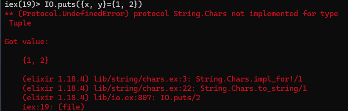
IO.puts({x, y} = {1, 2})
I got an undefined error
Formate para liderar los roles que están revolucionando el futuro del trabajo:
Falta agregar el área de Sostenibilidad y ESG
Reviewer #3 (Public review):
Summary:
The authors have studied the mechanics of bolalipid and archaeal mixed-lipid membranes via comprehensive molecular dynamics simulations. The Cooke-Deserno 3-bead-per-lipid model is extended to bolalipids with 6 bead. Phase diagrams, bending rigidity, mechanical stability of curved membranes, and cargo uptake are studied. Effects such as formation of U-shaped bolalipids, pore formation in highly curved regions, and changes in membrane rigidity are studied and discussed. The main aim has been to show how the mixture of bolalipids and regular bilayer lipids in archaeal membrane models enhances the fluidity and stability of these membranes.
The authors have presented a wide range of simulation results for different membrane conditions and conformations. Analyses and findings are presented clearly and concisely. Figures, supplementary information and movies are of very high quality and very well present what has been studied. The manuscript is well written and is easy to follow.
The authors have provided detailed response to the points I raised on the first version and have revised their manuscript accordingly. Hence, I only mention what, in my opinion, still deserves to be noted.
Comments:
I previously raised an issue with respect to the resort to the Hamm-Kozlov model for fitting the power spectrum of membrane undulations. The authors provided very nice arguments against my concerns. For the sake of completeness, I include a simple scenario, which will better highlight the issue:
The tilt contribution to the Helfrich Hamiltonian can be written as a quadratic term 1/2 k_t |T|^2, where T is a tilt vector field. This field is written as the difference between the surface normal and the director field aligned with the lipid orientations. In the small deviation Monge description with z=h(x, y) as the height function, the surface normal has the form N=(-dh/dx, -dh/dy, 1). Now assume the director field, n = (b_x, b_y, 1) with small b_x and b_y components. The tilt contribution to the energy thus reads as 1/2 k_t (N - n)^2 ~= 1/2 k_t [|grad h|^2 + 2 b . grad h]. The first term, 1/2 k_t |grad h|^2, is indeed similar to a surface tension term, \sigma |grad h|^2 that you get from the (1 + 1/2 |grad h|^2) approximation to the area element. Therefore, if you only look at height fluctuations, while your membrane actually has some surface tension, it will make distinguishing the tilt contributions to the fluctuations in the linear Monge gauge impossible.
However, considering that the authors have made sure that the membrane is indeed tensionless, this argument is settled.
I had also raised an issue about the correct NpT sampling in the simulations, and I'm glad that the authors also set up more rigorously thermostatted/barostatted simulations to check the validity of their findings.
Also, from the SI, I previously noted that the authors had neglected the longest wavelength mode because it was not equilibrated. This was an important problem and the authors looked into it and ran more simulations that were better equilibrated.
The analysis of energy of U-shaped lipids with the linear model E=c_0 + c_1 * k_bola is indeed very interesting. I am glad that the authors have expanded this analysis and included mean energy measurements.
Why, for example, does terrestrial life use only 20 of the scores of amino acids that can be produced
En este párrafo me llamó la atención esta pregunta y decidí indagar un poco. Según lo que investigué, pudo haber sido un proceso aleatorio, sin embargo, estos 20 aminoácidos fueron los que proporcionaron una base más solida para la vida, ya que, el código genético que traduce los genes en proteínas está limitados a estos 20 aminoácidos y habría tenido mayor dificultad si se hubieran incluido más; trayendo mutaciones fatales para la vida.
n 2021, the Hayabusa2 space mission successfully delivered a morsel of the asteroid 162173 Ryugu to Earth — five grams of the oldest, most pristine matter left over from the solar system’s formation 4.5 billion years ago. Last spring, scientists revealed that the chemical composition of the asteroid includes 10 amino acids, the building blocks of proteins. The discovery added to the evidence that the primordial soup from which life on Earth arose may have been seasoned with amino acids from pieces of asteroids.
esta investigación es que nos recuerda que la vida en la Tierra quizá no empezó únicamente aquí, sino que fue el resultado de una colaboración cósmica. Los rayos gamma, que normalmente asociamos con radiación peligrosa, en realidad pudieron ser la chispa que transformó simples moléculas en aminoácidos dentro de los asteroides. Es como si el universo mismo hubiera hecho una especie de laboratorio natural, preparando los ingredientes de la vida y enviándolos a nuestro planeta en forma de meteoritos.
El objetivo de este estudio fue describir las características pedagógicas en losprocesos evaluativos implementados en asignaturas virtuales en las Carreras deGrado en la Universidad Nacional de Villarrica del Espíritu Santo. Se analizaronen profundidad factores que caracterizan a una evaluación en un ambiente virtual,estrategias didácticas evaluativas, gestión de la evaluación y el seguimiento delestudiante. Se realizó un estudio de caso múltiple con enfoque mixto. Se observólas características evaluativas en las carreras de Licenciatura en Ciencias de laEducación e Ingeniería en Sistemas Informáticos. Los resultados muestran quelas evaluaciones implementadas son innovadoras y variadas, pero se identificaronalgunas limitaciones en cuanto a la claridad de los criterios de evaluación y lafrecuencia de retroalimentación individualizada. Estos hallazgos sugieren lanecesidad de fortalecer la formación docente en el diseño e implementación delas evaluaciones en ambientes virtuales
Necesito que realicen un resumen del siguiente texto
existen programas de posgrado (maestrías y doctorados) que aborden las humanidades digitales.
No existían para 2017, ya en 2025 hay algunas como es el caso de la que se imparte en la UAQuerétaro y en el Tec de Monterrey.
dweb.link@ http://bafybeihda4gloeygr5moflptlfedkbhkuysutw7ulbomreqfx6fywro4xa.ipfs.localhost:8080/?filename=%EF%BC%82display%20metaphor%20scripting%20language%EF%BC%82%20gyuri%20lajos%20dime%20-%20Brave%20Search%20(8_12_2025%209%EF%BC%9A35%EF%BC%9A01%20AM).html
for = wikify myself
CSP vs Actor model for concurrency -

Discussion on: CSP vs Actor model for concurrency
my comment on this
BDSC:59958
DOI: 10.1093/genetics/iyaf151
Resource: RRID:BDSC_59958
Curator: @scibot
SciCrunch record: RRID:BDSC_59958
Aunque los biocombustibles suelen considerarse una opción ecológica, su producción a partir de cultivos agrícolas provoca más daños que beneficios: favorece la deforestación, incrementa las emisiones de CO₂ de manera indirecta, encarece los alimentos y amenaza a los ecosistemas. Solo tendrían un verdadero valor sustentable si se elaboran con residuos o mediante tecnologías que no compitan con la agricultura ni demanden grandes extensiones de tierra.
Communication
Est-ce qu'il y a moyen que le bas du tableau soit enligné avec ceux de gauche? (voir les flèches ou venir me voir si mon commentaire n'est pas claire)
Formation financière
Est-ce qu'il y a moyen que le bas du tableau soit enligné avec ceux de gauche et droite? (voir les flèches ou venir me voir si mon commentaire n'est pas claire)
Financial Training
Est-ce qu'il y a moyen que le bas du tableau soit enligné avec ceux de gauche et droite? (voir les flèches ou venir me voir si mon commentaire n'est pas claire)
y 1 sc * v 1 ; P{TRiP.HMC05965}attP40
DOI: 10.1083/jcb.201709026
Resource: RRID:BDSC_65150
Curator: @maulamb
SciCrunch record: RRID:BDSC_65150
Reproducible analysis
Me da la impresión que este debiera ser el objetivo fuerte a impulsar dentro del ecosistema de la ciencia abierta. Digo, sobre el que más trabajo falta por hacer. Se podrían citar los ejercicios de replicación de Breznau. No necesariamente acá, sino más adelante al momento de habalr sobre el caso de Chile y latinoamérica.
However, like many others developments in science, the open science movementhas arrived slowly to Latin America, especially in social sciences. Although there have been some initiativesin recent years, most of them are driven mainly by the natural sciences.
Acá sería bueno señalar que en términos generales, la mayoría de los logros en ciencias sociales en América Latina se concentran en el crecimiento de fuentes y publicaciones abiertas como Scielo o Redalyc: https://www.ouvrirlascience.fr/latin-america-could-become-a-world-leader-in-non-commercial-open-science/
Author response:
The following is the authors’ response to the original reviews.
Reviewer #1 (Public review):
Summary:
In this study by Li et al., the authors re-investigated the role of cDC1 for atherosclerosis progression using the ApoE model. First, the authors confirmed the accumulation of cDC1 in atherosclerotic lesions in mice and humans. Then, in order to examine the functional relevance of this cell type, the authors developed a new mouse model to selectively target cDC1. Specifically, they inserted the Cre recombinase directly after the start codon of the endogenous XCR1 gene, thereby avoiding off-target activity. Following validation of this model, the authors crossed it with ApoE-deficient mice and found a striking reduction of aortic lesions (numbers and size) following a high-fat diet. The authors further characterized the impact of cDC1 depletion on lesional T cells and their activation state. Also, they provide in-depth transcriptomic analyses of lesional in comparison to splenic and nodal cDC1. These results imply cellular interactions between lesion T cells and cDC1. Finally, the authors show that the chemokine XCL1, which is produced by activated CD8 T cells (and NK cells), plays a key role in the interaction with XCR1-expressing cDC1 and particularly in the atherosclerotic disease progression.<br /> Strengths:
The surprising results on XCL1 represent a very important gain in knowledge. The role of cDC1 is clarified with a new genetic mouse model.
Thank you
Weaknesses:
My criticism is limited to the analysis of the scRNAseq data of the cDC1. I think it would be important to match these data with published data sets on cDC1. In particular, the data set by Sophie Janssen's group on splenic cDC1 might be helpful here (PMID: 37172103; https://www.single-cell.be/spleen_cDC_homeostatic_maturation/datasets/cdc1). It would be good to assign a cluster based on the categories used there (early/late, immature/mature, at least for splenic DC).
Thank you very much for your help. Using the scRNA seq data of Xcr1<sup>+</sup> cDC1 sorted from ApoE<sup>–/–</sup> mice, we re-annotated the populations, following the methodology proposed by Sophie Janssen's group. These results are presented in Figure S9 and Figure S10 and described in detail in the Results and Discussion section.
Please refer to the Results section from line 264 to 284: “Using the scRNA seq data of Xcr1<sup>+</sup> cDC1 sorted from hyperlipidemic mice, we annotated the 10 populations as shown in Figure S9A, following the methodology from a previous study [41]. Ccr7<sup>+</sup> mature cDC1s (Cluster 3, 7 and 9) and Ccr7- immature cDC1s (remaining clusters) were identified across cDC1 cells sorted from aorta, spleen and lymph nodes (Figure S9B). Further stratification based on marker genes reveals that Cluster 10 is the pre-cDC1, with high expression level of CD62L (Sell) and low expression level of CD8a (Figure S9C). Cluster 6 and 8 are the proliferating cDC1s, which express high level of cell cycling genes Stmn1 and Top2a (Figure S9D). Cluster 1 and 4 are early immature cDC1s, and cluster 2 and 5 are late immature cDC1s, according to the expression pattern of Itgae, Nr4a2 (Figure S9E). Cluster 9 cells are early mature cDC1s, with elevated expression of Cxcl9 and Cxcl10 (Figure S9F). Cluster 3 and 7 as late mature cDC1s, characterized by the expression of Cd63 and Fscn1 (Figure S9G). As shown in Figure 5C and Figure S9, the 10 populations displayed a major difference of aortic cDC1 cells that lack in pre-cDC1s (cluster 10) and mature cells (cluster 3, 7 and 9). Interestingly, in hyperlipidemic mice splenic cDC1 possess only Cluster 3 as the late mature cells while the lymph node cDC1 cells have two late mature populations namely Cluster 3 and Cluster 7. In further analysis, we also compared splenic cDC1 cells from HFD mice to those from ND mice. As shown in Figure S10, HFD appears to impact early immature cDC1-1 cells (Cluster 1) and increases the abundance of late immature cDC1 cells (Cluster 2 and 5), regardless of the fact that all 10 populations are present in two origins of samples. We also found that Tnfaip3 and Serinc3 are among the most upregulated genes, while Apol7c and Tifab are downregulated in splenic cDC1 cells sorted from HFD mice”.
Please refer to the Discussion section from line 380 to 385: “Based on the maturation analysis of the cDC1 scRNA seq data [41], our findings suggest that the aortic cDC1 cells display a major difference from those of spleen and lymph nodes by lacking the mature clusters, whereas lymph node cDC1 cells contain an additional Fabp5<sup>+</sup> S100a4<sup>+</sup> late mature Cluster. Our results also suggest that hyperlipidemia contributes to alteration in early immature cDC1 and in the abundance of late immature cDC1 cells, which was associated with dramatic change in gene expression of Tnfaip3, Serinc3, Apol7c and Tifab”.
Reviewer #2 (Public review):
This study investigates the role of cDC1 in atherosclerosis progression using Xcr1Cre-Gfp Rosa26LSL-DTA ApoE-/- mice. The authors demonstrate that selective depletion of cDC1 reduces atherosclerotic lesions in hyperlipidemic mice. While cDC1 depletion did not alter macrophage populations, it suppressed T cell activation (both CD4+ and CD8+ subsets) within aortic plaques. Further, targeting the chemokine Xcl1 (ligand of Xcr1) effectively inhibits atherosclerosis. The manuscript is well-written, and the data are clearly presented. However, several points require clarification:
(1) In Figure 1C (upper plot), it is not clear what the Xcr1 single-positive region in the aortic root represents, or whether this is caused by unspecific staining. So I wonder whether Xcr1 single-positive staining can reliably represent cDC1. For accurate cDC1 gating in Figure 1E, Xcr1+CD11c+ co-staining should be used instead.
The observed false-positive signal in the wavy structures within immunofluorescence Figure 1C (upper panel) results from the strong autofluorescence of elastic fibers, a major vascular wall component (alongside collagen). This intrinsic property of elastic fibers is a well-documented confounder in immunofluorescence studies [A, B].
In contrast, immunohistochemistry (IHC) employs an enzymatic chromogenic reaction (HRP with DAB substrate) that generates a brown precipitate exclusively at antigen-antibody binding sites. Importantly, vascular elastic fibers lack endogenous enzymatic activity capable of catalyzing the DAB reaction, thereby preventing this source of false positivity in IHC.
Given that Xcr1 is exclusively expressed on conventional type 1 dendritic cells [C], and considering that IHC lacks the multiplexing capability inherent to immunofluorescence for antigen co-localization, single-positive Xcr1 staining reliably identifies cDC1s in IHC results.
[A] König, K et al. “Multiphoton autofluorescence imaging of intratissue elastic fibers.” Biomaterials vol. 26,5 (2005): 495-500. doi:10.1016/j.biomaterials.2004.02.059
[B] Andreasson, Anne-Christine et al. “Confocal scanning laser microscopy measurements of atherosclerotic lesions in mice aorta. A fast evaluation method for volume determinations.” Atherosclerosis vol. 179,1 (2005): 35-42. doi:10.1016/j.atherosclerosis.2004.10.040
[C] Dorner, Brigitte G et al. “Selective expression of the chemokine receptor XCR1 on cross-presenting dendritic cells determines cooperation with CD8+ T cells.” Immunity vol. 31,5 (2009): 823-33. doi:10.1016/j.immuni.2009.08.027
(2) Figure 4D suggests that cDC1 depletion does not affect CD4+/CD8+ T cells. However, only the proportion of these subsets within total T cells is shown. To fully interpret effects, the authors should provide:
(a) Absolute numbers of total T cells in aortas.
(b) Absolute counts of CD4+ and CD8+ T cells.
Thanks for your suggestions. We agree that assessing both proportions and absolute numbers in Figure 4 provides a more complete picture of the effects of cDC1 depletion on T cell populations. Furthermore, we also add the absolute count of cDC1 cells and total T cells, and CD44 MFI (mean fluorescence intensity) in CD4<sup>+</sup> and CD8<sup>+</sup> T cells in Figure 4, and supplemented corresponding textual descriptions in the revised manuscript.
Please refer to the Results section from line 183 to 187: “Subsequently, we assessed T cell phenotype in the two groups of mice. While neither the frequencies nor absolute counts of aortic CD4<sup>+</sup> and CD8<sup>+</sup> T cells differed significantly between two groups of mice (Figure 4D-F), CD69 frequency and CD44 MFI (Mean Fluorescence Intensity), the T cell activation markers, were significantly reduced in both CD4<sup>+</sup> and CD8<sup>+</sup> T cells from Xcr1<sup>+</sup> cDC1 depleted mice compared to controls (Figure 4G and H)”.
(3) How does T cell activation mechanistically influence atherosclerosis progression? Why was CD69 selected as the sole activation marker? Were other markers (e.g., KLRG1, ICOS, CD44) examined to confirm activation status?
We sincerely appreciate these insightful comments. As extensively documented in the literature, activated effector T cells (both CD4+ and CD8+) critically promote plaque inflammation and instability through their production of pro-inflammatory cytokines (particularly IFN-γ and TNF-α), which drive endothelial activation, exacerbate macrophage inflammatory responses, and impair smooth muscle cell function [A].
In our study, we specifically investigated the role of cDC1 cells in atherosclerosis progression. Our key findings demonstrate that cDC1 depletion attenuates T cell activation (as shown by reduced CD69/CD44 expression) and that this reduction in activation is functionally linked to the observed decrease in atherosclerosis burden in our model.
Regarding CD44 as an activation marker, we performed quantitative analyses of CD44 mean fluorescence intensity (MFI) in aortic T cells (Figure 4). Importantly, the MFI of CD44 was significantly lower on both CD4+ and CD8+ T cells from Xcr1<sup>Cre-Gfp</sup> Rosa26<sup>LSL-DTA</sup> ApoE<sup>–/–</sup> mice compared to the control ApoE<sup>–/–</sup> mice (data shown below), which is consistent with the result of CD69 in Figure 4. We added the related description in the Result section.
Please refer to the Results section from line 185 to 187 “CD69 frequency and CD44 MFI (Mean Fluorescence Intensity), the T cell activation markers, were significantly reduced in both CD4+ and CD8+ T cells from Xcr1+ cDC1 depleted mice compared to controls (Figure 4G and H)”.
Similarly, MFI of CD44 was significantly lower on both CD4<sup>+</sup> and CD8<sup>+</sup> T cells from Xcl1<sup>–/–</sup> ApoE<sup>–/–</sup> mice compared to the control ApoE<sup>–/–</sup> mice (data shown below), which is consistent with the result of CD69 in Figure 7. We also added the related description in the Result section.
Please refer to the Results section from line 308 to 309 “Crucially, CD69<sup>+</sup> frequency and CD44 MFI remained comparable in both aortic CD4<sup>+</sup> and CD8<sup>+</sup> T cells between two groups (Figure 7D-F).”
[A] Hansson, Göran K, and Andreas Hermansson. “The immune system in atherosclerosis.” Nature immunology vol. 12,3 (2011): 204-12. doi:10.1038/ni.2001
(4) Figure 7B: Beyond cDC1/2 proportions within cDCs, please report absolute counts of: Total cDCs, cDC1, and cDC2 subsets. Figure 7D: In addition to CD4+/CD8+ T cell proportions, the following should be included:
(a) Total T cell numbers in aortas
(b) Absolute counts of CD4+ and CD8+ T cells.
Thanks for your suggestions. We have now included in Figure 7 the absolute counts of cDC, cDC1, and cDC2 cells, along with CD4<sup>+</sup> and CD8<sup>+</sup> T cells in aortic tissues. Additionally, we provide the corresponding CD44 mean fluorescence intensity (MFI) measurements for both CD4<sup>+</sup> and CD8<sup>+</sup> T cell populations. We added the related description in the Result section.
Please refer to the Results section from line 303 to 311: “The flow cytometric results illustrated that both frequencies and absolute counts of Xcr1<sup>+</sup> cDC1 cells in the aorta were significantly reduced, but cDCs and cDC2 cells from Xcl1<sup>–/–</sup> ApoE<sup>–/–</sup> were comparable with that from ApoE<sup>–/–</sup> (Figure 7A-C). Moreover, in both lymph node and spleen, the absolute numbers of pDC, cDC1 and cDC2 from Xcl1<sup>–/–</sup> ApoE<sup>–/–</sup> were comparable with that from ApoE<sup>–/–</sup> (Figure S11). Crucially, CD69<sup>+</sup> frequency and CD44 MFI remained comparable in both aortic CD4<sup>+</sup> and CD8<sup>+</sup> T cells between two groups (Figure 7D-F). However, aortic CD8<sup>+</sup> T cells exhibited reduced frequency and absolute count, while CD4<sup>+</sup> T cells showed increased frequency but unchanged counts in Xcl1<sup>–/–</sup> ApoE<sup>–/–</sup> mouse versus controls (Figure 7G and H).”
(5) cDC1 depletion reduced CD69+CD4+ and CD69+CD8+ T cells, whereas Xcl1 depletion decreased Xcr1+ cDC1 cells without altering activated T cells. How do the authors explain these different results? This discrepancy needs explanation.
We sincerely appreciate your professional and insightful comments regarding the mechanistic relationship between cDC1 depletion and T cell activation. Direct cDC1 depletion in the Xcr1<sup>Cre-Gfp</sup> Rosa26<sup>LSL-DTA</sup> ApoE<sup>–/–</sup> micmodel removes both recruited and tissue-resident cDC1s, eliminating their multifunctional roles in antigen presentation, co-stimulation and cytokine secretion essential for T cell activation. In contrast, Xcl1 depletion reduces, but does not eliminate cDC1 migration into plaques. Furthermore, alternative chemokine axes (e.g., CCL5/CCR5, CXCL9/CXCR3, BCL9/BCL9L) may partially rescue cDC1 recruitment [13, 68, 69], and non-cDC1 APCs (e.g., monocytes, cDC2s) may compensate for T cell activation [55, 70]. We emphasize that Xcl1 depletion specifically failed to alter T cell activation in hyperlipidemic ApoE<sup>–/–</sup> mice. However, its impact may differ in other pathophysiological contexts due to compensatory mechanisms. We thank you again for highlighting this nuance, which strengthens our mechanistic interpretation. We have added these points to the discussion section and included new references.
Please refer to the Discussion section from line 407 to 413: “Notably, while complete ablation of Xcr1<sup>+</sup> cDC1s impaired T cell activation, reduction of Xcr1<sup>+</sup> cDC1 recruitment via Xcl1 deletion did not significantly compromise this process. This discrepancy may arise through compensatory mechanisms: alternative chemokine axes (e.g., CCL5/CCR5, CXCL9/CXCR3, BCL9/BCL9L) may partially rescue Xcr1<sup>+</sup> cDC1 homing [13, 68, 69], while non-cDC1 antigen-presenting cells (e.g., monocytes, cDC2s) may sustain T cell activation [55, 70]. Furthermore, tissue-specific microenvironment factors could potentially modulate its role in other diseases.”. [13] Eisenbarth, S C. “Dendritic cell subsets in T cell programming: location dictates function.” Nature reviews. Immunology vol. 19,2 (2019): 89-103. doi:10.1038/s41577-018-0088-1 [55] Brewitz, Anna et al. “CD8+ T Cells Orchestrate pDC-XCR1+ Dendritic Cell Spatial and Functional Cooperativity to Optimize Priming.” Immunity vol. 46,2 (2017): 205-219. doi:10.1016/j.immuni.2017.01.003 [68] de Oliveira, Carine Ervolino et al. “CCR5-Dependent Homing of T Regulatory Cells to the Tumor Microenvironment Contributes to Skin Squamous Cell Carcinoma Development.” Molecular cancer therapeutics vol. 16,12 (2017): 2871-2880. doi:10.1158/1535-7163.MCT-17-0341.[69] He F, Wu Z, Liu C, Zhu Y, Zhou Y, Tian E, et al. Targeting BCL9/BCL9L enhances antigen presentation by promoting conventional type 1 dendritic cell (cDC1) activation and tumor infiltration. Signal Transduct Target Ther. 2024;9(1):139. Epub 2024/05/30. doi: 10.1038/s41392-024-01838-9. PubMed PMID: 38811552; PubMed Central PMCID: PMCPMC11137111.[70] Böttcher, Jan P et al. “Functional classification of memory CD8(+) T cells by CX3CR1 expression.” Nature communications vol. 6 8306. 25 Sep. 2015, doi:10.1038/ncomms9306.
Reviewer #1 (Recommendations for the authors):
(1) Line 32 - The authors might want to add that the mouse model leads to a "constitutive" depletion of cDC1.
Thanks for your advice, we have revised the sentence as follows.
Please refer to the Results section from line 31 to 33: “we established Xcr1<sup>Cre-Gfp</sup> Rosa26<sup>LSL-DTA</sup> ApoE<sup>–/–</sup> mice, a novel and complex genetic model, in which cDC1 was constitutively depleted in vivo during atherosclerosis development”.
(2) Line 187-188: The authors claim that T cell activation was "inhibited" if cDC1 was depleted. The data shows that the T cells were less activated, but there is no indication of any kind of inhibition; this should be corrected.
Thanks for your advice, we have revised the sentence as follows.
Please refer to the Results section from line 183 to 187: “Subsequently, we assessed T cell phenotype in the two groups of mice. While neither the frequencies nor absolute counts of aortic CD4<sup>+</sup> and CD8<sup>+</sup> T cells differed significantly between two groups of mice (Figure 4D-F), CD69 frequency and CD44 MFI (Mean Fluorescence Intensity), the T cell activation markers, were significantly reduced in both CD4<sup>+</sup> and CD8<sup>+</sup> T cells from Xcr1<sup>+</sup> cDC1 depleted mice compared to controls (Figure 4G and H)”.
(3) Why are some splenic DC clusters absent in LNs and vice versa? This is not obvious to this reviewer and should at least be discussed.
We appreciate the insightful question regarding the absence of certain splenic DC clusters in LNs. This phenomenon in Figure 5 aligns with the 'division of labor' paradigm in dendritic cell biology: tissue microenvironments evolve specialized DC subsets to address local immunological challenges. The absence of universal clusters reflects functional adaptation, not technical artifacts. We acknowledge that this tissue-specific heterogeneity warrants further discussion and have expanded our analysis to address this point in the discussion part of our manuscript.
Please refer to the Discussion section from line 375 to 385: “This pronounced tissue-specific compartmentalization of Xcr1<sup>+</sup> cDC1 subsets may related to multiple mechanisms including developmental imprinting that instructs precursor differentiation into transcriptionally distinct subpopulations [62], and microenvironmental filtering through organ-specific chemokine axes (e.g., CCL2/CCR2 in spleen) selectively recruits receptor-matched subsets [63, 64]. This spatial specialization optimizes pathogen surveillance for local immunological challenges. Based on the maturation analysis of the cDC1 scRNA seq data [41], our findings suggest that the aortic cDC1 cells display a major difference from those of spleen and lymph nodes by lacking the mature clusters, whereas lymph node cDC1 cells contain an additional Fabp5<sup>+</sup> S100a4<sup>+</sup> late mature Cluster. Our results also suggest that hyperlipidemia contributes to alteration in early immature cDC1 and in the abundance of late immature cDC1 cells, which was associated with dramatic change in gene expression of Tnfaip3, Serinc3, Apol7c and Tifab”.
[62]. Liu Z, Gu Y, Chakarov S, Bleriot C, Kwok I, Chen X, et al. Fate Mapping via Ms4a3-Expression History Traces Monocyte-Derived Cells. Cell. 2019;178(6):1509-25 e19. Epub 2019/09/07. doi: 10.1016/j.cell.2019.08.009. PubMed PMID: 31491389.
[63]. Bosmans LA, van Tiel CM, Aarts S, Willemsen L, Baardman J, van Os BW, et al. Myeloid CD40 deficiency reduces atherosclerosis by impairing macrophages' transition into a pro-inflammatory state. Cardiovasc Res. 2023;119(5):1146-60. Epub 2022/05/20. doi: 10.1093/cvr/cvac084. PubMed PMID: 35587037; PubMed Central PMCID: PMCPMC10202633.
[64]. Mildner A, Schonheit J, Giladi A, David E, Lara-Astiaso D, Lorenzo-Vivas E, et al. Genomic Characterization of Murine Monocytes Reveals C/EBPbeta Transcription Factor Dependence of Ly6C(-) Cells. Immunity. 2017;46(5):849-62 e7. Epub 2017/05/18. doi: 10.1016/j.immuni.2017.04.018. PubMed PMID: 28514690.
[41]. Bosteels V, Marechal S, De Nolf C, Rennen S, Maelfait J, Tavernier SJ, et al. LXR signaling controls homeostatic dendritic cell maturation. Sci Immunol. 2023;8(83):eadd3955. Epub 2023/05/12. doi: 10.1126/sciimmunol.add3955. PubMed PMID: 37172103.
(4) The authors should discuss how XCL1 could impact lesional cDC1 and T cell abundance. Notably, preDCs do not express XCR1, and T cells express XCL1 following TCR activation. Is there a recruitment or local proliferation defect of cDC1 in the absence of XCL1? Could there also be a role for NK cells as a potential source of XCL1?
We appreciate your insightful questions regarding the differential effects of Xcl1 on cDC1s and T cells. Xcl1 primarily mediates the recruitment of mature cDC1s. Our data demonstrate that Xcl1 deletion significantly reduces aortic cDC1 abundance, which correlates with a concomitant decrease in CD8<sup>+</sup> T cell numbers within the aorta. These findings strongly suggest that the Xcl1-Xcr1 axis plays a regulatory role in T cell accumulation in aortic plaques.
Consistent with prior studies [A, B], cDC1 recruitment can occur in the absence of Xcl1 which echoes our findings that cDC1 cells were still found in Xcl1 knockout aortic plaque but in lower abundance. It is very true that further studies are required to address how the Xcl1 dependent and independent cDC1 cells activate T cells and if they possess capability of proliferation in tissue differentially. We have added these points in discussion section.
Please refer to the Discussion section from line 407 to 415: “Notably, while complete ablation of Xcr1<sup>+</sup> cDC1s impaired T cell activation, reduction of Xcr1<sup>+</sup> cDC1 recruitment via Xcl1 deletion did not significantly compromise this process. This discrepancy may arise through compensatory mechanisms: alternative chemokine axes (e.g., CCL5/CCR5, CXCL9/CXCR3, BCL9/BCL9L) may partially rescue Xcr1<sup>+</sup> cDC1 homing [13, 68, 69], while non-cDC1 antigen-presenting cells (e.g., monocytes, cDC2s) may sustain T cell activation [55, 70]. Furthermore, tissue-specific microenvironment factors could potentially modulate its role in other diseases. In summary, our findings identify Xcl1 as a potential therapeutic target for atherosclerosis therapy, though its cellular origins and regulation of lesional Xcr1<sup>+</sup> cDC1 and T cells dynamics require further studies”.
In literatures, Xcl1 are expressed in NK cells and subsects of T cells, and NK cells can be a potential source of Xcl1 during atherosclerosis which deserve further investigations [A, C, D].
[A] Böttcher, Jan P et al. “NK Cells Stimulate Recruitment of cDC1 into the Tumor Microenvironment Promoting Cancer Immune Control.” Cell vol. 172,5 (2018): 1022-1037.e14. doi:10.1016/j.cell.2018.01.004
[B] He, Fenglian et al. “Targeting BCL9/BCL9L enhances antigen presentation by promoting conventional type 1 dendritic cell (cDC1) activation and tumor infiltration.” Signal transduction and targeted therapy vol. 9,1 139. 29 May. 2024, doi:10.1038/s41392-024-01838-9
[C] Woo, Yeon Duk et al. “The invariant natural killer T cell-mediated chemokine X-C motif chemokine ligand 1-X-C motif chemokine receptor 1 axis promotes allergic airway hyperresponsiveness by recruiting CD103+ dendritic cells.” The Journal of allergy and clinical immunology vol. 142,6 (2018): 1781-1792.e12. doi:10.1016/j.jaci.2017.12.1005
[D] Winkels, Holger et al. “Atlas of the Immune Cell Repertoire in Mouse Atherosclerosis Defined by Single-Cell RNA-Sequencing and Mass Cytometry.” Circulation research vol. 122,12 (2018): 1675-1688. doi:10.1161/CIRCRESAHA.117.312513
Reviewer #2 (Recommendations for the authors):
There is a logical error in line 298. I suggest revising to: "Collectively, these data suggest that Xcl1 promotes atherosclerosis by recruiting Xcr1+ cDC1 cells, which subsequently drive T cell activation in lesions."
Thanks for your advice. Since Xcl1 deficiency reduced both the frequencies and absolute counts of Xcr1+ cDC1 and CD8+ T cells in lesions without affecting T cell activation, we revised the sentence as you suggested.
Please refer to the Results section from line 314 to 315: “Collectively, these data suggest that Xcl1 promotes atherosclerosis by recruiting Xcr1<sup>+</sup> cDC1 cells, and facilitating CD8<sup>+</sup> T cell accumulation in lesions”.
Propuesta ELSOC
partir con propuesta América Latina ... y dar contexto
.
seguido a esto: a partir de este marco conceptual, el OCS ... (dar contexto a lo que sigue)
Y no se dice nada sobre que de aquí en adelante estamos solo hablando de cohesión horizontal
Este esquema de medición se compone por tres dimensiones de segundo orden: Sentido de pertenencia (1), el cual se compone por un dos indicadores; uno de identidad nacional y orgullo por el país. Calidad de la vida en el vecindario (2), construida mediante cuatro factores, en donde el único que contiene un indicador es el de confianza en vecinos. Y por último Redes sociales (3), que contiene un factor de confianza interpersonal y otro de comportamiento prosocial.
no será mejor agregar en el mismo esquema cuáles son dimensiones y cuáles subdimensiones?
El Centro de Estudios de Conflicto y Cohesión Social es una iniciativa que surge el año 2014 con la intención de estudiar desde una perspectiva multidimensional los factores que agudizan el conflicto social y aquellos que fortalecen la cohesión social en Chile. A través del trabajo investigativo, la colaboración con instituciones públicas y la formación de capital humano avanzado, COES se presenta como un centro que busca el vínculo entre ciencia, Estado y sociedad, proponiendo diagnósticos y soluciones que contribuyan al desarrollo y bienestar del país.
párrafo 2 de introducción, y falta agregar lo del OCS
El primer trabajo mencionado es uno de los antecedentes principales del actual trabajo, puesto que, a partir de una revisión sistemática de estudios internacionales, busca identificar los principales indicadores que posibilitan la operacionalización y medición de la cohesión social en Chile con los datos de ELSOC. El segundo documento pretende aportar en la medición de la cohesión social pero a un nivel regional, abordando la construcción técnica y metodológica para medir este fenómeno en América Latina.
mejor incluir la descripción en párrafo arriba
RRID:SCR_002798
DOI: 10.1038/s41386-025-02142-y
Resource: GraphPad Prism (RRID:SCR_002798)
Curator: @scibot
SciCrunch record: RRID:SCR_002798
Reviewer #2 (Public Review):
Summary:
This paper describes a new approach to detecting directed causal interactions between two genes without directly perturbing either gene. To check whether gene X influences gene Z, a reporter gene (Y) is engineered into the cell in such a way that (1) Y is under the same transcriptional control as X, and (2) Y does not influence Z. Then, under the null hypothesis that X does not affect Z, the authors derive an equation that describes the relationship between the covariance of X and Z and the covariance of Y and Z. Violation of this relationship can then be used to detect causality.
The authors benchmark their approach experimentally in several synthetic circuits. In 4 positive control circuits, X is a TetR-YFP fusion protein that represses Z, which is an RFP reporter. The proposed approach detected the repression interaction in 2 of the 4 positive control circuits. The authors constructed 16 negative control circuit designs in which X was again TetR-YFP, but where Z was either a constitutively expressed reporter, or simply the cellular growth rate. The proposed method detected a causal effect in two of the 16 negative controls, which the authors argue is perhaps not a false positive, but due to an unexpected causal effect. Overall, the data support the potential value of the proposed approach.
Strengths:
The idea of a "no-causality control" in the context of detected directed gene interactions is a valuable conceptual advance that could potentially see play in a variety of settings where perturbation-based causality detection experiments are made difficult by practical considerations.
By proving their mathematical result in the context of a continuous-time Markov chain, the authors use a more realistic model of the cell than, for instance, a set of deterministic ordinary differential equations.
The authors have improved the clarity and completeness of their proof compared to a previous version of the manuscript.
Limitations:
The authors themselves clearly outline the primary limitations of the study: The experimental benchmark is a proof of principle, and limited to synthetic circuits involving a handful of genes expressed on plasmids in E. coli. As acknowledged in the Discussion, negative controls were chosen based on the absence of known interactions, rather than perturbation experiments. Further work is needed to establish that this technique applies to other organisms and to biological networks involving a wider variety of genes and cellular functions. It seems to me that this paper's objective is not to delineate the technique's practical domain of validity, but rather to motivate this future work, and I think it succeeds in that.
Might your new "Proposed additional tests" subsection be better housed under Discussion rather than Results?
I may have missed this, but it doesn't look like you ran simulation benchmarks of your bootstrap-based test for checking whether the normalized covariances are equal. It would be useful to see in simulations how the true and false positive rates of that test vary with the usual suspects like sample size and noise strengths.
It looks like you estimated the uncertainty for eta_xz and eta_yz separately. Can you get the joint distribution? If you can do that, my intuition is you might be able to improve the power of the test (and maybe detect positive control #3?). For instance, if you can get your bootstraps for eta_xz and eta_yz together, could you just use a paired t-test to check for equality of means?
The proof is a lot better, and it's great that you nailed down the requirement on the decay of beta, but the proof is still confusing in some places:
On pg 29, it says "That is, dividing the right equation in Eq. 5.8 with alpha, we write the ..." but the next equation doesn't obviously have anything to do with Eq. 5.8, and instead (I think) it comes from Eq 5.5. This could be clarified.
Later on page 29, you write "We now evoke the requirement that the averages xt and yt are stationary", but then you just repeat Eq. 5.11 and set it to zero. Clearly you needed the limit condition to set Eq. 5.11 to zero, but it's not clear what you're using stationarity for. I mean, if you needed stationarity for 5.11 presumably you would have referenced it at that step.
It could be helpful for readers if you could spell out the practical implications of the theorem's assumptions (other than the no-causality requirement) by discussing examples of setups where it would or wouldn't hold.
Reviewer #4 (Public review):
Summary:
In this paper, Derkaloustian et al. look at the important topic of what affects fine touch perception. The observations that there may be some level of correlation with instabilities are intriguing. They attempted to characterize different materials by counting the frequency (occurrence #, not of vibration) of instabilities at various speeds and forces of a PDMS slab pulled lengthwise over the material. They then had humans perform the same vertical motion to discriminate between these samples. They correlated the % correct in discrimination with differences in frequency of steady sliding over the design space as well as other traditional parameters such as friction coefficient and roughness.
The authors pose an interesting hypothesis and make an interesting observation about the occurrences of instability regimes in different materials while in contact with PDMS, which is interesting for the community to see in publication. It should be noted however that the finger is complex, and there are many factors that may be over simplified, and perhaps even incorrect, with the use of the PDMS finger. There are trends, such as the trend of surfaces that are more similar in PDMS friction coefficient being easier to discriminate than those with more different PDMS friction coefficient, that contradict multiple other papers in the literature (Fehlberg et al., 2024; Smith and Scott, 1996). This may be due to the PDMS finger not being representative of the real finger conditions. A measurement of friction and the instabilities with a human finger, or demonstration that the PDMS finger is producing the same results (friction coefficient, instabilities, etc.) as a human finger, is needed.
Strengths:
The strength of this paper is in its intriguing hypothesis and important observation that instabilities may contribute to what humans are detecting as differences in these apparently similar samples.
Weaknesses:
There is are significant weaknesses in the representativeness of the PDMS finger, the vertical motion, and the speed of sliding to real human exploration. The real finger has multiple layers with different moduli. In fact, the stratum corneum cells, which are the outer layer at the interface and determine the friction, have much higher modulus than PDMS. In addition, the flat contact area can cause shifting of contact points. Both can contribute to making the PDMS finger have much more stick slip than a real finger. In fact, if you look at the regime maps, there is very little space that has steady sliding. This does not represent well human exploration of surfaces. We do not tend to use force and velocity that will cause extensive stick slip (frequent regions of 100% stick slip) and, in fact, the speeds used in the study are on the slow side, which also contributes to more stick slip. At higher speeds and lower forces, all of the materials had steady sliding regions. Further, on these very smooth surfaces, the friction and stiction are more complex and cannot dismiss considerations such as finger material property change with sweat pore occlusion and sweat capillary forces. Also, the vertical motion of both the PDMS finger and the instructed human subjects is not the motion that humans typically use to discriminate between surfaces.
This all leads to the critical question, why is the friction, normal force, and velocity not measured during the measured human exploration using the real human finger? An alternative would be showing that the PDMS finger reproduces the results of the human finger. I have checked the author's previous papers with this setup and did not find one that showed that the PDMS finger produced the same results as a human finger (Carpenter et al., 2018; Dhong et al., 2018; Nolin et al., 2022, 2021). The reviewer is not asking to do a more detailed psychophysical study with a decision-making model. All that is being asked is to use a human finger for the friction coefficient and instability measurements at typical human forces and speeds, or at least doing these measurements with both for one or two samples to show that the PDMS finger produces the same results as a human finger. The authors posed an extremely interesting hypothesis that humans may alter their speed to feel the instability transition regions. This is something that could be measured with a real finger but is not likely to be correlated accurately enough to match regime boundaries determined with such a simplified artificial finger.
References
Carpenter CW, Dhong C, Root NB, Rodriquez D, Abdo EE, Skelil K, Alkhadra MA, Ramírez J, Ramachandran VS, Lipomi DJ. 2018. Human ability to discriminate surface chemistry by touch. Mater Horiz 5:70-77. doi:10.1039/C7MH00800G<br /> Dhong C, Kayser LV, Arroyo R, Shin A, Finn M, Kleinschmidt AT, Lipomi DJ. 2018. Role of fingerprint-inspired relief structures in elastomeric slabs for detecting frictional differences arising from surface monolayers. Soft Matter 14:7483-7491. doi:10.1039/C8SM01233D<br /> Fehlberg M, Monfort E, Saikumar S, Drewing K, Bennewitz R. 2024. Perceptual Constancy in the Speed Dependence of Friction During Active Tactile Exploration. IEEE Transactions on Haptics 17:957-963. doi:10.1109/TOH.2024.3493421<br /> Nolin A, Licht A, Pierson K, Lo C-Y, Kayser LV, Dhong C. 2021. Predicting human touch sensitivity to single atom substitutions in surface monolayers for molecular control in tactile interfaces. Soft Matter 17:5050-5060. doi:10.1039/D1SM00451D<br /> Nolin A, Pierson K, Hlibok R, Lo C-Y, Kayser LV, Dhong C. 2022. Controlling fine touch sensations with polymer tacticity and crystallinity. Soft Matter 18:3928-3940. doi:10.1039/D2SM00264G<br /> Smith AM, Scott SH. 1996. Subjective scaling of smooth surface friction. Journal of Neurophysiology 75:1957-1962. doi:10.1152/jn.1996.75.5.1957
SD-Tg(GFP)Bal
DOI: 10.1038/s41598-017-10251-y
Resource: Rat Resource and Research Center (RRID:SCR_002044)
Curator: @Apiekniewska
SciCrunch record: RRID:SCR_002044
CRL-5935
DOI: 10.1038/s41586-025-09299-y
Resource: (ATCC Cat# CRL-5935, RRID:CVCL_1543)
Curator: @dhovakimyan1
SciCrunch record: RRID:CVCL_1543
CRL1424
DOI: 10.1038/s41586-025-09299-y
Resource: (TKG Cat# TKG 0197, RRID:CVCL_1220)
Curator: @dhovakimyan1
SciCrunch record: RRID:CVCL_1220
Addgene, 98290
DOI: 10.1038/s41586-025-09299-y
Resource: RRID:Addgene_98290
Curator: @dhovakimyan1
SciCrunch record: RRID:Addgene_98290
Addgene, 8454
DOI: 10.1038/s41586-025-09299-y
Resource: RRID:Addgene_8454
Curator: @dhovakimyan1
SciCrunch record: RRID:Addgene_8454
CRL-2868
DOI: 10.1038/s41586-025-09299-y
Resource: (KCLB Cat# 70827, RRID:CVCL_2063)
Curator: @dhovakimyan1
SciCrunch record: RRID:CVCL_2063
CCL-185
DOI: 10.1038/s41586-025-09299-y
Resource: (CCLV Cat# CCLV-RIE 1035, RRID:CVCL_0023)
Curator: @dhovakimyan1
SciCrunch record: RRID:CVCL_0023
Addgene, 8455
DOI: 10.1038/s41586-025-09299-y
Resource: RRID:Addgene_8455
Curator: @dhovakimyan1
SciCrunch record: RRID:Addgene_8455
CRL-5908
DOI: 10.1038/s41586-025-09299-y
Resource: (RRID:CVCL_1511)
Curator: @dhovakimyan1
SciCrunch record: RRID:CVCL_1511
CRL-5866
DOI: 10.1038/s41586-025-09299-y
Resource: (KCLB Cat# 91373, RRID:CVCL_1465)
Curator: @dhovakimyan1
SciCrunch record: RRID:CVCL_1465
CRL-3211
DOI: 10.1038/s41586-025-09299-y
Resource: (ICLC Cat# HTL97008, RRID:CVCL_1644)
Curator: @dhovakimyan1
SciCrunch record: RRID:CVCL_1644
CRL-2557
DOI: 10.1038/s41586-025-09299-y
Resource: (ATCC Cat# CRL-2557, RRID:CVCL_1637)
Curator: @dhovakimyan1
SciCrunch record: RRID:CVCL_1637
CRL-5924
DOI: 10.1038/s41586-025-09299-y
Resource: (ATCC Cat# CRL-5924, RRID:CVCL_1530)
Curator: @dhovakimyan1
SciCrunch record: RRID:CVCL_1530
CRL-5882
DOI: 10.1038/s41586-025-09299-y
Resource: (ATCC Cat# CRL-5882, RRID:CVCL_1482)
Curator: @dhovakimyan1
SciCrunch record: RRID:CVCL_1482
HTB-182
DOI: 10.1038/s41586-025-09299-y
Resource: (ATCC Cat# HTB-182, RRID:CVCL_1566)
Curator: @dhovakimyan1
SciCrunch record: RRID:CVCL_1566
CRL-5883
DOI: 10.1038/s41586-025-09299-y
Resource: (KCLB Cat# 91650, RRID:CVCL_1483)
Curator: @dhovakimyan1
SciCrunch record: RRID:CVCL_1483
CRL-6475
DOI: 10.1038/s41586-025-09299-y
Resource: (KCLB Cat# 80008, RRID:CVCL_0159)
Curator: @dhovakimyan1
SciCrunch record: RRID:CVCL_0159
CRL-2539
DOI: 10.1038/s41586-025-09299-y
Resource: (ATCC Cat# CRL-2539, RRID:CVCL_0125)
Curator: @dhovakimyan1
SciCrunch record: RRID:CVCL_0125
strain 005557
DOI: 10.1038/s41586-025-09299-y
Resource: (IMSR Cat# JAX_005557,RRID:IMSR_JAX:005557)
Curator: @dhovakimyan1
SciCrunch record: RRID:IMSR_JAX:005557
CRL-3216
DOI: 10.1038/s41586-025-09299-y
Resource: (RRID:CVCL_0063)
Curator: @dhovakimyan1
SciCrunch record: RRID:CVCL_0063
CRL-1469
DOI: 10.1038/s41586-025-09299-y
Resource: (ECACC Cat# 87092802, RRID:CVCL_0480)
Curator: @dhovakimyan1
SciCrunch record: RRID:CVCL_0480
CRL-1420
DOI: 10.1038/s41586-025-09299-y
Resource: (ATCC Cat# CRM-CRL-1420, RRID:CVCL_0428)
Curator: @dhovakimyan1
SciCrunch record: RRID:CVCL_0428
RRID:SCR_003070
DOI: 10.1038/s41586-025-09299-y
Resource: ImageJ (RRID:SCR_003070)
Curator: @scibot
SciCrunch record: RRID:SCR_003070
RRID:SCR_016366
DOI: 10.1038/s41586-025-09299-y
Resource: Deeptools (RRID:SCR_016366)
Curator: @scibot
SciCrunch record: RRID:SCR_016366
RRID:SCR_012919
DOI: 10.1038/s41586-025-09299-y
Resource: featureCounts (RRID:SCR_012919)
Curator: @scibot
SciCrunch record: RRID:SCR_012919
RRID:SCR_014583
DOI: 10.1038/s41586-025-09299-y
Resource: FastQC (RRID:SCR_014583)
Curator: @scibot
SciCrunch record: RRID:SCR_014583
RRID:SCR_013291
DOI: 10.1038/s41586-025-09299-y
Resource: MACS (RRID:SCR_013291)
Curator: @scibot
SciCrunch record: RRID:SCR_013291
RRID:SCR_016368
DOI: 10.1038/s41586-025-09299-y
Resource: Bowtie (RRID:SCR_005476)
Curator: @scibot
SciCrunch record: RRID:SCR_016368
RRID:SCR_011847
DOI: 10.1038/s41586-025-09299-y
Resource: Trim Galore (RRID:SCR_011847)
Curator: @scibot
SciCrunch record: RRID:SCR_011847
RRID:SCR_014228
DOI: 10.1038/s41586-025-09299-y
Resource: Sparky (RRID:SCR_014228)
Curator: @scibot
SciCrunch record: RRID:SCR_014228
TIB-207
DOI: 10.1007/s11307-025-02043-y
Resource: (IZSLER Cat# BS Hy 25, RRID:CVCL_4523)
Curator: @dhovakimyan1
SciCrunch record: RRID:CVCL_4523
RRID:AB_312686
DOI: 10.1007/s11307-025-02043-y
Resource: (BioLegend Cat# 100401, RRID:AB_312686)
Curator: @scibot
SciCrunch record: RRID:AB_312686
Les balises <em> et <strong> ne signifient pas respectivement “mettre en italique" ou "mettre en gras” mais seulement que le texte est “important”.
En fait, c'est comme s'il y avait des balises "imp 1", "imp 2" et "imp 3" et que le navigateur change de style selon le chiffre après le "imp", c'est ça ? Ce que je ne comprends pas, c'est que, si "strong" ne signifie pas, pour le navigateur, "mettre en gras", dans ce cas, il choisit aléatoirement entre "surligner", "italique" et "gras" ? Mais dans ce cas, pourquoi des balises spécifiques pour chacun des styles ?
Dirgelwch y Bedd Heb Gorff |<br /> by [[Jimmy Johnson]] for [[S4C]] accessed on 2025-08-13T00:11:28 Uncovering Secrets of a Pembrokeshire Cemetery | TheWelshViking | S4C - YouTube
gwylnos (night watch) - similar to an Irish wake
hirwen-gwd - tradition of wrapping a body in a white shroud and using a rope to raise and lower them in the chimney
Author response:
The following is the authors’ response to the original reviews
eLife Assessment
This valuable study revisits the effects of substitution model selection on phylogenetics by comparing reversible and non-reversible DNA substitution models. The authors provide evidence that 1) non time-reversible models sometimes perform better than general time-reversible models when inferring phylogenetic trees out of simulated viral genome sequence data sets, and that 2) non time-reversible models can fit the real data better than the reversible substitution models commonly used in phylogenetics, a finding consistent with previous work. However, the methods are incomplete in supporting the main conclusion of the manuscript, that is that non time-reversible models should be incorporated in the model selection process for these data sets.
The non-reversible models should be incorporated in the selection model process not because the significantly perform better but only because the do not perform worse than the reversible models and that true biochemical processes of nucleotide substitution does support the science of non-reversibility.
Reviewer #1 (Public Review):
The study by Sianga-Mete et al revisits the effects of substitution model selection on phylogenetics by comparing reversible and non-reversible DNA substitution models. This topic is not new, previous works already showed that non-reversible, and also covarion, substitution models can fit the real data better than the reversible substitution models commonly used in phylogenetics. In this regard, the results of the present study are not surprising. Specific comments are shown below.
True
It is well known that non-reversible models can fit the real data better than the commonly used reversible substitution models, see for example,
https://academic.oup.com/sysbio/article/71/5/1110/6525257
https://onlinelibrary.wiley.com/doi/10.1111/jeb.14147?af=R
The manuscript indicates that the results (better fitting of non-reversible models compared to reversible models) are surprising but I do not think so, I think the results would be surprising if the reversible models provide a better fitting.
I think the introduction of the manuscript should be increased with more information about non-reversible models and the diverse previous studies that already evaluated them. Also I think the manuscript should indicate that the results are not surprising, or more clearly justify why they are surprising.
The surprise in the findings is in NREV12 performing better than NREV6 for double stranded DNA viruses as it was expected that NREV6 would perform better given the biochemical processes discussed in the introduction.
In the introduction and/or discussion I missed a discussion about the recent works on the influence of substitution model selection on phylogenetic tree reconstruction. Some works indicated that substitution model selection is not necessary for phylogenetic tree reconstruction,
https://academic.oup.com/mbe/article/37/7/2110/5810088
https://www.nature.com/articles/s41467-019-08822-w
https://academic.oup.com/mbe/article/35/9/2307/5040133
While others indicated that substitution model selection is recommended for phylogenetic tree reconstruction,
https://www.sciencedirect.com/science/article/pii/S0378111923001774
https://academic.oup.com/sysbio/article/53/2/278/1690801
https://academic.oup.com/mbe/article/33/1/255/2579471
The results of the present study seem to support this second view. I think this study could be improved by providing a discussion about this aspect, including the specific contribution of this study to that.
In our conclusion we have stated that:
The lack of available data regarding the proportions of viral life cycles during which genomes exist in single and double stranded states makes it difficult to rationally predict the situations where the use of models such as GTR, NREV6 and NREV12 might be most justified: particularly in light of the poor over-all performance of NREV6 and GTR relative to NREV12 with respect to describing mutational processes in viral genome sequence datasets. We therefore recommend case-by-case assessments of NREV12 vs NREV6 vs GTR model fit when deciding whether it is appropriate to consider the application of non-reversible models for phylogenetic inference and/or phylogenetic model-based analyses such as those intended to test for evidence of natural section or the existence of molecular clocks.
The real data was downloaded from Los Alamos HIV database. I am wondering if there were any criterion for selecting the sequences or if just all the sequences of the database for every studied virus category were analysed. Also, was any quality filter applied? How gaps and ambiguous nucleotides were considered? Notice that these aspects could affect the fitting of the models with the data.
We selected varying number of sequences of the database for every studied virus type. Using the software aliview we did quality filter by re-aligning the sequences per virus type.
How the non-reversible model and the data are compared considering the non-reversible substitution process? In particular, given an input MSA, how to know if the nucleotide substitution goes from state x to state y or from state y to state x in the real data if there is not a reference (i.e., wild type) sequence? All the sequences are mutants and one may not have a reference to identify the direction of the mutation, which is required for the non-reversible model. Maybe one could consider that the most abundant state is the wild type state but that may not be the case in reality. I think this is a main problem for the practical application of non-reversible substitution models in phylogenetics.
True
Reviewer #1 (Recommendations for the authors):
The reversible and non-reversible models used in this study assume that all the sites evolve under the same substitution matrix, which can be unrealistic. This aspect could be mentioned.
Done
The manuscript indicates that "a phylogenetic tree was inferred from an alignment of real sequences (Avian Leukosis virus) with an average sequence identity (API) of ~90%.". I was wondering under which substitution model that phylogenetic tree reconstruction was performed? could the use of that model bias posterior results in terms of favoring results based on such a model?
We have stated that the GTR+G model was used to reconstruct the tree. The use of the GTR+G model could yes bias the posterior results as we have stated in the paper too.
I was wondering which specific R function was used to calculate the weighted Robinson-Foulds metric. I think this should be included in the manuscript.
We stated that We used the weighted Robinson-Foulds metric (wRF; implemented in the R phangorn package (Schliep, 2011))
Despite a minority, several datasets fitted better with a reversible model than with a non-reversible model. I think that should be clearly indicated. In addition, in my opinion the AIC does not enough penalizes the number of parameters of the models and favors the non-reversible models over the reversible models, but this is only my opinion based on the definition of AIC and it is not supported. Thus, I think the comparison between phylogenetic trees reconstructed under different substitution models was a good idea (but see also my second major comment).
Noted
When comparing phylogenetic trees I was wondering if one should consider the effect of the estimation method and quality of the studied data? For example, should bootstrap values be estimated for all the ancestral nodes and only ancestral nodes with high support be evaluated in the comparison among trees?
Yes the estimation method and quality of the studied data should be considered. When using RF unlike wRF this will not matter but for weighted RF it does. When building the trees, using RaxML only high support nodes are added to the tree.
In Figure 3, I do not see (by eye) significant differences among the models. I see in the legend that the statistical evaluation was based on a t test but I am not much convinced. Maybe it is only my view. Exactly, which pairs of datasets are evaluated with the t test? Next, I would expect that the influence of the substitution model on the phylogenetic tree reconstruction is higher at large levels of nucleotide diversity because with more substitution events there is more information to see the effects of the model. However, the t test seems to show that differences are only at low levels of nucleotide diversity (and large DNR), what could be the cause of this?
The paired T-tests compares the wRF distances of the inferred tree real tree and the trees simulated using the GTR model verses the wRF distances of the inferred true tree from the trees simulated using the NREV12 model.
The reason why the influence of the NREV12 model on the tree reconstructed is not significantly higher at large levels of nucleotide diversity could be because at a certain level the DNR are simply unrealistic.
Can the user perform substitution model selection (i.e., AIC) among reversible and non-reversible substitution models with IQTREE? If yes, then doing that should be the recommendation from this study, correct?
But, can DNR be estimated from a real dataset? DNR seems to be the key factor (Figure 3) for the phylogenetic analysis under a proper model.
Substitution model selection can be performed among reversible and non-reversible using both HyPhy and IQTREE. And we have recommended that model tests should be done as a first step before tree building. Estimating DNR from real datasets requires a substation rate matrix of a non-reversible.
The manuscript has many text errors (including typos and incorrect citations). For example, many citations in page 20 show "Error! Reference source not found.". I think authors should double check the manuscript before submitting. Also, some text is not formally written. For example, "G represents gamma-distributed rates", rates of what? The text should be clear for readers that are not familiar with the topic (i.e., G represents gamma-distributed substitution rates among sites). In general, I recommend a detailed revision of the whole text of the manuscript.
Done
Reviewer #2 (Public Review):
The authors evaluate whether non time reversible models fit better data presenting strand-specific substitution biases than time reversible models. Specifically, the authors consider what they call NREV6 and NREV12 as candidate non time-reversible models. On the one hand, they show that AIC tends to select NREV12 more often than GTR on real virus data sets. On the other hand, they show using simulated data that NREV12 leads to inferred trees that are closer to the true generating tree when the data incorporates a certain degree of non time-reversibility.
Based on these two experimental results, the authors conclude that "We show that non-reversible models such as NREV12 should be evaluated during the model selection phase of phylogenetic analyses involving viral genomic sequences". This is a valuable finding, and I agree that this is potentially good practice.
However, I miss an experiment that links the two findings to support the conclusion: in particular, an experiment that solves the following question: does the best-fit model also lead to better tree topologies?
By NREV12 leading to inferred trees that are closer to the true generating tree as compared to GTR, it then shows that the best-fit model in this case being NREV12 leads to better tree topologies.
On simulated data, the significance of the difference between GTR and NREV12 inferences is evaluated using a paired t test. I miss a rationale or a reference to support that a paired t test is suitable to measure the significance of the differences of the wRF distance. Also, the results show that on average NREV12 performs better than GTR, but a pairwise comparison would be more informative: for how many sequence alignments does NREV12 perform better than GTR?
We have used the popular paired t-test as it is the most widely used when comparing means values between two matched samples where the difference of each mean pair is normally distributed. And the wRF distances do match the guidelines above.
The paired t-test contains the pairwise comparison and the boxplots side by side show the pairwise wRF comparisions.
Reviewer #2 (Recommendations for the authors):
The authors reference Baele et al., 2010 for describing NREV6 and NREV12. I suggest using the same name used in the referenced paper: GNR-SYM and GNR respectively. Although I do not think there is a standard name for these models, I would use a previously used one.
We have built studies based on the names NREV6 and NREV12. We would like to keep the naming as standard for our studies.
GTR and NREV12 models are already described in many other papers. I do not see the need to include such an extensive description. Also, a reference should be included to the discrete Gamma rate categories [1]
We included the extensive description to enable other readers who are not super familiar with these models better understanding since we have given the models our own naming different from those used in other papers.
We have added referencing for the discrete gamma rate as recommended. (Yang, 1994)
To evaluate the exhaustiveness and correctness of the results, I would recommend publishing as supplementary material the simulated data sets or the scripts for generating the data set, the scripts or command lines for the analysis, and the versions of the software used (e.g., IQTREE). Also, to strongly support the main conclusion of the manuscript, I suggest adding to the simulations section results the RF-distances of the best-fit selected model under AIC, AICc, and BIC as well.
We can go ahead and submit all the needed datasets. The simulated data RF-Distances results are available and will be submitted. We cannot however add them to the main document as this will create very long data tables.
In some instances, it is mentioned that the selection criterion used is AIC, while in others, AIC-c is referenced. Even in the table captions, both terms are mixed. It should be made clearer which criterion is being employed, as AIC is not suitable for addressing the overparameterization of evolutionary models, given that it does not account for the sample size. A previous pre-print of this article [2] does not mention AIC-c, but also explicitly includes the formulas for AIC that do not take the sample size into account, and reports the same results as this manuscript, what indicates that AIC and not AIC-c was used here. This should be clarified. It is recommended to use AIC-c instead of AIC, especially if the sample size to model parameters ratio is low [3]. Two things may be appointed here: some authors consider tree branch lengths as model free parameters and others do not. In this paper it is not specified how the model parameters are counted. AIC tends to select more parameterized models than AIC-c, and overparameterization can lead to different tree inferences, as evidenced in Hoff et al., 2016. Therefore, it is expected that NREV12 is more frequently selected than NREV6 and GTR.
In my opinion, a pairwise comparison between GTR and NREV12 performance is of great interest here, and the whiskers plots are not useful. Scatterplots would display the results better.
Boxplots are meant to offer a simplified view of the results as the paired t-tests does all of the comparisons. We shall provide the scatter plots as supplementary information so that readers can get full detailed plots as recommended.
Some references are missing.
Missing references added
La Inteligencia Artificial (IA) proporciona el potencial necesario para abordar algunos de los desafíos mayores de la educación actual, innovar las prácticas de enseñanza y aprendizaje y acelerar el progreso para la consecución del ODS 4. Sin embargo, los rápidos desarrollos tecnológicos conllevan inevitablemente múltiples riesgos y desafíos, que hasta ahora han superado los debates políticos y los marcos regulatorios. La UNESCO se compromete a apoyar a los Estados Miembros para que saquen provecho del potencial de las tecnologías de la IA con miras a la consecución la Agenda de Educación 2030, al tiempo que vela por que su aplicación en contextos educativos responda a los principios básicos de inclusión y equidad.
Párrafo interesante
Note: This response was posted by the corresponding author to Review Commons. The content has not been altered except for formatting.
Learn more at Review Commons
We would like to thank the reviewers for taking the time to review our manuscript and for providing valuable comments on how to improve it. We are pleased to see that both reviewers recognize the novelty and importance of our study, its conceptual advance and potential clinical significance. They also noted the novelty and value of our functional mechanistic approach using epigenetic editing. Below, we provide a point-by-point response to their questions and points raised. The changes introduced in response to their feedback are highlighted in yellow in the revised manuscript file.
__Reviewer #1 (Evidence, reproducibility and clarity (Required)): __
Summary This study by Prada et al. aimed to explore DNA methylation and gene expression in primary EpCAMhigh/PDPNlow cells, consisting of for (probably) the largest part of AT2 cells, to understand the molecular mechanisms behind the impaired regeneration of alveolar epithelial progenitor cells in COPD. They found that higher or lower promoter methylation in COPD-associated cells was inversely correlated with changes in gene expression, with interferon signaling emerging as one of the most upregulated pathways in COPD. IRF9 was identified as the master regulator of interferon signaling in COPD. Targeted DNA demethylation of IRF9 in an A549 cell line resulted in a robust activation of its downstream target genes, including OAS1, OAS3, PSMB8, PSMB9, MX2 and IRF7, demonstrating that demethylation of IRF9 is sufficient to activate the IFN signaling pathway, validating IRF9 as a master regulator of IFN signaling in (alveolar) epithelial cells.
Major comments:
To remove airways (and blood vessels) completely from the lung tissue is difficult, if not impossible. This means that the assumption that the sorted EpCAMpos/PDPNlow cells primarily consisted of AT2 cells remains valid only if a quantitative analysis is conducted on the proportion of HT2-280pos cells in all samples in cytospins to exclude any significant contamination from bronchial epithelial cells. If authors cannot demonstrate >95% pure HT-280-positive cells, then the key conclusions suggesting that the epigenetic regulation of the IFN pathway might be crucial in AT2 progenitor cell regeneration could also potentially apply to bronchial progenitor cells. In addition, if >95% purity cannot be demonstrated, the data should be adjusted to account for differences in cell type composition.
__Response: __
We thank the reviewer for raising this important point. Although, as pointed out by the reviewer, we cannot guarantee that our sorted cells do not contain a minor contamination from respiratory / terminal bronchial cells, we carefully selected donors, tissue regions, and sorting strategy to ensure the highest possible enrichment of AT2 cells, as we explain below. We have now expanded the methods and results section and covered this point in the manuscript discussion.
AT2 marker genes (ABCA3, LPCAT1, LAMP3 and the surfactant genes SFTPA2, SFTPB and SFTPC) were among the top highly expressed genes in our RNA-seq data and were not significantly changed in COPD (please see expression data in __ S2A__ in the manuscript, and below for convenience), as well as Table 6, providing further evidence that the sorted cells carry a strong AT2 transcriptional signature. Fig. 1G* FACS plot examples showing the analysis of sorted AT2 cells (back sorting) from control (blue) and COPD (green) donors displayed over total cell lung suspensions (grey) H Representative IF staining of HT2-280 expression in sorted AT2 cells from no COPD (top) and COPD (bottom) donors. Nuclei (blue) were stained with DAPI, scale bars=20µm __Fig. S2A __Normalized read counts from RNA-seq data for AT2-specific genes in sorted AT2 cells from each donor (dots). Data points represent normalised counts from no COPD (blue), COPD I (light green) and COPD II-IV (dark green). Group median is shown as a black bar. *
In agreement with a previous study which profiled bulk AT2 using expression arrays (PMID: 23117565), we also observed upregulation of IFN signaling pathway in COPD AT2s. The enrichment of IFNα/β signature was also observed in COPD in the inflammatory AT2 cluster (iAT2) in a recent scRNA-seq study (PMID: 36108172). As part of the revision, we compared the IFN gene signature identified in our bulk AT2 RNA-seq with a recent scRNA-seq study (published after the submission of our manuscript, PMID: 39147413) that profiled EpCAMpos cells from COPD and non-smoker donor lungs. We observed an upregulation of our IFN signature genes in AT2 in COPD (mostly in AT2c and rbAT2 subsets), suggesting that similar signatures were observed in COPD AT2s in this dataset as well (please see __ S4E-F__ below). ____Figure S4E Expression values for the indicated genes of the IFN pathway from an external scRNA-seq dataset of AT2 cells from COPD patients and healthy controls (Hu et al, 2024). Y-axis shows log-normalized gene expression levels. F. Combined gene set score of the genes shown in (E) in different subsets of AT2 cells from Hu et al, 2024. The IFN signature genes were identified in our integrative analysis of TWGBS and RNA-seq in sorted AT2 cells.
We have also carefully examined DNA methylation profiles across all samples. The density plots of our T-WGBS DNA methylation data are very similar among the individual samples in all 3 groups, indicating that the sorted cells consist mostly of a single cell type, as there are no obvious intermediate (25-75%) methylation peaks, as observed in cell mixtures ( 2A and the panel below). No reference DNA methylation profiles are available for respiratory or terminal bronchial cells; hence, we cannot compare how epigenetically different these cells would be from AT2 nor perform a deconvolution for potential minor contamination with distal airway cells. *Figure: DNA methylation density plots of sorted EpCAMpos/PDPNneg cells from no COPD (blue, n=3), COPD I (light green, n=3) and COPD II-IV (dark green, n=5) showing a homogeneous methylation pattern and low abundance at intermediate (25%-75%) methylation values across all profiled samples, indicating that the sorted cells were mostly of a single cell type. *
We have now added a sentence to the limitations section of the discussion to cover that point specifically. CHANGES IN THE MANUSCRIPT:
AT2 cells were isolated by fluorescence-activated cell sorting (FACS) from cryopreserved distal lung parenchyma, depleted of visible airways and vessels of three no COPD controls, three COPD I and five COPD II-IV patients as previously described (24, 52, 53)
The isolated cells were positive for HT2-280, a known AT2 marker (54)*, as confirmed by immunofluorescence (Fig. 1H), validating the identity and high enrichment of the isolated AT2 populations. ** *
*Known AT2-specific genes, including ABCA3, LAMP3 and surfactant genes (SFTPA2, SFTPB and SFTPC) were among the top highly expressed genes and were not significantly changed in COPD AT2s (Fig. S2A, Table 6), further confirming the AT2-characteristic transcriptional signature of our isolated cells. *
However, 5-AZA is a global demethylating agent, and the observed effects may not be direct. To validate the epigenetic regulation of central AT2 pathways further, we took advantage of locus-specific epigenetic editing technology *(73). We focused on the IFN pathway because it was the most significantly enriched Gene Ontology (GO) term in our integrative analysis of TWGBS and RNA-seq data. Several IFN pathway members had associated hypomethylated DMRs within promoter-proximal regions and concomitant increased gene expression (Fig. 4C and S2C). Additionally, we confirmed the elevated expression of IFN-related genes with associated DMRs identified in our study in AT2 cells and AT2 cell subclusters from a recently published scRNA-seq cohort (74) (Fig. S4E-F). *
We observed upregulation of multiple IFN genes in AT2 in COPD, consistent with a previous expression array study (24). IFNα/β signaling was also enriched in COPD patients in the inflammatory AT2 cluster (iAT2) in a recent scRNA-seq study (84) and our INF signature genes were also upregulated in AT2c and AT2rb subsets in COPD, identified by another scRNA-seq study recently (74)*. ** *
Finally, despite careful removal of airways from distal lung tissue using a dissecting microscope, we cannot exclude the presence of some terminal/respiratory bronchiole cells in our FACS-isolated EpCAMpos/PDPNlow population. Recent scRNA-seq studies provided an unprecedented resolution and identified several epithelial subpopulations and transitional cells residing in the terminal/respiratory bronchioles and alveoli, including respiratory airway secretory cells (93), terminal airway-enriched secretory cells (28), terminal bronchiole-specific alveolar type-0 (AT0) (70), and emphysema-specific AT2 cells (74). These cells may contribute to alveolar repair in healthy and COPD lungs; however, with our bulk DNA methylation and RNA-seq study, we are unable to resolve all these subpopulations. Future development of single-cell methylation and non-reference-based algorithms for DNA methylation deconvolution will enable deeper epigenetic phenotyping of specific AT2 and bronchiolar cell subsets.
(Methods) Validation of IFN gene upregulation in a published scRNA-seq dataset
scRNA-seq data from (74), generously provided by M. Köningshoff, were processed using the default Seurat workflow (117). Expression of IFN-related genes was extracted and plotted as log-normalised gene expression levels in AT2 cells from control and COPD donors. Seurat's AddModuleScore() function was used to compute a gene set score for a custom IFN program using the genes listed in __Fig. S4E __and to analyse the IFN gene set scores in AT2 cell subclusters identified in (74). Briefly, average gene expression scores were computed for the gene set of interest, and the expression of control features (randomly selected) was subtracted as described in (118).
Fig. S4E and F: E. Expression values for the indicated genes of the IFN pathway from an external scRNA-seq dataset of AT2 cells from COPD patients and healthy controls (74). Y-axis shows log-normalized gene expression levels. F. Combined gene set score of the genes shown in (E) in different subsets of AT2 cells from (74). The IFN signature genes were identified in our integrative analysis of TWGBS and RNA-seq in sorted AT2 cells.
The overrepresentation of several keratins (KRT5, KRT14, KRT16, KRT17), mucins (MUC12, MUC13, MUC16, MUC20) and the transcription factor FoxJ1 is now attributed by the authors to a possible dysregulation of AT2 identity and differentiation in COPD (lines 282 - 284) where they cite refs 28, 69, 70. Authors try to support this with IF double stains for KRT5 and HT-280 to identify co-expression of KRT5 and HT2-280 in lung tissue (Figure S2H). However, the evidence for the co-expression of both markers could be presented more convincingly.
__Response: __
We found the potential co-expression of airway and alveolar markers in COPD lungs interesting and hence included it in the original manuscript. The initial discovery came from our bulk RNA-seq data, where we observed upregulation of several genes typically found in more proximal airways in COPD (mentioned above by the reviewer). Of note, some of them (e.g., FoxJ1) are expressed at very low levels. Following reviewer's comments, to validate possible colocalization of AT2 and airway markers on protein level, we performed further IF analysis. We took Z-stack images to demonstrate the co-localization of HT2-280 and Krt5 more convincingly and co-stained the same tissue regions with SCGB3A2 (a TASC/distal airway cell marker, PMID 36796082). Even though these are rare events, we were able to reproduce the existence of HT2-280/Krt5 positive, SCGB3A2 negative cells in the alveoli of COPD patients on the protein level (__Fig. S2H __and panels below). Although interesting, we decided to keep this finding in the supplement and did not include it in the discussion to focus the story on the epigenetic regulation of the IFN pathway, which is the main discovery of our study. We will investigate this observation in future studies.
Figure S2H and here: Examples of HT2-280/Krt5 double positive cells. Top, immunofluorescence staining of the alveolar region of a COPD II donor showing the existence of AT2 cells (HT2-280 positive (red), which are SCGB3A2 negative (green, left) but KRT5 positive (green, right). In conclusion, double-positive HT2-280/KRT5 cells are rare but present in the alveoli of COPD patients. Magnification: 20x. Scale bar: 50 µm. Bottom, Z-stack images highlighting HT2-280 (red) and KRT5 (green) double-positive cells at 63x magnification. Scale bar: 5 µm.
CHANGES IN THE MANUSCRIPT:
In addition, we observed an upregulation of several keratins (KRT5, KRT14, KRT16, KRT17) and mucins (MUC12, MUC13, MUC16, MUC20), suggesting a potential dysregulation of alveolar epithelial cell differentiation programs in COPD (Table 6, Fig. S2F). Immunofluorescence staining confirmed the presence of KRT5-positive cells in the distal lung in COPD and identified cells positive for both KRT5 and HT2-280 (Fig. S2H). Collectively, these results indicate a dysregulation of stemness and identity in the alveolar epithelial cells in COPD.
Fig. S2H legend: The zoomed-in panel (right corner, bottom) demonstrates the presence of rare HT2-280/KRT5 double-positive cells in the alveoli of COPD patients.* Slides were counterstained with DAPI, scale bars = 50µm, 20µm or 5µm, as displayed in images. *
Double staining for KRT5 and HT2-280 did highlight the proximity of both cell types in lung tissue, underscoring the challenge of removing airways (including the smaller and terminal bronchi) from the tissue. In addition, HT-280/KRT5 co-expression is not consistent with recent studies from refs 28, 69, 70 where other markers for distal airway cell transition, such as SCGB3A2 and BPIFB1, have been demonstrated, which were not investigated in this study.
Response:
We provided a general overview of the different signatures observed in our data, but we could not validate every deregulated pathway or gene. We include the relevant tables detailing all differentially expressed genes and differentially methylated regions to enable and encourage the community to follow up on the data in subsequent studies.
As demonstrated above, we detect the co-occurrence of HT2-280/KRT5 staining on the protein level in the same cells in the alveoli of COPD patients. We would like to emphasize that alveolar epithelial cell identity in CODP lungs has not been investigated in detail on the protein or RNA level, and HT2-280/KRT5 co-expression/co-localization has not been directly tested in the studies mentioned by the reviewer since, among other reasons, the gene encoding HT2-280 has not been identified. Notably, a recent study (published after the submission of our manuscript) focusing on enriched epithelial cells from the distal lungs of COPD patients (PMID 35078977), identified an emphysema-specific AT2 subtype co-expressing the AT2 marker SFTPC and distal airway cell transition marker SCGB3A2, indicating that disease-specific AT2 populations with possible co-occurrence of AT2 and airway markers exist. In our dataset, SCGB3A2 was not deregulated (log2 fold change=0.22, adj p-value= 0.47), as shown in Table 6, and the HT2-280/Krt5 positive cells were negative for SCGB3A2 in our IF staining (see above).
BPIFB1 is one of the antimicrobial peptides genes with an associated DMR and is significantly upregulated in COPD cells in our study (log2 fold change=1.17, adj p-value=0.0016), as shown in the supplementary figure Fig S4C and here below for convenience.
Figure S4C Fold-change in gene expression of BPIFB1 in AT2 cells in COPD (RNA-seq) and A549 cells treated with 0.5µM AZA (RT-qPCR) compared to control samples. Left, RNA-seq data from AT2 cells (no COPD, blue, n=3; COPD II-IV, green, n=5). Right, A549 treated with AZA (orange, n=3) compared to control DMSO-treated cells (grey, n=3). The group median is shown as a black bar.
The small (and not evenly divided) sample size of both COPD and non-COPD specimens may lead to a higher risk for false positive results as adjustments for multiple testing typically rely on the number of comparisons, and small sample sizes may not provide enough data points to adequately control for this.
__Response: __
We acknowledge the problem of testing for multiple traits with relatively small numbers of samples. The availability of donor tissue, especially from non-COPD and COPD-I donors, was limited, and we applied very strict donor matching and quality control criteria for sample inclusion to avoid additional variability and confounding factors. The importance of strict quality control in selecting appropriate control samples was highlighted in our previous study (PMID: 33630765), where we demonstrated that approximately 50% of distal lung tissue from cancer patients with normal spirometry has pathological changes. Hence, we believe that the quality of the tissue was paramount to the reliability of the data. Strict quality control and sample matching for multiple parameters, including age, BMI, smoking status and smoking history (critical for DNA methylation studies), and cancer type (for background tissue), is a key strength of our approach, but it inevitably limited our sample size.
First, all samples were cryopreserved and then processed in parallel in groups of 1 non-COPD and 2-3 COPD samples. This process included tissue dissociation, FACS sorting, back sorting (always), and immunofluorescence staining (when enough material was available). Cell pellets were stored at -80{degree sign}C until the entire cohort was ready for sequencing. This was done to limit the potential variation introduced by processing and sorting. RNA and DNA isolations were performed in parallel for all the sorted cell pellets, which were then sequenced as a single batch.
During data analysis, we applied stringent cutoffs for DMR detection to reduce the risk of false positives due to multiple comparisons and a small sample size. Specifically, we filtered for regions with at least 10% methylation difference and containing at least 3 CpGs. Additionally, we applied a non-parametric Wilcoxon test using average DMR methylation levels to remove potentially false-positive regions, as the t-statistic is not well suited for non-normally distributed values, as expected at very low/high (close to 0% / 100%) methylation levels. A significance level of 0.1 has been used. Therefore, we are confident that the rigorous analysis and strict criteria applied in this study allowed us to detect trustworthy DMRs that we could further functionally validate using epigenetic editing. All the details of the DMR analysis are provided in the methods section. To address this point and limitation, we have added the following paragraphs in the discussion section of the manuscript:
CHANGE IN THE MANUSCRIPT:
*The strengths of our study include the use of purified human alveolar type 2 epithelial progenitor cells from a well-matched and carefully validated cohort of human samples, including mild and severe COPD patients, providing high relevance to human COPD. *
However, we acknowledge several limitations of our study that warrant further investigation. First, the sample size was small. The use of strict quality criteria for donor selection limited the available samples, particularly for the ex-smoker control group. This resulted in an unequal distribution of COPD and control samples. This impacts the power of statistical analysis, particularly in the WGBS analysis, where millions of regions genome-wide are tested. Nevertheless, the clear negative correlation between promoter methylation and corresponding gene expression highlights the robustness of the DMR selection. Additionally, we were able to experimentally validate interferon-associated DMRs using epigenetic editing, highlighting the power of integrated epigenetic profiling in identifying disease-relevant regulators.
__Minor suggestions for improvement __
__Introduction __ • In general, refer to the actual experimental studies rather than review papers where appropriate.
Response:
We have now carefully checked all the references and amended them to refer to experimental studies when required.
Clearly specify whether a study was conducted in mice or humans, as this distinction is crucial for understanding the relevance of the findings to COPD.
__Response: __
All our experiments were performed with human lung cells and tissues. No mouse samples were used. As suggested, we have now clearly stated that our study was performed using human tissue samples and cells in different parts of the manuscript, including the discussion, where we now explicitly highlight the strengths and limitations of our study.
CHANGES IN THE MANUSCRIPT:
...we generated whole-genome DNA methylation and transcriptome maps of sorted human primary alveolar type 2 cells (AT2) at different disease stages.
However, the regulatory circuits that drive aberrant gene expression programs in human AT2 cells in COPD are poorly understood
Therefore, we set out to profile DNA methylation of human AT2 cells at single CpG-resolution across COPD stages.
...*suggesting that aberrant epigenetic changes may drive COPD phenotypes in human AT2. *
To identify genome-wide DNA methylation changes associated with COPD in purified human AT2 cells...
The similarity of the methylation and gene expression profiles in the PCAs suggested that epigenetic and transcriptomic changes in human AT2 cells during COPD might be interrelated ...
*In this work, we demonstrate that genome-wide DNA methylation changes occurring in human AT2 cells may drive COPD pathology by dysregulating key pathways that control inflammation, viral immunity and AT2 regeneration. *
*Using high-resolution epigenetic profiling, we uncovered widespread alterations of the DNA methylation landscape in human AT2 cells in COPD that were associated with global gene expression changes. *
*Currently, it is unclear how cigarette smoking leads to changes in DNA methylation patterns in human AT2 *
The strengths of our study include the use of purified human alveolar epithelial progenitor cells from a well-matched and carefully validated cohort of human samples, including mild and severe COPD patients, providing high relevance to human COPD.
__Methods __ • Line 473, here is meant 3 ex-smoker controls instead of smoker controls?
__Response: __
All donors (no COPD and COPD) used in our study are ex-smokers. Matching the samples with regard to smoking status and history is critical for epigenetic studies, as cigarette smoke profoundly affects DNA methylation genome-wide (PMID: 38199042, PMID: 27651444). This has now been clarified in the revised manuscript.
CHANGE IN THE MANUSCRIPT____:
Of note, we included only ex-smokers in our profiling to avoid acute smoking-induced inflammation as a confounding factor (50)*. *
Importantly, we matched the smoking status and smoking history of all donors, which is key in epigenetic studies, as cigarette smoking profoundly impacts the DNA methylation landscape of tissues (96).
In total, 3 ex-smoker controls (no COPD), 3 mild COPD donors ex-smokers (GOLD I, COPD I) and 5 moderate-to-severe COPD donors ex-smokers (GOLD II-IV, COPD II-IV) were profiled (Fig. 1A-C, Table 1)
__Discussion __ • A list of limitation should be added to the discussion. One is the use of the alveolar cell line A549, which produces mucus, a characteristic more commonly associated with bronchial epithelial cells. (ref 43)l530:
__Response: __
The profiling was performed using purified primary human alveolar epithelial progenitor cells. For technical reasons, A549 cells were only used for validation of the results using epigenetic editing. The A549 phenotype depends on the growth medium used, in our case, Ham's F-12 medium, which is recommended for long-term A549 culture and promotes multilamellar body formation and differentiation toward an AT2-like phenotype (PMID: 27792742)__. __We are developing epigenetic editing technology for use in primary lung cells; however, the approach currently relies on the high efficiency of transient transfections, which cannot yet be achieved with primary adult AT2 cells. We were positively surprised by how well the methylation data obtained from patient AT2s translated into mechanistic insights when using A549 cells, despite being a cancer cell line. This suggests that the fundamental mechanisms of epigenetic regulation of IRF9 and the IFN signaling pathway are conserved between A549 and primary AT2 cells.
Another limitation to consider is that cells were isolated primarily from individuals with lung cancer, except for patients with COPD stage IV. In particular as COPD stage II and IV samples were taken together. And discuss the small and unevenly divided sample size
__Response: __
We thank the reviewer for bringing up this important point, which we carefully considered when designing our study. To match our samples across the cohort, all the no-COPD, COPD I, and two of the COPD II-IV samples were obtained from cancer resections. In addition to other characteristics, like age, BMI and smoking status, we also matched the donors by cancer type (all profiled donors had squamous cell carcinoma). We collected lung tissue as far away from the carcinoma as possible and sent representative pieces for histological analysis by an experienced lung pathologist to confirm the absence of visible tumours. In addition, to ensure that our data represents COPD-relevant signatures, we intentionally included samples from three COPD donors undergoing lung resections (without a cancer background) in the profiling.
Following the reviewer's suggestion, to investigate the potential impact of non-cancer samples on driving the observed differences, we carefully checked the PCAs for both DNA methylation and RNA-seq. We could not identify a clear separation of no-cancer COPD samples from the cancer COPD samples (or other cancer samples) in any examined PCs, indicating no cofounding effect of cancer background in the samples. We observed that one sample contributing to PC2 is a non-cancer sample, but this was a rather sample-specific effect, as the other two non-cancer samples clustered together with the other severe COPD samples with a cancer background. Notably, in our DNA methylation data, we do not observe typical features of cancer methylomes, like global loss of DNA methylation or aberrant methylation of CpG islands (e.g., in tumour suppressor genes) (see Fig 2A), further suggesting that we do not "pick up" confounding cancer signatures in our data.
Following the comments from both reviewers, to clarify that point, we added the information about cancer and non-cancer samples to the PCA figures for DNA methylation (new Fig. 2B) and RNA-seq (new Fig. 3A) data in the revised manuscript, as shown below
CHANGE IN THE MANUSCRIPT____:
COPD samples from donors with a cancer background clustered together with the COPD samples from lung resections, confirming that we detected COPD-relevant signatures (Fig. 2B).
Fig.2B* Principal component analysis (PCA) of methylation levels at CpG sites with > 4-fold coverage in all samples. COPD I and COPD II-IV samples are represented in light and dark green triangles, respectively, and no COPD samples as blue circles. COPD samples without a cancer background are displayed with a black contour. The percentage indicates the proportion of variance explained by each component. *
Unsupervised principal component analysis (PCA) on the top 500 variable genes revealed a clear influence of the COPD phenotype in separating no COPD and COPD II-IV samples, as previously observed with the DNA methylation analysis, irrespective of the cancer background of COPD samples (Fig.3A, Fig. S2B).
*Principal component analysis (PCA) of 500 most variable genes in RNA-seq analysis. PCA 1 and 2 are shown in Fig.3A, PCA 1 and 4 in Fig.S2B. COPD I and COPD II-IV samples are represented in light and dark green triangles, respectively, and no COPD samples as blue circles. COPD samples without a cancer background are displayed with a black contour. The percentage indicates the proportion of variance explained by each component. *
__Response: __
We thank the reviewer for suggestions on how to improve the discussion of our manuscript. We have now added a strength/limitation section to our discussion and included the points suggested by both reviewers.
CHANGE IN THE MANUSCRIPT____:
The strengths of our study include the use of purified human alveolar epithelial progenitor cells from a well-matched and carefully validated cohort of human samples, including mild and severe COPD patients, providing high relevance to human COPD. Importantly, we matched the smoking status and smoking history of all donors, which is key in epigenetic studies, as cigarette smoking profoundly impacts the DNA methylation landscape of tissues (96). With the first genome-wide high-resolution methylation profiles of isolated cells across COPD stages, we offer novel insights into the epigenetic regulation of gene expression in epithelial progenitor cells in COPD, expanding our understanding of how alterations in regulatory regions and specific genes could contribute to disease development. We identified IRF9 as a key IFN transcription factor regulated by DNA methylation. Notably, by targeting IRF9 through epigenetic modifications, we modulated the activity of the IFN pathway, which plays a crucial role in the immune response and lung tissue regeneration. Epigenetic editing techniques could offer a novel therapeutic strategy for COPD by downregulating IFN pathway activation and promoting the regeneration of epithelial progenitor cells in the lungs. Further preclinical and clinical studies are needed to validate the efficacy and safety of epigenetic editing approaches in COPD treatment (33)*. *
*However, we acknowledge several limitations to our study that warrant further investigation. First is the small sample size and replication difficulty due to the lack of available data, common challenges for studies working with sparse human material and hard-to-purify cell populations. The use of strict quality criteria in donor selection limited the available samples, especially for the ex-smoker control group, leading to an unequal distribution of COPD and control samples. Overall, this impacts the power of statistical analysis, especially in the WGBS analysis, where millions of regions genome-wide are tested. Nevertheless, the clear negative correlation of promoter methylation to the corresponding gene expression highlights the robustness of the DMR selection. Furthermore, we could experimentally validate interferon-associated DMRs using epigenetic editing, highlighting the power of integrated epigenetic profiling for the discovery of disease-relevant regulators. *
Overall, we detected a higher number of correlated DMR-DEG associations using our simple promoter-proximal linkage compared to the GeneHancer approach. Assigning enhancers to their target genes with high confidence is a complex and challenging task. Enhancers are often located far from the genes they regulate and can interact with their target genes through three-dimensional chromatin loops. Furthermore, enhancers can operate in a highly context-dependent manner, with the same enhancer regulating different genes depending on the cell type, developmental stage, or environmental signals. Determining which enhancer is active under specific conditions remains a hurdle in the field, especially since the AT2-specific chromatin profiles of enhancer marks are not yet available.
In addition, while WGBS provides unprecedented resolution and high coverage of the DNA methylation sites across the genome, it does not allow distinguishing 5-methylcytosine from 5-hydroxymethylcytosine. Therefore, we cannot exclude that some methylated sites we detected are 5-hydroxymethylated. However, as 5-hydroxymethylcytosine is present at very low levels in the lung tissue (97)*, its effect is likely marginal. *
Finally, despite careful removal of airways from distal lung tissue using a dissecting microscope, we cannot exclude the presence of some terminal/respiratory bronchiole cells in our FACS-isolated EpCAMpos/PDPNlow population. Recent scRNA-seq studies provided an unprecedented resolution and identified several epithelial subpopulations and transitional cells residing in the terminal/respiratory bronchioles and alveoli, including respiratory airway secretory cells (93), terminal airway-enriched secretory cells (28), terminal bronchiole-specific alveolar type-0 (AT0) (70), and emphysema-specific AT2 cells (74). These cells may contribute to alveolar repair in healthy and COPD lungs; however, with our bulk DNA methylation and RNA-seq study, we are unable to resolve all these subpopulations. Future development of single-cell methylation and non-reference-based algorithms for DNA methylation deconvolution will enable deeper epigenetic phenotyping of specific AT2 and bronchiolar cell subsets.
__References __ • Check references. For instance, there is no reference in the text to ref 43.
Align format of references
__Response: __
We thank the reviewer for spotting this inconsistency. We have carefully checked and aligned the format of all references. The (old) reference 43 is now mentioned in the discussion part.
__Reviewer #1 (Significance (Required)): __
The strength of this study lies in its focus on the molecular mechanisms underlying the impaired regeneration of epithelial progenitor cells in COPD. The discovery of IRF9, which regulates IFN signaling and is prominently upregulated in COPD, together with the convincing validation of the epigenetic control of the IFN pathway by targeted DNA demethylation of the IRF9 gene, adds significant value to the COPD research field.
Main limitations of the study are the relatively small sample size of both COPD and non-COPD specimens and the claim that the sorted EpCAMpos/PDPNlow cells primarily consisted of AT2 cells.
__- Describe the nature and significance of the advance (e.g. conceptual, technical, clinical) for the field. __
The nature and significance of the advance in epigenetic editing of IRF9 in COPD can be described as both conceptual and potentially clinical:
Conceptual Advance: The epigenetic editing of IRF9 enhances our understanding of the molecular mechanisms underlying COPD pathogenesis. By targeting IRF9 through epigenetic modifications, researchers were able to modulate the activity of the IFN pathway, which plays a crucial role in the immune response and lung tissue regeneration. This approach offers insights into the epigenetic regulation of gene expression in epithelial progenitor cells in COPD and expands our understanding of how alterations in specific gene methylation could contribute to disease progression.
Clinical Significance: The potential clinical significance of epigenetic editing of IRF9 lies in its implications for COPD therapy. If successful, epigenetic editing techniques could offer a novel therapeutic strategy for COPD by downregulating IFN pathway activation and promoting regeneration of epithelial progenitor cells in the lungs. Obviously, further preclinical and clinical studies are needed to validate the efficacy and safety of epigenetic editing approaches in COPD treatment.
__Response: __We thank the reviewer for recognising the importance of our study, its conceptual advance and potential clinical significance. We are pleased to see that the reviewer highlights the promise of epigenetic editing in both furthering our basic understanding of molecular mechanisms of chronic diseases and its future potential as a therapeutic strategy.
__- Place the work in the context of the existing literature (provide references, where appropriate). __ Few experimental papers have been published on epigenetic editing in lung diseases, with limited research available beyond the study referenced in citation 43. Song J, Cano-Rodriquez D, Winkle M, Gjaltema RA, Goubert D, Jurkowski TP, Heijink IH, Rots MG, Hylkema MN. Targeted epigenetic editing of SPDEF reduces mucus production in lung epithelial cells. Am J Physiol Lung Cell Mol Physiol. 2017 Mar 1;312(3):L334-L347. doi: 10.1152/ajplung.00059.2016. Epub 2016 Dec 23. PMID: 28011616.
Response:
We thank the reviewer for recognising the uniqueness and novelty of our study and the lack of research on the functional understanding of DNA methylation in the context of lung and lung diseases.
- State what audience might be interested in and influenced by the reported findings.
This study is of broad interest to researchers investigating the pathogenesis and treatment of COPD.
__- Define your field of expertise with a few keywords to help the authors contextualize your point of view. __
Expertise in: Lung pathology, Immunology, COPD, Epigenetics
- Indicate if there are any parts of the paper that you do not have sufficient expertise to evaluate. Less expertise in: Epigenetic Editing
__Reviewer #2 (Evidence, reproducibility and clarity (Required)): __
__Summary: __
This study aim to understand the molecular mechanisms underlying dysfunction in AT2 cells in COPD, by profiling bulk genome wide DNA methylation using Tagmentation-based whole-genome bisulfite sequencing (T-WGBS) and RNA sequencing in selectively sorted primary AT2 cells. The study stands out in it's sequencing breadth and use of an incredibly difficult cell population, and has the potential to add substantially to our mechanistic understanding of epigenetic contributions to COPD. A further highlight is the concluding aspect of the study where the authors undertook targeted modification of specific CpG methylation, provided direct, site-specific evidence for transcriptional regulation by CpG methylation.
Response:
We thank the reviewer for recognizing the conceptual and methodological advance of our study and for noting the value of our functional mechanistic approach.
__Major comments: __
The authors clearly show that there is DNA methylation alteration in AT2 cells from COPD individuals that links functional to gene expression at some level. However, I think the statement "to identify genome-wide changes associated with COPD development and progression..." and similar other references to disease development understanding is not accurate given the DNA methylation primary comparison is between control and moderate to severe COPD, with no temporal detail or evidence that they drive progression rather than are a result of COPD development. The paragraph starting on line 186 where this is a addressed to some extent is quite vague and doesn't really provide confidence that DNAm dysregulation occurs at an early stage in this context. This can be addressed by changing the focus/style of the text.
__Response: __
Thank you for raising this point. We agree with the reviewer that our cross-sectional study describes the association of methylation changes with either COPD I or more established disease (COPD II-IV) and that the observed changes may be either the driver or a result of COPD development. This has been clarified in the revised manuscript, and we removed the statements about disease initiation and progression. This is an important point; hence, we added an extra line to the discussion to make that clear.
__CHANGE IN THE MANUSCRIPT____: __
Therefore, we set out to profile DNA methylation of human AT2 cells at single CpG-resolution across COPD stages to identify epigenetic changes associated with disease and combine this with RNA-seq expression profiles.
To identify epigenetic changes associated with COPD, we collected lung tissue from patients with different stages of COPD,
....to identify methylation changes associated with mild disease, we included TWGBS data from AT2 isolated from COPD I patients (n=3) in the analysis.
Currently, we do not know whether the identified DNA methylation changes are the cause or the consequence of the disease process and not much is known about the correlation of DNA methylation with disease severity.
*However, our study is cross-sectional, our cohort included only 3 COPD I donors, and we did not have any follow-up data on the patients, so future large-scale profiling of mild disease (or even pre-COPD cohorts) in an extended patient cohort will be crucial for a better understanding of early disease and its progression trajectories. *
__Results comments and suggestions: __
For the integrated analysis, there is a focus on DMRs in promoters with very little analysis on other regions. The paragraph starting on line 317 describes some analysis on enhancers but is very brief, doesn't include information on how many/which DMRs were included, making it hard to interpret the impact of the 147 DMRs and 93 genes identified - is this nearly all DMRs and genes analysed or very few? A comparison to the promoter analysis would be of interest. Especially as the targeted region followed up with lovely functional assessment in the last sections is a gene body DMR, not a promoter DMR.
__Response: __
We thank the reviewer for pointing out the importance of changes in enhancers. We agree that extending the enhancer analysis is very interesting. However, assigning enhancers to their target genes with high confidence is a complex and challenging task. Enhancers are often located far from the gene they regulate, sometimes spanning hundreds of kilobases. They can interact with their target genes through three-dimensional chromatin loops, potentially bypassing nearby genes to activate more distant ones, making it difficult to confidently link specific enhancers to their target genes. Furthermore, enhancers can operate in a highly context-dependent manner. The same enhancer can regulate different genes depending on the cell type, developmental stage, or environmental signals. Another challenge is that enhancers often work in clusters or "enhancer landscapes," where multiple enhancers contribute to the regulation of a single gene. Disentangling the contribution of individual enhancers within such clusters and determining which enhancer is active under specific conditions remains an ongoing hurdle in the field, especially since the AT2-specific chromatin profiles of enhancer marks are not yet available.
One approach we tried to account for more distal regulatory regions was to assign DMRs to the nearest gene with a maximum distance of up to 100 kb using GREAT (Genomic Regions Enrichment of Annotations Tool) and simultaneously perform gene enrichment analysis of the associated genes. The old Figure S1C (now S1D) shows the top 10 enriched terms of either hyper- or hypomethylated DMRs, and Table 4 shows the full list of enriched terms. However, in this analysis, we did not integrate the results of the RNA-seq analysis. To demonstrate that we can correlate methylation with gene expression associations in this analysis, we then took a closer look at the WNT/b-catenin pathway, which contains 147 DMRs associated with 93 genes from the respective pathway (old Figure S3D, now S3G). Here, we showed that distal DMRs up to 100 kb away from the TSS show a high correlation with gene expression. We are including the two figures below for convenience:
*Left panels, functional annotation of genes located next to hypermethylated (top) and hypomethylated (bottom) DMRs using GREAT. Hits were sorted according to the binominal adjusted p-value and the top 10 hits are shown. The adjusted p-value is indicated by the color code and the number of DMR associated genes is indicated by the node size. Right panel, scatter plot showing distal DMR-DEG pairs associated with Wnt-signaling. Pairs were extracted from GREAT analysis (hypermethylated, DMR-DEG distance Following the reviewer's suggestion, we have now extended the enhancer analysis using the GeneHancer database, the most comprehensive, integrated resource of enhancer/promoter-gene associations. We used the GeneHancer version 5.14, which annotates 392,372 regulatory genomic elements (GeneHancer element) on the hg19 reference genome. Of the 25,028 DMRs, 18,289 DMRs (73% of all DMRs) coincided with at least one GeneHancer element, resulting in 19,661 DMR-GeneHancer associations. Next, we extracted the GeneHancer elements associated with protein-coding or long-non-coding RNAs genes, which left us with 2,144 DMR-GeneHancer associations. Next, we used only high-scoring gene GeneHancer associations ("Elite"), leaving 1,485 DMR-GeneHancer associations. Of those, we selected the GeneHancer elements, which are linked to genes differentially expressed in our RNA-seq analysis resulting in a final table of 376 DMR-GeneHancer associations (Table 9 DMR_DEG_GeneHancer, Tab 2). Similar to the promoter-proximal analysis, we analysed the correlation of expression and methylation changes of the DMR-GeneHancer associations, demonstrating a high number of negatively and positively correlated events (Fig.S3D). Finally, we performed the gene enrichment analysis for positively and negatively correlating genes. We detected significant GO term enrichments only for negatively correlating genes (Fig.S3E and Table 10_Enrichment_results, Tab2).
CHANGE IN THE MANUSCRIPT
To harness the full resolution of our whole-genome DNA methylation data, we extended the analysis beyond promoter-proximal regions and assessed how epigenetic changes in distal regulatory regions (enhancers) may relate to transcriptional differences in COPD. As the assignment of enhancer elements to the corresponding genes is challenging, we tried two different approaches. First, we used the GeneHancer database (72) to link DMRs to regulatory genomic elements (GeneHancer element). Of the 25,028 DMRs, 18,289 DMRs (73%) coincided with at least one GeneHancer element. Of those 2,144 DMR-GeneHancer associations were linked either to protein-coding or lncRNA genes. Next, we filtered for high-scoring gene GeneHancer associations ("Elite"), leaving 1,485 DMR-GeneHancer Elite associations. Of those, we selected the GeneHancer elements, which are linked to genes differentially expressed in our RNA-seq analysis, resulting in 376 DMR-GeneHancer associations (Table 9). Similar to the promoter-proximal analysis, we assessed the correlation of expression and methylation changes of the DMR-GeneHancer associations, demonstrating a high proportion of negatively and positively correlated events (Fig. S3E). Finally, we performed gene enrichment analysis for positively and negatively correlated genes. We detected significant GO term enrichments for negatively correlating genes only (Fig. S3F and Table 10), with the most pronounced term "regulation of tumor necrosis factor". In an alternative approach, we linked proximal and distal (within 100 kb from TSS) DMRs to the next gene using GREAT (57) (Fig S1C, Table 4) *and calculated Spearman correlation between DMRs and associated DEGs__. 147 DMRs were associated with high correlation rates with 93 genes from the WNT/β-catenin pathway (Fig. S3G)__, suggesting that DNA methylation may also drive the expression of genes of the WNT/β-catenin family. *
Figure S3E and F: E. Spearman correlation between gene expression and DMR methylation of DMRs assigned to gene regulatory elements using the GeneHancer database. F. GO-Term over-representation analysis of DEGs negatively correlated to DMRs in gene regulatory elements. The adjusted p-value is indicated by the color code and the percentage number of associated DEGs is indicated by the node size.
(Methods) For enhancer analysis, the GeneHancer database version 5.14, which annotates 392,372 regulatory genomic elements (GeneHancer element) on the hg19 reference genome, was used (72). Of the 25,028 DMRs 18,289 DMRs coincided with at least one GeneHancer element, resulting in 19,661 DMR-GeneHancer associations. Next, the GeneHancer elements were filtered for association with protein-coding or long-non-coding RNAs genes and high-scoring gene GeneHancer associations ("Elite"), leaving 1,485 DMR-GeneHancer associations. Of those, the GeneHancer elements were selected, which are linked to differentially expressed genes in COPD resulting in a final table of 376 DMR-GeneHancer associations. Similar to the promoter-proximal analysis, the Spearman correlation of expression and methylation changes of the DMR-GeneHancer associations was assessed. GO gene enrichment analysis for positively and negatively correlating genes was done using Metascape (111).
A comparison to the promoter analysis would be of interest.
Response:
We detected more highly correlated (|correlation coefficient| > 0.5) DMR-DEG associations using our simple promoter proximal linkage (n=643) in comparison with the GeneHancer approach comprising annotated enhancer elements (n=327/2,144). Gene enrichment results pointed to the interferon pathway, which we could confirm using epigenetic editing. This pathway was not present in the GeneHancer analysis, indicating that regulation of the IFN pathway may be controlled by proximal elements.
CHANGE IN THE MANUSCRIPT____:
Overall, we detected a higher number of correlated DMR-DEG associations using our simple promoter-proximal linkage compared to the GeneHancer approach. Assigning enhancers to their target genes with high confidence is a complex and challenging task. Enhancers are often located far from the genes they regulate and can interact with their target genes through three-dimensional chromatin loops. Furthermore, enhancers can operate in a highly context-dependent manner, with the same enhancer regulating different genes depending on the cell type, developmental stage, or environmental signals. Determining which enhancer is active under specific conditions remains a hurdle in the field, especially since the AT2-specific chromatin profiles of enhancer marks are not yet available.
Especially as the targeted region followed up with lovely functional assessment in the last sections is a gene body DMR, not a promoter DMR.
Response:
We thank the reviewer for bringing up that point. To clarify, we defined the promoter regions for the analysis as regions located {plus minus} 6 kb (upstream and downstream) from the transcriptional start site (TSS). Since the term "promoter" often refers to the region upstream of the transcriptional start site, its use may have been misleading. For clarity, we changed the text correspondingly to __promoter proximal methylation __and explained in the methods how the regions for analysis were defined.
__CHANGE IN THE MANUSCRIPT____: __
"DMR association per gene promoter" was changed to "Gene promoter proximal DMRs"
Fig. S3B: "DMR in promoter" was changed to "promoter proximal DMR(s)"
"by DNA methylation changes in promoters" was changed to "by DNA methylation changes in promoter proximity"
"regulated by promoter methylation" was changed to "regulated by promoter-proximal methylation"
"analysis of the promoter DMRs" was changed to "analysis of the promoter-proximal DMRs"
"between promoter methylation" was changed to "between promoter proximal methylation"
Cytoscape was used to analyse negatively or positively correlated DMR DEG pairs. ClueGO (v2.5.6) analysis was conducted using all DEG associated with a promoter proximal DMR (+/- 6 kb from TSS) and the Spearman correlation coefficient 0.5 (112).
Lines 299-301 - I'm not sure the graph in Fig S3A support the conclusion that there was a preferential negative relationship between DNAm and gene expression. Looks like there are a substantial number of cases where a positive relationship is observed and this needs to be acknowledged.
Response:
In this part, we refer to Fig S3C. In the left panel, downregulated genes clearly show higher counts for the hypermethylated DMRs, whereas the hypomethylated DMRs are enriched at upregulated genes (right panel), indicating a preference for negative correlation: lower methylation, higher gene expression. If there were no preference, we would expect a 50:50 ratio of hypo- and hypermethylated DMRs, and we observed a 77:23 ratio. Nevertheless, we agree that there is a substantial number of cases (n=151) with a high positive correlation, which we now highlight in the text. For clarity, we also modified the figure legend to indicate that a stacked histogram is represented in the panel.
__CHANGE IN THE MANUSCRIPT____: __
L303: Interestingly, 23.5% of the identified DMR DEG pairs (n=151) showed a positive correlation between gene expression and DNA methylation.
*Figure legend in Fig. S3C was changed to: C Stacked histogram showing location of hyper- and hypomethylated DMRs relative to the TSS of DEGs in downregulated (left) and upregulated (right) genes. *
Line 307 - what are the "analysed DEGs"? Are they the methylation associated genes?
Response:
Those are the DEGs we identified in RNA-seq analysis. To clarify, we changed the text to "identified DEGs".
__CHANGE IN THE MANUSCRIPT____: __
"analysed DEGs" was changed to "identified DEGs"*
Line 307-309 - "Among the analyzed DEGs, 76.5% (492) displayed a negative correlation (16.8% of the total DEGs), indicating a possible direct regulation by DNA methylation, while 23.5% (151) showed a positive correlation between gene expression and DNA methylation" - are the authors suggesting the positive correlation doesn't indicate direct regulation?
__Response: __
Thank you for highlighting this point. We did not intend to suggest that negative correlation indicates direct regulation, while positive correlation suggests a lack thereof. To clarify that point, we have reformulated this sentence.
__CHANGE IN THE MANUSCRIPT____: __
Among the identified DEGs, 76.5% (n=492) displayed a negative correlation (16.8% of the total DEGs), consistent with a repressive role of promoter DNA methylation. Interestingly, 23.5% of the identified DEG (n=151) showed a positive correlation between gene expression and DNA methylation.
Line 313 - why did the authors focus on only negatively correlated genes to identify their top dysregulated pathway of IFN signalling? Why not do pathway analysis on the DNAm associated genes separately to identify DNAm associated pathways?
Response:
We have also performed a pathway enrichment analysis using the positively correlated genes but did not identify any significantly enriched pathways/process/terms. When we examined the top hit of the gene set enrichment analysis, the interferon signaling pathway, we observed only negatively correlated DMR gene associations (Fig. 5B). Therefore, we decided to use only the negatively correlated DMRs, as using all correlated genes would give a higher background and dilute our results.
CHANGE IN THE MANUSCRIPT____:
Cytoscape was used to analyse negatively or positively correlated DMR DEG pairs. ClueGO (v2.5.6) analysis was conducted using all DEG associated with a promoter proximal DMR (+/- 6 kb from TSS) and the Spearman correlation coefficient 0.5 (113).
A comparison of the gene expression data with previous data in AT2 cell/single cell data would strengthen the gene expression section.
__Response: __
We compared our gene expression signatures with the study of Fujino et al., who profiled sorted AT2 cells (EpCAMhighPDPNlow) from COPD/controls using expression arrays (PMID: 23117565). Consistent with our study, the authors also observed the upregulation of interferon signalling (among other pathways) in COPD AT2s. However, no raw data was available in the published manuscript for a more in-depth analysis.
Several recent scRNA-seq studies identified transcriptional signatures of COPD and control cells (e.g., PMIDs: 36108172, 35078977, 36796082, 39147413__). However, most studies did not match the smoking status of the control and COPD donors and looked at the whole lung tissue, with limited power to detect gene expression changes in distal alveolar cells. It is difficult to directly compare our data to the gene expression data from non-smokers vs COPD patients, as cigarette smoking profoundly remodels the epigenome and transcriptional signatures of cells. In addition, differences in technologies and depth of sequencing make such comparisons challenging. However, one study (PMID: 36108172) performed scRNA-seq analysis on 3 non-smokers, 4 ex-smokers and 7 COPD ex-smoker lungs. Despite relatively limited coverage of epithelial cells in the dataset (We also compared the main AT2 IFN signature identified in the integration of our DNA methylation in promoter-proximal regions and RNA-seq with a recent study (published after the submission of our manuscript, PMID: 39147413) that profiled EpCAMpos cells from COPD and control lungs (non-smokers) using scRNA-seq. We observed an upregulation of our IFN signature genes in AT2 in COPD (specifically in AT2-c and rbAT2 subsets), suggesting that similar signatures were observed in this dataset as well. However, ex-smokers were not included in this study, making direct comparisons difficult. We have now included the panels shown below as __Figure S4E and S4F:
Figure S4E and F: Expression values for the indicated genes of the IFN pathway from an external scRNA-seq dataset of AT2 cells from COPD patients and healthy controls (74). Y-axis shows log-normalized gene expression levels. F. Combined gene set score of the genes shown in (E) in different subsets of AT2 cells from (74)*. The IFN signature genes were identified in our integrative analysis of TWGBS and RNA-seq in sorted AT2 cells. *
CHANGES IN THE MANUSCRIPT:
However, 5-AZA is a global demethylating agent, and the observed effects may not be direct. To validate the epigenetic regulation of central AT2 pathways further, we took advantage of locus-specific epigenetic editing technology (73). We focused on the IFN pathway because it was the most significantly enriched Gene Ontology (GO) term in our integrative analysis of TWGBS and RNA-seq data. Several IFN pathway members had associated hypomethylated DMRs within promoter-proximal regions and concomitant increased gene expression (Fig. 4C and Fig.S2C). Additionally, we confirmed the elevated expression of IFN-related genes with associated DMRs identified in our study in AT2 cells and AT2 cell subclusters from a recently published scRNA-seq cohort (74)* (Fig. S4E-F). *
(Methods) Validation of IFN gene upregulation in a published scRNA-seq dataset
scRNA-seq data from (74), generously provided by M. Köningshoff, were processed using the default Seurat workflow (117). Expression of IFN-related genes was extracted and plotted as log-normalised gene expression levels in AT2 cells from control and COPD donors. Seurat's AddModuleScore() function was used to compute a gene set score for a custom IFN program using the genes listed in __Fig. S4E __and to analyse the IFN gene set scores in AT2 cell subclusters identified in (74). Briefly, average gene expression scores were computed for the gene set of interest, and the expression of control features (randomly selected) was subtracted as described in (118).
Fig. S4 E and F. E. Expression values for the indicated genes of the IFN pathway from an external scRNA-seq dataset of AT2 cells from COPD patients and healthy controls (74). Y-axis shows log-normalized gene expression levels. F. Combined gene set score of the genes shown in (E) in different subsets of AT2 cells from (74). The IFN signature genes were identified in our integrative analysis of TWGBS and RNA-seq in sorted AT2 cells. __ __
The paragraph starting on line 173 feels a little redundant when we know there is RNA available to test if the differential DNAm links to altered gene expression - this selected of example regions/genes would be better placed after the gene expression has been reported, at which point you could say whether the linked genes displayed altered transcription.
Response:
The current structure (with DNA methylation, followed by RNA-seq and integration) is intentional and serves several important purposes. As this is the first genome-wide high-resolution COPD DNA methylation study of AT2, we aimed to describe the methylation landscape independently of gene expression (noting the limitation of current understanding of how DNA methylation regulates expression). This early focus on DMRs lays clear groundwork by highlighting potential regulatory elements and pathways that could be disrupted, independent of or even before corroborative transcriptional data. Additionally, positioning these examples early in the narrative helps to frame subsequent gene expression analyses. Once RNA data are introduced later, the reader can directly compare the methylation patterns with transcriptional outcomes, thereby enhancing the overall story. In other words, by first showcasing disease-relevant methylation changes, we underscore a hypothesis that these epigenetic modifications are functionally meaningful. The later integration of gene expression data then serves as a confirmatory or complementary layer, rather than the sole basis for inferring biological significance. This is important as we still do not fully understand the function of DNA methylation outside promoters, and its role is also important for splicing, 3D genome organisation, non-coding RNA regulation, enhancer regulation, etc.
Similarly, the TF enrichment analysis is great but maybe would have added value to be done on DNA regions later shown to be linked to differential expression - was there different enrichment at DNA regions that are vs are not associated with altered expression? And could you test in vitro whether changing methylation of DNA (maybe a blunt too like 5-aza would be ok) alters TF binding (cut+run/ChIP?). Furthermore, it would be interesting to understand the TF sensitivity analysis within the context of positive versus negative DNA methylation:gene expression correlations.
Response:
As suggested by the reviewer, we now performed the TF enrichment analysis using the DMRs with a high correlation (|correlation coefficient|>0.5) between methylation and expression (Figure S3D) and expanded the method section to include TF analysis. We observed ETS domain motifs enriched at hypomethylated regions. They prefer unmethylated DNA (MethylMinus) and are therefore expected to bind with higher affinity to the respective DMRs in COPD. We agree with the reviewer that further verifying altered TF binding using cut&run or ChIP assays would be very interesting, but it is out of the scope of this manuscript. Such analysis is technically very challenging to perform with low numbers of primary AT2 cells and will be the focus of our follow-up mechanistic studies.
CHANGE IN THE MANUSCRIPT____:
Additionally, motif analysis of DMRs that were highly correlated (|Spearman correlation coefficient| > 0.5) with DEGs revealed a prominent enrichment of the cognate motif for ETS family transcription factors, such as ELF5, SPIB, ELF1 and ELF2 at hypomethylated DMRs (Fig. S3D). Interestingly, SPIB was shown to facilitate the recruitment of IRF7, activating interferon signaling (71)*, and our WGBS data uncovers SPIB motifs at hypomethylated DMRs, which aligns with its binding preferences at unmethylated DNA (methyl minus, Fig. S3D). *
Figure S3D: Enrichment of methylation-sensitive binding motifs at hypo- (right) and hypermethylated (left) DMRs, using DMRs with a high correlation (|Spearman correlation coefficient| > 0.5) between methylation and gene expression. Methylation-sensitive motifs were derived from Yin et al (64). Transcription factors, whose binding affinity is impaired upon methylation of their DNA binding motif, are shown in red (Methyl Minus), and transcription factors, whose binding affinity upon CpG methylation is increased, are shown in blue (Methyl Plus).
(Methods) To obtain information about methylation-dependent binding for transcription factor motifs which are enriched at DMRs, the results of a recent SELEX study (64)* were integrated into the analysis. They categorised transcription factors based on the binding affinity of their corresponding DNA motif to methylated or unmethylated motifs. Those whose affinity was impaired by methylation were categorised as MethylMinus, while those whose affinity increased were categorised as MethylPlus. A motif database of 1,787 binding motifs with associated methylation dependency was constructed. The log odds detection threshold was calculated for the HOMER motif search as follows. Bases with a probability > 0.7 got a score of log(base probability/0.25); otherwise, the score was set to 0. The final threshold was calculated as the sum of the scores of all bases in the motif. Motif enrichment analysis was carried out against a sampled background of 50,000 random regions with matching GC content using the findMotifsGenome.pl script of the HOMER software suite, omitting CG correction and setting the generated SELEX motifs as the motif database. *
__Methods: __ • The authors should include more detail of the TWGBS rather than directing the reader to a previous publication. Also DNA concentration post bisulfite conversion would be a useful metric to provide.
__Response: __
Following the suggestion, we have now expanded the details of TWGBS in the methods part of the manuscript. Due to limited space, we did not include a detailed protocol but instead referred to a published step-by-step protocol (55). Of note, we do not measure DNA concentration post-bisulfite conversion but consistently use the starting input of 30 ng of genomic DNA across all samples.
__CHANGE IN THE MANUSCRIPT____: __
(Methods): 15 pg of unmethylated DNA phage lambda was spiked in as a control for bisulfite conversion. Tagmentation was performed in TAPS buffer using an in-house purified Tn5 assembled with load adapter oligos (55) at 55 {degree sign}C for 8 min. Tagmentation was followed by purification using AMPure beads, oligo replacement and gap repair as described (55). Bisulfite treatment was performed using EZ DNA Methylation kit (Zymo) following the manufacturer's protocol.
*The T-WGBS library preparations were performed for all donors in parallel and sequenced in a single batch to minimize batch effects and technical variability. *
Differential DNA methylation analysis: It is stated that DNA regions had to contain 3 CpG sites but was this within a defined DNA size range?
Response:
The maximum distance between individual CpGs within DMR was set to 300 bp. To clarify, we added that information to the methods part.
__CHANGE IN THE MANUSCRIPT____: __
*"regions with at least 10% methylation difference and containing at least 3 CpGs with a maximum distance of 300 bp between them. *
Refence genome only provided for RNAseq not TWGBS?
__Response: __We used hg19 as the reference genome. The information on the reference genome for DNA methylation analysis was provided in the methods L574 (original manuscript_: "The reads were aligned to the transformed strands of the hg19 reference genome using BWA MEM")
The tables do not appear in the PDF and I struggled to tally to the "Dataset" files provided if that is what they were referring to?
Response:
Full tables (uploaded as Datasets in the manuscript central due to their size) were uploaded together with the manuscript files. They are quite large and will not convert to pdf, so they may not have been included in the merged pdf file. We assume that they should be available to the reviewers with the other files and will clarify that with the editorial staff in the resubmission cover letter.
For the gene expression analysis, can it be made clearer that a full analysis was done on COPD I samples. It is a little confusing to the reader as this was not done for DNAm so might be assumed the same targeted analysis on only genes found to be differentially expressed between control and COPD II-IV, but that cannot be the case as an overlap of COPD1 vs COPD II-IV genes if provided. For this overlap, do genes show the same effect direction?
__Response: __
To clarify, for the RNA-seq analysis, we performed DEG analysis for no-COPD versus COPD II-IV, as well as no-COPD versus COPD I. We then took all differentially expressed genes (presented in the Venn diagram) and plotted them for all samples as a heatmap. To split the genes into groups displaying similar effect directions, we applied a clustering approach and identified 3 main signatures. Cluster 3 primarily comprises genes unique to COPD I samples, which are associated with the adaptive immune system and hemostasis (Fig. 4E). In the other two clusters, we mainly observe a transitioning pattern from control to severe COPD samples, correlating with the FEV1 values of the patients. This has now been clarified in the manuscript.
Replication is difficult on these studies as the samples are so difficult to come by. Also limited by sample size for the same reason. It doesn't mean the study is not worth doing and the data are still valuable. However, it may be pertinent to include technical validation of a few regions of interest, acknowledge the limitation (along side strengths) in the discussion, and perhaps provide actual p value rather than blanket Response:
We thank the reviewer for acknowledging the replication challenges for studies working with sparse human material and hard-to-purify cell populations. Following the reviewer's suggestion, we have now included a strengths and limitations section in the discussion where we summarised the points highlighted by both reviewers.
Regarding technical validation, we would like to note that the whole genome bisulfite sequencing (WGBS) technology, as well as the tagmentation-based WGBS (T-WGBS), have been validated in the past few years in several publications (e.g., PMID: 24071908) and shown to yield reliable DNA methylation quantification in comparison to other technologies (PMID: 27347756). For us, technical validation using alternative methods (e.g. bisulfite sequencing or pyrosequencing) is difficult as it requires significantly more input DNA than the low-input T-WGBS we have performed and obtaining sufficient amounts of material from primary human AT2 cells (especially from severe COPD) is not possible with the size of tissue we can access. However, while establishing the T-WGBS for this project, we initially validated our approach using Mass Array, a sequencing-independent method. For this, we performed T-WGBS on the commercially available smoker and COPD lung fibroblasts and selected 9 regions with different methylation levels for validation using a Mass Array. We obtained an excellent correlation between both methods, providing technical validation of T-WGBS and our analysis workflow. This validation was published in our earlier manuscript (PMID: 37143403), but we provided the data below for convenience.
Scatter plots showing correlation of average methylation obtained with T-WGBS and Mass Array from COPD and smoker fibroblasts. Each dot represents one region with varying methylation levels. The blue diagonal represents the linear regression. Shaded areas are confidence intervals of the correlation coefficient at 95%. Correlation coefficients and P values were calculated by the Pearson correlation method.
To enable further validation and follow-up by the community, we included the full list of DMRs, associated p-values and additional information for DNA methylation analysis (DMR width, n.CpGs, MethylDiff, etc) in Table 3 (Table_3_wgbs_dmr_info.xlsx) and the information about DEGs from RNA-seq in Table 6 (Table_6_RNAseq_DEG_info.xlsx).
It isn't clear to me if DNA and RNA are from the same cells? The results say "cells matching those used for T-WGBS" but the methods suggest separate extractions so not the same cells? If they are not the same cells a comment on the implications of this should be included in the discussion for example, potentially some differences in cell type composition, storage time etc.
Response:
Lung tissue samples were freshly cryopreserved, and H&E slides derived from exemplary pieces of the tissue analyzed. Once we had a group of at least 3 samples comprising one non-COPD and 2 COPD samples, we processed them in parallel to limit sorting variation between control and disease samples. The sorted cells were counted, aliquoted and pelleted at 4{degree sign}C before flash freezing and storing at -80{degree sign}C. The storage time of the cell pellets varied between the donors. RNA and DNA were isolated from cell pellets collected from the same FACS sorting experiment; therefore, we do not expect differences in cell type composition. In addition, RNA and DNA isolation were performed for all sorted pellets in parallel. All library preparations for TWGBS and RNA-seq were performed for all donors in parallel and sequenced in a single batch to minimise batch effects and technical variability. This has now been clarified in the methods part of the manuscript.
__CHANGE IN THE MANUSCRIPT____: __
To minimize potential technical bias, samples from no COPD and COPD donors were processed in parallel in groups of 3 (one no COPD and 2 COPD samples).
RNA and genomic DNA for RNA-seq and TWGBS were isolated from identical aliquots of sorted cell pellets.
Genomic DNA was extracted from 1-2x10⁴ sorted alveolar epithelial cells isolated from cryopreserved lung parenchyma from 11 different donors in parallel using QIAamp Micro Kit
The TWGBS library preparations were performed for all donors in parallel and sequenced in a single batch to minimize batch effects and technical variability.* *
RNA was isolated from flash-frozen pellets of 2x10⁴ sorted AT2 cells from 11 different donors in parallel.
The RNA-seq library preparation for all donors was performed in parallel and all samples were sequenced in a single batch to minimize batch effects and technical variability.
Line 193 the authors say "Since DMRs were overrepresented at cis-regulatory sites...." - "cis" needs to be defined. If you link DNAm regions to gene via "closest gene" does this not automatically mean you're outputs will be cis? Just needs better definition/explanation.
Response:
The term "cis‐regulatory sites" in our manuscript is intended to denote regulatory elements-such as enhancers, promoters, and other nearby control regions-that reside on the same chromosome and close to the genes they regulate. While it's true that linking a DMR to its closest gene captures a cis association, our phrasing emphasises that the DMRs are enriched specifically at these functional regulatory elements (Fig. 2E) rather than being randomly distributed. This usage aligns with established conventions in the field. To avoid any misunderstandings, we have now changed the term to gene regulatory sites.
__CHANGE IN THE MANUSCRIPT____: __
*We changed the "cis-regulatory sites" to "gene regulatory sites" *
__Minor comments: __
Line 157: "we identified site-specific differences....". Change to region specific?
Response:
This has now been corrected as suggested.
Line 102-103: needs a reference for the statement "Alterations in DNA methylation patterns have been implicated......"
Response:
Following the reviewer's suggestion, we added the relevant references (34-36) to this statement.
Line 266 - what does "strong dysregulation" mean? Large fold change, very significant?
Response:
We removed the word "strong" from this sentence.
Lines 423-425 - statement needs a reference
Response:
Following the reviewer's suggestion, we added the relevant reference to this statement.
Line 428 - word missing between "epigenetic , we"?
Response:
This has now been corrected. The text reads: "Through treatment with a demethylating drug and targeted epigenetic editing, we demonstrated the ability to modulate..."
Prior studies are well references, text and figures are clear and accurate.
__Reviewer #2 (Significance (Required)): __
This study has several strengths:
1) Sample collection and characterisation. AT2 cells are incredibly hard to come by and the authors should be commended to generating the samples. However, proximity to cancer is always a potential issue, especially in epigenetic studies. Is it feasible to include any analysis to show the samples derived from those with cancer don't drive the changes observed? Even a high level PCA or an edit of fig 2A with non-cancer in a different colour in supplemental - looks like there is one outlier, is that a non-cancer? Or a correlation of change in beta between control and cancer/COPD and control and non-cancer:COPD (for want a better phrase!). just an indicator that the non-cancer COPD samples are not driving differences.
Response:
We thank the reviewer for highlighting the value of generating data from hard-to-work-with AT2 populations and bringing up the important point of cancer proximity, which we considered very carefully when designing our study. To match our samples across the cohort, all the no-COPD, COPD I, and two of the COPD II-IV distal lung samples were obtained from cancer resections. In addition to other characteristics, like age, BMI and smoking status, we also matched the donors by cancer type (all profiled donors had squamous cell carcinoma). We collected lung tissue as far away from the carcinoma as possible and sent representative pieces for histological analysis by an experienced lung pathologist to confirm the absence of visible tumours. In addition, to ensure that our data represents COPD-relevant signatures, we intentionally included samples from three COPD donors undergoing lung resections (without a cancer background) in the profiling.
Following the reviewer's suggestion, to investigate the potential impact of non-cancer samples on driving the observed differences, we carefully checked the PCAs for both DNA methylation and RNA-seq. We could not identify a clear separation of no-cancer COPD samples from the cancer COPD samples (or other cancer samples) in any examined PCs, indicating no cofounding effect of cancer samples. We observed that one sample contributing to PC2 is a non-cancer sample, but this was a rather sample-specific effect, as the other two non-cancer samples clustered together with the other severe COPD samples with a cancer background. Notably, in our DNA methylation data, we do not observe typical features of cancer methylomes, like global loss of DNA methylation or aberrant methylation of CpG islands (e.g., in tumour suppressor genes) (see Fig. 2A), further suggesting that we do not "pick up" confounding cancer signatures in our data.
Following the comments from both reviewers, to clarify that point, we added the information about cancer and non-cancer samples to the PCA figures for DNA methylation (new Fig. 2B) and RNA-seq (new Fig. 3A) data in the revised manuscript, as shown below
CHANGE IN THE MANUSCRIPT____:
COPD samples from donors with a cancer background clustered together with the COPD samples from lung resections, confirming that we detected COPD-relevant signatures (Fig. 2B).
Fig. 2B.* Principal component analysis (PCA) of methylation levels at CpG sites with > 4-fold coverage in all samples. COPD I and COPD II-IV samples are represented in light and dark green triangles, respectively, and no COPD samples as blue circles. COPD samples without a cancer background are displayed with a black contour. The percentage indicates the proportion of variance explained by each component. *
Unsupervised principal component analysis (PCA) on the top 500 variable genes revealed a clear influence of the COPD phenotype in separating no COPD and COPD II-IV samples, as previously observed with the DNA methylation analysis, irrespective of the cancer background of COPD samples (Fig.3A, Fig. S2B).
*Principal component analysis (PCA) of 500 most variable genes in RNA-seq analysis. PCA 1 and 2 are shown in Fig.3A, PCA 1 and 4 in Fig.S2B. COPD I and COPD II-IV samples are represented in light and dark green triangles, respectively, and no COPD samples as blue circles. COPD samples without a cancer background are displayed with a black contour. The percentage indicates the proportion of variance explained by each component. *
2) This is the first time DNAm has been profiled in AT2 cells. It is incredibly difficult, valuable and novel data that will increase the fields capability technically, their understanding of functional mechanisms and potential translation considerably. It's audience will be primarily translational respiratory however the fundamental science aspect of gene expression regulation by DNA methylation with have wider reach across developmental and disease science.
Response:
We thank the reviewer for recognising the uniqueness and novelty of our study and highlighting the value and potential impact of our datasets for the lung field.
3) the functional analysis using targeted CRISPR-Cas9 is very well done and adds impact.
Response:
We thank the reviewer for recognising the strengths and added value of the functional analysis using epigenetic editing.
__Potential weaknesses/areas for development __
I feel the main weakness is the in the section integrating DNA methylation and gene expression. The rationale for a focus on various aspects, for example inversely related DNAm/gene expression pairs, the IFN pathway and IRF9, are not clear. Also further understanding of the differences between DNAm associated genes and non-DNAm associated genes could be expanded, at the pathway level, TF regulation level, effect size level (are DNAm associated changes to gene expression larger, enriched for earlier differential expression)
Response:
Our rationale for focusing on the inversely related DNAm/gene expression pairs in promoter proximal is purely data-driven, as they represent the biggest group in our data (Fig. 4A-B). Among those negatively correlated genes, we observed the strongest enrichment for the IFN pathway (Fig. C), making it an obvious, data-driven target for further studies. The negative correlation of expression and methylation for IFN pathway genes could be validated in 5-AZA assays in A549 cells (Fig. 5A). Next, we made an interaction network analysis showing IRF9 and STAT2 as master regulators (Fig. 5B) of the negatively correlated IFN genes. As IRF9 itself displayed a negative correlation between DNA methylation and expression (Fig. 5C), we used the associated DMR for further epigenetic editing (Fig. 5D-E). We performed the additional requested analyses of the enhancer-associated changes and genes, as described above. We fully agree with the reviewer that our data sets are a great resource and can be further used to elaborate on other relationships of DNA methylation and RNA expression or other pathways, but this is out of the scope of this study. To enable further studies by the research community, we provide all necessary information about DMRs and DEGs in the associated supplementary tables and the raw data through the EGA, as well as the CRISPRa editing assay.
The authors could comment on potential masking of differences between 5hmC and mC and the implications it may have
Response:
We thank the reviewer for bringing up this important point. Indeed, bisulfite sequencing cannot differentiate between methylated and hydroxymethylated cytosines; hence, some of the methylated sites may be hydroxymethylated. However, the overall levels of hydromethylation in differentiated adult tissues are very low (except for the brain), orders of magnitude lower compared to DNA methylation. Following the reviewer's suggestion, we have added a sentence in the limitation section of the discussion to clarify that point.
__CHANGE IN THE MANUSCRIPT: __
In addition, while WGBS provides unprecedented resolution and high coverage of the DNA methylation sites across the genome, it does not allow distinguishing 5-methylcytosine from 5-hydroxymethylcytosine. Therefore, we cannot exclude that some methylated sites we detected are 5-hydroxymethylated. However, the 5-hydroxymethylcytosine is present at very low levels in the lung tissue (97)*. ** *
Furthermore, while the rationale for looking at DMRs is clear, especially given the sample number, I am interested to understand what proportion of the assayed CpGs "fit" within the cut off stipulations of the DMR analysis - that is, is their potentially COPD effects at sparse CpG regions/individual CpG sites that are not being identified. A comment on this would be useful and seems the strength of profiling genome wide. I'm happy genome wide is beneficial it just feels a little circular that the authors have chosen whole genome to avoid the bias of the Illumina array and a focus on promotors, but have primarily reported promoter DNAm. This caught my attention again in the discussion where the authors state that cis-regulatory regions were also identified in their fibroblast data .....is this finding a factor of the analysis performed? (also a comparison of regions Identified in AT2 cells versus fibroblasts would be really interesting for a future paper)
Response:
We decided to focus our analysis on regions rather than individual CpG sites when looking at differential methylation, as DNA methylation is spatially correlated, and methylation changes in larger regions are more likely to have a biological function. Extending the analysis to single CpG sites would require a higher number of samples for a reliable analysis compared to the DMR analysis (as mentioned by the reviewer).
Of note, we addressed the platform comparison between Illumina array technology and WGBS in our previous fibroblast study (PMID: 37143403), where we compared our WGBS data with the published 450k array data of COPD parenchymal fibroblasts (Clifford et al., 2018). We observed only a marginal overlap between the CpGs from our DMRs and the CpGs probes available on the array (which was due to the differences in technologies used and the limited coverage of the 450K array in comparison to our genome-wide approach, in which we covered 18 million CpGs). Out of the 6279 DMRs identified in our fibroblast study, only 1509 DMRs overlapped with at least one CpG probe on the 450K array, and after removing low-quality CpGs from the array data, only 1419 DMRs were left. This comparison highlighted the increased resolution of the WGBS compared to Illumina arrays.
The reason why we focused on promoter proximal DMRs are the following: 1) the assignment of the enhancer elements in AT2 to the corresponding gene is still too inaccurate in the absence of AT2 specific enhancer chromatin maps 2) regulation at enhancers by DNA methylation might be more complex and might change (increase or attenuate) binding affinities of certain transcription factors (Fig.2H), which might lead to gene expression changes or 3) methylation changes might be an indirect effect of differential TF binding PMID: 22170606). However, we agree with the reviewer that despite these limitations, expanding the analysis beyond promoters adds value to the manuscript; hence, as described above, we expanded the analysis of non-promoter regions, including enhancers, in the revised manuscript.
We thank the reviewer for the suggestion to compare the regions identified in AT2 cells and fibroblasts in a future paper.
My expertise:Respiratory, cell biology, epigenetics.
[INDICAR MES Y AÑO]
¿Se puede cargar la información?
allowing people to go around and take any point of view and that that ability to see grounded in data a lot of different ways that we could live is going to be the lighthouse that guides us
lighthouse
allowing to emerge you know i love computers emerge within the computer but more importantly in our own minds allowing to emerge a map of this new territory
a map of this new territory
can all be unique but we can still make wise choices together
unique wise choices together
says attribution i manage that as you copy things back and forth i trace it back that's kind of how it makes it all work
wiggle that around
it's now gold and i read now and i click a link on my page it finds theirs so i've inserted my page in the middle of their site
inserted my page in the middle of their site
i switch point of views here it looks the same but that's because i haven't gotten to my part yet
if i start clicking through these pages i can look this is actually a document from ecotrust here in portland
click on a link the new page comes up and i don't lose the context of the other
new page comes up
made the pages narrow so it's easy to put pages side by side
the bluish one is the original and the gold one is a new idea placed in the midst of other pages
the point of view is what's on my side of the wall or your side of the wall
making each wall be part of a whole making a bunch of things into a part a whole without destroying their identity
ended up stumbling across something that turned out to be big
create something that feels like wiki but that supports a chorus of voices you know not not necessarily in unison but in harmony
when you get authors together in a common space
what they know it turns them into authors
link that has a lot of respect for people because it opens doors instead of putting up wall
link open doors instead of putting up walls
but if the link is into a walled garden?
Author response:
The following is the authors’ response to the original reviews.
Reviewer #1 (Public review):
Dixit, Noe, and Weikl apply coarse-grained and all-atom molecular dynamics to determine the response of the mechanosensitive proteins Piezo 1 and Piezo 2 proteins to tension. Cryo-EM structures in micelles show a high curvature of the protein whereas structures in lipid bilayers show lower curvature. Is the zero-stress state of the protein closer to the micelle structure or the bilayer structure? Moreover, while the tension sensitivity of channel function can be inferred from the experiment, molecular details are not clearly available. How much does the protein's height and effective area change in response to tension? With these in hand, a quantitative model of its function follows that can be related to the properties of the membrane and the effect of external forces.
Simulations indicate that in a bilayer the protein relaxes from the highly curved cryo-EM dome (Figure 1).
Under applied tension, the dome flattens (Figure 2) including the underlying lipid bilayer. The shape of the system is a combination of the membrane mechanical and protein conformational energies (Equation 1). The membrane's mechanical energy is well-characterized. It requires only the curvature and bending modulus as inputs. They determine membrane curvature and the local area metric (Equation 4) by averaging the height on a grid and computing second derivatives (Equations 7, 8) consistent with known differential geometric formulas.
The bending energy can be limited to the nano dome but this implies that the noise in the membrane energy is significant. Where there is noise outside the dome there is noise inside the dome. At the least, they could characterize the noisy energy due to inadequate averaging of membrane shape.
My concern for this paper is that they are significantly overestimating the membrane deformation energy based on their numerical scheme, which in turn leads to a much stiffer model of the protein itself.
We agree that “thermal noise” is intrinsic to MD simulations, as in “real” systems, leading to thermally excited shape fluctuations of membranes and conformational fluctuations of proteins. However, for our coarse-grained simulations, the thermally excited membrane shape fluctuations can be averaged out quite well, and the resulting average shapes are smooth, see e.g. the shapes and lines of the contour plots in Fig. 1 and 2. For our atomistic simulations, the averaged shapes are not as smooth, see Fig. 3a and the lines of the contour plots in Fig. 3b. Therefore, we do not report bending energies for the nanodome shapes determined from atomistic simulations, because bending energy calculations are sensitive to remaining “noise” on small scales (due to the scale invariance of the bending energy), in contrast to calculations of excess areas, which we state now on lines 620ff.
For our coarse-grained simulations, we now corroborate our bending energy calculations based on averaged 3d shapes by comparing to bending energy values obtained from highly smoothened 2d mean curvature profiles (see Fig. 1c for mean curvature profiles in tensionless membranes). We discuss this in detail from line 323 on, starting with:
“To corroborate our bending energy calculations for these averaged three-dimensional nanodome shapes, we note that essentially identical bending energies can be obtained from the highly smoothened mean curvatures M of the two-dimensional membrane profiles. …”
Two things would address this:
(1) Report the membrane energy under different graining schemes (e.g., report schemes up to double the discretization grain).
There are two graining schemes in the modeling, and we have followed the reviewer’s recommendation regarding the second scheme. In the first, more central graining scheme, we use quadratic membrane patches with a sidelength of about 2 nm to determine membrane midplane shapes and lipid densities of each simulation conformation. This graining scheme has also been previously employed in Hu, Lipowsky, Weikl, PNAS 38, 15283 (2013) to determine the shape and thermal roughness of coarse-grained membranes. A sidelength of 2 nm is necessary to have sufficiently many lipid headgroups in the upper and lower leaflet in the membrane patches for estimating the local height of these leaflets, and the local membrane midplane height as average of these leaflet heights (see subsection “Membrane shape of simulation conformation” in the Methods section for details). However, we strongly believe that doubling the sidelength of membrane patches in this discretization is not an option, because a discretization length of 4 nm is too coarse to resolve the membrane deformations in the nanodome, see e.g. the profiles in Fig. 1b. Moreover, any “noise” from this discretization is rather completely smoothened out in the averaging process used in the analysis of the membrane shapes, at least for the coarse-grained simulations. This averaging process requires rotations of membrane conformations to align the protein orientations of the conformations (see subsection “Average membrane shapes and lipid densities” for details). Because of these rotations, the original discretization is “lost” in the averaging, and a continuous membrane shape is generated. To calculate the excess areas and bending energies for this smooth, continuous membrane shape, we use a discretization of the Monge plane into a square lattice with lattice parameter 1 nm. As a response to the referee’s suggestion, we now report that the results for the excess area do not change significantly when doubling this lattice parameter to 2 nm. On line 597, we write:
“For a lattice constant of a=2 nm, we obtain extrapolated values of the excess area Delta A from the coarse-grained simulations that are 2 to 3% lower than the values for a=1 nm, which is a small compared to statistical uncertainties with relative errors of around 10%.”
On lines 614ff, we now state that the bending energy results are about 10% to 13% lower for a=2 nm, likely because of the lower resolution of the curvature in the nanodome compared to a=1 nm, rather than incomplete averaging and remaining roughness of the coarse-grained nanodome shapes.
(2) For a Gaussian bump with sigma=6 nm I obtained a bending energy of 0.6 kappa, so certainly in the ballpark with what they are reporting but significantly lower (compared to 2 kappa, Figure 5 lower left). It would be simpler to use the Gaussian approximation to their curves in Figure 3 - and I would argue more accurate, especially since they have not reported the variation of the membrane energy with respect to the discretization size and so I cannot judge the dependence of the energy on discretization. I view reporting the variation of the membrane energy with respect to discretization as being essential for the analysis if their goal is to provide a quantitative estimate for the force of Piezo. The Helfrich energy computed from an analytical model with a membrane shape closely resembling the simulated shapes would be very helpful. According to my intuition, finite-difference estimates of curvatures will tend to be overestimates of the true membrane deformation energy because white noise tends to lead to high curvature at short-length scales, which is strongly penalized by the bending energy.
Instead of Gaussian bumps, we now calculate the membrane bending energy also from the two-dimensional, continuous mean curvature profiles (see Fig. 1c). These mean curvature profiles are highly smoothened (see figure caption for details). Nonetheless, we obtain essentially the same bending energies as in our discrete calculations of averaged, smoothened threedimensional membrane shapes, see new text on lines 326ff. We believe that this agreement corroborates our bending energy calculations. We still focus on values obtained for threedimensional membrane shapes, because of incomplete rotational symmetry. The three-dimensional membrane shapes exhibit variations with the three-fold symmetry of the Piezo proteins, see Figure 2a and b.
We agree that the bending energy of thermally rough membranes depends on the discretization scheme, because the discretization length of any discretization scheme leads to a cut-off length for fluctuation modes in a Fourier analysis. But again, we average out the thermal noise, for reasons given in the Results section, and analyse smooth membrane shapes.
The fitting of the system deformation to the inverse time appears to be incredibly ad hoc ... Nor is it clear that the quantified model will be substantially changed without extrapolation. The authors should either justify the extrapolation more clearly (sorry if I missed it!) or also report the unextrapolated numbers alongside the extrapolated ones.
We report the values of the excess area and bending energy in the different time intervals of our analysis as data points in Fig. 4 with supplement. We find it important to report the time dependence of these quantities, because the intended equilibration of the membrane shapes in our simulations is not “complete” within a certain time window of the simulations. So, just “cutting” the first 20 and 50% of the simulation trajectories, and analysing the remaining parts as “equilibrated” does not seem to be a reasonable choice here, at least for the membrane properties, i.e. for the excess area and bending energy. We agree that the linear extrapolation used in our analysis is a matter of choice. At least for the coarse-grained simulations, the extrapolated values of excess areas and bending energies are rather close to the values obtained in the last time windows (see Figure 4).
In summary, this paper uses molecular dynamics simulations to quantify the force of the Piezo 1 and Piezo 2 proteins on a lipid bilayer using simulations under controlled tension, observing the membrane deformation, and using that data to infer protein mechanics. While much of the physical mechanism was previously known, the study itself is a valuable quantification. I identified one issue in the membrane deformation energy analysis that has large quantitative repercussions for the extracted model.
Reviewer #2 (Public review):
Summary:
In this study, the authors suggest that the structure of Piezo2 in a tensionless simulation is flatter compared to the electron microscopy structure. This is an interesting observation and highlights the fact that the membrane environment is important for Piezo2 curvature. Additionally, the authors calculate the excess area of Piezo2 and Piezo1, suggesting that it is significantly smaller compared to the area calculated using the EM structure or simulations with restrained Piezo2. Finally, the authors propose an elastic model for Piezo proteins. Those are very important findings, which would be of interest to the mechanobiology field.
Whilst I like the suggestion that the membrane environment will change Piezo2 flatness, could this be happening because of the lower resolution of the MARTINI simulations? In other words, would it be possible that MARTINI is not able to model such curvature due to its lower resolution?
Related to my comment above, the authors say that they only restrained the secondary structure using an elastic network model. Whilst I understand why they did this, Piezo proteins are relatively large. How can the authors know that this type of elastic network model restrains, combined with the fact that MARTINI simulations are perhaps not very accurate in predicting protein conformations, can accurately represent the changes that happen within the Piezo channel during membrane tension?
These questions regarding the reliability of the Martini model are very reasonable and are the reason why we include also results from atomistic simulations, at least for Piezo 2, and compare the results. In the Martini model, secondary structure constraints are standard. In addition, constraints on the tertiary structure (e.g. via an elastic network model) are also typically used in simulations of soluble, globular proteins. However, such tertiary constraints would make it impossible to simulate the tension-induced flattening of the Piezo proteins. So instead, as we write on lines 427ff, “we relied on the capabilities of the Martini coarse-grained force field for modeling membrane systems with TM helix assemblies (Sharma and Juffer, 2013; Chavent et al., 2014; Majumder and Straub, 2021).” In these refences, Martini simulations were used to study the assembly of transmembrane helices, leading to agreement with experimentally observed structures. As we state in our article, our atomistic simulations corroborate the Martini simulations, with the caveats that are now more extensively discussed in the new last paragraph of the Discussion section starting on line 362.
Modelling or Piezo1, seems to be based on homology to Piezo2. However, the authors need to further evaluate their model, e.g. how it compares with an Alphafold model.
We understand the question, but see it beyond the scope of our article, also because of the computational demand of the simulations. The question is: Do coarse-grained simulations of Piezo1 based on an Alphafold model as starting structure lead to different results? It is important to note that we only model the rather flexible 12 TM helices at the outer ends of the Piezo 1 monomers via homology modeling to the Piezo 2 structure, which includes these TM helices. For the inner 26 TM helices, including the channel, we use the high-quality cryo-EM structure of Piezo 1. Alphafold may be an alternative for modeling the outer 12 helices, but we don’t think this would lead to statistically significant differences in simulations – e.g. because of the observed overall agreement of membrane shapes in all our Piezo 1 and Piezo 2 simulation systems.
To calculate the tension-induced flattening of the Piezo channel, the authors "divide all simulation trajectories into 5 equal intervals and determine the nanodome shape in each interval by averaging over the conformations of all independent simulation runs in this interval.". However, probably the change in the flattening of Piezo channel happens very quickly during the simulations, possibly within the same interval. Is this the case? and if yes does this affect their calculations?
Unfortunately, the flattening is not sufficiently quick, so is not complete within the first time windows, see data points in Figure 4. We therefore report the time dependence with the plots in Figure 4 and extrapolate, see also our response above to reviewer 1.
Finally, the authors use a specific lipid composition, which is asymmetric. Is it possible that the asymmetry of the membrane causes some of the changes in the curvature that they observe? Perhaps more controls, e.g. with a symmetric POPC bilayer are needed to identify whether membrane asymmetry plays a role in the membrane curvature they observe.
Because of the rather high computational demands, such controls are beyond our scope. We don’t expect statistically significant differences for symmetric POPC/cholesterol bilayers. On lines 229ff, we now state:
“Our modelling assumes that any spontaneous curvature from asymmetries in the lipid composition is small compared to the curvature of the nanodome and, thus, negligible, which is plausible for the rather slight lipid asymmetry of our simulated membranes (see Methods).”
Reviewer #3 (Public review):
Strengths:
This work focuses on a problem of deep significance: quantifying the structure-tension relationship and underlying mechanism for the mechanosensitive Piezo 1 and 2 channels. This objective presents a few technical challenges for molecular dynamics simulations, due to the relatively large size of each membrane-protein system. Nonetheless, the technical approach chosen is based on the methodology that is, in principle, established and widely accessible. Therefore, another group of practitioners would likely be able to reproduce these findings with reasonable effort.
Weaknesses:
The two main results of this paper are (1) that both channels exhibit a flatter structure compared to cryo-EM measurements, and (2) their estimated force vs. displacement relationship. Although the former correlates at least quantitatively with prior experimental work, the latter relies exclusively on simulation results and model parameters.
Below is a summary of the key points we recommend addressing in a revised version of the manuscript:
(1) The authors should report and discuss controls for the membrane energy calculations, specifically by increasing the density of the discretization graining. We also suggest validating the bending modulus used in the energy calculations for the specific lipid mixture employed in the study.
We have addressed both points, see our response to the reviewer’s comments for further details.
(2) The authors should consider and discuss the potential limitations of the coarse-grained simulation force field and clarify how atomistic simulations validate the reported results, with a more detailed explanation of the potential interdependencies between the two.
We now discuss the caveats in the comparison of coarse-grained and atomistic simulations in more detail in a new paragraph starting on line 362.
(3) The authors should provide further clarification on other points raised in the reviewers' comments, for instance, the potential role of membrane asymmetry.
We have done this – see above. We now further explain on lines 437ff why we use an asymmetric membrane. On lines 230ff, we discuss that any spontaneous membrane curvature due to lipid asymmetry is likely small compared to the nanodome curvature and, thus, negligible.
Reviewer #1 (Recommendations for the authors):
(1) Report discretization dependence of the membrane energy (up to double the density of the current discretization graining).
We have added several text pieces in the paragraph “Excess area and bending energy” starting on line 583 in which we state how the results depend on the lattice constant a of the calculations.
(2) Evaluate an analytical energy of a membrane bump with a shape similar to the simulation. This would be free of all sampling and discretization artifacts and would thus be an excellent lower bound of the energy.
We have done this for the curvature profile in Figure 1c and corresponding curvature profiles of the shape profiles in Figure 2d, see next text on lines 326ff.
Minor:
(1) The lipid density (Figure 1 right, 2c, 3c) is not interesting nor is it referred to. It can be dropped.
We think the lipid density maps are important for two reasons: First, they show the protein shape obtained after averaging conformations, as low-lipid-density regions. Second, the lipid densities are used in the calculation of the bending energies, to limit the bending energy calculations to the membrane in the nanodome, see Eq. 9. We therefore prefer to keep them.
(2) Figure 7 is attractive but not used in a meaningful way. I suggest inserting the protein graphic from Figure 7 into Figure 1 with the 4-helix bundles numbered alongside the structure. Figure 7 could then be dropped.
Figure 7 is a figure of the Methods section. We need it to illustrate and explain aspects of the setup (numbering of helices, missing loops) and analysis (numbering scheme of 4-TM helix units).
(3) Some editing of the use of the English language would be helpful. "Exemplary" is a bit of a funny word choice, it implies that the conformation is excellent, and not simply representative. I'd suggest "Representative conformation".
We agree and have replaced “exemplary” by “representative”.
(4) Typos:
Equation 4 - Missing parentheses before squared operator inside the square root.
We have corrected this mistake.
Reviewer #2 (Recommendations for the authors):
This study focuses mainly on Piezo2; the authors do not perform any atomistic simulations of Piezo1, and the coarse-grained simulations for Piezo1 are shorter. As a result, their analysis for Piezo2 seems more complete. It would be good if the authors did similar studies with Piezo1 as with Piezo2.
We agree that atomistic simulations of Piezo 1 would be interesting, too. However, because the atomistic simulations are particularly demanding, this is beyond our scope.
Reviewer #3 (Recommendations for the authors):
(1) At line 63, a very large tension from the previous work by De Vecchis et al is reported (68 mN/m). The authors are sampling values up to about 21 mN/m, which is considerably smaller. However, these values greatly exceed what typical lipid membranes can sustain (about 10 mN/m) before rupturing. When mentioning these large tensions, the authors should emphasize that these values are not physiologically significant, because they would rupture most plasma membranes. That said, their use in simulation could be justified to magnify the structural changes compared to experiments.
We agree that our largest membrane tension values are unphysiological. However, we see a main novelty and relevance of our simulations in the fact that we obtain a response of the nanodome in the physiological range of membrane tensions, see e.g. the 3<sup>rd</sup> sentence of the abstract. Yes, we include simulations at tensions of 21 mN/m, but most of our simulated tension values are in the range from 0 to 10 mN/m (see e.g. Fig. 3e), in contrast to previous simulation studies.
(2) At line 78 and in the Methods, only the reference paper is for the CHARMM protein force field, but not for the lipid force field.
We have added the reference Klauda et al., 2010 for the CHARMM36 lipid force field in both spots.
(3) (Line 83) Acknowledging that the authors needed to use the structure from micelles (because it has atomic resolution), how closely do their relaxed Piezo structures compare with the lowerresolution data from the MacKinnon and Patapoutian papers?
There are no structures reported in these papers to compare with, only a clear flattening as stated.
(4) (Line 99) The authors chose a slightly asymmetric lipid membrane composition to capture some specific plasma-membrane features. However, they do not discuss which features are described by this particular composition, which doesn't include different acyl-chain unsaturations between leaflets. Further, they do not seem to comment on whether there is enrichment of certain lipid species coupled to curvature, or whether there is any "scrambling" occurring when the dome section and the planar membrane are stitched together in the preparation phase (Figure 8).
Enrichment of lipids in contact with the protein is addressed in the reference Buyan et al., 2020, based on Martini simulations with Piezo 1. We have a different focus, but still wanted to keep an asymmetric membrane as in essentially all previous simulation studies as now stated also on lines 439ff, to mimic the native Piezo membrane environment. There is no apparent “scrambling” in the setup of our membrane systems. We also did not explore any coupling between curvature and lipid composition, but will publish the simulation trajectories to enable such studies.
(5) (Caption of Figure 2). Please comment briefly in the text why the tensionless simulation required a longer simulation run (e.g. larger fluctuations?)
We added as explanation on line 500 as explanation: “ … to explore the role of the long-range shape fluctuations in tensionless membranes for the relaxation into equilibrium”. The relaxation time of membrane shape fluctuations strongly increases with the wave length, which is only limited by the simulation box size in the absence of tensions. However, also for 8 microsecond trajectories, we do not observe complete equilibriation and therefore decided to extrapolate the excess area and bending energy values obtained for different time intervals of the trajectories.
(6) (Caption of Figure 3). Please clarify in the Methods how the atomistic simulations were initialized were they taken from independent CG simulation snapshots? If not, the use of the adjective "independent" would be questionable given the very short atomistic simulation time length.
We now added that the production simulations started from the same structure. On lines 386, we now discuss the starting structure of the atomistic simulations in more detail.
(7) (Line 202). The approach of discretizing the bilayer shape is reasonable, but no justification was provided for the 1-nm grid spacing. In my opinion, there should be a supporting figure showing how the bending energy varies with the grid spacing.
We now report also the effect of a 2-nm grid spacing on the results, see new text passages on page 18, and provide an explanation for the smaller 1-nm grid spacing on lines 587ff, where we write:
“This lattice constant [a = 1 nm] is chosen to be smaller than the bin width of about 2nm used in determining the membrane shape of the simulation conformations, to take into account that the averaging of these membrane shapes can lead to a higher resolution compared to the 2 nm resolution of the individual membrane shapes.”
(8) (Line 211). The choice by the authors to use a mixed lipid composition complicates the task of defining a reasonable bending modulus. Experimentally and in atomistic simulations, lipids with one saturated tail (like POPC or SOPC) are much stiffer when they are mixed with cholesterol (https://doi.org/10.1529/biophysj.105.067652, https://doi.org/10.1103/PhysRevE.80.021931, https://doi.org/10.1093/pnasnexus/pgad269). On the other hand, MARTINI seems to predict a slight *softening* for POPC mixed with cholesterol (https://doi.org/10.1038/s41467-023-43892-x). Further complicating this matter, mixtures of phospholipids with different preferred curvatures are predicted to be softer than pure bilayers (e.g. https://doi.org/10.1021/acs.jpcb.3c08117), but asymmetric bilayers are stiffer than symmetric ones in some circumstances (https://doi.org/10.1016/j.bpj.2019.11.3398).
This issue can be quite thorny: therefore, my recommendation would be to either: (a) directly compute k for their lipid composition, which is straightforward when using large CG bilayers (as was done in Fowler et al, 2016), but it would also require more advanced methods for the atomistic ones; (b) use a reasonable *experimental* value for k, based on a similar enough lipid composition.
We now justify in somewhat more detail why we use an asymmetric membrane, but agree that his complicates the bending energy estimates. We only aim to estimate the bending energy in the Martini 2.2 force field, because our elasticity model is based on and, thus, limited to results obtained with this force field. We have included the two further references using the Martini 2.2 force field suggested by the reviewer on line 213, and discuss now in more detail how the bending rigidity estimate enters and affects the modeling, see lines 226ff.
(9) (Line 224). Does this closing statement imply that all experimental work from ex-vivo samples describe Piezo states under some small but measurable tension?
We compare here to the cryo-EM structure in detergent micelles. So, there is no membrane tension, there may be a surface tension of the micelle, but we assume here that Piezo proteins are essentially force free in detergent micelles. Membrane embedding, in contrast, leads to strong forces on Piezo proteins already in the absence of membrane tension, because of the membrane bending energy.
(10) (Line 304). The Discussion concludes with a reasonable point, albeit on a down note: could the authors elaborate on what kind of experimental approach may be able to verify their modeling results?
Very good question, but this is somewhat beyond our expertise. We don’t have a clear recommendation – it is complicated. What can be verified is the flattening, i.e. the height and curvature of the nanodome in lower-resolution experiments. We see our results in line with these experiments, see Introduction.
(11) (Line 331). The very title of the Majumder and Straub paper addresses the problem of excessive binding strength between protein beads in the MARTINI force field, which should be mentioned. Figure 3(d) shows that the atomistic systems have larger excess areas than the CG ones. This could be related to MARTINI's "stickiness", or just statistical sampling. Characterizing the grid spacing (see point 7 above) might help illuminate this.
We discuss now the larger excess area values of the atomistic simulations on lines 381ff.
(12) (Lines 367, 375). Are the harmonic restraints absolute position restraints or additional bonds?
Note also that the schedule at which the restraints are released (10-ns intervals) is relatively quick. Does the membrane have enough time to equilibrate the number of lipids in each leaflet?
These are standard, absolute position restraints. The 10-ns intervals may be too short to fully equilibrate the numbers of lipids, we have not explored this. The main point in the setup was to have a reasonable TM helix embedding with a smooth membrane, without any rupturing. This turned out to be tricky, with the procedures illustrated in Figure 8 as solution. If the membrane is smooth, the lipid numbers quickly equilibrate either in the final relaxation or in the initial nanoseconds of the production runs.
(13) (Line 387) The use of an isotropic barostat for equilibration further impedes the system's ability to relax its structure. I feel that the authors should validate more strongly their protocol to rule out the possibility that incomplete equilibration could bias dynamics towards flatter membranes, which is one of the main results of this paper.
We don’t see how choices in the initial relaxation steps could have affected our results, at least for the coarse-grained simulations. There is more and more flattening throughout all simulation trajectories, see e.g. the extrapolations in Figure 4. All initial simulation structures are significantly less flattened than the final structures in the production runs.
(14) (Line 403). What is the protocol for reducing the membrane size for atomistic simulation? This is even more important to mention than for CG simulations.
We just cut lipids beyond the intended box size of the atomistic simulations. As a technical point, we now have also added on line 507 how PIP2 lipids were converted.
(15) (Line 423). The CHARMM force field requires a cut-off distance of 12 Å for van der Waals forces, with a force-based continuous switching scheme. The authors should briefly comment on this deviation and its possible impact on membrane properties. Quick test simulations of very small atomistic bilayers with the chosen composition could be used as a comparison.
We don’t expect any relevant effect on membrane properties within the statistical accuracies of the quantities of interest here (i.e. excess areas).
(16) (Equation 4). There are some mismatched parentheses: please check.
We have corrected this mistake.
(17) (Equations 7-8). Why did the authors use finite-differences derivatives of z(x,y) instead of using cubic splines and the corresponding analytical derivatives?
In our experience, second derivatives of standard cubic splines can be problematic. The continuous membrane shapes we obtain in our analysis are averages of such splines. We find standard finite differences more reliable, and therefore discretize these shapes. Already for the 2d membrane profiles of Figure 1b and 2d, calculating curvatures from interpolations using splines is problematic.
AB_2337977
DOI: 10.1038/s41420-025-02646-y
Resource: (Jackson ImmunoResearch Labs Cat# 111-095-047, RRID:AB_2337977)
Curator: @scibot
SciCrunch record: RRID:AB_2337977
RRID:CVCL_Y019
DOI: 10.1038/s41420-025-02646-y
Resource: (RRID:CVCL_Y019)
Curator: @scibot
SciCrunch record: RRID:CVCL_Y019
AB_23387
DOI: 10.1038/s41420-025-02646-y
Resource: None
Curator: @sonofthor
SciCrunch record: RRID:AB_2338766
Note: This response was posted by the corresponding author to Review Commons. The content has not been altered except for formatting.
Learn more at Review Commons
Reviewer #1 (Evidence, reproducibility and clarity (Required)):
Summary: findings and key conclusions Epithelial cell competition in larval imaginal discs involves signaling with the Sas ligand and Ptd10D receptor. In wild type cells both are typically found at the apical surface, but relocalize to the lateral cortex at the winner-loser interface. Ptd10D activation leads to reduced Ras signaling, increased pro-apoptotic Jnk signaling and consequently the elimination of loser cells. In the manuscript the authors address the role of the actin cytoskeleton in the context of the signaling controlling cell elimination in Drosophila larval eye imaginal discs. They interfere by clonal overexpression of the guanyl nucleotide exchange factor RhoGEF2 (RG2), which has previously been shown to induce dominant gain-of-function phenotypes by activation of Rho signaling. In this context the requirement of and genetic interactions with the other pathways implicated in cell elimination is tested. They find that RG2 induced cell elimination depends on PtD10D, Hippo signaling and Crumbs.
Major comments: claims and conclusions The experimental setting, using clonal analysis in imaginal discs, is straight-forward and well-established, including quantification of clone size and comparison of phenotypes. The presented data are of high quality and thus the direct conclusions are fully supported by the data as long as they refer to the actual experimental interference. What is not supported by the data is the generalization of the conclusions, i. e. that RG2 overexpression would be equivalent to Actin cytoskeletal deregulation. This equivalence is expressed in the title "Actin cytoskeletal deregulation, caused by RhoGEF2 overexpression.." and the summary " that actin cytoskeleton deregulated cells (as induced by RhoGEF2 overexpression (RhoGEF2OE))...". In my view such an equivalence is not justified. There is no doubt that RG2 overactivation affects the actin cytoskeleton in multiple ways, such as contractility via MyoII or polymerization via Dia, among others. There is also no doubt that other pathways are also directly or indirectly affected beside the actin cytoskeleton. The authors do not present data showing the specificity of RG2 overexpression. For example, the authors could investigate the phenotype and genetic interaction with an alternative way of interference, independent of RG2, of the actin cytoskeleton to support their conclusion. There is a second assumption, which may not be justified, that the function of the cytoskeleton would be generally downstream of cell polarity, see abstract l24 "triggering cytoskeletal deregulation (which occurs downstream of cell polarity disruptions)..". There are certainly cytoskeletal activities such as cell shape changes that mediate the execution of cell elimination. However interfering with the cortical cytoskeleton also affect the distribution of cortical polarity proteins. The authors do not present data to demonstrate the specificity of RG2 overexpression concerning a function downstream of cell polarity.
Response: We apologise for our phrasing of the title and the sentence in the summary that suggests that it is the actin cytoskeleton disruption caused by RhoGEF2 overexpression that is responsible for the effects on cell competition. We have rephrased the title and edited the text to avoid such an inference.
With regard to the reviewer’s second concern regarding the link between cell polarity disruption and actin cytoskeletal deregulation, there is indeed evidence that this occurs.
There are numerous examples of how cell polarity regulators affect the actin cytoskeleton in both Drosophila and mammalian cells (reviewed by Humbert et al., 2015, DOI 10.1007/978-3-319-14463-4_4). Indeed, in our previous paper (Brumby et al., 2011. PMID: 21368274), we found genetic evidence that the knockdown of the polarity regulator, dlg, cooperates with activated Ras (RasACT) to produce a hyperplastic eye phenotype, and that this phenotype is rescued by knockdown of actin cytoskeletal regulators like RhoGEF2 or Rho. This data suggests that these actin cytoskeleton regulators act downstream of cell polarity disruption to cooperate with RasACT. Furthermore, another study has shown that the activation of Myosin II is increased in scrib mutants and impairs Hippo pathway signaling, and is also required for the cooperation of scrib mutants with RasACT (Külshammer, et al., 2013. PMID: 23239028). Consistent with this finding, we have previously shown that RhoGEF2 acts via Rho, Rok, and Myosin II activation in cooperation with RasACT (Khoo et al., 2013. PMID: 23324326). Furthermore, another cell polarity regulator, Lgl, binds to and negatively regulates Myosin II function in Drosophila (Strand et al., 1994. PMID: 7962095; Betschinger et al., 2005. PMID: 15694314). Moreover, Drosophila Scrib and Dlg bind to GUK-holder/NHS1 (Nance–Horan syndrome-like 1), which is a regulator of the WAVE/SCAR-ARP2/3-branched F-actin pathway, and this interaction is required for epithelial tissue development (Caria et al., 2018. PMID: 29378849). Thus, although cell polarity gene loss can affect the actin cytoskeleton by different means, and RhoGEF2 can activate Rho to regulate various actin cytoskeletal effectors (Limk, Dia, PKN, Rok), what they have in common is the activation of Myosin II. To make this clearer, we have now added brief sections to the introduction and Discussion highlighting and contextualising evidence for the effect of cell polarity disruption on the actin cytoskeleton.
Reviewer #1 (Significance (Required)):
The study establishes genetic interactions and dependencies concerning cell elimination following a very specific experimental interference of RG2 overexpression. It remains unclear, however, to which degree these genetic interactions contribute to controlling cell competition in situations that are physiologically relevant. The generalization of RG2 overexpression as a specific test the function of the actin cytoskeleton is an interpretation not supported by the presented data and the experimental set up.
Response: Although RhoGEF2 overexpression does lead to actin cytoskeletal disruption via Rho effectors, the reviewer is correct that we do not know whether it is the actin cytoskeleton disruption per se that is involved in triggering cell competition. We have edited the text accordingly.
Reviewer #2 (Evidence, reproducibility and clarity (Required)):
Summary: In the manuscript "Actin cytoskeletal deregulation, caused by RhoGEF2 overexpression, induces cell competition dependent on Ptp10D, Crumbs, and the Hippo signaling pathway", Natasha et al. investigate how actin cytoskeletal deregulation drives cell competition in the Drosophila eye disc. By overexpressing RhoGEF2 to induce cytoskeletal disruption and utilizing genetic knockdowns of various candidate genes, the authors examine the spatial distribution and interaction between normal and deregulated cell populations. Their findings demonstrate that cell competition and clone elimination in this context are dependent on sas-Ptp10D, scrib, and components of the Hippo signaling pathway. The study is well executed and provides a potentially impactful contribution to the field. The experimental design is solid, and the conclusions are generally well supported by the data. Only minor revisions are needed to strengthen clarity and presentation. Specific suggestions and comments regarding significance are listed below.
Major comments: There is a discrepancy between the representative images (Fig. 3A-C′) and the quantification in Fig. 3J. The statistical analysis may be limited by small sample size or suboptimal test choice (e.g., Kruskal-Wallis vs. ANOVA). Increasing the sample size and reassessing the statistical approach could strengthen this otherwise well-executed section.
Response: The data is normally distributed, so we have repeated the analysis using a one-way ANOVA (instead of the Kruskal-Wallis test – Initially we used this one because of the small sample number, but the data is normally distributed, and so a one-way ANOVA is appropriate). From examining all the images again, we can ascertain that there is indisputably less active caspase-3 staining in RhoGEF2-OE Ptp10D-KD compared to RhoGEF2-OE Dicer2. We have selected a more suitable image that better represents this snapshot of active caspase-3 staining in RhoGEF2-OE Ptp10D-KD. Also, a more representative control image is now shown, where some baseline active caspase-3 staining is present.
A minor concern relates to the interpretation and consistency of the statistical analyses used. For example, in Figure 5I, both the Kruskal-Wallis test and an unpaired t-test were used, with the authors stating that the t-test was applied specifically to compare wild-type and crb-/- clones (p = 0.0147). However, in the adjacent panel (Figure 5J), only a one-way ANOVA was used. This inconsistency may give the impression that the choice of statistical test in Figure 5I was influenced by a lack of significance with the Kruskal-Wallis test, rather than by experimental design. Unifying the statistical approach within related panels would improve clarity and minimize potential reader misinterpretation. Additionally, some of the statistical tests applied may not fully align with the underlying data distributions. Statistical methods used in parts of the manuscript may need to be reevaluated, and the rationale for their selection should be clarified in the text.
Response: We have checked the data carefully, plotted all the individual data sets in R, and the data is not normally distributed. Therefore, conducting a Kruskal-Wallis test is the best approach. This analysis shows that there is no significant difference between crb-/- and WT in our experimental setting. However, there is a slight trend towards increased crb-/- clone size. We have added a more detailed description of the statistical methods used in different situations in the Materials and Methods section.
In the section on how crb-/- affects actin distribution and accumulation within the tissue (Figure 6H′ and Supplementary Figure 5), it appears that F-actin may accumulate more prominently in cytoplasmic regions rather than at cell-cell junctions under crb-/- conditions. However, due to the current level of magnification, it is difficult to determine the precise subcellular localization. Although this question is somewhat tangential to the main focus of the manuscript and not essential for publication, it could be valuable, if the authors included a few higher-magnification images showing F-actin distribution in RhoGEF2OE Dicer2, RhoGEF2OE Ptp10D KD, and RhoGEF2OE crb-/- conditions. Including these in the supplementary figures could help clarify how actin cytoskeletal regulation is affected.
Response: We have added zoomed-in images to Figs 6G and 6H to show the effect on F-actin more clearly. It is possible that F-actin may be more prominent in the cytoplasm in crb-/- clones, however further experiments would be needed to provide more evidence for this, which are unfortunately beyond the scope of our capabilities at this time.
In Figure 6H′ the Diap1 signal in the RhoGEF2OE condition appears non-uniform, with noticeably weaker intensity on the left side of the image and stronger signal on the right. This asymmetry is not observed in the RhoGEF2OE crb-/- condition shown in Figure 6K′. It is unclear whether this pattern reflects a biological phenomenon consistently observed in RhoGEF2OE tissues or if it might result from technical factors such as uneven mounting or imaging. To prevent potential misinterpretation, we recommend clarifying this point, providing additional representative images if available, or replacing the current image with one that more clearly reflects the typical expression pattern.
Response: We assume the reviewer means Fig 6J, and we have replaced the image with a more representative one.
In Fig. 3B′, cleaved Caspase-3 appears localized to specific regions at the WT/RhoGEF2OE interface, suggesting spatial bias in Ptp10D-dependent elimination. This raises important questions about what determines regional susceptibility-are certain tissue conditions or cell states more prone to apoptosis in this context? Figure 3 raises the question of whether RhoGEF2OE-induced, actin-deregulated clones undergo dynamic changes, such as expanding or regressing, over the course of the larval stage. Such temporal variability could influence GFP⁺ clone size and the expression of apoptotic markers like cleaved Caspase-3 and Diap1. The stated use of the L3 stage, which spans ~48 hours (Tennessen & Thummel, 2011), lacks sufficient temporal resolution. Clarifying the timing of dissection and fixation relative to clone induction would improve interpretation of clone behavior and marker dynamics.
Response: While the reviewer raises an interesting question about spatial and temporal sensitivities to apoptosis upon genetic perturbations, we have conducted all of our experiments on samples obtained from the wandering L3 stage. We have added the following text to the Materials and Methods to make it clearer: “Wandering third-instar larvae (L3) were picked for all experiments, and for each experiment all larvae were of equivalent size.”.
Minor comments: GFP signal appears weaker in the wild-type group compared to experimental conditions, raising the question of whether image processing (e.g., contrast and color balance) was applied uniformly and if this difference reflects true variation in expression.
Response: Yes, images were always identically processed. We have stated in the Materials and Methods imaging section: “Laser intensity and gain was unchanged within each experimental group”.
For Figures 2, 3, and 5, including representative images for each eye phenotype category would clarify the scoring criteria. In Figure 5, the use of a "2.5" category in the main figure should be explained-does it correspond to category 3 or indicate an intermediate phenotype?
Response: Apologies for this error, and thanks to the reviewer for highlighting this. The “2.5” rating was a mistake based on a previous classification scale we used, and we have changed 2.5 to 3 in the graph. We have also included a new supplementary figure explaining our rankings (Supp Fig 10).
In Figure 5I, the y-axis range (0-150%) is broader than needed; adjusting it to 0-100% would better reflect the data and improve clarity.
Response: We have edited the Fig 5I graph accordingly.
The sentence from line 343- 348 is long and challenging to follow.
Response: We have reworded the sentence.
Missing the Figure number on Line 286.
Response: We have added the Figure number.
Reviewer #2 (Significance (Required)):
Significance: This study is well executed and rigorously addresses previously reported variations in phenotypic outcomes across laboratories. Beyond clarifying the role of Ptp10D in cell competition, the authors establish RhoGEF2 overexpression as a reliable method to induce cell competition and identify key molecular players involved in this process. This work represents a meaningful advance by introducing novel approaches and deepening understanding of known factors in clone elimination. The mosaic RhoGEF2 overexpression technique developed in this study provides a valuable tool for investigating cell-cell interactions at the tissue level, with broad applicability in basic research. This approach holds particular promise for probing.
Response: We thank the reviewer for their support of the significance and quality of our manuscript.
Note: This preprint has been reviewed by subject experts for Review Commons. Content has not been altered except for formatting.
Learn more at Review Commons
Summary:
In the manuscript "Actin cytoskeletal deregulation, caused by RhoGEF2 overexpression, induces cell competition dependent on Ptp10D, Crumbs, and the Hippo signaling pathway", Natasha et al. investigate how actin cytoskeletal deregulation drives cell competition in the Drosophila eye disc. By overexpressing RhoGEF2 to induce cytoskeletal disruption and utilizing genetic knockdowns of various candidate genes, the authors examine the spatial distribution and interaction between normal and deregulated cell populations. Their findings demonstrate that cell competition and clone elimination in this context are dependent on sas-Ptp10D, scrib, and components of the Hippo signaling pathway. The study is well executed and provides a potentially impactful contribution to the field. The experimental design is solid, and the conclusions are generally well supported by the data. Only minor revisions are needed to strengthen clarity and presentation. Specific suggestions and comments regarding significance are listed below.
Major comments:
There is a discrepancy between the representative images (Fig. 3A-C′) and the quantification in Fig. 3J. The statistical analysis may be limited by small sample size or suboptimal test choice (e.g., Kruskal-Wallis vs. ANOVA). Increasing the sample size and reassessing the statistical approach could strengthen this otherwise well-executed section. A minor concern relates to the interpretation and consistency of the statistical analyses used. For example, in Figure 5I, both the Kruskal-Wallis test and an unpaired t-test were used, with the authors stating that the t-test was applied specifically to compare wild-type and crb-/- clones (p = 0.0147). However, in the adjacent panel (Figure 5J), only a one-way ANOVA was used. This inconsistency may give the impression that the choice of statistical test in Figure 5I was influenced by a lack of significance with the Kruskal-Wallis test, rather than by experimental design. Unifying the statistical approach within related panels would improve clarity and minimize potential reader misinterpretation. Additionally, some of the statistical tests applied may not fully align with the underlying data distributions. Statistical methods used in parts of the manuscript may need to be reevaluated, and the rationale for their selection should be clarified in the text. In the section on how crb-/- affects actin distribution and accumulation within the tissue (Figure 6H′ and Supplementary Figure 5), it appears that F-actin may accumulate more prominently in cytoplasmic regions rather than at cell-cell junctions under crb-/- conditions. However, due to the current level of magnification, it is difficult to determine the precise subcellular localization. Although this question is somewhat tangential to the main focus of the manuscript and not essential for publication, it could be valuable, if the authors included a few higher-magnification images showing F-actin distribution in RhoGEF2OE Dicer2, RhoGEF2OE Ptp10D KD, and RhoGEF2OE crb-/- conditions. Including these in the supplementary figures could help clarify how actin cytoskeletal regulation is affected. In Figure 6H′, the Diap1 signal in the RhoGEF2OE condition appears non-uniform, with noticeably weaker intensity on the left side of the image and stronger signal on the right. This asymmetry is not observed in the RhoGEF2OE crb-/- condition shown in Figure 6K′. It is unclear whether this pattern reflects a biological phenomenon consistently observed in RhoGEF2OE tissues or if it might result from technical factors such as uneven mounting or imaging. To prevent potential misinterpretation, we recommend clarifying this point, providing additional representative images if available, or replacing the current image with one that more clearly reflects the typical expression pattern. In Fig. 3B′, cleaved Caspase-3 appears localized to specific regions at the WT/RhoGEF2OE interface, suggesting spatial bias in Ptp10D-dependent elimination. This raises important questions about what determines regional susceptibility-are certain tissue conditions or cell states more prone to apoptosis in this context? Figure 3 raises the question of whether RhoGEF2OE-induced, actin-deregulated clones undergo dynamic changes, such as expanding or regressing, over the course of the larval stage. Such temporal variability could influence GFP⁺ clone size and the expression of apoptotic markers like cleaved Caspase-3 and Diap1. The stated use of the L3 stage, which spans ~48 hours (Tennessen & Thummel, 2011), lacks sufficient temporal resolution. Clarifying the timing of dissection and fixation relative to clone induction would improve interpretation of clone behavior and marker dynamics.
Minor comments:
GFP signal appears weaker in the wild-type group compared to experimental conditions, raising the question of whether image processing (e.g., contrast and color balance) was applied uniformly and if this difference reflects true variation in expression. For Figures 2, 3, and 5, including representative images for each eye phenotype category would clarify the scoring criteria. In Figure 5, the use of a "2.5" category in the main figure should be explained-does it correspond to category 3 or indicate an intermediate phenotype? In Figure 5I, the y-axis range (0-150%) is broader than needed; adjusting it to 0-100% would better reflect the data and improve clarity. The sentence from line 343- 348 is long and challenging to follow. Missing the Figure number on Line 286.
This study is well executed and rigorously addresses previously reported variations in phenotypic outcomes across laboratories. Beyond clarifying the role of Ptp10D in cell competition, the authors establish RhoGEF2 overexpression as a reliable method to induce cell competition and identify key molecular players involved in this process. This work represents a meaningful advance by introducing novel approaches and deepening understanding of known factors in clone elimination. The mosaic RhoGEF2 overexpression technique developed in this study provides a valuable tool for investigating cell-cell interactions at the tissue level, with broad applicability in basic research. This approach holds particular promise for probing
The Court observes that the JARPA II Research Plan describesareas of inquiry that correspond to four research objectives and presentsa programme of activities that involves the systematic collection andanalysis of data by scientific personnel. The research objectives comewithin the research categories identified by the Scientific Committee inAnnexes Y and P (see paragraph 58 above). Based on the informationbefore it, the Court thus finds that the JARPA II activities involving thelethal sampling of whales can broadly be characterized as “scientificresearch”. There is no need therefore, in the context of this case, to exam-ine generally the concept of “scientific research”. Accordingly, the Court’sexamination of the evidence with respect to JARPA II will focus onwhether the killing, taking and treating of whales in pursuance ofJARPA II is for purposes of scientific research and thus may be author-ized by special permits granted under Article VIII, paragraph 1, of theConvention. To this end and in light of the applicable standard of review(see paragraph 67 above), the Court will examine whether the design andimplementation of JARPA II are reasonable in relation to achieving theprogramme’s stated research objectives, taking into account the elementsidentified above (see paragraph 88).
Japan claimed that Article VIII leaves method choice entirely to the state. The Court rejects this, making discretion reviewable for reasonableness. This transforms what could have been a self-judging clause into one with a judicially enforceable standard.
Opinion: This is one of the judgment’s most important guardrails against abuse—without it, “scientific research” could be a free pass for commercial whaling. But the Court underbuilt its foundation. Good faith (Art. 26) and object/purpose (Art. 31(1)) are fine, but they’re fragile alone. Imagine if the Court had grounded “reasonableness” in systemic integration under Art. 31(3)(c), drawing in UNCLOS’s Article 192 duty to protect the marine environment or the CBD’s sustainable use principle. That would have embedded the standard in a network of environmental norms, making it much harder for a future state to dilute it. As it stands, the Court’s stance is bold but vulnerable—like installing a lock on the door but forgetting the deadbolt.
Author response:
The following is the authors’ response to the original reviews.
Reviewer #1 (Public review):
Summary:
Felipe and colleagues try to answer an important question in Sarbecovirus Orf9b-mediated interferon signaling suppression, given that this small viral protein adopts two distinct conformations, a dimeric β-sheet-rich fold and a helix-rich monomeric fold when bound by Tom70 protein. Two Orf9b structures determined by X-ray crystallography and Cryo-EM suggest an equilibrium between the two Orf9b conformations, and it is important to understand how this equilibrium relates to its functions. To answer these questions, the authors developed a series of ordinary differential equations (ODE) describing the Orf9b conformation equilibrium between homodimers and monomers binding to Tom70. They used SPR and a fluorescent polarization (FP) peptide displacement assay to identify parameters for the equilibrium and create a theoretical model. They then used the model to characterize the effect of lipid-binding and the effects of Orf9b mutations in homodimer stability, lipid binding, and dimer-monomer equilibrium. They used their model to further analyze dimerization, lipid binding, and Orf9b-Tom70 interactions for truncated Orf9b, Orf9b fusion mutant S53E (blocking Tom70 binding), and Orf9b from a set of Sars-CoV-2 VOCs. They evaluated the ability of different Orf9b variants for binding Tom70 using Co-IP experiments and assessed their activity in suppressing IFN signaling in cells.
Overall, this work is well designed, the results are of high quality and well-presented; the results support their conclusions.
We thank reviewer #1 for their thoughtful assessment of our work and their constructive feedback.
Strengths:
(1) They developed a working biophysical model for analyzing Orf9b monomer-dimer equilibrium and Tom70 binding based on SPR and FP experiments; this is an important tool for future investigation.
(2) They prepared lipid-free Orf9b homodimer and determined its crystal structure.
(3) They designed and purified obligate Orf9b monomer, fused-dimer, etc., a very important Orf9b variant for further investigations.
(4) They identified the lipid bound by Orf9b homodimer using mass spectra data.
(5) They proposed a working model of Orf9b-Tom70 equilibrium.
Weaknesses:
(1) It is difficult to understand why the obligate Orf9b dimer has similar IFN inhibition activity as the WT protein and obligate Orf9b monomer truncations.
We thank the reviewer for their observation and agree that the obligate homodimer IFN results were not what we expected to observe given our FP kinetic results with the purified obligate homodimer and noted our surprise in the discussion. We also note that we have two possible hypotheses for why this is the case.
In our discussion, we noted the possible introduction of an increased avidity effect with fused homodimer and have improved it as follows with additions in red:
“This result was unexpected as we had anticipated the obligate homodimer results to resemble the phosphomimetic. We hypothesize that this may be explained by two possible factors. First, we can’t exclude the introduction of an increased avidity between Orf9b and Tom70 when using the fused homodimer. Although our modeled decrease in the association rate of Orf9b:Tom70 (which increases the K<sub>D</sub> of the complex) suggests that fusing two copies of Orf9b decreases the affinity to Tom70, one copy of the fusion construct could also be capable of either binding to two copies of Tom70, or, one copy of the fusion could undergo rapid rebinding to Tom70. These effects would lead to a much tighter interaction in cellular assays than we modeled in vitro. A second possible explanation is that our assumptions about high lipid binding are not valid for cell based assays.”
We also noted that a second possible explanation is due to our limitations in isolating the apo-fused homodimer to compare to the lipid-bound fused homodimer and possible differences this could have on our assays and briefly expanded upon this. Again, we improved this with additions in red:
“As we have shown with both WT and fusion constructs, recombinantly expressed and purified Orf9b is lipid-bound and this can stabilize the homodimer to slow or inhibit the binding to Tom70. For the Orf9b fusion construct, we attempted to isolate the lipid-free species through protein refolding as previously described to compare the effect of lipid-binding on the homodimer fusion (similar to our WT experiments); however, we could not recover the stably folded homodimer. We hypothesize that the discrepancy between our kinetic results and Co-IP/IFN results could be due to subsaturation of the Orf9b fusion homodimers by lipids in cell based assays. While we have shown that lipid-binding occurs in recombinant expression systems, it is possible that in our cell based signaling assays that lipid-binding only affects a minor population of Orf9b. Given that we were unable to isolate the apo-fusion homodimer, we could not directly compare whether there are differences in fusion homodimer stability in the presence or absence of lipid-binding. Therefore, it is possible that the apo-fusion homodimer undergoes unfolding and refolding into alpha helices that lead to Tom70 binding similar to the WT construct.”
(2) The role of Orf9b homodimer and the role of Orf9b-bound lipid in virus infection, remains unknown.
We agree that we did not try to directly test for the role of the homodimer during infection and this remains an open area of exploration for future studies. We have included this caveat in our discussion but suggested possible experiments and future directions that could help shed light on this:
“Although we have not directly tested for the role the homodimer conformation plays during infection, we have demonstrated that lipid-binding to the homodimer can bias the equilibrium away from Tom70. Lipids including palmitate have been shown to act as both a signaling molecule as well as a post-translational modification during antiviral innate immune signaling (S Mesquita et al. 2024; Wen et al. 2022; S. Yang et al. 2019). As a post-translational modification (referred to as S-acylation), MAVS, a mitochondrial type 1 IFN signaling protein that associates with Tom70 (X.-Y. Liu et al. 2010; McWhirter, Tenoever, and Maniatis 2005; Seth et al. 2005), has been shown to be post-translationally palmitoylated which affects its ability to localize to the mitochondrial outer membrane during viral infection and is a known target of Orf9b (Bu et al. 2024; Lee et al. 2024). When this is impaired (either by mutation or by depletion of the palmitoylation enzyme ZDHHC24), IFN activation is impaired (Bu et al. 2024). Therefore, future investigations should consider if the homodimer conformation of Orf9b is capable of antagonizing other IFN signaling factors such as MAVS by binding to palmitoyl groups. Indeed, Orf9b has already been shown to be capable of binding to MAVS by Co-IP (Han et al. 2021), however, whether or not this occurs through the palmitoyl modification remains unknown.”
Reviewer #2 (Public review):
Summary:
This study focuses on Orf9b, a SARS-COV1/2 protein that regulates innate signaling through interaction with Tom70. San Felipe et al use a combination of biophysical methods to characterize the coupling between lipid-binding, dimerization, conformational change, and protein-protein-interaction equilibria for the Orf9b-Tom70 system. Their analysis provides a detailed explanation for previous observations of Orf9b function. In a cellular context, they find other factors may also be important for the biological functioning of Orf9b.
Strengths:
San Felipe et al elegantly combine structural biology, biophysics, kinetic modelling, and cellular assays, allowing detailed analysis of the Orf9b-Tom70 system. Such complex systems involving coupled equilibria are prevalent in various aspects of biology, and a quantitative description of them, while challenging, provides a detailed understanding and prediction of biological outcomes. Using SPR to guide initial estimates of the rate constants for solution measurements is an interesting approach.
Weaknesses:
This study would benefit from a more quantitative description of uncertainties in the numerous rate constants of the models, either through a detailed presentation of the sensitivity analysis or another approach such as MCMC. Quantitative uncertainty analysis, such as MCMC is not trivial for ODEs, particularly when they involve many parameters and are to be fitted to numerous data points, as is the case for this study. The authors use sensitivity analysis as an alternative, however, the results of the sensitivity analysis are not presented in detail, and I believe the authors should consider whether there is a way to present this analysis more quantitatively. For example, could the residuals for each +/-10% parameter change for the peptide model be presented as a supplementary figure, and similarly for the more complex models? Further details of the range of rate constants tested would be useful, particularly for the ka and kB parameters.
We thank the reviewer for their constructive feedback and have generated supplemental figures providing a deeper analysis of the residuals for each model parameter adjusted +/- 10% from the reported values which we have added to our supplemental figures as Figure 1 - Supplemental 3 and Figure 4 - Supplemental 5 .
We note that there are modest improvements in residual plots where model parameters are individually lowered by 10% from their reported value when considering this single dataset, however, our choice of using the reported values was driven by finding values that were suitable for improving model behavior across multiple concentration series in different datasets. Specifically, we have also included the RMSD values for each model parameter subjected to a +/-10% change from a single concentration time course as well as the percent change in RMSD relative to the RMSD generated by our reported model parameters to illustrate this. We have also included text that makes note of the observed pattern in the residuals from Figure 4 - Supplement 5 and provided some explanations for why this may occur.
“Inspection of the residuals from the 5uM apo-Orf9b homodimer time course showed clear patterns when individual model parameters were subjected to a 10% increase or decrease from the reported values. While our proposed model qualitatively describes the concentration dependent change in kinetic behavior, the residual plots may suggest that additional binding reactions may also be occurring that are not captured by our model.”
Figure 1 - Supplemental 3. Plots of residuals from Orf9b peptide model showing effect of an increase or decrease by 10% on each model parameter. All residuals and reporting are with respect to the100uM of unlabeled Orf9b peptide condition. Blue dots: reported value. Red dots: 10% increase in reported value. Green dots: 10% decrease in reported value. Table reporting of RMSD values for model fitsafter +/-10% change to model parameter (Left column) and percent change in RMSD relative to reported model RMSD (Right column).
“As an alternative to attempting to place CIs on the parameters, we performed sensitivity analysis to determine which parameters the model was most sensitive to (see methods and Figure 1 - Supplemental 3). Additionally, we note that the model parameters were derived from the fit of only one concentration (100uM), but fit the other concentrations equally well. We observed that the model parameter that was most sensitive to change was the rate of Orf9b-FITC:Tom70 ([PT]) dissociation when subjected to a 10% increase or decrease whereas all other model parameters showed no sensitivity to change (Figure 1 - Supplemental 3).”
Figure 4 - Supplemental 5: Plot of residuals showing the effect of increasing or decreasing individual model parameters 10% compared to the reported values. All residual plots are with respect to the 5uM apo-Orf9b homodimer condition. Blue dots: reported value. Red dot: 10% increase in reported value. Green dot: 10% decrease in reported value. (Left columns) Table of RMSD values calculated from model fits showing the effect of both +/-10% change to individual model parameters. (Right columns) Percent change in RMSD values subjected to +/-10% change for individual model parameters relative to the RMSD of the reported model.
We have also included the following revised text to accompany this figure.
“Further, we repeated the sensitivity analysis described previously for the peptide model and also considered the sensitivity of model parameters by inspecting each individually (Figure 4- figure supplemental 5). We found that when examining the residuals of the lowest concentration of 5uM, the model was most sensitive to changes in three parameters: the rate of homodimer association and dissociation and the conversion from β to α-monomers.”
“Therefore, under low concentrations of Orf9b homodimer, binding to Tom70 is limited by the rate of homodimer association and dissociation as well as the conversion of Orf9b monomers to the α-helical conformation.”
We have also included a supplemental figure showing how changes in the model parameters ka and kB affect the models behavior to help illustrate the range of values tested as Figure 4 - Supplemental 4.
Figure 4 - Supplemental 4: Plots of model behavior showing the effect of changes to alpha-beta and beta-alpha monomer interconversion rates compared to experimental values. Data is modeled with respect to the apo-Orf9b homodimer 5uM condition. Black line represents reported model fit and values used.
We have also incorporated the following revised text.
“The model parameters k<sub>a</sub> and k<sub>B</sub> describe the rate of interchange between the β-sheet and α-helix monomer conformations. These parameters must be estimated by modeling because our assays do not allow us to directly measure the folding rates between these conformations. To identify these values, we performed a scan of k<sub>a</sub> and k<sub>B</sub> values that yielded the best agreement between the model and the experimental conditions (Figure 4 - figure supplemental 4).”
The authors build a model that incorporates an α-helix-β-sheet conformational change, but the rate constant for the conversion to the α-helix conformation is required to be second order. Although the authors provide some rationale, I do not find this satisfactorily convincing given the large number of adjustable parameters in the model and the use of manual model fitting. The authors should discuss whether there is any precedence for second-order rate constants for conformational changes in the literature. On page 14, the authors state this rate constant "had to be non-linear in the monomer β-sheet concentration" - how many other models did the authors explore? For example, would αT↔α↔αα↔ββ (i.e., conformational change before dimer dissociation) or α↔βαT↔ββ (i.e., Tom70 binding driving dimer dissociation) be other plausible models for the conformational change that do not require assumptions of second-order rate constants for the conformational change?
We thank the reviewer for their feedback. During our studies, we tested several models prior to the final one presented in Figure 4A. The first model that we tested as described in Figure 4 - Supplemental 3 described ββ↔α↔αT with no conformational change. We tested several models that integrated the existing structural data for both Orf9b and Tom70 and found that while these models could fit individual time series, they did not explain the concentration dependent changes in subsequent time series nor did they explain changes induced by lipid-binding and mutations in VOC.
With respect to the possibilities of αT↔α↔αα↔ββ and α↔βαT↔ββ models, we have revised our manuscript to mention that we did test additional models before we settled on the model that we presented.
“We tested different reaction schemes that incorporated the interconversion between β-sheet to α-helix conformations by considering models that described a conformational change in the homodimer leading to Tom70 binding rather than monomers. None of these models adequately described our experimental results, therefore we continued developing our model as outlined in Figure 4D”
With respect to the second-order rate describing the fold change from β to α, we have added the revised text to the manuscript:
“We initially tested the impact of keeping the rate constant k<sub>a</sub> first order, just like k<sub>B</sub> which did yield the sigmoidal behavior we observed in the 5uM apo-homodimer condition. However, this assumption failed to describe the data at other concentrations resulting in a substantial overestimation compared to our experimental results when holding k<sub>B</sub> at a constant value throughout. We found that when the β-sheet to α-helix rate (k<sub>a</sub> ) was made a second order rate constant, we were able to hold the rate constant across all concentrations tested suggesting a non-linearity in the monomer β-sheet concentration.”
While this was surprising to us, we reasoned that a biological explanation for why the conversion from β to α was second order was that the β-monomers may transiently self-associate to cooperatively fold into the α-helical conformation. We did acknowledge this choice to make the β to α parameter non-linear (unlike the α to β conversion which was single order).
We concede that we could not find specific examples describing non-linear kinetics comparable to the system we described in literature, however, such systems have been reported for proteins that exhibit high structural plasticity where transient interactions with another copy of the protein or another protein altogether drive folding changes and we have revised this manuscript to include some additional citations to papers that describe such systems (Zuber et al. 2022; Tuinstra et al. 2008).
Overall, this study progresses the analysis of coupled equilibria and provides insights into Orf9b function.
Reviewer #1 (Recommendations for the authors):
(1) What was the unlabeled Orf9b peptide is added to the pre-equilibrated Orf9b-FITC:Tom70 solution as a competitor? Figure 1D illustrates that the competitor was full-length Orf9b.
We have revised the figure to illustrate that in this experiment, the competitor is the unlabeled FITC peptide and not the full length Orf9b sequence
(2) Figure 2B, what is the higher Mw peak from refolded Orf9b homodimer.
We have added the following revised text (highlighted in red) to the manuscript to clarify Figure 2B.
“The SEC elution profile and retention volume of refolded Orf9b directly overlapped with natively folded homodimeric Orf9b and suggested a high recovery of the refolded homodimer with the early eluting peaks corresponding to either a chaperone-bound species (natively folded) or misfolded protein (refolded) as judged by SDS-PAGE (Figure 2B). Together, the overlap in elution peaks corresponding to the folded homodimer suggested a high recovery of the homodimer from the refolding conditions.”
(3) Figure 2C, in the main text, the authors state that "...observed that the refolded homodimer structure closely aligned with the lipid-bound reference structure, which shows that the homodimer fold can be recovered after denaturing". Please provide structural comparison details here, software used? Rmsd and Dali Z-score.
We have added the following revised text (highlighted in red) to the manuscript to clarify Figure 2C.
“Aligning the structure of the Orf9b homodimer (PDB 6Z4U) with our structure of the refolded Orf9b homodimer (9N55) in Pymol resulted in an RMSD of 1.1Å. Further, we also searched our structures of the refolded Orf9b homodimer on the Dali server against the existing structures of the lipid-bound Orf9b homodimer which yielded a Z-score of 2.2 which shows good correspondence between the structures.”
(4) To prove the refolded Orf9b homodimer did not contain lipid, could the authors provide mass spectra data for the refolded Orf9b sample and compare it with the results in Figure 2 - Supplemental 1.
We do not have complete mass spectra data for the refolded homodimer samples, however, we feel that the native mass spectrometry data provides a good orthogonal comparison between natively folded and refolded samples for the presence or absence of lipids. We concede that we only used mass spectrometry to characterize the four peaks that were unique to the natively folded deconvoluted spectra which confirmed that shift in mass relative to the expected homodimer molecular weight corresponded to the two lipids we presented. However, we would expect that performing mass spectrometry on the refolded sample would only further confirm our observations from the crystal structures and the native mass spectrometry.
(5) Have the authors tried to use analytical ultracentrifugation to analyze the Orf9b dimer-monomer equilibrium, given that AUC provides a much more accurate measurement of molecular mass?
We thank the reviewer for this suggestion and agree that AUC could be an additional useful strategy for monitoring the dimer-monomer equilibrium and provide additional validation of the molecule weights of both the monomer and homodimer.
While we have not performed AUC, we have revised our manuscript to include more discussion about the determination of molecular weights by SEC.
“For the Orf9b homodimer, the retention volume was consistent with molecular weight standards based on the expected molecular weight of the homodimer (~21kDa) and the standard (~29kDa). In the case of the Orf9b monomer, although we would expect the retention volume of the monomer (~10.6kDA) to be between the molecular weight standards of 13.4kDa and 6.5kDa, the greater retention volume could be explained by non-specific hydrophobic interactions between the monomeric Orf9b and the column.”
(6) The authors used truncation of 7 C-terminal amino acids to generate an obligate Orf9b monomer for their assays. It would be interesting to mutate residues at the homodimer interface to generate Orf9b monomers rather than deleting residues. For example, mutate 91-96aa (FVVVTV) to negatively charged residues, which will not only disrupt the dimerization interface, but also impair lipid binding. The dimer interface mutant should then be tested in their SPR, FP assays, as well as IFN inhibition assays.
We thank the reviewer for their suggestion and agree that mutation of the 7 C-terminal amino acids into negatively charged residues could be an interesting alternative strategy to generating an obligate Orf9b monomer without the need for truncating the residues. Our choice of using the truncated construct we proposed was driven by our analysis of the structure of the homodimer which reveals that a significant portion of the dimer interface is composed of backbone-backbone hydrogen bonding between the two chains of Orf9b. We reasoned that truncating these residues would be the most effective way to compromise the interface between the two chains and drive a predominantly monomeric behavior, however, compromising the interface with multiple mutations is an intriguing alternative.
Reviewer #2 (Recommendations for the authors):
(1) The authors could comment on the slow monomer-dimer exchange observed by SEC and how it fits with their other analysis.
We thank the reviewer for their comment and concede that the slow exchange may be a limitation of this experimental setup. Our observations from our SPR experiments and modeling showed us that the homodimer may be fast to dissociate into monomer given the off rate which would suggest a half-life for the homodimer to be on the order of seconds, however, we still observe a noticeable dimer species on the chromatograms. We initially allowed the diluted samples to reach equilibrium prior to injection onto the analytical sizing column, however, it is possible that the system is still in a pre-equilibrium prior to injection onto the column. This could be driven by interactions between the protein and the column that prevents full dissociation of the homodimer. While this is a limitation, we note that we did not use the Kd value that we determined by non-linear regression fitting to the equilibrium observed on the chromatograms for downstream experiments but instead used the value to get a ballpark estimate for the homodimer Kd which is on the same order as the Kd determined by SPR.
(2) It might be useful to include the rate constants on the reaction arrows of the schematic representation of the models.
We have revised Figure 4D to include the rates for both Orf9b monomer binding to Tom70 and Orf9b binding to Orf9b as derived from the SPR experiments as well as the modeled values for the interconversion between α and β monomers. We also revised Figure 7 to include these values as well as the modeled dissociation rate for homodimer when lipid-bound.
(3) I couldn't find how the sensitivity analysis was performed for the more complex models. Was this the same +/- 10% as per the peptide model?
We used the same +/- 10% sensitivity analysis for the peptide model in the more complex equilibrium model and have revised our manuscript to clearly reflect that.
(4) Further clarification of "inspection of residuals suggested that the fits were accurate". In Figure 1B, the residues look to have systematic errors, perhaps indicating other processes occurring.
We agree that in the SPR kinetic fitting results for the Orf9b peptide binding to Tom70 in Figure 1B that there are some regions where the fit over or under estimates the experimental results. This is partially the result of limitations in the number of different binding models that we can fit in the analysis software which is why we reported using a 1:1 langmuir binding model. It is certainly possible that there may be some additional binding reactions that occur, however, we limited our use of these specific kinetic results to the peptide model that we proposed in Figure 1D. We did note in the manuscript text that it was necessary for us to change the model parameter values to some extent in order to fit our experimental results which may be partially explained by the SPR fitting errors.
“With the parameter set obtained from the 100µM condition, we then held all parameters fixed and simply changed the peptide concentrations in the model to fit the remaining conditions by hand. We note that this process saw the model parameter values change between 3% at the lowest end up to 70% at the highest end from the experimentally derived values but remained within an order of magnitude of the experimental SPR values. We speculate that this arises due to the differences in experimental setup between SPR and FP-based methods of measuring kinetics.”
(5) The manuscript builds logically, but given the sophisticated nature of the system and the modelling could benefit from more clarity/streamlining in the descriptions/illustrations.
We have revised our manuscript in response to both reviewers comments and hope that the clarity of the work is improved as a result.
(6) Figure 4 Supplement 3 - where did the rate constants for Model 1 come from? Was there any attempt to alter them to fit the data better?
We have clarified in the figure description that the rate constants used in Model 1 were the same values used in Figure 4B (but without the interconversion between beta and alpha rates).
“Comparison of kinetic model 1 and 2 in describing experimental results from the kinetic binding assay. Experimental results using 10uM of refolded Orf9b homodimer are shown as rings with the predicted behavior of model 1 (equilibrium exchange) shown as a dark blue line. The predicted behavior of model 2 (equilibrium exchange with a conformational change between β-sheet and ɑ-helical monomers) is shown as the light blue line. Model parameter values were the same as described in Figure 4D and kept constant in both model comparisons.”
(7) What are and [PT] in the second set of equations (page 13)?
[‘PT] refers to the concentration of “fluorescent probe” (Orf9b-FITC) and Tom70.
(8) "Additionally, the fused homodimer association rate (which can be viewed as a rate of tertiary complex formation)" - can the authors provide a mathematical proof for this?
In the case of the fused homodimer kinetic data, we did not develop a separate model to explicitly take into account the differences between using a fused construct versus the WT construct that can dissociate into monomers. We have clarified our interpretation of this in the manuscript.
“Although our model explicitly describes homodimer dissociation into monomers as a requisite step for Orf9b binding to Tom70, we adapted it for the fusion experimental data. In this case, all model parameters other than the association and dissociation kinetics of the fluorescent probe and Tom70 were adjusted to achieve the best agreement with the experimental data. When applied to the fusion homodimer, the parameters describing homodimer dissociation into separate monomers could instead describe the dissociation of the two β-sheet domains away from each other in the tertiary structure but remaining physically linked through the linker region.”
(9) "For Lambda and Omicron, the P10S mutation results in the serine being positioned to form several hydrogen bonds between R13 and the backbone carbonyl of A11 and L48 within the same chain..." is this taken from AlphaFold predicted structures of the mutants? If so, it should be made clear that this is derived from predicted structures. And even so, AlphaFold can be poor at determining structures of mutants, and so there is greater uncertainty in the prediction of the bonds.
For Lambda, Omicron, and Delta mutations, we used Pymol to examine how the placement of mutations could structurally explain the kinetic differences we observed in our model. We have gone back and clarified in the figure description that these predictions are not derived from AlphaFold.
(10) "biological replicates" - is this different protein purifications?
Yes, in this case biological replicates refer to different protein purifications for all variants described and tested.
(11) Are any of the authors involved in the Berkeley Madonna commercial software used in the manuscript? If so, should this be in the conflict of interest statement?
Yes, Michael Grabe is an owner of Berkeley Madonna, and we have updated our conflicts of interest statement to reflect this.
Author response:
Reviewer #1 (Public review):
Thank you for your thoughtful and constructive feedback on our manuscript. We greatly appreciate your insights regarding our work, as they are invaluable in refining our research.
We are very happy to hear that you recognize the strengths of our method, particularly the elimination of manual rosette picking, which significantly enhances throughput and reduces variability. We are also pleased that our validation efforts—through flow cytometry, immunocytochemistry, single-cell RNA-sequencing, and functional MEA recordings—effectively demonstrate both the identity and functionality of our derived dorsal forebrain neural rosette stem cells (NRSCs).
Regarding the identified weaknesses, we agree that a direct comparison with conventional manual-selection protocols, specifically those utilizing dual-SMAD inhibition, would be a significant improvement. To address this, we have initiated additional experiments that will directly compare our single-SMAD inhibition approach (RepSox) with dual-SMAD inhibition (SB/LDN), aiming for a comprehensive evaluation of both protocols.
In terms of statistical rigor, we appreciate your suggestion on improving our quantitative assays. All data were collected from at least three independent experiments and presented as mean ±standard deviation unless otherwise specified. Due to the qualitative nature of the data, no formal statistical tests were performed for most of the experiments and the mean and standard deviation were calculated for some quantitative measurements obtained, providing a descriptive summary of the data. When possible, we will incorporate appropriate statistical tests, to present our data in a more robust manner, rather than merely reporting mean ± SD.
Finally, we recognize the importance of situating our work within the broader landscape of neural stem cell research. We aim to elucidate the potential downstream applications for our protocol, which we believe will significantly impact neurodevelopmental and neurodegenerative disorder studies.
Thank you again for your valuable suggestions. We look forward to refining our manuscript and enhancing the contribution of our research to the field.
Reviewer #2 (Public review):
Thank you for your thoughtful and constructive feedback on our manuscript. We appreciate your recognition of the novelty and potential impact of our protocol for obtaining neural rosette stem cells (NRSCs). Your comments are invaluable in improving our work.
We are pleased that you found our methodology to be a significant advancement in the field, particularly the elimination of the manual rosette selection step, which hopefully will enhance homogeneity and standardization. We agree that this development has implications for research, disease modelling, and compound testing.
Regarding your specific points:
Passage expansion: Thank you for your insightful suggestion regarding the analysis beyond passage 12. We have continued passaging our NRSC line for more than 12 passages while maintaining the rosette structure. Although we do not yet have comprehensive and detailed analyses at these later passages, we will include some data and relevant information on our findings in the revised manuscript.
TJP1+ zones: We appreciate your observation regarding the decreased TJP1+ zones at passage 12. We have not consistently detected a reduction in the number of rosettes or TJP1+ lumens across our cultures between passages. While some variability has been noted, we occasionally observe minor reductions at specific time points, followed by a recovery of rosettes in subsequent passages. This suggests that monitoring the number of rosettes is indeed a useful indicator of cell culture health. Cultures should be discarded if rosettes are completely lost. We will take a closer look at this aspect and report the findings in the revised manuscript.
PAX6 Gene expression verification: Thank you for highlighting the discrepancy between PAX6 gene expression levels and protein levels. Unfortunately, we have not yet validated these results using an alternative technique. One potential explanation for this discrepancy may be the phenomenon of negative autoregulation, where increased levels of PAX6 protein can inhibit its own mRNA expression (Manuel et al., 2007). Moreover, Hsieh and Yang (2009) observed that during neurogenesis, PAX6 protein levels may not correlate linearly with mRNA levels, particularly in variable cellular environments. Additionally, post-transcriptional regulatory mechanisms, such as translation initiation mediated by Internal Ribosome Entry Sites (IRES), have been documented in various contexts involving PAX6, suggesting that mRNA levels may not fully represent functional protein levels in developing tissues (Li et al., 2023). We will go deeper into this discussion in the revised manuscript.
GFAP Labeling: We appreciate your comments regarding the nuclear labeling of GFAP. In our astrocyte cultures, we have indeed observed GFAP localization in both the nucleus and the cytoplasm (Figure 5B). We will investigate this phenomenon further and provide a clearer explanation, supported by relevant literature, in the revised version. Although GFAP is primarily categorized as an intermediate filament protein localized in the cytoplasm, evidence suggests its nuclear localization may indicate additional regulatory roles during astrocyte development, activation, and pathology. This finding highlights the potential complexity of GFAP's role during fetal development and cellular stress, suggesting a broader functional scope that may extend into the nuclear space.
Once again, thank you for your insightful feedback and for recognizing the potential of our research. We are committed to addressing your comments and enhancing the quality of our manuscript.
Manuel, M. et al. (2007) ‘Controlled overexpression of Pax6 in vivo negatively autoregulates the Pax6 locus, causing cell-autonomous defects of late cortical progenitor proliferation with little effect on cortical arealization’, Development, 134(3), pp. 545–555. Available at: https://doi.org/10.1242/dev.02764.
Hsieh, Y.-W. and Yang, X.-J. (2009) ‘Dynamic Pax6 expression during the neurogenic cell cycle influences proliferation and cell fate choices of retinal progenitors’, Neural Development, 4(1), p. 32. Available at: https://doi.org/10.1186/1749-8104-4-32.
Li, Q. et al. (2023) ‘Translation of paired box 6 (PAX6) mRNA is IRES-mediated and inhibited by cymarin in breast cancer cells’, Genes & Genetic Systems, 98(4), pp. 161–169. Available at: https://doi.org/10.1266/ggs.23-00039.
Author response:
Reviewer #1 (Public review):
Summary:
The authors performed genome assemblies for two Fagaceae species and collected transcriptome data from four natural tree species every month over two years. They identified seasonal gene expression patterns and further analyzed species-specific differences.
Strengths:
The study of gene expression patterns in natural environments, as opposed to controlled chambers, is gaining increasing attention. The authors collected RNA-seq data monthly for two years from four tree species and analyzed seasonal expression patterns. The data are novel. The authors could revise the manuscript to emphasize seasonal expression patterns in three species (with one additional species having more limited data). Furthermore, the chromosome-scale genome assemblies for the two Fagaceae species represent valuable resources, although the authors did not cite existing assemblies from closely related species.
Thank you for your careful assessment of our manuscript.
Weaknesses:
Comment; The study design has a fundamental flaw regarding the evaluation of genetic or evolutionary effects. As a basic principle in biology, phenotypes, including gene expression levels, are influenced by genetics, environmental factors, and their interaction. This principle is well-established in quantitative genetics.
In this study, the four species were sampled from three different sites (see Materials and Methods, lines 543-546), and additionally, two species were sampled from 2019-2021, while the other two were sampled from 2021-2023 (see Figure S2). This critical detail should be clearly described in the Results and Materials and Methods. Due to these variations in sampling sites and periods, environmental conditions are not uniform across species.
Even in studies conducted in natural environments, there are ways to design experiments that allow genetic effects to be evaluated. For example, by studying co-occurring species, or through transplant experiments, or in common gardens. To illustrate the issue, imagine an experiment where clones of a single species were sampled from three sites and two time periods, similar to the current design. RNA-seq analysis would likely detect differences that could qualitatively resemble those reported in this manuscript.
One example is in line 197, where genus-specific expression patterns are mentioned. While it may be true that the authors' conclusions (e.g., winter synchronization, phylogenetic constraints) reflect real biological trends, these conclusions are also predictable even without empirical data, and the current dataset does not provide quantitative support.
If the authors can present a valid method to disentangle genetic and environmental effects from their dataset, that would significantly strengthen the manuscript. However, I do not believe the current study design is suitable for this purpose.
Unless these issues are addressed, the use of the term "evolution" is inappropriate in this context. The title should be revised, and the result sections starting from "Peak months distribution..." should be either removed or fundamentally revised. The entire Discussion section, which is based on evolutionary interpretation, should be deleted in its current form.
If the authors still wish to explore genetic or evolutionary analyses, the pair of L. edulis and L. glaber, which were sampled at the same site and over the same period, might be used to analyze "seasonal gene expression divergence in relation to sequence divergence." Nevertheless, the manuscript would benefit from focusing on seasonal expression patterns without framing the study in evolutionary terms.
We sincerely thank the reviewer for the detailed and thoughtful comments. We fully recognize the importance of carefully distinguishing genetic and environmental contributions in transcriptomic studies, particularly when addressing evolutionary questions. The reviewer identified two major concerns regarding our study design: (1) the use of different monitoring periods across species, and (2) the use of samples collected from different study sites. We addressed both concerns with additional analyses using 112 new samples and now present new evidence that supports the robustness of our conclusions.
(1) Monitoring period variation does not bias our conclusions
To address concerns about the differing monitoring periods, we added new RNA-seq data (42 samples each for bud and leaf samples for L. glaber and 14 samples each for bud and leaf samples for L. edulis) collected from November 2021 to November 2022, enabling direct comparison across species within a consistent timeframe. Hierarchical clustering of this expanded dataset (Fig. S6) yielded results consistent with our original findings: winter-collected samples cluster together regardless of species identity. This strongly supports our conclusion that the seasonal synchrony observed in winter is not an artifact of the monitoring period and demonstrates the robustness of our conclusions across datasets.
(2) Site variation is limited and does not confound our findings
Although the study included three sites, two of them (Imajuku and Ito Campus) are only 7.3 km apart, share nearly identical temperature profiles (see Fig. S2), and are located at the edge of similar evergreen broadleaf forests. Only Q. acuta was sampled from a higher-altitude, cooler site. To assess whether the higher elevation site of Q. acuta introduced confounding environmental effects, we reanalyzed the data after excluding this species. Hierarchical clustering still revealed that winter bud samples formed a distinct cluster regardless of species identity (Fig. S7), consistent with our original finding.
Furthermore, we recalculated the molecular phenology divergence index D (Fig. 4C) and the interspecific Pearson’s correlation coefficients (Fig. 5A) without including Q. acuta. These analyses produced results that were similar to those obtained from the full dataset (Fig. S12; Fig. S14), indicating that the observed patterns are not driven by environmental differences associated with elevation.
(3) Justification for our approach in natural systems
We agree with the reviewer that experimental approaches such as common gardens, reciprocal transplants, and the use of co-occurring species are valuable for disentangling genetic and environmental effects. In fact, we have previously implemented such designs in studies using the perennial herb Arabidopsis halleri (Komoto et al., 2022, https://doi.org/10.1111/pce.14716) and clonal Someiyoshino cherry trees (Miyawaki-Kuwakado et al., 2024, https://doi.org/10.1002/ppp3.10548) to examine environmental effects on gene expression. However, extending these approaches to long-lived tree species in diverse natural ecosystems poses significant logistical and biological challenges. In this study, we addressed this limitation by including three co-occurring species at the same site, which allowed us to evaluate interspecific differences under comparable environmental conditions. Importantly, even when we limited our analyses to these co-occurring species, the results remained consistent, indicating that the observed variation in transcriptomic profiles cannot be attributed to environmental factors alone and likely reflects underlying genetic influences.
Accordingly, we added four new figures (Fig. S6, Fig. S7, Fig. S12 and Fig. S14) and revised the manuscript to clarify the limitations and strengths of our design, to tone down the evolutionary claims where appropriate, and to more explicitly define the scope of our conclusions in light of the data. We hope that these efforts sufficiently address the reviewer’s concerns and strengthen the manuscript.
To better support the seasonal expression analysis, the early RNA-seq analysis sections should be strengthened. There is little discussion of biological replicate variation or variation among branches of the same individual. These could be important factors to analyze. In line 137, the mapping rate for two species is mentioned, but the rates for each species should be clearly reported. One RNA-seq dataset is based on a species different from the reference genome, so a lower mapping rate is expected. While this likely does not hinder downstream analysis, quantification is important.
We thank the reviewer 1 for the helpful comment. To evaluate the variation among biological replicates, we compared the expression level of each gene across different individuals. We observed high correlation between each pair of individuals (Q. glauca (n=3): an average correlation coefficient r = 0.947; Q. acuta (n=3): r = 0.948; L. glaber (n=3): r = 0.948)). This result suggests that the seasonal gene expression pattern is highly synchronized across individuals within the same species. We mentioned this point in the Result section in the revised manuscript. We also calculated the mean mapping rates for each species. As the reviewer expected, the mapping rate was slightly lower in Q. acuta (88.6 ± 2.3%) and L. glaber (84.3 ± 5.4%), whose RNA-Seq data were mapped to reference genomes of related but different species, compared to that in Q. glauca (92.6 ± 2.2%) and L. edulis (89.3 ± 2.7%). However, we minimized the impact of these differences on downstream analysis. These details have been included in the revised main text.
In Figures 2A and 2B, clustering is used to support several points discussed in the Results section (e.g., lines 175-177). However, clustering is primarily a visualization method or a hypothesis-generating tool; it cannot serve as a statistical test. Stronger conclusions would require further statistical testing.
We thank the reviewer for the helpful comment. As noted, we acknowledge that hierarchical clustering (Fig. 2A) is primarily a visualization and hypothesis-generating method. To assess the biological relevance of the clusters identified, we conducted a Mann-Whitney U test or the Steel-Dwass test to evaluate whether the environmental temperatures at the time of sample collection differed significantly among the clusters. This analysis (Fig. 2B) revealed statistically significant differences in temperature in the cluster B3 (p < 0.01), indicating that the gene expression clusters are associated with seasonal thermal variation. These results support the interpretation that the clusters reflect coordinated transcriptional responses to environmental temperature. We revised the Results section to clarify this point.
The quality of the genome assemblies appears adequate, but related assemblies should be cited and discussed. Several assemblies of Fagaceae species already exist, including Quercus mongolica (Ai et al., Mol Ecol Res, 2022), Q. gilva (Front Plant Sci, 2022), and Fagus sylvatica (GigaScience, 2018), among others. Is there any novelty here? Can you compare your results with these existing assemblies?
We agree that genome assemblies of Fagaceae species are becoming increasing available. However, our study does not aim to emphasize the novelty of the genome assemblies per se. Rather, with the increasing availability of chromosome-level genomes, we regard genome assembly as a necessary foundation for more advanced analyses. The main objective of our study is to investigate how each gene is expressed in response to seasonal environmental changes, and to link genome information with seasonal transcriptomic dynamics. To address the reviewer’s comment in line with this objective, we added a discussion on the syntenic structure of eight genome assemblies spanning four genera within the Fagaceae, including a species from the genus Fagus (Ikezaki et al. 2025, https://doi.org/10.1101/2025.07.31.667835). This addition helps to position our work more clearly within the context of existing genomic resources.
Most importantly, Figure 1B-D shows synteny between the two genera but also indicates homology between different chromosomes. Does this suggest paleopolyploidy or another novel feature? These chromosome connections should be interpreted in the main text-even if they could be methodological artifacts.
A previous study on genome size variation in Fagaceae suggested that, given the consistent ploidy level across the family, genome expansion likely occurred through relatively small segmental duplications rather than whole-genome duplications. Because Figure 1B-D supports this view, we cited the following reference in the revised version of the manuscript.
Chen et al. (2014) https://doi.org/10.1007/s11295-014-0736-y
In both the Results and Materials and Methods sections, descriptions of genome and RNA-seq data are unclear. In line 128, a paragraph on genome assembly suddenly introduces expression levels. RNA-seq data should be described before this. Similarly, in line 238, the sentence "we assembled high-quality reference genomes" seems disconnected from the surrounding discussion of expression studies. In line 632, Illumina short-read DNA sequencing is mentioned, but it's unclear how these data were used.
We relocated the explanation regarding the expression levels of single-copy and multi-copy genes to the section titled “Seasonal gene expression dynamics.” Additionally, we clarified in the Materials and Methods section that short-read sequencing data were used for both genome size estimation and phylogenetic reconstruction.
Reviewer #2 (Public review):
Summary:
This study explores how gene expression evolves in response to seasonal environments, using four evergreen Fagaceae species growing in similar habitats in Japan. By combining chromosome-scale genome assemblies with a two-year RNA-seq time series in leaves and buds, the authors identify seasonal rhythms in gene expression and examine both conserved and divergent patterns. A central result is that winter bud expression is highly conserved across species, likely due to shared physiological demands under cold conditions. One of the intriguing implications of this study is that seasonal cycles might play a role similar to ontogenetic stages in animals. The authors touch on this by comparing their findings to the developmental hourglass model, and indeed, the recurrence of phenological states such as winter dormancy may act as a cyclic form of developmental canalization, shaping expression evolution in a way analogous to embryogenesis in animals.
Strengths:
(1) The evolutionary effects of seasonal environments on gene expression are rarely studied at this scale. This paper fills that gap.
(2) The dataset is extensive, covering two years, two tissues, and four tree species, and is well suited to the questions being asked.
(3) Transcriptome clustering across species (Figure 2) shows strong grouping by season and tissue rather than species, suggesting that the authors effectively controlled for technical confounders such as batch effects and mapping bias.
(4) The idea that winter imposes a shared constraint on gene expression, especially in buds, is well argued and supported by the data.
(5) The discussion links the findings to known concepts like phenological synchrony and the developmental hourglass model, which helps frame the results.
We are grateful for the reviewer for the detailed and thoughtful review of our manuscript.
Weaknesses:
(1) While the hierarchical clustering shown in Figure 2A largely supports separation by tissue type and season, one issue worth noting is that some leaf samples appear to cluster closely with bud samples. The authors do not comment on this pattern, which raises questions about possible biological overlap between tissues during certain seasonal transitions or technical artifacts such as sample contamination. Clarifying this point would improve confidence in the interpretation of tissue-specific seasonal expression patterns.
Leaf samples clustered into the bud are newly flushed leaves collected in April for Q. glauca, May for Q. acuta, May and June for L. edulis, and August and September for L. glaber. To clarify this point, we highlighted these newly flushed leaf samples as asterisk in the revised figure (Fig. 2A).
comment; (2) While the study provides compelling evidence of conserved and divergent seasonal gene expression, it does not directly examine the role of cis-regulatory elements or chromatin-level regulatory architecture. Including regulatory genomic or epigenomic data would considerably strengthen the mechanistic understanding of expression divergence.
We thank the reviewer for this insightful comment. As noted in the Discussion section, we hypothesize that such genome-wide seasonal expression patterns—and their divergence across species—are likely mediated by cis-regulatory elements and chromatin-level mechanisms. While a direct investigation of regulatory architecture was beyond the scope of the present study, we fully agree that incorporating regulatory genomic and epigenomic data would significantly deepen the mechanistic understanding of expression divergence. In this regard, we are currently working to identify putative cis-regulatory elements in non-coding regions and are collecting epigenetic data from the same tree species using ChIP-seq. We believe the current study provide a foundation for these future investigations into the regulatory basis of seasonal transcriptome variation. We made a minor revision to the Discussion to note that an important future direction is to investigate the evolution of non-coding sequences that regulate gene expression in response to seasonal environmental changes.
(3) The manuscript includes a thoughtful analysis of flowering-related genes and seasonal GO enrichment (e.g., Figure 3C-D), providing an initial link between gene expression timing and phenological functions. However, the analysis remains largely gene-centric, and the study does not incorporate direct measurements of phenological traits (e.g., flowering or bud break dates). As a result, the connection between molecular divergence and phenotypic variation, while suggestive, remains indirect.
We would like to note that phenological traits have been observed in the field on a monthly basis throughout the sampling period and the phenological data were plotted together with molecular phenology (e.g. Fig. 2A, C; Fig. 3C, D). Although the temporal resolution is limited, these observations captured species-specific differences in key phenological events such as leaf flushing and flowering times. We revised the manuscript to clarify this point.
(4) Although species were sampled from similar habitats, one species (Q. acuta) was collected at a higher elevation, and factors such as microclimate or local photoperiod conditions could influence expression patterns. These potential confounding variables are not fully accounted for, and their effects should be more thoroughly discussed or controlled in future analyses.
We fully agree with the reviewer that local environmental conditions, including microclimate and photoperiod differences, could potentially influence gene expression patterns. To assess whether the higher elevation site of Q. acuta introduced confounding environmental effects, we reanalyzed the data after excluding this species. Hierarchical clustering still revealed that winter bud samples formed a distinct cluster regardless of species identity (Fig. S7), consistent with our original finding.
Furthermore, we recalculated the molecular phenology divergence index D (Fig. 4C) and the interspecific Pearson’s correlation coefficients (Fig. 5A) without including Q. acuta. These analyses produced results that were qualitatively similar to those obtained from the full dataset (Fig. S12; Fig. S14), indicating that the observed patterns are not driven by environmental differences associated with elevation.
We believe these additional analyses help to decouple the effects of environment and genetics, and support our conclusion that both seasonal synchrony and phylogenetic constraints play key roles in shaping transcriptome dynamics. We added four new figures (Fig. S6, Fig. S7, Fig. S12 and Fig. S14) and revised the text accordingly to clarify this point and to acknowledge the potential impact of site-specific environmental variation.
(5) Statistical and Interpretive Concerns Regarding Δφ and dN/dS Correlation (Figures 5E and 5F):
(a) Statistical Inappropriateness: Δφ is a discrete ordinal variable (likely 1-11), making it unsuitable for Pearson correlation, which assumes continuous, normally distributed variables. This undermines the statistical validity of the analysis.
We thank the reviewer for the insightful comment. We would like to clarify that the analysis presented in Figures 5E and 5F was based on linear regression, not Pearson’s correlation. Although Δφ is a discrete variable, it takes values from 0 to 6 in 0.5 increments, resulting in 13 levels. We treated it as a quasi-continuous variable for the purposes of linear regression analysis. This approach is commonly adopted in practice when a discrete variable has sufficient resolution and ordering to approximate continuity. To enhance clarity, we revised the manuscript to explicitly state that linear regression was used, and we now reported the regression coefficient and associated p-value to support the interpretation of the observed trend.
(b) Biological Interpretability: Even with the substantial statistical power afforded by genome-wide analysis, the observed correlations are extremely weak. This suggests that the relationship, if any, between temporal divergence in expression and protein-coding evolution is negligible.
Taken together, these issues weaken the case for any biologically meaningful association between Δφ and dN/dS. I recommend either omitting these panels or clearly reframing them as exploratory and statistically limited observations.
We agree with the reviewer’s comment. While we retained the original panels, we reframed our interpretation to emphasize that, despite statistical significance, the observed correlation is very weak—suggesting that coding region variation is unlikely to be the primary driver of seasonal gene expression patterns. Accordingly, we revised the “Relating seasonal gene expression divergence to sequence divergence” section in the Results, as well as the relevant part of the Discussion.
19319/]
DOI: 10.1186/s13027-025-00682-y
Resource: RRID:Addgene_19319
Curator: @olekpark
SciCrunch record: RRID:Addgene_19319
CVCL_4699
DOI: 10.1186/s13027-025-00682-y
Resource: (ATCC Cat# JHU-1, RRID:CVCL_4699)
Curator: @scibot
SciCrunch record: RRID:CVCL_4699
12457
DOI: 10.1038/s42003-025-08520-y
Resource: RRID:Addgene_12457
Curator: @olekpark
SciCrunch record: RRID:Addgene_12457
12456
DOI: 10.1038/s42003-025-08520-y
Resource: RRID:Addgene_12456
Curator: @olekpark
SciCrunch record: RRID:Addgene_12456
108870
DOI: 10.1038/s41467-025-62259-y
Resource: None
Curator: @olekpark
SciCrunch record: RRID:Addgene_108870
plasmid_108871
DOI: 10.1038/s41467-025-62259-y
Resource: None
Curator: @scibot
SciCrunch record: RRID:Addgene_108871
31785
DOI: 10.1038/s41467-025-62132-y
Resource: RRID:Addgene_31785
Curator: @olekpark
SciCrunch record: RRID:Addgene_31785
Addgene_59910
DOI: 10.1038/s41467-025-62132-y
Resource: RRID:Addgene_59910
Curator: @scibot
SciCrunch record: RRID:Addgene_59910
gag/pol
DOI: 10.1038/s41467-025-61449-y
Resource: RRID:Addgene_14887
Curator: @olekpark
SciCrunch record: RRID:Addgene_14887
VSV-G
DOI: 10.1038/s41467-025-61449-y
Resource: RRID:Addgene_8454
Curator: @olekpark
SciCrunch record: RRID:Addgene_8454
p1321 HPV-16 E6/E7
DOI: 10.1038/s41467-025-61449-y
Resource: RRID:Addgene_8641
Curator: @olekpark
SciCrunch record: RRID:Addgene_8641
21074
DOI: 10.1038/s41420-025-02638-y
Resource: RRID:Addgene_21074
Curator: @olekpark
SciCrunch record: RRID:Addgene_21074
54595
DOI: 10.1038/s41420-025-02638-y
Resource: RRID:Addgene_54595
Curator: @olekpark
SciCrunch record: RRID:Addgene_54595
Addgene_62988
DOI: 10.1038/s41420-025-02638-y
Resource: RRID:Addgene_62988
Curator: @scibot
SciCrunch record: RRID:Addgene_62988
Addgene_23956
DOI: 10.1038/s41420-025-02638-y
Resource: RRID:Addgene_23956
Curator: @scibot
SciCrunch record: RRID:Addgene_23956
Addgene_136570
DOI: 10.1038/s41420-025-02638-y
Resource: None
Curator: @scibot
SciCrunch record: RRID:Addgene_136570
Addgene_131626
DOI: 10.1038/s41420-025-02638-y
Resource: RRID:Addgene_131626
Curator: @scibot
SciCrunch record: RRID:Addgene_131626
Addgene_54595
DOI: 10.1038/s41420-025-02638-y
Resource: RRID:Addgene_54595
Curator: @scibot
SciCrunch record: RRID:Addgene_54595
Addgene_55102
DOI: 10.1038/s41420-025-02638-y
Resource: RRID:Addgene_55102
Curator: @scibot
SciCrunch record: RRID:Addgene_55102
Addgene_40823
DOI: 10.1038/s41420-025-02638-y
Resource: RRID:Addgene_40823
Curator: @scibot
SciCrunch record: RRID:Addgene_40823
Addgene_11941
DOI: 10.1038/s41420-025-02638-y
Resource: RRID:Addgene_11941
Curator: @scibot
SciCrunch record: RRID:Addgene_11941
Addgene_45580
DOI: 10.1038/s41467-025-61562-y
Resource: RRID:Addgene_45580
Curator: @scibot
SciCrunch record: RRID:Addgene_45580
Addgene_104488
DOI: 10.1038/s41467-025-61562-y
Resource: RRID:Addgene_104488
Curator: @scibot
SciCrunch record: RRID:Addgene_104488
Addgene_55637
DOI: 10.1038/s41467-025-61562-y
Resource: RRID:Addgene_55637
Curator: @scibot
SciCrunch record: RRID:Addgene_55637
plasmid_52961
DOI: 10.1038/s41418-025-01466-y
Resource: RRID:Addgene_52961
Curator: @scibot
SciCrunch record: RRID:Addgene_52961
plasmid_177650
DOI: 10.1038/s41418-025-01466-y
Resource: None
Curator: @scibot
SciCrunch record: RRID:Addgene_177650
plasmid_44028
DOI: 10.1038/s41418-025-01466-y
Resource: RRID:Addgene_44028
Curator: @scibot
SciCrunch record: RRID:Addgene_44028
Synthèse des Injustices Épistémiques en Santé
Cette table ronde aborde le concept d'injustice épistémique, le définissant comme des injustices dans le domaine de la connaissance, et explore comment ces injustices se manifestent spécifiquement dans le secteur de la santé.
Les intervenants soulignent le caractère systémique de ces injustices et leur rôle dans la perpétuation des inégalités sociales.
1. Qu'est-ce que l'Injustice Épistémique ?
Le terme "épistémique" désigne ce qui a trait à la connaissance. Ainsi, l'injustice épistémique est une injustice qui se produit dans le domaine de la connaissance.
Elle ne relève pas du hasard mais "reflète les intérêts de certains groupes sociaux par opposition à d'autres groupes sociaux qui auraient d'autres intérêts", entraînant "une surreprésentation des intérêts des groupes dominants et une sous-représentation des intérêts des groupes dominés".
Plus grave encore, ces inégalités ne sont pas qu'un reflet mais "contribuent également à les perpétuer et à les renforcer".
Les injustices épistémiques sont profondément ancrées dans des phénomènes sociaux structurants, notamment ceux qui organisent le monde social selon des relations de pouvoir, désavantageant ou marginalisant certains groupes.
Deux types principaux d'injustices épistémiques sont discutés :
Injustices testimoniales : Elles concernent la crédibilité accordée au discours d'une personne.
Un déficit de crédibilité systémique se produit lorsque "on appartient à un groupe social auquel sont associés des stéréotypes négatifs" (préjudices identitaires), ce qui affecte la perception de son discours.
Par exemple, les femmes sont souvent perçues comme plus émotives ou moins rationnelles, ce qui peut entraîner une minimisation de leurs symptômes médicaux ou de leur témoignage en justice.
Injustices herméneutiques : Elles désignent la marginalisation d'un sujet dans sa capacité à produire, recevoir ou s'inscrire dans un champ de connaissance.
Le sujet est "diminué dans sa capacité à recevoir de la connaissance à produire de la connaissance et de manière générale à s'inscrire dans un champ de production et de réception de connaissances".
Cela se traduit par une difficulté à "comprendre sa propre expérience", notamment face à la maladie.
Cependant, il est souligné que "au sein de petites communautés de petits groupes par exemple des groupes de paroles des groupes de réunion des groupes même familiaux que le sujet va être le plus à même de produire des connaissances vis-à-vis de son expérience."
Le concept d'injustice épistémique est présenté comme un "concept vivant extrêmement fertile" qui peut aider à comprendre l'expérience de la maladie et à "se mobiliser face à ça".
2. Exemples d'Injustices Épistémiques en Santé
Plusieurs exemples concrets sont fournis pour illustrer ces injustices :
L'Endométriose : Cette maladie, qui touche environ 10% des femmes, est un cas d'école. Les patientes atteintes d'endométriose subissent des injustices testimoniales et herméneutiques tout au long de leur parcours de soins.
Déficit de crédibilité : Les douleurs sont souvent "minimisées" ou attribuées à des "causes psychologiques" en raison de préjugés sexistes ("trop douillettes", "tendance à exagérer"). Cela conduit à un délai diagnostique moyen de 7 ans.
Impact sur la patiente : La patiente peut normaliser ses symptômes ou modifier son comportement (ex: mentir sur des symptômes psychologiques ou des violences sexuelles) pour ne pas perdre en crédibilité.
Manque de reconnaissance : L'absence de diagnostic spécifique empêche les patientes de "faire sens à partir de leur expérience" et de communiquer sur ce qu'elles vivent.
Conséquences systémiques : Le manque de recherche sur l'endométriose (qualifiée d' "undone science" car "l'ignorance qu'on a vis-à-vis de l'endométriose bah c'est le résultat de processus structurel culturel politique") est perpétué par la minimisation des témoignages.
Cela crée un cercle vicieux où "comme il y a pas de recherche sur cette maladie bah c'est une maladie qui est mal connue des médecins qui est mal comprise et du coup les patientes continuent à ne pas être diagnostiqué".
Scandales sanitaires : La découverte tardive de risques liés à certaines pilules progestatives (méningiomes) illustre comment des témoignages de patientes sur des effets secondaires ont pu être ignorés ou minimisés.
L'Amiante et les maladies professionnelles : Cet exemple met en lumière les stéréotypes de classe et la difficulté pour les ouvriers de faire entendre leur voix.
Asymétrie de pouvoir : La reconnaissance d'une maladie professionnelle (ex: cancer broncho-pulmonaire lié à l'amiante) implique une négociation complexe entre patients, médecins et entrepreneurs.
La loi de 1919 instaure un système de tableaux qui doit prouver le lien entre l'exposition et la pathologie dans un délai donné, ce qui est particulièrement difficile pour des maladies à longue latence comme le mésothéliome (30-35 ans).
Préjudices identitaires de classe : Les victimes issues de la classe ouvrière manquent souvent du "capital culturel du langage de l'expertise" et des connaissances sur le "bon échiquier" politique pour se faire entendre face aux médecins et entrepreneurs.
Importance des mobilisations : La reconnaissance de ces maladies a été obtenue grâce à des mobilisations syndicales (comme l'Andeva avec la CGT), démontrant que "toutes les voies ne se valent pas et l'idée c'est de savoir que faire de savoir avec qui les associ avec qui l'associer et comment se situer dans un champ politique".
Le VIH/SIDA dans les années 90 aux États-Unis : Cet exemple illustre la capacité des patients à se positionner dans un débat épistémique sur les essais cliniques.
Conflit d'objectifs : Alors que les chercheurs visaient des essais cliniques solides (aveugles, randomisés) pour des résultats fiables, les patients, confrontés à la mort, cherchaient avant tout un accès aux médicaments et à prolonger leur vie.
Le rôle des "patients experts" : Conscients des réalités du terrain (non-observance des traitements, recours à des médicaments illégaux, participation à plusieurs essais), les patients experts ont démontré l'inefficacité des essais classiques et ont milité pour des méthodes alternatives ("science sale ou impure") qui, bien que produisant des résultats hétérogènes, étaient plus fiables et permettaient aux patients d'accéder aux traitements.
Reconnaissance des connaissances situées : Cette période a vu la légitimation des "connaissances de terrain" des patients comme "épistémiquement valables" et leur intégration légitime dans le champ épistémique général. Toutefois, il est noté que ces "patients experts" étaient initialement majoritairement "des mecs blancs, joie, gay avec un fort capital économique culturel", excluant de fait d'autres catégories de personnes (femmes, personnes racisées).
3. Esprit Critique et Résistance aux Injustices Épistémiques
Le concept d'injustice épistémique est pertinent pour développer un esprit critique et mieux analyser les questions de santé publique.
Le système de soins et ses tensions : Le système de soins est un "système distribué de connaissances" traversé par des relations de pouvoir.
Il est marqué par une tension entre son objectif de soin et le fait qu'il est aussi un lieu de "production et de reproduction de validisme et de psychophobie", ainsi que d'autres discriminations (sexisme, racisme, homophobie, transphobie, grossophobie).
Questions pour l'individu et la société :
À l'échelle des dispositifs sociaux : Quelles réformes entreprendre pour réduire ces injustices dans le soin ?
Pour l'individu :
Comment résister aux injustices épistémiques subies, particulièrement en tant que membre d'une catégorie minorisée ?
Comment se défendre contre le sexisme, le racisme, le validisme médical, etc. ?
Attitude personnelle : Comment éviter de reproduire ces injustices envers autrui, sachant que "on contribue tous à ce type d'injustice dans nos interactions avec les autres et ce même lorsqu'on est soi-même dominé socialement" ?
La défiance envers les institutions de santé : Les injustices épistémiques peuvent expliquer la défiance envers la médecine conventionnelle ou le recours aux thérapies alternatives.
Raisonnement légitime de la patiente : L'exemple de la femme atteinte d'endométriose montre qu'il est rationnel pour elle de rejeter la parole d'un médecin qui minimise sa douleur, car son expérience directe lui indique le contraire.
Perte de confiance progressive : Les injustices testimoniales répétées peuvent conduire à une perte de confiance "d'abord probablement concerner un médecin puis les médecins de façon générale puis voir la médecine conventionnelle sur sa maladie voire sur la santé en général".
Les scandales sanitaires et l'errance diagnostique/thérapeutique renforcent cette défiance.
Recherche d'alternatives : Les patientes se tournent alors vers des thérapies alternatives ou des communautés de patients en ligne qui offrent "de l'écoute, de l'empathie, une compréhension de son vécu qui ne va pas être minimisée mais qui va être accepté et écouté et pris en compte", ainsi qu'un "partage de savoir" et une "grande crédibilité".
4. Conclusion et Perspectives
Les injustices épistémiques sont des "affaires de relations structurelles de pouvoir, de configuration sociale et notamment institutionnelle".
Il est crucial de dépasser une lecture uniquement individuelle pour comprendre et corriger ces phénomènes.
Avoir cette "compréhension sociale peut quand même changer des choses à l'échelle individuelle et aussi à l'échelle collective et c'est notamment se donner les moyens de mettre en place des stratégies de résistance épistémique et de justice épistémique".
Il est souligné que la médecine n'est pas un bloc monolithique d'injustice ; des efforts sont faits (ex: implication des patients experts, initiatives de journaux scientifiques), mais ils restent "minoritaires et beaucoup trop faibles".
Enfin, la question posée par le public, "des connaissances peuvent-elles être injustes ?", est nuancée par la suggestion que ce sont plutôt les "méconnaissances qui seraient sources d'injustice".
La réponse insiste sur la nécessité de considérer "ce qui compte socialement comme connaissance à un instant donné" et comment les "savoirs experts qui n'ont pas été produits" ou l'expertise des personnes concernées sont souvent exclus du discours dominant.
Note de synthèse : Le climat incestuel, grandir sous la menace
Cette note de synthèse explore le concept de "climat incestuel", tel qu'abordé dans le podcast "Un Podcast à soi (61) | ARTE Radio Podcasts".
Elle vise à éclairer les définitions, les manifestations, les impacts et les controverses autour de cette notion, en s'appuyant sur les témoignages et analyses présentés.
1. Définition et reconnaissance du "climat incestuel"
Le "climat incestuel" est une ambiance générale qui s'installe dans une famille, imprégnée de connotations sexuelles et d'une confusion des rôles, sans nécessairement qu'il y ait eu un acte sexuel pénalement répréhensible.
Comme l'explique la narratrice du podcast : "Cette ambiance générale qui a le parfum de l'inceste mais sans viol ou agression sexuelle sans passage à l'acte pénalement répréhensible."
Reconnaissance institutionnelle et sociale : Le terme est mentionné dans le rapport 2023 de la Commission Indépendante sur l'Inceste et les Violences Sexuelles faites aux Enfants (CIIVISE) et circule également sur les réseaux sociaux, témoignant d'une prise de conscience croissante.
Difficulté à saisir : Claire Gotha, thérapeute spécialisée, souligne la nature insaisissable de ce climat : "C'est ambiant. Ce n'est pas forcément un fait avéré comme un passage à l'acte incestueux peut l'être...
Là comme c'est dans l'ambiance familiale il y a pas de fait concret." Cette normalisation au sein de la famille rend d'autant plus difficile pour les victimes de le reconnaître et d'en parler.
2. Manifestations du climat incestuel
Les récits de Julie et Nathalie illustrent diverses formes que peut prendre ce climat :
Sexualisation du langage et de l'environnement :
Blagues et commentaires à caractère sexuel : Le père de Julie faisait "beaucoup de blagues de cul" et utilisait des expressions comme "pute vierge", créant un malaise constant. De même, la mère et le père de Louison faisaient des réflexions sexualisées sur la nourriture ("Ah on dirait que tu suces salope").
Invasion de l'intimité par la sexualité parentale : Nathalie raconte la présence de cassettes vidéo intimes de ses parents et de revues pornographiques "à hauteur d'enfant".
Son père se dénudait fréquemment à la maison, exposant son corps, y compris des érections matinales, ce qui mettait Nathalie mal à l'aise et lui donnait un sentiment de "sale".
Contrôle et sexualisation du corps de l'enfant :
Sorna Fall mentionne des "frôlements, des attouchements qui sont pas nécessairement clairement sexuels" et la "sexualisation par le vocabulaire du corps de l'enfant".
Nathalie a constaté que le regard de son père sur son corps d'adolescente était "le même que celui des hommes dehors".
Parentification et conjugalisation de la relation enfant-parent :
Les pères peuvent "féminiser" leur fille en les traitant comme des "petites femmes" ou des "petites princesses", avec une "jouissance" et une "possessivité" observables.
Le père de Julie la disait "la femme de sa vie", lui chuchotait des choses à l'oreille et vantait leur "complicité intellectuelle folle comme si j'étais son égal".
Louison raconte comment, dès 2 ans et demi, elle devait s'occuper émotionnellement de sa mère dépressive, la consoler, lui faire des câlins, et que sa mère lui "volait [ses] émotions".
Sa mère ne fait "encore aujourd'hui pas de distinction entre nous deux.
Je suis à la fois sa fille, sa mère, sa sœur, sa psy son amoureuse." * Intrusion et absence de limites :
Le père de Louison mettait ses doigts dans sa bouche si elle bâillait ou dans sa braguette ouverte.
Elle explique également comment la psyché de l'enfant peut être "envahie d'images sexuelles concernant les parents même si c'est que du discours".
3. Conséquences et impact sur les victimes
Le climat incestuel a des répercussions profondes et durables sur les victimes :
Julie se souvient de la photo de son père l'habillant : "est-ce que c'est une belle photo ? oui c'est une belle photo mais elle me met mal à l'aise. C'est pas tout à fait une photo d'enfant."
Elle a souvent une "sensation sans mots ou sans émotion vraiment déterminer un truc de quand même c'est bizarre".
Le père de Julie, confronté à son malaise, a répondu "Ma fille est une prude ma fille est frigide.
Vas-y dis-le que je suis un pédophile." Ce qui a créé une "sidération" chez Julie, car "techniquement parlant objectivement parlant il y a rien."
Problèmes relationnels et psychologiques : Nathalie a eu "trois relations longues avec différents types de violences" et a développé des problèmes de consommation de drogue et des "hallucinations la nuit". Les conséquences sont "très graves".
Difficulté à rompre le silence : Le silence est omniprésent dans les familles concernées.
La mère de Louison, elle-même victime, lui a dit "Ah non je peux pas te le dire parce que je le pense pas" quand Louison lui a demandé de lui dire que ce qu'elle avait subi n'était pas de sa faute.
Normalisation de l'anormalité : Les enfants grandissant dans un climat incestuel peuvent normaliser des comportements inappropriés, comme les blagues de cul et les attouchements déplacés lors des repas de famille décrits par Louison : "je me disais pas c'est normal Et je me disais pas c'est pas normal je me disais juste rien."
Dévoiement de la fonction parentale : Le climat incestuel représente "le dévoiement de la fonction de responsabilité en fonction de pouvoir".
L'enfant est au "service du parent y compris psychiquement", sans "place pour son altérité psychique, physique, émotionnelle, sexuelle". * Détachement émotionnel : Louison exprime ne pas ressentir de colère envers ses parents, ce qu'elle considère comme "pas bon signe", indiquant une incapacité à exprimer cette émotion envers les auteurs de la violence.
4. Controverses et analyses expertes
Le lien entre climat incestuel et inceste avéré :
Et "Si tu avais pas peur qu'il te touche c'est que tu as pas été socialisé avec d'autres autour de toi qui étaient violés Si tu as eu cette peur c'est parce que tu as été imprégné de la peur d'autres autour de toi qui eux vivaient de la violence sexuelle."
La complaisance sociale et l'impunité :
Les témoins silencieux envoient le message que "jamais personne n'interviendra".
5. Chemins de résilience et de prévention
Reconnaître le malaise : Le podcast insiste sur l'importance de "s'autoriser à dire ce qu'on trouve gênant ce qu'on trouve étrange s'autoriser à le penser aussi".
Écouter les enfants et valider leurs perceptions :
Il est crucial de renvoyer aux enfants qu'ils ont "le droit sur leur propre corps" et de "soutenir les enfants par un commentaire sur le fait 'Oh tu as pas l'air de trouver ça tellement drôle ou tu as pas l'air d'aimer tellement quand tonon fait ça et cetera.'".
Les victimes ont des "antennes hyper affutées" et leurs perceptions sont souvent justes. * Ne pas confondre égalité et absence de responsabilité : Sorna Fall met en garde contre l'idée que "si adulte et enfant pouvait se parler d'ego à ego tout irait mieux", car cela néglige les "spécificités de l'enfant, des vulnérabilités d'enfant, des sensibilités de l'enfant". L'adulte a une "responsabilité supérieure".
En conclusion, le "climat incestuel" est une réalité complexe et souvent insidieuse qui marque durablement les victimes.
Sa reconnaissance et sa compréhension sont essentielles pour briser le silence, permettre aux victimes de se reconstruire et prévenir ces violences.
Jacques Rancière : L'Émancipation Intellectuelle Aujourd'hui - Synthèse et Analyse Ce document de synthèse présente les thèmes principaux et les idées essentielles développées par Jacques Rancière dans son exposé sur "L'émancipation intellectuelle aujourd'hui", en s'appuyant sur des citations directes pour éclairer ses propos.
Introduction à la Conférence : La Schizophrénie du Formateur et le Lien au Travail Social L'introduction de la conférence par Élisabeth Lefort établit d'emblée un pont entre la théorie universitaire et la pratique concrète du travail social, notamment en évoquant la difficulté d'allier sa formation universitaire et ses fonctions de cadre de formation. Elle utilise deux "vignettes cliniques" pour illustrer les problématiques de l'inégalité intellectuelle et de la domination pédagogique.
Vignette Clinique 1 : Madame P et la Langue Maternelle (1990) Madame P, immigrée vietnamienne, est convoquée à l'école de sa fille de 3 ans, qui ne parle pas en classe. La directrice insiste sur la nécessité de parler français à la maison pour éviter un retard scolaire, malgré le fait que Madame P exprime ses sentiments en vietnamien. Cette vignette met en lumière la pression institutionnelle à l'uniformisation linguistique et la négation d'une identité et d'un savoir situés.
Vignette Clinique 2 : Madame T et le Multilinguisme (2010) Madame T, postdoctorante turque maîtrisant cinq langues, est confrontée à une situation similaire concernant son fils de 3 ans à Bruxelles. La directrice de l'école s'inquiète de son isolement et du fait qu'il ne parle que le turc à la maison. Cependant, Madame T réfute les arguments de la directrice en citant des études scientifiques prouvant les avantages du multilinguisme. Cette vignette illustre la persistance de la "relation pédagogique écrasante" malgré l'évolution des contextes sociaux et des niveaux d'éducation des mères.
Ces deux situations, séparées par vingt ans, sont présentées comme des manifestations d'une même "relation pédagogique écrasante qui s'exprime et qui nie des identités et des savoirs situés". Elles servent de point de départ pour introduire la pensée de Jacques Rancière, et plus particulièrement sa thèse de "l'égalité des intelligences" tirée de son œuvre "Le Maître ignorant".
La Pensée de Joseph Jacotot et la Subversion de l'Ordre Éducatif Jacques Rancière, en réponse à l'introduction, souligne la nature paradoxale de sa conférence au sein d'une institution éducative, lui qui a toujours affirmé que "aucune institution n'émancipe jamais personne". Il se propose d'éclaircir la pensée de Joseph Jacotot (années 1820-1830), souvent perçu comme un pédagogue excentrique, mais dont les idées sont une "provocation radicale à l'égard de tout un ordre des choses et des pensées, un ordre à la fois intellectuel et politique".
La Logique Pédagogique comme Instrument d'Ordre Social Jacotot s'inscrit dans un contexte post-révolutionnaire où l'instruction est envisagée comme un moyen de "achever la révolution", c'est-à-dire de mettre fin au désordre tout en accompagnant le progrès. La pédagogie devient un modèle pour la société : "l'exercice de l'autorité des maîtres et la soumission des élèves n'a pas d'autre but en principe que la progression des élèves aussi loin qu'ils peuvent aller". L'instruction est vue comme un moyen de former les élites et de "gouverner la société par les gens instruits", tout en offrant au peuple les connaissances "nécessaires et suffisantes" pour s'intégrer pacifiquement. Cette approche présuppose une progression sage et adaptée au "niveau d'intelligence supposé un peu primitive ou un peu frustre" du peuple.
La Thèse Jacotiste : L'Égalité n'est pas un But, mais un Point de Départ La rupture radicale de Jacotot se résume par l'affirmation suivante : "La distance que l'école et la société pédagogisée font formé à son modèle prétendent réduire est en réalité la distance dont elles vivent et qu'elle ne cesse de reproduire." L'égalité n'est pas un résultat à atteindre en réduisant l'inégalité, mais une "opinion fondamentale" ou un point de départ. L'inégalité n'est pas un état de fait, mais une "position de principe" de la logique pédagogique.
L'Explication : Vecteur de l'Abroutissement L'acte pédagogique fondamental, l'explication, est dénoncé par Jacotot. Il ne s'agit pas seulement d'une procédure pratique, mais d'une métaphore de la relation inégalitaire : "l'explication se donne un petit peu comme l'espèce de procédure qui va un petit peu lever le voile... mais en même temps euh disons on va disons mettre cette connaissance à sa place dans la totalité du savoir et on va la délivrer bah au bon moment quoi." L'explication, en prétendant combler un défaut de savoir, "construit et reproduit continuellement la présupposition inégalitaire fondamentale", en postulant deux intelligences : une "inférieure" (celle de l'ignorant, de l'enfant, de l'homme du peuple) et une "supérieure" (celle du maître qui détient le savoir et sait comment l'apprendre). Ainsi, "la transmission du savoir est donc toujours en même temps transmission du sentiment de l'inégalité des intelligences", processus que Jacotot nomme "abrutissement".
L'Émancipation : La Conscience d'une Capacité Intellectuelle Égale pour Tous L'émancipation, à l'opposé de l'abrutissement, est un acte positif : "la prise de conscience d'une capacité intellectuel qui vous appartient mais qui vous appartient dans la mesure où disons vous la présupposez également chez toute autre". Jacotot affirme qu'il n'y a qu'une seule intelligence, celle qui découvre l'inconnu à partir du connu, depuis l'apprentissage de la langue maternelle jusqu'aux hypothèses des savants. L'émancipation consiste à amener l'élève à prendre conscience de cette capacité universelle. Les deux formules clés de Jacotot sont "Tout est dans tout" et "Apprendre quelque chose et rapporter tout le reste". Cela signifie qu'il n'y a pas de point de départ ou d'ordre de progression obligé dans l'apprentissage ; n'importe quel élément de connaissance peut servir de "tout" à partir duquel établir des connexions et tracer de nouveaux chemins.
L'Émancipation Intellectuelle Aujourd'hui : Saturation et Confirmation de l'Inégalité Rancière analyse l'évolution de nos sociétés contemporaines où "la société pédagogisée" s'est perfectionnée à l'extrême, rendant les "friches et ces interstices propres à l'autodidaxie égalitaire" de plus en plus rares. Le tissu du savoir a coïncidé avec la totalité du tissu social, et le temps de l'apprentissage avec le temps de la vie, confirmant l'inégalité.
La Réduction des Ambitions Égalitaires dans l'Éducation Rancière observe, notamment depuis les années 1960, une "réduction des ambitions égalitaires à quelque chose comme un processus de confirmation de de l'inégalité". Il cite le débat sur l'éducation en France dans les années 1980, opposant une position "sociologique" (adapter la culture aux enfants des milieux défavorisés) et une position "républicaine" (distribuer universellement le même savoir). Ces deux approches, bien que contradictoires, sont toutes deux fondées sur la "présupposition inégalitaire".
L'institution globale, selon Rancière, a finalement imposé une "programmation bureaucratique d'une concordance présupposée entre trois temps" : le développement des individus, le temps des institutions éducatives et le processus économique et social global. Des outils comme Parcoursup ou le processus de Bologne visent une uniformité idéale, mais cette harmonie est "constamment différée dans la pratique", transformant la discordance en "leur propre échec" pour les individus. Cette machine à fabriquer la concordance des temps fabrique en réalité une "hiérarchie du temps", distinguant le temps homogène des experts et le temps chaotique des individus incapables de s'y accorder.
L'Annexion des Espaces de Savoir par la Science Sociale Les "interstices" et "espaces vacants" propices à l'émancipation, dont parlait Jacotot, ont été "annexés au territoire de cette science nouvelle... la science sociale". Rancière retrace trois âges de la science sociale :
L'âge de la "médecine de la société" (socialisme utopique) : la science sociale propose des lois pour organiser la société et résoudre ses maux. L'âge marxiste : critique de la première approche, la science analyse les lois de l'évolution historique de la société pour fournir les moyens d'une action collective transformatrice. Cependant, la faillite du communisme a entraîné une "dissociation durable des liens entre la connaissance des lois de la société et l'action politique transformatrice". Le troisième stade (actuel) : la science sociale est devenue "le savoir de sa reproduction nécessaire" de l'inégalité. Rancière illustre cela avec l'évolution de la pensée de Bourdieu et Passeron, de l'optimisme des "Héritiers" (1964) qui proposait des remèdes aux inégalités scolaires, à la confirmation de la "reproduction" (1970) où la science "ne se propose plus de remédier cette violence mais essentiellement de montrer la nécessité objective des mécanismes de sa reproduction". La science sociale "confirme à sa manière l'axiome de la société pédagogisée à savoir que ceux qui sont dominés le sont en raison de leur défaut de savoir". Le savoir est devenu coextensif à la vie de la société : "tous les aspects du monde où nous vivons sont devenus objets de savoir", mais un savoir qui "ne promet plus finalement aucune forme de libération" et qui tourne en rond pour "montrer à quel point le savoir diffère de l'ignorance". Ce savoir a remplacé les "savoirs autodidactes" ancrés dans des expériences sociales alternatives, comme le "savoir ouvrier".
L'Institution Journalistique et la Logique du "Décryptage" L'institution journalistique incarne également cette logique explicatrice. Si elle se justifiait autrefois par le fait de "donner aux lecteurs les informations nécessaires pour qu'ils puissent exercer... leurs droits de citoyen libre et égaux", elle a aujourd'hui inversé sa doctrine. Face à un excès d'informations, la tâche est de "sélectionner l'information nécessaire et suffisante et en la compagnant son explication".
Le mot clé de cette nouvelle approche est "décrypté". Ce terme, autrefois réservé aux espions pour traduire un message codé en langage clair, a subi un "étrange détournement". Aujourd'hui, "le décryptage c'est l'opération qui montre qu'un message d'apparence claire est en réalité un texte obscur". Tout fait évident est transformé en "énigme qui réclame un spécialiste pour en révéler le sens caché". Cela renforce la coextensivité du savoir et de la vie, où "à la fois on nous raconte tout mais en même temps attention vous vous allez rien d'y comprendre si on vous explique pas et s'il y a pas si on fait pas venir les analystes".
Le Consensus : Négation de la Discussion et de l'Égalité des Intelligences Le "consensus", apparu dans les années 1990, est dénoncé comme bien plus qu'un simple accord de bonne volonté. C'est en réalité "l'accord sur le fait que bah justement il y a pas il y a rien à discuter ou pas grand-chose à discuter Pourquoi ? Parce que bon ben voilà si on recense les données ben on va on va tout de suite voir les solutions qu'elles commandent quoi ce qui amène toujours un dernier ressort à constater qu'il y en a qu'une seule en définitif". Le consensus est "l'accord sur le fait bah les choses sont comme elles sont ne peuvent pas être autrement quoi". Toute tentative de "donner un autre nom aux choses une autre topographie aux événements" est ignorée, car elle n'est "pas reconnue" et "même ne pas être entendu". Le consensus est un "procédé de saturation de ce qu'il y a" destiné à exclure la possibilité même de voir et de nommer autrement, rendant "l'inégalité des intelligences interminablement expliquée... semblable à l'ordre normal des choses".
Le Paradoxe de l'Émancipation et l'Humeur du Mépris Dans ce contexte de saturation du savoir et de confirmation de l'inégalité, l'émancipation intellectuelle prend une signification "particulière et un peu redoutable". Elle exige une "rupture avec la présupposition inégalitaire" et la "mise en œuvre de l'égalité des intelligence". Cependant, l'inégalité n'est plus un simple "sentiment d'incapacité individuelle", elle est "incorporée dans la texture même des descriptions du monde".
La "Désexplication" et la Rupture avec la Réalité Imposée L'émancipation ne peut être une connaissance qui éclaire la réalité, car cette réalité est "tissée par les mots de la domination et par ses cartes". Elle doit être un "brouillage de cette réalité", une "volonté d'ignorer ce qu'elle impose". Rancière propose le terme de "désexplication" : "ce qui se passe aujourd'hui ? Passé que voilà on a les cartes on a on peut dire là les cartes d'un monde où tout est en place les choses bien identifiées les événements bien expliqués les voix bien tracé puis bon il faut d'une certaine façon commencer à renoncer à toutes ces identifications et à tous ces liens". Cela implique de "réapprendre un marché sans les repères qui nous disait où on était où on allait".
Le Maître Ignorant : Dissociation de la Cause et de l'Effet Le paradoxe de l'émancipation est que sa "méthode... ne peut pas être un programme d'émancipation qui se substitue à la méthode explicatrice". L'émancipation implique la "dissociation de la cause et de l'effet". Le "maître ignorant" n'est pas celui qui ne sait rien, mais celui "qui ignore l'effet de savoir qu'il produit et surtout l'effet d'émancipation qu'il produit ou qu'elle produit". Il est donc contradictoire de vouloir imaginer un "système d'éducation émancipé" parallèle, car l'émancipation ne peut pas être planifiée ou vérifiée dans le temps de l'institution. Elle demande des "temps et des espaces assez libres pour qu'elles puissent tracer des chemins à travers les mailles de la logique explicatrice".
L'Expérience Personnelle de l'Autodidaxie et la Solidarité Collective Rancière partage son expérience d'historien amateur dans les archives du mouvement ouvrier, où son "impréparation" et son "absence de guide" lui ont permis de "trouver... la manifestation d'une pensée d'une intelligence égale à tout autre". Il souligne que l'émancipation intellectuelle, bien qu'individuelle, n'est pas opposée à la lutte collective. Elle n'est pas le "développement personnel" ou "l'estime de soi", mais "la conscience qu'on est intelligent que de l'intelligence égale qu'on prête à tout autre". Des mouvements collectifs (Révolution française, 1830, Mai 68, mouvements d'occupation des places) peuvent créer les espaces propices à ces rencontres émancipatrices. L'émancipation "n'aime pas être planifiée elle aime pas la séparation des moyens et des fins".
L'Humeur du Mépris : La Tristesse du Savoir Impuissant Rancière conclut sur l'importance de l'"humeur" qui accompagne le savoir. Le savoir actuel, omniprésent et interprétatif, est "impuissant" et "dépité de cette impuissance". Il est pris dans une "humeur triste qui est l'humeur du mépris". Cette humeur caractérise les "esprits progressistes" qui, effrayés par la montée des forces "antidémocratiques, identitaires, racistes et obscurantistes" (incarnées par Donald Trump), les expliquent par l'"ignorance" et "l'arriération" des populations (le "populisme").
Cependant, Rancière critique cette explication, car elle reproduit la logique explicatrice du mépris. Que ce soient les partisans de Trump qui méprisent les "inutiles" ou les critiques de Trump qui méprisent les "ignorants" qui se laissent séduire, les deux camps partagent "ce sentiment de savoir qu'essentiellement une croyance bah en l'inégalité".
Vers une Communauté des Égaux Jacotot rappelle que "le même mot intelligence peut signifier deux choses opposées" :
Ceux qui se sentent intelligents "de par la bêtise qu'ils identifient chez les autres". Ceux qui se sentent intelligents "de par l'intelligence qui reconnaissent entre autres". L'intelligence n'est pas seulement une capacité, mais "une manière d'être de sentir et de communiquer en bref une manière de faire monde". La société actuelle est une "société du mépris", tandis que la "société des égos" est une "création continue" d'actes d'égalité, d'expérimentations singulières qui "brouille les cartes du consensus" et "recrée surtout une confiance dans la capacité de tous".
Il appelle à une "vertu d'attention", à se demander "quel genre de monde nous construisons à travers nos paroles et et nos actes", et à "changer la direction de notre regard et l'humeur qui l'accompagne". Il faut s'intéresser aux "expérimentations de l'égalité", aux "pratiques qui essayent ici et là de mettre en œuvre la présupposition égalitaire" et "respirer l'air de l'égalité et de la faire circuler autant qu'on peut".
Y = X + Y
in both TensorFlow and PyTorch, a tensor variable is essentially a reference (pointer-like) to an underlying block of memory, not the data itself copied every time you assign it.
98032.6805 J/m2
shouldn't it be 627.84 J/m2
So talking, understanding, distilling, ideulating, planning, sharing, translating, testing, verifying. These all sound like structured communication to me
all sounds like Structured comunication - ideating = formulative thinking articulation descriptions Affective not just effective
effects that your code had on the world
The other 80 to 90% is in structured communication.
Code is the artifact that we can point to, we can measure, we can debate, and we can discuss
end on a couple of open questions
Is everything is a spec?
how to think about specifications as code, even if they're a little bit different.
coming of the new code
As the Court has observed in the past, obligations erga omnes are “[b]y their verynature . . . the concern of all States”
The Court recognises the erga omnes character of certain climate-related obligations but simultaneously affirms the Article 48 ARSIWA distinction between “injured” and “non-injured” States. This as an “artificial” division in the context of obligations owed to the international community as a whole, arguing that in substance all States are “injured” when a breach affects a global common good like the climate system. If all States are equally beneficiaries of an erga omnes obligation, does maintaining a procedural hierarchy between injured and non-injured States dilute the universality of the right to invoke responsibility?
pCMV-O-GECO1
DOI: 10.1186/s12964-025-02357-y
Resource: None
Curator: @olekpark
SciCrunch record: RRID:Addgene_46025
AB_2535804
DOI: 10.1186/s12964-025-02357-y
Resource: (Thermo Fisher Scientific Cat# A-21235, RRID:AB_2535804)
Curator: @scibot
SciCrunch record: RRID:AB_2535804
AB_2534069
DOI: 10.1186/s12964-025-02357-y
Resource: (Thermo Fisher Scientific Cat# A-11001, RRID:AB_2534069)
Curator: @scibot
SciCrunch record: RRID:AB_2534069
67980
DOI: 10.1158/0008-5472.CAN-24-0775
Resource: RRID:Addgene_67980
Curator: @olekpark
SciCrunch record: RRID:Addgene_67980
40996
DOI: 10.1038/s41593-025-01999-y
Resource: RRID:Addgene_40996
Curator: @olekpark
SciCrunch record: RRID:Addgene_40996
40973
DOI: 10.1038/s41593-025-01999-y
Resource: RRID:Addgene_40973
Curator: @olekpark
SciCrunch record: RRID:Addgene_40973
112700
DOI: 10.1038/s41593-025-01999-y
Resource: RRID:Addgene_112700
Curator: @olekpark
SciCrunch record: RRID:Addgene_112700
229995
DOI: 10.1038/s41593-025-01999-y
Resource: None
Curator: @olekpark
SciCrunch record: RRID:Addgene_229995
JAX:021875
DOI: 10.1038/s41593-025-01999-y
Resource: (IMSR Cat# JAX_021875,RRID:IMSR_JAX:021875)
Curator: @scibot
SciCrunch record: RRID:IMSR_JAX:021875
JAX:010702
DOI: 10.1038/s41593-025-01999-y
Resource: RRID:IMSR_JAX:010702
Curator: @scibot
SciCrunch record: RRID:IMSR_JAX:010702
RRID:SCR_025746
DOI: 10.1038/s41593-025-01999-y
Resource: Max Planck Institute of Biochemistry NGS Core Facility (RRID:SCR_025746)
Curator: @scibot
SciCrunch record: RRID:SCR_025746
100837
DOI: 10.1038/s41467-025-62534-y
Resource: RRID:Addgene_100837
Curator: @olekpark
SciCrunch record: RRID:Addgene_100837
162376
DOI: 10.1038/s41467-025-62534-y
Resource: RRID:Addgene_162376
Curator: @olekpark
SciCrunch record: RRID:Addgene_162376
104488
DOI: 10.1038/s41467-025-62534-y
Resource: RRID:Addgene_104488
Curator: @olekpark
SciCrunch record: RRID:Addgene_104488
Addgene_12259
DOI: 10.1038/s41420-025-02662-y
Resource: RRID:Addgene_12259
Curator: @scibot
SciCrunch record: RRID:Addgene_12259
Addgene_12260
DOI: 10.1038/s41420-025-02662-y
Resource: RRID:Addgene_12260
Curator: @scibot
SciCrunch record: RRID:Addgene_12260
RRID:AB_2534077
DOI: 10.1038/s41420-025-02662-y
Resource: (Thermo Fisher Scientific Cat# A-11010, RRID:AB_2534077)
Curator: @scibot
SciCrunch record: RRID:AB_2534077
RRID:SCR_002798
DOI: 10.1038/s41420-025-02662-y
Resource: GraphPad Prism (RRID:SCR_002798)
Curator: @scibot
SciCrunch record: RRID:SCR_002798
RRID:AB_1131294
DOI: 10.1038/s41420-025-02662-y
Resource: (Santa Cruz Biotechnology Cat# sc-73614, RRID:AB_1131294)
Curator: @scibot
SciCrunch record: RRID:AB_1131294
RRID:AB_2622246
DOI: 10.1038/s41420-025-02662-y
Resource: None
Curator: @scibot
SciCrunch record: RRID:AB_2622246
RRID:AB_2070042
DOI: 10.1038/s41420-025-02662-y
Resource: (Cell Signaling Technology Cat# 9664, RRID:AB_2070042)
Curator: @scibot
SciCrunch record: RRID:AB_2070042
RRID:AB_2866489
DOI: 10.1038/s41420-025-02662-y
Resource: (Thermo Fisher Scientific Cat# A32723TR, RRID:AB_2866489)
Curator: @scibot
SciCrunch record: RRID:AB_2866489
plasmid_41392
DOI: 10.1038/s41420-025-02662-y
Resource: RRID:Addgene_41392
Curator: @scibot
SciCrunch record: RRID:Addgene_41392
RRID:CVCL_6911
DOI: 10.1038/s41420-025-02662-y
Resource: (ATCC Cat# PTA-5077, RRID:CVCL_6911)
Curator: @scibot
SciCrunch record: RRID:CVCL_6911
RRID:CVCL_0428
DOI: 10.1038/s41420-025-02662-y
Resource: (ATCC Cat# CRM-CRL-1420, RRID:CVCL_0428)
Curator: @scibot
SciCrunch record: RRID:CVCL_0428
RRID:AB_659884
DOI: 10.1038/s41420-025-02662-y
Resource: (Cell Signaling Technology Cat# 9532, RRID:AB_659884)
Curator: @scibot
SciCrunch record: RRID:AB_659884
25718
DOI: 10.1007/s00412-019-00702-y
Resource: RRID:BDSC_25718
Curator: @maulamb
SciCrunch record: RRID:BDSC_25718
14932
DOI: 10.1007/s00412-019-00702-y
Resource: RRID:BDSC_14932
Curator: @maulamb
SciCrunch record: RRID:BDSC_14932
7063
DOI: 10.1007/s00412-019-00702-y
Resource: RRID:BDSC_7063
Curator: @maulamb
SciCrunch record: RRID:BDSC_7063
4776
DOI: 10.1007/s00412-019-00702-y
Resource: RRID:BDSC_4776
Curator: @maulamb
SciCrunch record: RRID:BDSC_4776
Note de synthèse : Améliorer l'Efficacité des Réunions de Travail grâce aux Sciences Cognitives
Ce document synthétise les idées clés et les stratégies proposées par Marc Huriaux, docteur en neurosciences, pour améliorer l'efficacité des réunions de travail en s'appuyant sur les principes des sciences cognitives.
L'objectif principal est de générer plus d'intelligence collective et de créativité pour résoudre des problématiques complexes.
Thèmes Principaux et Idées Clés :
1. L'Intelligence Individuelle et l'Inhibition des Automatismes :
Utilité des réunions : Une réunion doit avant tout être utile et générer de l'intelligence collective pour résoudre des problèmes.
Inhibition des automatismes : Pour être efficace et créatif, il est crucial d'inhiber nos automatismes de pensée (système 1 de Kahneman) et de s'engager dans une réflexion plus profonde (système 2). C'est un effort coûteux.
Citation : "un des éléments central pour être efficace quand on doit essayer de répondre à des problématiques c'est d'inhiber sans ces automatismes et d'essayer de bloquer ce qui dans notre pensée qui va courir comme ça si vous êtes familier du système 1 et 2 de cane man ben voilà dans le cas le plus fréquent on va quand on se pose un problème quand on est confronté un problème on va automatiquement y répondre très rapidement et parfois c'est efficace la plupart du temps c'est efficace là dans la question qui nous intéresse on va dire qu'il faudrait y réfléchir peut-être un petit peu et donc il faudrait passer en système 2 se poser inhiber l'automa."
Esprit critique : Le véritable esprit critique implique d'être prêt à changer d'avis, ce qui nécessite d'inhiber nos "autoroutes de pensée" préexistantes. Cette difficulté est amplifiée en groupe, où la tendance est de défendre sa propre pensée sans écouter.
2. Le Piège du Jugement et la Métacognition :
Impact du jugement : Les jugements rapides et les stéréotypes (ex: "il est complètement débile") bloquent la génération d'intelligence collective. Ils empêchent d'écouter et de comprendre le processus de pensée de l'autre.
Citation : "si je pars de là c'est foutu en fait ça sert à rien de faire tout ça ça sert à rien de se réunir pour parler d'esprit critique pour juger voilà et donc je pense que ça dans les séances de travail c'est la base la base c'est de pratiquer enfin de d'écouter les missions d'Elisabeth felti meta de choc et qui est là et de pratiquer la métacognition c'est à dire de se rendre compte quand on est en train de parler à quelqu'un dans une séance de travail ou à deux du moment où on est en train de générer un jugement."
Métacognition comme outil : La métacognition, la capacité à prendre conscience de son propre jugement, est un outil fondamental pour éviter de "ruiner les possibilités" d'une discussion constructive. Il s'agit de s'arrêter, d'écouter et d'explorer la pensée de l'autre sans préjugés.
Citation : "l'outil tout bête c'est de se dire mais comment je fais pour me rendre compte du moment où je suis en train de ruiner les possibilités pour la personne à qui je parle d'avoir un nouvel angle et de me ruiner moi-même la possibilité de penser différemment bah c'est tout simple c'est dès lors que je commence à juger l'autre."
Exploration cognitive : Adopter une posture d'exploration cognitive, en étant ouvert à changer d'avis et à comprendre comment l'autre a construit sa pensée, même si elle semble absurde au premier abord.
3. La Diversité et la Pensée Divergente :
4. Les Pièges Comportementaux et le Rôle de l'Animateur :
5. Ouvrir la Collaboration au-delà des Cercles Habituel :
En somme, pour des réunions de travail efficaces, il est impératif de cultiver l'humilité, d'inhiber le jugement, de valoriser la diversité des pensées, d'encourager l'exploration audacieuse d'idées et de gérer activement les dynamiques de groupe, notamment en assurant un temps de parole équitable et en désamorçant l'animosité par la bienveillance.
Toma la Interamericana hacia el oeste y
Eliminar - Esta parte ya está abajo, y repetirla aquí no aporta valor
dweb.link.self: http://bafybeickgzy5g3mi4plziw4nav4bxlcglkzfkrc74xt4hjdguzdhqdpnue.ipfs.localhost:8080/?filename=Autonomy%20Autopoiesis%20Enactive%20%EF%BD%9CIvo%20%20Substack%20(8_8_2025%201%EF%BC%9A54%EF%BC%9A54%20PM).html
from: https://hypothes.is/a/z-4f-HRPEfCCXzPaqCeZFQ
Autonomy
Autopoiesis
are the by words for all my work
Interested to learn about the Enactive approach
may well be it chimes in with my own experiential exploratory experimental approach?
to autopoiesis of the Next Web design to promote autonomy and autopoiesis on the Web?
Ezequiel Di Paolo and participatory sense-making.
to Autonomy
Autopoiesis
are the by words for all my work
Interested to learn about the Enactive approach
may well be it chimes in with my own experiential exploratory experimental approach?
to autopoiesis of the Next Web design to promote autonomy and autopoiesis on the Web?
Exploring socio‑technical systems across scales – individuals, networks, organizations, society. Author of Essential Balances.
Originally all I wanted to do was
to comment on the choice of name of this Substack
Link&Think
In terestingly I would call mine
Think (Search, Snarf, Annote) & Link
Oriinally all I wanted to do is to comment on the name of the Substack
Link&Think
In terestingly I would call mine
Think (Search, Snarf, Annote) & Link
Lo resucitó y le dio un puesto superior en el cielo
Filipenses 2:8,9
Dentro de poco, Jesús luchará contra los enemigos de Dios y destruirá a los malvados en el Armagedón (Apoc. 16:14, 16; 19:11-16).
¿Por qué hay que santificar y vindicar el nombre de Jehová? Porque, en el jardín de Edén, Satanás calumnió a Jehová Dios afirmando que él era un mentiroso y que estaba privando a Adán y Eva de algo bueno
Génesis 3:1-5
Jesús probablemente fue el ángel al que Jehová envió para que guiara y protegiera a los israelitas mientras iban por el desierto. ¿Por qué tenían que obedecer a ese ángel? Jehová dijo la razón:
“Mi nombre está en él” (lea Éxodo 23:20, 21).
De manera parecida, Jehová nombró a Jesús su representante y le dio autoridad para que hablara en su nombre
(Mat. 21:9; Luc. 13:35).
y1/Dp(1;Y) BS
DOI: 10.1242/dev.170001
Resource: Bloomington Drosophila Stock Center (RRID:SCR_006457)
Curator: @maulamb
SciCrunch record: RRID:SCR_006457
Dp(1:Y) BS, bw1 tra2ts1
DOI: 10.1242/dev.170001
Resource: Bloomington Drosophila Stock Center (RRID:SCR_006457)
Curator: @maulamb
SciCrunch record: RRID:SCR_006457
27261
DOI: 10.1093/hmg/ddz063
Resource: RRID:BDSC_27261
Curator: @maulamb
SciCrunch record: RRID:BDSC_27261
RRID:CVCL_2478
DOI: 10.1016/j.ccell.2025.07.006
Resource: (KCB Cat# KCB 2011103YJ, RRID:CVCL_2478)
Curator: @scibot
SciCrunch record: RRID:CVCL_2478
y,a
Pas de virgule entre "y" et "a" dans "il y a peu".
Author response:
The following is the authors’ response to the original reviews.
Reviewer #1 (Public review):
This work focuses on the connection strength of the corticostriatal projections, without considering the involvement of synaptic plasticity in sensory integration.
Thank you for raising this point. Indeed, sensory integration is a complex process with a multitude of factors beyond connectivity patterns and synaptic strength. In addition, it is true that both connectivity levels and synaptic strength can be modified by plasticity.
We modified our conclusion as follows, line 354:
“Since the inputs to a single SPN represent only a limited subset of whisker columns, a complete representation of whiskers could emerge at the population level, with each SPN’s representation complementing those of its neighbors (Fig. 7). These observations raise the hypothesis of a selective or competitive process underlying the formation of corticostriatal synapses. The degree of input convergence onto SPNs could be modulated by plasticity, potentially enabling experience-driven reconfiguration of S1 corticostriatal coupling. “
Reviewer #2 (Public review):
A few minor changes to the figures and text could be made to improve clarity.
We thank you for having taken the time to indicate where changes could benefit the paper. We followed your recommendations.
Reviewer #3 (Public review):
(1) Several factors may contribute to an underestimation of barrel cortex inputs to SPNs (and thus an overestimate of the input heterogeneity among SPNs). First, by virtue of the experiments being performed in an acute slice prep, it is probable that portions of recorded SPN dendritic trees have been dissected (in an operationally consistent anatomical orientation). If afferents happen to systematically target the rostral/caudal projections of SPN dendritic fields, these inputs could be missed. Similarly, the dendritic locations of presynaptic cortical inputs remain unknown (e.g., do some inputs preferentially target distal vs proximal dendritic positions?). As synaptic connectivity was inferred from somatic recordings, it's likely that inputs targeting the proximal dendritic arbor are the ones most efficiently detected. Mapping the dendritic organization of synapses is beyond the scope of this work, but these points could be broached in the text.
Thank you for this analysis. The positions of S1 spines have been mapped on the SPN dendritic arbor by the group of Margolis (B.D. Sanabria et al., ENeuro 2024,10.1523/ENEURO.0503-23.2023). They observed that S1 spines were at 80 % on dendrites but with a specific distribution, on average rather close to the soma. In this study, S1 spines did not exhibit a specific distribution that would systematically hinder their detection in a slice. But, it remains that the position in the dendritic arbor where an S1 input is received does indeed impact its detection in somatic recordings. We modified the discussion as follows, line 275:
“The LSPS combined with glutamate uncaging mapped projections contained in the slice, intact from the presynaptic cell bodies to the SPN dendrites. Some cortical inputs targeting distal SPN dendrites may have gone undetected, either due to attenuation of synaptic events recorded at the soma or because distal dendritic branches were lost during slice preparation. Indeed, about 80 % of S1 synaptic contacts are distributed along dendrites (Sanabria et al., 2024). However, synapses located distally are proportionally rare (Sanabria et al., 2024), and our estimates suggest that the loss of S1 input was minimal (see Methods). More significantly, our mapping only included projections from neuronal somata located within the S1 barrel field in the slice: projections from cortical columns outside the slice were not stimulated. For this reason, our study characterized connectivity patterns rather than the full extent of connectivity with the barrel cortex.”
We explain our estimation of truncated S1 contacts in the Methods, line 434:
“To estimate the loss of S1 synaptic contacts caused by slice preparation, we modeled the SPN dendritic field as a sphere centered on the soma. S1 synapses were at 80 % distributed radially along dendrites, according to the specific distribution described by Sanabria et al. (2024). The simulation also incorporated the known distribution of SPN dendritic length as a function of distance from the soma (Gertler et al., 2008). Finally, it assumed that synapse placement was isotropic, with equal probability in all directions from the soma. Truncation was simulated by removing a spherical cap at one pole of the sphere, reflecting the depth of our recordings (beyond 80 μm). Based on this simulation, the loss of S1 inputs was < 10 %.”
(2) In general, how specific (or generalizable) is the observed SPN-specific convergence of cortical barrel cortex projections in the dorsolateral striatum? In other words, does a similar cortical stimulation protocol targeted to a non-barrel sensory (or motor) cortex region produce similar SPN-specific innervation patterns in the dorsolateral striatum?
This is an interesting question that could be addressed using the LSPS approach in areas for which ex vivo preparations have been designed to maintain the integrity of the corticostriatal projections, such as A1, M1 and S2.
We included this point in the discussion, line 299:
” The speckled connectivity pattern of individual SPNs, arising from the abundant and diffuse cortical innervation in the DLS, suggests that somatosensory corticostriatal synapses are established through a selective and/or competitive process. It is important to determine whether this sparse innervation of SPNs by S1 is a characteristic shared with other projections. In particular, it will be interesting to test this hypothesis on the auditory projections targeting the posterior striatum, where neurons exhibit clear tone frequency selectivity (Guo et al., 2018).”
(3) In general, some of the figure legends are extremely brief, making many details difficult to infer. Similarly, some statistical analyses were either not carried out or not consistently reported.
We thank you for having taken the time to indicate where changes could benefit the paper. We have followed your recommendations.
Reviewer #1 (Recommendations for the authors):
A few limitations should be discussed in the manuscript:
(1) The manuscript should mention that most corticostriatal synapses are formed at the dendritic spines of the SPNs, not their cell bodies. This is particularly important regarding the analysis and interpretation of the data in Figure 4.
Thank you for this comment. This characteristic is important with regards to a limitation of electrophysiological recordings. This is now discussed:
Line 275:
“The LSPS combined with glutamate uncaging mapped projections contained in the slice, intact from the presynaptic cell bodies to the SPN dendrites. Some cortical inputs targeting distal SPN dendrites may have gone undetected, either due to attenuation of synaptic events recorded at the soma or because distal dendritic branches were lost during slice preparation. Indeed, about 80 % of S1 synaptic contacts are distributed along dendrites (Sanabria et al., 2024). However, synapses located distally are proportionally rare (Sanabria et al., 2024), and our estimates suggest that the loss of S1 input was minimal (see Methods).“
Line 313:
[...],, we found that overlaps between the connectivity maps of SPNs were rare and, when present, involved only a small fraction of the connected sites. This indicates that neighboring SPNs predominantly integrated distinct inputs from the barrel cortex, although it is possible that overlapping inputs received in distal dendrites were not all detected”
(1) SPNs show up- and down-states in vivo, which were not mimicked by the present study since all cells were held at - 80 mV (Line 364) and recorded at room temperature (Line 368). It should be discussed how the conclusion of the present work may be affected by the up/down states of SPNs in vivo.
Thank you for raising this point. Indeed, our experimental conditions were not designed to capture the effects of network oscillatory activity. Instead, LSPS conditions were optimized to reveal monosynaptic connectivity between neurons in S1 and their postsynaptic targets. These optimizations include the use of a high concentration of extracellular divalents (4 mM Ca<sup>2+</sup> and Mg<sup>2+</sup>) to generate robust yet moderate and spatially-restricted stimulations of cortical cells and reliable neurotransmitter release (Shepherd, Pologruto and Svoboda, Neuron 2003; 10.1016/s0896-6273(03)00152-1; in our study, see Fig. 1D and Suppl Fig. 2). Investigating the pre- and postsynaptic modulations of the corticostriatal coupling by up- and down-states would require specific conditions.
The conclusion now acknowledges that functional connectivity is subject to plasticity in general, line 358:
“The degree of input convergence onto SPNs could be modulated by plasticity, potentially enabling experience-driven reconfiguration of S1 corticostriatal coupling.”
(2) In addition to population-level integration (Line 337), sensory integration is likely to involve synaptic plasticity (like via NMDARs), which was not studied in the present work
Thank you for raising this point. Indeed, we agree that sensory integration is a complex process with a multitude of factors beyond connectivity patterns and synaptic strength. We also agree that both connectivity levels and synaptic strength can be modified by plasticity.
We modified our conclusion as follows, line 354:
“Since the inputs to a single SPN represent only a limited subset of whisker columns, a complete representation of whiskers could emerge at the population level, with each SPN’s representation complementing those of its neighbors (Fig. 7). These observations raise the hypothesis of a selective or competitive process underlying the formation of corticostriatal synapses. The degree of input convergence onto SPNs could be modulated by plasticity, potentially enabling experience-driven reconfiguration of S1 corticostriatal coupling. “
(3) The potential corticostriatal connectivity may be underestimated due to loss of axonal branches during slice resection, and this might contribute to the conclusion of "sparse connectivity". Whether the author has considered performing LSPS studies within the striatum (i.e., stimulating ChR2-expressing cortical axon terminals) and whether this experiment may consolidate the conclusion of the present work.
We appreciate the suggestion to employ Subcellular Channelrhodopsin-2-Assisted Circuit Mapping (sCRACM) to study the density of S1 spines on SPNs dendritic arbor. If ChR2 is broadly expressed in S1, this approach would likely increase spine detection, as spines contacted by presynaptic neurons located inside and outside the slice would now be activated. If ChR2 expression could be restricted to the whisker columns present in our preparation, enhanced detection could still occur, but in this case, it would reflect the activation of spines contacted by specific ChR2<sup>+</sup> axonal branches that exit and re-enter the slice to form synapses on the recorded SPN. The anatomy of corticostriatal axonal arbors suggest convoluted axonal trajectories could be relatively rare (T. Zheng and C.J. Wilson, J Neurophysiol. 2001; 10.1152/jn.00519.2001; M. Lévesque et al., Brain Res. 1996; 10.1016/0006-8993(95)01333-4).
Moreover, it is important to remember that sCRACM does not generate connectivity maps between 2 structures, but maps of spines on dendritic arbors (Petreanu L.T. et al., Nature 2009; 10.1038/nature07709.). Precise localization of presynaptic cell bodies was key for the present study, as it enabled distinguishing between different connectivity patterns and between different degrees of convergence of inputs from adjacent S1 cortical columns present in the slice (schematized in Fig. 1). Distinguishing these inputs using the stimulation of axon terminals would require the possibility to express one distinct opsin in each whisker column (or each cortical layer, depending on the axis of investigation). This is an exciting perspective but the technology is not yet available to our knowledge.
To emphasize our reasons for using LSPS, we revised the final paragraph of the Introduction, line 69:
“LSPS enabled precise mapping of corticostriatal functional connectivity by identifying cortical sites where stimulation evoked synaptic currents in the recorded SPNs, thereby localizing the cell bodies of their presynaptic neurons. This approach allowed us to determine both the cortical column and layer of origin within the barrel field in the slice for each SPN input.”
Reviewer #2 (Recommendations for the authors):
(1) Figure 2F: SPN and cortical regions - both are shown in green. The distinction between the two would be clearer if SPNs were made a different color.
Done
(2) Figure 2H: Based on their data, the authors conclude that since EPSCs in SPNs had small amplitudes (~40pA), only one or a few presynaptic cortical neurons (< 5) were activated by uncaging. It is not clear how this number was estimated. Either this statement should be qualified with data or citations provided to support it.
We thank you for noticing it. We modified this part as follows, line 105:
“Based on known amplitudes of spontaneous and miniature EPSCs in SPNs (10-20 pA on average; Kreitzer and Malenka, 2007; Cepeda et al., 2008; Dehorter et al., 2011; Peixoto et al., 2016), this finding is consistent with the presence of only one or a few presynaptic cells (≤ 5) at each connected site of the map.”
(3) Figure 2I: The top graph is difficult to understand without already seeing the lower plot. Moving it below or to the side would help the reader follow the data more easily.
done
(4) Figure 3D: In Line 162, the authors state, " Furthermore, SPNs receiving input from a single column were often located near others receiving input from multiple ones (Figure 3D), reinforcing that the low functional connectivity with barrel columns in the slice was genuine in these cases." However, Figure 3D does not show spatial information about SPNs relative to each other. This data should be added or the statement adjusted to reflect what is shown in the panel.
Corrected as follows, line 167:
“Furthermore, SPNs receiving input from a single column were often located in slices where other cells received input from multiple ones (Fig. 3D), reinforcing that the low functional connectivity with barrel columns in the slice was genuine in these cases.”
(5) Figure 3F: Are the authors attempting to show how cluster number, cluster width, and connectivity gaps contribute to input field width? If so, this could be clarified by flipping the x- and y-axes so that the input field width is the y-axis in each case. Additionally, the difference between black and white points should be stated (or, if there is no difference, made to be the same). The significance of the dotted red line vs. the solid red lines should also be stated in the figure legend.
These plots illustrate how cluster number, cluster width, and ratio of connectivity gaps over total length vary as a function of input field width. As expected, wider input fields contain more clusters (top). However, the overall density of connected sites does not increase with input field width, as indicated by a higher ratio of connectivity gaps over total length (bottom).
This suggests the presence of a mechanism that regulates the connectivity level of individual SPNs (mentioned in the discussion). We prefer this orientation because the flipped one makes a cluttered panel due to different X axis labels. Symbols and lines were corrected. The correlation coefficients and statistics are now indicated in the panels and in the legend.
(6) Figure 3H: The schematic is very useful for highlighting the core conclusions and is greatly appreciated. The pie charts are a bit hard to see and could be replaced with the percentages stated simply as text within the figure. It would also help to label the panel as "Summary," so readers can quickly identify its purpose.
Done
(7) Figures 4B-D: To clarify the overall percentage, the maximum for the y-axis should be set to 100% in each panel.
Done
Reviewer #3 (Recommendations for the authors):
(1) Though mostly minor, several sentences/statements in the manuscript are confusing or overstated. For example:
a. Lines 62-63: "Studies have found that inputs received by D1 SPNs were stronger than those received by D2 SPNs" is a broad statement that should be qualified.
We changed this sentence for:
“Electrophysiological studies have found that inputs received by D1 SPNs were stronger than those received by D2 SPNs, both in vivo and ex vivo (Reig and Silberberg, 2014 ; Filipović et al., 2019 ; Kress et al., 2013 ; Parker et al., 2016).”
b. Lines 118-119: "EPSCs evoked with stimulations in L2/3 to L5b had similar amplitudes (Figure 2H), suggesting that L5a dominated these other layers thanks to a greater connectivity with SPNs principally." Here, the word "connectivity" is vague and could easily be misunderstood. Connectivity could refer to the amplitude of corticostriatal EPSCs, which the authors stated are not different between L2/3-L5b. Presumably, connectivity here refers to % of connected SPNs, but for the sake of clarity, the authors should be more explicit, e.g,. "...L5a dominated the other layers because a larger fraction of SPNs received connections from L5a, rather than because L5a synapses were stronger."
We changed the sentence for (line 122):
“EPSCs evoked with stimulations in L2/3 to L5b had similar amplitudes (Fig. 2H), suggesting that L5a dominance over these other layers is primarily due to a higher likelihood of SPNs being connected to it, rather than to stronger synaptic inputs.”
c. In the Figure 4 legend, (A) says "Four example slices with 2 to 4 recordings. Same as in Figure 2A." Did the authors mean Figure 3A?
Done
d.Line 184: Should Figure 4B, C actually be Figure 4D?
Done
(2) Line 32: typo in Sippy et al. reference.
Done
(3) In Figure 2I, the label "dSPN" is confusing, as in the literature, dSPN often refers to the direct pathway SPN.
Done
(4) The y-axes in Figure 3C should be better labeled/explained.
Fig.3C. Median (red) and 25-75th percentiles (box) of cluster width and spacing, expressed in µm (left Y axis) and number of cortical columns (right Y axis). Labels have been changed in the figure.
(5) Lines 150-152: "...45 % of the input fields with several clusters produced no synaptic response upon stimulation." This wording is confusing. It can be inferred that the authors mean "no synaptic response in the gaps between clusters." However, their phrasing omits this crucial detail and reads as though those input fields produce no response at all.
We changed this sentence for (line 154):
“Strikingly, regions lacking evoked synaptic responses (i.e., connectivity gaps) made up an average of 45 % of the length of input fields with multiple clusters (maps collapsed along the vertical axis; Fig. 3F, bottom). “
(6) Lines 184-186: "DLS SPNs could receive inputs from the same domain in the barrel cortex and yet have patterns of cortical innervation without or little redundancy." This should be rephrased to "with little to no redundancy."
Done
(7) Lines 186-187: "They support a connectivity model in which synaptic connections on each SPNs..." should be revised to "connections to each SPN...".
Done
Author response:
(1) Explore the temporal component of neural responses (instead of collapsing responses to a single number, i.e., the average response over 4s), and determine which of the three models can recapitulate the observed dynamics.
(2) Expand the polar plot visualization to show all three slopes (changes in responses across all three successive concentrations) instead of only two slopes.
(3) Attempt to collect and analyze, from published papers, data of: (a) first-order neuron responses to odors to determine the role of first-order inhibition towards generating non-monotonic responses, and (b) PN responses in Drosophila to properly compare with corresponding first-order neuron responses.
(4) Further discuss: (a) why the brain may need to encode absolute concentration, (b) the distinction between non-monotonic responses and cross-over responses, and (c) potential limitations of the primacy model.
(5) Expand the divisive normalization model by evaluating different values of k and R, and study the effects of divisive normalization on tufted cells.
(6) Add discussion of other potential inhibitory mechanisms that could contribute towards the observed effects.
Reviewer #1:
The article starts from the premise that animals need to know the absolute concentration of an odor over many log units, but the need for this isn't obvious. The introduction cites an analogy to vision and audition. These are cases where we know for a fact that the absolute intensity of the stimulus is not relevant. Instead, sensory perception relies on processing small differences in intensity across space or time. And to maintain that sensitivity to small differences, the system discards the stimulus baseline. Humans are notoriously bad at judging the absolute light level. That information gets discarded even before light reaches the retina, namely through contraction of the pupil. Similarly, it seems plausible that a behavior like olfactory tracking relies on sensing small gradients across time (when weaving back and forth across the track) or space (across nostrils). It is important that the system function over many log units of concentration (e.g., far and close to a source) but not that it accurately represents what that current concentration is [see e.g., Wachowiak et al, 2025 Recalibrating Olfactory Neuroscience..].
We thank the Reviewer for the insightful input and agree that gradients across time and space are important for various olfactory behaviors, such as tracking. At the same time, we think that absolute concentration is also needed for two reasons. First, in order to extract changes in concentration, the absolute concentration needs to be normalized out; i.e., change needs to be encoded with respect to some baseline, which is what divisive normalization computes. Second, while it is true that representing the exact number of odor molecules present is not important, this number directly relates to distance from the odor source, which does provide ethological value (e.g., is the tiger 100m or 1000m away?). Indeed, our decoding experiments focused on discriminating relative, and not on absolute, concentrations by classifying between each pair of concentrations (i.e., relative distances), which is effectively an assessment of the gradient. In our revision, we will make all of these points clearer.
Still, many experiments in olfactory research have delivered square pulses of odor at concentrations spanning many log units, rather than the sorts of stimuli an animal might encounter during tracking. Even within that framework, though, it doesn't seem mysterious anymore how odor identity and odor concentration are represented differently. For example, Stopfer et al 2003 showed that the population response of locust PNs traces a dynamic trajectory. Trajectories for a given odor form a manifold, within which trajectories for different concentrations are distinct by their excursions on the manifold. To see this, one must recognize that the PN responds to an odor pulse with a time-varying firing rate, that different PNs have different dynamics, and that the dynamics can change with concentration. This is also well recognized in the mammalian systems. Much has been written about the topic of dynamic coding of identity and intensity - see the reviews of Laurent (2002) and Uchida (2014).
Given the above comments on the dynamics of odor responses in first- and second-order neurons, it seems insufficient to capture the response of a neuron with a single number. Even if one somehow had to use a single number, the mean firing rate during the odor pulse may not be the best choice. For example, the rodent mitral cells fire in rhythm with the animal's sniffing cycle, and certain odors will just shift the phase of the rhythm without changing the total number of spikes (see e.g., Fantana et al, 2008). During olfactory search or tracking, the sub-second movements of the animal in the odor landscape get superposed on the sniffing cycle. Given all this, it seems unlikely that the total number of spikes from a neuron in a 4-second period is going to be a relevant variable for neural processing downstream.
To our knowledge, it is not well understood how downstream brain regions read out mitral cell responses to guide olfactory behavior. The olfactory bulb projects to more than a dozen brain regions, and different regions could decode signals in different ways. We focused on the mean response because it is a simple, natural construct.
The datasets we analyzed may not include all relevant timing information; for example, the mouse data is from calcium imaging studies that did not track sniff timing. Nonetheless, we plan to address this comment within our framework by binning time into smaller-sized windows (e.g., 0-0.2s, 0.2-0.4s, etc.) and repeating our analysis for each of these windows. Specifically, we will determine how each normalization method fares in recapitulating statistics of the population responses of each window, beyond simply assessing the population mean.
Much of the analysis focuses on the mean activity of the entire population. Why is this an interesting quantity? Apparently, the mean stays similar because some neurons increase and others decrease their firing rate. It would be more revealing, perhaps, to show the distribution of firing rates at different concentrations and see how that distribution is predicted by different models of normalization. This could provide a stronger test than just the mean.
We agree that mean activity is only one measure to summarize a rich data set and will perform the suggested analysis.
The question "if concentration information is discarded in second-order neurons, which exclusively transmit odor information to the rest of the brain, how does the brain support olfactory behaviors, such as tracking and navigation?" is really not an open question anymore. For example, reference 23 reports in the abstract that "Odorant concentration had no systematic effect on spike counts, indicating that rate cannot encode intensity. Instead, odor intensity can be encoded by temporal features of the population response. We found a subpopulation of rapid, largely concentration-invariant responses was followed by another population of responses whose latencies systematically decreased at higher concentrations."
Primacy coding does provide one plausible mechanism to decode concentration. Our manuscript demonstrated how such a code could emerge in second-order neurons with the help of divisive normalization, though it does require maintaining at least partial rank invariance across concentrations, which may not be robust. We also showed how concentration could be decoded via spike rates, even if average rates are constant, which provides an alternative hypothesis to that of ref 23.
Further, ref 23 only considers the piriform cortex, which, as mentioned above, is one of many targets of the olfactory bulb, and it remains unclear what the decoding mechanisms are of each of these targets. In addition, work from the same authors of ref 23 found multiple potential decoding strategies in the piriform cortex itself, including changes in firing rate (see Fig. 2E of ref. 23 - Bolding & Franks, 2017; as well as Fig. 4 in Roland et al., 2017).
It would be useful to state early in the manuscript what kinds of stimuli are being considered and how the response of a neuron is summarized by one number. There are many alternative ways to treat both stimuli and responses.
We will add this explanation to the manuscript.
"The change in response across consecutive concentration levels may not be robust due to experimental noise and the somewhat limited range of concentrations sampled": Yes, a number of the curves just look like "no response". It would help the reader to show some examples of raw data, e.g. the time course of one neuron's firing rate to 4 concentrations, and for the authors to illustrate how they compress those responses into single numbers.
We agree and will add this information to the manuscript.
"We then calculated the angle between these two slopes for each neuron and plotted a polar histogram of these angles." The methods suggest that this angle is the arctan of the ratio of the two slopes in the response curve. A ratio of 2 would result from a slope change from 0.0001 to 0.0002 (i.e., virtually no change in slope) or from 1 to 2 (a huge change). Those are completely different response curves. Is it reasonable to lump them into the same bin of the polar plot? This seems an unusual way to illustrate the diversity of response curve shapes.
We agree that the two changes in the reviewer’s example will be categorized in the same quadrant in our analysis. We did not focus on the absolute changes because our analysis covers many log ratios of concentrations. Instead, we focused on the relative shapes of the concentration response curves, and more specifically, the direction of the change (i.e., the sign of the slope). We will better motivate this style of analysis in the revision. Moreover, in response to comments by Reviewer 2, we will compare response shapes between all three successive levels of concentration changes, as opposed to only two levels.
The Drosophila OSN data are passed through normalization models and then compared to locust PN data. This seems dangerous, as flies and locusts are separated by about 300 M years of evolution, and we don't know that fly PNs act like locust PNs. Their antennal lobe anatomy differs in many ways, as does the olfactory physiology. To draw any conclusions about a change in neural representation, it would be preferable to have OSN and PN data from the same species.
We are in the process of requesting PN response data in Drosophila from groups that have collected such data and will repeat the analysis once we get access to the data.
One conclusion is that divisive normalization could account for some of the change in responses from receptors to 2nd order neurons. This seems to be well appreciated already [e.g., Olsen 2010, Papadopoulou 2011, minireview in Hong & Wilson 2013].
While we agree that these manuscripts do study the effects of divisive normalization in insects and fish, here we show that this computation also generalizes to rodents. In addition, these previous studies do not focus on divisive normalization’s role towards concentration encoding/decoding, which is our focus. We will clarify this difference in the revision.
Another claim is that subtractive normalization cannot perform that function. What model was used for subtractive normalization is unclear (there is an error in the Methods). It would be interesting if there were a categorical difference between divisive and subtractive normalization.
We apologize for the mistake in the subtractive normalization equation and will correct it. Thank you for catching it.
Looking closer at the divisive normalization model, it really has two components: (a) the "lateral inhibition" by which a neuron gets suppressed if other neurons fire (here scaled by the parameter k) , and (b) a nonlinear sigmoid transformation (determined by the parameters n and sigma). Both lateral inhibition and nonlinearity are known to contribute to decorrelation in a neural population (e.g., Pitkow 2012). The "intraglomerular gain control" contains only the nonlinearity. The "subtractive normalization" we don't know. But if one wanted to put divisive and subtractive inhibition on the same footing, one should add a sigmoid nonlinearity in both cases.
Our intent was not to place all the methods on the “same footing” but rather to isolate the two primary components of normalization methods – non-linearity and lateral inhibition – and determine which of these, and in which combination, could generate the desired effects. Divisive normalization incorporates both components, whereas intraglomerular gain control and subtractive normalization only incorporate one of these components. We will clarify this reasoning in the revision.
The response models could be made more realistic in other ways. For example, in both locusts and fish, the 2nd order neurons get inputs from multiple receptor types; presumably, that will affect their response functions. Also, lateral inhibition can take quite different forms. In locusts, the inhibitory neurons seem to collect from many glomeruli. But in rats, the inhibition by short axon cells may originate from just a few sparse glomeruli, and those might be different for every mitral cell (Fantana 2008).
We thank the Reviewer for the input. Instead of fixing k for all second-order neurons, we will apply different k values for different neurons. We will also systematically vary the percentage of neurons used for the divisive normalization calculation in the denominator, and determine the regime under which the effects experimentally observed are reproducible. This approach takes into account the scenario that inter-glomerular inhibitory interactions are sparse.
There are questions raised by the following statements: "traded-off energy for faster and finer concentration discrimination" and "an additional type of second-order neuron (tufted cells) that has evolved in land vertebrates and that outperforms mitral cells in concentration encoding" and later "These results suggest a trade-off between concentration decoding and normalization processes, which prevent saturation and reduce energy consumption.". Are the tufted cells inferior to the mitral cells in any respect? Do they suffer from saturation at high concentration? And do they then fail in their postulated role for odor tracking? If not, then what was the evolutionary driver for normalization in the mitral cell pathway? Certainly not lower energy consumption (50,000 mitral cells = 1% of rod photoreceptors, each of which consumes way more energy than a mitral cell).
The question of what mitral cells are “good for”, compared to tufted cells, remains unclear in our view. We speculate that mitral cells provide superior context-dependent processing and are better for determining stimuli-reward contingencies, but this remains far from settled experimentally.
We believe the mitral cell pathway evolved earlier than tufted cells, since the former appear akin to projection neurons in insects. Nonetheless, we agree that differences in energy consumption are unlikely to be the primary distinguishing factor, and in the revision, we will drop this argument.
Reviewer #2:
The main premise that divisive normalization generates this diversity of dose-response curves in the second-order neurons is a little problematic. … The analysis in [Figure 3] indicates that divisive normalization does what it is supposed to do, i.e., compresses concentration information and not alter the rank-order of neurons or the combinatorial patterns. Changes in the combinations of neurons activated with intensity arise directly from the fact that the first-order neurons did not have monotonic responses with odor intensity (i.e., crossovers). This was the necessary condition, and not the divisive normalization for changes in the combinatorial code. There seems to be a confusion/urge to attribute all coding properties found in the second-order neurons to 'divisive normalization.' If the input from sensory neurons is monotonic (i.e., no crossovers), then divisive normalization did not change the rank order, and the same combinations of neurons are activated in a similar fashion (same vector direction or combinatorial profile) to encode for different odor intensities. Concentration invariance is achieved, and concentration information is lost. However, when the first-order neurons are non-monotonic (i.e., with crossovers), that causes the second-order neurons to have different rank orders with different concentrations. Divisive normalization compresses information about concentrations, and rank-order differences preserve information about the odor concentration. Does this not mean that the non-monotonicity of sensory neuron response is vital for robustly maintaining information about odor concentration? Naturally, the question that arises is whether many of the important features of the second-order neuron's response simply seem to follow the input. Or is my understanding of the figures and the write-up flawed, and are there more ways in which divisive normalization contributes to reshaping the second-order neural response? This must be clarified. Lastly, the tufted cells in the mouse OB are also driven by this sensory input with crossovers. How does the OB circuit convert the input with crossovers into one that is monotonic with concentration? I think that is an important question that this computational effort could clarify.
It appears that there is confusion about the definitions of “non-monotonicity” and “crossovers”. These are two independent concepts – one does not necessarily lead to the other. Non-monotonicity concerns the response of a single neuron to different concentration levels. A neuron’s response is considered non-monotonic if its response goes up then down, or down then up, across increasing concentrations. A “cross-over” is defined based on the responses of multiple neurons. A cross-over occurs when the response of one neuron is lower than another neuron at one concentration, but higher than the other at a different concentration. For example, the responses of both neurons could increase monotonically with increasing concentration, but one neuron might start lower and grow faster, hence creating a cross-over. We will clarify this in the manuscript, which we believe will resolve the questions raised above.
The way the decoding results and analysis are presented does not add a lot of information to what has already been presented. For example, based on the differences in rank-order with concentration, I would expect the combinatorial code to be different. Hence, a very simple classifier based on cosine or correlation distance would work well. However, since divisive normalization (DN) is applied, I would expect a simple classification scheme that uses the Euclidean distance metric to work equally as well after DN. Is this the case?
Yes, we used a simple classification scheme, logistic regression with a linear kernel, which is essentially a Euclidean distance-based classification. This scheme works better for tufted cells because they are more monotonic; i.e., if neuron A and B both increase their responsiveness with concentration, then Euclidean distance would be fine. But if neuron A’s response amplitude goes up and neuron B’s response goes down – as often happens for mitral cells – then Euclidean distance does not work as well. We will add intuition about this in the manuscript.
Leave-one-trial/sample-out seems too conservative. How robust are the combinatorial patterns across trials? Would just one or two training trials suffice for creating templates for robust classification? Based on my prior experience (https://elifesciences.org/reviewed-preprints/89330https://elifesciences.org/reviewed-preprints/89330), I do expect that the combinatorial patterns would be more robust to adaptation and hence also allow robust recognition of odor intensity across repeated encounters.
As suggested, we will compute the correlation coefficient of the similarity of neural responses for each odor (across trials). We will repeat this analysis for both mitral and tufted cells. To determine the effect of adaptation, we will compute correlation coefficients of responses between the 1st and 2nd trials vs the 1st and final trial.
Lastly, in the simulated data, since the affinity of the first-order sensory neurons to odorants is expected to be constant across concentration, and "Jaccard similarity between the sets of highest-affinity neurons for each pair of concentration levels was > 0.96," why would the rank-order change across concentration? DN should not alter the rank order.
We agree that divisive normalization should not alter the rank order, but the rank order may change in first-order neurons, which carries through to second-order neurons. This confusion may be related to the one mentioned above re: cross-overs vs non-monotonicity. Moreover, in the simulated data (Fig. 4D-H), the Jaccard similarity was calculated based on only the 50 neurons with the highest affinity, not the entire population of neurons. As shown in Fig. 4H, most of the rank-order change happens in the remaining 150 neurons.
Note that in response to a comment by Reviewer 3, we will change the presentation of Fig. 4H in the revision.
If the set of early responders does change, how will the decoder need to change, and what precise predictions can be made that can be tested experimentally? The lack of exploration of this aspect of the results seems like a missed opportunity.
In the Discussion, we wrote about how downstream circuits will need to learn which set of neurons are to be associated with each distinct concentration level. We will expand upon this point and include experimentally testable predictions.
Based on the methods, for Figures 1 and 2, it appears the responses across time, trials, and odorants were averaged to get a single data point per neuron for each concentration. Would this averaging not severely dilute trends in the data? The one that particularly concerns me is the averaging across different odorants. If you do odor-by-odor analysis, is the flattening of second-order neural responses still observable? Because some odorants activate more globally and some locally, I would expect a wide variety of dose-response relationships that vary with odor identity (more compressed in second-order neurons, of course). It would be good to show some representative neural responses and show how the extracted values for each neuron are a faithful/good representation of its response variation across intensities.
It appears there is some confusion here; we will clarify in the text and figure captions that we did not average across different odors in our analysis. We will also add figure panels showing some representative neural responses as suggested by the Reviewer.
A lot of neurons seem to have responses that flat line closer to zero (both firing rate and dF/F in Figure 1). Are these responsive neurons? The mean dF/F also seems to hover not significantly above zero. Hence, I was wondering if the number of neurons is reducing the trend in the data significantly.
Yes, if a neuron responds to at least one concentration level in at least 50% of the trials, it is considered responsive. So it is possible that some neurons respond to one concentration level and otherwise flatline near zero. We will highlight a few example neurons to visualize this scenario.
I did not fully understand the need to show the increase in the odor response across concentrations as a polar plot. I see potential issues with the same. For example, the following dose-response trend at four intensities (C4 being the highest concentration and C1 the lowest): response at C3 > response at C1 and response at C4 > response at C2. But response at C3 < response at C2. Hence, it will be in the top right segment of the polar plot. However, the responses are not monotonic with concentrations. So, I am not convinced that the polar plot is the right way to characterize the dose-response curves. Just my 2 cents.
Your 2 cents are valuable! Thank you for raising this point. Instead of computing two slopes (C1-C3 and C2-C4), we will expand our analysis to include all three slopes (C1-C2, C2-C3, C3-C4). Consequently, there are 2^3 = 8 different response shapes, and we will list them and quantify the fraction of the responses that fall into each shape category.
In many analyses, simulated data were used (Figures 3 and 4). However, there is no comparison of how well the simulated data fit the experimental data. For example, the Simulated 1st order neuron in Figure 3D does not show a change in rank-order for the first-order neuron. In Figure 3E, temporal response patterns in second-order neurons look unrealistic. Some objective comparison of simulated and experimental data would help bolster confidence in these results.
We believe the Reviewer is referring to Figs. 4D and 4E, since Fig. 3D does not show a first-order neuron simulation, and there is no Fig 3E. In Fig. 4D there is no change of rank order because the simulation is for a single odor and single concentration level, and the change of rank-order (i.e., cross-overs) as we define occurs between concentration levels. We will clarify this in the manuscript.
Reviewer #3:
While the authors focus on concentration-dependent increases in first-order neuron activity, reflecting the majority of observed responses, recent work from the Imai group shows that odorants can also lead to direct first-order neuron inhibition (i.e., reduction in spontaneous activity), and within this subset, increasing odorant concentration tends to increase the degree of inhibition. Some discussion of these findings and how they may complement divisive normalization to contribute to the diverse second-order neuron concentration-dependence would be of interest and help expand the context of the current results.
We thank the Reviewer for the suggestion. We will request datasets of first-order neuron responses from the groups who acquired them. We will analyze this data to determine the role of inhibition or antagonistic binding and quantify what percentage of first-order neurons respond less strongly with larger concentrations.
Related to the above point, odorant-evoked inhibition of second-order neurons is widespread in mammalian mitral cells and significantly contributes to the flattened concentration-dependence of mitral cells at the population level. Such responses are clearly seen in Figure 1D. Some discussion of how odorant-evoked mitral cell inhibition may complement divisive normalization, and likewise relate to comparatively lower levels of odorant-evoked inhibition among tufted cells, would further expand the context of the current results. Toward this end, replication of analyses in Figures 1D and E following exclusion of mitral cell inhibitory responses would provide insight into the contribution of such inhibition to the flattening of the mitral cell population concentration dependence.
We will perform the analysis suggested, specifically, we will set the negative mitral cell responses to 0 and assess whether the population mean remains flat.
The idea of concentration-dependent crossover responses across the first-order population being required for divisive normalization to generate individually diverse concentration response functions across the second-order population is notable. The intuition of the crossover responses is that first-order neurons that respond most sensitively to any particular odorant (i.e., at the lowest concentration) respond with overall lower activity at higher concentrations than other first-order neurons less sensitively tuned to the odorant. Whether this is a consistent, generalizable property of odorant binding and first-order neuron responsiveness is not addressed by the authors, however. Biologically, one mechanism that may support such crossover events is intraglomerular presynaptic/feedback inhibition, which would be expected to increase with increasing first-order neuron activation such that the most-sensitively responding first-order neurons would also recruit the strongest inhibition as concentration increases, enabling other first-order neurons to begin to respond more strongly. Discussion of this and/or other biological mechanisms (e.g., first-order neuron depolarization block) supporting such crossover responses would strengthen these results.
We thank the reviewer for providing additional mechanisms to consider. As suggested, we will add discussion of these alternatives to divisive normalization.
It is unclear to what degree the latency analysis considered in Figures 4D-H works with the overall framework of divisive normalization, which in Figure 3 we see depends on first-order neuron crossover in concentration response functions. Figure 4D suggests that all first-order neurons respond with the same response amplitude (R in eq. 3), even though this is supposed to be pulled from a distribution. It's possible that Figure 4D is plotting normalized response functions to highlight the difference in latency, but this is not clear from the plot or caption. If response amplitudes are all the same, and the response curves are, as plotted in Figure 4D, identical except for their time to half-max, then it seems somewhat trivial that the resulting second-order neuron activation will follow the same latency ranking, regardless of whether divisive normalization exists or not. However, there is some small jitter in these rankings across concentrations (Figure 4G), suggesting there is some randomness to the simulations. It would be helpful if this were clarified (e.g., by showing a non-normalized Figure 4D, with different response amplitudes), and more broadly, it would be extremely helpful in evaluating the latency coding within the broader framework proposed if the authors clarified whether the simulated first-order neuron response timecourses, when factoring in potentially different amplitudes (R) and averaging across the entire response window, reproduces the concentration response crossovers observed experimentally. In summary, in the present manuscript, it remains unclear if concentration crossovers are captured in the latency simulations, and if not, the authors do not clearly address what impact such variation in response amplitudes across concentrations may have on the latency results. It is further unclear to what degree divisive normalization is necessary for the second-order neurons to establish and maintain their latency ranks across concentrations, or to exhibit concentration-dependent changes in latency.
As suggested by the Reviewer, we will add another simulation scenario where the response amplitudes (R) are different for different neurons. For each concentration, we will then average each neuron’s response across the entire response window and determine if the simulation reproduces the cross-overs as observed experimentally.
How the authors get from Figure 4G to 4H is not clear. Figure 4G shows second-order neuron response latencies across all latencies, with ordering based on their sorted latency to low concentration. This shows that very few neurons appear to change latency ranks going from low to high concentration, with a change in rank appearing as any deviation in a monotonically increasing trend. Focusing on the high concentration points, there appear to be 2 latency ranks switched in the first 10 responding neurons (reflecting the 1 downward dip in the points around neuron 8), rather than the 7 stated in the text. Across the first 50 responding neurons, I see only ~14 potential switches (reflecting the ~7 downward dips in the points around neurons 8, 20, 32, 33, 41, 44, 50), rather than the 32 stated in the text. It is possible that the unaccounted rank changes reflect fairly minute differences in latencies that are not visible in the plot in Figure 4G. This may be clarified by plotting each neuron's latency at low concentration vs. high concentration (i.e., similar to Figure 4H, but plotting absolute latency, not latency rank) to allow assessment of the absolute changes. If such minute differences are not driving latency rank changes in Fig. 4G, then a trend much closer to the unity line would be expected in Figure 4H. Instead, however, there are many massive deviations from unity, even within the first 50 responding neurons plotted in Figure 4G. These deviations include a jump in latency rank from 2 at low concentration to ~48 at high concentration. Such a jump is simply not seen in Figure 4G.
We apologize that Fig. 4H was a poor choice for visualization. What is plotted in Fig. 4H is the sorted identity of neurons under low and high concentrations, and points on the y=x line indicate that the two corresponding neurons have the same rank under the two concentrations. We will replace this panel with a more intuitive visualization, where the x and y axes are the ranks of the neurons; and deviation from the y=x line indicates how different the ranks are of a neuron to the two concentrations.
In the text, the authors state that "Odor identity can be encoded by the set of highest-affinity neurons (which remains invariant across concentrations)." Presumably, this is a restatement of the primacy model and refers to invariance in latency rank (since the authors have not shown that the highest-affinity neurons have invariant response amplitudes across concentration). To what degree this statement holds given the results in Figure 4H, however, which appear to show that some neurons with the earliest latency rank at low concentration jump to much later latency ranks at high concentration, remains unclear. Such changes in latency rank for only a few of the first responding neurons may be negligible for classifying odor identity among a small handful of odorants, but not among 1-2 orders of magnitude more odors, which may feasibly occur in a natural setting. Collectively, these issues with the execution and presentation of the latency analysis make it unclear how robust the latency results are.
The original primacy model states that the latency of a neuron decreases with increasing concentration, while the ranks of neurons remain unaltered. Our results, on the other hand, suggest that the ranks do at least partially change across concentrations. This leads to two possible decoding mechanisms. First, if the top K responding neurons remain invariant across concentrations (even if their individual ranks change within the top K), then the brain could learn to associate a population of K neurons with a response latency; lower response latency means higher concentration. Second, if the top K responding neurons do not remain invariant across concentrations, then the brain would need to learn to associate a different set of neurons with each concentration level. The latter imposes additional constraints on the robustness of the primacy model and the corresponding read-out mechanism. We will include more discussion of these possibilities in the revision.
Analysis in Figures 4A-C shows that concentration can be decoded from first-order neurons, second-order neurons, or first-order neurons with divisive normalization imposed (i.e., simulating second-order responses). This does not say that divisive normalization is necessary to encode concentration, however. Therefore, for the authors to say that divisive normalization is "a potential mechanism for generating odor-specific subsets of second-order neurons whose combinatorial activity or whose response latencies represent concentration information" seems too strong a conclusion. Divisive normalization is not generating the concentration information, since that can be decoded just as well from the first-order neurons. Rather, divisive normalization can account for the different population patterns in concentration response functions between first- and second-order neurons without discarding concentration-dependent information.
We agree that the word “generating” is faulty. We thank the reviewer for their more precise wording, which we will adopt.
Performing the same polar histogram analysis of tufted vs. mitral cell concentration response functions (Figure 5B) provides a compelling new visualization of how these two cell types differ in their concentration variance. The projected importance of tufted cells to navigation, emerging directly through the inverse relationship between average concentration and distance (Figure 5C), is not surprising, and is largely a conceptual analysis rather than new quantitative analysis per se, but nevertheless, this is an important point to make. Another important consideration absent from this section, however, is whether and how divisive normalization may impact tufted cell activity. Previous work from the authors, as well as from Schoppa, Shipley, and Westbrook labs, has compellingly demonstrated that a major circuit mediating divisive normalization of mitral cells (GABA/DAergic short-axon cells) directly targets external tufted cells, and is thus very likely to also influence projection tufted cells. Such analysis would additionally provide substantially more justification for the Discussion statement "we analyzed an additional type of second-order neuron (tufted cells)", which at present instead reflects fairly minimal analysis.
We agree that tufted cells are subject to divisive normalization as well, albeit probably to a less degree than mitral cells. To determine the effect of this, we will alter the strength (and degree of sparseness of interglomerular interactions) of divisive normalization and determine if there is a regime where response features of tufted cells match those observed experimentally.
On y trouve l’Afrique, l’Amérique du Sud, l’Asie du Sud-Est, les Indes, l’Indonésie et la Grèce
Où sont les Etats-Unis ? On aimerait une analyse de l'européocentrisme de ce classement et plus encore, une réflexion sur les façons de la désamorcer sans la faire disparaître ?
savoir colonial
La transition des voyages en général au savoir colonial, en quel sens d'ailleurs, n'est pas expliquée. Elle pose la question importante des différences éventuelles entre voyages dans des pays reconnus comme des Etats et voyages dans les territoires colonisés. Y a-t-il une spécificité des seconds ? Cette question est d'autant plus incontournable qu'elle est au coeur des recherches historiques sur les situations coloniales.