.. I just got back from dreaming that there could be "all roads lead to rome" in an andromeda plan with a thing called the bridge to the venii "suns" venuses? like the version that has ... coastal-west and the one with the rivers instead of roads in the venice that has a version with the verilonamice verily lo, the mice part of the "of the mice and the mammalian's language code for the one we are speak en ...

a framework calls custom code, rather than the usual other way around

like how an event driven framework calls custom GUI code

Code yellow - new category!

New category - code yellow!

A new category, not explicitly mentioned in the list of definitions earlier has emerged. Code Yellow! what does this mean? A Ctrl-F may be in order.

Pythagoras was one of the most influential people in history. His influence on mathematics -- and the world which depends on it -- has been evident hundreds of years after his era. However, it is clear that Pythagoras' mathematics was not what the author is referencing, but rather his, "exhortation to abide by a moral code". This theme is also evident when the author mentions Ovid and Metamorphoses as Ovid was references Pythagoras in many of his writings.

Swanson, Roy Arthur. “Ovid’s Pythagorean Essay.” The Classical Journal, vol. 54, no. 1, 1958, pp. 21–24. JSTOR, http://www.jstor.org/stable/3295324. Accessed 28 Mar. 2024.

add link to:https://savealifepetrescue.org/home

include a copy of the new logo you designed?

A great place to add personal photos of you volunteering if you have them

you could even include this embed link code to show the video about the organization <iframe width="560" height="315" src="https://www.youtube.com/embed/HjK6Op1yF9g?si=jP1uQej6EsVBz8_-" title="YouTube video player" frameborder="0" allow="accelerometer; autoplay; clipboard-write; encrypted-media; gyroscope; picture-in-picture; web-share" referrerpolicy="strict-origin-when-cross-origin" allowfullscreen></iframe>

Author Response

eLife assessment

This important study provides a new, apparently high-performance algorithm for B cell clonal family inference. The new algorithm is highly innovative and based on a rigorous probabilistic analysis of the relevant biological processes and their imprint on the resulting sequences, however, the strength of evidence regarding the algorithm's performance is incomplete, due to (1) a lack of clarity regarding how different data sets were used for different steps during algorithm development and validation, resulting in concerns of circularity, (2) a lack of detail regarding the settings for competitor programs during benchmarking, and (3) method development, data simulation for method validation, and empirical analyses all based on the B cell repertoire of a single subject. With clarity around these issues and application to a more diverse set of real samples, this paper could be fundamental to immunologists and important to any researcher or clinician utilizing B cell receptor repertoires in their field (e.g., cancer immunology).

We apologize for the long delay in implementing the suggested changes. Some of the co-authors had some personal issues that made it hard to efficiently work on the revision.

We have addressed all the essential points below, as well as all the detailed comments of each reviewer in the following pages.

Due to the journal’s guidelines we have to upload an “all black” version of the manuscript as the main version. We have uploaded a revised manuscript with the changes marked in red as a “Related Manuscript file”, which appears at the very end of the Merged Manuscript File, after all the Figures, and at the end of the list of files on the webpage. We apologize for this inconvenience.

In addition, we have added an extension of HILARy to deal with paired-chain repertoires, and have benchmarked the new method on a recently published synthetic dataset. This new analysis is now presented in new Fig. 5.

Reviewer #1 (Public Review):

Identifying individual BCR/Ab chain sequences that are members of the same clone is a longstanding problem in the analysis of BCR/Ab repertoire sequencing data. The authors propose a new method designed to be scalable for application to huge repertoire data sets without sacrificing accuracy. Their approach utilizes Hamming Distance between CDR3 sequences followed by clustering for a fast, high-precision approach to classifying pairs of sequences as related or not, and then refines the classification using mutation information from germline-encoded regions. They compare their method with other state-of-the-art methods using synthetic data.

The authors address an important problem in an interesting, innovative, and rigorous way, using probabilistic representations of CDR3 differences, frequencies of shared and not-shared mutations, and the relationships between the two under hypotheses of related pairs and unrelated pairs, and from these develop an approach for determining thresholds for classification and lineage assignment. Benchmarking shows that the proposed method, the complete method including both steps, outperforms other methods.

Strengths of the method include its theoretical underpinnings which are consistent with an immunologist's intuition about how related and unrelated sequences would compare with each other in terms of the metrics to use and how those metrics are related to each other.

I have two high-level concerns:

(1) It isn't clear how the real and synthetic data are being used to estimate parameters for the classifier and evaluate the classifier to avoid circularity. It seems like the approach is used to assign lineages in the data from [1], and then properties of this set of lineages are used to estimate parameters that are then used to refine the approach and generate synthetic data that is used to evaluate the approach. This may not be a problem with the approach but rather with its presentation, but it isn't entirely clear what data is being used and where for what purpose. An understanding of this is necessary in order to truly evaluate the method and results.

The reviewer is correct in their understanding of the pipeline. It should be stressed that the lineages used to guide the generation of the synthetic data was done on VJl classes for which the clustering was easy and reliable, and should therefore be largely model independent.

We have added an explanation in the main text of why the re-use of real data lineages inferred by HILARy doesn’t bias the procedure, since it’s done on a subset of lineages within VJl classes that are easy to infer (section “Test on synthetic dataset”).

(2) Regarding the data used for benchmarking - given the intertwined fashion by which the classification approach and synthetic data generation approach appear to have been developed, it is not surprising that the proposed approach outperforms the other methods when evaluated on the synthetic data presented here. It would be better to include in the benchmark the data used by the other methods to benchmark themselves or also generate synthetic data using their data generation procedures.

We agree with the reviewer that a test of the method on an independent synthetic dataset is important for its applicability and to compare to other methods.

We have added a new synthetic dataset from the group that designed the partis method to our benchmark. Our method still performs competitively, on par with partis—which was developed and tested on that dataset—and better than other methods. The results are presented in revised Fig. 4 (panels E-G), and Figure 4–figure supplement 1 as a function of the mutation rate.

In addition, we have used that dataset to benchmark a new version of HILARy that also uses the light chain. We present the results in new Figures 5 and Figure 4–figure supplement 1.

An improved method for BCR/Ab sequence lineage assignment would be a methodologic advancement that would enable more rigorous analyses of BCR/Ab repertoires across many fields, including infectious disease, cancer, autoimmune disease, etc., and in turn, enable advancement in our understanding of humoral immune responses. The methods would have utility to a broad community of researchers.

Reviewer #2 (Public Review):

This manuscript describes a new algorithm for clonal family inference based on V and J gene identity, sequence divergence in the CDR3 region, and shared mutations outside the CDR3. Specifically, the algorithm starts by grouping sequences that have the same V and J genes and the same CDR3 length. It then performs single-linkage clustering on these groups based on CDR3 Hamming distance, then further refines these groups based on shared mutations.

Although there are a number of algorithms that use a similar overall strategy, a couple of aspects make this work unique. First, a persistent challenge for algorithms such as this one is how to set a cutoff for single-linkage clustering: if it is too low, then one separates clusters that should be together, and if too high one joins together clusters that should be separate. Here the authors leverage a rich collection of probabilistic tools to make an optimal choice. Specifically, they model the probability distributions of within- and between-cluster CDR3 Hamming distances, with parameters depending on CDR3 length and the "prevalence" of clonal sequence pairs (i.e. family size distribution). This allows the algorithm to make optimal choices for separating clusters, given the particular chosen distance metric, and assuming the sample in question has been accurately modeled. Second, the algorithm uses a highly efficient means of doing single-linkage clustering on nucleotide sequences.

This leads to a fast and highly performant algorithm on data meant to replicate the original sample used in algorithm design. The ideas are new and beautifully developed. The application to real data is interesting, especially the point about dN/dS.

However, the paper leaves open the question of how this inference algorithm works on samples other than the one used for simulation and as a template for validation. If I understand the simulation procedure correctly - that one takes a collection of inferred trees from the real data, then re-draws the root sequence and the identity of the mutations on the branches - then the simulated data should be very close to the data used to develop the methods in the paper. This consideration seems especially important given that key methods in this paper use mutation counts and overall mutation counts are preserved.

Repertoires come in all shapes and sizes: infants to adults, healthy to cancerous, and naive to memory to plasma-cell-just-after-vaccination. If this is being proposed as a general-purpose clonal inference algorithm rather than one just for this sample, then a more diverse set of validations are needed.

We agree that testing the method on a differently generated dataset is a useful check. We should point out, however, that our synthetic dataset is not as biased as it may seem. In particular, it is based on trees from VJl classes that we predicted are very easy to cluster, which means that they are truly faithful to the data, and not dependent on the particular algorithm used to infer them. The big advantage over this synthetic dataset over others is that it recapitulates the power law statistics of clone size distribution, as well as the diversity of mutation rates. To us, it still represents a more useful benchmark than synthetic datasets generated by population genetics models, which miss most of this very broad variability.

However, to check how the method generalizes to other datasets, we repeated our validation procedure on the dataset used to evaluate Partis in Ralph et al 2022. The new results are discussed in the main text and in new panels of Fig. 4 in the same form as the previous comparisons. We also added a comparison of performance as a function of mutation rate in the new Figure 4–figure supplement 1.

It is unclear how to run the code. The software repo has a nice readme explaining the file layout, dependencies, and input file format, but the repo seems to be lacking an inference.ipynb mentioned there which runs an analysis. Perhaps this is a typo and refers to inference.py, which in addition to the documented cdr3 clustering, seems to have functions to run both clustering methods. However, it does not seem to have any documentation or help messages about how to run these functions.

We have completely overhauled the github to provide a detailed step by step explanation of how to run the code. The code is now easily installable using pip.

The results are not currently reproducible, because the simulated data is not available. The data availability statement says that no data have been generated for this manuscript, however simulated data has been generated, and that is a key aspect of the analysis in the paper.

We have uploaded the simulated data to zenodo, as well as provided scripts in the github to run the benchmarks.

More detail is needed to understand the timing comparisons. The new software is clearly written to use many threads. Were the other software packages run using multiple threads? What type of machine was used for the benchmarks?

All timing comparisons were made based on a single VJl class on a 14 double-threaded CPU computer. HILARy uses all 28 threads, and other methods were run with default settings, with multi-threading allowed.

We have clarified the specifications of the computer.

Reviewer #3 (Public Review):

B cell receptors are produced through a combination of random V(D)J recombination and somatic hypermutation. Identifying clonal lineages - cells that descend from a common V(D)J rearrangement - is an important part of B cell repertoire analysis. Here, the authors developed a new method to identify clonal lineages from BCR data. This method builds off of prior advances in the field and uses both an adaptive clonal distance threshold and shared somatic hypermutation information to group B cells into clonal lineages.

The major strength of this paper is its thorough quantitative treatment of the subject and integration of multiple improvements into the clonal clustering process. By their simulation results, the method is both highly efficient and accurate.

The only notable weakness we identified is that much of the impact of the method will depend on its superiority to existing approaches, and this is not convincingly demonstrated by Fig. 4. In particular, little detail is given on how the other clonal clustering programs were run, and this can significantly impact their performance. More specifically:

We have added a new benchmark to address these concerns, presented in Fig. 4 and in new figure 4 – figure supplement 1 as a function of a controllable mutation rate.

(1) Scoper supports multiple methods for clonal clustering, including both adaptive CDR3 distance thresholds (Nouri and Kleinstein, 2018) and shared V-gene mutations (Nouri and Kleinstein, 2020). It is not clear which method was used for benchmarking. The specific functions and settings used should have been detailed and justified. Spectral clustering with shared V gene mutations would be the most comparable to the authors' method. Similar detail is needed for partis.

In the updated version I use the 2020 version. The 2018 is very similar to simple single linkage so will be removed from the benchmark.

(2) It is not clear how the adaptive thresholds and shared mutation analysis in the authors' method differ from prior approaches such as scoper and partis.

We have changed the paragraph in the discussion section about the benchmark to highlight the innovative aspects and differences with previous approaches.

(3) The scripts for performing benchmarking analyses, as well as the version numbers of programs tested, are not available.

We have added to the github all the scripts used for benchmarking. We have added details about the version numbers in the data and code availability section of the methods.

(4) Similar to above, P. 10 describes single linkage hierarchical clustering with a fixed threshold as a "crude method" that "suffers from inaccuracy as it loses precision in the case of highlymutated sequences and junctions of short length." As far as we could tell, this statement is not backed up by either citations or analyses in the paper. It should not be difficult for the authors to test this though using their simulations, as this method is also implemented in scoper.

We have added this method to our benchmark to support that point. The results are presented in Figure 4 – figure supplement 2.

References

Nouri N, Kleinstein SH. 2020. Somatic hypermutation analysis for improved identification of B cell clonal families from next-generation sequencing data. PLOS Comput Biol 16:e1007977. doi:10.1371/journal.pcbi.1007977

Nouri N, Kleinstein SH. 2018. A spectral clustering-based method for identifying clones from high- throughput B cell repertoire sequencing data. Bioinformatics 34:i341-i349. doi:10.1093/bioinformatics/bty235

We have changed citation [22] to refer to the 2018 paper. The 2020 paper is citation [18].

Reviewer #2 (Public Review):

This manuscript describes a new algorithm for clonal family inference based on V and J gene identity, sequence divergence in the CDR3 region, and shared mutations outside the CDR3. Specifically, the algorithm starts by grouping sequences that have the same V and J genes and the same CDR3 length. It then performs single-linkage clustering on these groups based on CDR3 Hamming distance, then further refines these groups based on shared mutations.

Although there are a number of algorithms that use a similar overall strategy, a couple of aspects make this work unique. First, a persistent challenge for algorithms such as this one is how to set a cutoff for single-linkage clustering: if it is too low, then one separates clusters that should be together, and if too high one joins together clusters that should be separate. Here the authors leverage a rich collection of probabilistic tools to make an optimal choice. Specifically, they model the probability distributions of within- and between-cluster CDR3 Hamming distances, with parameters depending on CDR3 length and the "prevalence" of clonal sequence pairs (i.e. family size distribution). This allows the algorithm to make optimal choices for separating clusters, given the particular chosen distance metric, and assuming the sample in question has been accurately modeled. Second, the algorithm uses a highly efficient means of doing single-linkage clustering on nucleotide sequences.

This leads to a fast and highly performant algorithm on data meant to replicate the original sample used in algorithm design. The ideas are new and beautifully developed. The application to real data is interesting, especially the point about dN/dS.

However, the paper leaves open the question of how this inference algorithm works on samples other than the one used for simulation and as a template for validation. If I understand the simulation procedure correctly - that one takes a collection of inferred trees from the real data, then re-draws the root sequence and the identity of the mutations on the branches - then the simulated data should be very close to the data used to develop the methods in the paper. This consideration seems especially important given that key methods in this paper use mutation counts and overall mutation counts are preserved.

Repertoires come in all shapes and sizes: infants to adults, healthy to cancerous, and naive to memory to plasma-cell-just-after-vaccination. If this is being proposed as a general-purpose clonal inference algorithm rather than one just for this sample, then a more diverse set of validations are needed.

It is unclear how to run the code. The software repo has a nice readme explaining the file layout, dependencies, and input file format, but the repo seems to be lacking an `inference.ipynb` mentioned there which runs an analysis. Perhaps this is a typo and refers to `inference.py`, which in addition to the documented cdr3 clustering, seems to have functions to run both clustering methods. However, it does not seem to have any documentation or help messages about how to run these functions.

The results are not currently reproducible, because the simulated data is not available. The data availability statement says that no data have been generated for this manuscript, however simulated data has been generated, and that is a key aspect of the analysis in the paper.

More detail is needed to understand the timing comparisons. The new software is clearly written to use many threads. Were the other software packages run using multiple threads? What type of machine was used for the benchmarks?

**helps remove weird code stuff when editing

Author Response

The following is the authors’ response to the original reviews.

This study reports important evidence that infants' internal factors guide children's attention and that caregivers respond to infants' attentional shifts during caregiver-infant interactions. The authors analyzed EEG data and multiple types of behaviors using solid methodologies that can guide future studies of neural responses during social interaction in infants. However, the analysis is incomplete, as several methodological choices need more adequate justification.

Reviewer #1

Public Review:

The authors bring together multiple study methods (brain recordings with EEG and behavioral coding of infant and caregiver looking, and caregiver vocal changes) to understand social processes involved in infant attention. They test different hypotheses on whether caregivers scaffold attention by structuring a child's behavior, versus whether the child's attention is guided by internal factors and caregivers then respond to infants' attentional shifts. They conclude that internal processes (as measured by brain activation preceding looking) control infants' attention, and that caregivers rapidly modify their behaviors in response to changes in infant attention.

The study is meticulously documented, with cutting-edge analytic approaches to testing alternative models; this type of work provides a careful and well-documented guide for how to conduct studies and process and analyze data for researchers in the relatively new area of neural response in infants in social contexts.

We are very pleased that R1 considers our work an important contribution to this developing field, and we hope that we have now addressed their concerns below.

Some concerns arise around the use of terms (for example, an infant may "look" at an object, but that does not mean the infant is actually "attending); collapsing of different types of looks (to people and objects), and the averaging of data across infants that may mask some of the individual patterns.

We thank the reviewer for this feedback and their related comments below, and we feel that our manuscript is much stronger as a result of the changes we have made. Please see blow for a detailed description of our rationale for defining and analysing the attention data, as well as the textual changes made in response to the author’s comments.

Recommendations For The Authors

This paper is rigorous in method, theoretically grounded, and makes an important contribution to understanding processes of infant attention, brain activity, and the reciprocal temporal features of caregiver-infant interactions. The alternative hypothesis approach sets up the questions well (although authors should temper any wording that suggests attention processes are one or the other. That is, certain bouts of infant attention can be guided by exogenous factors such as social input, and others be endogenous; so averaging across all bouts can actually mask the variation in these patterns). I appreciated the focus on multiple types of behavior (e.g., gaze, vocal fluctuations in maternal speech); the emphasis on contingent responding; and the very clear summaries of takeaways after each section. Furthermore, methods and analyses are well described, details on data processing and so on are very thorough, and visualizations aptly facilitate data interpretation. However, I am not an expert on infant neural responses in EEG and assume that a reviewer with such expertise will weigh in on the treatment and quality of the data; therefore, my comments should be interpreted in light of this lack of knowledge.

We thank R1 for these very positive and insightful comments on our analyses which are the result of a number of years of methodological and technical developmental work.

We do agree with R1 that we should more carefully word parts of our argument in the Introduction to make clear the fact that shifts in infant attention could be driven by a combination of interactive and endogenous influences. As a result of this comment, we have made direct changes to parts of the Introduction; removing any wording that suggests that these processes are ‘alternative’ or ‘separate’, and our overall aim states: ‘Here, recording EEG from infants during naturalistic interactions with their caregiver, we examined the (inter)-dependent influences of infants’ endogenous oscillatory neural activity, and inter-dyadic behavioural contingencies in organising infant attention’.

Examining variability between infant attention episodes in the factors that influence the length and timing of the attention episode is an important area for future investigation. We now include a discussion on this on page 38 of the Discussion section, with suggestions for how this could be examined. Investigating different subtypes of infant attention is methodologically challenging, given the number of infant behaviours that would need to inform such an analysis- all of which are time consuming to code. Developing automated methods for performing these kinds of analyses is an important avenue for future work.

Here, I review various issues that require revision or elaboration based on my reading of what I consider to otherwise be a solid and important research paper.

Problem in the use of the term attention scaffolding. Although there may be literature precedent in the use of this term, it is problematic to narrowly define scaffolding as mother-initiated guidance of attention. A mother who responds to infant behaviors, but expands on the topic or supports continued attention, and so on, is scaffolding learning to a higher level. I would think about a different term because it currently implies a caregiver as either scaffolding OR responding contingently. It is not an either-or situation in conceptual meaning. In fact, research on social contingency (or contingent responsiveness), often views the follow-in responding as a way to scaffold learning in an infant.

Yes, we agree with R1 that the term ‘attention scaffolding’ could be confusing given the use of this term in previous work conducted with children and their caregivers in problem-solving tasks, that emphasise modulations in caregiver behaviour as a function of infant behaviour. As a result of this suggestion, we have made direct edits to the text throughout, replacing the term attentional scaffold with terms such as ‘organise’ and ‘structure’ in relation to the caregiver-leading or ‘didactic’ perspective, and terms such as ‘contingent responding’ and ‘dynamic modulation’ in relation to the caregiver-following perspective. We feel that this has much improved the clarity of the argument in the Introduction and Discussion sections.

Do individual data support the group average trends? My concern with unobservable (by definition) is that EEG data averages may mask what's going on in individual brain response. Effects appear to be small as well, which occurs in such conditions of averaging across perhaps very variable response patterns. In the interest of full transparency and open science, how many infants show the type of pattern revealed by the average graph (e.g., do neural markers of infant engagement forward predict attention for all babies? Majority?). Non-parametric tests on how many babies show a claimed pattern would offer the litmus test of significance on whether the phenomenon is robust across infants or pulled by a few infants with certain patterns of data. Ditto for all data. This would bolster my confidence in the summaries of what is going on in the infant brain. (The same applies as I suggest to attention bouts. To what extent does the forward-predict or backward-predict pattern work for all bouts, only some bouts, etc.?). I recognize that to obtain power, summaries are needed across infants and bouts, but I want to know if what's being observed is systematic.

We thank R1 for this comment and understand their concern that the overall pattern of findings reported in relation to the infants’ EEG data might obscure inter-individual variability in the associations between attention and theta power. Averaging across individual participant EEG responses is, however, the gold standard way to perform both event-locked (Jones et al., 2020) and continuous methods (Attaheri et al., 2020) of EEG analysis that are reported in the current manuscript. EEG data, and, in particular, naturalistic EEG data is inherently noisy, and averaging across participants increases the signal to noise ratio (i.e. inconsistent, and, therefore, non-task-related activity is averaged out of the response (Cohen, 2014; Noreika et al., 2020)). Examining individual EEG responses is unlikely to tell us anything meaningful, given that, if a response is not found for a particular participant, then it could be that the response is not present for that participant, or that it is present, but the EEG recording for that participant is too noisy to show the effect. Computing group-level effects, as is most common in all neuroimaging analyses, is, therefore, most optimal to examining our main research questions.

The findings reported in this analysis also replicate previous work conducted by our lab which showed that infant attention to objects significantly forward-predicted increases in infant theta activity during joint table-top play with their caregiver, involving one toy object (compared to our paradigm which involved 3;Wass et al., 2018). More recent work conducted by our lab has also shown continuous and time-locked associations between infant look durations and infant theta activity when infants play with objects on their own (Perapoch Amadó et al., 2023). To reassure readers of the replicability of the current findings, we now reference the Wass et al. (2018) study at the beginning of the Discussion section.

Could activity artifacts lead to certain reported trends? Babies typically look at an object before they touch or manipulate the object, and so longer bouts of attention likely involve a look and then a touch for lengthier time frames. If active involvement with an object (touching for example) amplifies theta activity, that may explain why attention duration forward predicts theta power. That is, baby looks, then touches, then theta activates, and coding would show visual gaze preceding the theta activation. Careful alignment of infants' touches and other such behaviors with the theta peak might help address this question, again to lend confidence to the robustness of the interpretation.

Yes, again this is a very important point, and the removal of movement-related artifact is something we have given careful attention to in the analysis of our naturalistic EEG data (Georgieva et al., 2020; Marriott Haresign et al., 2021). As a result of this comment we have made direct changes to the Results section on page 18 to more clearly signal the reader to our EEG pre-processing section before presenting the results of the cross-correlation analyses.

As we describe in the Methods section of the main text, movement-related artifacts are removed from the data with ICA decomposition, utilising an automatic-rejection algorithm, specially designed for work with our naturalistic EEG data (Marriott Haresign et al., 2021). Given that ICA rejection does not remove all artifact introduced to the EEG signal, additional analysis steps were taken to reduce the possibility that movement artifacts influenced the results of the reported analyses. As explained in the Methods section, rather than absolute theta power, relative theta was used in all EEG analyses, computed by dividing the power at each theta frequency by the summed power across all frequencies. Eye and head movement-related artifacts most often associate with broadband increases in power in the EEG signal (Cohen, 2014): computing relative theta activity therefore further reduces the potential influence of artifact on the EEG signal.

It is also important to highlight that previous work examining movement artifacts in controlled paradigms with infants has shown that limb movements actually associate with a decrease in power at theta frequencies, compared to rest (Georgieva et al., 2020). It is therefore unlikely that limb movement artifacts explain the pattern of association observed between theta power and infant attention in the current study.

That said, examining the association between body movements and fluctuations in EEG activity during naturalistic interactions is an important next step, and something our lab is currently working on. Given that touching an object is most often the end-state of a larger body movement, aligning the EEG signal to the onset of infant touch is not all that informative to understanding how body movements associate with increases and decreases in power in the EEG signal. Our lab is currently working on developing new methods using motion tracking software and arousal composites to understand how data-derived behavioural sub-types associate with differential patterns of EEG activity.

The term attention may be misleading. The behavior being examined is infant gaze or looks, with the assumption that gaze is a marker of "attention". The authors are aware that gaze can be a blank stare that doesn't reflect underlying true "attention". I recommend substitution of a conservative, more precise term that captures the variable being measured (gaze); it would then be fine to state that in their interpretation, gaze taken as a marker for attention or something like that. At minimum, using term "visual attention" can be a solution if authors do not want to use the precise term gaze. As an example, the sentence "An attention episode was defined as a discrete period of attention towards one of the play objects on the table, or to the partner" should be modified to defined as looking at a play object or partner.

We thank the reviewer for this comment, and we understand their concern with the use of the term ‘attention’ where we are referring to shifts in infant eye gaze. However, the use of this term to describe patterns of infant gaze, irrespective of whether they are ‘actually attending’ or not is used widely in the literature, in both interactive (e.g. Yu et al., 2021) and screen-based experiments examining infant attention (Richards, 2010). We therefore feel that its use in our current manuscript is acceptable and consistent with the reporting of similar interaction findings. On page 39 of the Discussion we now also include a discussion on how future research might further investigate differential subtypes of infant looks to distinguish between moments where infants are attending vs. just looking.

Why collapse across gaze to object vs. other? Conceptually, it's unclear why the same hypotheses and research questions on neural-attention (i.e., gaze in actuality) links would apply to looks to a mom's face or to an object. Some rationale would be useful to the reader as to why these two distinct behaviors are taken as following the same principles in ordering of brain and behavior. Perhaps I missed something, however, because later in the Discussion the authors state that "fluctuations in neural markers of infants' engagement or interest forward-predict their attentiveness towards objects", which suggests there was an object-focused variable only? Please clarify. (Again, sorry if I missed something).

This is a really important point, and we agree with R1 that it could have been more clearly expressed in our original submission – for which, we apologise. In the cross-correlation analyses conducted in parts 2 and 3 which examines forwards-predictive associations between infant attention durations and infant endogenous oscillatory activity (part two), and caregiver behaviour (part three), as R1 describes, we include all infant looks towards objects and their partner. Including all infant look types is necessary to produce a continuous variable to cross-correlate with the other continuous variables (e.g. theta activity, caregiver vocal behaviours), and, therefore, does not concentrate only on infant attention episodes towards objects.

We take the reviewers’ point that different attention and neural mechanisms may be associated with looks towards objects vs. the partner, which we now acknowledge directly on page 10 of the Introduction. However, our focus here is on the endogenous and interactive mechanisms that drive fluctuations in infant engagement with the ongoing, free-flowing interaction. Indeed, previous work has shown increases in theta activity during sustained episodes of infant attention to a range of different stimuli, including cartoon videos (Xie et al., 2018), real-life screen-based interactions (Jones et al., 2020), as well as objects (Begus et al., 2016). In the second half of part 2, we go on to address the endogenous processes that support infant attention episodes specifically towards objects.

As a result of this comment, we have made direct changes to the Introduction on page 10 to more clearly explain the looking behaviours included in the cross-correlation analysis, and the rationale behind the analysis being conducted in this way – which is different to the reactive analyses conducted in the second half of parts one and three, which examines infant object looks only. Direct edits to the text have also been made throughout the Results and Methods sections as a result of this comment, to more clearly specify the types of looks included in each analysis. Now, where we discuss the cross-correlation analyses we refer only to infant ‘attention durations’ or infant ‘attention’, whilst ‘object-directed attention’ and ‘looks towards objects’ is clearly specified in sections discussing the reactive analyses conducted in parts 2 and 3. We have also amended the Discussion on page 31so that the cross-correlation analyses is interpreted relative to infant overall attention, rather than their attention towards objects only.

Why are mothers' gazes shorter than infants' gazes? This was the flip of what I'd expect, so some interpretation would be useful to understanding the data.

This is a really interesting observation. Our findings of the looking behaviour of caregivers and infants in our joint play interactions actually correspond to much previous micro-dynamic analysis of caregiver and infant looking behaviour during early table-top interactions (Abney et al., 2017; Perapoch Amadó et al., 2023; Yu & Smith, 2013, 2016). The reason for the shorter look durations in the adult is due to the fact that the caregivers alternate their gaze between their infant and the objects (i.e. they spend a lot of the interaction time monitoring their infants’ behaviours). This can be seen in Figure 2 (see main text) which shows that caregiver looks are divided between looks to their infants and looks towards objects. In comparison, infants spend most of their time focussing on objects (see Figure 2, main text), with relatively infrequent looks to their caregiver. As a result, infant looks are, overall, longer in comparison to their caregivers’.

Minor points

Use the term association or relation (relationships is for interpersonal relationships, not in statistics).

This has now been amended throughout.

I'm unsure I'd call the interactions "naturalistic" when they occur at a table, with select toys, EEG caps on partners, and so on. The term seems more appropriate for studies with fewer constraints that occur (for example) in a home environment, etc.

We understand R1s concern with our use of the term ‘naturalistic’ to refer to the joint play interactions that we analyse in the current study. However, we feel the term is appropriate, given that the interactions are unstructured: the only instruction given to caregivers at the beginning of the interaction is to play with their infants in the way that they might do at home. The interactions, therefore, measure free-flowing caregiver and infant behaviours, where modulations in each individual’s behaviour are the result of the intra- and inter-individual dynamics of the social exchange. This is in comparison to previous work on early infant attention development which has used more structured designs, and modulations in infant behaviour occur as a result of the parameters of the experimental task.

Reviewer #2

Public Review

Summary:

This paper acknowledges that most development occurs in social contexts, with other social partners. The authors put forth two main frameworks of how development occurs within a social interaction with a caregiver. The first is that although social interaction with mature partners is somewhat bi-directional, mature social partners exogenously influence infant behaviors and attention through "attentional scaffolding", and that in this case infant attention is reactive to caregiver behavior. The second framework posits that caregivers support and guide infant attention by contingently responding to reorientations in infant behavior, thus caregiver behaviors are reactive to infant behavior. The aim of this paper is to use moment-to-moment analysis techniques to understand the directionality of dyadic interaction. It is difficult to determine whether the authors prove their point as the results are not clearly explained as is the motivation for the chosen methods.

Strengths

The question driving this study is interesting and a genuine gap in the literature. Almost all development occurs in the presence of a mature social partner. While it is known that these interactions are critical for development, the directionality of how these interactions unfold in real-time is less known.

The analyses largely seem to be appropriate for the question at hand, capturing small moment-to-moment dynamics in both infant and child behavior, and their relationships with themselves and each other. Autocorrelations and cross-correlations are powerful tools that can uncover small but meaningful patterns in data that may not be uncovered with other more discretized analyses (i.e. regression).

We are pleased that R2 finds our work to be an interesting contribution to the field, which utilises appropriate analysis techniques.

Weaknesses

The major weakness of this paper is that the reader is assumed to understand why these results lead to their claimed findings. The authors need to describe more carefully their reasoning and justification for their analyses and what they hope to show. While a handful of experts would understand why autocorrelations and cross-correlations should be used, they are by no means basic analyses. It would also be helpful to use simulated data or even a simple figure to help the reader more easily understand what a significant result looks like versus an insignificant result.

We thank the reviewer for this comment, and we agree that much more detail should be added to the Introduction section. As a result of this comment, we have made direct changes to the Introduction on pages 9-11 to more clearly detail these analysis methods, our rationale for using these methods; and how we expect the results to further our understanding of the drivers of infant attention in naturalistic social interactions.

We also provide a figure in the SM (Fig. S6) to help the reader more clearly understand the permutation method used in our statistical analyses described in the Methods, on page 51, which depicts significant vs. insignificant patterns of results against their permutation distribution.

While the overall question is interesting the introduction does not properly set up the rest of the paper. The authors spend a lot of time talking about oscillatory patterns in general but leave very little discussion to the fact they are using EEG to measure these patterns. The justification for using EEG is also not very well developed. Why did the authors single out fronto-temporal channels instead of using whole brain techniques, which are more standard in the field? This is idiosyncratic and not common.

We very much agree with R2 that the rationale and justification for using EEG to understand the processes that influence infants’ attention patterns is under-developed in the current manuscript. As a result of this comment we have made direct edits to the Introduction section of the main text on pages 7-8 to more clearly describe the rationale for examining the relationship between infant EEG activity and their attention during the play interactions with their caregivers.

As we describe in the Introduction section, previous behavioural work conducted with infants has suggested that endogenous cognitive processes (i.e. fluctuations in top-down cognitive control) might be important in explaining how infants allocate their attention during free-flowing, naturalistic interactions towards the end of the first year. Oscillatory neural activity occurring at theta frequencies (3-6Hz), which can be measured with EEG, has previously been associated with top-down intrinsically guided attentional processes in both adulthood and infancy (Jones et al., 2020; Orekhova, 1999; Xie et al., 2018). Measuring fluctuations in infant theta activity therefore provides a method to examine how endogenous cognitive processes structure infant attention in naturalistic social interactions which might be otherwise unobservable behaviourally.

It is important to note that the Introduction distinguishes between two different oscillatory mechanisms that could possibly explain the organisation of infant attention over the course of the interaction. The first refers to oscillatory patterns of attention, that is, consistent attention durations produced by infants that likely reflect automatic, regulatory functions, related to fluctuations in infant arousal. The second mechanism is oscillatory neural activity occurring at theta frequencies, recorded with EEG, which, as mentioned above, is thought to reflect fluctuations in intrinsically guided attention in early infancy. We have amended the Introduction to make the distinction between the two more clear.

A worrisome weakness is that the figures are not consistently formatted. The y-axes are not consistent within figures making the data difficult to compare and interpret. Labels are also not consistent and very often the text size is way too small making reading the axes difficult. This is a noticeable lack of attention to detail.

This has now been adjusted throughout, where appropriate.

No data is provided to reproduce the figures. This does not need to include the original videos but rather the processed and de-identified data used to generate the figures. Providing the data to support reproducibility is increasingly common in the field of developmental science and the authors are greatly encouraged to do so.

This will be provided with the final manuscript.

Minor Weaknesses

Figure 4, how is the pattern in a not significant while in b a very similar pattern with the same magnitude of change is? This seems like a spurious result.

The statistical analysis conducted for all cross-correlation analyses reported follows a rigorous and stringent permutation-based temporal clustering method which controls for family-wise error rate using a non-parametric Monte Carlo method (see Methods in the main text for more detail). Permutations are created by shuffling data sets between participants and, therefore, patterns of significance identified by the cluster-based permutation analysis will depend on the mean and standard deviation of the cross-correlations in the permutation distribution. Fig. S6 now depicts the cross-correlations against their permutation distributions which should help readers to understand the patterns of significance reported in the main text.

The correlations appear very weak in Figures 3b, 5a, 7e. Despite a linear mixed effects model showing a relationship, it is difficult to believe looking at the data. Both the Spearman and Pearson correlations for these plots should be clearly included in the text, figure, or figure legend.

We thank the reviewer for this comment, and agree that reporting the correlations for these plots would strengthen the findings of the linear mixed effects models reported in text. As a result, we have added both Spearman and Pearson correlations to the legends of Figures 3b, 5a and 7e, corresponding to the statistically significant relationships examined in the linear mixed effects models. The strength of the relationships are entirely consistent with those documented in other previous research that used similar methods (e.g. Piazza et al., 2018). How strong the relationship looks to the observer is entirely dependent on the graphical representation chosen to represent it. We have chosen to present the data in this way because we feel that it is the most honest way to represent the statistically significant, and very carefully analysed, effects that we have observed in our data.

Linear mixed effects models need more detail. Why were they built the way they were built? I would have appreciated seeing multiple models in the supplementary methods and a reasoning to have landed on one. There are multiple ways I can see this model being built (especially with the addition of a random intercept). Also, there are methods to test significance between models and aid in selection. That being said, although participant identity is a very common random effect, its use should be clearly stated in the main text.

We very much agree with R2 that the reporting of the linear mixed effects models needs more detail and this has now been added to the Method section (page 54). Whilst it is true that there are multiple ways in which this model could be built, given the specificity of our research questions, regarding the reactive changes in infant theta activity and caregiver behaviours that occur after infant look onsets towards objects (see pages 9-11 of the Introduction), we take a hypothesis driven approach to building the linear mixed effects models. As a result, random intercepts are specified for participants, as well as uncorrelated by-participant random slopes (Brown, 2021; Gelman & Hill, 2006; Suarez-Rivera et al., 2019). In this way, infant look durations are predicted from caregiver behaviours (or infant theta activity), controlling for between participant variability in look durations, as well as the strength of the effect of caregiver behaviours (or infant theta activity) on infant look durations.

Some parentheses aren't closed, a more careful re-reading focusing on these minor textual issues is warranted.

This has now been corrected.

Analysis of F0 seems unnecessarily complex. Is there a reason for this?

Computation of the continuous caregiver F0 variable may seem complex but we feel that all analysis steps are necessary to accurately and reliably compute this variable in our naturalistic, noisy and free-flowing interaction data. For example, we place the F0 only into segments of the interaction identified as the mum speaking so that background noises and infant vocalisations are not included in the continuous variable. We then interpolate through unvoiced segments (similar to Räsänen et al., 2018), and compute the derivative in 1000ms intervals as a measure of the rate of change. The steps taken to compute this variable have been both carefully and thoughtfully selected given the many ways in which this continuous rate of change variable could be computed (cf. Piazza et al., 2018; Räsänen et al., 2018).

The choice of a 20hz filter seems odd when an example of toy clacks is given. Toy clacks are much higher than 20hz, and a 20hz filter probably wouldn't do anything against toy clacks given that the authors already set floor and ceiling parameters of 75-600Hz in their F0 extraction.

We thank the reviewer for this comment and we can see that this part of the description of the F0 computation is confusing. A 20Hz low pass filter is applied to the data stream after extracting the F0 with floor and ceiling parameters set between 75-600Hz. The 20Hz filter therefore filters modulations in the caregivers’ F0 that occur at a modulation frequency greater than 20Hz. The 20Hz filter does not, therefore, refer to the spectral filtering of the speech signal. The description of this variable has been rephrased on page 48 of the main text.

Linear interpolation is a choice I would not have made. Where there is no data, there is no data. It feels inappropriate to assume that the data in between is simply a linear interpolation of surrounding points.

The choice to interpolate where there was no data was something we considered in a lot of detail, given the many options for dealing with missing data points in this analysis, and the difficulties involved with extracting a continuous F0 variable in our naturalistic data sets. As R2 points out, one option would be to set data points to NaN values where no F0 is detected and/ or the Mum is not vocalising. A second option, however, would be to set the continuous variable to 0s where no F0 is detected and/ or the Mum is not vocalising (where the mum is not producing sound there is no F0 so rather than setting the variable to missing data points, really it makes most objective sense to set to 0).

Either of these options (setting parts where no F0 is detected to NaN or 0) makes it difficult to then meaningfully compute the rate of change in F0: where NaN values are inserted, this reduces the number of data points in each time window; where 0s are inserted this creates large and unreal changes in F0. Inserting NaN values into the continuous variable also reduces the number of data points included in the cross-correlation and event-locked analyses. It is important to note that, in our naturalistic interactions, caregivers’ vocal patterns are characterised by lots of short vocalisations interspersed by short pauses (Phillips et al., in prep), similar to previous findings in naturalistic settings (Gratier et al., 2015). Interpolation will, therefore, have largely interpolated through the small pauses in the caregiver’s vocalisations.

The only limitation listed was related to the demographics of the sample, namely saying that middle class moms in east London. Given that the demographics of London, even east London are quite varied, it's disappointing their sample does not reflect the community they are in.

Yes we very much agree with R2 that the lack of inclusion of caregivers from wider demographic backgrounds is disappointing, and something which is often a problem in developmental research. Our lab is currently working to collect similar data from infants with a family history of ADHD, as part of a longitudinal, ongoing project, involving families from across the UK, from much more varied demographic backgrounds. We hope that the findings reported here will feed directly into the work conducted as part of this new project.

That said, demographic table of the subjects included in this study should be added.

This is now included in the SM, and referenced in the main text.

References

Abney, D. H., Warlaumont, A. S., Oller, D. K., Wallot, S., & Kello, C. T. (2017). Multiple Coordination Patterns in Infant and Adult Vocalizations. Infancy, 22(4), 514–539. https://doi.org/10.1111/infa.12165

Attaheri, A., Choisdealbha, Á. N., Di Liberto, G. M., Rocha, S., Brusini, P., Mead, N., Olawole-Scott, H., Boutris, P., Gibbon, S., Williams, I., Grey, C., Flanagan, S., & Goswami, U. (2020). Delta- and theta-band cortical tracking and phase-amplitude coupling to sung speech by infants [Preprint]. Neuroscience. https://doi.org/10.1101/2020.10.12.329326

Begus, K., Gliga, T., & Southgate, V. (2016). Infants’ preferences for native speakers are associated with an expectation of information. Proceedings of the National Academy of Sciences, 113(44), 12397–12402. https://doi.org/10.1073/pnas.1603261113

Brown, V. A. (2021). An Introduction to Linear Mixed-Effects Modeling in R.

Cohen, M. X. (2014). Analyzing neural time series data: Theory and practice. The MIT Press.

Gelman, A., & Hill, J. (2006). In Data Analysis using Regression and mulilevel/Hierachical Models. Cambridge University Press.

Georgieva, S., Lester, S., Noreika, V., Yilmaz, M. N., Wass, S., & Leong, V. (2020). Toward the Understanding of Topographical and Spectral Signatures of Infant Movement Artifacts in Naturalistic EEG. Frontiers in Neuroscience, 14, 352. https://doi.org/10.3389/fnins.2020.00352

Gratier, M., Devouche, E., Guellai, B., Infanti, R., Yilmaz, E., & Parlato-Oliveira, E. (2015). Early development of turn-taking in vocal interaction between mothers and infants. Frontiers in Psychology, 6. https://doi.org/10.3389/fpsyg.2015.01167

Jones, E. J. H., Goodwin, A., Orekhova, E., Charman, T., Dawson, G., Webb, S. J., & Johnson, M. H. (2020). Infant EEG theta modulation predicts childhood intelligence. Scientific Reports, 10(1), 11232. https://doi.org/10.1038/s41598-020-67687-y

Marriott Haresign, I., Phillips, E., Whitehorn, M., Noreika, V., Jones, E. J. H., Leong, V., & Wass, S. V. (2021). Automatic classification of ICA components from infant EEG using MARA. Developmental Cognitive Neuroscience, 52, 101024. https://doi.org/10.1016/j.dcn.2021.101024

Noreika, V., Georgieva, S., Wass, S., & Leong, V. (2020). 14 challenges and their solutions for conducting social neuroscience and longitudinal EEG research with infants. Infant Behavior and Development, 58, 101393. https://doi.org/10.1016/j.infbeh.2019.101393

Orekhova, E. (1999). Theta synchronization during sustained anticipatory attention in infants over the second half of the first year of life. International Journal of Psychophysiology, 32(2), 151–172. https://doi.org/10.1016/S0167-8760(99)00011-2

Perapoch Amadó, M., Greenwood, E., James, Labendzki, P., Haresign, I. M., Northrop, T., Phillips, E., Viswanathan, N., Whitehorn, M., Jones, E. J. H., & Wass, S. (2023). Naturalistic attention transitions from subcortical to cortical control during infancy. [Preprint]. Open Science Framework. https://doi.org/10.31219/osf.io/6z27a

Piazza, E. A., Hasenfratz, L., Hasson, U., & Lew-Williams, C. (2018). Infant and adult brains are coupled to the dynamics of natural communication [Preprint]. Neuroscience. https://doi.org/10.1101/359810

Räsänen, O., Kakouros, S., & Soderstrom, M. (2018). Is infant-directed speech interesting because it is surprising? – Linking properties of IDS to statistical learning and attention at the prosodic level. Cognition, 178, 193–206. https://doi.org/10.1016/j.cognition.2018.05.015

Richards, J. E. (2010). The development of attention to simple and complex visual stimuli in infants: Behavioral and psychophysiological measures. Developmental Review, 30(2), 203–219. https://doi.org/10.1016/j.dr.2010.03.005

Suarez-Rivera, C., Smith, L. B., & Yu, C. (2019). Multimodal parent behaviors within joint attention support sustained attention in infants. Developmental Psychology, 55(1), 96–109. https://doi.org/10.1037/dev0000628

Wass, S. V., Noreika, V., Georgieva, S., Clackson, K., Brightman, L., Nutbrown, R., Covarrubias, L. S., & Leong, V. (2018). Parental neural responsivity to infants’ visual attention: How mature brains influence immature brains during social interaction. PLOS Biology, 16(12), e2006328. https://doi.org/10.1371/journal.pbio.2006328

Xie, W., Mallin, B. M., & Richards, J. E. (2018). Development of infant sustained attention and its relation to EEG oscillations: An EEG and cortical source analysis study. Developmental Science, 21(3), e12562. https://doi.org/10.1111/desc.12562

Yu, C., & Smith, L. B. (2013). Joint Attention without Gaze Following: Human Infants and Their Parents Coordinate Visual Attention to Objects through Eye-Hand Coordination. PLoS ONE, 8(11), e79659. https://doi.org/10.1371/journal.pone.0079659

Yu, C., & Smith, L. B. (2016). The Social Origins of Sustained Attention in One-Year-Old Human Infants. Current Biology, 26(9), 1235–1240. https://doi.org/10.1016/j.cub.2016.03.026

Yu, C., Zhang, Y., Slone, L. K., & Smith, L. B. (2021). The infant’s view redefines the problem of referential uncertainty in early word learning. Proceedings of the National Academy of Sciences, 118(52), e2107019118. https://doi.org/10.1073/pnas.2107019118

A long time ago, "boom" started "shaking the ground when I thought something wrong was happening.

At the time, when I would boom myself, to prove it was a scan and search for "actual evil or evil intent" and there was code that was opened for the "word boom" and "the intended group of actors known as the subject, direct object and ... "Inderect objective" get the universe that belongs to the peoples goodness back to gracious me

[Description](layout: post title: Waiting for that green light... date: '2017-08-14T21:00:00.001-07:00' author: Adam M. Dobrin tags: modified_time: '2017-08-15T07:16:57.305-07:00' thumbnail: https://2.bp.blogspot.com/-QpZpZE6empE/WZJx21d-JlI/AAAAAAAAE9Y/vc7b9IvRM9w2S5eTBg3fkn6v2SYcKiETwCK4BGAYYCw/s72-c/image-726640.png blogger_id: tag:blogger.com,1999:blog-4677390916502096913.post-3757774439979245459 blogger_orig_url: ./2017/08/waiting-for-that-green-light.html

From the point of the "belly" thing, I'm pretty sure we're halfway through the script.  Knowing him that was probably the halfway mark.  I don't think that's a bad thing... as long as it's honestly and speedily moving towards freedom; you know, progress.  That's a pretty good test to see if we're ... zombies or not.  In the meantime, I don't know... that's probably comforting right? Or is it repulsive? :)  Tell me something Taylor said.  Why won't you tell me what she said?  What was that promise that you made?  Wait, are you the person that promised something?  When do you think the script started?

WHAT'S A WORD THAT STARTS WITH R AND ENDS IN GL?

It's almost hard to believe that the Throne (to help, are on "e") of Glory comes from this place, isn't it?  Still, it's encoded in religion, in our myths and in multiple confirming sources, not the least of which the TV show called 7th Heaven... we will Si Monday, my dear "cam Den" we will.  I talked a little bit about backwards "green light" related to "glare" and Police (not that they glare at me, but their silly Hell-implying glare lights are actually red) and girl... I still don't know why girl is red or green, girls are blue to me.  Stew in that pat for a little while, and let's talk about something more uplifting, like the key's of Pa and Ra hidden away in many words, from paramount* to se_ pa r at e *andparadox.  Did you see what I did there, *clever* right?

*\ *

*\ *

*\ *

I HAD TO CHOOSE BETWEEN POINTING AT "PA" OR "MOUNT"

DID I DO OK?

I'm looking at the word "paramount" right now, and between you and I sometimes when I look at words magic happens, and something in the air told me that this email might be the messiah of me, the messiah of "nt"--the hidden Christ.  Or maybe not.  Sex sells, or so they say, but apparent not when Jesus talks about it--maybe it's another red light.  I'm bored, read that as "because of red" and lonely, probably because of "how I'm still single" as "hiss" but still, I don't think it's right.  Coming to you with a message about everything I think is wrong and not your fault--or mine, by the way--shouldn't be the kind of thing that's frowned upon, especially when you have some clues in thousand year old scripture that these things were truly "made wrong on purpose" so that we could fix them, you know; our way.  That used to be talking about things, and making plans, and then implementing them--but today it's turned into ignoring everything I think is "world changing" and "morally demanded" and instead going on with our lives as if everything was "A-OK."  I'm glad you are doing OK, I'm not; and quite a few people in the world are not doing OK either, so I'm here to let you know that you are not doing as OK as you think you are... or as well as you could be doing.

I DON'T KNOW HOW A GUY MADE IT INTO MY "MESSAGE", OMG TWO

So here's why I thought for a minute that this message might save me.  You might think it's a little weird that I see "sex jokes" in Pandora, and pa: ra: do x, and Pose i do n; and while you might not be completely retarded to think that, I think you should agree with me that it's more weird that those things are there, and even more weird that you don't recognize that they are a signature of the same God that delivered his John Hancock in song, in Yankee Doodle, and in act, in Watergate.  My signature is a little bit different, if you've noticed my signature is being able to point out the intersection between things like Chuck and Geordie LaForge's magic vision ... and to explain that these things too are veritably connected by more than my words and the obvious ideas, they are connected by the act of Creation itself--they are the yarn of the Matrix.  Dox, as in "dox me" and "do n" are getting a little out of hand; if you don't understand that I am playing a role ... to make the words "and he became the light" actually true--which they are, you see--then I really do sincerely apologize, I don't think anyone should "do me" unless they want to--although it's a bit strange to me that nobody wants to.  Alarming, even.  I am equally alarmed by the Latin word for darkness which is "tenebris" which connects to that "x" and the word "equinox" and "Nintendo" and "verboten" and through all of this the only shining light of grace I see is that it's pretty obvious that X and J are both letters represented by "10."

\    

DO YOU THINK HAN SOLO HAS A CHANCE WITH HER?  SHE ... OUR LIGHT

This story needs to break, and then we aren't in the heart of darkness anymore; it's called "morning" Biblical, and this particular morning is a very special one--because you're here.

I have a special gift, "pa" is helping me read this words, and you might have noticed that they can be taken to mean different things. They don't really separate, or fly off the page and glow for me; but I know what all the keys are, many are simple, and many come from our IT and "computer-slang" acronyms... which tells you something.

Many are "elements" and "initials" and the whole thing really is a part of the script,a  sort of key not just to Creation but to this specific story, to this path.  While some are "open to interpretation" (for instance, "in t" everyone really pre-tat; which would be a long ... time ... ago <3) or you could read "ERP" reason "t" and that might have something to do with "Great Plains" and some blue light that connections user interfaces to the word "automagical," FRX forms... Strawberry Fields and "above the fruited plains" ... which might be meaningless to you--but it's an idea that revolves around using user-feedback to interfaces (like the pottery wheel in my dream or in the Dr. Who episode "the Bells of Saint John" linked to down below) to adjust the interface in real time for a larger group; working towards making a number of "best-fit" interfaces that people are both more comfortable with and actually creating as they use them.  Ahhhh... blue light got in here, run away.  Just kidding, this is cyan light.

I C ONO CL AS M | J ES UI T | HEAVEN IS MORE THAN TECH

Honestly, we could really make Healden in about 10 minutes now.  Look at that, it's done... ish.

**\ **

**\ **

LETS CALL "THAT DAY" THE DAY YOU SEE ADAM-NEWS ON EVERY TV STATION

For instance were we not surely "at e" meaning the end of the Revelation of words, "separate" might have been broken between Pa and Ra, which are big keys, in many words; but we are at "e" and that surely does mean the Creator and I are fused.  There's more confirmation of this than simply in the words for "medicine" and say, I don't know, methadone--which could have been broken at "a done" but is very clearly "ad is the one" here and now.  With careful preparation, "adparatio" in Latin, I'd "bet" that all of those keys are I, in this place, in this time.  AD, Pa, Ra, TI, and "o."  Hey, maybe this message is my messiah after all.  

I am looking at a broken world, I really am--a place that is suffocating itself in silence and whispers that don't make it far enough for anyone to really understand.  Whatever it is, whatever's caused it, I see no solution other than me coming--I see it as a design, and I'm sorry that you don't seem to agree, but you have to see that the "choice" between seeing an obvious truth absolutely everywhere and not seeing it is really no choice at all--what is being hidden from the world is causing this darkness, it is causing the suffocation; it is the problem, hiding me is the problem and it cannot continue.  On a brighter note, I am pretty sure that magic will happen, and you will see that the world will not react quite as badly or shockingly as your worst fears, things might be a little ... tearful for a day or so, for crying out loud, they should be--the message is that you are in Hell and you need to do something, to act, to change that.  Actually trying to do that, trying to discuss what it is that is the "ele ph ant in the room" or the "do n key in the s k** y"  will show us that there was just no way around changing the world because of circumstances of Creation; something that we seem to be ignoring.  We also seem to be ignoring that things are "just fine" today, and even though many of you are well aware that "something is coming" only a few morons are building bunkers.  This is a message of peace, it is a message designed to help us use the new truth and new tools unsealed by religion to make the world a safer happier place, and we can do that .. . rather quickly.  Even quicker if you try to focus on what's wrong here, and how we make it better--rather than "shooting the messenger" dirty glares in the street.  I'm a person too, and believe it or not, I didn't ask for this--and I probably wouldn't have been so happy about it had this experience not isolated me so much from my friends and family, and girls; don't forget girls.

 \ ITS ME?

So in the word "paramount" what is it that you think is the "paramount" take away?  I think the most important thing you can take away from "paramount" is that you didn't see it your whole life, and even when it's pointed out, you don't seem to think it's "news" that Pa and Ra have written a message to you.  What's really not funny, is that despite this message being very clear to see once it's pointed out, it still hasn't made any waves in the newspapers, or online, or in the news--what's paramount is seeing that there is a very sincere problem for civilization, it is an ELE and that ELE is something that is making everyone think that "not seeing something" is OK behavior.  It is not OK, it is not funny, until you recognize that something is dreadfully wrong with our society, until you see that ignoring that this message belongs in the news you are not seeing that what you are doing by ignoring it is destroying civilization itself.  Ignorance is the ELE.

Your alternative, what you are doing, is making the world half blind, and stupider than you can imagine.  I keep on trying to show you what's wrong here, that it's not just a message but pain and suffering and the absolutely imminent and undeniable certain doom of everything if we do not recognize that hiding the fact that we are in virtual reality is the same thing as driving a nail into the wrists of every soul on the planet.

LA U stilkMIGHT DATE ADPARATIO BO'OOPSYETH

With careful preparation, we are at IO (input/output) in the belly of the book that is a map to salvation. That IO comes well after disclosure, and well after Mars.  You are delaying the inevitable, and in the sickest possible twist, you are stewing in Hell instead of seeing Heaven built--more importantly instead of being the generation that should be the "founders" of that place.   I am sure that disclosure, will ... within a time frame that will most likely be faster than you can imagine, bring us an end to world hunger, to sickness, and doors to Heaven; and I just can't see what you are waiting for?  If it wasn't like this, you've got to see that we would be getting fucked right here and now; I am telling you the map and the plan, it's here to help us make this place better, and to show us how to actually survive in the Universe before kicking us out of the nest, and we are ... what are we thinking about?

It's really obvious that it's not for my benefit, and it's obvious that it's not for yours either--so at what point will you realize that the behavior, the alarming behavior, that I am seeing from everyone is illogical.  At what point will you see that it is self-defeating, that it is ... well, Hell?  When will you see?  Be yourselves, the world that I grew up in doesn't hide controversy, we relish in it--we don't bury scandals under the rug--we put them on TV.   What's really more important to see is that  we, all of us, none of us... we would not hide "holographic universe" from ourselves and each other, nor would we hide "alien contact" or "the secrets of religion" and yet here we are, all doing that--and I wonder if we see that it's "not us" doing it, but ....  but ... butt  ... what is it again?

**\ **

HI, I'M A PERSON.  (and apparently a state, a country, and a Nintendo character)

JUDGING BY THE HIGH FREQUENCY OF PRESS UNSUBSCRIBES FROM

YESTERDAY'S EMAIL, REPORTER'S DON'T SEEM TO WANT TO HEAR THAT

FORCING ME TO DELIVER THIS MESSAGE IN ISOLATION FOR NO MONEY

IS SLAVERY, GO READ ABOUT JOSEPH IN EGYPT, THEN READ THE END.

IF YOU THINK HIDING THE TRUTH BECAUSE "IDAHO" IS GONNA FLY

YOU ARE AN IGNORANT BLIND FOOL.  HONESTLY, WAKE UP, THIS IS HELL.

YOU ARE BLINDED BY SOMETHING, FIGURE IT OUT--I'M EXPLAINING WHAT IT IS

**\ **

HERE, EMAIL THEM (please?and tell them to repent by writing a story):

**\ **

andy.greene@rollingstone.com

**gcoy@12news.com\ **

**nmelosky@mcall.com\ **

**lynn@ripr.org\ **

Chris.Piper@wthitv.com

Is it a cup? a stem?

WRITTEN, FOR ETERNITY.

It must be Uranus.   Except, my "an us" is more awesome than you think, I mean my "a we" that would be "so me" for you to see it's really you too.  That's really what this message is about, it is about us seeing that we can do something together that would be rejected if it were done for us, or to us; even if we all really want it inside, without taking part ... we'd dislike it.  We're all like that, nobody wants a stranger to redecorate their house.  We share this house together, and I think we can all see that there are some changes that would make it a better place--from a cold Godless Universe of "chance" ruling to a ... caring and loving place that  cares about what we want and how we want to do it ... do you see?  If I came into your igloo and told you that the ice age was ending and this place was going to be a beautiful beach; except your walls are melting... would you keep that locked up inside?

Don't worry, I won't get mad at anyone for being angry at their idea of Jesus Christ for not being more like me.  I won't be mad at all. :)

I've done my best to share what I think will be helpful for the world to think about, as we ... embark on what is really a journey to the final frontier as well as what I know we need to do here in order to accomplish what it is that we would have done maybe a decade ago or maybe a century from now if we didn't know the advice was coming from God and the future--and we didn't know that it is the way to open the doors to Heaven permanently.    These are suggestions, they're really all of our ideas--at least everything I can grasp from things like Star Trek and Dr. Who and ... the Legend of Zelda... they're the kind of thing that we would probably find to be very discussion worthy, were we to all be sure that they are possible--and they are--and we need to see that.  

There are lots of things that we really do need to think about, this is not a "fast" transition, it's not something happens "overnight" (oh my god, you don't know what that word just said to me) changes that would normally be occurring right now because of science and technology--things like increased longevity and mind uploading... these things are going to become much more quickly accessible, and we need to think about the implications that they will have on our society.   We need to talk about it, in public, in places where these conversations will help us to shape the future of "civilization."  I don't think you understand what it is we are doing, that's different than "before," but I am fairly certain that a "whole planet" has never done this, and the "road" between Earth and Heaven; fusing these ideas together is really nothing more or less than "progress."

FLOWING MILK AND HONEY.. GOLDEN COW, NO JUDAH MACCABEUS; GET IT?

Progress that has never happened (or we wouldn't be here, and it's obvious).  See our cautions at the Last Supper (about not eating anymore) and at Cain and Abel (about forgetting how to farm) and at the Promised Land of Joshua (about not doing the Adam show, achem, I mean... about thinking that "replicators alone" milk and honey on tap... are good enough in Heaven) and in Noah's Ark... about showing us that the reason that we are here is to see how important biology and evolution and a stable ecosystem are to the survival of life in the Universe; to colonization of the stars, and to ... the evolution of our two party system past donkeys and elephants to something more appropriate for a free and technologically advanced society; as in, not a two-party system.

wild-e :( (love your eyes...) :)

From "separate" the "e_" that needs to be EE by the way, that key that might let us "see" is "everyone equal" that's what "ee" means. It's in "thirteen" and so on, and to help, I our "t" and r' n.  Victorious Earth, I need pre-crime to survive, what say you?  *Say nothing, and I am twelve. Keep saying no thing and I will be El, even.  *

*\ *

Round and round we go... you need pre-crime to evolve, what say you?  Break the story, and we are one day closer to Heaven.  We need pre-crime not to be in Hell, we really do.  Don't you see?  Break the story.

THERE, YOU GOT RID OF A "DO" FOR YOU.

The days of "divide and conquer" are over, when you are through being a parted sea, or a flock of electric sheep, or a nation of slaves.   I do have an idea of what you expected of me, what you thought I'd be--I probably had similar expectations before I knew ... what I know.  Honestly, from me to you, that guy would have been pretty boring... and bored.

It's a little funny.. isn't it?

AMHARIL?

I R L

ᐧ

--

| |

Adam Marshall Dobrin

about.me/ssiah |

ᐧ

--

| |

Adam Marshall Dobrin

about.me/ssiah |

ᐧ

Unless otherwise indicated, this work was written between the Christmas and Easter seasons of 2017 and 2020(A). The content of this page is released to the public under the GNU GPL v2.0 license; additionally any reproduction or derivation of the work must be attributed to the author, Adam Marshall Dobrin along with a link back to this website, fromthemachine dotty org.

That's a "." not "dotty" ... it's to stop SPAMmers. :/

This document is "living" and I don't just mean in the Jeffersonian sense. It's more alive in the "Mayflower's and June Doors ..." living Ethereum contract sense and literally just as close to the Depp/C[aster/Paglen (and honorably PK] 'D-hath Transundancesense of the ... new meaning; as it is now published on Rinkeby, in "living contract" form. It is subject to change; without notice anywhere but here--and there--in the original spirit of the GPL 2.0. We are "one step closer to God" ... and do see that in that I mean ... it is a very real fusion of this document and the "spirit of my life" as well as the Spirit's of Kerouac's America and Vonnegut's Martian Mars and my Venutian Hotel ... and my fusion of Guy-A and GAIA; and the Spirit of the Earth .. and of course the God given and signed liberties in the Constitution of the United States of America. It is by and through my hand that this document and our X Commandments link to the Bill or Rights, and this story about an Exodus from slavery that literally begins here, in the post-apocalyptic American hartland. Written ... this day ... April 14, 2020 (hey, is this HADAD DAY?) ... in Margate FL, USA. For "official used-to-v TAX day" tomorrow, I'm going to add the "immultible incarnite pen" ... if added to the living "doc/app"--see is the DAO, the way--will initi8 the special secret "hidden level" .. we've all been looking for.

Nor do just mean this website or the totality of my written works; nor do I only mean ... this particular derivation of the GPL 2.0+ modifications I continually source ... must be "from this website." I also mean the thing that is built from ... bits and piece of blocks of sand-toys; from Ethereum and from Rust and from our hands and eyes working together ... from this place, this cornerstone of the message that is ... written from brick and mortar words and events and people that have come before this poit of the "sealed W" that is this specific page and this time. It's 3:28; just five minutes--or is it four, too layne.

This work is not to be redistributed according to the GPL unless all linked media on Youtube and related sites are intact--and historical references to the actual documented history of the art pieces (as I experience/d them) are also available for linking. Wikipedia references must be available for viewing, as well as the exact version of those pages at the time these pieces were written. All references to the Holy Bible must be "linked" (as they are or via ... impromptu in-transit re-linking) to the exact verses and versions of the Bible that I reference. These requirements, as well as the caveat and informational re-introduction to God's DAO above ... should be seen as material modifications to the original GPL2.0 that are retroactively applied to all works distributed under license via this site and all previous e-mails and sites. /s/ wso\ If you wanna talk to me get me on facebook, with PGP via FlowCrypt or adam at from the machine dotty org

-----BEGIN PGP PUBLIC KEY BLOCK-----

mQGNBF6RVvABDAC823JcYvgpEpy45z2EPgwJ9ZCL+pSFVnlgPKQAGD52q+kuckNZ mU3gbj1FIx/mwJJtaWZW6jaLDHLAZNJps93qpwdMCx0llhQogc8YN3j9RND7cTP5 eV8dS6z/9ta6TFOfwSZpsOZjCU7KFDStKcoulmvIGrr9wzaUr7fmDyE7cFp1KCZ0 i90oLYHqOIszRedvwCO/kBxawxzZuJ67DypcayiWyxqRHRmMZH1LejTaqTuEu0bp j54maTj09vnMxA0RfS+CtU5uMq+5fTkbiTOe1LrLD72m+PVJIS146FwESrMJEfJy oNqWEJlUQ0TecPZR41vnkSkpocE1/0YqUhWDGSht+67DdeKUg5KwvYdL21d/bSyO SM4jnyKn9aDVzLBpYrlE/lbFxujHPRGlRG5WtiPQuZYDRqP0GYFSXRpeUCI46f49 iPFo4eHo2jUfNDa9r9BjQdAe4zVFn2qLnOy8RWijlolbhGMHGO3w/uC/zad3jjo4 owAfsJjH5Oa1mTcAEQEAAbQmRUFSVEhFTkUgPGVhcnRoZW5lQGZyb210aGVtYWNo aW5lLm9yZz6JAdQEEwEKAD4WIQTUJHbrYn3y2DzwTcnQP1ViZf5/FQUCXpFW8AIb AwUJA8JnAAULCQgHAgYVCgkICwIEFgIDAQIeAQIXgAAKCRDQP1ViZf5/FWM6C/9J gbRLS2AWGjdRjYetlRkSkCoTYnXWknbtipYYHlhV0YJFwFMm0ydZIhFX5VDoZyBV 0UBeF1KJmcMoIfrHyhq2QhCnjE14hE1ONbaYTGtpvj851ItbFWXMJIVNyMqr+JT9 CWIxGr1idn+iHWE3nryiHrdlA3O/Gcd4EyNmaSe/JvB7+Z1AVqWkRhpjxxoPSlPm HEdqGOyl3+5ibQgUvXLRWWQXAj80CbVwwj1X4r9hfuCySxLT8Mir7NUXZFd+OiMS U8gNYjcyRGmI92z5lgf7djBbb9dMLwV0KLzgoT/xaupRvvYOIAT+n2mhCctCiH7x y7jYlJHd+0++rgUST2sT+9kbuQ0GxpJ7MZcKbS1n60La+IEEIpFled8eqwwDfcui uezO7RIzQ9wHSn688CDri9jmYhjp5s0HKuN61etJ1glu9jWgG76EZ3qW8zu4l4CH 9iFPHeGG7fa/5d07KvcZuS2fVACoMipTxTIouN7vL0daYwP3VFg63FNTwCU3HEq5 AY0EXpFW8AEMANh7M/ROrQxb3MCT1/PYco1tyscNo2eHHTtgrnHrpKEPCfRryx3r PllaRYP0ri5eFzt25ObHAjcnZgilnwxngm6S9QvUIaLLQh67RP1h8I4qyFzueYPs oY8xo1zwXz7klXVlZW0MYi/g5gpb+rpYUfZEJGJTBM/wMNqwwlct+BSZca4+TEHW g6oN0eXTthtGB0Qls71sv3tbOnOh/67NTwyhcHPWX/P9ilcjGsEiT8hqrpyhjAUm mv7ADi+2eRBV8Xf8JnPznFf0A1FdILVeVHlmsgCSB0FW0NsFI5niZbaYBHDbFsks QdaFaYd54DHln69tnwc2y3POFwx8kwZnMPPlVAR2QdxGQD4Wql7hlWT58xCxQApf M98kbAHjUlVYLT0WUHMDQtj4jdzAVVDiMGMUrbnQ7UwI7LexSB6cJ7H+i7FtS/pR WOhJK6awoOO9dLnEjm6UYCKsBdtJr98F0T7Sb7PnKOGA77y2QN14+u9N9C1lB/Z1 aQRQ2Nc51yXOQQARAQABiQG8BBgBCgAmFiEE1CR262J98tg88E3J0D9VYmX+fxUF Al6RVvACGwwFCQPCZwAACgkQ0D9VYmX+fxU+KQwAtFnWjGIjvqaNXtQjEhbGDH/I Q5ULq/l/wm9SmhG9NYRu3+P6YctCJaZnNeaL+6WFk1jo4LMiJEUT9uGlCbHqJNaI 6Gll1w6QOVLSL8s5V1L477+psluv4WBpi3XkWYlhDOFENCcWd49RQsA2YCX4pW7Q 7GcoSEJoav38MxHmJHYPfjSEvUZXDQIt8PFHSEScvyDWfYtMdRzjmSOOPdzhDDEy 5JBOBcEdSTyDiyDU/sBoAY0e8lvwHYW3p+guZSGSYVhGQ8JECzJOzwc/msMW/tJS 2MLWmWVh5/1P8BVUtLC2AQy6nij6o+h6vEiNzpdYrc+rzT3X5cACvJ0RtCZcrnhl O9PLiona2LEbry6QX5NL41/SAJNno3i72xPnQEe25gn3nbyT+jCoJzw2L0y8pmNB D+PKrk7/1ROFFVN8dJeGwxLGdBcz1zk2xeumzy7OaV8psUyYsJNcjyHUKgclblBW rMR2DgqEYn8QdK54ziKCnmQQZeMPiC6wlUWgg5IqmQGNBF6RVyMBDADALD7NkJ5H dtoOpoZmAbPSlVGXHDbJZuq7J13vew6dtXDIAraeGrsBqkF8bhddwVLzWylMrYCG Bf2L1+5BDgvqu6G+6dcVSbBsnZAS0zfJ0H8EmTvUMxMF7qOZYyrxfLz+pQRq8Osz Icab6ZI/KB6qZyQRvEFPB6pJjt+VvuwgJZTObIwbBbgQri2i02VBkjchsVhiSX9l +eiK7O8ROHKb3P181oScIsHywBOZ9DxRAYbFk5dnBqxO3WKb02H0zqE6440cjXwq TrZZg6ayN/IlPajO8iJPYZ1aIBykxYq1WHo+nhFMYz/VVk2WJorFeOgWaLGXb73c ty96f3qXTdvMDAIWHx8YCD5LbuqasO6LNQm4oQxkCoB3K9WFf/2SvSYb7yMYykb8 clTPt+KO0dsxjWhrJnfnIhC+2Chqv2QvRbFz0S9CpUnGGDweJ1uRNV0y70tO0q7t xXSTDRU3ib6vAHA0K/2MFzwUcog4o5bj7E9uCNJH/DJLZKsMIe4xsvkAEQEAAbQk SEVBVkVOVUVTIDxBVkVOVUBGUk9NVEhFTUFDSElORS5PUkc+iQHUBBMBCgA+FiEE IRklfU/C1qukq3xMXcNH0t3P9ZsFAl6RVyMCGwMFCQPCZwAFCwkIBwIGFQoJCAsC BBYCAwECHgECF4AACgkQXcNH0t3P9Zs+kgv/XEuuWc89Bjg1QQqKZueKNUHjyjnE 2adfoZUH6Q7ir4JZyRBCVpAwrgssmiKid30+SIjwQcpb9JYa/X1XJcDUcJW/I21d Agz/zbEqn/Cou0dUpNCtxgm4BdSHWGoOtgfspXZlXBQ407tRMZ8ykmLB1Bt0oHvw PT0ZOtqXM4pyFnd2eFe5YGbNgl3zqvoC/6CMN3vqswvRlu1BpUuAjdW8AHO5Yvje +Bp852u+4Qpy6PMBiWGsBMYwtf6T7sckpMGlR0TsozwBlAm5ePKK28B0rLJPkZLJ Eo5p4rKRapEaZsWV5Qu1ajrVru7qmpUhZtX0/DddGHfXVuLssmKLP6TumpQB1zvQ vfoBltjvOx35Wps2vHuCzXLw2bROIOzhAxFB+17zxnSbE54N4LIGRpkELuwxwGbg FtD1fi9KtH7xcn33eOK1+UD47V+hKyJGrQgSThly2zdIC2bvfHtFdfp8lOFpT0AU xjEeoJGqdQVupptXyugPlM5/96UJP8OZG0ADuQGNBF6RVyMBDAC3As6eMkoEo3z9 TkCWlvS0vBQmY3gF0VEjlAIqFWpDIdK3zVzMnKUokIT1i7nkadLzHZT2grB4VXuJ FvpbYw5NPR4cDe9grlOMLEaF3oSJ1jZ4V1/rj9v1Hddo8ELi/NToVrt1SB5GCVXB DkYpNLtTiCqHSU07YqwaqH8a+qbDmPxSQdIybkZiTiCEB+6PfQQlBpENEDlov6jm zZF+IcfM6s3kZDX5KFULweH30gMjq8Se8bPtUzW013+tuuwEVr1/YRLrIh+9O6Z+ pdA7gLMRYnD9ZLDytEvpb1lBBSY++5bIJ7xps80//DNqPYqwFmZQgTg0V9XbHE2e wLcOF8a2lYluckU7D///sWQhW+VxuM7R2gEBvYBhOgjWhIF2Aw6NbymW1Ontvyhu eOZCXXxV5W44PxXT8uDdhl9CNcHoBKKJyED8tKjigtn4axpsQeUrnOSbqEXSyqES WnE2wYUDzALcwFkzsvtLyd4xaz55KkPQkAkk0BZd1ezgXxb/obMAEQEAAYkBvAQY AQoAJhYhBCEZJX1PwtarpKt8TF3DR9Ldz/WbBQJekVcjAhsMBQkDwmcAAAoJEF3D R9Ldz/WbAFwL/382HsrldVXnkPmJ1E2YEOFz4rcHRetJ+M5H65K/2p32ONQ5KCbE s8MRY6g2CkE70en2HlpDwr/MdATwxBzIjEpjgHbfqCqVVATY+kSpXsttaKKAUVHi bFgV4QkdDJNSpcHEj+bqaggRnuWiV9T6ECG7kQjHiEXPNojzsiaXMDiM5r+acZm6 82id9qOFySQ2cZEy5HbwXM+ITLQGngnppa7du2KdgiqDeqtODOTWZvLYAq2tmEwD 3TT6ttLUBwOOu2IWpDkXswlrk62ESorE5mpLxop9fsxD39E2H06JoC/YfUPIVkEv fj06e7LEdcx0I7kRfD1v6qOUUsMsLZnmyGIk24iFjLkwu1VToWfwXDN1D2+SeAat 9ydNt4M7oEbd1QaOXXjmqpdU+VUiWcBXg+p3/WdV60MkyAgc3x+YanLljy/Rh18h cZwVlinf/tgvAQLi5f9hpwrwUMoGKijEYHKuEvi3C12Si7UVDfuIR7yS0dKcfuKF MbgwdvNXqpD9W5kBjQRekVd4AQwApHVgw2PVlBDpVcyoymUOXFQIJzJ9wRtr6/sG zwv8rrQnUEtOkkna7TDU3/UTj9FUH0gbpAKGNNPaPj5q0dlLIvzxb15r1uvDGaGL MA+8GFaGFnkxzhg0aXrcKZAN0/Zhgi2B7P8oXQuug5mi1JVDkZN5SeCZNOubdQWL 3xz3jEHp3ixj1mdOdvfdWQFR4CVMXt/A6VI2ujLVb3Yalft/c5bbclAgcJQhgDUu NqGYJEJonESNRSd8fEvhNb6cx7+Djd9+Wyctr76mwOr3nRb1N1OGhFxWjIroUpfz b+6y3oQjT58cJA1ZHqmJ6UlZd81hNNd9KWpbDVwONEPpiqPzfSaonxuqQa0/Cy4W 403OhfoLM/1ZDqD4YrJ/rpyNEfSSdqptWiY0KeErLOYng7rStW/4ZeZVj6b2xxB2 Oas/Z1QYfJyFUki9vaJ5IyN6Y7nVdSP6mbAQC9ESh+VPvRUMpYi4pMGK4rweBVHu oMRRwzk7W5zVIgd425WUe3eCQFn3ABEBAAG0K0VTQ0FQRSBST09NIDxFU0NBUEFF REVTQEZST01USEVNQUNISU5FLk9SRz6JAdQEEwEKAD4WIQTvnDJqcmqzlF87/t82 pJ91j4NOaAUCXpFXeAIbAwUJA8JnAAULCQgHAgYVCgkICwIEFgIDAQIeAQIXgAAK CRA2pJ91j4NOaJVjC/4oo5yCHe7M2h1DiTXVcLI5rXQ1feY7B1feg+YJX/mI4+EV xjC/y5VVpV4syJk5GGZNXhKPHiGLaBYvglTlYOJ98RSEsHrwT3go6S8ZVvMNdP5v CEncn2vm5JGnp4k26PuOzMcJioQLOoUjWtcPFis3gG+ueH3NcPZ22oZUql2xuerh TQZegGp+jJ7bdxwYElx5jDDDkh196d5nlO2ZKENl0ZDp4GAzRNjnQ7KBV6R74J3U cLQDWY8vAFaRBZXIC5XtSzj9lr+jWgvxz7Il51+26VDTEtSafZ2uZfCOFk7GrzJg YFJD3zLnwUFXDWKRkep8TSwXnHmz/Ts/Mjyv6em25w7QTdnx1hNPxYNWMxPWNEAH pf70nNyOmcWcq27W+nAjVg8W3st/7J5CIebJQc5AUgm+fGOBW6XUQaNy2YF1YJlA 71/tls+R5IQZCYzbPOibgFS1HWKTwy0iI2rMDfxBtCXciv754jVI7L6R3J0j5Dy1 WZQVjaGgimznLN6XwYy5AY0EXpFXeAEMALvElrTV5hJG9DKu8cOqQEEVejtWJtki fZyvmiAKi2bZWiNfl1MxJt+o3Oc0eARJfnaPjrUY7hsbbSBAB4lFnDRtviARPaKM st5FkFgOh7Xx5ODc8bjqhMT9tbX37rkeDc12WAs3UxtEKWjyT7Xg/APKeK5FzpIs qew3LADdqFP9nOR0e5G8gxLTYh3ll3dLtp9DkJgA9q+0g31nNh5fZ29mcDzo/Mat Uk4PIxWC29LV9ALCJMIMesjOPiDa2KOy5QQH+/vn592ydBohOaY+B6jhEAdX8Dbp VHVFRBsiCOWGmdi6vHjMFD0tQdS6bXf+ZAG0E5HZETCxA2qfMf/vTeIJXYS5IZw0 anRkTXcTBrVE8uBpqtkNOrLJsaASkcoO5qF01J9zW8SR4jDgET7J02Fxf8CVPzb+ ZoNc9S0ZEO6Ubdh2vAkPtOV5sFkwIduN6ouAhEfJzC9XbJLpgsBKrRMAjr2FeEZP ruy8BkZbiyZ/b0S9qIgY4pqcyUJ79w7FLQARAQABiQG8BBgBCgAmFiEE75wyanJq s5RfO/7fNqSfdY+DTmgFAl6RV3gCGwwFCQPCZwAACgkQNqSfdY+DTmhD9wv/Zgav EHMuqF3765Fa4NapYh2kMS3skHn+ZzUEPLTlvrt7KHxomOzExNLSscZThMpur+yW

next, we are off to view at the same time the fork in the road known and prior'd as the hallowed one, the Frost poem and it's "divergence in the wood"

here we go:

** THE HOLY OF HOLIES, WIKIPEDIA CC'd AND BROKE It is imperative that the entire history of wikipedia eiditing be released under the CC license, not just the broken current front page; that I have been unable to get the world "to care about enough" to call it the literal difference between slavery and freedom,"

++ [https://holies.org/DEVLANEU.html] This is "Penny Lane" as in asking me if I'm coming or happy; you might as well avll me the forests that are echoing "we are now" or "that will do" ... and I say to the man who sings for the people who sang about the road to bethelehem or was it knocking on heavens door, or just the one about ... the stairway to heaven

** https://opensea.io/assets/base/0x32f86e0fc59f339bfd393a526051728657fd0c84/4

buy an NFT:! #### Your item has been listed!

END WORLD HUNGER from the SINGER ABT NOSRE collection has been listed for sale.

SHARE TO...

link

View listing

++ It is that. i AM THAT. Those are first words of Him in Exodus, he who spake through the Bush and Zarathustra. That is what that is about and in the moment, the world is "anokhi" and Hi, that's me/i -- and of course, related; the "nookie."

we can also link to the next place where we will have a chatGPT log of a conversation available.)

Author Response

OVERVIEW OF RESPONSE TO REVIEWS

I thank the three anonymous reviewers for providing well-informed, constructive feedback on the initial version of this manuscript. Based on their comments I will revise the manuscript and hopefully improve it in several ways. I expected a great deal of resistance to the ideas proposed in this model because they break from traditional approaches. One of my goals in developing this model was to argue for a paradigm shift regarding the concept of a “receptive field”. Experimentally, the receptive field is defined as the set of preferred environmental sensory circumstances that cause a neuron to become highly active. Traditional interpretation of receptive fields implicitly assumes that the environmental circumstances that give rise to the receptive field do so in a purely bottom-up fashion (the cell is “receiving” its field), in which case the receptive field specifies the function of the cell. In other words, the receptive field is what the cell does. However, some brain regions (e.g., entorhinal cortex) receive substantial feedback from downstream regions (e.g., hippocampus), and feedback can play an important role in determining the receptive field. As applied to a memory account of MTL, this feedback is memory retrieval and reactivation. Thus, the multifield spatial response of grid cells doesn’t necessarily mean that their function is spatial. Consideration of bottom-up versus top-down signals gives rise to the proposal that the bottom-up preference of many grid cells is some non-spatial attribute even though they exhibit a spatial receptive field owing to retrieval in specific locations.

One thing I will emphasize in a revision is that this model can address findings in the vast literature on learning, memory, and consolidation. The question asked in this study is whether a memory model can also explain the rodent navigation literature. This is not an attempt to provide definitive evidence that this is a better account of the rodent navigation literature. Instead, the goal is to model the rodent navigation literature even though this is a memory model rather than a spatial/navigation model. Nevertheless, within the domain of rodent spatial/navigation, this model makes different predictions/explanations than spatial/navigation models. For instance, this is the only model predicting that many grid cells with spatial receptive fields are non-spatial (see predictions in Box 1). As reviewed in Box 1, this is the only model that can explain why head direction conjunctive grid cells become head direction cells in the absence of hippocampal feedback and it is the only model that can explain why some grid cells are also sensitive to sound frequency (see several other unique explanations in Box 1).

This study is an attempt to unify the spatial/navigation and learning/memory literatures with a relatively simply model. Given the simplicity of the model, there are important findings that the model cannot address -- it is not that the model makes the wrong predictions but rather that it makes no predictions. The role of running speed is one such variable for which the model makes no predictions. Similarly, because the model is a rate-coded model rather than a model of oscillating spiking neurons, it makes no predictions regarding theta oscillations. The model is an account of learning and memory for an adult animal, and it makes no predictions regarding the developmental or evolutionary time course of different cell types. This model contains several purely spatial representations such as border cells, head direction cells, and head direction conjunctive grid cells. In evolution and/or in development, it may be that these purely spatial cell types emerged first, followed by the evolution and/or development of non-spatial cell types. However, this does not invalidate the model. Instead, this is a model for an adult animal that has both episodic memory capabilities and spatial navigation capabilities, irrespective of the order in which these capabilities emerged.

Grid cell models that are purely spatial are agnostic regarding the thousands of findings in the literature on memory, learning, and consolidation whereas this model can potentially unify the learning/memory and spatial/navigation literatures. The reason to prefer this model is parsimony. Rather than needing to develop a theory of memory that is separate from a theory of spatial navigation, it might be possible to address both literatures with a unified account. There are other grid cell models that can explain non-spatial grid-like responses (Mok & Love, 2019; Rodríguez‐Domínguez & Caplan, 2019; Stachenfeld et al., 2017; Wei et al., 2015) and these models may be similarly positioned to explain memory results. However, these models assume that grid cells exhibiting spatial receptive fields serve the function of identifying positions in the environment (i.e., their function is spatial). As such, these models do not explain why most of the input to rodent hippocampus appears to be spatial (these models would need to assume that rodent hippocampus is almost entirely concerned with spatial navigation). This account provides an answer to this conundrum by proposing that grid cells with spatial receptive fields have been misclassified as spatial. Below I give responses to some of the specific comments made by reviewers, grouping these comments by topic:

COMMENTS RELATED TO THE NEED/MOTIVATION FOR THIS MODEL

In a revision, I will clarify that the non-spatial MTL cell types that are routinely found in primate and human studies are fully compatible with this model. The reported simulations are focused on the specific question of how it can be that most mEC and hippocampal cell types in the rodent literature appear to be spatial. It is known that perirhinal cortex is not spatial. However, entorhinal cortex is the gateway to hippocampus. If the hippocampus has the capacity to represent non-spatial memories, it must receive non-spatial input from entorhinal cortex. These simulations suggest that characterization of the rodent mEC cortex as primarily spatial might be incorrect if most grid cells (except perhaps head direction conjunctive grid cells) have been mischaracterized as spatial.

Lateral entorhinal cortex also projects to hippocampus, and one reviewer asks about the distinction between lateral versus medial entorhinal cortex. From this memory perspective, the important question is which part of the entorhinal cortex represents the non-spatial attributes common to the entire recording session, under the assumption that the animal is creating and retrieving memories during recording. If these non-spatial attributes are represented in lateral EC, there would be grid cells in lateral EC (but these are not found). There is evidence that lateral EC cells respond selectively in relation to objects (Deshmukh & Knierim, 2011), but in a typical rodent navigation study there are no objects in the enclosure.

One reviewer asks whether this model is built to explain the existing data or whether the assumptions of this model are made for theoretical reasons. The BVC model (Barry et al., 2006), which is a precursor to this model, is a theoretically efficient representation of space that could support place coding. If the distances to different borders are known, it’s not clear why the MTL also needs the two-dimensional Fourier-like representation provided by grid cells. This gives rise to the proposal that grid cells with spatial receptive fields are serving some function other than representing space. In the proposed model, the precise hexagonal arrangement of grid cells indicates a property that is found everywhere in the enclosure (i.e., a “tiling” of knowledge for where the property can be found). This arrangement arises from the well-documented learning process termed “differentiation” in the memory literature (McClelland & Chappell, 1998; Norman & O’Reilly, 2003; Shiffrin & Steyvers, 1997), which highlights differences between memories to avoid interference and confusion.

CONCERNS RELATED TO LIMITATIONS AND CONFLICTING RESULTS

One reviewer points out that individual grid cells will typically reveal a grid pattern regardless of the environmental circumstances, which, according to this model, indicates that all such circumstances have the same non-spatial attribute. This might seem strange at first, but I suggest that there is a great deal of “sameness” to the environments used in the published rodent navigation experiments. For instance, as far as I’m aware, the animal is never allowed to interact with other animals during spatial navigation recording. Furthermore, the animal is always attached to wires during recording. The internal state of the animal (fear, aloneness, the noise of electronics, etc.) is likely similar across all recording situations and attributes of this internal state are likely represented in the hippocampus as well as in the regions that provide excitatory drive to hippocampus. The claim of this model is that the grid cells are “tagging” different navigation enclosures as places where these things happen (fear, aloneness, electronics, metal floor, no objects, etc.). The interesting question is what happens when the animal is allowed to navigate in a more naturalistic setting that includes varied objects, varied food sources, varied surfaces, other animals, etc. Do grid cells persist in such a naturalistic environment? Or do they lose their regularity, or even become silent, considering that there is no longer a uniformity to the non-spatial attributes? The results of Caswell Barry et al. (2012), demonstrate that the grid pattern expands and becomes less regular in a novel environment. Nevertheless, the novel environment in that study was uncluttered rather than naturalistic. It remains to be seen what will happen with a truly naturalistic environment.

One reviewer asks how this model relates to non-grid multifield cells found in mEC (Diehl et al., 2017; see also the irregularly arranged 3D multifield cells reported by Ginosar et al., 2021). A full explanation of these cells would require a new simulation study. In a revision, I will discuss these cells, which reveal a consistent multifield spatial receptive field and yet the multiple fields are irregular in their arrangement rather than a precise hexagonal lattice. On this memory account, precise hexagonal arrangement of memories is something that occurs when there is a non-spatial attribute found throughout the enclosure. However, in a typical rodent navigation study, there may be some non-spatial attributes that are not found everywhere in the enclosure. For instance, consider the set of locations within the enclosure that afford a particular view of something outside of the enclosure or the set of locations corresponding to remembered episodic events (e.g., memory for the location where the animal first entered the enclosure). For non-spatial characteristics that are found in some locations but not others within in the enclosure, the cells representing those non-spatial attributes should reveal multifield firing at irregular locations, reflecting the subset of locations associated with the non-spatial attribute.

One reviewer suggests that this model cannot explain the finding that grid fields become warped (e.g., grid fields arranged in an ellipse rather than a circle) in the same manner that the enclosure is warped when a wall is moved (Barry et al., 2007). The way in which I would simulate this result would be to assume that the change in the boundary location was too modest to be noticed by the animal. Because the distances are calculated relative to the borders, an unnoticed change in the border would not change the model in terms of the grid field as measured by proportional distances between borders. However, because the real-world Euclidean positions of the border are changed, the grid fields would be changed in terms of real-world coordinates. This is what I was referring to in the paper when I wrote “For instance, perhaps one egocentric/allocentric pair of mEC grid modules is based on head direction (viewpoint) in remembered positions relative to the enclosure borders whereas a different egocentric/allocentric pair is based on head direction in remembered positions relative to landmarks exterior to the enclosure. This might explain why a deformation of the enclosure (moving in one of the walls to form a rectangle rather than a square) caused some of the grid modules but not others to undergo a deformation of the grid pattern in response to the deformation of the enclosure wall (see also Barry et al., 2007). More specifically, if there is one set of non-orthogonal dimensions for enclosure borders and the movement of one wall is too modest as to cause avoid global remapping, this would deform the grid modules based the enclosure border cells. At the same time, if other grid modules are based on exterior properties (e.g., perhaps border cells in relation to the experimental room rather than the enclosure), then those grid modules would be unperturbed by moving the enclosure wall.” Related to the question of enclosure geometry, the irregularity that can emerge in trapezoid shaped enclosures was discussed in the section of the paper that reads “As seen in Figure 12, because all but one of the place cells was exterior when the simulated animal was constrained to a narrow passage, the hippocampal place cell memories were no longer arranged in a hexagonal grid. This disruption of the grid array for narrow passages might explain the finding that the grid pattern (of grid cells) is disrupted in the thin corner of a trapezoid (Krupic et al., 2015) and disrupted when a previously open enclosure is converted to a hairpin maze by insertion of additional walls within the enclosure (Derdikman et al., 2009).”

CONCERNS THAT WILL BE ADDRESSED WITH GREATER CLARIFICATION

One reviewer asks why a cell representing a non-spatial attribute found everywhere in the enclosure would not fire everywhere in the enclosure. In theory, cells could fire constantly. However, in practice, cells habituate and rapidly reduce their firing rate by an order of magnitude when their preferred stimulus is presented without cessation (Abbott et al., 1997; Tsodyks & Markram, 1997). After habituation, the firing rate of the cell fluctuates with minor variation in the strength of the excitatory drive. In other words, habituation allows the cell to become sensitive to changes in the excitatory drive (Huber & O’Reilly, 2003). Thus, if there is stronger top-down memory feedback in some locations as compared to others, the cell will fire at a higher rate in those remembered locations. In brief when faced with constant excitatory drive, the cell accommodates, and becomes sensitive to change in the magnitude of the excitatory drive.

One reviewer asks for greater clarification regarding the simulation result of immediate stability for grid cells but not place cells. In a revision, I will provide a video showing a sped-up birds-eye view of the place cell memories for the 3D simulations that include head direction, showing the manner in which memories tend to linger in some locations more than others as they consolidate. This behavior was explained in the text that reads “Because the non-spatial cell’s grid field reflects on-average memory positions during the recording session (i.e., the locations where the non-spatial attribute is more often remembered, even if the locations of the memories are shifting), the grid fields for the non-spatial are immediately apparent, reflecting the tendency of place cells to linger in some locations as compared to other locations during consolidation. More specifically, the place cells tend to linger at the peaks and troughs of the border cell tuning functions (see the explanation above regarding the tendency of the grid to align with border cell dimensions). By analogy, imagine a time-lapsed birds-eye view of cars traversing the city-block structure of a densely populated city; this on-average view would show a higher density of cars at the cross-street junctions owing to their tendency to become temporarily stuck at stoplights. However, with additional learning and consolidation, the place cells stabilize their positions (e.g., the cars stop traveling), producing a consistent grid field for the head direction conjunctive grid cells.” The text describing why some locations are more “sticky” than others reads “Additional analyses revealed that this tendency to align with border cell dimensions is caused by weight normalization (Step 6 in the pseudocode). Specifically, connection weights cannot be updated above their maximum nor below their minimum allowed values. This results in a slight tendency for consolidated place cell memories to settle at one of the three peak values or three trough values of the sine wave basis set. This “stickiness” at one of 6 peak or trough values for each basis set is very slight and only occurred after many consolidation steps. In terms of biological systems, there is an obvious lower-bound for excitatory connections (i.e., it is not possible to have an excitatory weight connection that is less than zero), but it is not clear if there is an upper-bound. Nevertheless, it is common practice with deep learning models include an upper-bound for connection weights because this reduces overfitting (Srivastava et al., 2014) and there may be similar pressures for biological systems to avoid excessively strong connections.”

One reviewer points out that Border cells are not typically active in the center of enclosure. However, the model can be built without assuming between-border cells (early simulations with the model did not make this assumption). Regarding this issue, the text reads “Unlike the BVC model, the boundary cell representation is sparsely populated using a basis set of three cells for each of the three dimensions (i.e., 9 cells in total), such that for each of the three non-orthogonal orientations, one cell captures one border, another the opposite border, and the third cell captures positions between the opposing borders (Solstad et al., 2008). However, this is not a core assumption, and it is possible to configure the model with border cell configurations that contain two opponent border cells per dimension, without needing to assume that any cells prefer positions between the borders (with the current parameters, the model predicts there will be two border cells for each between-border cell). Similarly, it is possible to configure the model with more than 3 cells for each dimension (i.e., multiple cells representing positions between the borders).” The Solstad paper found a few cells that responded in positions between borders, but perhaps not as many as 1 out of 3 cells, such as this particular model simulation predicts. If the paucity of between-border cells is a crucial data point, the model can be reconfigured with opponent-border cells without any between border cells. The reason that 3 border cells were used rather than 2 opponent border cells was for simplicity. Because 3 head direction cells were used to capture the face-centered cubic packing of memories, the simulation also used 3 border cells per dimensions to allow a common linear sum metric when conjoining dimensions to form memories. If the border dimensions used 2 cells while head direction used 3 cells, a dimensional weighting scheme would be needed to allow this mixing of “apples and oranges” in terms of distances in the 3D space that includes head direction.

REFERENCES Abbott, L. F., Varela, J. A., Sen, K., & Nelson, S. B. (1997). Synaptic depression and cortical gain control. Science, 275(5297), 220–224.

Barry, C., Ginzberg, L. L., O’Keefe, J., & Burgess, N. (2012). Grid cell firing patterns signal environmental novelty by expansion. Proceedings of the National Academy of Sciences of the United States of America, 109(43), 17687–17692. https://doi.org/DOI 10.1073/pnas.1209918109

Barry, C., Hayman, R., Burgess, N., & Jeffery, K. J. (2007). Experience-dependent rescaling of entorhinal grids. Nature Neuroscience, 10(6), 682–684.

Barry, C., Lever, C., Hayman, R., Hartley, T., Burton, S., O’Keefe, J., Jeffery, K., & Burgess, Ν. (2006). The boundary vector cell model of place cell firing and spatial memory. Reviews in the Neurosciences, 17(1–2), 71–98.

Derdikman, D., Whitlock, J. R., Tsao, A., Fyhn, M., Hafting, T., Moser, M. B., & Moser, E. I. (2009). Fragmentation of grid cell maps in a multicompartment environment. Nat Neurosci, 12(10), 1325-U155. https://doi.org/Doi 10.1038/Nn.2396

Deshmukh, S. S., & Knierim, J. J. (2011). Representation of non-spatial and spatial information in the lateral entorhinal cortex. Frontiers in Behavioral Neuroscience, 5, 69.

Diehl, G. W., Hon, O. J., Leutgeb, S., & Leutgeb, J. K. (2017). Grid and nongrid cells in medial entorhinal cortex represent spatial location and environmental features with complementary coding schemes. Neuron, 94(1), 83-92. e6.

Ginosar, G., Aljadeff, J., Burak, Y., Sompolinsky, H., Las, L., & Ulanovsky, N. (2021). Locally ordered representation of 3D space in the entorhinal cortex. Nature, 596(7872), 404–409.

Huber, D. E., & O’Reilly, R. C. (2003). Persistence and accommodation in short-term priming and other perceptual paradigms: Temporal segregation through synaptic depression. Cognitive Science, 27(3), 403–430. https://doi.org/10.1207/s15516709cog2703_4

Krupic, J., Bauza, M., Burton, S., Barry, C., & O’Keefe, J. (2015). Grid cell symmetry is shaped by environmental geometry. Nature, 518(7538), 232–235.

McClelland, J. L., & Chappell, M. (1998). Familiarity breeds differentiation: A subjective-likelihood approach to the effects of experience in recognition memory. Psychological Review, 105(4), 724–760.

Mok, R. M., & Love, B. C. (2019). A non-spatial account of place and grid cells based on clustering models of concept learning. Nature Communications, 10(1), 5685.

Norman, K. A., & O’Reilly, R. C. (2003). Modeling hippocampal and neocortical contributions to recognition memory: A complementary-learning-systems approach. Psychological Review, 110(4), 611–646.

Rodríguez‐Domínguez, U., & Caplan, J. B. (2019). A hexagonal Fourier model of grid cells. Hippocampus, 29(1), 37–45.

Shiffrin, R. M., & Steyvers, M. (1997). A model for recognition memory: REM - retrieving effectively from memory. Psychonomic Bulletin & Review, 4, 145–166.

Solstad, T., Boccara, C. N., Kropff, E., Moser, M. B., & Moser, E. I. (2008). Representation of Geometric Borders in the Entorhinal Cortex. Science, 322(5909), 1865–1868. https://doi.org/DOI 10.1126/science.1166466

Srivastava, N., Hinton, G., Krizhevsky, A., Sutskever, I., & Salakhutdinov, R. (2014). Dropout: A simple way to prevent neural networks from overfitting. The Journal of Machine Learning Research, 15(1), 1929–1958.

Stachenfeld, K. L., Botvinick, M. M., & Gershman, S. J. (2017). The hippocampus as a predictive map. Nature Neuroscience, 20(11), 1643–1653.

Tsodyks, M. V., & Markram, H. (1997). The neural code between neocortical pyramidal neurons depends on neurotransmitter release probability. Proc Natl Acad Sci U S A, 94(2), 719–723. https://doi.org/10.1073/pnas.94.2.719

Wei, X.-X., Prentice, J., & Balasubramanian, V. (2015). A principle of economy predicts the functional architecture of grid cells. Elife, 4, e08362.

Reviewer #1 (Public Review):

Huber proposes a theory where the role of the medial temporal lobe (MTL) is memory, where properties of spatial cells in the MTL can be explained through memory function rather than spatial processing or navigation. Instantiating the theory through a computational model, the author shows that many empirical phenomena of spatial cells can be captured, and may be better accounted through a memory theory. It is an impressive computational account of MTL cells with a lot of theoretical reasoning and aims to tightly relate to various spatial cell data.

In general, the paper is well written, but likely due to the complexity, there are various aspects of the paper that are difficult to understand. One point is that it is not entirely clear to me that it is a convincing demonstration of purely memory rather than navigation, but rather an account of the findings through the lens of memory. Below, I raise several big-picture theoretical questions. I also have some clarification questions about the model (where I also have some theoretical question marks - due to not achieving a full understanding).

(1) Although the theory is based on memory, it also is based on spatially-selective cells. Not all cells in the hippocampus fulfill the criteria of place/HD/border/grid cells, and place a role in memory. E.g., Tonegawa, Buszaki labs' work does not focus on only those cells, and there are certainly a lot of non-pure spatial cells in monkeys (Martinez-Trujillo) and humans (iEEG). Does the author mainly focus on saying that "spatial cells" are memory, but do not account for non-spatial memory cells? This seems to be an incomplete account of memory - which is fine, but the way the model is set up suggests that *all* memory is, place (what/where), and non-spatial attributes ("grid") - but cells that don't fulfil these criteria in MTL (Diehl et al., 2017, Neuron; non-grid cells; Schaeffer et al., 2022, ICML; Luo et al., 2024, bioRxiv) certainly contribute to memory, and even navigation. This is also related to the question of whether these cell definitions matter at all (Luo et al., 2024).

The authors note "However, this memory conjunction view of the MTL must be reconciled with the rodent electrophysiology finding that most cells in MTL appear to have receptive fields related to some aspect of spatial navigation (Boccara et al., 2010; Grieves & Jeffery, 2017). The paucity of non-spatial cells in MTL could be explained if grid cells have been mischaracterized as spatial." Is the author mainly talking about rodent work?

(2) Related to the last point, how about non-grid multi-field mEC cells? In theory, these also should be the same; but the author only presents perfect-look grid cells. In empirical work, clearly, this is not the case, and many mEC cells are multi-field non-grid cells (Diehl et al., 2017). Does the model find these cells? Do they play a different role?

As noted by the author "Because the non-spatial attributes are constant throughout the two-dimensional surface, this results in an array of discrete memory locations that are approximately hexagonal (as explained in the Model Methods, an "online" memory consolidation process employing pattern separation rapidly turns an approximately hexagonal array into one that is precisely hexagonal). "

If they are indeed all precisely hexagonal, does that mean the model doesn't have non-grid spatial cells?

(3) Theoretical reasons for why the model is put together this way, and why grid cells must be coding a non-spatial attribute: Is this account more data-driven (fits the data so formulated this way), or is it theoretical - there is a reason why place, border, grid cells are formulated to be like this. For example, is it an efficient way to code these variables? It can be both, like how the BVC model makes theoretical sense that you can use boundaries to determine a specific location (and so place cell), but also works (creates realistic place cells).

But in this case, the purpose of grid cell coding a non-spatial attribute, and having some kind of system where it doesn't fire at all locations seems a little arbitrary. If it's not encoding a spatial attribute, it doesn't have to have a spatial field. For example, it could fire in the whole arena - which some cells do (and don't pass the criteria of spatial cells as they are not spatially "selective" to another location, related to above).

(4) Why are grid cells given such a large role for encoding non-spatial attributes? If anything, shouldn't it be lateral EC or perirhinal cortex? Of course, they both could, but there is less reason to think this, at least for rodent mEC.

(5) Clarification: why do place cells and grid cells differ in terms of stability in the model? Place cells are not stable initially but grid cells come out immediately. They seem directly connected so a bit unclear why; especially if place cell feedback leads to grid cell fields. There is an explanation in the text - based on grid cells coding the on-average memories, but these should be based on place cell inputs as well. So how is it that place fields are unstable then grid fields do not move at all? I wonder if a set of images or videos (gifs) showing the differences in spatial learning would be nice and clarify this point.

(6) Other predictions. Clearly, the model makes many interesting (and quite specific!) predictions. But does it make some known simple predictions?<br /> • More place cells at rewarded (or more visited) locations. Some empirical researchers seem to think this is not as obvious as it seems (e.g., Duvellle et al., 2019; JoN; Nyberg et al., 2021, Neuron Review).<br /> • Grid cell field moves toward reward (Butler et al., 2019; Boccera et al., 2019).<br /> • Grid cells deform in trapezoid (Krupic et al., 2015) and change in environments like mazes (Derikman et al., 2014).

Author Response

The following is the authors’ response to the original reviews.

eLife assessment

This valuable paper presents a thoroughly detailed methodology for mesoscale-imaging of extensive areas of the cortex, either from a top or lateral perspective, in behaving mice. While the examples of scientific results to be derived with this method are in the preliminary stages, they offer promising and stimulating insights. Overall, the method and results presented are convincing and will be of interest to neuroscientists focused on cortical processing in rodents.

Authors’ Response: We thank the reviewers for the helpful and constructive comments. They have helped us plan for significant improvements to our manuscript. Our preliminary response and plans for revision are indicated below.

Public Reviews:

Reviewer #1 (Public Review):

Summary:

The authors introduce two preparations for observing large-scale cortical activity in mice during behavior. Alongside this, they present intriguing preliminary findings utilizing these methods. This paper is poised to be an invaluable resource for researchers engaged in extensive cortical recording in behaving mice.

Strengths:

-Comprehensive methodological detailing:

The paper excels in providing an exceptionally detailed description of the methods used. This meticulous documentation includes a step-by-step workflow, complemented by thorough workflow, protocols, and a list of materials in the supplementary materials.

-Minimal movement artifacts:

A notable strength of this study is the remarkably low movement artifacts. To further underscore this achievement, a more robust quantification across all subjects, coupled with benchmarking against established tools (such as those from suite2p), would be beneficial.

Authors’ Response: This is a good suggestion. We have records of the fast-z correction applied by the ScanImage on microscope during acquisition, so we have supplied the online fast-z motion correction .csv files for two example sessions on our GitHub page as supplementary files:

https://github.com/vickerse1/mesoscope_spontaneous/tree/main/online_fast_z_correction

These files correspond to Figure S3b (2367_200214_E210_1) and to Figures 5 and 6 (3056_200924_E235_1). These are now also referenced in the main text. See lines ~595, pg 18 and lines ~762, pg 24.

We have also made minor revisions to the main text of the manuscript with clear descriptions of methods that we have found important for the minimization of movement artifacts, such as fully tightening all mounting devices, implanting the cranial window with proper, evenly applied pressure across its entire extent, and mounting the mouse so that it is not too close or far from the surface of the running wheel. See Line ~309, pg 10.

Insightful preliminary data and analysis:

The preliminary data unveiled in the study reveal interesting heterogeneity in the relationships between neural activity and detailed behavioral features, particularly notable in the lateral cortex. This aspect of the findings is intriguing and suggests avenues for further exploration.

Weaknesses:

-Clarification about the extent of the method in the title and text:

The title of the paper, using the term "pan-cortical," along with certain phrases in the text, may inadvertently suggest that both the top and lateral view preparations are utilized in the same set of mice. To avoid confusion, it should be explicitly stated that the authors employ either the dorsal view (which offers limited access to the lateral ventral regions) or the lateral view (which restricts access to the opposite side of the cortex). For instance, in line 545, the phrase "lateral cortex with our dorsal and side mount preparations" should be revised to "lateral cortex with our dorsal or side mount preparations" for greater clarity.

Authors’ Response: We have opted to not change the title of the paper, because we feel that adding the qualifier, “in two preparations,” would add unnecessary complexity. In addition, while the dorsal mount preparation allows for imaging of bilateral dorsal cortex, the side mount preparation does indeed allow for imaging of both dorsal and lateral cortex across the right hemisphere (a bit of contralateral dorsal cortex is also imageable), and the design can be easily “flipped” across a mirror-plane to allow for imaging of left dorsal and lateral cortex. Taken together, we do show preparations that allow for pan-cortical 2-photon imaging.

We do agree that imprecise reference to the two preparations can sometimes lead to confusion. Therefore, we made several small revisions to the manuscript, including at ~line 545, to make it clearer that we used two imaging preparations to generate our combined 2-photon mesoscope dataset, and that each of those two preparations had both benefits and limitations.

-Comparison with existing methods:

A more detailed contrast between this method and other published techniques would add value to the paper. Specifically, the lateral view appears somewhat narrower than that described in Esmaeili et al., 2021; a discussion of this comparison would be useful.

Authors’ Response: The preparation by Esmaeili et al. 2021 has some similarities to, but also differences from, our preparation. Our preliminary reading is that their through-the-skull field of view is approximately the same as our through-the-skull field of view that exists between our first (headpost implantation) and second (window implantation) surgeries for our side mount preparation, although our preparation appears to include more anterior areas both near to and on the contralateral side of the midline. We have compared these preparations more thoroughly in the revised manuscript. (See lines ~278.)

Furthermore, the number of neurons analyzed seems modest compared to recent papers (50k) - elaborating on this aspect could provide important context for the readers.

Authors’ response: With respect to the “modest” number of neurons analyzed (between 2000 and 8000 neurons per session for our dorsal and side mount preparations with medians near 4500; See Fig. S2e) we would like to point out that factors such as use of dual-plane imaging or multiple imaging planes, different mouse lines, use of different duration recording sessions (see our Fig S2c), use of different imaging speeds and resolutions (see our Fig S2d), use of different Suite2p run-time parameters, and inclusion of areas with blood vessels and different neuron cell densities, may all impact the count of total analyzed neurons per session. We now mention these various factors and have made clear that we were not, for the purposes of this paper, trying to maximize neuron count at the expense of other factors such as imaging speed and total spatial FOV extent.

We refer to these issues now briefly in the main text. (See ~line 93, pg 3).

-Discussion of methodological limitations:

The limitations inherent to the method, such as the potential behavioral effects of tilting the mouse's head, are not thoroughly examined. A more comprehensive discussion of these limitations would enhance the paper's balance and depth.

Authors’ Response: Our mice readily adapted to the 22.5 degree head tilt and learned to perform 2-alternative forced choice (2-AFC) auditory and visual tasks in this configuration (Hulsey et al, 2024; Cell Reports). The advantages and limitations of such a rotation of the mouse, and possible ways to alleviate these limitations, as detailed in the following paragraphs, are now discussed more thoroughly in the revised manuscript at ~line 235, pg. 7.

One can look at Supplementary Movie 1 for examples of the relatively similar behavior between the dorsal mount (not rotated) and side mount (rotated) preparations. We do not have behavioral data from mice that were placed in both configurations. Our preliminary comparisons across mice indicates that side and dorsal mount mice show similar behavioral variability. We have added brief additional mention of these considerations on ~lines 235-250, pg 7.

It was in general important to make sure that the distance between the wheel and all four limbs was similar for both preparations. In particular, careful attention must be paid to the positioning of the front limbs in the side mount mice so that they are not too high off the wheel. This can be accomplished by a slight forward angling of the left support arm for side mount mice.

Although it is possible to image the side mount preparation in the same optical configuration that we do without rotating the mouse, by rotating the objective 20 degrees to the right of vertical, we found that the last 2-3 degrees of missing rotation (our preparation is rotated 22.5 degrees left, which is more than the full available 20 degrees rotation of the Thorlabs mesoscope objective), along with several other factors, made this undesirable. First, it was very difficult to image auditory areas without the additional flexibility to rotate the objective more laterally. Second, it was difficult or impossible to attach the horizontal light shield and to establish a water meniscus with the objective fully rotated. One could use ultrasound gel instead (which we found to be, to some degree, optically inferior to water), but without the horizontal light shield, light from the UV and IR LEDs can reach the PMTs via the objective and contaminate the image or cause tripping of the PMT. Third, imaging the right pupil and face of the mouse is difficult under these conditions because the camera would need the same optical access angle as the 2-photon objective, or would need to be moved downward toward the air table and rotated up at an angle of 20 degrees, in which case its view would be blocked by the running wheel and other objects mounted on the air table.

-Preliminary nature of results:

The results are at a preliminary stage; for example, the B-soid analysis is based on a single mouse, and the validation data are derived from the training data set.

Authors’ Response: In this methods paper, we have chosen to supply proof of principle examples, without a complete analysis of animal-to-animal variance.

The B-SOiD analysis that we show in Figure 6 is based on a model trained on 80% of the data from four sessions taken from the same mouse, and then tested on all of a single session from that mouse. Initial attempts to train across sessions from different mice were unsuccessful, probably due to differences in behavioral repertoires across mice. However, we have performed extensive tests with B-SOiD and are confident that these sorts of results are reproducible across mice, although we are not prepared to publish these results at this time.

We now clarify these points in the main text at ~line 865, pg 27.

An additional comparison of the results of B-SOiD trained on different numbers of sessions to that of keypoint-MOSEQ (Weinreb et al, 2023, bioRxiv) trained on ~20 sessions can now be found as supplementary material on our GitHub site:

https://github.com/vickerse1/mesoscope_spontaneous/blob/main/Figure_SZZ_BSOID_MOSEQ_align.pdf

The discrepancy between the maps in Figures 5e and 6e might indicate that a significant portion of the map represents noise. An analysis of variability across mice and a method to assign significance to these maps would be beneficial.

Authors’ Response: After re-examination of the original analysis output files, we have indeed discovered that some of the Rastermap neuron density maps in Figure 6e were incorrectly aligned with their respective qualitative behaviors due to a discrepancy in file numbering between the images in 6e and the ensembles identified in 6c (each time that Rastermap is run on the same data, at least with the older version available at the time of creation of these figures, the order of the ensembles on the y-axis changes and thus the numbering of the ensembles would change even though the neuron identities within each group stayed the same for a given set of parameters).

This unfortunate panel alignment / graphical display error present in the original reviewed preprint has been fixed in the current, updated figure (i.e. twitch corresponds to Rastermap groups 2 and 3, whisk to group 6, walk to groups 5 and 4, and oscillate to groups 0 and 1), and in the main text at ~line 925, pg 29. We have also changed the figure legend, which also contained accurate but misaligned information, for Figure 6e to reflect this correction.

One can now see that, because the data from both figures is from the same session in the same mouse, as you correctly point out, Fig 5d left (walk and whisk) corresponds roughly to Fig 6e group R7, “walk”, and that Fig 5d right (whisk) corresponds roughly to Fig 6e group R4, “twitch”.

We have double-checked the identity of other CCF map displays of Rastermap neuron density and of mean correlations between neural activity and behavioral primitives in all other figures, and we found no other such alignment or mis-labeling errors.

We have also added a caveat in the main text at ~lines 925-940, pg. 30, pointing out the preliminary nature of these findings, which are shown here as an example of the viability of the methods. Analysis of the variability of Rastermap alignments across sessions is beyond the scope of the current paper, although it is an issue that we hope to address in upcoming analysis papers.

-Analysis details:

More comprehensive details on the analysis would be beneficial for replicability and deeper understanding. For instance, the statement "Rigid and non-rigid motion correction were performed in Suite2p" could be expanded with a brief explanation of the underlying principles, such as phase correlation, to provide readers with a better grasp of the methodologies employed.

Authors’ Response: We added a brief explanation of Suite2p motion correction at ~line 136, pg 4. We have also added additional details concerning CCF / MMM alignment and other analysis issues. In general we cite other papers where possible to avoid repeating details of analysis methods that are already published.

Reviewer #2 (Public Review):

Summary:

The authors present a comprehensive technical overview of the challenging acquisition of large-scale cortical activity, including surgical procedures and custom 3D-printed headbar designs to obtain neural activity from large parts of the dorsal or lateral neocortex. They then describe technical adjustments for stable head fixation, light shielding, and noise insulation in a 2-photon mesoscope and provide a workflow for multisensory mapping and alignment of the obtained large-scale neural data sets in the Allen CCF framework. Lastly, they show different analytical approaches to relate single-cell activity from various cortical areas to spontaneous activity by using visualization and clustering tools, such as Rastermap, PCA-based cell sorting, and B-SOID behavioral motif detection.

Authors’ Response: Thank you for this excellent summary of the scope of our paper.

The study contains a lot of useful technical information that should be of interest to the field. It tackles a timely problem that an increasing number of labs will be facing as recent technical advances allow the activity measurement of an increasing number of neurons across multiple areas in awake mice. Since the acquisition of cortical data with a large field of view in awake animals poses unique experimental challenges, the provided information could be very helpful to promote standard workflows for data acquisition and analysis and push the field forward.

Authors’ Response: We very much support the idea that our work here will contribute to the development of standard workflows across the field including those for multiple approaches to large-scale neural recordings.

Strengths:

The proposed methodology is technically sound and the authors provide convincing data to suggest that they successfully solved various problems, such as motion artifacts or high-frequency noise emissions, during 2-photon imaging. Overall, the authors achieved their goal of demonstrating a comprehensive approach for the imaging of neural data across many cortical areas and providing several examples that demonstrate the validity of their methods and recapitulate and further extend some recent findings in the field.

Weaknesses:

Most of the descriptions are quite focused on a specific acquisition system, the Thorlabs Mesoscope, and the manuscript is in part highly technical making it harder to understand the motivation and reasoning behind some of the proposed implementations. A revised version would benefit from a more general description of common problems and the thought process behind the proposed solutions to broaden the impact of the work and make it more accessible for labs that do not have access to a Thorlabs mesoscope. A better introduction of some of the specific issues would also promote the development of other solutions in labs that are just starting to use similar tools.

Authors’ Response: We have edited the motivations behind the study to clarify the general problems that are being addressed. However, as the 2-photon imaging component of these experiments were performed on a Thorlabs mesoscope, the imaging details necessarily deal specifically with this system.

We briefly compare the methods and results from our Thorlabs system to that of Diesel-2p, another comparable system, based on what we have been able to glean from the literature on its strengths and weaknesses. See ~lines 206-213, pg 6.

Reviewer #3 (Public Review):

Summary

In their manuscript, Vickers and McCormick have demonstrated the potential of leveraging mesoscale two-photon calcium imaging data to unravel complex behavioural motifs in mice. Particularly commendable is their dedication to providing detailed surgical preparations and corresponding design files, a contribution that will greatly benefit the broader neuroscience community as a whole. The quality of the data is high, but it is not clear whether this is available to the community, some datasets should be deposited. More importantly, the authors have acquired activity-clustered neural ensembles at an unprecedented spatial scale to further correlate with high-level behaviour motifs identified by B-SOiD. Such an advancement marks a significant contribution to the field. While the manuscript is comprehensive and the analytical strategy proposed is promising, some technical aspects warrant further clarification. Overall, the authors have presented an invaluable and innovative approach, effectively laying a solid foundation for future research in correlating large-scale neural ensembles with behaviour. The implementation of a custom sound insulator for the scanner is a great idea and should be something implemented by others.

Authors’ Response: Thank you for the kind words.

We have made ~500 GB of raw data and preliminary analysis files publicly available on FigShare+ for the example sessions shown in Figures 2, 3, 4, 5, 6, S3, and S6. We ask to be cited and given due credit for any fair use of this data.

The data is located here: https://doi.org/10.25452/figshare.plus.c.7052513

We intend to release a complete data set to the public as a Dandiset on the DANDI archive in conjunction with in-depth analysis papers that are currently in preparation.

This is a methods paper, but there is no large diagram that shows how all the parts are connected, communicating, and triggering each other. This is described in the methods, but a visual representation would greatly benefit the readers looking to implement something similar.

Authors’ Response: This is an excellent suggestion. We have included a workflow diagram in the revised manuscript, in the form of a 3-part figure, for the methods (a), data collection (b and c), and analysis (d). This supplementary figure is now located on the GitHub page at the following link:

https://github.com/vickerse1/mesoscope_spontaneous/blob/main/pancortical_workflow_diagrams.pdf

We now reference this figure on ~lines 190-192, pg 6 of the main text, near the beginning of the Results section.

The authors should cite sources for the claims stated in lines 449-453 and cite the claim of the mouse's hearing threshold mentioned in lines 463.

Authors’ Response: For the claim stated in lines 449-453:

“The unattenuated or native high-frequency background noise generated by the resonant scanner causes stress to both mice and experimenters, and can prevent mice from achieving maximum performance in auditory mapping, spontaneous activity sessions, auditory stimulus detection, and auditory discrimination sessions/tasks”

,we can provide the following references: (i) for mice: Sadananda et al, 2008 (“Playback of 22-kHz and 50-kHz ultrasonic vocalizations induces differential c-fos expression in rat brain”, Neuroscience Letters, Vol 435, Issue 1, p 17-23), and (ii) for humans: Fletcher et al, 2018 (“Effects of very high-frequency sound and ultrasound on humans. Part I: Adverse symptoms after exposure to audible very-high frequency sound”, J Acoust Soc A, 144, 2511-2520). We will include these references in the revised paper.

For the claim stated on line 463:

“i.e. below the mouse hearing threshold at 12.5 kHz of roughly 15 dB”

,we can provide the following reference: Zheng et al, 1999 (“Assessment of hearing in 80 inbred strains of mice by ABR threshold analyses”, Vol 130, Issues 1-2, p 94-107).

We have included these two new references in the new, revised version of our paper. Thank you for identifying these citation omissions.

No stats for the results shown in Figure 6e, it would be useful to know which of these neural densities for all areas show a clear statistical significance across all the behaviors.

Authors’ Response: It would be useful if we could provide a statistic similar to what we provide for Fig. S6c and f, in which for each CCF area we compare the observed mean correlation values to a null of 0, or, in this case, the population densities of each Rastermap group within each CCF area to a null value equal to the total number of CCF areas divided by the total number of recorded neurons for that group (i.e. a Rastermap group with 500 neurons evenly distributed across ~30 CCF areas would contain ~17 neurons, or ~3.3% density, per CCF area.) Our current figure legend states the maximums of the scale bar look-up values (reds) for each group, which range from ~8% to 32%.

However, because the data in panel 6e are from a single session and are being provided as an example of our methods and not for the purpose of claiming a specific result at this point, we choose not to report statistics. It is worth pointing out, perhaps, that Rastermap group densities for a given CCF area close to 3.3% are likely not different from chance, and those closer to ~40%, which is our highest density (for area M2 in Rastermap group 7, which corresponds to the qualitative behavior “walk”), are most likely not due to chance. Without analysis of multiple sessions from the same mouse we believe that making a clear statement of significance for this likelihood would be premature.

We now clarify this decision and related considerations in the main text at ~line 920, pg 29.

While I understand that this is a methods paper, it seems like the authors are aware of the literature surrounding large neuronal recordings during mouse behavior. Indeed, in lines 178-179, the authors mention how a significant portion of the variance in neural activity can be attributed to changes in "arousal or self-directed movement even during spontaneous behavior." Why then did the authors not make an attempt at a simple linear model that tries to predict the activity of their many thousands of neurons by employing the multitude of regressors at their disposal (pupil, saccades, stimuli, movements, facial changes, etc). These models are straightforward to implement, and indeed it would benefit this work if the model extracts information on par with what is known from the literature.

Authors’ Response: This is an excellent suggestion, but beyond the scope of the current methods paper. We are following up with an in depth analysis of neural activity and corresponding behavior across the cortex during spontaneous and trained behaviors, but this analysis goes well beyond the scope of the present manuscript.

Here, we prefer to present examples of the types of results that can be expected to be obtained using our methods, and how these results compare with those obtained by others in the field.

Specific strengths and weaknesses with areas to improve:

The paper should include an overall cartoon diagram that indicates how the various modules are linked together for the sampling of both behaviour and mesoscale GCAMP. This is a methods paper, but there is no large diagram that shows how all the parts are connected, communicating, and triggering each other.

Authors’ Response: This is an excellent suggestion. We have included a workflow diagram in the revised manuscript, in the form of a 3-part figure, for the methods (a), data collection (b and c), and analysis (c). This supplementary figure is now located on the GitHub page at the following link:

https://github.com/vickerse1/mesoscope_spontaneous/blob/main/pancortical_workflow_diagrams.pdf

The paper contains many important results regarding correlations between behaviour and activity motifs on both the cellular and regional scales. There is a lot of data and it is difficult to draw out new concepts. It might be useful for readers to have an overall figure discussing various results and how they are linked to pupil movement and brain activity. A simple linear model that tries to predict the activity of their many thousands of neurons by employing the multitude of regressors at their disposal (pupil, saccades, stimuli, movements, facial changes, etc) may help in this regard.

Authors’ Response: This is an excellent suggestion, but beyond the scope of the present methods paper. Such an analysis is a significant undertaking with such large and heterogeneous datasets, and we provide proof-of-principle data here so that the reader can understand the type of data that one can expect to obtain using our methods. We will provide a more complete analysis of data obtained using our methodology in the near future in another manuscript.

Previously, widefield imaging methods have been employed to describe regional activity motifs that correlate with known intracortical projections. Within the authors' data it would be interesting to perhaps describe how these two different methods are interrelated -they do collect both datasets. Surprisingly, such macroscale patterns are not immediately obvious from the authors' data. Some of this may be related to the scaling of correlation patterns or other factors. Perhaps there still isn't enough data to readily see these and it is too sparse.

Authors’ Response: Unfortunately, we are unable to directly compare 1-photon widefield GCaMP6s activity with mesoscope 2-photon GCaMP6s activity. During widefield data acquisition, animals were stimulated with visual, auditory, or somatosensory stimuli (i.e. “passive sensory stimulation”), while 2-photon mesoscope data collection occurred during spontaneous changes in behavioral state, without sensory stimulation. The suggested comparison is, indeed, an interesting project for the future.

In lines 71-71, the authors described some disadvantages of one-photon widefield imaging including the inability to achieve single-cell resolution. However, this is not true. In recent years, the combination of better surgical preparations, camera sensors, and genetically encoded calcium indicators has enabled the acquisition of single-cell data even using one-photon widefield imaging methods. These methods include miniscopes (Cai et al., 2016), multi-camera arrays (Hope et al., 2023), and spinning disks (Xie et al., 2023).

Cai, Denise J., et al. "A shared neural ensemble links distinct contextual memories encoded close in time." Nature 534.7605 (2016): 115-118.

Hope, James, et al. "Brain-wide neural recordings in mice navigating physical spaces enabled by a cranial exoskeleton." bioRxiv (2023).

Xie, Hao, et al. "Multifocal fluorescence video-rate imaging of centimetre-wide arbitrarily shaped brain surfaces at micrometric resolution." Nature Biomedical Engineering (2023): 1-14.

Authors’ Response: We have corrected these statements and incorporated these and other relevant references. There are advantages and disadvantages to each chosen technique, such as ease of use, field of view, accuracy, and speed. We will reference the papers you mention without an extensive literature review, but we would like to emphasize the following points:

Even the best one-photon imaging techniques typically have ~10-20 micrometer resolution in xy (we image at 5 micrometer resolution for our large FOV configuration, but the xy point-spread function for the Thorlabs mesoscope is 0.61 x 0.61 micrometers in xy with 970 nm excitation) and undefined z-resolution (4.25 micrometers for Thorlabs mesoscope). A coarser resolution increases the likelihood that activity related fluorescence from neighboring cells may contaminate the fluorescence observed from imaged neurons. Reducing the FOV and using sparse expression of the indicator lessens this overlap problem.

We do appreciate these recent advances, however, particularly for use in cases where more rapid imaging is desired over a large field of view (CCD acquisition can be much faster than that of standard 2-photon galvo-galvo or even galvo-resonant scanning, as the Thorlabs mesoscope uses). This being said, there are few currently available genetically encoded Ca2+ sensors that are able to measure fluctuations faster than ~10 Hz, which is a speed achievable on the Thorlabs 2-photon mesoscope with our techniques using the “small, multiple FOV” method (Fig. S2d, e).

We have further clarified our discussion of these issues in the main text at ~lines 76-80, pg 2.

The authors' claim of achieving optical clarity for up to 150 days post-surgery with their modified crystal skull approach is significantly longer than the 8 weeks (approximately 56 days) reported in the original study by Kim et al. (2016). Since surgical preparations are an integral part of the manuscript, it may be helpful to provide more details to address the feasibility and reliability of the preparation in chronic studies. A series of images documenting the progression optical quality of the window would offer valuable insight.

Authors’ Response: As you suggest, we now include brief supplementary material demonstrating the changes in the window preparation that we observed over the prolonged time periods of our study, for both the dorsal and side mount preparations. The following link to this material is now referenced at ~line 287, pg 9, and at the end of Fig S1:

https://github.com/vickerse1/mesoscope_spontaneous/blob/main/window_preparation_stability.pdf

We have also included brief additional details in the main text that we found were useful for facilitating long term use of these preparations. These are located at ~line 287-290, pg 9.

Recommendations for the authors:

Reviewer #1 (Recommendations For The Authors):

(1) Sharing raw data and code:

I strongly encourage sharing some of the raw data from your experiments and all the code used for data analysis (e.g. in a github repository). This would help the reader evaluate data quality, and reproduce your results.

Authors’ Response: We have made ~500 GB of raw data and preliminary analysis files publicly available on FigShare+ for the example sessions shown in Figures 2, 3, 4, 5, 6, S3, and S6. We ask to be cited and given due credit for any fair use of this data.

We intend to release a complete data set to the public as a Dandiset on the DANDI archive in conjunction with second and third in-depth analysis papers that are currently in preparation.

The data is located here: https://doi.org/10.25452/figshare.plus.c.7052513

We intend to release a complete data set to the public as a Dandiset on the DANDI archive in conjunction with second and third in-depth analysis papers that are currently in preparation.

Our existing GitHub repository, already referenced in the paper, is located here:

https://github.com/vickerse1/mesoscope_spontaneous

We have added an additional reference in the main text to the existence of these publicly available resources, including the appropriate links, located at ~lines 190-200, pg 6.

(2) Use of proprietary software:

The reliance on proprietary tools like LabView and Matlab could be a limitation for some researchers, given the associated costs and accessibility issues. If possible, consider incorporating or suggesting alternatives that are open-source, to make your methodology more accessible to a broader range of researchers, including those with limited resources.

Authors’ Response: We are reluctant to recommend open source software that we have not thoroughly tested ourselves. However, we will mention, when appropriate, possible options for the reader to consider.

Although LabView is proprietary and can be difficult to code, it is particularly useful when used in combination with National Instruments hardware. ScanImage in use with the Thorlabs mesoscope uses National Instruments hardware, and it is convenient to maintain hardware standards across the integrated rig/experimental system. Labview is also useful because it comes with a huge library of device drivers that makes addition of new hardware from basically any source very convenient.

That being said, there are open source alternatives that could conceivably be used to replace parts of our system. One example is AutoPilot (author: Jonny Saunders), for control of behavioral data acquisition: https://open-neuroscience.com/post/autopilot/.

We are not aware of an alternative to Matlab for control of ScanImage, which is the supported control software for the ThorLabs 2-photon mesoscope.

Most of our processing and analysis code (see GitHub page: https://github.com/vickerse1/mesoscope_spontaneous) is in Python, but some of the code that we currently use remains in Matlab form. Certainly, this could be re-written as Python code. However, we feel like this is outside the scope of the current paper. We have provided commenting to all code in an attempt to aid users in translating it to other languages, if they so desire.

(3) Quantifying the effect of tilted head:

To address the potential impact of tilting the mouse's head on your findings, a quantitative analysis of any systematic differences in the behavior (e.g. Bsoid motifs) could be illuminating.

Authors’ Response: We have performed DeepLabCut analysis of all sessions from both preparations, across several iterations with different parameters, to extract pose estimates, and we have also performed BSOiD of these sessions. We did not find any obvious qualitative differences in the number of behavioral motifs identified, the dwell times of these motifs, and similar issues, relating to the issue of tilting of the mouse’s head in the side mount preparation. We also did not find any obvious differences in the relative frequencies of high level qualitative behaviors, such as the ones referred to in Fig. 6, between the two preparations.

Our mice readily adapted to the 22.5 degree head tilt and learned to perform 2-alternative forced choice (2-AFC) auditory and visual tasks in this configuration (Hulsey et al, 2024; Cell Reports). The advantages and limitations of such a rotation of the mouse, and possible ways to alleviate these limitations, as detailed in the following paragraphs, are now discussed more thoroughly in the revised manuscript. (See ~line 235, pg. 7)

One can look at Supplementary Movie 1 for examples of the relatively similar behavior between the dorsal mount (not rotated) and side mount (rotated) preparations. We do not have behavioral data from mice that were placed in both configurations. Our preliminary comparisons across mice indicates that side and dorsal mount mice show similar behavioral variability. We have added brief additional mention of these considerations on ~lines 235-250, pg 7.

It was in general important to make sure that the distance between the wheel and all four limbs was similar for both preparations. In particular, careful attention must be paid to the positioning of the front limbs in the side mount mice so that they are not too high off the wheel. This can be accomplished by a slight forward angling of the left support arm for side mount mice.

Although it would in principle be nearly possible to image the side mount preparation in the same optical configuration that we do without rotating the mouse, by rotating the objective 20 degrees to the right of vertical, we found that the last 2-3 degrees of missing rotation (our preparation is rotated 22.5 degrees left, which is more than the full available 20 degrees rotation of the Thorlabs mesoscope objective), along with several other factors, made this undesirable. First, it was very difficult to image auditory areas without the additional flexibility to rotate the objective more laterally. Second, it was difficult or impossible to attach the horizontal light shield and to establish a water meniscus with the objective fully rotated. One could use gel instead (which we found to be optically inferior to water), but without the horizontal light shield, the UV and IR LEDs can reach the PMTs via the objective and contaminate the image or cause tripping of the PMT. Third, imaging the right pupil and face of the mouse is difficult to impossible under these conditions because the camera would need the same optical access angle as the objective, or would need to be moved down toward the air table and rotated up 20 degrees, in which case its view would be blocked by the running wheel and other objects mounted on the air table.

(4) Clarification in the discussion section:

The paragraph titled "Advantages and disadvantages of our approach" seems to diverge into discussing future directions, rather than focusing on the intended topic. I suggest revisiting this section to ensure that it accurately reflects the strengths and limitations of your approach.

Authors’ Response: We agree with the reviewer that this section included several potential next steps or solutions for each advantage and disadvantage, which the reviewer refers to as “future directions” and are thus arguably beyond the scope of this section. Therefore we have retitled this section as, “Advantages and disadvantages of our approach (with potential solutions):”.

Although we believe this to be a logical organization, and we already include a section focused purely on future directions in the Discussion section, we have refocused each paragraph of the advantages/disadvantages subsection to concentrate on the advantages and disadvantages per se. In addition, we have made minor changes to the “future directions” section to make it more succinct and practical. These changes can be found at lines ~1016-1077, pg 33-34.

Reviewer #2 (Recommendations For The Authors):

Below are some more detailed points that will hopefully help to further improve the quality and scope of the manuscript.

• While it is certainly favorable for many questions to measure large-scale activity from many brain regions, the introduction appears to suggest that this is a prerequisite to understanding multimodal decision-making. This is based on the argument that combining multiple recordings with movement indicators will 'necessarily obscure the true spatial correlation structures'. However, I don't understand why this is the case or what is meant by 'true spatial correlation structures'. Aren't there many earlier studies that provided important insights from individual cortical areas? It would be helpful to improve the writing to make this argument clearer.

Authors’ Response: The reviewer makes an excellent point and we have re-worded the manuscript appropriately, to reflect the following clarifications. These changes can be found at ~lines 58-71, pg. 2.

We believe you are referring to the following passage from the introduction:

“Furthermore, the arousal dependence of membrane potential across cortical areas has been shown to be diverse and predictable by a temporally filtered readout of pupil diameter and walking speed (Shimoaka et al, 2018). This makes simultaneous recording of multiple cortical areas essential for comparison of the dependence of their neural activity on arousal/movement, because combining multiple recording sessions with pupil dilations and walking bouts of different durations will necessarily obscure the true spatial correlation structures.”

Here, we do not mean to imply that earlier studies of individual cortical areas are of no value. This argument is provided as an example, of which there are others, of the idea that, for sequences or distributed encoding schemes that simultaneously span many cortical areas that are too far apart to be simultaneously imaged under conventional 2-photon imaging, or are too sparse to be discovered with 1-photon widefield imaging, there are some advantages of our new methods over conventional imaging methods that will allow for truly novel scientific analyses and insights.

The general idea of the present example, based on the findings of Shimoaka et al, 2018, is that it is not possible to directly combine and/or compare the correlations between behavior and neural activity across regions that were imaged in separate sessions, because the correlations between behavior and neural activity in each region appear to depend on the exact time since the behavior began (Shimoaka et al, 2018), in a manner that differs across regions. So, for example, if one were to record from visual cortex in one session with mostly brief walk bouts, and then from somatosensory cortex in a second session with mostly long walk bouts, any inferred difference between the encoding of walk speed in neural activity between the two areas would run the risk of being contaminated by the “temporal filtering” effect shown in Shimoaka et al, 2018. However, this would not be the case in our recordings, because the distribution of behavior durations corresponding to our recorded neural activity across areas will be exactly the same, because they were recorded simultaneously.

• The text describes different timescales of neural activity but is an imaging rate of 3 Hz fast enough to be seen as operating at the temporal dynamics of the behavior? It appears to me that the sampling rate will impose a hard limit on the speed of correlations that can be observed across regions. While this might be appropriate for relatively slow behaviors and spontaneous fluctuations in arousal, sensory processing and decision formation likely operate on faster time scales below 100ms which would even be problematic at 10 Hz which is proposed as the ideal imaging speed in the manuscript.

Authors’ Response: Imaging rate is always a concern and the limitations of this have been discussed in other manuscripts. We will remind the reader of these limitations, which must always be kept in mind when interpreting fluorescence based neural activity data.

Previous studies imaging on a comparable yet more limited spatial scale (Stringer et al, 2019) used an imaging speed of ~1 Hz. With this in view, our work represents an advance both in spatial extent of imaged cortex and in imaging speed. Specifically, we believe that ~1 Hz imaging may be sufficient to capture flip/flop type transitions between low and high arousal states that persist in general for seconds to tens of seconds, and that ~3-5 Hz imaging likely provides additional information about encoding of spontaneous movements and behavioral syllables/motifs.

Indeed, even 10 Hz imaging would not be fast enough to capture the detailed dynamics of sensory processing and decision formation, although these speeds are likely sufficient to capture “stable” encodings of sensory representations and decisions that must be maintained during a task, for example with delayed match-to-sample tasks.

In general we are further developing our preparations to allow us to perform simultaneous widefield imaging and Neuropixels recordings, and to perform simultaneous 1.2 x 1.2 mm 2-photon imaging and visually guided patch clamp recordings.

Both of these techniques will allow us to combine information across both the slow and fast timescales that you refer to in your question.

We have clarified these points in the Introduction and Discussion sections, at ~lines ~93-105, pg 3, and ~lines 979-983, pg 31 and ~lines 1039-1045, pg 33, respectively.

• The dorsal mount is very close to the crystal skull paper and it was ultimately not clear to me if there are still important differences aside from the headbar design that a reader should be aware of. If they exist, it would be helpful to make these distinctions a bit clearer. Also, the sea shell implants from Ghanbari et al in 2019 would be an important additional reference here.

Authors’ Response: We have added brief references to these issues in our revised manuscript at ~lines 89-97, pg 3:

Although our dorsal mount preparation is based on the “crystal skull paper” (Kim et al, 2016), which we reference, the addition of a novel 3-D printable titanium headpost, support arms, light shields, and modifications to the surgical protocols and CCF alignment represent significant advances that made this preparation useable for pan-cortical imaging using the Thorlabs mesoscope. In fact, we were in direct communication with Cris Niell, a UO professor and co-author on the original Kim et al, 2016 paper, during the initial development of our preparation, and he and members of his lab consulted with us in an ongoing manner to learn from our successful headpost and other hardware developments. Furthermore, all of our innovations for data acquisition, imaging, and analysis apply equally to both our dorsal mount and side mount preparations.

Thank you for mentioning the Ghanbari et al, 2019 paper on the transparent polymer skull method, “See Shells.” We were in fact not aware of this study. However, it should be noted that their preparation seems to, like the crystal skull preparation and our dorsal mount preparation, be limited to bilateral dorsal cortex and not to include, as does our cranial window side mount preparation and the through-the-skull widefield preparation of Esmaeili et al, 2021, a fuller range of lateral cortical areas, including primary auditory cortex.

• When using the lateral mount, rotating the objective, rather than the animal, appears to be preferable to reduce the stress on the animal. I also worry that the rather severe head tilt could be an issue when training animals in more complex behaviors and would introduce an asymmetry between the hemispheres due to the tilted body position. Is there a strong reason why the authors used water instead of an imaging gel to resolve the issue with the meniscus?

Authors’ Response: Our mice readily adapted to the 22.5 degree head tilt and learned to perform 2-alternative forced choice (2-AFC) auditory and visual tasks in this situation (Hulsey et al, 2024; Cell Reports). The advantages and limitations of such a rotation of the mouse, and possible ways to alleviate these limitations, as detailed in the following paragraphs, are now discussed more thoroughly in the revised manuscript. (See ~line 235, pg. 7)

One can look at Supplementary Movie 1 for examples of the relatively similar behavior between the dorsal mount (not rotated) and side mount (rotated) preparations. We do not have behavioral data from mice that were placed in both configurations. Our preliminary comparisons across mice indicates that side and dorsal mount mice show similar behavioral variability. We have added brief additional mention of these considerations on ~lines 235-250, pg 7.

It was in general important to make sure that the distance between the wheel and all four limbs was similar for both preparations. In particular, careful attention must be paid to the positioning of the front limbs in the side mount mice so that they are not too high off the wheel. This can be accomplished by a slight forward angling of the left support arm for side mount mice.

Although it would in principle be nearly possible to image the side mount preparation in the same optical configuration that we do without rotating the mouse, by rotating the objective 20 degrees to the right of vertical, we found that the last 2-3 degrees of missing rotation (our preparation is rotated 22.5 degrees left, which is more than the full available 20 degrees rotation of the objective), along with several other factors, made this undesirable. First, it was very difficult to image auditory areas without the additional flexibility to rotate the objective more laterally. Second, it was difficult or impossible to attach the horizontal light shield and to establish a water meniscus with the objective fully rotated. One could use gel instead (which we found to be optically inferior to water), but without the horizontal light shield, the UV and IR LEDs can reach the PMTs via the objective and contaminate the image or cause tripping of the PMT. Third, imaging the right pupil and face of the mouse is difficult to impossible under these conditions because the camera would need the same optical access angle as the objective, or would need to be moved down toward the air table and rotated up 20 degrees, in which case its view would be blocked by the running wheel and other objects mounted on the air table.

• In parts, the description of the methods is very specific to the Thorlabs mesoscope which makes it harder to understand the general design choices and challenges for readers that are unfamiliar with that system. Since the Mesoscope is very expensive and therefore unavailable to many labs in the field, I think it would increase the reach of the manuscript to adjust the writing to be less specific for that system but instead provide general guidance that could also be helpful for other systems. For example (but not exclusively) lines 231-234 or lines 371 and below are very Thorlabs-specific.

Authors’ Response: We have revised the manuscript so that it is more generally applicable to mesoscopic methods.

We will make revisions as you suggest where possible, although we have limited experience with the other imaging systems that we believe you are referring to. However, please note that we already mentioned at least one other comparable system in the original eLife reviewed pre-print (Diesel 2p, line 209; Yu and Smith, 2021).

Here are a couple of examples of how we have broadened our description:

(1) On lines ~231-234, pg 7, we write:

“However, if needed, the objective of the Thorlabs mesoscope may be rotated laterally up to +20 degrees for direct access to more ventral cortical areas, for example if one wants to use a smaller, flat cortical window that requires the objective to be positioned orthogonally to the target region.”

Here have modified this to indicate that one may in general rotate their objective lens if their system allows it. Some systems, such as the Thorlabs Bergamo microscope and the Sutter MOM system, allow more than 20 degrees of rotation.

(2) On line ~371, pg 11, we write:

“This technique required several modifications of the auxiliary light-paths of the Thorlabs mesoscope”

Here, we have changed the writing to be more general such as “may require…of one’s microscope.”

Thank you for these valuable suggestions.

• Lines 287-299: Could the authors quantify the variation in imaging depth, for example by quantifying to which extent the imaging depth has to be adjusted to obtain the position of the cortical surface across cortical areas? Given that curvature is a significant challenge in this preparation this would be useful information and could either show that this issue is largely resolved or to what extent it might still be a concern for the interpretation of the obtained results. How large were the required nominal corrections across imaging sites?

Authors’ Response: This information was provided previously (lines 297-299):

“In cases where we imaged multiple small ROIs, nominal imaging depth was adjusted in an attempt to maintain a constant relative cortical layer depth (i.e. depth below the pial surface; ~200 micrometer offset due to brain curvature over 2.5 mm of mediolateral distance, symmetric across the center axis of the window).”

This statement is based on a qualitative assessment of cortical depth based on neuron size and shape, the density of neurons in a given volume of cortex, the size and shape of blood vessels, and known cortical layer depths across regions. A ground-truth measurement of this depth error is beyond the scope of the present study. However, we do specify the type of glass, thickness, and curvature that we use, and the field curvature characterization of the Thorlabs mesoscope is given in Fig. 6 of the Sofroniew et al, 2016 eLife paper.

In addition, we have provided some documentation of online fast-z correction parameters on our GitHub page at:

https://github.com/vickerse1/mesoscope_spontaneous/tree/main/online_fast_z_correction

,and some additional relevant documentation can be found in our publicly available data repository on FigShare+ at: https://doi.org/10.25452/figshare.plus.c.7052513

• Given the size of the implant and the subsequent work attachments, I wonder to which extent the field of view of the animal is obstructed. Did the authors perform receptive field mapping or some other technique that can estimate the size of the animals' remaining field of view?

Authors’ Response: The left eye is pointed down ~22.5 degrees, but we position the mouse near the left edge of the wheel to minimize the degree to which this limits their field of view. One may view our Fig. 1 and Suppl Movies 1 and 6 to see that the eyes on the left and right sides are unobstructed by the headpost, light shields, and support arms. However, other components of the experimental setup, such as the speaker, cameras, etc. can restrict a few small portions of the visual field, depending on their exact positioning.

The facts that mice responded to left side visual stimuli in preliminary recordings during our multimodal 2-AFC task, and that the unobstructed left and right camera views, along with pupillometry recordings, showed that a significant portion of the mouse’s field of view, from either side, remains intact in our preparation.

We have clarified these points in the text at ~lines 344-346, pg. 11.

• Line 361: What does movie S7 show in this context? The movie seems to emphasize that the observed calcium dynamics are not driven by movement dynamics but it is not clear to me how this relates to the stimulation of PV neurons. The neural dynamics in the example cell are also not very clear. It would be helpful if this paragraph would contain some introduction/motivation for the optogenetic stimulation as it comes a bit out of the blue.

Authors’ Response: This result was presented for two reasons.

First, we showed it as a control for movement artifacts, since inhibition of neural activity enhances the relative prominence of non-activity dependent fluorescence that is used to examine the amplitude of movement-related changes in non-activity dependent fluorescence (e.g. movement artifacts). We have included a reference to this point at ~lines 587-588, pg 18.

Second, we showed it as a demonstration of how one may combine optogenetics with imaging in mesoscopic 2-P imaging. References to this point were already present in the original version of the manuscript (the eLife “ reviewed preprint”).

• Lines 362-370: This paragraph and some of the following text are quite technical and would benefit from a better description and motivation of the general workflow. I have trouble following what exactly is done here. Are the authors using an online method to identify the CCF location of the 2p imaging based on the vessel pattern? Why is it important to do this during the experiment? Wouldn't it be sufficient to identify the areas of interest based on the vessel pattern beforehand and then adjust the 2p acquisition accordingly? Why are they using a dial, shutter, and foot pedal and how does this relate to the working distance of the objective? Does the 'standardized cortical map' refer to the Allen common coordinate framework?

Authors’ Response: We have revised this section to make it more clear.

Currently, the general introduction to this section appears in lines 349-361. Starting in line 362, we currently present the technical considerations needed to implement the overall goals stated in that first paragraph of this section.

In general we use a post-hoc analysis step to confirm the location of neurons recorded with 2-photon imaging. We use “online” juxtaposition of the multimodal map image with overlaid CCF with the 2-photon image by opening these two images next to each other on the ScanImage computer and matching the vasculature patterns “by eye”. We have made this more clear in the text so that the interested reader can more readily implement our methods.

By use of the phrase “standardized cortical map” in this context, we meant to point out that we had not decided a priori to use the Allen CCF v3.0 when we started working on these issues.

• Does Fig. 2c show an example of the online alignment between widefield and 2p data? I was confused here since the use of suite2p suggests that this was done post-recording. I generally didn't understand why the user needed to switch back and forth between the two modes. Doesn't the 2p image show the vessels already? Also, why was an additional motorized dichroic to switch between widefield and 2p view needed? Isn't this the standard in most microscopes (including the Thorlabs scopes)?

Authors’ Response: We have explained this methodology more clearly in the revised manuscript, both at ~lines 485-500, pg 15-16, and ~lines 534-540, pg 17.

The motorized dichroic we used replaced the motorized mirror that comes with the Thorlabs mesoscope. We switched to a dichroic to allow for near-simultaneous optogenetic stimulation with 470 nm blue light and 2-photon imaging, so that we would not have to move the mirror back and forth during live data acquisition (it takes a few seconds and makes an audible noise that we wanted to avoid).

Figure 2c shows an overview of our two step “offline” alignment process. The image at the right in the bottom row labeled “2” is a map of recorded neurons from suite2p, determined post-hoc or after imaging. In Fig. 2d we show what the CCF map looks like when it’s overlaid on the neurons from a single suite2p session, using our alignment techniques. Indeed, this image is created post-hoc and not during imaging. In practice, “online” during imaging, we would have the image at left in the bottom row of Fig. 2c (i.e. the multimodal map image overlaid onto an image of the vasculature also acquired on the widefield rig, with the 22.5 degree rotated CCF map aligned to it based on the location of sensory responses) rotated 90 degrees to the left and flipped over a horizontal mirror plane so that its alignment matches that of the “online” 2-photon acquisition image and is zoomed to the same scale factor. Then, we would navigate based on vasculature patterns “by-eye” to the desired CCF areas, and confirm our successful 2-photon targeting of predetermined regions with our post-hoc analysis.

• Why is the widefield imaging done through the skull under anesthesia? Would it not be easier to image through the final window when mice have recovered? Is the mapping needed for accurate window placement?

Authors’ Response: The headpost and window surgeries are done 3-7 days apart to increase success rate and modularize the workflow. Multimodal mapping by widefield imaging is done through the skull between these two surgeries for two major reasons. First, to make efficient use of the time between surgeries. Second, to allow us to compare the multimodal maps to skull landmarks, such as bregma and lambda, for improved alignment to the CCF.

Anesthesia was applied to prevent state changes and movements of the mouse, which can produce large, undesired effects on neural responses in primary sensory cortices in the context of these mapping experiments. We sometimes re-imaged multimodal maps on the widefield microscope through the window, roughly every 30-60 days or whenever/if significant changes in vasculature pattern became apparent.

We have clarified these points in the main text at ~lines 510-522, pg 20-21, and we added a link to our new supplementary material documenting the changes observed in the window preparation over time:

https://github.com/vickerse1/mesoscope_spontaneous/blob/main/window_preparation_stability.pdf

Thank you for these questions.

• Lines 445 and below: Reducing the noise from resonant scanners is also very relevant for many other 2p experiments so it would be helpful to provide more general guidance on how to resolve this problem. Is the provided solution only applicable to the Thorlabs mesoscope? How hard would it be to adjust the authors' noise shield to other microscopes? I generally did not find many additional details on the Github repo and think readers would benefit from a more general explanation here.

Authors’ Response: Our revised Github repository has been modified to include more details, including both diagrams and text descriptions of the sound baffle, respectively:

https://github.com/vickerse1/mesoscope_spontaneous/blob/main/resonant_scanner_baffle/closed_cell_honeycomb_baffle_for_noise_reduction_on_resonant_scanner_devices.pdf

https://github.com/vickerse1/mesoscope_spontaneous/blob/main/resonant_scanner_baffle/closed_cell_honeycomb_baffle_methodology_summary.pdf

However, we can not presently disclose our confidential provisional patent application. Complete design information will likely be available in early 2025 when our full utility patent application is filed.

With respect to your question, yes, this technique is adaptable to any resonant scanner, or, for that matter, any complicated 3D surface that emits sound. We first 3D scan the surface, and then we reverse engineer a solid that fully encapsulates the surface and can be easily assembled in parts with bolts and interior foam that allow for a tight fit, in order to nearly completely block all emitted sound.

It is this adaptability that has prompted us to apply for a full patent, as we believe this technique will be quite valuable as it may apply to a potentially large number of applications, starting with 2-photon resonant scanners but possibly moving on to other devices that emit unwanted sound.

• Does line 458 suggest that the authors had to perform a 3D scan of the components to create the noise reduction shield? If so, how was this done? I don't understand the connection between 3D scanning and printing that is mentioned in lines 464-466.

Authors’ Response: We do not want to release full details of the methodology until the full utility patent application has been submitted. However, we have now included a simplified text description of the process on our GitHub page and included a corresponding link in the main text:

https://github.com/vickerse1/mesoscope_spontaneous/blob/main/resonant_scanner_baffle/closed_cell_honeycomb_baffle_methodology_summary.pdf

We also clarified in the main text, at the location that you indicate, why the 3D scanning is a critical part of our novel 3D-design, printing, and assembly protocol.

• Lines 468 and below: Why is it important to align single-cell data to cortical areas 'directly on the 2-photon microscope'? Is this different from the alignment discussed in the paragraph above? Why not focus on data interpretation after data acquisition? I understand the need to align neural data to cortical areas in general, I'm just confused about the 'on the fly' aspect here and why it seems to be broken out into two separate paragraphs. It seems as if the text in line 485 and below could also be placed earlier in the text to improve clarity.

Authors’ Response: Here by “such mapping is not routinely possible directly on the 2-photon mesoscope” what we mean is that it is not possible to do multimodal mapping directly on the mesoscope - it needs to be done on the widefield imaging rig (a separate microscope). Then, the CCF is mapped onto the widefield multimodal map, which is overlaid on an image of the vasculature (and sometimes also the skull) that was also acquired on the widefield imaging rig, and the vasculature is used as a sort of Rosetta Stone to co-align the 2-photon image to the multimodal map and then, by a sort of commutative property of alignment, to the CCF, so that each individual neuron in the 2-photon image can be assigned a unique CCF area name and numerical identifier for subsequent analysis.

We have clarified this in the text, thank you.

The Python code for aligning the widefield and 2-photon vessel images would also be of great value for regular 2p users. It would strongly improve the impact of the paper if the repository were better documented and the code would be equally applicable for alignment of imaging data with smaller cranial windows.

Authors’ Response: All of the code for multimodal map, CCF, and 2-photon image alignment is, in fact, already present on the GitHub page. We have made some minor improvements to the documentation, and readers are more than welcome to contact us for additional help.

Specifically, the alignment you refer to starts in cell #32 of the meso_pre_proc_1.ipynb notebook. In general the notebooks are meant to be run sequentially, starting with cell #1 of meso_pre_proc_1, then going to the next cell etc…, then moving to meso_pre_proc_2, etc… The purpose of each cell is labeled at the top of the cell in a comment.

We now include a cleaned, abridged version of the meso_pre_proc_1.pynb notebook that contains only the steps needed for alignment, and included a direct link to this notebook in the main text:

https://github.com/vickerse1/mesoscope_spontaneous/blob/main/python_code/mesoscope_preprocess_MMM_creation.ipynb

Rotated CCF maps are in the CCF map rotation folder, in subfolders corresponding to the angle of rotation.

Multimodal map creation involves use of the SensoryMapping_Vickers_Jun2520.m script in the Matlab folder.

We updated the main text to clarify these points and included direct links to scripts relevant to each processing step.

• Figure 4a: I found it hard to see much of the structure in the Rastermap projection with the viridis colormap - perhaps also because of a red-green color vision impairment. Correspondingly, I had trouble seeing some of the structure that is described in the text or clearer differences between the neuron sortings to PC1 and PC2. Is the point of these panels to show that both PCs identify movement-aligned dynamics or is the argument that they isolate different movement-related response patterns? Using a grayscale colormap as used by Stringer et al might help to see more of the many fine details in the data.

Authors’ Response: In Fig. 4a the viridis color range is from blue to green to yellow, as indicated in the horizontal scale bar at bottom right. There is no red color in these Rastermap projections, or in any others in this paper. Furthermore, the expanded Rastermap insets in Figs. S4 and S5 provide additional detailed information that may not be clear in Fig 4a and Fig 5a.

We prefer, therefore, not to change these colormaps, which we use throughout the paper.

We have provided grayscale png versions of all figures on our GitHub page:

https://github.com/vickerse1/mesoscope_spontaneous/tree/main/grayscale_figures

In Fig 4a the point of showing both the PC1 and PC2 panels is to demonstrate that they appear to correspond to different aspects of movement (PC1 more to transient walking, both ON and OFF, and PC2 to whisking and sustained ON walk/whisk), and to exhibit differential ability to identify neurons with positive and negative correlations to arousal (PC1 finds both, both PC2 seems to find only the ON neurons).

We now clarify this in the text at ~lines 696-710, pg 22.

• I find panel 6a a bit too hard to read because the identification and interpretation of the different motifs in the different qualitative episodes is challenging. For example, the text mentions flickering into motif 13 during walk but the majority of that sequence appears to be shaped by what I believe to be motif 11. Motif 11 also occurs prominently in the oscillate state and the unnamed sequence on the left. Is this meaningful or is the emphasis here on times of change between behavioral motifs? The concept of motif flickering should be better explained here.

Authors’ Response: Here motif 13 corresponds to a syllable that might best be termed “symmetric and ready stance”. This tends to occur just before and after walking, but also during rhythmic wheel balancing movements that appear during the “oscillate” behavior.

The intent of Fig. 6a is to show that each qualitatively identified behavior (twitch, whisk, walk, and oscillate) corresponds to a period during which a subset of BSOiD motifs flicker back and forth, and that the identity of motifs in this subset differs across the identified qualitative behaviors. This is not to say that a particular motif occurs only during a single identified qualitative behavior. Admittedly, the identification of these qualitative behaviors is a bit arbitrary - future versions of BSOiD (e.g. ASOiD) in fact combine supervised (i.e. arbitrary, top down) and unsupervised (i.e. algorithmic, objective, bottom-up) methods of behavior segmentation in attempt to more reliably identify and label behaviors.

Flickering appears to be a property of motif transitions in raw BSOiD outputs that have not been temporally smoothed. If one watches the raw video, it seems that this may in fact be an accurate reflection of the manner in which behaviors unfold through time. Each behavior could be thought of, to use terminology from MOSEQ (B Datta), as a series of syllables strung together to make a phrase or sentence. Syllables can repeat over either fast or slow timescales, and may be shared across distinct words and sentences although the order and frequency of their recurrence will likely differ.

We have clarified these points in the main text at ~lines 917-923, pg 29, and we added motif 13 to the list of motifs for the qualitative behavior labeled “oscillate” in Fig. 6a.

• Lines 997-998: I don't understand this argument. Why does the existence of different temporal dynamics make imaging multiple areas 'one of the keys to potentially understanding the nature of their neuronal activity'?

Authors’ Response: We believe this may be an important point, that comparisons of neurobehavioral alignment across cortical areas cannot be performed by pooling sessions that contain different distributions of dwell times for different behaviors, if in fact that dependence of neural activity on behavior depends on the exact elapsed time since the beginning of the current behavioral “bout”. Again, other reasons that imaging many areas simultaneously would provide a unique advantage over imaging smaller areas one at a time and attempting to pool data across sessions would include the identification of sequences or neural ensembles that span many areas across large distances, or the understanding of distributed coding of behavior (an issue we explore in an upcoming paper).

We have clarified these points at the location in the Discussion that you have identified. Thank you for your questions and suggestions.

Minor

Line 41: What is the difference between decision, choice, and response periods?

Authors’ Response: This now reads “...temporal separation of periods during which cortical activity is dominated by activity related to stimulus representation, choice/decision, maintenance of choice, and response or implementation of that choice.”

Line 202: What does ambulatory mean in this context?

Authors’ Response: Here we mean that the mice are able to walk freely on the wheel. In fact they do not actually move through space, so we have changed this to read “able to walk freely on a wheel, as shown in Figs. 1a and 1b”.

Is there a reason why 4 mounting posts were used for the dorsal mount but only 1 post was sufficient for the lateral mount?

Authors’ Response: Here, we assume you mean 2 posts for the side mount and 4 posts for the dorsal mount.

In general our idea was to use as many posts as possible to provide maximum stability of the preparations and minimize movement artifacts during 2-photon imaging. However, the design of the side mount headpost precluded the straight-forward or easy addition of a right oriented, second arm to its lateral/ventral rim - this would have blocked access of both the 2-photon objective and the right face camera. In the dorsal mount, the symmetrical headpost arms are positioned further back (i.e. posterior), so that the left and right face cameras are not obscured.

When we created the side mount preparation, we discovered that the 2 vertical 1” support posts were sufficient to provide adequate stability of the preparation and minimize 2-photon imaging movement artifacts. The side mount used two attachment screws on the left side of the headpost, instead of the one screw per side used in the dorsal mount preparation.

We have included these points/clarifications in the main text at ~lines 217-230, pg 7.

Figure S1g appears to be mislabeled.

Authors’ Response: Yes, on the figure itself that panel was mislabeled as “f” in the original eLife reviewed preprint. We have changed this to read “g”.

Line 349 and below: Why is the method called pseudo-widefield imaging?

Authors’ Response: On the mesoscope, broad spectrum fluorescent light is passed through a series of excitation and emission filters that, based on a series of tests that we performed, allow both reflected blue light and epifluorescence emitted (i.e. Stokes-shifted) green light to reach the CCD camera for detection. Furthermore, the CCD camera (Thorlabs) has a much smaller detector chip than that of the other widefield cameras that we use (RedShirt Imaging and PCO), and we use it to image at an acquisition speed of around 10 Hz maximum, instead of ~30-50 Hz, which is our normal widefield imaging acquisition speed (it also has a slower readout than what we would consider to be a standard or “real” 1-photon widefield imaging camera).

For these 3 reasons we refer to this as “pseudo-widefield” imaging. We would not use this for sensory activity mapping on the mesoscope - we primarily use it for mapping cortical vasculature and navigating based on our multimodal map to CCF alignment, although it is actually “contaminated” with some GCaMP6s activity during these uses.

We have briefly clarified this in the text.

Figures 4d & e: Do the colors show mean correlations per area? Please add labels and units to the colorbars as done in panel 4a.

Authors’ Response: For both Figs 4 and 5, we have added the requested labels and units to each scale bar, and have relabeled panels d to say “Rastermap CCF area cell densities”, and panels e to say “mean CCF area corrs w/ neural activity.”

Thank you for catching these omissions/mislabelings.

Line 715: what is superneuron averaging?

Authors’ Response: This refers to the fact that when Rastermap displays more than ~1000 neurons it averages the activity of each group of adjacent 50 neurons in the sorting to create a single display row, to avoid exceeding the pixel limitations of the display. Each single row representing the average activity of 50 neurons is called a “superneuron” (Stringer et al, 2023; bioRxiv).

We have modified the text to clarify this point.

Line 740: it would be good to mention what exactly the CCF density distribution quantifies.

Authors’ Response: In each CCF area, a certain percentage of neurons belongs to each Rastermap group. The CCF density distribution is the set of these percentages, or densities, across all CCF areas in the dorsal or side mount preparation being imaged in a particular session. We have clarified this in the text.

Line 745: what does 'within each CCF' mean? Does this refer to different areas?

Authors’ Response: The corrected version of this sentence now reads: “Next, we compared, across all CCF areas, the proportion of neurons within each CCF area that exhibited large positive correlations with walking speed and whisker motion energy.”

How were different Rastermap groups identified? Were they selected by hand?

Authors’ Response: Yes, in Figs. 4, 5, and 6, we selected the identified Rastermap groups “by hand”, based on qualitative similarity of their activity patterns. At the time, there was no available algorithmic or principled means by which to split the Rastermap sort. The current, newer version of Rastermap (Stringer et al, 2023) seems to allow for algorithmic discretization of embedding groups (we have not tested this yet), but it was not available at the time that we performed these preliminary analyses.

In terms of “correctness” of such discretization or group identification, we intend to address this issue in a more principled manner in upcoming publications. For the purposes of this first paper, we decided that manual identification of groups was sufficient to display the capabilities and outcomes of our methods.

We clarify this point briefly at several locations in the revised manuscript, throughout the latter part of the Results section.

Reviewer #3 (Recommendations For The Authors):

In "supplementary figures, protocols, methods, and materials", Figure S1 g is mislabeled as Figure f.

Authors’ Response: Yes, on the figure itself this panel was mislabeled as “f” in the original reviewed preprint. We have changed this to read “g”.

In S1 g, the success rate of the surgical procedure seems quite low. Less than 50% of the mice could be imaged under two-photon. Can the authors elaborate on the criteria and difficulties related to their preparations?

Authors’ Response: We will elaborate on the difficulties that sometimes hinder success in our preparations in the revised manuscript.

The success rate indicated to the point of “Spontaneous 2-P imaging (window) reads 13/20, which is 65%, not 50%. The drop to 9/20 by the time one gets to the left edge of “Behavioral Training” indicates that some mice do not master the task.

Protocol I contains details of the different ways in which mice either die or become unsuitable or “unsuccessful” at each step. These surgeries are rather challenging - they require proper instruction and experience. With the current protocol, our survival rate for the window surgery alone is as high as 75-100%. Some mice can be lost at headpost implantation, in particular if they are low weight or if too much muscle is removed over the auditory areas. Finally, some mice survive windowing but the imageable area of the window might be too small to perform the desired experiment.

We have added a paragraph detailing this issue in the main text at ~lines 287-320, pg 9.

In both Suppl_Movie_S1_dorsal_mount and Suppl_Movie_S1_side_mount provided (Movie S1), the behaviour video quality seems to be unoptimized which will impact the precision of Deeplabcut. As evident, there were multiple instances of mislabeled key points (paws are switched, large jumps of key points, etc) in the videos.

Many tracked points are in areas of the image that are over-exposed.

Despite using a high-speed camera, motion blur is obvious.

Occlusions of one paw by the other paws moving out of frame.

As Deeplabcut accuracy is key to higher-level motifs generated by BSOi-D, can the authors provide an example of tracking by exclusion/ smoothing of mislabeled points (possibly by the median filtering provided by Deeplabcut), this may help readers address such errors.

Authors’ Response: We agree that we would want to carefully rerun and carefully curate the outputs of DeepLabCut before making any strong claims about behavioral identification. As the aim of this paper was to establish our methods, we did not feel that this degree of rigor was required at this point.

It is inevitable that there will be some motion blur and small areas of over-exposure, respectively, when imaging whiskers, which can contain movement components up to ~150 Hz, and when imaging a large area of the mouse, which has planes facing various aspects. For example, perfect orthogonal illumination of both the center of the eye and the surface of the whisker pad on the snout would require two separate infrared light sources. In this case, use of a single LED results in overexposure of areas orthogonal to the direction of the light and underexposure of other aspects, while use of multiple LEDs would partially fix this problem, but still lead to variability in summated light intensity at different locations on the face. We have done our best to deal with these limitations.

We now briefly point out these limitations in the methods text at ~lines 155-160, pg 5.

In addition, we have provided additional raw and processed movies and data related to DeepLabCut and BSOiD behavioral analysis in our FigShare+ repository, which is located at:

https://doi.org/10.25452/figshare.plus.c.7052513

In lines 153-154, the authors mentioned that the Deeplabcut model was trained for 650k iterations. In our experience (100-400k), this seems excessive and may result in the model overfitting, yielding incorrect results in unseen data. Echoing point 4, can the authors show the accuracy of their Deeplabut model (training set, validation set, errors, etc).

Authors’ Response: Our behavioral analysis is preliminary and is included here as an example of our methods, and not to make claims about any specific result. Therefore we believe that the level of detail that you request in our DeepLabCut analysis is beyond the scope of the current paper. However, we would like to point out that we performed many iterations of DeepLabCut runs, across many mice in both preparations, before converging on these preliminary results. We believe that these results are stable and robust.

We believe that 650k iterations is within the reasonable range suggested by DLC, and that 1 million iterations is given as a reasonable upper bound. This seems to be supported by the literature for example, see Willmore et al, 2022 (“Behavioral and dopaminergic signatures of resilience”, Nature, 124:611, 124-132). Here, in a paper focused squarely on behavioral analysis, DLC training was run with 1.3 million iterations with default parameters.

We now note, on ~lines 153-154, pg 5, that we used 650K iterations, a number significantly less than the default of 1.03 million, to avoid overfitting.

In lines 140-141, the authors mentioned the use of slicing to downsample their data. Have any precautions, such as a low pass filter, been taken to avoid aliasing?

Authors’ Response: Most of the 2-photon data we present was acquired at ~3 Hz and upsampled to 10 Hz. Most of the behavioral data was downsampled from 5000 Hz to 10 Hz by slicing, as stated. We did not apply any low-pass filter to the behavioral data before sampling. The behavioral variables have heterogeneous real sampling/measurement rates - for example, pupil diameter and whisker motion energy are sampled at 30 Hz, and walk speed is sampled at 100 Hz. In addition, the 2-photon acquisition rate varied across sessions.

These facts made principled, standardized low-pass filtering difficult to implement. We chose rather to use a common resampling rate of 10 Hz in an unbiased manner. This downsampled 10 Hz rate is also used by B-SOiD to find transitions between behavioral motifs (Hsu and Yttri, 2021).

We do not think that aliasing is a major factor because the real rate of change of our Ca2+ indicator fluorescence and behavioral variables was, with the possible exception of whisker motion energy, likely at or below 10 Hz.

We now include a brief statement to this effect in the methods text at ~lines 142-146, pg. 4.

Line 288-299, the authors have made considerable effort to compensate for the curvature of the brain which is particularly important when imaging the whole dorsal cortex. Can the authors provide performance metrics and related details on how well the combination of online curvature field correction (ScanImage) and fast-z "sawtooth"/"step" (Sofroniew, 2016)?

Authors’ Response: We did not perform additional “ground-truth” experiments that would allow us to make definitive statements concerning field curvature, as was done in the initial eLife Thorlabs mesoscope paper (Sofroniew et al, 2016).

We estimate that we experience ~200 micrometers of depth offset across 2.5 mm - for example, if the objective is orthogonal to our 10 mm radius bend window and centered at the apex of its convexity, a small ROI located at the lateral edge of the side mount preparation would need to be positioned around 200 micrometers below that of an equivalent ROI placed near the apex in order to image neurons at the same cortical layer/depth, and would be at close to the same depth as an ROI placed at or near the midline, at the medial edge of the window. We determined this by examining the geometry of our cranial windows, and by comparing z-depth information from adjacent sessions in the same mouse, the first of which used a large FOV and the second of which used multiple small FOVs optimized so that they sampled from the same cortical layers across areas.

We have included this brief explanation in the main text at ~lines 300-311, pg 9.

In lines 513-515, the authors mentioned that the vasculature pattern can change over the course of the experiment which then requires to re-perform the realignment procedure. How stable is the vasculature pattern? Would laser speckle contrast yield more reliable results?

Authors’ Response: In general the changes in vasculature we observed were minimal but involved the following: i) sometimes a vessel was displaced or moved during the window surgery, ii) sometimes a vessel, in particular the sagittal sinus, enlarged or increased its apparent diameter over time if it is not properly pressured by the cranial window, and iii) sometimes an area experiencing window pressure that is too low could, over time, show outgrowth of fine vascular endings. The most common of these was (i), and (iii) was perhaps the least common. In general the vasculature was quite stable.

We have added this brief discussion of potential vasculature changes after cranial window surgery to the main text at ~lines 286-293, pg 9.

We already mentioned, in the main text of the original eLife reviewed preprint, that we re-imaged the multimodal map (MMM) every 30-60 days or whenever changes in vasculature are observed, in order to maintain a high accuracy of CCF alignment over time. See ~lines 507-511, pg 16.

We are not very familiar with laser speckle contrast, and it seems like a technique that could conceivably improve the fine-grained accuracy of our MMM-CCF alignment in some instances. We will try this in the future, but for now it seems like our alignments are largely constrained by several large blood vessels present in any given FOV, and so it is unclear how we would incorporate such fine-grained modifications without applying local non-rigid manipulations of our images.

In lines 588-598, the authors mentioned that the occasional use of online fast-z corrections yielded no difference. However, it seems that the combination of the online fast-z correction yielded "cleaner" raster maps (Figure S3)?

Authors’ Response: The Rastermaps in Fig S3a and b are qualitatively similar. We do not believe that any systematic difference exists between their clustering or alignments, and we did not observe any such differences in other sessions that either used or didn’t use online fast-z motion correction.

We now provide raw data and analysis files corresponding to the sessions shown in Fig S3 (and other data-containing figures) on FigShare+ at:

https://doi.org/10.25452/figshare.plus.c.7052513

Ideally, the datasets contained in the paper should be available on an open repository for others to examine. I could not find a clear statement about data availability. Please include a linked repo or state why this is not possible.

Authors’ Response: We have made ~500 GB of raw data and preliminary analysis files publicly available on FigShare+ for the example sessions shown in Figures 2, 3, 4, 5, 6, S3, and S6. We ask to be cited and given due credit for any fair use of this data.

The data is located here:

Vickers, Evan; A. McCormick, David (2024). Pan-cortical 2-photon mesoscopic imaging and neurobehavioral alignment in awake, behaving mice. Figshare+. Collection:

https://doi.org/10.25452/figshare.plus.c.7052513

We intend to release a complete data set to the public as a Dandiset on the DANDI archive in conjunction with second and third in-depth analysis papers that are currently in preparation.

this was written sometime i think around 2016. it's hard to recall the exact date; but if you check in the original gitlog there is one that has an original commit.

SONYe

R  O  C  K    O  F   .   .   .    S   A   G  E   S  ?

**\ **

H  E  A  R    D  E  R  O  R

I T  R E A L L Y  D O E S  M E A N   "FREEDOM"   B R E A D   I S   L I F E

Tying up loose eadds, in a similar vain to the connection between the Burning Bush and universal voting now etched by-stone, there exists a similar missing Link connecting the phrase "it's not a a gam" to Mary Magdeline to a pattern that shows us that the Holy Trinity and our timelines are narrated by a series of names of video game systems and their manufacturers from "Nintendo" to Genesis and the rock of SEGA.  Through a "kiss" and the falling of a wallthe words bread and read are tied up and twisted with the story of this Revelation and the heart of the word Creation, "be the reason it's A.D."  It's a strong connection between the idea that virtual reality and Heaven are linked by more than simply "technology" but that this message that shows us that these tools for understanding have fallen from the sky in order to help us understand why it is so important, why I call it a moral mandate, that we use this information to follow the map delivered to us in the New Testament and literally end world hunger, and literally heal the sick; because of the change in circumstance revealed to us.  These simple things, these few small details that might seem like nothing, or maybe appear to be "changing everything" they are not difficult things to do, in light of Creation, and few would doubt that once we do see them implementied here... the difference between Heaven and Hell will be ever so clear.

A while ago, in a place called Kentucky... this story began with a sort of twisted sci-fi experience that explained a kind of "God machine" that could manipulate time and reality, and in that story, in that very detailed and interesting story that I lived through, this machine was keyed to my DNA, in something like the "Ancient technology" of Stargate SG-1 and Atlantis mythology.  My kind brother Seth made a few appearances in the story, not actually in person but in fairly decent true to life holograms that I saw and spoke to every once in awhile.  He looked a little different, he had long hair; but that's neither here nor there, and he hasn't really had long hair since I was a little boy.  He happens to be a genetic engineer, and I happen to be a computer person (although he's that too, now; just nowhere near as good as me... with computers) so the story talked a little bit about how I would probably not have used DNA as a key, since I'm not a retard, and he probably wouldn't either, because works in that field (cyclone, huracan, tornado).  So then the key we imagined was something ... well, Who cares what the key is, right?

**\ **

o back to the task at hand, not so long ago, in a place called Plantation I was struck by lightning, literally (well not literally) the answer to a question that nobody knew was implanted in my mind, and it all came from asking a single simple question.  I was looking for more chemistry elements in the names of the books of the Holy Bible, after seeing Xenon at the "sort of beginning" of Exodus, where it screams "let there be light" in Linux and chemistry (and I've told you that a hundred times by now).  So it didn't take long to follow the light of that word and read Genesis backwards, and see, at the very beginning of that book, Silicon... in reverse.

*\ *

So, what about God's DNA, anyway*?  *

What's he really made of?

SIM MON S              WILD ER             ROD DEN BERRY

o after seeing Silicon, and connecting that to the numerous attempts I've made to show a message connecting The Matrix to the Fifth Element (as Silicon) describing what it is that God believes we should do with this knowledge--and see that it is narrated as the miracles of Jesus Christ in the New Testament... these names came to me in quick succession, an answer to the question.  I suppose any Gene will do, these three though, have a very important tie to the message that connects Joshua's Promised Land of flowing Milk and Honies to ... a kiss that begins the new day (I hope) ... and a message about exactly how we might go about doing magical things like ending world hunger and healing the sick using technology described ... in Star Trek and Stargate.  A "religion of the Stars" is being born.

That's great... it starts with an earthquake. R.E.M. and a band ... 311.  Oooh, I can see it coming down... The Petty Reckless.  An evening's love starts with a kiss.  Dave Matthews Band.  I wanna rock and roll all night and party every day.  Adam.  I mean Kiss.  Are you starting to see a pattern form?  Birds, snakes, and aeroplanes?  It's that, it's the end of the world as we know it, and I feel fine.

*\ *

 *\ *

*\ *

In that song we see clues that more than just the Revelation of Christ is narrated by John on an island called Patmos.  There yet another Trinity, starting with "Pa" and hearting Taylor Momsen's initials... most likely for a reason... and the Revelation ends with a transition that I hope others will agree with me turns "original sin" into something closer to "obviously salvation" when we finally understand the character that is behind the message of da i of Ra... and begin to see the same design in the names of Asmodai and in this Revelation focusing on freedom and truth that really does suggest Taylor can't talk to me in any way other than "letting freedom sing" in this narrative of kismet and fate and free will and ... then we see that narrative continue in the names of bands, just like the 3/11/11 earthquake is narrated in not just R.E.M.'s song but in the name 311.  Just like the 9/11 attack is narrated not just in that same song (released in 1987) and  "Inside Job" (released in 2000) but also in "Fucked up world."

Dear all of you walking dumb and blind, this same quake is narrated in Taylor's Zombie; waiting for the day to shake, all very similar to Cairo and XP, perhaps a "fad" of doublethink in the minds of the authors singing about a clear prophesy in the Bible; this connection between the day, 3/11 though, and the name of a band and the day of an arrest and the verse Matthew that tells you clearly you have now been baptized in water and fire... it shows us the design of a story whose intent and purpose is to ensure that we no longer allow for things like hurricanes and earthquakes and murder and rape to be "simulated" that we build a better system, that doesn't allow for 'force majeure" to take lives for no reason at all.

Not just in band names, but in the angels names too, in all of our names; we see this narration continue.  The Holy Water that is central to the baptism of Christ is etched into Taylor's name, between "sen" and "mom" the key to the two Mary's whose names contain the Spanish for "sea" in a sort of enlightenment hidden in plain sight.  In "Simmons" the key connection between today, this Biblical Monday, and the word "simulation" that ties to Simpsons and simians and keep it simple stupid*, and in Simmons the missing "s" of Kismet, finally completing the question.***

***\

 *\

*\ *

It's a song and dance that started a long time ago, as you can see from the ancient Hebrew word for "fate" and in more recent years a connection to the ballroom of Atlantis in the Doors 5 to 1 and Dave sang about it in Rapunzel and then Taylor shook a tambourine on the beach only minutes away from me--but never said "hi."  The battle of the bands continues tying some door knocking to a juxtaposition between "Sweet Things" and "Knocking on Heavens door" all the way to a Gossip Girl episode where little J asked a question that I can't be sure she knew was related, she said... "who's that, at the door?"

*\ *

What it really all amounts to, though, is the whole world witnessing the Creation of Adam and Eve from a little girl stuttering out "the the" at the sight of the Grinch himself, and then later not even able to get those words off her lips... about seeing how Creation and modern art are inextricably tied to religion, to heaven, and to freedom.

*\ *

 *\ *

*\ *

The bottom line here, hopefully obvious now, is that you can't keep this message "simple" it's a Matrix woven between more points of light than I can count, and many more that I'm sure you will find.  It's a key to seeing how God speaks to me, and to you; and how we are, we really are that voice.  Tay, if you don't do something just because God called it "fate" you are significantly more enslaved than if you do--and you wanted to.  "Now I see that you and me, were never meant, never meant to be..." she sang before I mentioned her, and before she ever saw me... in a song she calls "Nothing Left to Lose" and I see is not really just another word for freedom.

We have plenty to lose by not starting the fire, not the least of which is Heaven itself.  Understand what "force majeure" really means to you and I.  Ha, by the way.

IN CASE YOU FORGOT YESTERDAY'S MESSAGE

**\ **

*\ *

*\ *

"DADDY, I WANT IT NOW."

VERUKA SALT. whose name means "to see (if) you are the Body of Christ" whined, in the story of Will Why Won Ka, about nothing more or less than Heaven on Hearth, than seeing an end to needless torture and pain.   To see if you are the "Salt of the Earth" warming the road to Heaven; honestly to see if you can break through this inane lie of "I don't understand" and realize that breaking this story and talking about what is being presented not just by me and you but by history and God himself is the key to the car that drives us home.  To see how Cupid you really are.

STOP NODDING, TURN AROUND AND CALL A REPORTER.

The story of Willy Wonka ties directly to the Promised Land of Flowing Milk and Honey to me; by showing us a river of chocolate and a the everlasting God starter, (er is it guardian of B stopper) that opens the doors of perception about exactly what kinds of mistake may have been made in the past in this transition to Heaven that we are well on the way of beginning.  Here, in the Land of Nod, that is also Eden and also the Heart of the Ark we see warnings about "flowing milk and honey" being akin to losing our stable ecosystem, to losing the stuff of life itself, biology and evolution, and if we don't understand--this is probably exactly the mistake that was made and the cause of the story of Cain and Abel.  So here we are talking about genetic engineering and mind uploading and living forever, and hopefully seeing that while all things are possible with God--losing the wisdom of the message of religion is akin to losing life in the Universe and with that any hope of eternal longevity.\ With some insight into religion, you can connect the idea that without bees our stable ecosystem might collapse, to the birds and the bees, and a message about stability and having more than one way to pollinate the flowers  and trees and get some.   Janet and Nanna, by the way, both have pretty brown eyes, but that probably comes as no surprise to you.\ Miss Everything, on the other hand (I hear, does not have brown eyes), leads us to glimpse how this message about the transition of our society might continue on in the New Testament, and suggest that we do need to eat, and have dinner conversation, and that a Last Supper might be a little bit more detrimental to our future than anyone had ever thought, over and over and over again.  To see how religion really does make clear that this is what the message is about, to replace the flowing milk we have a "Golden Cow" that epitomizes nothing less than "not listening to Adam" and we have a place that believes the Hammer of Judah Maccabee should be ... extinct.  You are wrong.

*\ *

*\ *

Of course the vibrating light here ties this Gene to another musical piece disclosing something... "Wild Thing" I make your heart sing.  You can believe the Guitar Man is here to steal the show and deliver bread for the hungry and for the wise.  Here's some, it's not just Imagine Dragons telling you to listen to the radio but Jefferson Starship*too, and Live.  *

*\ *

When you wake up, you can hear God "singing" to you on the radio every single day; many of us already do.  He's telling you to listen to me, and I do not understand why you do not.  You don't look very Cupid, if you ask me.**

***\

WHAT DO YOU THINK YOU ARE,

DAN RE Y NO LDS?

**\ **

I think we all know what the Rod of Jesus Christ is by now.

​

It is a large glowing testament to freedom and truth, and a statement about blindness and evil that is unmistakable.   To say that seeing it is the gateway to Heaven would be an understatement of it's worth, of the implication that not seeing it is obvious Hell when it is linked to everything from nearly every story of the Holy Bible from Isaac to Isaiah to "behold he is to coming" and if you weren't sure if the Hand of God were in action here--it's very clear that it is; that linking Tricky Dick and Watergate to Seagate ... really delivering crystal clear understanding that the foundation of Heaven is freedom and that you have none today because you refuse to see the truth.

It is the doorway to seeing that what has been going on in this place hasn't been designed to hide me, but to hide a prosperous future from you--to hide the truth about our existence and the purpose of Creation--that all told, you are standing at the doorstep of Heaven and stammering your feet, closing your eyes, and saying "you don't want to help anyone."

If delivering freedom, truth, and equality  to you does not a den make,

well, you can all suck it

... from God, to you.

**\ **

Between Stargate and Star Trek it's pretty easy to see a roadmap to very quickly and easily be able to end world hunger and heal the sick without drastically changing the way our society works, it's about as simple as a microwave, or a new kind of medicine--except it's not so easy to see why it is that you are so reluctant to talk about the truth that makes these things so easy to do.  You see, your lack of regard for anyone anywhere has placed you in a position of weakness, and if you do nothing today, you will not be OK tomorrow.\ It's pretty easy to see how Roddenberry's name shows that this message comes from God, that he's created this map that starts with an Iron Rod throughout our history proving Creation, whose heart is a Den of Family who care about the truth, and about freedom, and about helping each other--not what you are--you are not that today.  Today you are sick, and I'd like you to look at the mirror he's made for you, and ***be eshamden (or asham). ***

Realize, realize... what you are.  What you've become, just as I have... the devil in a sweet, sweet kiss.**

***\

-Dave J. Matthews

Unless otherwise indicated, this work was written between the Christmas and Easter seasons of 2017 and 2020(A). The content of this page is released to the public under the GNU GPL v2.0 license; additionally any reproduction or derivation of the work must be attributed to the author, Adam Marshall Dobrin along with a link back to this website, fromthemachine dotty org.

That's a "." not "dotty" ... it's to stop SPAMmers. :/

This document is "living" and I don't just mean in the Jeffersonian sense. It's more alive in the "Mayflower's and June Doors ..." living Ethereum contract sense and literally just as close to the Depp/C[aster/Paglen (and honorably PK] 'D-hath Transundancesense of the ... new meaning; as it is now published on Rinkeby, in "living contract" form. It is subject to change; without notice anywhere but here--and there--in the original spirit of the GPL 2.0. We are "one step closer to God" ... and do see that in that I mean ... it is a very real fusion of this document and the "spirit of my life" as well as the Spirit's of Kerouac's America and Vonnegut's Martian Mars and my Venutian Hotel ... and my fusion of Guy-A and GAIA; and the Spirit of the Earth .. and of course the God given and signed liberties in the Constitution of the United States of America. It is by and through my hand that this document and our X Commandments link to the Bill or Rights, and this story about an Exodus from slavery that literally begins here, in the post-apocalyptic American hartland. Written ... this day ... April 14, 2020 (hey, is this HADAD DAY?) ... in Margate FL, USA. For "official used-to-v TAX day" tomorrow, I'm going to add the "immultible incarnite pen" ... if added to the living "doc/app"--see is the DAO, the way--will initi8 the special secret "hidden level" .. we've all been looking for.

Nor do just mean this website or the totality of my written works; nor do I only mean ... this particular derivation of the GPL 2.0+ modifications I continually source ... must be "from this website." I also mean the thing that is built from ... bits and piece of blocks of sand-toys; from Ethereum and from Rust and from our hands and eyes working together ... from this place, this cornerstone of the message that is ... written from brick and mortar words and events and people that have come before this poit of the "sealed W" that is this specific page and this time. It's 3:28; just five minutes--or is it four, too layne.

This work is not to be redistributed according to the GPL unless all linked media on Youtube and related sites are intact--and historical references to the actual documented history of the art pieces (as I experience/d them) are also available for linking. Wikipedia references must be available for viewing, as well as the exact version of those pages at the time these pieces were written. All references to the Holy Bible must be "linked" (as they are or via ... impromptu in-transit re-linking) to the exact verses and versions of the Bible that I reference. These requirements, as well as the caveat and informational re-introduction to God's DAO above ... should be seen as material modifications to the original GPL2.0 that are retroactively applied to all works distributed under license via this site and all previous e-mails and sites. /s/ wso\ If you wanna talk to me get me on facebook, with PGP via FlowCrypt or adam at from the machine dotty org

-----BEGIN PGP PUBLIC KEY BLOCK-----

mQGNBF6RVvABDAC823JcYvgpEpy45z2EPgwJ9ZCL+pSFVnlgPKQAGD52q+kuckNZ mU3gbj1FIx/mwJJtaWZW6jaLDHLAZNJps93qpwdMCx0llhQogc8YN3j9RND7cTP5 eV8dS6z/9ta6TFOfwSZpsOZjCU7KFDStKcoulmvIGrr9wzaUr7fmDyE7cFp1KCZ0 i90oLYHqOIszRedvwCO/kBxawxzZuJ67DypcayiWyxqRHRmMZH1LejTaqTuEu0bp j54maTj09vnMxA0RfS+CtU5uMq+5fTkbiTOe1LrLD72m+PVJIS146FwESrMJEfJy oNqWEJlUQ0TecPZR41vnkSkpocE1/0YqUhWDGSht+67DdeKUg5KwvYdL21d/bSyO SM4jnyKn9aDVzLBpYrlE/lbFxujHPRGlRG5WtiPQuZYDRqP0GYFSXRpeUCI46f49 iPFo4eHo2jUfNDa9r9BjQdAe4zVFn2qLnOy8RWijlolbhGMHGO3w/uC/zad3jjo4 owAfsJjH5Oa1mTcAEQEAAbQmRUFSVEhFTkUgPGVhcnRoZW5lQGZyb210aGVtYWNo aW5lLm9yZz6JAdQEEwEKAD4WIQTUJHbrYn3y2DzwTcnQP1ViZf5/FQUCXpFW8AIb AwUJA8JnAAULCQgHAgYVCgkICwIEFgIDAQIeAQIXgAAKCRDQP1ViZf5/FWM6C/9J gbRLS2AWGjdRjYetlRkSkCoTYnXWknbtipYYHlhV0YJFwFMm0ydZIhFX5VDoZyBV 0UBeF1KJmcMoIfrHyhq2QhCnjE14hE1ONbaYTGtpvj851ItbFWXMJIVNyMqr+JT9 CWIxGr1idn+iHWE3nryiHrdlA3O/Gcd4EyNmaSe/JvB7+Z1AVqWkRhpjxxoPSlPm HEdqGOyl3+5ibQgUvXLRWWQXAj80CbVwwj1X4r9hfuCySxLT8Mir7NUXZFd+OiMS U8gNYjcyRGmI92z5lgf7djBbb9dMLwV0KLzgoT/xaupRvvYOIAT+n2mhCctCiH7x y7jYlJHd+0++rgUST2sT+9kbuQ0GxpJ7MZcKbS1n60La+IEEIpFled8eqwwDfcui uezO7RIzQ9wHSn688CDri9jmYhjp5s0HKuN61etJ1glu9jWgG76EZ3qW8zu4l4CH 9iFPHeGG7fa/5d07KvcZuS2fVACoMipTxTIouN7vL0daYwP3VFg63FNTwCU3HEq5 AY0EXpFW8AEMANh7M/ROrQxb3MCT1/PYco1tyscNo2eHHTtgrnHrpKEPCfRryx3r PllaRYP0ri5eFzt25ObHAjcnZgilnwxngm6S9QvUIaLLQh67RP1h8I4qyFzueYPs oY8xo1zwXz7klXVlZW0MYi/g5gpb+rpYUfZEJGJTBM/wMNqwwlct+BSZca4+TEHW g6oN0eXTthtGB0Qls71sv3tbOnOh/67NTwyhcHPWX/P9ilcjGsEiT8hqrpyhjAUm mv7ADi+2eRBV8Xf8JnPznFf0A1FdILVeVHlmsgCSB0FW0NsFI5niZbaYBHDbFsks QdaFaYd54DHln69tnwc2y3POFwx8kwZnMPPlVAR2QdxGQD4Wql7hlWT58xCxQApf M98kbAHjUlVYLT0WUHMDQtj4jdzAVVDiMGMUrbnQ7UwI7LexSB6cJ7H+i7FtS/pR WOhJK6awoOO9dLnEjm6UYCKsBdtJr98F0T7Sb7PnKOGA77y2QN14+u9N9C1lB/Z1 aQRQ2Nc51yXOQQARAQABiQG8BBgBCgAmFiEE1CR262J98tg88E3J0D9VYmX+fxUF Al6RVvACGwwFCQPCZwAACgkQ0D9VYmX+fxU+KQwAtFnWjGIjvqaNXtQjEhbGDH/I Q5ULq/l/wm9SmhG9NYRu3+P6YctCJaZnNeaL+6WFk1jo4LMiJEUT9uGlCbHqJNaI 6Gll1w6QOVLSL8s5V1L477+psluv4WBpi3XkWYlhDOFENCcWd49RQsA2YCX4pW7Q 7GcoSEJoav38MxHmJHYPfjSEvUZXDQIt8PFHSEScvyDWfYtMdRzjmSOOPdzhDDEy 5JBOBcEdSTyDiyDU/sBoAY0e8lvwHYW3p+guZSGSYVhGQ8JECzJOzwc/msMW/tJS 2MLWmWVh5/1P8BVUtLC2AQy6nij6o+h6vEiNzpdYrc+rzT3X5cACvJ0RtCZcrnhl O9PLiona2LEbry6QX5NL41/SAJNno3i72xPnQEe25gn3nbyT+jCoJzw2L0y8pmNB D+PKrk7/1ROFFVN8dJeGwxLGdBcz1zk2xeumzy7OaV8psUyYsJNcjyHUKgclblBW rMR2DgqEYn8QdK54ziKCnmQQZeMPiC6wlUWgg5IqmQGNBF6RVyMBDADALD7NkJ5H dtoOpoZmAbPSlVGXHDbJZuq7J13vew6dtXDIAraeGrsBqkF8bhddwVLzWylMrYCG Bf2L1+5BDgvqu6G+6dcVSbBsnZAS0zfJ0H8EmTvUMxMF7qOZYyrxfLz+pQRq8Osz Icab6ZI/KB6qZyQRvEFPB6pJjt+VvuwgJZTObIwbBbgQri2i02VBkjchsVhiSX9l +eiK7O8ROHKb3P181oScIsHywBOZ9DxRAYbFk5dnBqxO3WKb02H0zqE6440cjXwq TrZZg6ayN/IlPajO8iJPYZ1aIBykxYq1WHo+nhFMYz/VVk2WJorFeOgWaLGXb73c ty96f3qXTdvMDAIWHx8YCD5LbuqasO6LNQm4oQxkCoB3K9WFf/2SvSYb7yMYykb8 clTPt+KO0dsxjWhrJnfnIhC+2Chqv2QvRbFz0S9CpUnGGDweJ1uRNV0y70tO0q7t xXSTDRU3ib6vAHA0K/2MFzwUcog4o5bj7E9uCNJH/DJLZKsMIe4xsvkAEQEAAbQk SEVBVkVOVUVTIDxBVkVOVUBGUk9NVEhFTUFDSElORS5PUkc+iQHUBBMBCgA+FiEE IRklfU/C1qukq3xMXcNH0t3P9ZsFAl6RVyMCGwMFCQPCZwAFCwkIBwIGFQoJCAsC BBYCAwECHgECF4AACgkQXcNH0t3P9Zs+kgv/XEuuWc89Bjg1QQqKZueKNUHjyjnE 2adfoZUH6Q7ir4JZyRBCVpAwrgssmiKid30+SIjwQcpb9JYa/X1XJcDUcJW/I21d Agz/zbEqn/Cou0dUpNCtxgm4BdSHWGoOtgfspXZlXBQ407tRMZ8ykmLB1Bt0oHvw PT0ZOtqXM4pyFnd2eFe5YGbNgl3zqvoC/6CMN3vqswvRlu1BpUuAjdW8AHO5Yvje +Bp852u+4Qpy6PMBiWGsBMYwtf6T7sckpMGlR0TsozwBlAm5ePKK28B0rLJPkZLJ Eo5p4rKRapEaZsWV5Qu1ajrVru7qmpUhZtX0/DddGHfXVuLssmKLP6TumpQB1zvQ vfoBltjvOx35Wps2vHuCzXLw2bROIOzhAxFB+17zxnSbE54N4LIGRpkELuwxwGbg FtD1fi9KtH7xcn33eOK1+UD47V+hKyJGrQgSThly2zdIC2bvfHtFdfp8lOFpT0AU xjEeoJGqdQVupptXyugPlM5/96UJP8OZG0ADuQGNBF6RVyMBDAC3As6eMkoEo3z9 TkCWlvS0vBQmY3gF0VEjlAIqFWpDIdK3zVzMnKUokIT1i7nkadLzHZT2grB4VXuJ FvpbYw5NPR4cDe9grlOMLEaF3oSJ1jZ4V1/rj9v1Hddo8ELi/NToVrt1SB5GCVXB DkYpNLtTiCqHSU07YqwaqH8a+qbDmPxSQdIybkZiTiCEB+6PfQQlBpENEDlov6jm zZF+IcfM6s3kZDX5KFULweH30gMjq8Se8bPtUzW013+tuuwEVr1/YRLrIh+9O6Z+ pdA7gLMRYnD9ZLDytEvpb1lBBSY++5bIJ7xps80//DNqPYqwFmZQgTg0V9XbHE2e wLcOF8a2lYluckU7D///sWQhW+VxuM7R2gEBvYBhOgjWhIF2Aw6NbymW1Ontvyhu eOZCXXxV5W44PxXT8uDdhl9CNcHoBKKJyED8tKjigtn4axpsQeUrnOSbqEXSyqES WnE2wYUDzALcwFkzsvtLyd4xaz55KkPQkAkk0BZd1ezgXxb/obMAEQEAAYkBvAQY AQoAJhYhBCEZJX1PwtarpKt8TF3DR9Ldz/WbBQJekVcjAhsMBQkDwmcAAAoJEF3D R9Ldz/WbAFwL/382HsrldVXnkPmJ1E2YEOFz4rcHRetJ+M5H65K/2p32ONQ5KCbE s8MRY6g2CkE70en2HlpDwr/MdATwxBzIjEpjgHbfqCqVVATY+kSpXsttaKKAUVHi bFgV4QkdDJNSpcHEj+bqaggRnuWiV9T6ECG7kQjHiEXPNojzsiaXMDiM5r+acZm6 82id9qOFySQ2cZEy5HbwXM+ITLQGngnppa7du2KdgiqDeqtODOTWZvLYAq2tmEwD 3TT6ttLUBwOOu2IWpDkXswlrk62ESorE5mpLxop9fsxD39E2H06JoC/YfUPIVkEv fj06e7LEdcx0I7kRfD1v6qOUUsMsLZnmyGIk24iFjLkwu1VToWfwXDN1D2+SeAat 9ydNt4M7oEbd1QaOXXjmqpdU+VUiWcBXg+p3/WdV60MkyAgc3x+YanLljy/Rh18h cZwVlinf/tgvAQLi5f9hpwrwUMoGKijEYHKuEvi3C12Si7UVDfuIR7yS0dKcfuKF MbgwdvNXqpD9W5kBjQRekVd4AQwApHVgw2PVlBDpVcyoymUOXFQIJzJ9wRtr6/sG zwv8rrQnUEtOkkna7TDU3/UTj9FUH0gbpAKGNNPaPj5q0dlLIvzxb15r1uvDGaGL MA+8GFaGFnkxzhg0aXrcKZAN0/Zhgi2B7P8oXQuug5mi1JVDkZN5SeCZNOubdQWL 3xz3jEHp3ixj1mdOdvfdWQFR4CVMXt/A6VI2ujLVb3Yalft/c5bbclAgcJQhgDUu NqGYJEJonESNRSd8fEvhNb6cx7+Djd9+Wyctr76mwOr3nRb1N1OGhFxWjIroUpfz b+6y3oQjT58cJA1ZHqmJ6UlZd81hNNd9KWpbDVwONEPpiqPzfSaonxuqQa0/Cy4W 403OhfoLM/1ZDqD4YrJ/rpyNEfSSdqptWiY0KeErLOYng7rStW/4ZeZVj6b2xxB2 Oas/Z1QYfJyFUki9vaJ5IyN6Y7nVdSP6mbAQC9ESh+VPvRUMpYi4pMGK4rweBVHu oMRRwzk7W5zVIgd425WUe3eCQFn3ABEBAAG0K0VTQ0FQRSBST09NIDxFU0NBUEFF REVTQEZST01USEVNQUNISU5FLk9SRz6JAdQEEwEKAD4WIQTvnDJqcmqzlF87/t82 pJ91j4NOaAUCXpFXeAIbAwUJA8JnAAULCQgHAgYVCgkICwIEFgIDAQIeAQIXgAAK CRA2pJ91j4NOaJVjC/4oo5yCHe7M2h1DiTXVcLI5rXQ1feY7B1feg+YJX/mI4+EV xjC/y5VVpV4syJk5GGZNXhKPHiGLaBYvglTlYOJ98RSEsHrwT3go6S8ZVvMNdP5v CEncn2vm5JGnp4k26PuOzMcJioQLOoUjWtcPFis3gG+ueH3NcPZ22oZUql2xuerh TQZegGp+jJ7bdxwYElx5jDDDkh196d5nlO2ZKENl0ZDp4GAzRNjnQ7KBV6R74J3U cLQDWY8vAFaRBZXIC5XtSzj9lr+jWgvxz7Il51+26VDTEtSafZ2uZfCOFk7GrzJg

sneak preview

now linking to the next page ... in the discussion:

https://fromthemachine.org/2017/08/waiting-for-that-green-light.html

and now,

ladies and gentlemen, aesir and cherubim ...

whatever that means; we will continue to look and search for what is the coonection between the GNU 2.0 "the new two point owe" GPL and of course messages from Google and Government regarding Roe v. Wade and "good luck, e"

here we are;

FOSSwire The differences between the GPL, LGPL and the BSD April 6, 2007 Avatar for peter Peter Upfold There are a lot of different open source licences out there, and it can sometimes be a bit confusing if you're not intimate with the details of each one. So here's a quick roundup of three of the most popular licenses and the difference between them.

Just a quick disclaimer - I'm not a lawyer, so don't depend on my explanations on the licences here. All the usual disclaimers apply.

GNU General Public Licence The GNU General Public Licence, or GPL as it's often called, is the most popular free software licence and it's used by many different projects, including the Linux kernel, the GNU tools and literally hundreds of others.

You can find the legal text for the GPL here, but here's a quick summary of what it means.

Basically, you're allowed to use, redistribute and change the software, but any changes you make must also be licensed under the GPL. So that means you have to give everyone else the same rights as you got. Fair's fair, right?

There are also other restrictions and there's quite a nice human-readable version at the Creative Commons site.

The GNU Lesser General Public Licence The LGPL is similar to the GPL, but is more designed for software libraries where you want to allow non-GPL applications to link to your library and utilise it. If you modify the software, you still have to give back the source code, but you are allowed to link it with proprietary stuff without giving the source code to all of that back.

Again, there's a nice friendly look at this on the Creative Commons site.

The BSD Licence In contrast to the GNU licences, the BSD licence is very permissive. Used originally by the BSD operating system, it covers a fair amount of software.

The BSD basically says "here's the source code, do whatever you want with it, but if you have problems, it's your problem". That means you can take BSD'ed code and turn it into a proprietary application if you so wish - there's nothing saying you have to give the code back (although it is nice to do so).

The BSD licence is very small because it is so simple, and often looks like this:

Redistribution and use in source and binary forms, with or without modification, are permitted provided that the following conditions are met: * Redistributions of source code must retain the above copyright notice, this list of conditions and the following disclaimer. * Redistributions in binary form must reproduce the above copyright notice, this list of conditions and the following disclaimer in the documentation and/or other materials provided with the distribution. * Neither the name of the [[whoever]] nor the names of contributors may be used to endorse or promote products derived from this software without specific prior written permission.

THIS SOFTWARE IS PROVIDED BY THE COPYRIGHT HOLDERS AND CONTRIBUTORS "AS IS" AND ANY EXPRESS OR IMPLIED WARRANTIES, INCLUDING, BUT NOT LIMITED TO, THE IMPLIED WARRANTIES OF MERCHANTABILITY AND FITNESS FOR A PARTICULAR PURPOSE ARE DISCLAIMED. IN NO EVENT SHALL THE COPYRIGHT OWNER OR CONTRIBUTORS BE LIABLE FOR ANY DIRECT, INDIRECT, INCIDENTAL, SPECIAL, EXEMPLARY, OR CONSEQUENTIAL DAMAGES (INCLUDING, BUT NOT LIMITED TO, PROCUREMENT OF SUBSTITUTE GOODS OR SERVICES; LOSS OF USE, DATA, OR PROFITS; OR BUSINESS INTERRUPTION) HOWEVER CAUSED AND ON ANY THEORY OF LIABILITY, WHETHER IN CONTRACT, STRICT LIABILITY, OR TORT (INCLUDING NEGLIGENCE OR OTHERWISE) ARISING IN ANY WAY OUT OF THE USE OF THIS SOFTWARE, EVEN IF ADVISED OF THE POSSIBILITY OF SUCH DAMAGE.

There are also several other licences (the MIT for example) that are similar in spirit to the BSD.

Obviously, that's not all the licences - there are plenty, and developers choose them for different circumstances. Some are restrictive, but preserve the free-ness of the code like the GPL, and some are much more permissive.

The Free Software Foundation call the GPL-style restrictions (you must release any modifications under the same licence) 'copyleft'. Mr Stallman himself has an essay about this and other issues on the GNU site. Bear in mind though, this article does push Stallman's personal views on software licences quite heavily. Take with a pinch of salt if necessary.

Avatar for peterPeter Upfold Tips & TutorialsLicensing/LegalFundamentals HOME » ARTICLES » FOSSwire All articles

Author Response

The following is the authors’ response to the original reviews.

eLife assessment

In this study, the authors develop a useful strategy for fluorophore-tagging endogenous proteins in human induced pluripotent stem cells (iPSCs) using a split mNeonGreen approach. Experimentally, the methods are solid, and the data presented support the author's conclusions. Overall, these methodologies should be useful to a wide audience of cell biologists who want to study protein localization and dynamics at endogenous levels in iPSCs.

Public Reviews:

Reviewer #1 (Public Review):

Summary:

In this manuscript, the authors have applied an asymmetric split mNeonGreen2 (mNG2) system to human iPSCs. Integrating a constitutively expressed long fragment of mNG2 at the AAVS1 locus, allows other proteins to be tagged through the use of available ssODN donors. This removes the need to generate long AAV donors for tagging, thus greatly facilitating high-throughput tagging efforts. The authors then demonstrate the feasibility of the method by successfully tagging 9 markers expressed in iPSC at various, and one expressed upon endoderm differentiation. Several additional differentiation markers were also successfully tagged but not subsequently tested for expression/visibility. As one might expect for high-throughput tagging, a few proteins, while successfully tagged at the genomic level, failed to be visible. Finally, to demonstrate the utility of the tagged cells, the authors isolated clones with genes relevant to cytokinesis tagged, and together with an AI to enhance signal-to-noise ratios, monitored their localization over cell division.

Strengths:

Characterization of the mNG2 tagged parental iPSC line was well and carefully done including validation of a single integration, the presence of markers for continued pluripotency, selected offtarget analysis, and G-banding-based structural rearrangement detection.

The ability to tag proteins with simple ssODNs in iPSC capable of multi-lineage differentiation will undoubtedly be useful for localization tracking and reporter line generation.

Validation of clone genotypes was carefully performed and highlights the continued need for caution with regard to editing outcomes.

Weaknesses:

IF and flow cytometry figures lack quantification and information on replication. How consistent is the brightness and localization of the markers? How representative are the specific images? Stability is mentioned in the text but data on the stability of expression/brightness is not shown.

To address this comment, we have quantified the mean fluorescence intensity of the tagged cell populations in Fig. S3B-T. This data correlates well with the expected expression levels of each gene relative to the others (Fig. S3A), apart from CDH1 and RACGAP1, which are described in the discussion.

The images in Fig. 2 show tagged populations enriched by FACS so they are non-clonal and are representative of the diversity of the population of tagged cells.

The images shown in Fig. 3 are representative of the clonal tagged populations. The stability of the tag was not quantified directly. However, the fluorescence intensity was very stable across cells in clonal populations. Since these populations were recovered from a single cell and grown for several weeks, this low variability across cells in a population suggests that these tags are stable.

The localization of markers, while consistent with expectations, is not validated by a second technique such as antibody staining, and in many cases not even with Hoechst to show nuclear vs cytoplasmic.

We find that the localization of each protein is distinct and consistent with previous studies. To address this comment, we have added an overlay of the green fluorescence images with brightfield images to better show the location of the tagged protein relative to the nuclei and cytoplasm. We have also added references to other studies that showed the same localization patterns for these proteins in iPSCs and other relevant cell lines.

For the multi-germ layer differentiation validation, NCAM is also expressed by ectoderm, so isn't a good solo marker for mesoderm as it was used. Indeed, the kit used for the differentiation suggests Brachyury combined with either NCAM or CXCR4, not NCAM alone.

Since Brachyury is the most common mesodermal marker, we first tested differentiation using anti-Brachyury antibodies, but they did not work well for flow cytometry. We then switched to anti-NCAM antibodies. Since we used a kit for directed differentiation of iPSCs into the mesodermal lineage, NCAM staining should still report for successful differentiation. In the context of mixed differentiation experiments (embryoid body formation or teratoma assay), NCAM would not differentiate between ectoderm and mesoderm. The parental cells (201B7) have also been edited at the AAVS1 locus in multiple other studies, with no effect on their differentiation potential.

Only a single female parental line has been generated and characterized. It would have been useful to have several lines and both male and female to allow sex differences to be explored.

We agree that it would be interesting (and important) to study differences in protein localization between female and male cell types, and from different individuals with different genetic backgrounds. We see our tool as opening a door for cell biology to move away from randomly collected, transformed, differentiated cell types to more directed comparative studies of distinct normal cell types. Since few studies of cell biological processes have been done in normal cells, a first step is to understand how processes compare in an isogenic background, then future studies can reveal how they compare with other individuals and sexes. We hope that either our group or others will continue to build similar lines so that these studies can be done.

The AI-based signal-to-noise enhancement needs more details and testing. Such models can introduce strong assumptions and thus artefacts into the resolved data. Was the model trained on all markers or were multiple models trained on a single marker each? For example, if trained to enhance a single marker (or co-localized group of markers), it could introduce artefacts where it forces signal localization to those areas even for others. What happens if you feed in images with scrambled pixel locations, does it still say the structures are where the training data says they should be? What about markers with different localization from the training set? If you feed those in, does it force them to the location expected by the training data or does it retain their differential true localization and simply enhance the signal?

The image restoration neural network was used as in Weigert et al., 2018. The model was trained independently for each marker. Each trained model was used only on the corresponding marker and with the same imaging conditions as the training images. From visual inspection, the fluorescent signal in the restored images was consistent with the signal in the raw images, both for interphase and mitotic cells. We found very few artefacts of the restoration (small bright or dark areas) that were discarded. We did not try to restore scrambled images or images of mismatched markers.

Reviewer #2 (Public Review):

Summary:

The authors have generated human iPSC cells constitutively expressing the mNG21-10 and tested them by endogenous tagging multiple genes with mNG211 (several tagged iPS cell lines clones were isolated). With this tool, they have explored several weakly expressed cytokinesis genes and gained insights into how cytokinesis occurs.

Strengths:

Human iPSC cells are used.

Weaknesses:

i) The manuscript is extremely incremental, no improvements are present in the split-fluorescent (split-FP) protein variant used nor in the approach for endogenous tagging with split-FPs (both of them are already very well established and used in literature as well as in different cell types).

Although split fluorescent proteins and the endogenous tagging methodology had been developed previously, their use in human stem cells has not been explored. We argue that human iPSCs are a valuable model for cell biologists to study cellular processes in differentiating cells in an isogenic context for proper comparison. Many normal human cell types have not been studied at the cellular/subcellular level, and this tool will enable those studies. Importantly, other existing cell lines required transformation to persist in culture and represent a single, differentiated cell type that is not normal. Moreover, the protocols that we developed along with this methodology (e.g. workflows for iPSC clonal isolation that include automated colony screening and Nanopore sequencing) will be useful to other groups undertaking gene editing in human cells. Therefore, we argue that our work opens new doors for future cell biology studies.

ii) The fluorescence intensity of the split mNeonGreen appears rather low, for example in Figure 2C the H2BC11, ANLN, SOX2, and TUBB3 signals are very noisy (differences between the structures observed are almost absent). For low-expression targets, this is an important limitation. This is also stated by the authors but image restoration could not be the best solution since a lot of biologically relevant information will be lost anyway.

The split mNeonGreen tag is one of the brighter fluorescent proteins that is available. The low expression that the reviewer refers to for H2BC11, ANLN, TUBB3 and SOX2 is expected based on their predicted expression levels. Further, these images were taken with cells in dishes using lower resolution imaging and were not intended to be used for quantification. As shown in the images in Figures 3H, when using a different microscope with different optical settings and higher magnification, the localization is very clear and quantifiable without needing to use restoration (e.g., compare H2BC11 and ANLN). Using microscopes with high NA objectives, lasers and EMCCD or sCMOS cameras with high sensitivity can sufficiently detect levels of very weakly expressing proteins that can be quantified above background and compared across cells. It is worth noting that each tag may be studied in very different contexts. For example, ANLN will be useful for studies of cytokinesis, while the loss of SOX2 expression and gain of TUBB3 expression may be used to screen for differentiation rather than for localization per se. The reason for endogenous tagging is to study proteins at their native levels rather than using over-expression or fixation with antibodies where artefacts can be introduced. Endogenous tags tag will also enable studies of dynamic changes in localization during differentiation in an isogenic background as described previously.

Importantly, image restoration is not required to image any of these probes! We use it to demonstrate how a researcher can increase the temporal resolution of imaging weakly-expressed proteins for extended periods of time. This data can be used to compare patterns of localization and reveal how patterns change with time and during differentiation. Imaging with fewer timepoints and altered optical settings will still permit researchers to extract quantifiable information from the raw data without requiring image restoration.

iii) There is no comparison with other existing split-FP variants, methods, or imaging and it is unclear what the advantages of the system are.

We are not sure what the reviewer means by this comment. In the future, we plan to incorporate an additional split-FP variant (e.g., split sfCherry) in this iPSC line to enable the imaging of more than one protein in the same cell. However, the split mNeonGreen system is still amenable for use with dyes with different fluorescence spectra that can mark other cellular components, especially for imaging over shorter timespans. In addition to tagging efficiency, the main advantage of split FPs is its scale, as demonstrated by the OpenCell project by tagging 1,310 proteins endogenously (Cho et al., 2022). We developed protocols that facilitate the identification of edited cell lines with high throughput. We also used multiple imaging methods throughout the study that relied on the use of different microscopes and flow cytometry, demonstrating the flexibility of this tagging system. Even for more weakly expressing proteins, the probe could be sufficiently visualized by multiple systems. Such endogenous tags can be used for everything from simply knowing when cells have differentiated (e.g., loss of SOX2 expression, gain of differentiation markers), to studying biological processes over a range of timescales.

Reviewer #3 (Public Review):

The authors report on the engineering of an induced Pluripotent Stem Cell (iPSC) line that harbours a single copy of a split mNeonGreen, mNG2(1-10). This cell line is subsequently used to take endogenous protein with a smaller part of mNeonGreen, mNG2(11), enabling the complementation of mNG into a fluorescent protein that is then used to visualize the protein. The parental cell is validated and used to construct several iPSC lines with endogenously tagged proteins. These are used to visualize and quantify endogenous protein localisation during mitosis.

I see the advantage of tagging endogenous loci with small fragments, but the complementation strategy has disadvantages that deserve some attention. One potential issue is the level of the mNG2(1-10). Is it clear that the current level is saturating? Based on the data in Figure S3, the expression levels and fluorescence intensity levels show a similar dose-dependency which is reassuring, but not definitive proof that all the mNG2(11)-tagged protein is detected.

We have not quantified the levels of mNG21-10 expression directly. However, the increase in fluorescence observed with highly expressed proteins (e.g., ACTB) supports that mNG21-10 levels must be sufficiently high to permit differences among endogenous proteins with vastly different expression levels. To ensure high expression, we used a previously validated expression system comprised of the CAG promoter integrated at the AAVS1 locus, which has previously been used to provide high and stable transgene expression (e.g. Oceguera-Yanez et al., 2016). We acknowledge that it is difficult to confirm that all of the endogenous mNG211-tagged protein is ‘detectable’.

Do the authors see a difference in fluorescence intensity for homo- and heterozygous cell lines that have the same protein tagged with mNG2(11)? One would expect two-fold differences, or not?

To answer this question, we measured the fluorescence intensity of homozygous and heterozygous clones carrying smNG2-anillin and smNG2-RhoA. We found homozygous clones that were approximately twice as bright as the corresponding heterozygous clones (Fig. S4H and I). This suggests that the complementation between mNG21-10 and mNG211 occurs efficiently over a range of mNG211 expression, since anillin is expressed weakly and RhoA is expressed more strongly in iPSCs. However, we also observed some homozygous clones that were not brighter than the corresponding heterozygous clones, which could be due to undetected byproducts of CRISPR or clonal variation in protein expression.

Related to this, would it be favourable to have a homozygous line for expressing mNG2(1-10)?

Our heterozygous cell line leaves the other AAVS1 allele available for integrations of other transgenes for future experiments. While a homozygous line could express more mNG2(1-10), it does not seem to be rate-limiting even with a highly-expressed protein like beta-actin, and we are not sure that it is necessary. The value gained by having the free allele could outweigh the difference in mNG2(1-10) levels.

The complementation seems to work well for the proteins that are tested. Would this also work for secreted (or other organelle-resident) proteins, for which the mNG2(11) tag is localised in a membrane-enclosed compartment?

The interaction between the 1-10 and 11 fragments is strong and should be retained when proteins are secreted. It was recently shown that secreted proteins tagged with GFP11 can be detected when interacting with GFP1-10 in the extracellular space, albeit using over-expression (Minegishi et al., 2023). However, in our work, the mNG21-10 fragment is cytosolic and we have only explored proteins localized to the nucleus or the cytoplasm similar to Cho et al., (2022). By GO annotation, 75% of human proteins are present in the cytoplasm and/or nucleus, which still covers a wide range of proteins of interest. Future versions of our line could include incorporating organelle-targeting peptides to drive the large fragment to specific, non-cytosolic locations.

The authors present a technological advance and it would be great if others could benefit from this as well by having access to the cell lines.

As discussed below, some of the resources are already available, and we are working to make the mNG21-10 cell line available for distribution.

Recommendations for the authors:

Reviewer #2 (Recommendations For The Authors):

The manuscript is methodological, the main achievement is the generation of a stable iPSC with the split Neon system available for the scientific community. Although it is technically solid, the judgement of this reviewer is that the manuscript should be considered for a more specialised/methodological/resource-based journal.

Indeed, we have submitted this article under the “tools and resources” category of eLife, which publishes methodology-centered papers of high technical quality. We felt this was a good venue for the audience that it can reach compared to more specialized journals that may be more limited in scope. For example, our system will be a useful resource for cell biologists and they are more likely to see it in eLife compared to more specialized journals.

Reviewer #3 (Recommendations For The Authors):

(1) The authors present a technological advance and it would be great if others can benefit from this as well. Therefore access to the materials (and data) would be valuable (the authors do a great job by listing all the repair templates and primers).

We have added several pieces of data and information to the supplementary materials, as described below.

For instance:

What is the (complete/plasmid) sequence of the AAVS1-mNG2(1-10) repair plasmid? Will it be deposited at Addgene?

The plasmids used in this paper are now available on Addgene, along with their sequences [ID 206042 for pAAVS1-Puro-CAG-mNG2(1-10) and 206043 for pH2B-mNG2(11)].

The ImageJ code for the detection of colonies is interesting and potentially valuable. Will the code be shared (e.g. at Github, or as supplemental text)?

The ImageJ macro has been uploaded to the CMCI Github page (https://github.com/CMCI/colony_screening). The parameters are optimized to perform segmentation on images obtained using a Cytation5 microscope with our specific settings, but they can be tweaked for any other sets of images. The following text has been added to the methods section: “The code for this macro is available on Github (https://github.com/CMCI/colony_screening)”.

The cell line with the mNG2(1-10) as well as other cell lines can be of interest to others. Will the cell lines be made available? If so, can the authors indicate how?

We are in the process of depositing our cell line in a public repository. This process may take some time for quality control. For now, the cells can be made available by requesting them from the corresponding authors.

(2) How well does the ImageJ macro for detection of the colonies in the well work? Is there any comparison of analysis by a human vs. the macro?

In our most recent experiment, the colony screening macro correctly identified 99.5% of wells compared to manual annotation (83/84 positive wells and 108/108 negative wells). For each 96-well plate, imaging takes 25 minutes, and it takes 7 minutes for analysis. Despite a few false negatives, we expect this macro to be useful for large-scale experiments where multiple 96-well plates need to be screened, which would take hours manually.

(3) The CDH labeling was not readily detected by FACS, but was visible by microscopy. Is the labeling potentially disturbed by the procedure (low extracellular calcium + trypsin?) to prepare the cell for FACS?

It is not clear why the CDH labelling was not detected by FACS. As the reviewer suggests, there could be several reasons: E-cadherin could be broken down by the dissociation reagent (Accutase), or recycled into the cell following the loss of adhesion and the low extracellular calcium in PBS. However, the C-terminal intracellular tail of E-cadherin was tagged, which should not be affected by Accutase. Moreover, recycling into the cell should still result in a detectable fluorescent signal. Notably, the flow cytometry experiments were done as quickly as possible after dissociation to minimize the time that E-cadherin could be degraded or recycled. We also resuspended the cells in MTeSR Plus media instead of PBS, and compared cells grown on iMatrix511 to those grown on Matrigel in case differences in the extracellular matrix affected Ecadherin expression. Another possibility is that the microscopy used for detection of E-cadherin in cells involved using a sweptfield livescan confocal microscope with high NA objective, 100mW 488nm laser and an EMCCD camera with high sensitivity, and perhaps this combination permitted detection better than the detector on the BD FACSMelody used for FACs.

(4) The authors write that the "Tubulin was cytosolic during interphase" which is surprising (and see also figure 3H), as I was expecting it to be incorporated in microtubules. May this be an issue of insufficient resolution (if I'm right this was imaged with 20x, NA=0.35 and so the resolution could be improved by imaging at higher NA)?

Indeed, as the reviewer points out, our terminology (cytosol vs. microtubule) reflects the low resolution of the imaging for the cell populations in dishes and the individual alpha-tubulin monomers being labelled with the mNG211 tag, which are present as cytoplasmic monomers as well as polymers on microtubules. However, even in this image (Fig. 2C), the mitotic spindle microtubules are visible as they are so robust compared to the interphase microtubules. Notably, when we imaged cells from the cloned tagged cell line using a microscope designed for live imaging with a higher NA objective (see above), endogenous tagged TUBA1B was even more clearly visible in spindle microtubules, and was weakly observed in some microtubules in interphase cells, although they are slightly out of focus (Fig. 3H). If we had focused on a lower focal plane where the interphase cells are located and altered the optical settings, we would see more microtubules.

(5) It would be nice to have access to the Timelapse data as supplemental movies (.e.g from the experiments shown in Figure 4).

We have added the movies corresponding to the timeplase images as supplementary movies (Movies S1-6), with the raw and restored movies shown side-by-side.

(6) In Figure 3B, the order of the colors in the bar is reversed relative to the order of the legend. Would it be possible to use the same order? That makes it easier for me (as a colorblind person) to match the colors in the figure with that of the legend.

We have modified the legend in Fig 2B and 3B to be in the same order as the bars.

new mining code -new opportunities for women

Author Response

The following is the authors’ response to the original reviews.

Response to reviewers

We wish to thank the reviewers for the time taken to appraise the manuscript and the helpful feedback to improve it. We have taken onboard the suggested feedback and incorporated it into the revision. The findings of the revised manuscript are unchanged. Below is a point-by-point response to specific comments.

Public reviews

Reviewer 1

Thank you to reviewer 1 for the thorough and insightful review of our manuscript. We are pleased that the strengths of our research, particularly the use of whole-genome bisulfite sequencing, the combination of animal and human data, and the investigation of a potential dietary intervention were recognized. We are confident that these aspects contribute significantly to the value and originality of our work.

We acknowledge the concerns regarding the statistical rigor of the study, particularly the sample size and data analysis methods. We would like to address these points in more detail:

Sample size: While we agree that a larger sample size would be ideal, the chosen sample size (n=4 per group) is consistent with other murine whole-genome bisulfite sequencing experiments in the field. We have carefully considered the cost-benefit trade-off in selecting this approach. In the revision we discuss the potential limitations of this sample size.

Data analysis: We acknowledge the inconsistencies in the study reporting and have committed to improving the clarity in the revision. We carefully reviewed the concerns regarding the use of causal language and the interpretation of differences in our results. In some cases, the use of causal language is justified by the intervention study design. We also believe other explanations like stochastic variation affecting the same genomic regions in different tissues, are exceedingly unlikely from a statistical viewpoint. In the revision we have adopted a balanced approach to the language.

Confounders: We acknowledge the importance of accounting for potential confounders such as birthweight, alcohol exposure and sex. The pups selected for genome analysis were matched for sex and on litter size as a proxy for in utero alcohol exposure. This careful selection of mice for genome analysis was intentionally guided to mitigate potential confounding.

Statistical rigour: We acknowledge the importance of multiple testing correction in the genome-wide analysis. We used the DSS method of Feng et al (PMID: 2456180) which employs a two-step procedure for assessing significance of a region. Instead of a single p-value for the whole DMR, DSS uses the area statistic to rank candidate regions and control the false discovery rate through shrinkage estimation methods. This approach reduces the risk of reporting false positives due to multiple testing across numerous CpG sites. It is similar in respects to employing local FDR correction at 0.05 level, with an additional minimum effect size threshold applied, and particularly suited to experiments where the number of replicates is low. In the revision we have committed to improving the clarity of the reporting of statistical methods.

Reviewer 2

Thank you to reviewer 2 for the comprehensive and valuable feedback on our manuscript. We take your concerns about the generalizability of our findings and the interpretation of certain results seriously. We would like to address your specific criticisms in detail:

Generalizability and Human Data: We agree that the generalizability of mouse models to human conditions has limitations. However, our study focused on understanding the early molecular alterations caused by moderate PAE, which can be more effectively modelled in a controlled environment like mice. To clarify this, we have strengthened the manuscript by emphasizing the focus on moderate PAE in the title and throughout the paper.

Transcriptome Analysis: We recognize the importance of investigating the functional consequences of PAE-induced DMRs and agree that transcriptome analysis would be highly valuable. We are currently planning to conduct future transcriptomic studies to understand the link between DMRs and gene expression.

Species-Specificity and DMR Enrichment: We acknowledge the likelihood of species-specific PAE effects. Our finding of enrichment of DMRs in non-coding regions was consistent with observations from the Lussier study of FASD. We agree there is further work to do and now highlight this in the discussion.

Tissue Sample Locations: Due to technical restrictions of processing newborn mouse tissue, we are unable to enhance the manuscript with specific tissue regions sampled.

Interpretation of Shared Genomic Regions: We appreciate your point about the alternative explanation for the shared genomic regions between brain and liver. Our interpretation is that regions identified in the alcohol group only affected equally in both tissues are likely established stochastically (as a result of the exposure) in the early embryo and then maintained in the germ layers. We have revised to suggest this is the most likely explanation and we acknowledge a more detailed examination in more tissues would be warranted for proof.

Additional Feedback

Reviewer 1

Introduction

• Line 65 - alcohol consumption is not always preventable and these statements further increase the stigma associated with FASD. A better way to say this would be "a leading cause of neurodevelopmental impairments".

We have implemented this suggestion in revised manuscript.

• The studies cited in lines 87-89 are somewhat outdated, as several more recent studies with better sample sizes have been published in recent years. I would recommend citing more recent publications in addition to these studies. Similarly, the authors should also cite Portales-Casamar et al., 2016 (Epigenetic & Chromatin) for the validation in humans, as it was the original study for those data.

We have added a citation for the study mentioned by Portales-Casamar et al. (2016) in the revised manuscript.

• Lines 95-95 - the authors should elaborate further on the "encouraging results" from choline supplementation studies, as these details may help interpret the findings from their own study.

In the revised manuscript, we replaced “encouraging results” with “results suggesting a high methyl donor diet (HMD) could at least partially mitigate the adverse effects of PAE on various behavioural outcomes”.

• Minor point: DNA methylation is preferable to "methylation" alone when not referring to specific CpGs or sites, as methylation can also refer to protein or RNA methylation.

“Methylation” has been replaced with “DNA methylation” in revised manuscript

Results

• Line 118 - HMD should be defined here.

HMD defined in revised manuscript

• The figures in the main manuscript and supplemental materials are not in the same order as they are presented in the text.

We apologise for this and thank the reviwer for their attendtion to detail. In the revision we have corrected the order of figures to match the text.

• It is concerning that the H20-HMD group had lower baseline weights, which could impact the findings from these analyses. Please discuss how these differences were accounted for in the study design and analyses.

We appreciate the reviewer's concern about the lower baseline weight in the H20-HMD group. We agree that this difference could potentially affect our findings. However, we want to emphasize that total weight gain during pregnancy was statistically similar across all groups by linear mixed effect model. Additionally, all dams were within the healthy weight range for their strain. While we cannot completely rule out any potential influence of baseline weight, we believe the similarity in weight gain and the healthy range of all dams suggest that the in-utero experience of pups regarding weight-related factors was likely comparable across groups.

• I have some concerns regarding the cutoffs used to identify the DMRs, particularly given the small N and number of tests. The authors should report the number of DMRs that meet a multiple testing threshold; if none, they should use a more stringent threshold than p<0.05, as one would expect 950,000 CpGs to meet that threshold by chance (19,000,000 CpGs x 0.05). The authors should also report the number of DMRs tested, as this will be a more appropriate benchmark for their analyses than the number of CpGs (they should also report the specific number here).

We appreciate the reviewer's concerns regarding the DMR cut-offs. We agree that clarifying the methods and justifying our choices is crucial. Our implementation of the DSS method for defining DMRs employs a local FDR p<0.05 cut-off, with additional delta beta threshold of 5%. We have clarified this in the methods section of the revised manuscript . We want to emphasize that the local FDR approach effectively mitigates the concern of chance findings by adjusting for multiple comparisons across the genome. Line 414-420 in the revised methods contains the following amended text

“Differentially methylated regions (DMRs) were identified within each tissue using a Bayesian hierarchical model comparing average DNA methylation ratios in each CpG site between PAE and non-PAE mice using the Wald test with smoothing, implemented in the R package DSS (46). False-discovery rate control was achieved through shrinkage estimation methods. We declared DMRs as those with a local FDR P-value < 0.05 based on the p-values of each individual CpG site in the DMR, and minimum mean effect size (delta) of 5%”

• I also have concerns about the delta cutoff for their DMRs. First, it is not clear if this cutoff is set for a single CpG or across the DMR (even then, it is not clear if this is a mean, median, max, min, etc.) Second, since the authors analyzed CpGs with 10X coverage, they can only reliably detect a delta of 0.1 (1/10 reads).

Thank you for raising this important point. In the revision we have clarified the effect size cutoff reflects the mean effect across CpGs within the DMR as follows (line 418)

“We declared DMRs as those with a local FDR P-value < 0.05 based on the p-values of each individual CpG site in the DMR, and minimum mean effect size (delta) of 5%”

We chose the mean as it provides a comprehensive representation of the overall methylation change within the region, while ensuring all individual CpGs used in the analysis had at least 10x coverage. It is not true that we can only detect a delta of 1/10 reads, the mean effect is the relative difference in means between groups and is not dependent on the underlying sequencing depth.

• Prenatal alcohol exposure is known to impact cell type proportions in the brain, which could lead to differences in DNAm patterns. The authors should address this possibility in the discussion, as well as examine their list of DMRs to determine if they are associated with specific brain cell types. The possibility of cell type differences in the liver should also be discussed.

We agree with the reviewer that PAE-induced alterations in cell type proportions can influence DNA methylation patterns. While isolating specific cell types in our current study's brain and liver samples was not achievable due to tissue limitations, we acknowledge this as a limitation and recognize the need for further investigations incorporating single-cell or cell type-specific approaches in the discussion.

• It is interesting, but maybe not surprising, that more DMRs were identified in the liver compared to the brain. This finding would warrant some additional interpretation in the discussion.

We appreciate and agree that this finding indeed warrants further interpretation. We have added the following sentence into the discussion section of the revised manuscript that provides some potential factors behind this observation.

Lines 263 “Indeed, most of the observed effects were tissue-specific, with more perturbations to the epigenome observable in liver tissue, which may reflect the liver’s specific role in metabolic detoxification of alcohol. Alternatively, cell type composition differences between brain and liver might explain differential sensitivity to alcohols effects”.

• Lines 148-149 - I disagree about the enrichment of decreased DNAm in brain DMRs, as 52.6% is essentially random chance. The authors should also include a statistical test here, such as a chi-squared test, to support this statement.

We agree that a revised interpretation is warranted. The updated manuscript has been amended as follows: “Lower DNA methylation with early moderate PAE in NC mice was more frequently observed in liver DMRs (93.5% of liver DMRs), while brain DMRs were almost equally divided between lower and higher DNA methylation with early moderate PAE (52.6% of brain DMRs had lower DNA methylation with early moderate PAE).”

• Similarly, I would recommend the authors use increased/decreased DNAm, rather than hypermethylated/hypomethylation, as the latter terms are better suited to DNAm values near 100% or 0%.

The use of hyper/hypo methylation is still considered common and well understood even for moderate changes. We agree the use of increased/decreased is more inclusive for a broader audience, so we have amended all references accordingly in the main text.

• Lines 153-155 - please report the statistics to support these enrichment results. A permutation test would be well suited to this analysis.

The reporting of statistics related to the enrichment test has now been amended to read “Overlap permutation tests showed liver DMRs were enriched in inter-CpG regions and non-coding intergenic regions (p < 0.05), while being depleted in all CpG regions and genic regions except 1to5kb, 3UTR and 5UTR regions, where there was no significant difference (Figure 2f).”

• Line 156 - "overwhelming enrichment" is a very strong statement considering the numbers themselves.

Omitted “overwhelming” in revised manuscript. Revised manuscript states: “Using open chromatin assay and histone modification datasets from the ENCODE project, we found enrichment (p < 0.05) of DMRs in open chromatin regions (ATAC-seq), enhancer regions (H3K4me1), and active gene promoter regions (H3K27ac), in mouse fetal forebrain tissue and fetal liver (Table 2).”

• Lines 165-167 - Please describe the analyses and metrics used to determine if the DNAm differences were mitigated in the HMD groups. As it stands, it is not clear if they are simply not significant, or if the delta was decreased. In terms of a figure, a scatter plot of the deltas for these DMRs would be better suited to visualizing these changes.

To determine whether DMRs were mitigated we simply applied the same statistical testing procedure on the subset of PAE DMRs in the group of mice exposed to the HM diet. The sample size is the same, and the burden on multiple testing is reduced as we did not test the entire genome. We believe our interpretation stands although we have urged caution in the discussion as follows (line 319)

“Another key finding from this study was that HMD mitigated some of the effects of PAE on DNA methylation. Although a plausible alternative explanation is that some of the PAE regions were not reproduced in the set of mice given the folate diet, our data are consistent with preclinical studies of choline supplementation in rodent models (34, 35) (36). Moreover, a subset of PAE regions were statistically replicated in subjects with FASD, suggestive or robust associations. Although our findings should be interpreted with caution, they collectively support the notion that alcohol induced perturbation of epigenetic regulation may occur, at least in part, through disruption of the one-carbon metabolism.”

• Given the lenient threshold to identify DMRs, it is possible that PAE-associated DMRs are simply false positives and do not "replicate" in a different subset of animals. One way to check this would be to determine whether there are any differences between mitigated/unmitigated DMRs and the strength of their initial associations. Should the mitigated DMRs skew towards higher p-values and lower deltas, one might consider that these findings could be false positives.

We appreciate the reviewer's concern about potential false positives due to the chosen DMR identification threshold. We reiterate the DMR calling thresholds were adjusted for local FDR; however, we acknowledge the need for further validation. We haven't observed this trend of mitigated DMRs having higher p-values and lower deltas, but we have replicated some PAE DMRs in independent human datasets and found support for their biological plausibility in the context of PAE.

• Related to the HMD analyses, I am concerned that the EtOH-HMD group consumed less alcohol, which could manifest in the PAE-induced DMRs disappearing, unrelated to the HMD exposure. The authors should comment on whether the pups were matched for ethanol exposure and include sensitivity analyses that include ethanol level as a covariate to confirm that their results are not simply due to decreased alcohol exposure.

We appreciate the reviewer's concern regarding the lower alcohol consumption by Dams in the EtOH-HMD group and its potential impact on DMRs. We agree that consistent in utero exposure is crucial for reliable results. Our pup selection for genomic analysis involved matching litter size as a proxy for in utero exposure, so even through the average alcohol consumption was lower for the EtOH-HMD group, we matched pups across treatment groups based on litter size as a proxy for alcohol intake levels, excluding pups with significantly different exposure levels. We agree more robust methods including direct measurement of blood alcohol content would improve the study. We have now incorporated this into the discussion of the revised manuscript on lines 351: “Additionally, we employed an ad-libitum alcohol exposure model rather than direct dosing of dams. Although the trajectories of alcohol consumption were not statistically different between groups, this introduces more variability into alcohol exposure patterns, and might might impact offspring methylation data”

• Lines 172 - please be more specific about the neurocognitive domains tested.

In the revision we have included more detail about the neurocognitive domains tested (originally mentioned in the results) in the methods as follows:

“These tests included the open field test (locomotor activity, anxiety) (38), object recognition test (locomotor activity, spatial recognition) (39), object in place test (locomotor activity, spatial recognition) (40), elevated plus maze test (locomotor activity, anxiety) (41), and two trials of the rotarod test (motor coordination, balance) (42)”

• Line 191 - please report the tissue type used in the human study, as well as the method used to estimate cell type proportions.

We stated in the results section that buccal swabs were used in both human cohorts.

We added to the revised manuscript that cell type proportions were estimated using the EpiDISH R package.

• Related to validation, it is unclear whether the human-identified DMRs were also validated in mice, or if the authors are showing their own DMRs. Please also discuss why DMRs might not have been replicated in AQUA.

We used human data sets to validate observations from our murine model, focusing on regions identified in our early moderate PAE model. This is now explicitly state on line 209 of the revision:

“We undertook validation studies by examining PAE sensitive regions identified in our murine model using existing DNA methylation data from human cohorts to address the generalizability of our findings.”

“In the section entitled ‘Candidate Gene Analysis..’ we used our murine data sets to reproduce previously published associations that included regions identified in both animal and human studies. We posit the lack of replication of our early moderate PAE regions in AQUA is explained in part by species-specific differences and considering the striking differences in effect size seen in regions that did replicate in FASD subjects, the exposure may need to be of sufficient magnitude and duration for the effects seen in brain and liver to survive reprogramming in the blood. The AQUA cohort is largely enriched for low to moderate patterns of alcohol consumption.

• Line 197 - please provide a citation for the ethanol-sensitive regions. There are also several existing DNAm analyses in brain tissues from animal models that should be included as part of these analyses, as several have shown brain-region and sex-specific DMRs related to prenatal alcohol exposure. These contrasts might help the authors further delineate the effects of prenatal alcohol in their model and expand on current literature to explain the deficits caused by alcohol exposure.

Our candidate gene/region selection was informed by a systematic review of previously published human and animal studies reporting associations between in utero exposure to PAE and offspring DNA methylation. We synthesized evidence across several models, tissues and methylation platforms to arrive at a core set of reproducible associations. Line 481 of the methods now includes a citation to our systematic review which details our selection criteria.

Discussion

• Line 211 - This is a strong statement for one hypothesis. It is also possible that different cell types have similar responses to prenatal alcohol exposure. In this scenario, perturbations need not arise before germ layer separation. The authors should soften this causal statement.

We appreciate this point although given the genome size relative to the size of the DMRs we have detected, the chance that different cell types would respond similarly in exactly the same regions seems exceedingly rare. We posit a more likely explanation is early perturbations in the embryo are established stochastically as a result of the exposure (supported by the interventional design) and maintained in the differentiating tissues. We agree further work is needed to prove this, specifically in a wider set of tissues from multiple germ layers so we have amended the discussion as follows:

“These perturbations may have been established stochastically because of alcohol exposure in the early embryo and maintained in the differentiating tissue. Further analysis in different germ layer tissues is required to formally establish this.”

• Lines 222-224 - I completely agree with this statement. However, the authors had the opportunity to examine dosage effects in their model as they measured alcohol-levels from the dams. At the very least, I would recommend sensitivity analyses in their DMRs to assess whether alcohol level/dosage influences their results.

Although a great suggestion to improve the manuscript, we did not have opportunity to examine dosages by design as we selected mice for genome analysis with matched exposure patterns. It would be fascinating to conduct a sensitivity analysis.

Methods:

• Please include the lysis protocol.

Thank you for picking up this error in our reporting. We have now included the following details in the methods which improve the reproducibility of this study: “Ten milligrams of tissue were collected from each liver and brain and lysed in Chemagic RNA Tissue10 Kit special H96 extraction buffer”.

• Please include the total reads for each sample and details of the QC pipeline, including filtering flags, quality metrics, and genome build.

Thank you for suggesting improvements to our reporting which improve the reproducibility of this study. We have included a new supplementary tableTab of sequencing statistics and details of the quality metrics. Please note the genome build is explicitly stated in the methods already.

• Please make your code publicly available to ensure that these analyses can be replicated.

Thank you for this suggestion. A data availability statement has now been included in the revision and code will be made available upon request

• Why were Y chromosome reads included in the dataset?

Y chromosomal reads were not included in the DMR analysis. Amended “We filtered the X chromosomal reads” to “We filtered the sex chromosomal reads” in revised manuscript.

• Please provide the number of total CpGs available for analysis.

Added sentence into results section of revised manuscript: “A total of 21,842,961 CpG sites were initially available for analysis.” We also clarified that the ~19,000,000 CpGs were analysed following coverage filtering.

• Please provide the parameters for the DMR analysis and report how the p-values and deltas were calculated.

We have addressed this in previous comments

• The supplemental materials for the human data are missing.

Thank you for picking up this oversight. The revision now includes an additional data supplement which details the analysis of the human data sets for interested readers.

Tables and figures

• Table 1. It is not clear how the DMRs for this table were selected. The exact p-values and FDR should also be reported in this table. The number of CpGs in these DMRS should also be reported.

Table 1 includes select DMRs that were consistently detected in both brain and liver tissue. These are particularly of interest as they represent regions highly sensitive to alcohol exposure. We agree that exact reporting of p-values would be ideal. Instead of a single p-value for the whole DMR, DSS uses the area statistic to rank candidate regions and control the false discovery rate (FDR) through shrinkage estimation methods. In the revision we have now included region size and number of CpGs in table 1.

• Table 3. Please include p-values for the DMR analyses.

As above we report the area-statistic which is an equivalent measure to assess evidence for differential methylation.

• Figure 2 (Figure 4 in revised manuscript). Please report the N for these analyses. It also seems that the pairwise t-tests were only compared to the H20-NC, which does not provide much insight into the PAE group. The relevance of the sexP analysis to the present manuscript is also unclear.

Figure 2 is now Figure 4 in the revision and the sample size has been included in figure legend. We compared all groups to the control group (H20-NC) as we aimed to determine any differences in intervention groups from the control.

We apologies for lack of clarity around the ‘sex P’ terminology. This refers to the p-value for the main effect of sex on the behavioural outcome. We agree it lacks relevance since the regression models were adjusted for sex. In the revision we have updated the methods as follows (line426) and removed references to sex P

“To examine the effect of alcohol exposure on behavioural outcomes we used linear regression with alcohol group (binary) as the main predictor adjusted for diet and sex.”

• Figure 3ef (Figure 2ef in revised manuscript). It is unclear how the regions random regions were generated. A permutation test would be relevant to determine whether there are any actual enrichment differences.

As stated in methods section: “DMRs were then tested for enrichment within specific genic and CpG regions of the mouse genome, compared to a randomly generated set of regions in the mouse genome generated with resampleRegions in regioneR, with equivalent means and standard deviations.”

• Figure 5. Please include the gene names for these DMRs, as well as their genomic locations. It would also be relevant to annotate these plots with the max, min, and mean delta between groups.

Thank you, we considered this however the DMRs are not in genes so we cannot apply a gene label. The locations are reported on the x-axis and the statistics are shown in Table 3.

• Figure S1b and S2c- It is quite worrisome that the PAE-HMD group drank less throughout pregnancy than their PAE counterparts. Please discuss how this was addressed in the analyses.

We appreciate the reviewer's concern regarding the lower alcohol consumption in the PAE-HMD group and its potential impact on DMRs. We agree that consistent in-utero exposure is crucial for reliable results. Although the total amount of liquid consumed over pregnancy was lower in this group, they started with a lower baseline and the trajectory was not statistically different compared to other groups.

We have now incorporated this into the discussion section of the revised manuscript on lines 336: “Additionally, we employed an ad-libitum alcohol exposure model rather than direct dosing of dams. Although the trajectories of alcohol consumption were not statistically different between groups, this introduces more variability into alcohol exposure patterns, and might might impact offspring methylation data.”

• Figure S1cd. See my comments about Figure 2.

Suggested changes have been incorporated.

• Figure S2d. it is not clear to what the statistics presented in this panel refer. Please clarify and discuss the implications of dietary intake differences on your findings.

Added sentence to caption in revised manuscript: “Statistical analysis involved linear mixed-effects regression comparing trajectories of treatment groups to H2O-NC baseline control group.”

• Figure S3. See my comments about Figure 2.

Suggested changes have been incorporated

• Figure S4. I am confused by the color legend, as it seems both colors are PAE. I also do not see how any regions show increased or decreased DNAm in PAE based on this plot (also no statistics are presented to support these conclusions).

The plot is intended to show there are no gross changes in methylation when averaged across all CpGs within different regulatory genomic contexts. Statistics are not included as it is intuitive from the plot that the means are the same. We have updated the figure legend which now reads

“Figure S4. No evidence for global disruption of methylation by PAE. The figure shows methylation levels averaged across CpGs in different regulatory genomic contexts. Neither brain tissue (A & B), nor liver tissue (C & D) were grossly affected by PAE exposure (blue bars). Bars represent means and standard deviation.”

Starts with the demographic questions since they already previously stated they would ask them in the consent form. Typically demographic questions are last however since they already informed the reader about them, there will be no surprise to seeing them. Also, the demographic questions are very simple and broad. The researcher is only collecting the information needed and not asking in-depth questions. This is so they do not scare away the participant with too personal of questions.

This section relates to the demographic questions. Since people are hesitant to answer personal information, explaining why it is needed and that it is optional puts the participant at ease and makes them more likely to answer. Also allows the participant not to be surprised when asked about it in the survey.

true, nice analogy

This could be speaking about any tools, but I'm going to mention AI, and how everyone makes it out to be the worst thing in the world when in reality, (she had a hidden agenda! she put my tender, heart in a blender, and STILL I surrendered!) It's quite a useful tool.

frostbite: the superficial or deep freezing of the tissues of some part of the body

The WHO's code of practice for fishery products indicates that shrimp should be stored and processed at temperatures below 4°C.

https://www.fao.org/3/i2382e/i2382e.pdf

knows how to fetch external code

AttributeError: 'Brain_Data' object has no attribute 'fit_transform'

Author Response

The following is the authors’ response to the original reviews.

Response to Reviewers’ Public Comments

We are grateful for the reviewers’ comments. We have modified the manuscript accordingly and detail our responses to their major comments below.

(1) Reviewer 2 was concerned that transformation of continuous functional data into categorical form could reduce precision in estimating the genetic architecture.

We agree that transforming continuous data into categories may reduce resolution, but it also improves accuracy when the continuous data are affected by measurement noise. In our dataset, many genotypes are at the lower bound of measurement, and the variation in measured fluorescence among these genotypes is largely or entirely caused by measurement noise. By transforming to categorical data, we dramatically reduced the effect of this noise on the estimation of genetic effects. We modified the results and discussion sections to address this point.

(2) Reviewer 2 asked about generalizability of our findings.

Because our paper is the first use of reference-free analysis of a 20-state combinatorial dataset, generalizability is at this point unknown. However, a recent manuscript from our group confirms the generality of the simplicity of genetic architecture: using reference-free methods to analyze 20 published combinatorial deep mutational scans, several of which involve 20-state libraries, we found that main and pairwise effects account for virtually all of the genetic variance across a wide variety of protein families and types of biochemical functions (Park Y, Metzger BPH, Thornton JW. 2023. The simplicity of protein sequence-function relationships. BioRxiv, 2023.09.02.556057). Concerning the facilitating effect of epistasis on the evolution of new functions, we speculate that this result is likely to be general: we have no reason to think that the underlying cause of this observation – epistasis brings genotypes with different functions closer in sequence space to each other and expands the total number of functional sequences – arises from some peculiarity of the mechanisms of steroid receptor DBD folding or DNA binding. However, we acknowledge that our data involve sequence variation at those sites in the protein that directly mediate specific protein-DNA contact; it is plausible that sites far from the “active site” may have weaker epistatic interactions and therefore have weaker effects on navigability of the landscape. We have addressed these issues in the discussion.

(3) Reviewer 3 asked “in which situation would the authors expect that pairwise epistasis does not play a crucial role for mutational steps, trajectories, or space connectedness, if it is dominant in the genotype-phenotype landscape?”

The question addressed in our paper is not whether epistasis shapes steps, trajectories or connectedness in sequence space but how it does so and what its particular effects are on the evolution of new functions. The dominant view in the field has been that the primary role of epistasis is to block evolutionary paths. We show, however, that in multi-state sequence space, epistasis facilitates rather than impedes the evolution of new functions. It does this by increasing the number of functional genotypes and bringing genotypes with different functions closer together in sequence space. This finding was possible because of the difference in approach between our paper and prior work: most prior work considered only direct paths in a binary sequence space between two particular starting points – and typically only considering optimization of a single function – whereas we studied the evolution of new functions in a multi-state amino acid space, under empirically relevant epistasis informed by complete combinatorial experiments. The result is a clear demonstration that the net effect of real-world levels of epistasis on navigability of the multidimensional sequence landscape is to make the evolution of new functions easier, not harder.

(4) Reviewer 3 asked for “an explanation of how much new biological results this paper delivers as compared with the paper in which the data were originally published.”

Starr 2017 did not use their data to characterize the underlying genetic architecture of function by estimating main and epistatic effects of amino acid states and combinations; it also did not evaluate the importance of epistasis in generating functional variants, determining the transcription factor’s specificity, or shaping evolutionary navigability on the landscape.

(5) Reviewer 3 requested an explanation of how the results would have been (potentially) different if a reference-based approach were used, and how reference-based analysis compares with other reference-free approaches to estimating epistasis.

This topic has been covered in detail in a recent manuscript from our group (Park et al. Biorxiv 2023.09.02.556057). Briefly, reference-free approaches provide the most efficient explanation of an entire genotype-phenotype map, explaining the maximum amount of genetic variance and reducing sensitivity to experimental noise and missing genotypes compared to reference-based approaches. Reference-based approaches tend to infer much more epistasis, especially higher-order epistasis, because measurement error and local idiosyncrasy near the wild-type sequence propagate into spurious high-order terms. Reference-based analyses are appropriate for characterizing only the immediate sequence neighborhood of a particular “wild-type” protein of interest. Reference-free approaches are therefore best suited to understanding genotype-phenotype landscapes as a whole. We have clarified these issues in the revised discussion.

(6) Reviewer 3 suggested that the comparison between the full and main-effects-only model should involve a re-estimation of main effects in the latter case.

This is indeed what we did in our analysis. We have clarified the description in the results and methods sections to make this clear.

(7) Reviewer 3 asked about the applicability of the approach to data beyond those analyzed in the present study and requirements to use it.

Our approach could be used for any combinatorial DMS dataset in which the phenotypic data are categorical (or can be converted to categorical form). Complete sampling is not required: a virtue of reference-free analysis is that by averaging the estimated effects of states and combinations over all variants that contain them, reference-free analysis is highly robust to missing data (except at the highest possible order of epistasis, where only a single variant represents a high-order effect) as long as variant sampling is unbiased with respect to phenotype. All the required code are publicly available at the github link provided in this manuscript. We have also described a general form of reference-free analysis for continuous data and applied it to 20 protein datasets in a recent publication (Park et al. Biorxiv 2023.09.02.556057).

(8)Reviewer 3 suggested that the text could be shortened and made less dense.

We agree and have done a careful edit to streamline the narrative.

Response to Reviewers’ Non-Public Recommendations

(1) Reviewer 1 noted that specific epistatic effects might in some cases produce global nonlinearities in the genotype-phenotype relationship. They then asked how our results might change if we did not impose a nonlinear transformation as part of the genotype-phenotype model. The reviewer’s underlying concern was that the non-specific transformation might capture high-order specific epistatic effects and thus reducing their importance.

Because our data are categorical, we required a model that characterizes the effect of particular amino acid states and combinations on the probability that a variant is in a null, weak, or strong activation class. A logistic model is the classic approach to this kind of analysis. The model structure assumes that amino acid states and combinations have additive effects on the log-odds of being in one functional class versus the lower functional class(es); the only nonlinear transformation is that which arises mathematically when log-odds are transformed into probability through the logistic link function. Thinking through the reviewer’s comment, we have concluded that our model does not make any explicit transformation to account for nonlinearity in the relationship between the effects of specific sequence states/combinations and the measured phenotype (activation class). If additional global nonlinearities are present in the genotype-phenotype relationship – such as could be imposed by limited dynamic range in the production of the fluorescence phenotype or the assay used to measure it – it is possible that the sigmoid shape of the logistic link function may also accommodate these nonlinearities. We have noted this part in the revised manuscript.

(2) Reviewer 1 observed that our model seems to prefer sets of several pairwise interactions among states across sites rather than fewer high-order interactions among those same states.

This finding arises because the pattern of phenotypic variation across genotypes in our dataset is consistent with that which would be produced by pairwise interactions rather than by high-order interactions. In a reference-free framework, these patterns are distinct from each other: a group of second-order terms cannot fit the patterns produced by high-order epistasis, and high-order terms cannot fit the pattern produced by pairwise interactions. Similarly, main-effect terms cannot fit the pattern of phenotypes produced by a pairwise interaction, and a pairwise epistatic term cannot fit the pattern produced by main effects of states at two sites. For example, third-order terms are required when the genotypes possessing a particular triplet of states deviate from that expected given all the main and second-order effects of those states; this deviation cannot be explained by any combination of first- and second-order effects.

We explain this point in detail in our recent manuscript (Park Y, Metzger BPH, Thornton JW. 2023. The simplicity of protein sequence-function relationships. BioRxiv, 2023.09.02.556057) and we summarize it here. Consider the simple example of two sites with two possible states (genotypes 00, 01, 10, and 11). If there are no main effects and no pairwise effects, this architecture will generate the same phenotype for all four variants – the global average (or zero-order effect). If there are pairwise effects but no main effects, this architecture will generate a set of phenotypes on which the average phenotype of genotypes with a 0 at the first site (00 and 01) equals the global average – as does the average of those with 0 at the second site (00 and 10). The epistatic effect causes the individual genotypes to deviate from the global average. This pattern can be fit only by a pairwise epistatic term, not by first-order terms. Conversely, if there are main effects but no pairwise effects, then the average phenotype of genotypes 00 and 01 will deviate from the global average (by an amount equal to the first-order effect), as will the average of (00 and 10): the phenotype of each genotype will be equal to the sum of the relevant first-order effects for the state it contains. This pattern cannot be fit by second-order model terms. The same logic extends to higher orders: a cluster of second-order terms cannot explain variation generated by third-order epistasis, because third-order variation is by definition is the deviation from the best second-order model.

(3) Reviewer 1 suggested several places in the text where citations to prior work would be appropriate.

We appreciate these suggestions and have modified the manuscript to refer to most of these works.

(4) Reviewer 1 pointed to the paper of Gong et al eLife 2013 and asked whether it is known how robust the proteins in our study are to changes in conformation/stability compared to other proteins, and whether this might impact the likelihood of observing higher-order epistasis in this system.

The DBDs that we study here are very stable, and previous work shows that mutations affect DNA specificity primarily by modifying the DBD’s affinity rather than its stability (McKeown et al., Cell 2014). Additionally, Gong et al.’s findings pertain to a globally nonlinear relationship between stability and function, which arises from the Boltzmann relationship between the energy of folding and occupancy of the folded state. Because our data are categorical – based on rank-order of measured phenotype rather than fluorescence as a continuous phenotype – the kind of global nonlinearity observed in Gong’s study are not expected to produce spurious estimates of epistasis in our work. We have modified the discussion to discuss the point.

(5) Reviewer 1 asked a) why the epistatic models produce landscapes on which variants have fewer neighbors on average than main-effects only models and b) why the average distance from all ERE-specific nodes to all SRE-specific nodes is greater with epistasis (but the average distance from ERE to nearest SRE is lower with epistasis).

In the main effects-only landscape, the functional genotypes are relatively similar to each other, because each must contain several of the states that contribute the most to a positive genetic score. Moreover, ERE-specific nodes are similar to each other, and SRE-specific nodes are similar to each other, because each must contain one or more of a relatively small number of specificity-determining states. When epistasis is added to the genetic architecture, two things happen: 1) more genotypes become functional because there are more combinations that can exceed the threshold score to produce a functional activator and 2) these additional functional variants are more different from each other – in general, and within the classes of ERE- or SRE-specific variants – because there are now more diverse combinations of states that can yield either phenotype. As a result, a broader span of sequence space is occupied, but ERE- and SRE-specific variants are more interspersed with each other. This means that the average distance between all pairs of nodes is greater, and this applies to all ERE-SRE pairs, as well. However, the interspersing means that the closest single SRE to any particular ERE is closer than it was without epistasis. We have added this explanation to the main text.

(6) Reviewer 2 asked us to explain why average path length increases with pairwise epistasis as the strength of selection for specificity increases.

This behavior occurs because of the existence of a local peak in the pairwise model. Genotypes on this peak contained few connections to other genotypes, all of which were less SRE specific. Thus, with strong selection, i.e. high population size, the simulations became stuck on the local peak, cycling among the genotypes many times before leaving, resulting in a large increase in the mean step number. As shown in the rest of the figure, when the longest set of paths are removed, there are still differences in the average number of steps with and without epistasis. This issue is described in the methods section.

(7) Reviewers made several suggestions for clarity in the text and figures.

We have modified the paper to address all of these comments.

(8) Reviewer 3 stated that the code should be available.

The code is available at https://github.com/JoeThorntonLab/DBD.GeneticArchitecture.

Reviewer #1 (Public Review):

Summary:

Semenova et al. have studied a large cross-sectional cohort of people living with HIV on suppressive ART, N=115, and performed high dimensional flow cytometry to then search for associations between immunological and clinical parameters and intact/total HIV DNA levels.

A number of interesting data science/ML approaches were explored on the data and the project seems a serious undertaking. However, like many other studies that have looked for these kinds of associations, there was not a very strong signal. Of course, the goal of unsupervised learning is to find new hypotheses that aren't obvious to human eyes, but I felt in that context, there were (1) results slightly oversold, (2) some questions about methodology in terms mostly of reservoir levels, and (3) results were not sufficiently translated back into meaning in terms of clinical outcomes.

Strengths:

The study is evidently a large and impressive undertaking and combines many cutting-edge statistical techniques with a comprehensive experimental cohort of people living with HIV, notably inclusive of populations underrepresented in HIV science. A number of intriguing hypotheses are put forward that could be explored further. Sharing the data could create a useful repository for more specific analyses.

Weaknesses:

Despite the detailed experiments and methods, there was not a very strong signal for the variable(s) predicting HIV reservoir size. The Spearman coefficients are ~0.3, (somewhat weak, and acknowledged as such) and predictive models reach 70-80% prediction levels, though sometimes categorical variables are challenging to interpret.

There are some questions about methodology, as well as some conclusions that are not completely supported by results, or at minimum not sufficiently contextualized in terms of clinical significance.

On associations: the false discovery rate correction was set at 5%, but data appear underdetermined with fewer observations than variables (144vars > 115ppts), and it isn't always clear if/when variables are related (e.g inverses of one another, for instance, %CD4 and %CD8).

The modeling of reservoir size was unusual, typically intact and defective HIV DNA are analyzed on a log10 scale (both for decays and predicting rebound). Also sometimes in this analysis levels are normalized (presumably to max/min?, e.g. S5), and given the large within-host variation of level we see in other works, it is not trivial to predict any downstream impact of normalization across population vs within-person.

Also, the qualitative characterization of low/high reservoir is not standard and naturally will split by early/later ART if done as above/below median. Given the continuous nature of these data, it seems throughout that predicting above/below median is a little hard to translate into clinical meaning.

Lastly, the work is comprehensive and appears solid, but the code was not shared to see how calculations were performed.

I agree that it involves thinking recursively, parallel processing, and interpreting code as data and vice versa. It requires us to delve into the intricacies of type checking as a generalization of dimensional analysis and understanding the concept of aliasing, which can have both benefits and risks.

Reviewer #2 (Public Review):

Summary:

In this manuscript, L&S investigates the important general question of how humans achieve invariant behavior over stimuli belonging to one category given the widely varying input representation of those stimuli and more specifically, how they do that in arbitrary abstract domains. The authors start with the hypothesis that this is achieved by invariance transformations that observers use for interpreting different entries and furthermore, that these transformations in an arbitrary domain emerge with the help of the transformations (e. g. translation, rotation) within the spatial domain by using those as "scaffolding" during transformation learning. To provide the missing evidence for this hypothesis, L&S used behavioral category learning studies within and across the spatial, auditory and visual domains, where rotated and translated 4-element token sequences had to be learned to categorize and then the learned transformation had to applied in new feature dimensions within the given domain. Through single- and multiple-day supervised training and unsupervised tests, L&S demonstrated by standard computational analyses that in such setups, space and spatial transformations can, indeed, help with developing and using appropriate rotational mapping whereas the visual domain cannot fulfill such a scaffolding role.

Strengths:

The overall problem definition and the context of spatial mapping-driven solution to the problem is timely. The general design of testing the scaffolding effect across different domains is more advanced than any previous attempts clarifying the relevance of spatial coding to any other type of representational codes. Once the formulation of the general problem in a specific scientific framework is done, the following steps are clearly and logically defined and executed. The obtained results are well interpretable, and they could serve as a good steppingstone for deeper investigations. The analytical tools used for the interpretations are adequate. The paper is relatively clearly written.

Weaknesses:

Some additional effort to clarify the exact contribution of the paper, the link between analyses and the claims of the paper and its link to previous proposals would be necessary to better assess the significance of the results and the true nature of the proposed mechanism of abstract generalization.

(1) Insufficient conceptual setup: The original theoretical proposal (the Tolman-Eichenbaum-Machine, Whittington et al., Cell 2020) that L&S relate their work proposes that just as in the case of memory for spatial navigation, humans and animal create their flexible relational memory system of any abstract representation by a conjunction code that combines on the one hand, sensory representation and on the other hand, a general structural representation or relational transformation. The TEM also suggest that the structural representation could contain any graph-interpretable spatial relations, albeit in their demonstration 2D neighbor relations were used. The goal of L&S's paper is to provide behavioral evidence for this suggestion by showing that humans use representational codes that are invariant to relational transformations of non-spatial abstract stimuli and moreover, that humans obtain these invariances by developing invariance transformers with the help of available spatial transformers. To obtain such evidence, L&S use the rotational transformation. However, the actual procedure they used actually solved an alternative task: instead of interrogating how humans develop generalizations in abstract spaces, they demonstrated that if one defines rotation in an abstract feature space embedded in visual or auditory modality that is similar to the 2D space (i.e. has two independent dimensions that are clearly segregable and continuous), humans cannot learn to apply rotation of 4-piece temporal sequences in those spaces while they can do it in 2D space, and with co-associating a one-to-one mapping between locations in those feature spaces with locations in the 2D space an appropriate shaping mapping training will lead to successful application of rotation in the given task (and in some other feature spaces in the given domain). While this is an interesting and challenging demonstration, it does not shed light on how humans learn and generalize only that humans CAN do learning and generalization in this, highly constrained scenario. This result is a demonstration of how a stepwise learning regiment can make use of one structure for mapping a complex input into a desired output. The results neither clarify how generalizations would develop in abstract spaces nor the question if this generalization uses transformations developed in the abstract space. The specific training procedure ensures success in the presented experiments but the availability and feasibility of an equivalent procedure in natural setting is a crucial part of validating the original claim and that has not been done in the paper.

(2) Missing controls: The asymptotic performance in Exp 1 after training in the three tasks was quite different in the three tasks (intercepts 2.9, 1.9, 1.6 for spatial, visual and auditory, respectively; p. 5. para. 1, Fig 2BFJ). It seems that the statement "However, or main question was how participants would generalise learning to novel, rotated exemplars of the same concept." assumes that learning and generalization are independent. Wouldn't it be possible, though, that the level of generalization depends on the level of acquiring a good representation of the "concept" and after obtaining an adequate level of this knowledge, generalization would kick in without scaffolding? If so, a missing control is to equate the levels of asymptotic learning and see whether there is a significant difference in generalization. A related issue is that we have no information what kind of learning in the three different domains were performed, albeit we probably suspect that in space the 2D representation was dominant while in the auditory and visual domains not so much. Thus, a second missing piece of evidence is the model fitting results of the ⦰ condition that would show which way the original sequences were encoded (similar to Fig 2 CGK and DHL). If the reason for lower performance is not individual stimulus difficulty but the natural tendency to encode the given stimulus type by a combo of random + 1D strategy that would clarify that the result of the cross-training is, indeed, transferring the 2D-mapping strategy.

doc to html

testing on a code chunk

Reasons to use methods

Đầu tiên, hành động hội thoại A được tiền xử lý thành một chuỗi code với format như sau: A' = [I (s1 = v1, …, sp = vp)] Trong khi đó, chuỗi đầu ra x' được tiền xử lý bằng việc thêm vào x 2 token đặc biệt là [BOS] và [EOS].

Note: This response was posted by the corresponding author to Review Commons. The content has not been altered except for formatting.

Learn more at Review Commons

Reply to the reviewers

Reviewer #1

In this paper, authors report that radiation, acidic pH, hypoxia, and drugs that interfere with lipid synthesis, all of which affect lipid droplets (LD), also affect the production of small extracellular vesicles (sEVs). In addition, they also report that LD content and sEV secretion are also modulated in CR-CSCs. Authors conclude that sEV formation and secretion is directly linked to LDs, and that their studies may open the way to new clinical perspectives. However, some important issues need to be addressed before the paper can be considered for publication.

My _main concern is that the notion that LDs and sEVs are linked remains vague. Do cells contain more LDs and secrete more sEVs because these two pathways are selectively up-regulated via some mechanism____s_ that controls both pathways in a concerted manner? Or do cells with more LDs and more sEVs also contain more of everything, perhaps as a result of metabolic activity? __

We appreciate the Reviewer's observations. Indeed, this comment represents the main pillar of the entire manuscript. We have attempted to uncover the molecular mechanism behind this novel and intriguing organelle connection. First of all, we have adapted the manuscript emphasizing that the LD – sEV connection might be direct or indirect. Our omic data suggested that some proteins belonging to the RAB family, mainly Rab18, Rab7a and Rab5c, could play a pivotal role in the LDs-sEVs axis. To strengthen those results, we have performed additional experiments by silencing the expression of the three candidate Rabs. Rab5c seems to be a good candidate to modulate the LD-sEV connection. We believe that Rab5c is not the only contributor to the LD-sEV connection but is part of a whole set of different elements that regulate this axis. However, it is quite challenging to rule out other molecular candidates as co-contributors to this phenomenon, especially when considering cellular metabolic pathways.

We recognize that external stimuli, such as radiation, pH, and lipid-interfering drugs, may exert their effects on other cellular organelles, even though we have strived to analyze each individual phenomenon rigorously. We are confident that our work lays the foundation for further research in the field.

__A direct corollary of this issue is whether increased sEV secretion reflects more endosomes and lysosomes (e.g. LysoTracker-positive compartments) or whether sEV secretion is selectively up-regulated. __

Thanks to the Reviewer’ suggestion, we have analyzed both the lysosome and endosome contents in our experimental cell systems. These data are now included in the manuscript in Figure S8. We have observed that it is unlikely that lysosomes are directly involved in the LD – sEV connection. However, the expression of Rab7a, a regulator of the late endosomal pathway, correlated with the LD content of the cells and their sEV release. Therefore, the endosomal pathway might be a good candidate to contribute to this LD – sEV connection.

__At one point, authors argue that cells that secrete more sEVs also contain more MVBs, but this issue remains elusive. To what extent is the increase in LDs and sEVS correlated in particular with an increase in endosome-lysosomes, and ER-Golgi (LDs originate from the ER)? __

We thank the Reviewer for this comment. We agree that the analyses of sEVs secreted in the media might not reflect the MVB content in the cells. However, two experiments, one on Panc01 cells and another one on MCF7 cells, showed that the number of MVBs, assessed by confocal microscopy using CD63 staining (MCF7) or CD63 and Alix plasmids (PANC-01), was directly correlated with the number of released sEVs in the media (Figure Fig S3C and 4J).

In addition, we included additional experiments assessing the lysosome content in HT29 LDHigh and LDLowcells. Hereby, we confirmed that HT29 LDHigh cells showed a higher LD content than HT29 LDLow cells. Inversely, by studying the lysotracker area per cell, we showed that HT29 LDLow population has a higher lysosomal content as compared to their counterpart, HT29 LDHigh cells (test = Wilcoxon rank sum test with continuity correction_ W = 85127, p-value = 7.255e-07 for LDs and W = 49321, p-value = 1.14e-11 for Lysotracker). However, we could not demonstrate a clear correlation between the number of LDs in the cell and the lysotracker signal.

Finally, we have also studied the expression of GM130, a Golgi-shaping protein (Ref. 1) and Rab7, a late-endocytic protein (Fig S8C). While the expression of Rab7 (endosome) seemed to correlate with the LD and sEV contents, the expression of GM130 (Golgi) gave back no coherent results. Indeed, it was inversely correlated to the LD and sEV amount, in accordance with what was already reported elsewhere (Ref 2 and 3)

• Nakamura N. Emerging new roles of GM130, a cis-Golgi matrix protein, in higher order cell functions. J Pharmacol Sci. (2010) 112:255–64. Doi: 10.1254/jphs.09R03CR
• Lydia-Ann L.S. Harris, James R. Skinner, Trevor M. Shew, Nada A. Abumrad, Nathan E. Wolins. Monoacylglycerol disrupts Golgi structure and perilipin 2 association with lipid droplets.Doi.org/10.1101/2021.07.09.451829
• Alvin Kamili, Nuruliza Roslan, Sarah Frost, Laurence C. Cantrill, Dongwei Wang, Austin Della-Franca, Robert K. Bright, Guy E. Groblewski, Beate K. Straub, Andrew J. Hoy, Yuyan Chen, Jennifer A. Byrne; TPD52 expression increases neutral lipid storage within cultured cells. J Cell Sci 1 September 2015; 128 (17): 3223–3238. Doi: 10.1242/jcs.167692

  Authors conclude that the data with lipid inhibitors strengthen the connection between LDs and sEVs (Fig 2 and S2). However, is this regulation selective, or does it merely reflect the general effect of these inhibitors on membrane-related processes? The same comment applies to the role of iron metabolism after knockdown of ferritin heavy chain (Fig 3 and S3), acidic pH and X-ray radiation (Fig 4 and S4)____.

We thank the Reviewer for the interesting observation. As previously mentioned, we cannot rule out other potential contributors to the LDs-sEVs connection upon lipid inhibitor treatments and/or the others external stimuli applied to our cell systems.

The data presented in this manuscript merely represent a novel and unexplored (at least so far) organelle connection, direct or indirect, with a broad clinical implication. As the membrane-related processes (such as Endosomes, Golgi apparatus, Exosome (sEV) pathway, Lysosomes and Autophagosome) are all interconnected, in our opinion, it might be quite challenging to make such a definitive statement.

Such assertion would require extensive further investigation to relate each organelle to the LDs and/or sEVs. However, with our research, we hope to open the door to a new era of investigations regarding the sEV – LDs connection.

OTHER COMMENTS

1) Which cell line is used for sEV analysis (markers vs contaminants (Fig S1B)? In any case, the data should be shown for both cell types.

Our method to isolate sEVs is a standardized method that was already published by our group and collaborators in 2020 (M. Bordas, et al., Optimized Protocol for Isolation of Small Extracellular Vesicles from Human and Murine Lymphoid Tissues. Int J Mol Sci (2020) https:/doi.org/10.3390/ijms21155586.). This protocol was validated on human and mouse tissues, much more complex samples than cell culture supernatant.

Figure S1C was modified, as requested by the Reviewer, including new data for HT29, Panc01 and MCF7 cell lines to broaden the panel. Those results confirmed the good purity of sEV samples isolated from cell culture supernatant.

2) The Tsg101 blot is not impressive (Fig S1B): the difference between cells and sEVs is not easy to see. It would be nice if blots were quantified.

Indeed, the signal obtained for TSG101 for sEVs derived from Panc01 cell line is quite weak. It is important to remember that not all sEV markers are highly expressed in all cell lines and their derived sEVs. Some cell line-derived sEVs show a low or high expression of the diverse sEV markers. To answer the Reviewer #1’s comment, we quantified the expression of TSG101 in Panc01-derived sEVs. The quantification showed that TSG101 is 6.8 times more expressed on Panc01-dervied sEVs as compared to the cell line. However, since the expression is quite low, this quantification should be taken with some caution.

In light of the Reviewer ‘comment, we have performed the Western Blot analysis on other cell lines (HT29 and MCF7), and we have replaced TSG101 marker with CD9 marker (Figure S1C).

3) From Fig 1B it cannot be concluded that the size of sEVs ranges from 30 to 200nm: the micrograph only shows a few structures.

We appreciate the Reviewer's comment and have attempted to provide more clarity. Firstly, we want to highlight that TEM micrographs of sEVs typically show the donut shape, a unique feature of sEVs imaged with TEM, as well as a size range. In Figure 1B micrograph, the sEV size is approximately 100 nm. The size distribution of LoVo and HT29-derived sEVs can be observed from the NTA size measurements in Figure S1B. Indeed, the peak size is 148 nm for LoVo-derived sEVs and 135 nm for HT29, which aligns with the sEV sizes presented in Figure 1B. We have also included multiple micrographs here under. As the number of Supplementary Figures is already large, we have decided to not include those micrographs in the manuscript. The average size of LoVo-derived sEVs, based on TEM micrograph analysis, was 94 ± 41.10 nm, while the average size of HT29-derived sEVs was 76.41 ± 44.22 nm. The size discrepancy between the two methods (NTA versus TEM) can be ascribed to the dehydration step required for TEM, which results in a reduction of the actual sEV size.

4) HT29 cells contain far more LDs than LoVo cells (Fig 1A). Similarly, sEV proteins (CD63, CD81, CD9, Hsc-70) are more abundant in HT29 sEV____s____ than in LoVo sEVs (Fig 1D). However, the sEV preparation from HT29 cells contains only approx. 50% more total protein than LoVo sEVs (Fig S1D-E). Are sEVs prepared from LoVo cells far more contaminated with cell debris etc.. than sEV fractions from HT29 cells?

We are confident that our EV isolation method allows us to achieve high yield and excellent purity. It is possible that a lower number of sEVs in samples may lead to increased protein contamination during ultracentrifugation. However, size exclusion chromatography should minimize this protein contamination. It is important to note that the NTA method is significantly more sensitive and accurate than Qubit protein quantification. Consequently, protein concentration and particle concentration should not be directly compared.

5) LD staining should be shown for the corresponding populations of cells with high/low CD63 (Fig 1E). Cells in culture can be somewhat heterogeneous, but the difference between low and high CD63 is quite extreme (Fig 1E). Is such high heterogeneity also observed with other proteins of the endocytic and biosynthetic pathways? Authors conclude that cells containing high CD63 levels also contain more MVBs (Fig 1E): are all late endosomal proteins (e.g. LAMP1, RAB7) upregulated in cells with high CD63?

We thank the Reviewer for this comment, and we totally agree with the Reviewer that it would be better to have the LD and CD63 staining on the same images. Unfortunately, the staining for CD63 on LD540-sorted HT29 cells requires a permeabilization step that interferes with the cellular lipid part and could therefore negatively affect the LD imaging by confocal microscopy. To prove that the HT29 LDHigh and HT29 LDLowcontain high and low LD amount respectively, we sorted HT29 cells based on the LD content and, soon after, we observed them at the confocal microscopy. We thus added new images in Figure S1F, corresponding to the LD fluorescence detection. The readers will also appreciate the explanation regarding the inability of observing both LDs and CD63 staining on the same confocal images under the line 165 – 166:

“As the staining for CD63 required a permeabilization step, and therefore lipid digestion, it was not possible to assess both LDs and CD+MVBs on the same micrographs “.

In addition, we have added confocal images representing HT29 cells sorted based on their LD content and stained with Hoechst and Lysotracker. A quantification of the Lysotracker fluorescence per cell and the correlation with the number of LDs can also be appreciated in Figure S8A-B.

Finally, we performed Western Blot analysis to examine Rab7a expression under various conditions described in our manuscript (Figure S8C). In general, Rab7 expression corresponded with LD content, indicating that cells with high LD content exhibited higher Rab7 expression, while cells with low LD amount showed lower Rab7 expression, except for Triacsin-C. The Reviewer can now appreciate the quantification in the graphs provided below (not included in the manuscript).

Regarding the heterogeneity of LDs, CD63+MVBs, or lysotracker among the cell population, we have indeed noticed heterogeneity observable in these three types of staining in HT29, particularly in the HT29 LDHighpopulation.

6) Inhibitors of lipid synthesis reduce LD formation (Fig 2B), sEV production and CD63 / CD81/ CD9 secretion (Fig2C-D, Fig S2B). Are the cellular levels of these (and other endosomal) proteins also reduced after inhibitor treatment? Does the stimulation of LD formation with oleic acid also stimulate CD63 synthesis and sEV production?

We thank the Reviewer for this very interesting comment. To answer this question, we have added a supplementary figure (Figure S2A, S2B) showing the cellular expression of CD63 upon LD inhibition or stimulation.

During the planning of our experiments, we discussed about the possibility of using oleic acid to induce the formation of Lipid Droplets, which was ultimately not done. This is because the use of oleic acid would have more strongly stimulated the triglyceride pathway, as extensively discussed elsewhere (Mejhert N. et al., The lipid droplet knowledge portal: a resource for systematic analyses of lipid droplet biology, Developmental Cell, 2022). Since Lipid Droplets are made by cholesterol esters and triglycerides, we preferred to use other stimuli (hypoxia, radiation), all of them already discussed in literature, to induce both pathways simultaneously, resulting in the Lipid Droplet formation/induction.

7) It seems that pH and irradiation increase sEV markers far more significantly (Fig 4 B-C and Fig S4A-E) than FTH1 depletion decreases sEV markers (Fig 3 D-E). In fact, authors mention that they cannot exclude a contamination of sEVs with small apoptotic / autophagic vesicles after irradiation (Fig 4). To facilitate comparison, it would be nice to also show the number of secreted particles per cell (like after FTH1 depletion Fig 3D), as well as the distribution of possible contaminants (e.g. Fig S1). Also, authors state that the increase in the number CD63+ MVBs after irradiation is shown, but this is not the case.

We apologize to the Reviewer because, in fact, one figure was missing (Figure 4). We have rectified this by increasing the quality of Figure 4 and have added representative images for each acquisition of the number of MVBs, either positive for CD63 or Alix, in transfected Panc01 cells X-ray irradiated (8 Gy) or not (0Gy). In addition, a similar experiment was performed in MCF7 cells transduced with shRNA or shFTH1. CD63+ MVBs were assessed in both cell line and the number of CD63+ puncta (MVBs) were quantified by ImageJ. The results, although not significative, illustrated a trend for MCF7 shFTH1 to contain less CD63+ MVBs than MCF7 shRNA. Furthermore, the quantification of sEVs released in the conditioned media was performed in three independent experiments and demonstrated that significantly less particles (sEVs) were released by MCF7 shFTH1 than MCF7 shRNA.

8) Are the proteomic data (Fig 6) with LDlow and LDhigh cells obtained after cell sorting, as in Fig 1E? Did authors compare the proteome of LoVo and HT29 sEVs? How do the protein profiles (in particular proteins involved in lipid metabolism) obtained under different conditions compare with each other, in particular after irradiation (Fig4N) and knockdown of ferritin heavy chain (Fig 3, Fig S3)? It would also be interesting to compare these data with the data obtained in CR-CSCs culture under hypoxia (Fig S5). Are common proteins involved in sEV production and LD biosynthesis identified in the analysis of these biological processes? Is there a common set of proteins/genes revealed by this analysis, which may potentially control sEV production and LD biosynthesis?

We thank the reviewer for this interesting comment.

Proteomic analyses have been performed on the following conditions:

• Panc01 (0 Gy – 6 Gy – 8 Gy) for sEV samples
• MCF7 (shFTH1 and MCF7 shRNA)
• MCF7 (0 Gy and 6 Gy)
• MCF7 (Normoxia and Hypoxia)
• H460 (0 Gy and 6 Gy)

• H460 (Normoxia and Hypoxia) RNA sequencing was performed on the following conditions:

• CR-CSCs (#4, #8, #21) Based on all those data, we have analyzed the sEV pathway and how this pathway was modulated in the conditions with high LD content and low LD content. We therefore came up with several proteins, presented in Figure S7. Based on this analysis, we have decided to further investigate the role of RAB18, RAB5c and RAB7a in the connection between LDs and sEVs. Those additional results can be found in Figure 6 and Figure S7A (originally Figure 6). We have found that RAB5c, but not RAB7a or RAB18, seems to be a good candidate to intervene in the LD – sEV connection.

Minor comments

1) Some parts of the text are still a bit rough, and should be read and corrected carefully. For example: i) isn't it obvious that a common source of lipids builds up the membrane of sEVS, much like any other membrane (line 90, p.2); ii) what does this sentence mean: "LD have been considered as mere fat storage organelles for a long time, although important evidence could be traced back to the early 1960's". Important evidence for what? iii) why is the acronym AdExo used? iv) (line 138) the text should probably be "sEVs released during 72h were studied" and not "released sEVs were studied ... 72 h after seeding".

We apologize to the Reviewer if some parts of the paper were a bit rough. We have re-read the entire manuscript and corrected all the parts that needed revision work.

2) The captions are far too small in most figures and diagrams (for example ____X____ and Y axis in Fig 1C-D, text in Fig 1E; Fig S1; Fig 3C proteins in the heatmap).

We agree with the Reviewer. All images and their captions were properly revised.

3) The color code for LoVO and HT29 cells is reversed in Fig S1D-E

The mistake was corrected.

4) In Fig 1D, I cannot see CD81 in the LoVo blot.

In the image below, it is possible to see the LoVo blot.

5) Wording is not adequate in following sentences: "62.7% of proteins related to the exosomal pathway are downregulated in MCF7 shFTH1 cells" (line 233) and a few lines below: ".. the expression of almost all exosomal markers was downregulated in MCF7 shFTH1 cells" (line 239). Does 62.7% represent all proteins?

We apologize to the reviewer for the mistake. We rephrased this sentence.

6) In Fig 3E authors compare sEV markers secreted by cells treated with shFTH1 or control shRNA. The Anx5 and CD63 blots are not very convincing (quantification would be helpful).

We apologize to the Reviewer for this issue. These Western Blot analyses were performed only once, therefore a quantification in the manuscript would not be relevant. However, we report here the results of the quantification. The expression of Annexin V was 1.58 times higher in MCF7 shRNA than MCF7 shFTH1, while the expression of CD63 was 1.34 time higher in MCF shRNA as compared to MCF7 shFTH1.

7) The micrographs in Fig 4L are too small: gold particles cannot be seen, even in the high magnification views.

We thank the Reviewer for her/his comment. We have moved the micrograph and the quantification histogram to the Figure S6. Now, it is possible to discriminate easily gold nanoparticles.

8) The micrographs showing ALIX and CD63 (Fig 4J) in irradiated and unirradiated Panc01 cells should be shown for comparison.

We followed the Reviewer’ suggestion as it is possible to note in the Figure below.

Reviewer #2

This manuscript describes a relationship between lipid droplet presence in cells and small EV secretion. First, correlations are done between number of lipid droplets and numbers of EVs secreted. Then chemical inhibitors of lipid droplet biosynthesis pathways were shown to reduce small EV secretion. Then various processes known to target lipid droplets, including iron metabolism, irradiation, hypoxia, low pH are used to show concordant effects on lipid droplets and small EV secretion. Proteomic analysis of EVs and cells subjected to some of the treatments are also performed. Overall, it is an interesting line of investigation and the data overall seem solid. Several flaws exist, which can probably be fixed. These include the use of different cell lines for different experiments. It makes it a bit difficult to connect everything together. It could be fixed by adding some extra cell lines to some experiments - for example taking the MCF7 and Panc-01 cells for which proteomics was performed and redoing some of the correlative and causative experiments from Figs 1 and 2.

We appreciate the Reviewer's insightful observation. Following her/his suggestion, we have conducted additional experiments on MCF7, H460 and PANC-01 cell lines to enhance data consistency and facilitate a smoother transition between different sections of the paper.

It also would be good to have some more direct evidence of the connection between lipid droplets and EV secretion - one could argue that this was already done in Fig 2 with the chemical inhibitors, I wonder if there is a genetic way to do it too?

We totally agree with the Reviewer. Indeed, starting from our proteomic data we highlighted some genes belonging to the RAB family as potential candidates to interfere with the LD – sEV connection. The Reviewer can now appreciate in Figure 6 and Figure S7, the results from the additional experiments we carried out on RAB5c, RAB7a and RAB18 silencing in HT29 cells. The former Figure 6 has been moved in the Supplementary part (Figure S7).

Some tightening up of the writing (especially the Discussion) and the resolution of the figures would also improve the manuscript.

We apologize to the Reviewer for this issue. We have now re-prepared all Figures by increasing their resolution, as well as reviewing the entire manuscript with the aim of making the reading smoother and simpler.

__Overall, it is a nice piece of work but there are many minor things to be fixed. __

__Specific Comments: __

The sentence in the Introduction: "The non-endosomal pathway generates sEVs devoid of CD63, CD81 and CD9 or sEVs enriched in ECM and serum-derived factors (7)." is not well-supported and should be removed. The idea that you can classify membrane of origin based on markers has not been proven, but rather assumed.

We agree with the Reviewer. We have rephrased the sentence.

We thank the Reviewer for this comment. In response to this, we have generated correlation graphs for several of our experiments:

• HT29 (CTL – Triacsin-C - PF-06424439) in Figure 2E
• PANC-01 (CTL – 2 – 4 – 6 – 8 Gy) in Figure 4K
• CR-CSCs (#4, #8, #21) in Figure 5E

  __The Method used for EV purification should be stated in the Results rather than referring to a reference and a Supplemental Figure (S1A) that is too low of a resolution to see. __

Our method to isolate sEVs is a standardized methods that was already published by our group and collaborators in 2020 (M. Bordas, et al., Optimized Protocol for Isolation of Small Extracellular Vesicles from Human and Murine Lymphoid Tissues. Int J Mol Sci (2020) https:/doi.org/10.3390/ijms21155586.). This protocol was validated on human and mouse tissues, much more complex samples than cell culture supernatant.

In regard to the Reviewer’s comment, we have added a better description of the protocol in the Results part, referring to the Material and Method. For this reason, we decided to keep the sEV protocol in the SI section. We apologize for the low quality of the Figure S1. In agreement with the Reviewer suggestion, we have modified the image by increasing its quality.

__Fig 1B would be better to have an image in which the EVs are not aggregated. __

We thank the Reviewer for this comment and have modified the Figure accordingly.

__Fig 3 is interesting but jumps cell lines. For better continuity, some of the experiments from Figs 1 and 2 should be repeated in the MCF7 cells to connect with the proteomics. __

In agreement with the Reviewer’ comment, we decided to perform additional experiment on MCF7, using Triacsin-C. The Reviewer can now appreciate the results in Figure 2F, Figure 2G and Figure S2E.

__Fig 3C is too low resolution to read, please export at higher resolution. __

We are sorry for the low-quality Figure. We have modified the image accordingly.

__Please provide all the raw proteomics data as a supplementary spreadsheet____. __

We have provided all the raw data regarding our proteomic analyses.

__Fig 4 panels are low resolution __

We apologize for the low-resolution Figure. We have modified the figure by increasing the quality.

Fig 4 again adds new cell lines with H460 and Panc-01

We thank the reviewer for this comment. In this regard, we have performed additional experiment:

• Western Blot: comparison cellular and exosomal markers (Figure S1C)
• MCF7 (CTL - Triacsin) (Figure 2F, Figure 2G and Figure S2E)
• Western Blot: analysis of RAB7a, GM130

  __The images corresponding to 4J should be shown in a Supp Figure somewhere __

We thank the reviewer for pointing out this oversight. We have added the confocal images corresponding to the Figure 4J below the quantification.

The statements: "In addition, the exosomal nature of Panc01-derived vesicles was demonstrated by an analysis of CD63+ or Alix+ multivesicular bodies (MVBs) in unirradiated (0 Gy) or irradiated (8 Gy) pancreatic cancer cells (Fig 4J). Moreover, we confirmed a clear correlation between cellular LD content and sEV biogenesis, as represented in Fig 4K." are overly conclusive. For 4J, one can make a statement about the MVBs but not the EVs as that's not what was measured there. Likewise for 4K, what was measured was how many EVs were released not how many were formed. While the data are suggestive of alteration of exosome biogenesis, they are not conclusive.

We agree with the reviewer and have performed the necessary changes in the manuscript. The reviewer can see the changes under the lines 282 – 284:

“In addition, the analysis of CD63+ or Alix+ multivesicular bodies (MVBs) in unirradiated (0 Gy) or irradiated (8 Gy) pancreatic cancer cells revealed an increased number of MVBs after irradiation (Fig____ure 4J).”

__Western blot is always capitalized by convention - Western not western. __

We have corrected it accordingly.

__Fig 5A is too small and low resolution - suggest eliminating and just put info in methods. __

We are sorry for the low-resolution image. We have followed the Reviewer suggestion. The graphical method has been now moved to the Supplementary Figure S6.

Fig 5G, many of the genes shown are frequently EV cargoes but most not involved in exosome biogenesis - not sure where the label of Exosome pathway came from but it is not very compelling. Only ANXA2, Arf6, and Rab5C seem related and they are barely elevated.

We completely agree with the Reviewer's comment. As a result, we have revised the heatmap title to "Exosomal Cargoes and Pathways" instead of "Exosomal Pathway".

__Most main figures and all supplementary figures are extremely low res - please fix. __

We are very sorry for the low-quality figures. We have revised all Figures (main text and SI) by increasing their quality.

__Fig 6 is first mentioned in the Discussion - it should be described in the Results before that (or alternatively removed). __

We agree with the Reviewer. Our initial idea was to mention perspectives of analyses that could be carried ulteriorly. Nevertheless, we have performed additional experiments in order to get insight on the mechanism involved in the LD – sEV connection. Indeed, based on our proteomic data, we have analyzed the sEV pathway and how this pathway was modulated in the conditions with high LD content and low LD content. We therefore came up with several proteins, presented in Figure S7A (originally Figure 6). Based on this analysis, we have decided to further investigate the role of RAB18, RAB5c and RAB7a in the connection between LDs and sEVs. Those additional results can be found in Figure 6 and Figure S7 in the Results section. We have found that RAB5c, but not RAB7a or RAB18, seems to be a good candidate to intervene in the LD – sEV connection.

Table S1, also first mentioned in the Discussion, is missing. Either describe in the Results section or remove the callout to it.

Our apologies for that. The Table S1 has been now mentioned in the Results section and has been properly uploaded.

__The discussion is too dense with too many trains of thought, often many different directions in the same paragraph. It needs to be streamlined, with a central thought for each paragraph and good transitions between the paragraphs. __

We apologize to the Reviewer if the Discussion part was a bit confusing. We rewrote the paragraph, streamlining it and making the transitions between its paragraphs smoother.

Reviewer #2 (Significance (Required)):

__ Strengths of this manuscript are the interesting connection between lipid droplets and exosomes and the number of experiments to address it. __

__ Limitations: use of different cell lines for different figures, overall descriptive nature with regard to direct demonstration of connection to lipid droplets -- it's kind of done in Fig 2, but could be possibly bolstered. __

Note: This response was posted by the corresponding author to Review Commons. The content has not been altered except for formatting.

Learn more at Review Commons

Reply to the reviewers

Reviewer #1

Evidence, reproducibility and clarity

In this manuscript, Hoskins et al describe analyses of the effects of sequence variation on RNA levels, protein levels, and ribosome loading for the COMT gene. They use multiple experimental approaches to assay these levels and report on how sequence differences affect expression. Overall, the paper is interesting in that it presents a very deep dive into the effects of sequence variation on gene expression, including in coding sequences. However, there are some issues with the polysome loading assay technique and there are substantial issues with the figure presentation, which is often confusing.

__Response: __Thanks for the positive assessment of our manuscript and the constructive feedback regarding the issues with the figure presentation. We have addressed all of these below and they have significantly improved the clarity.

• Major comments:*

• 1) Figures:*

• --Fig 1C needs a cartoon description to show where the UTRs are. Y-axis should say "Ribo-seq CPM"*

__Response: __Fig 1C now includes a schematic and the y-axis is updated. Locations of the uORFs are also now included in Fig 1A.

• --Sup Fig 1A confusing, what is "start" what is the point of this panel?*

__Response: __We apologize for the confusing labeling of the panels in Sup Fig 1. “Start” refers to the MB-COMT start codon. We removed this annotation as it is irrelevant to the figure. We included Supplementary Figure 1A to show RNA probing data for the entire transcript. Figure 1A and B only show the regions that encompass the variants assayed in our study.

• --Sup Fig 1B what is PCBP del?*

Response: “PCBP del” refers to deletion of PCBP1/PCBP2 RNA binding protein motifs. The legend now specifies this.

• --Sup Fig 1C what is "uORF B restore"? The description in the figure legend is not interpretable. Draw diagrams of the mutations that tell the reader what was assayed and why it was assayed. Why are there multiplication factors listed (e.g. 1.33X)? The data are depicted on a log scale, which makes it difficult to appreciate the fold-effects of the mutations (e.g. does uORFA mutation increase expression 1.5-fold?). Please calculate median expression values and report them on a bar graph or something like that so readers can interpret the results.*

Response: “uORF B restore” refers to restoration of the endogenous uORF B frame with a silent variant in the Flag tag of the transgene. The multiplication factors listed were the fold change in median fluorescence between each mutant and the template (wild-type) transgene. We retained the figures as they show the raw distribution of fluorescence in each cell line, but in response to the reviewer’s suggestion we included a new figure displaying the effects as a bar graph (Supplementary Figure 1E).

• --Fig 2A. It's hard to understand the cartoon diagram of the expression reporter construct. Why is +Dox shown here? Does that induce transcription?*

__Response: __The reviewer is correct. “+Dox” indicated addition of Doxycycline to induce transcription before the data collection step. We agree that there may have been too much detail in this diagram and have now removed this for simplicity and indicated this in the Methods section.

• --Fig 2B. What's on the x-axis? is it Log2(RNA/gDNA) from sequencing? is it Log2 or Log10 or Ln?*

__Response: __Variant effects in each figure were derived from ALDEx2 analysis, which reports effect size as the median standardized difference between groups. The effect size is not directly interpretable as a log fold change; it takes into account the difference between groups as well as the dispersion. This analysis strategy has been previously demonstrated for analysis of SELEX experiments (Fernandes et al. 2014), which are used to select small populations of cells with specific phenotypes.

ALDEx2 is a robust and principled choice for the analysis of count-compositional datasets, particularly after selection (e.g. sorted cell populations or low-input RNA fractions arising from polysome profiling). While we understand that this choice leads to less easily interpretable effect sizes, the mathematical advantages make ALDEx2 a more appropriate choice for this type of data. In the past, we had used other methods to analyze log frequencies (limma, a frequency based normalization-dependent analysis, as previously employed in Hoskins et al. 2023. Genome Biology) that directly reported fold changes. In our experience, the ALDEx2-derived effect sizes are well-correlated with those estimates (Pearson correlation 0.93 for variants significant at a FDR

• --Fig 2C. What's on the y-axis (same question). I think it's LogX(mutant/wt)RNA level?*

__Response: __For consistency with other figures, we replaced Figure 2C to report the effect size statistic as described above.

• --Fig 2D. What's on the y-axis now? Fold-difference (not log transformed)?*

__Response: __Please see our response above.

• --Fig 2E. The scale bar is flipped vs. normal convention. This is also log transformed, but it's not labeled. Please label as log(whatever) and put the negative values on the left side of the bar (red on the left, blue on the right).*

__Response: __Thanks for the suggestion, we have now updated the scale bar.

--Fig 2F y-axis should say Ribo-seq CPM.

__Response: __Done

• --Fig 3A - please separate the graphs more. Did you sort cells from ROI2 into populations, or just cells from ROI1?*

__Response: __Thanks for the suggestion, we now separate the graphs further. Cells were sorted for both ROI 1 and ROI 2 libraries.

• --Fig3C-F What's the "effect size" mean on these graphs?*

__Response: __Please see the response above regarding the effect size estimate from ALDEx2.

• --Fig3D It looks like the colors have switched for positive / negative "effects" on the heat map*

• compared to Figure 2E. Please define what "median effect" means and be consistent with*

• comparison to figure 2E.*

__Response: __We intentionally inverted colors for Figure 3. The rationale is that a variant causing low protein abundance corresponds to enrichment in P3 compared to gDNA, as opposed to depletion in P3. On the other hand, for effects on RNA abundance and ribosome load, a variant leading to low abundance for these measures is depleted.

• --Figure 4 what does effect size mean, what's the log-transformed scale (log2, 10, etc) same issues from earlier figures.*

__Response: __Please see response above.

• --Figure 5 "effect size"*

__Response: __The same definition of effect size was used with the exception that effect sizes are multiplied by -1 so that color schemes are consistent for deleterious effects.

• 2) "Codon stability" should always be "Codon Stability Coefficient", maybe use "CSC". Otherwise it's confusing.*

__Response: __Thanks for the suggestion. This has been updated throughout the manuscript.

3) Flow cytometry section talks about "RNA fluorescence", which is confusing. You need to explain that it's IRES-driven mCherry as a proxy for the level of RNA first. It would also help to state explicitly that you sorted the cells into four populations, and define them all first before describing the results.

__Response: __We apologize for the use of imprecise language with respect to this reporter. We revised the text to emphasize that mCherry is a proxy for RNA abundance and described the populations first as suggested.

4) What are DeMask scores? How are they related to conservation or amino acid properties? If you define these, you can help the reader interpret the result.

__Response: __Thanks for the suggestion. We now include a conceptual interpretation of the DeMask score in the relevant section. We also include a comparison to a recent large language model for variant effect prediction (ESM1b, Brandes et al. 2023) which is now reported in Supplementary Figure 5C.

5) There are several issues with the Polysome gradient fractionation. The gradients did not separate 40S, 60S, and monosomal fractions, so it's hard to tell how many ribosomes correspond to each peak on the gradient graph in Figure S5. This is probably because the authors used a 20-50% gradient instead of a lower percentage on top. More significantly, variations in the coding region of COMT are likely affecting the polysome association in ways the authors didn't consider. Nonsense codons will simply make the orf a lot shorter, hence fewer ribosomes. This may have nothing to do with NMD. Silent and missense variants may have unpredictable effects because they may make translation faster (fewer ribosomes) or slower (more ribosomes) on the reporter. This could lead to more ribosomes with less protein or fewer ribosomes with more protein. The reporter RNA also has an IRES loading mCherry on it, which probably helps blunt or dampen the effects of the COMT sequence variants on polysome location distribution. Overall, the design of the polysome assay is probably very limited in power to detect changes in ribosome loading (four fractions, limited separation by 20-50 gradient, IRES loading, etc). This is partially addressed in the limitations section, but these issues could be discussed in more detail.

__Response: __Given high polysomal association of endogenous COMT and our COMT transgene (Supplementary Figure 2B, Supplementary Figure 5B-C), we chose a 20-50% sucrose gradient to better resolve changes in ribosome load among heavy polysomes.

We thank the reviewer for offering another valid explanation regarding the depletion of nonsensense variants. We have now included a sentence in the discussion to indicate lower ribosome load for nonsense variants may be due to a shorter ORF as opposed to NMD. We further include the potential limitation of the assay due to the presence of the IRES-mCherry.

We agree that variants may have unpredictable effects due to effects on the dynamics of translation elongation. To address this potential limitation, we attempted to devise a selective ribosome profiling strategy by immunoprecipitating N-terminal Flag tagged peptides to enrich ribosomes translating COMT. However, we were unable to achieve significant enrichment, limiting our ability to measure variant effects on elongation in a high-throughput manner.

Significance

The study is novel in that it assays both 5' UTR and a wide range of protein coding sequence variants for effects on RNA and protein levels from a clinically important gene, COMT. The manuscript reports that most protein coding variants have modest effects on RNA levels, and that the minority of variants that do affect RNA levels are not predictable due to their affect on codon usage. The work also determines the distribution of effects of variants on protein levels, finding a variety of effects on expression. Interestingly, the authors found SNPs that affect ribosome loading generally affect RNA structure of the COMT coding region, rather than affecting codon usage.

This should appeal to many different communities of biologists - gene expression experts, geneticists, and clinical neurobiologists who focus on COMT. So there is a potential for fairly broad interest. The main limitations to the work are in a lack of clarity in the figures and perhaps in the underdeveloped nature of the discussion section. The discussion section reports new results (SNP associations that affect expression). These would make more sense in the results section, such that the discussion could do a better job relating the impact of sequence variants on expression levels to prior work to highlight the novelty.

__Response: __We thank reviewer #1 for their positive assessment of the broad significance of our study. We also thank them for constructive suggestions that led to increased clarity in the presentation. We have moved the analysis of gnomAD variants to the Results section and expanded the discussion.

Reviewer #2

Evidence, reproducibility and clarity

Summary:

Hoskins and colleagues expressed a reporter containing all silent, missense, and nonsense codons at 58 amino acid positions in the human COMT gene in HEK293T cells and measured levels of DNA, bulk RNA, and pooled polysomal mRNA. They included a C-terminal translational GFP fusion and a downstream transcriptional mCherry fusion in the reporter in order to also bin variants by their relative protein and mRNA levels by flow cytometry. They hypothesized that RNA structure, in-part by mediating uORF translation, influences COMT gene expression. The authors conclude by identifying previously-uncharacterized COMT variants that, in this reporter system, affect RNA abundance and ribosome load. We generally found the results of this paper convincing and clear. We do not have major comments, but have many minor comments that we hope the authors can address. These comments mostly deal with clarification on analysis metrics and giving recommendations on data presentation.

__Response: __Thanks for highlighting the strengths of our study and the constructive suggestions to improve the presentation.

Minor comments:

In Figure 2C, the vertical axis reads "Median between-group difference". How was this metric calculated and normalized? We also agree that nonsense mutations having consistently-detrimental effects on RNA abundance is reassuring, but recommend more explanation as to why the difference in the effects of silence and missense mutations between regions may be biologically relevant.

__Response: __Variant effects in each figure derive from ALDEx2 analysis, which reports effect size as the median standardized difference between groups. In particular, to avoid any distributional assumptions for standardization, ALDEx2 uses a permutation based non-parametric estimate of dispersion. The effect size is not directly interpretable as a log fold change; it takes into account the difference between groups as well as the max dispersion of the groups. We have now provided explicit references to the specific R functions that were used to calculate the effect size.

ALDEx2 is robust for analysis of count-compositional datasets, particularly after selection and bottlenecking (e.g. sorted cell populations or low-input RNA fractions arising from polysome profiling). While we have used other methods to analyze log frequencies (limma, a frequency based normalization-dependent analysis, as previously employed in Hoskins et al. 2023. Genome Biology), we opted for the less-interpretable but more robust ALDEx2 analysis to report variant effects between varying nucleic acid inputs.

We currently lack a mechanistic interpretation for the difference in RNA abundance effects between ROI 1 and 2. However, we observed consistent results using a different analysis framework, which makes use of variant frequencies (as in Hoskins et al. 2023 Genome Biology) instead of the centered log ratios used in ALDEx2 analysis, further supporting a biological difference between the two.

In Figure 3, we believe that the authors are claiming that lower RNA abundance causes lower protein abundance in some variants. However, this data only reports on protein abundance relative to transcript abundance, not absolute protein abundance. We think the claim should be revised to (1) clarify that the authors are measuring protein per mRNA, and (2) express that lower mRNA amounts are more likely to co-occur with lower protein amounts, but that this data does not support any causative model.

__Response: __Thanks for the suggestion. We have now included an explicit description of the experimental design in the results section and noted that we are unable to assign protein abundance effects to underlying RNA abundance effects. In the current setup, we did not sort cells based on the ratio of moxGFP/mCherry fluorescence (protein per mRNA), but rather we defined gates based on the 2D plot of moxGFP versus mCherry. This is explicitly marked in Figure 3A.

On page 9, the authors claim that their data supports a model that rs4633 increases RNA

abundance, leading to higher COMT expression. Can the authors rule out a model whereby rs4633 facilitates translation initiation, as suggested by Tsao et al. 2011, leading to both an increase in mRNA and protein abundance?

__Response: __Thanks for this question and opportunity to clarify. We have now added a sentence to the Discussion and included the following paragraph in the Supplementary Note:

“Importantly, our study does not rule out a model where rs4633 facilitates translation initiation. Nevertheless, our data suggest a potential concurrent mechanism where rs4633 leads to higher protein abundance in human cell lines and in an in vitro translation assay (Tsao et al. 2011) by increasing RNA abundance. We note that Tsao et al did not directly measure RNA abundance in their study. In Supplementary Figure 3A of Nackley et al 2006, the APS haplotype containing rs4633 C>T showed slightly higher total RNA abundance compared to the LPS haplotype (in our study, the wild-type template). However, this was not statistically significant and was only observed for the S-COMT isoform. It is possible that our observations are compatible with the conclusions in Tsao et al. 2011. For example, increased translation of rs4633 C>T may lead to stabilization of the RNA.”

The paper references "effect size" at multiple points (e.g. "polysome effect size") but we could not find this term explicitly defined (for example: for the polysome effect size, were RNA counts for each polysome fraction divided by the relative abundance of that RNA in total RNA?)

__Response: __We apologize for this confusion. Please see our response above. We have also stated the definition of effect size explicitly in the revised manuscript.

Could you elaborate on how you define "protein abundance and "effect size: in Figure 5G? How is enrichment in P3 or P1 calculated?

__Response: __Effect size is defined as described above. Enrichment in P3 or P1 is calculated with respect to the abundance in gDNA (unsorted cells).

Were 3396 variants considered for all readouts in this paper? How many of these variants were present in each ROI? It may be worth clarifying sample sizes.

__Response: __Thanks for the suggestion. The reviewer is correct: 3396 variants were present in all biological replicates and all readouts (after excluding polysome metafractions 1 and 2 and flow cytometry population 4). The Methods were updated to include all readouts that were dropped. The number of variants in each ROI are now included in this section of the main text.

How did Twist generate these mutagenized sequences? We assumed that they used error-prone PCR due to the mention of multiple nucleotide polymorphisms, but couldn't find an explicit answer.

__Response: __Twist generates these mutagenized inserts using degenerate primers. This allows all alternate codons to be assayed (all silent, missense changes). This is now noted in the Methods.

https://www.twistbioscience.com/resources/technical-note/solid-phase-dna-synthesis-allows-tight-control-combinatorial-library

In the methods, it may be worth elaborating on the composition of the HsCD00617865 plasmid. For example: this COMT reporter is under the control of a constitutively-expressed T7 promoter, correct?

__Response: __The HsCD00617865 plasmid was only used as a template for PCR amplification and generation of the transgene. The transgene is cloned into a vector containing attB sites for recombination into the landing pad cell line (Matreyek et al 2020). Transcription is induced by Doxycycline from the landing pad locus. Plasmid maps used for transfection into the landing pad line are now included in the GitHub repository.

In Supplementary Figures 4 and 5, it would be helpful to explicitly say that you are reporting Pearson correlations between biological replicates.

__Response: __Thanks for the suggestion. The legends have been updated accordingly.

"After summarizing biological replicates (N=4) for each readout...": how did the authors summarize biological replicates? Were counts averaged?

__Response: __Biological replicates were summarized using the median. This is now clarified in the Methods.

The authors used pairwise correlations between flow cytometry fractions, polysome fractions, and total RNA/gDNA as indications of data quality. Do the authors expect for these counts to be strongly correlated? We would not necessarily expect to see a strong correlation between ribosome load and RNA/gDNA.

__Response: __We used replicate correlation as an indicator of data quality. Our readouts of ribosome load reflect the abundance of a variant in a particular polysome fraction. Given that variants that are highly abundant in the RNA pool will on average be more highly represented in polysome fractions, we would expect a correlation between the abundance of a variant in total RNA and in polysome fractions.

The authors may need to check that their standard deviations on fold changes are properly reported.

__Response: __iIn the Figures and the main text, we specified the confidence intervals as calculated by ALDEx2 method instead of reporting standard deviations on fold changes,. Specifically, the confidence intervals were determined by Monte Carlo methods that produce a posterior probability distribution of the observed data given repeated sampling. Variants in which the confidence intervals do not cross 0 are considered true discoveries (section 5.4.1 of the ALDEx2 vignette on Bioconductor).

https://www.bioconductor.org/packages/devel/bioc/vignettes/ALDEx2/inst/doc/ALDEx2_vignette.html#541_The_effect_confidence_interval

We would expect standard deviation bounds to be symmetric for log fold changes, but not on unlogged fold changes - for example see page 8, for the sentence "our point estimate for nonsense variant effects on COMT RNA abundance was approximately a two-fold decrease relative to the gDNA frequency (fold change of 0.43 +/- 0.13; mean +/- standard deviation; Methods)."

__Response: __Thanks for the suggestion. To avoid any confusion about the symmetry, we replaced the +/- notation, and explicitly noted the mean and standard deviation. To help the reader gain an intuition of the magnitude of variant effects, we conducted a frequency based normalization-dependent analysis using limma (as previously employed in Hoskins et al. 2023. Genome Biology). We now report a fold change (unlogged) for RNA abundance compared to gDNA abundance. The point estimate is the mean and s.d. across all nonsense variants.

On page 10, the authors say that their data suggests that hydrophobicity in the early coding region of COMT may be important for COMT folding. If this is the case, would we expect to see this effect in flow cytometry data (which is affected by protein degradation) and not polysome profiling (which is unaffected by post-translational protein degradation)?

__Response: __We apologize as we are uncertain about the reviewer’s intended question. The section that refers to the importance of hydrophobicity indeed refers to the flow cytometry data. While there are specific instances in which the amino acid properties encoded by the mRNA influences translation dynamics, these are not universally true. Consequently, we did not expect these impacts to be observed at the level of polysome profiling.

We believe that we would have some trouble replicating the analysis from this paper from the raw data, given that the bulk of the analysis on GitHub is presented as a single R Markdown file, with references to local files to which we do not have access. We recommend that the authors add additional documentation to their repository to facilitate re-analysis.

__Response: __Thanks for the opportunity to address this issue of critical importance. To facilitate replication, we have now deposited all analysis files to Zenodo and refactored the code to enable replication by simply running a markdown file.

In Figure 1B, indicating that more signal indicates less structure (in the legend or the figure itself) may assist readers who are unfamiliar with DMS-seq.

__Response: __Thanks for the suggestion. This is now updated.

Figure 1C does a great job presenting evidence for the translation of uORFs, but does not seem to flow with the overall argument of the paper, so may fit better in the supplement.

__Response: __We considered this suggestion, and opted for keeping its placement as it gives evidence that our transgene is translated primarily as the MB-COMT isoform. This ensures that, for variants upstream of the S-COMT isoform, we can assay effects on ribosome load that are tied to mechanisms of translation elongation and codon stability.

We believe there is a typo in the Figure 1 legend that should read "K562" instead of "H562".

__Response: __Thank you, this was indeed a typo.

You also gated to separate into P1-P4, correct? Can you also show the bounds of that gating

strategy in Figure 3A?

__Response: __This has been updated. We also added the gating strategy in response to comments from reviewer #1.

We find Figure 3F very compelling. Do you have any theories as to why mutating I59-H66 to

nonpolar, uncharged residues leads to increased COMT expression?

__Response: __We do not have any theories for why this may be. However, we noted that with the exception of V63, residues I59-H66 are not evolutionarily constrained (based on DeMask entropy values). This suggests mutational tolerance for nonpolar, uncharged residues in this region (with the exception of V63 and H66; see Figure 3D).

There appears to be a non-negligible proportion of di- and tri- nucleotide polymorphisms in Supplementary Figure 4. Were these excluded in downstream analyses?

__Response: __These variants are expected from the Twist mutagenesis strategy and included in analysis. We believe they are at lower frequency compared to SNPs due to less favorable annealing of the degenerate primers.

A minor typo in the discussion reads "fluoresce".

__Response: __Done

Significance

Describe the nature and significance of the advance (e.g. conceptual, technical, clinical) for the field.

This work investigated the regulatory effects of thousands of coding variants in the COMT gene, focusing on two regions with clinical significance, by using high-throughput reporter assays. The results from this will be useful for clinical scientists interested in understanding the impacts of COMT mutations and be a useful framework for other systems/computational biologists to understand the impacts of coding mutations across different levels of regulatory function. Mutations in protein regions, if having a function, are classically known to interfere with protein function. There are fewer large-scale efforts to understand the impacts of coding mutations affecting expression through potentially changing of RNA structure or codon optimization - this work has contributed towards that frontier.

Place the work in the context of the existing literature (provide references, where appropriate). This is (as far as I am aware) the first paper that has integrated high-throughput screens massively parallel reporter assays from RNA degradation, ribosomal load, and flow cytometry. Previous papers have tended to measure on expression regulation on only one dimension (i.e. Greisemer et al. 2023 on RNA degradation, Sample et al. 2019 on ribosomal load, and de Boer at al. 2020 on protein expression).

__Response: __Thanks for highlighting the novelty of our approach compared to existing strategies in the literature.

State what audience might be interested in and influenced by the reported findings.

Clinicians/researchers interested in COMT, computational biologists, geneticists and potentially structural biologists interested in understanding the consequences of amino acid mutations on RNA/protein expression

__Response: __Thanks for noting the broad significance of our study.

Define your field of expertise with a few keywords to help the authors contextualize your point of view. Indicate if there are any parts of the paper that you do not have sufficient expertise to evaluate.

Genomics, Massively parallel reporter assays, High-throughput regulatory screens.

Reviewer #3 (Evidence, reproducibility and clarity (Required)):

*This manuscript reports on transcript sequence variants that affect expression of the gene COMT. Targeted analysis of SNPs identifies 5' UTR variants that affect COMT, leading to the identification of translated uORFs. Common coding sequence SNPs do not affect COMT expression, however. Massively parallel analyses of mRNA abundance, protein abundance, and translation are combined to look more broadly at coding sequence variants. These analyses focus on regions of predicted structure in the COMT transcript. Both silent and missense mutations that increase mRNA abundance are identified. Protein abundance is then measured and many missense mutations are found to change protein levels. To address translation directly, analysis of polysome loading is performed and significant differences are identified, although technical challenges limit data quality in these experiments. These different experiments are then analyzed jointly to classify mutation effects and identify a class of silent mutations with expression effects, leading to a proposal that these act through structure. *

*The joint, integrative analysis of COMT variants through a range of methods allows clearer insights into interconnected post-transcriptional effects. The massively parallel experiments generate high-quality data, although targeted validation of key results would strengthen the work. The findings advance our understanding of silent variant effects, which remains an open question, and technical innovations could find broader applications. *

__Response: __Thanks for the positive assessment of the quality of the data generated and the potential for the broader application of the technical innovations.

*I do have concerns with the present version of this work. *

1. • There is no validation presented for high-throughput experimental data. I would say that validating the effects of M152T and V63V variants from Figure 2B would substantially strengthen the work and support key conclusions. * __Response: __Our experiments collectively enabled nearly 10,000 measurements of variant effect (summed over three layers of gene expression). The goal of our study was to identify broad mechanisms of variant effect. While we are excited about the specific variants uncovered, targeted experimental methods for validating changes to RNA abundance, such as RT-qPCR, are unlikely to be sufficiently sensitive. For example, RNA abundance effects in our study had a median effect size of 1.47 for variants up in RNA, and 0.4 for variants down in RNA. This likely corresponds to less than one Ct difference between the variant and the reference allele. Indeed, previous studies such as Findlay et al., 2018 Nature that reported similar effect sizes (FGF7 and FOS, respectively (Figure 4B).

Thus, for time and cost concerns, we respectfully suggest that targeted experiments involving V63V and M152T are beyond the scope of our study. Nevertheless, to further strengthen our conclusions, we have computationally confirmed our findings using a different analysis framework. We found 75/76 of the variants significant by ALDEx2 analysis were also significant by limma analysis (a frequency based normalization-dependent analysis, as previously employed in Hoskins et al. 2023. Genome Biology) using the same FDR (0.1).

• In the fluorescent reporter scheme, it seems that variants reducing mRNA abundance should be enriched in the "P2" gate region relative to "P1", as they would have lower mRNA abundance and correspondingly lower protein abundance. However, this analysis is not performed, and instead P1 and P3 are compared (Figure 3G), which would seem to focus on protein-level effects. *

__Response: __Our initial hesitation in comparing P2 to P1 is that the P2 population may be enriched for cells that underwent inefficient induction of transcription with Doxycycline. Hence technical factors as opposed to the effect of the variants may dominate this comparison. In response to the reviewer’s comments, we carried out the suggested analysis (new Supplementary Figure 5B). We found that variants that are down in RNA are enriched in P2 relative to P1 as expected. This is now noted in the Results section.

• In general the work classifies variants in several different ways and it would help to be a little clearer in naming these classes. For instance, in describing the FACS-based analysis of variant expression it is written, "protein fluorescence conditioned on RNA fluorescence" which is confusing at best-it's a fluorescence-based measurement that is used indirectly to measure COMT reporter abundance. *

__Response: __Thanks for the suggestion. We agree that our initial word-choice was imprecise. We rewrote this section to indicate mCherry fluorescence is an indirect proxy for RNA abundance.

• Likewise, the populations with shifted GFP/mCherry ratio in this assay are described as "uncorrelated" populations, which is opaque and somewhat inaccurate-there seems to be a correlation in this group but at a different ratio. *

__Response: __We have revised the language in the manuscript. We opted for “low or high RNA/protein abundance” to indicate the relationship between GFP and mCherry fluorescence in populations P3 and P4.

• In the same way, "deleterious variants" is used to describe protein abundance changes, but this term implies a fitness effect and is not very specific. *

__Response: __We apologize for the confusing word choice. We did away with this term in favor of “variants with low protein abundance”.

• In discussing the effects of missense COMT variants on protein levels, there is an implicit assumption that degradation of mis-folded protein (or perhaps properly-folded protein with excess hydrophobic exposure?) explains these effects. This is plausible, but it would help to lay out this reasoning more clearly. *

__Response: __Thanks for the suggestion. We have added a sentence at the end of the section that specifies this assumption and cites a recent study reporting that rare missense variants in COMT may be misfolded and degraded by the proteasome (Larsen et al. 2023).

• It is written that,"In line with codon stability as a predictor of translational efficiency (Presnyak et al., 2015), variants with low codon optimality were depleted from polysomes compared to variants with optimal codons". However, this mis-states the conclusions of the cited study, which notes, "Importantly, under normal conditions the ribosome occupancy of the HIS3 opt and non-opt constructs was determined to be similar (Fig. 6B)". *

__Response: __We apologize for mis-stating the conclusions of Presnyak et al. 2015. We have now revisited the relevant literature to more accurately place our conclusions in the context of literature. While Presnyak et al. and several other studies (Bazzini et al., 2016; Mauger et al., 2019) have clearly linked the association between codon choice and mRNA stability. We now reference Mauger et al. 2019 who used elegant experiments to demonstrate that mRNA secondary structure is a driver of increased protein production and synergizes with codon optimality (Figure 5B). Their results further support the role of codon optimality on RNA stability while providing evidence of additive impact on translation efficiency.

• It is written that, "One intriguing possibility is to develop multiplexed assays of variant effect on RNA folding, using mutational profiling RNA probing methods (Weng et al., 2020; Zubradt et al., 2017)." How would this differ from the "Mutate and Map" approach in doi://10.1038/nchem.1176 and subsequent work from the same group? *

__Response: __Thanks for pointing out the more recent work following the initial papers in 2010-2011. We have missed the work from the Das lab that extended the Mutate and Map approach to utilize mutational profiling (Cheng and Kladwang et al., 2017). We updated our Discussion to indicate that the proposed assay has been pioneered and is a viable approach for high-throughput determination of variant effects on RNA folding.

Because mutational profiling methods leverage reverse transcriptase readthrough and mismatch incorporation, they enable deeper and more uniform coverage of sequencing reads, particularly for longer transcripts. A key design principle of the proposed assay is to mutagenize only certain types of variants in the library such that they do not overlap RT mismatch signatures arising from the RNA probing reagent/RT enzyme. For example, readthrough of DMS base adducts largely generates A>N or C>N mismatches, so a variant library would be designed to only contain variants at G or T bases. This ensures variants in the library can be differentiated from signals of the RNA probing method.

***Referees cross-commenting** *

*I generally agree with the other reviewers and found that many small points on the figures were confusing, and in some cases the values being computed and displayed were under-specified. *

*I agree with Reviewer 1 that the polysome fractionation probably has limited power due to experimental design, and that the interpretation of changed ribosome loading is subtle. *

__Response: __In response to these helpful comments, we have clarified the points highlighted by the reviewers and expanded the limitations section related to the ribosome loading assay. Thanks for these constructive suggestions to strengthen our study.

*Reviewer #3 (Significance (Required)): *

*The joint, integrative analysis of COMT variants through a range of methods allows clearer insights into interconnected post-transcriptional effects. The massively parallel experiments generate high-quality data, although targeted validation of key results would strengthen the work. The findings advance our understanding of silent variant effects, which remains an open question, and technical innovations could find broader applications. *

__Response: __Thanks for pointing out the high-quality of the generated data and the broad significance of our study. The goal of our study was to identify broad mechanisms of variant effect instead of focusing on differential expression for any specific variants.

Note: This preprint has been reviewed by subject experts for Review Commons. Content has not been altered except for formatting.

Learn more at Review Commons

Referee #3

Evidence, reproducibility and clarity

Summary:

Provide a short summary of the findings and key conclusions (including methodology and model system(s) where appropriate). Please place your comments about significance in section 2.

In the manuscript "Regulation of adaptive growth decisions via phosphorylation of the TRAPPII complex in Arabidopsis" the authors investigate the TRAPPII interactome carried out by an already published IP-MS screen. They study previously identified shaggy-like kinases SK as TRAPII interactors and the phosphorylation sites by Y2H (interactions of wild type, deletion mutants and phosphomutants) and kinase assays (in vitro) and pharmacological inhibition in the subunit AtTRS120. The authors provide a deeper phenotypical analysis of trapii null mutant lines and classification as "decision mutants", based on "limited budget" and "conflict of interest" experiments (previously described) as a starting point of investigations of TGN function in comparison with hormone mutants. Cell elongation is used as a response phenotype. Authors focus on mainly TRS120 and phosphorylation by SK and partly on another TRAPP component, CLUB. Authors study the assays with differing kinases, e.g. Y2H with BIN2, phosphorylation with SK11.

Major comments:

• Are the claims and the conclusions supported by the data or do they require additional experiments or analyses to support them?

A major issue is that new claims and conclusions are not supported by the new data provided here. The title says "in Arabidopsis", but only components are from Arabidopsis. Interactions, instead, are studied in this manuscript by Y2H in yeast, and phosphorylation in vitro. The abstract is very misleading and does not distinguish which aspects are studied in vitro and which in vivo. The Abstract does not mention that this study is based on previously identified interactome data.

o The figure legends are often not sufficiently detailed to understand what exactly is represented.

Therefore, it is not possible to judge in every case whether experiments are supported by data. E.g.

Fig. 1: A, describe which data were used and which control for IP-MS had been taken into account. B, this is a plot, please describe what is represented. Explain better why Shaggy kinases were chosen. C, explain the principle and what is represented. How is this experiment controlled and how is it ensured that negative results are not caused by absent proteins.

Fig. 2: Indicate the phosphorylation sites in the other subfigures. Fig. 2E: How was it generated, explain what is seen. Since this is the only figure illustrating the protein complex of TRAPP, this figure should be more thoroughly prepared and labeled. I recommend a better visualized protein complex. As before, Fig. 2F remains unclear.

Fig. 3: Please add a figure illustrating the mutations. 3C: what has been diluted? Other examples are found in other figures.

Fig. 4: Shouldn't the wild type be compared with all the mutants? Then statistics have to be conducted accordingly. Better explain G and H. If there are quotients, explain of what exactly.

Fig. 5. Same as before. How do I see that there is a phenotype? There is no comparison with wild type. It is also unclear to which values the statistics refer to.

Fig. 6: Please guide the reader through the figure and experiment.

Fig. 8: I miss the connection with other shaggy-like kinases. This summary could be more complete. What about phosphorylation sites?

o Line 133-134: "we focus on the TRAPPII complex as a starting point as it is required for all aspects of TGN function, including the sorting of proteins such as PINs to distinct membrane domains" I did not find an obvious connection to the PIN transporters as well as clear data to TGN functions. This sentence was for me misleading about the context of this manuscript.

o Figure 1C: A supporting Western Blot control is needed, to fully validate the missing interaction of BIN2 with the truncated variants of TRS120 and CLUB. Additionally, swapping the constructs from DB to AD and vice versa will provide a better set-up of the interaction screen. This should be easily done in a few weeks.

o Line 431-432: "This presents intriguing implications regarding the potential role of the AtSK-TRAPPII module in meeting the unique demands of endomembrane traffic in plants." Why do the authors come to this assumption? Further discussion is needed here.

o Figure 2F: What serves as positive controls? What is the purpose of showing every panel between each TRS120-T2 variant with CLUB-C2, CLUB-C3, TRS120-T1 and TRS120-T3 and not only interactions between BIN2 and the TRS120-T2 variants? Why are there six negative controls as it is every time the same control? - Please request additional experiments only if they are essential for the conclusions. Alternatively, ask the authors to qualify their claims as preliminary or speculative, or to remove them altogether.

Clearly, title, abstract and statements have to be formulated differently. The discussion should contain a limitations paragraph in which the authors detail that conclusions are based on in vitro, yeast and plant IP-MS screening data, and they should describe approaches how the study can be continued in the future. Which alternative explanations are possible. Are SKs and TRAPP expressed and present in the same locations? - If you have constructive further reaching suggestions that could significantly improve the study but would open new lines of investigations, please label them as "OPTIONAL". - Demonstrating interactions and phosphorylation by other approaches in vivo - demonstrating effects of TRAPP phosphomutants and lack of kinases in vivo - Are the suggested experiments realistic in terms of time and resources? It would help if you could add an estimated time investment for substantial experiments. - Are the data and the methods presented in such a way that they can be reproduced?

o Figure S9: Is it not a loss of chlorophyll instead of GFP? Does not look like a fluorescent image.

o Lacking information of pH of in vitro kinase assay solution with Mass-spectrometry.

o What is the purpose of transferring 10 days old seedlings to fresh plates for scanning? Needs additional information for understanding, at the moment it sounds more like unnecessary extra stress for the seedlings.

o Why are seedlings grown under constant light? - Are the experiments adequately replicated and statistical analysis adequate?

o Figure 5: It will be good to use ANOVA for statistics here. I personally doubt the high significance of some parameters, e.g. for club-2 cell width and cell surface area between dark and darkW due to the high standard errors. Rechecking with the original values is necessary. Why is there no comparison between wild-type and the two mutants?

o Figure 7A - C, statistic is probably not correct. For example: in A statistical differences with P<0.001 between wild-type (~100 %) and TRS120SαβγD (~80 %), in C statistical difference of only P<0.05 between wild-type type (90 %) and TRS120SαβγD (60 %)

o No information on IP-MS replicate numbers mentioned.

o Also see comments above to figures

Minor comments:

• Specific experimental issues that are easily addressable.
  • Specific experimental issues that are easily addressable.

o Figure 4, S7, S8, S11 and S12: It will be helpful to support the data with images of the seedlings. - Are the text and figures clear and accurate? Do you have suggestions that would help the authors improve the presentation of their data and conclusions?

o The introduction is quite lengthy with unnecessary information, e.g. about PIN transporters, but useful information about shaggy-like kinases and connection to brassinosteroid signaling is lacking.

o Figure 1C: In the figure legend is no explanation of abbreviation "Co"; no explanation of BET3, TRS31, Tca17 and TRIPP; no indication that spots come from different plates (just visible by different brightness of the squares). Why are there eleven negative controls as it is every time the same control?

o Figure 1C is specifically for BIN2, but BIN2 was not identified in the IP-MS screen represented in Figure 1B. Why does 1C not focus on SK11/12/32, identified in 1B?

o Figure 1C shows several truncated variants of TRS120 and CLUB, a schematic overview as represented in Figure 2A will be helpful for the understanding of 1C. Order of variants should be the same (now: in 1C first TRS than CLUB in 2A first CLUB than TRS).

o Figure 1C: Interaction of TRS120 full-length with BIN2 is missing in this figure but is presented in Figure 2F.

o Result of Figure 2F is described after Figure 3. Better arrangement of Figures or text is needed here.

o Figure 3A: Why was AtSK11 and not BIN2 used for the main figure? Better change Figure 3A with Figure S4 to keep the focus on BIN2. No explanation of the result in the text.

o Figure 3A: In the figure legend is no explanation of abbreviation CBB. What are the non-phosporylated variants? Where are they shown? Description sounds that only TRS120-T2-SαβγA versus TRS120-T2 WT was tested by t-test is this correct? And if yes, why?

o No need for Figure 3B, information was already given in Figure 2A + B.

o Figure 3C: Why BIL2 for Clade II and not BIN2?

o Figure 4: Why are A-E not directly compared to wild-type but trs120-4 as seen in 4F? What is the purpose of using different types of diagram?

o Figure 4H: Why are phyAphyBcry1cry2 and pyrpyl1pyl2pyl4 depicted? No description in the text.

o Figure 6: Confusing order of given information in the figure legend. Sentence one belongs to D and H only, second sentence describes whole figure. o Figure 6D + H, color difference between black and blue is hard to see, better change one into e.g. red.

o Figure 7D - F wrong indication of D to F, named in the description as A) - C). Why is E different to D in F (D and F: 0-1 is attenuated, >1 enhanced; E the other way around).

o Figure S9A: Indication of protein size on the Coomassie gel is missing and the respective position of 160 kDa is not visible on the gel.

o Figure S12D: No explanation of the color code in the figure legend.

o Consistent labelling and layout of all Figures and Supplemental Figures will be helpful. E.g., Figure 3A and S4; in S8A-E + S11A-C bars of different conditions have the same color. Most of the figure legends are quite shortly described and lack information about what kind of data is presented.

o YFP parameters are described in material and methods, but no YFP construct appeared in the manuscript to my knowledge. - Are prior studies referenced appropriately? - Lines 243-245: Text is nearly identical to Kalbfuß et al., 2022. - Lines 246-254: Text is identical to Kalbfuß et al., 2022. - Are the text and figures clear and accurate?

Please see the above and below comments to figures and figure legends. - Do you have suggestions that would help the authors improve the presentation of their data and conclusions?

Overall, the manuscript may have very interesting data and new findings. It is very interesting that the authors study the regulation of a protein complex that may mediate environment responses and intracellular Golgi functions. However, it is very difficult to follow and understand the ideas and concept of the manuscript. This manuscript is based on a previously published interactome study by Rybek et al. 2014, Steiner et al. 2016, Kalde et al. 209. Moreover, a physiological approach is published in Kalbfuß et al. 2022. The outcomes and conclusions from these previously published manuscripts and the emanating open questions addressed here should be clearly described in the introduction. This is currently not the case. Moreover, many experimental approaches and results (e.g. figures, figure legends) are not properly described. Overall, it is therefore not possible to understand the manuscript without studying in depth all other manuscripts. Before the manuscript can be more thoroughly judged, it is necessary that the authors rewrite the manuscript, reorganize it and explain better their ideas and approaches. It is also necessary to explain and define unusual terms such as "decision mutants", "limited budget" and "conflict of interest" experiments, which are crucial for the understanding. The importance of the TRAPPII complex should be illustrated using specific physiological examples and the context in which this complex is studied here has to be explained. Before this is not corrected, the following assessment will remain rather incomplete. Another complication is that two subunits of TRAPP were studied and different types of SKs, however, authors did not systematically analyze all interactions. At least it should be thoroughly described, and a flow chart would be helpful as supplemental figure clearly describe which types of proteins were tested in the different assays. The introduction is not well written. It is very lengthy, however the important messages from previous publications are left out. Thus the open question is not understandable (see above). Instead, the results parts start with introduction again. Explanations are also lacking in every result paragraph on the approach and expected data. The Discussion is also not very well written. It is much focused on physiological and molecular actions and consequences in plants. However, there should be at first a technical discussion on the relevance since in the study is based on in vitro and heterologous expression data, and the physiological analysis was only conducted with knockouts but not phosphomutants. Therefore, the link between the protein interaction and physiological functions needs to be worked out.

Referees cross-commenting

My colleague and I have read thoroughly the manuscript and found a number of issues which we indicated in our review. These points can be fixed by the authors, if they formulate more carefully and remove the overstatements. They should also work on reorganizing and including more explanations.

Significance

Provide contextual information to readers (editors and researchers) about the novelty of the study, its value for the field and the communities that might be interested.

The following aspects are important:

One new aspect of this story is the validation of interaction of TRAPII subunits as substrate for AtSKs and their action as phosphorylation agents shown in vitro. The other new aspect is the phenotypical characterization of trapii mutants under stress-conditions (grown in darkness) and additive stress (with additional drought stress). The potential interaction with brassinosteroid signaling via BIN2 is intriguing.

• General assessment: provide a summary of the strengths and limitations of the study. What are the strongest and most important aspects? What aspects of the study should be improved or could be developed? A strength is that a new interaction is further studied. A weakness is that the studies are primarily conducted in yeast and in vitro, leaving open how relevant this process is in plants. A strength is further studies and phenotypic analysis of trapii mutant effects. A weakness is that this mutant analysis is disconnected from the action of SKs.

Further, the writing should be improved and more clear (see comments above). - Advance: compare the study to the closest related results in the literature or highlight results reported for the first time to your knowledge; does the study extend the knowledge in the field and in which way? Describe the nature of the advance and the resulting insights (for example: conceptual, technical, clinical, mechanistic, functional,...). The introduction gives the impression of a stronger investigation of TGN function, which is from my point of view not the case and should be reformulated and/or put into a deeper context with known literature. The authors switch several times between the different TRAPPII subunits and shaggy-like kinases in the main figures which made it for me very confusing. I believe that rearranging some data/figures will improve the understanding of the story. The text is also lacking explanations of many abbreviations and gene names which caused more difficulties in understanding the story and slowed down the reviewing process. From my point of view it seems to be necessary to read the often cited Kalbfuß et al., 2022 publication before, as many important technical aspects and scientific background, e.g. the reason to use specific control mutants, are well explained there, but are lacking in this manuscript and needs improvement. - Audience: describe the type of audience ("specialized", "broad", "basic research", "translational/clinical", etc...) that will be interested or influenced by this research; how will this research be used by others; will it be of interest beyond the specific field? Based on the cited literature in this manuscript the direction of the story with "limited budget" and "conflict of interest" situations to classify mutants methodically seems to be a recently emerged approach. Apart from that this manuscript provides only new impact on TRAPII and AtSKs specific knowledge based on well-established and frequently used techniques that address the problem in vitro and in a heterologous system. Therefore, this story will be interesting for researchers specialized in stress responses, TGN and growth defects as well as important for basic research. Limitations in interpretation are present. - Please define your field of expertise with a few keywords to help the authors contextualize your point of view. Indicate if there are any parts of the paper that you do not have sufficient expertise to evaluate.

Our field of research is related to nutrition-regulated processes especially in Arabidopsis with a strong methodological background in interactomics, physiological, morphological and molecular responses and biochemical approaches and microscopy.

Note: This response was posted by the corresponding author to Review Commons. The content has not been altered except for formatting.

Learn more at Review Commons

Reply to the reviewers

Replies to Reviewers

Thank you for inviting us to submit our revised manuscript titled, “Diffusive mediator feedbacks control the health-to-disease transition of skin inflammation.” We appreciate the time and effort the editor and each of the reviewers have dedicated to providing insightful feedback on ways to strengthen our manuscript. The revisions in the main text in response to the detailed comments are highlighted in red and were proofread by professional English editors. We hope that our revision and responses address all the concerns raised by the reviewer, and we look forward to hearing from you regarding this submission.

Reviewer #1 (Evidence, reproducibility and clarity (Required)):

The manuscript provides a model of interacting populations of pro- and anti-inflammatory mediators to explain spatial patterns associated with various inflammatory conditions. The work is robust and articulated well, and is certainly scientifically relevant.

Authors: Thank you for your positive evaluation and many insightful comments on our manuscript. We have incorporated your feedback, and hope that our revisions satisfy all the comments.

Minor amendments:

Personally, I feel that the model should be reported prior to the results, as the choice of model is likely to have great significance on the observations. It would be preferable for the reader to have a clear picture of the governing equations in their mind as they digest the results.

Au: Following this reviewer's suggestion, we have relocated the Method section including the model description to be written prior to the Result section (p.9-14 lines 152-232; revised manuscript).

The literature review is largely relatively thorough; however, I think it is important that the previous works of Joanne Dunster (University of Reading) and collaborators are included, as these are very closely related to this work. In particular, the authors should note the following two papers, which take a spatial approach:

• Bayani, A., Dunster, J.L., Crofts, J.J. et al. Mechanisms and Points of Control in the Spread of Inflammation: A Mathematical Investigation. Bull Math Biol 82, 45 (2020). https://doi.org/10.1007/s11538-020-00709-y

• Bayani A, Dunster JL, Crofts JJ, Nelson MR (2020) Spatial considerations in the resolution of inflammation: Elucidating leukocyte interactions via an experimentally-calibrated agent-based model. PLoS Comput Biol 16(11): e1008413. https://doi.org/10.1371/journal.pcbi.1008413

Au: We have incorporated this comment by adding the two suggested papers to the relevant sentences in the literature review (p.6 line 118-119; revised manuscript) as follows: “Previous reaction-diffusion models, including chemotactic cells, have reproduced the resolution of inflammation in the lung [Bayani et al. 2020a, Bayani et al. 2020b]”

One key point that should be mentioned in the discussion is that the model neglects any immune cells (e.g. neutrophils, macrophages) which contribute greatly to the inflammatory condition. Since these cells are motile, and also can contribute both pro- and anti-inflammatory effects, they are likely to influence spatial patterns significantly. It is not necessarily a problem that these aren't included in the model, but I feel that it is important that their omission be discussed in the manuscript.

Au: We have now discussed the immune cells in the “Future implications” as the reviewer suggested (p.29 line 477-483; revised manuscript) as follows: “This is probably because the present model focuses on the non-chemotactic cells (e.g., including keratinocytes), whereas chemotactic cells (e.g., macrophages and neutrophils) also contribute to skin inflammation [Zhang and An 2007, Coondoo 2011]. Moreover, the present model focuses on the innate immune response, whereas the skin initiates an acquired immune response in the persistence of the innate immune response. Therefore, incorporating the chemotactic cells and acquired immune response into the model will reproduce the end of the expansion.”

Reviewer #1 (Significance (Required)):

The manuscript advances our current understanding of spatially spreading inflammation and corresponding patterns, but needs to be contextualized against existing literature as described above.

This manuscript will appeal to theoreticians (Mathematicians) and clinicians/experimentalists alike.

Reviewer #2 (Evidence, reproducibility and clarity (Required)):

The authors propose a minimal mechanistic mathematical model able to reproduce qualitatively different spatial patterns observed in healthy and disease epidermis. The starting point is a systematic review of medical images of different dermatological conditions, which they classify and successfully capture according to the spatial patterns. It is an interesting piece of work, but I consider that it will gain significance if the theoretical results are compared again with the clinical data. Specifically, the authors show a very interesting map between parameter regions and different spatial patterns; this result should be compared back to clinical data, to confirm that specific changes in spatial patterns indeed result from predicted changes in a specific parameter (e.g., due to a genetic condition that affects a feedback strength).

Authors: We thank you for providing your valuable comments on our manuscript.

Following your suggestion about the comparison of theoretical results with the clinical data, we have predicted which specific parameters including the feedback strength cause specific transitions of spatial patterns in the respective diseases. The discussion was added on p.26 lines 415-438 in the revised manuscript as follows: “The parameter-to-patterning correspondence (Fig. 4A, B, S2 Fig., and S3 Fig.) allows us to infer the pathogenesis mechanism in various diseases exhibiting each of diverse expanding patterns (seen in Table 2). For instance, psoriasis exhibits all five expanding patterns (Table 2) and increased levels of pro-inflammatory mediator (TNF-α) [Ringham et al. 2019], which is consistent with our theoretical results. The elevated pro-inflammatory mediator in psoriatic skin has been suggested to be caused by genetic mutations affecting regulatory feedback [Valeyev et al. 2010]. Considering these previous studies, our model predicts a psoriasis progression where fading pattern transits to arcuate, polycyclic, gyrate, annular, and circular pattern where increase in the TNF-α level is possibly due to mutation-induced alteration in the feedback parameters, e.g., increase of the production of pro-inflammatory mediator qa (Fig. 4A). Alternatively, Lyme disease exhibits circular, annular, and polycyclic patterns (Table 2). A clinical report showed that patients in Missouri predominantly exhibit an annular pattern without prognostic symptoms, while those in New York tend to exhibit a circular pattern with prognostic symptoms following the same treatment [Wormser et al. 2005]. Considering our theoretical result that the overproduction of pro-inflammatory mediators and the depletion of anti-inflammatory mediators leads to the annular and circular pattern, respectively (Fig 4, 5A, and B), altered levels of pro-inflammatory and anti-inflammatory mediators may significantly impact the development and prognosis of Lyme disease in Missouri and New York patients, respectively.

These qualitative parameter estimations will be verified in the future through parameter quantification in each diseased skin exhibiting any expanding patterns. By incorporating this quantitative correspondence between patterns and parameters measured in each disease into the present model, we would develop each disease-specific model with a quantitative predictability of how much change of the skin parameters transit from healthy to diseased pattern or vice versa. Therefore, this study provides the first step to controlling the healthy-to-diseased transition of skin inflammation via diffusive mediator feedback.”

Another shortcoming of this work is that some of the conclusions are rushed: the parameter-to-spatial patterns analysis would strongly benefit from adding a quantitative to the qualitative description, e.g., mapping how changes in a given parameter value results in gradual changes in fading speed. Along the same line, the stability analysis for the different fading pattens was performed only for selected parameter values, it is not clear how variations in parameter values affect the sizes of the basins of attraction of the different steady states; we want to make sure that the parameter values were not cherry-picked. Further, given that the authors show bistability for some parameter values, then the dependency on initial conditions on the final spatial pattern should be more extensively investigated.

Au: We have incorporated these comments by adding a quantitative description including new results and future research strategies following each of the three constructive suggestions raised by the reviewer.

First, regarding “the fading speed” the reviewer suggested, fading speed is affected by changes in parameters involved in mediator production. In particular, the speed is reduced by an increase in the production parameters of pro-inflammatory mediators (pa, qa) and a decrease in those of anti-inflammatory mediators (pi, qi) (Fig.2. C and D). Moreover, “the size of the basins” the reviewer pointed out corresponds to the distance between ST (Threshold) and SH (Healthy state) in the cases with excitability. The distance between ST and SH becomes closer indicating the health state being less stable when pro-inflammatory mediators (pa, qa) increase or anti-inflammatory mediators (pi, qi) decrease from the healthy fading pattern. The imbalance of the mediator production transits the fast fading pattern with a small trajectory into a slow fading pattern with a larger trajectory. As imbalance goes on, the expanding pattern appears in the order of arcuate, polycyclic, and gyrate (Fig. 5). In cases with bistability, the size of basins corresponds to the relative distance ST to SH and ST to SI (Inflamed state). The circular and annular patterns appear when the distance between ST and SH is closer. On the other hand, when the distance between ST and SI was closer, the inflamed area shrank rather than expanded. The shrinking pattern appeared by reducing the production of pro-inflammatory mediators (pa, qa) or increasing the production of anti-inflammatory mediators (pi, qi) under conditions of stability. We have added a new figure and described this finding in Results (p.24 lines 384-388; revised manuscript) as follows: “As a result, we found that the distance between the healthy state (SH) and the threshold state (ST, a closer unstable steady state to SH) was the smallest in the gyrate pattern and increased in the order of polycyclic, arcuate, slow fading pattern, and fast fading pattern (Fig. 5C–F, S4 Fig. B and C). The fast fading pattern showed a smaller trajectory (green curve in S4 Fig. B and C) of change in the mediator concentration than the slow fading pattern.”

Second, regarding “the dependency on initial conditions”, we have further added a new result (p.24 line 374-382; revised manuscript) as follows: “The number of stable states determines the pattern regardless of the initial condition in the spatial distribution of mediator concentration. Similar to the fading pattern (Fig. 2), the arcuate, polycyclic, and gyrate patterns with the excitability appeared reproducibly, independently of the initial conditions due to a single stable state SH (Fig. 5C-F). Even in circular and annular patterns with bistability where the threshold ST was closer to the inflamed state SI than the healthy state SH (Fig. 5A-B), the final spatial pattern was dominated by the SI independently of the initial condition. On the contrary, when ST was closer to the SH than the SI, the inflamed area shrank rather than fading (S4 Fig. A). These results are general outcomes of the traveling wave of bistable systems [Murray 2002], and consistent with the previous theoretical studies on inflammations [Sudo and Fujimoto 2022, Volpert 2009]. ”

Finally, we have added “a quantitative to the qualitative description as a future research strategy (p.27 line 432-438; revised manuscript) as follows: “These qualitative parameter estimations will be verified in the future through parameter quantification in each diseased skin exhibiting any expanding patterns. By incorporating this quantitative correspondence between patterns and parameters measured in each disease into the present model, we would develop each disease-specific model with a quantitative predictability of how much change of the skin parameters transit from healthy to diseased pattern or vice versa. Therefore, this study provides the first step to controlling the healthy-to-diseased transition of skin inflammation via diffusive mediator feedback.”

For reproducibility it is essential that the authors add a much more detailed description of the methods, including the software tools / numerical analysis tools used. Making the code publicly available would also be very beneficial to ensure the reproducibility of the results.

Au: Following your suggestion, we have added a description of the methods, including the simulation code, to the “Methods” (p.13 lines 231-232; revised manuscript) as follows: “A simulation code written in C language is available from GitHub: https://github.com/MakiSudo/Erythema-Patterns/blob/main/AInondim.c.”

In conclusion, the work is very interesting and worth publishing, but requires (a) to come back to the clinical data for validation of model predictions, (b) a more thorough and quantitative investigation of the effects of parameter variations on model behaviors, (c) a more rigorous and systematic presentation of the methods, (d) carefully explaining how the proposed model is similar / differs to the classical activator -inhibitor model proposed by Turing, and (e) discussing / showing if the fading patterns result from a turning instability.

Au: For (a) “validation of model predictions,” (b) “model behaviors,” and (c) “a more rigorous and systematic presentation of the methods,” we have reflected your suggestions in the revised manuscript as described above.

Regarding (d) and (e), we have added an explanation of “how the proposed model is similar/differs to the classical activator–inhibitor model” and “if the fading patterns result from Turing instability” after the model construction in Methods (p.11-12 line 210-216; revised manuscript) as follows: “Reaction terms of this model are similar to the classical activator-inhibitor model proposed by Turing [Turing 1952], which includes the negative feedback of the activator through the inhibitor and the positive feedback of the activator. These reaction terms potentially result in Turing instability. However, the present model setting does not show Turing instability. The reason is that Turing instability requires a large difference between the diffusion coefficients of the activator and inhibitor [Murray 2002], whereas these coefficients in the present model were set to be equal based on molecular findings that these molecular weights are close in proximity [Coondoo 2011]. ”

**Referees cross-commenting**

I agree with the comments from Reviewer #1.

Reviewer #2 (Significance (Required)):

The work aims to bridge mathematical modelling to dermatological practice, which is much needed to enable the use of theoretical and computational tools to clinical decision-making. While some mathematical models of skin inflammation have been proposed in the past (refer to papers from the RJ Tanaka group in systems dermatology), most of these do not consider explicitly the spatial component, which is crucial for modelling the clinically visible spatial patterns. Potentially interested audience includes biomathematicians, systems biologists, systems dermatologists, and, if the validation of the model predictions is achieved (as suggested above), also dermatologists.

I am a systems biologists working on multi-scale mechanistic mathematical modelling of epithelial tissue diseases. The work I just reviewed falls exactly within my area of expertise.

Note: This preprint has been reviewed by subject experts for Review Commons. Content has not been altered except for formatting.

Learn more at Review Commons

Referee #2

Evidence, reproducibility and clarity

The authors propose a minimal mechanistic mathematical model able to reproduce qualitatively different spatial patterns observed in healthy and disease epidermis. The starting point is a systematic review of medical images of different dermatological conditions, which they classify and successfully capture according to the spatial patterns. It is an interesting piece of work, but I consider that it will gain significance if the theoretical results are compared again with the clinical data. Specifically, the authors show a very interesting map between parameter regions and different spatial patterns; this result should be compared back to clinical data, to confirm that specific changes in spatial patterns indeed result from predicted changes in a specific parameter (e.g., due to a genetic condition that affects a feedback strength). Another shortcoming of this work is that some of the conclusions are rushed: the parameter-to-spatial patterns analysis would strongly benefit from adding a quantitative to the qualitative description, e.g., mapping how changes in a given parameter value results in gradual changes in fading speed. Along the same line, the stability analysis for the different fading pattens was performed only for selected parameter values, it is not clear how variations in parameter values affect the sizes of the basins of attraction of the different steady states; we want to make sure that the parameter values were not cherry-picked. Further, given that the authors show bistability for some parameter values, then the dependency on initial conditions on the final spatial pattern should be more extensively investigated.

For reproducibility it is essential that the authors add a much more detailed description of the methods, including the software tools / numerical analysis tools used. Making the code publicly available would also be very beneficial to ensure the reproducibility of the results.

In conclusion, the work is very interesting and worth publishing, but requires (a) to come back to the clinical data for validation of model predictions, (b) a more thorough and quantitative investigation of the effects of parameter variations on model behaviors, (c) a more rigorous and systematic presentation of the methods, (d) carefully explaining how the proposed model is similar / differs to the classical activator -inhibitor model proposed by Turing, and (e) discussing / showing if the fading patterns result from a turning instability.

Referees cross-commenting

I agree with the comments from Reviewer #1.

Significance

The work aims to bridge mathematical modelling to dermatological practice, which is much needed to enable the use of theoretical and computational tools to clinical decision-making. While some mathematical models of skin inflammation have been proposed in the past (refer to papers from the RJ Tanaka group in systems dermatology), most of these do not consider explicitly the spatial component, which is crucial for modelling the clinically visible spatial patterns. Potentially interested audience includes biomathematicians, systems biologists, systems dermatologists, and, if the validation of the model predictions is achieved (as suggested above), also dermatologists.

I am a systems biologists working on multi-scale mechanistic mathematical modelling of epithelial tissue diseases. The work I just reviewed falls exactly within my area of expertise.

Note: This response was posted by the corresponding author to Review Commons. The content has not been altered except for formatting.

Learn more at Review Commons

Reply to the reviewers

Reviewer #1 (Evidence, reproducibility and clarity (Required)):*

The mechanisms that differentiate ER from the nuclear envelope (NE) remain to be fully elucidated but likely depend at least in part on junctions between the ER and NE. How such junctions are formed and maintained is the subject of this manuscript where extensive correlative light and electron microscopy is used to observe and characterize ER-nuclear envelope (ER-NE) junctions at distinct phases of the cell cycle. The authors make use of their own electron tomography data as well as publicly available focused-ion beam scanning electron microscopy (FIB-SEM) datasets to compare the morphology of these junctions in different human cell types as well as in budding yeast. The major finding is that ER-NE junctions in human cell lines are more constricted than ER-ER junctions, often to the point of excluding lumen. The examination of mitotic cells suggests that this constriction likely occurs at the end of mitosis as the NE is completing its maturation from ER to NE. The implications of these morphological changes are discussed but there are no mechanistic or functional studies. Overall, the data are well presented, are of high quality and are rigorously evaluated. The manuscript is well written and scholarly, and the speculations as to the function of the constrictions are reasonable. I only have minor comments. *We thank the reviewer for the positive evaluation on our work and for the useful suggestions on how to further improve the manuscript.

1. * In Figure 2D, the authors present evidence to demonstrate that an hourglass-like constriction occurs at ER-NE junctions. From the side view, it is difficult to interpret this on the plot, particularly for the ER-NE junctions with a lumen. Perhaps, in the supplemental data, the authors could plot both with and without lumen data separately, and color-code individual traces? I believe this would convey the hourglass nature of these constrictions more clearly.* To make it easier to see individual membrane profiles, we will plot the profiles with and without lumen separately and labelled each profile with distinct colour, as the reviewer suggested.

* In the Methods section, the authors should describe how carbon-coating of sapphire discs was achieved. If these were provided from the manufacturer precoated, this should be specified.*

We coated the sapphire discs with carbon by ourselves. We will specify how the carbon-coating was done in the revised manuscript.

* On page 10, Figure 5F callout 9 lines from the bottom likely should be 5E. We will correct this error.

Reviewer #1 (Significance (Required)):

Overall, this work provides an important new morphological perspective on the nature of ER-NE junctions in human cells. As the authors describe in their introduction, such junctions have been noted previously in the literature but not in a dedicated study using modern imaging techniques in human cell lines. In describing the morphology of these junctions, the authors lay the groundwork for future mechanistic, functional, and structural studies. We thank the reviewer for appreciating the significance and the impact of our work.

*

• *

• *

Reviewer #2 (Evidence, reproducibility and clarity (Required)):*

Summary: In this manuscript, Bragulat-Teixidor et al., use correlative live-cell imaging and electron tomography to study the structure of the endoplasmic reticulum-nuclear envelope (ER-NE) junction in HeLa cells (and also in S. cerevisiae). The authors also make use of publicly available whole-cell FIB-SEM datasets to study ER-NE junctions in mouse pancreatic islet, HeLa, and human macrophage cells to corroborate their findings in other cell types.

The authors show that the structure of the ER-NE junction in interphase cells adopts an hourglass shape with a constricted neck. Comparing the ER-NE junction to the ER tubule-sheet junction, the authors show that these structures are different: the ER tubule-sheet junction is not constricted. Because the NE forms from the ER during postmitotic NE assembly, the authors compare the structure of the ER-NE junctions in anaphase, telophase, and interphase cells, and find that the junction becomes constricted in telophase. The number of ER-NE junctions increase going from telophase to interphase.

While the authors do not provide any direct evidence for this, they propose a functional model where the ER-NE junction is constricted because it regulates the supply of certain lipids and proteins from the ER to the NE. One proposed example is that the constriction of the ER-NE junction might prevent the passage of large protein aggregates from entering the NE.

The general question of how the structure of the ER-NE junction might regulate the passage of lipids and proteins from the ER to the NE is interesting and potentially important. However, the authors should address the following issues to improve the accuracy and completeness of this manuscript for it to be considered for publication. *We thank the reviewer for the appreciation of our work and the thoughtful suggestions for further improvements.

* Major comments: 1. The authors compare the structure of the ER-NE junction to the structure of the ER tubule-sheet junction in interphase cells. They should instead or in addition be comparing the ER-NE junction to ER sheet-sheet junctions. This is likely a better comparison for two reasons:

i) The NE is similar to an ER sheet due to its flat and extended structure. The ER membranes surrounding the NE consists mostly of a dense network of sheet-like ER (Zheng et al., 2022, PMID: 34912111). Therefore, the ER-NE junction should be compared to these NE-adjacent ER sheet-sheet junctions and not ER tubule-sheet junctions which are likely to be found in the cell periphery.

ii) In HeLa cells, the NE assembles from large ER sheets and not ER tubules (Zhao et al., 2023, PMID: 37098350; Otsuka et al., 2018, PMID: 29323269; Lu et al., 2011, PMID: 21825076). Therefore, the ER-ER junctions the authors are already studying in anaphase cells are likely to be ER sheet-sheet junctions, which should be kept the same in their analysis of the ER-ER junctions in interphase cells.

Related to this point, comparing the side view panels in Figure 2D with 2H, it seems that the width of the ER membranes on either side of the neck region of the ER-NE junction is in fact getting wider (more sheet-like). This is in contrast to the ER-ER junction where the width stays constant for the ER tubule that is fusing onto the ER sheet. This suggests that indeed, the ER-NE junction is more similar to an ER sheet-sheet junction. *It is a very interesting possibility that the ER-NE junction might be similar to the ER sheet-sheet junction. We will inspect whether the ER that forms the ER-NE junction consists of sheet or tubular ER in our EM tomograms, and describe the outcome in the revised manuscript.

* The authors claim that in late anaphase cells, the ER-ER/NE (written like this because the ER and NE cannot be distinguished like the authors also point out) junctions are not constricted and had a similar morphology to ER-ER junctions in interphase. However, this claim is only qualitative at the moment, as the authors do not provide any quantification of the width of the ER-ER/NE junctions in late anaphase cells. To make the current claim that the ER-NE junction only becomes constricted in telophase, the authors should report the width of the ER-ER/NE junctions in late anaphase cells.

In late anaphase cells, large ER sheets initially wrap around chromatin at the periphery of the chromosome mass (Zhao et al., 2023, PMID: 37098350; Otsuka et al., 2018, PMID: 29323269; Lu et al., 2011, PMID: 21825076). Therefore, the authors might find it easier to identify ER-ER/NE junctions in the so-called "non-core" regions, instead of in the current regions shown in Figure 3A. *As the reviewer pointed out, we did not provide quantification of the width of ER-ER/NE junctions in late anaphase cells. We will measure them and show the quantification in the revised manuscript.

* Minor comments: 1. In the Supplementary Figures 1 A-D, make the scale bars white. Currently, the black scale bars are especially difficult to see in the top panels in Supplementary Figure 1C. *We will change the colour of some scale bars to make them more visible in the Supplementary Figure 1.

* In the Results section entitled "The number of ER-NE junctions per cell increases from telophase to interphase", the authors should tone down this claim because the number of telophase cells examined is low (only 2 telophase versus 9 interphase cells). It would be better to include the word "slightly" in the title to change it to "slightly increases". *We will modify the text accordingly. * In the Results section entitled "The number of ER-NE junctions per cell increases from telophase to interphase", the authors state "These densities were much lower than those of ER-ER junctions...". For sure this is true for ER tubule-tubule junctions in the periphery of the cell as ER tubules form an intricate network by constantly fusing to each other, but it's not clear if this is also the case for ER tubule-sheet or ER sheet-sheet junctions. For clarity, the authors should state that they mean ER tubule-tubule junctions.

Same comment also for the statement "...although their abundance remains considerably lower than that of ER-ER junctions or nuclear pores at both cell cycle stages". The authors should state that they mean ER tubule-tubule junctions. We will clarify what we mean by ER-ER junctions in the revised manuscript. * In the Results section entitled "The constricted morphology of ER-NE junctions is observed in different mammalian cells, but not in budding yeast", the authors state "...pancreatic islet cells (Figure 5A), HeLa (Figure 5B), and macrophage (Figure 5C) were significantly smaller than most ER-ER junctions (Figure 5F)". The last figure reference here is wrong and should be changed to Figures 5D-E. We will correct this error. * In Discussion, the authors state "Proteins known to form and stabilize junctions in the ER, including Atlastins and Lunapark...". The authors should specify that they mean ER tubule-tubule three-way junctions. Also more generally throughout the manuscript, the authors should be more careful in specifying which ER-ER junctions they mean in each case.*

As pointed out in the Major comment 3 above, we will clarify this point in the revised manuscript.*

1. In Discussion, the authors state "Thus, we favour a second scenario in which ER-NE junctions are generated from ER tubules that contact and eventually fuse with the ONM". Given that the ER membranes adjacent to the NE are mostly sheet-like (as pointed out in Major comment 1 above), the authors need to explain how they think an ER tubule (mostly found in the cell periphery) could access and fuse to the NE. As mentioned in the response to Major comment 1 above, we will examine if the ER that forms ER-NE junctions is tubule or sheet in our EM tomograms. Depending on the outcome of the examination, we will rephrase the text.

*

* Reviewer #2 (Significance (Required)):

Although the ER-NE junction has been studied in other organisms before, this study represents the first structural characterisation of the ER-NE junction in mammalian cells. Therefore, this study represents an advance for the field in gaining a better understanding of different ER structures and morphologies. How the ER is remodelled during the cell cycle is also an interesting question and an active field of research (Merta et al., 2021 PMID: 34853314; Zhao et al., 2023, PMID: 37098350) which this study further contributes to. This study would therefore be interesting for anyone interested in ER structure/morphology, ER-NE connections, and cell cycle regulation of such ER-NE connections.

My field expertise is in ER and NE. I do not have sufficient expertise to evaluate the methodology for the EM tomography part of this paper. We thank the reviewer for appreciating the novelty and the impact of our work.

*

*

*

* Reviewer #3 (Evidence, reproducibility and clarity (Required)):

The manuscript by Bragulat-Teixidor et al. is a study of the connection of the ER with the nuclear envelope. It uses advanced ultrastructural techniques: high pressure freezing instead of chemical fixation and EM tomography instead of serial sectioning. Synchronized HeLa cell cultures were examined during interphase, late anaphase (4-6 min after anaphase onset) and early telophase (8-10 minutes after anaphase onset).

The investigators find an unexpected, unusual structure - a constricted neck 7-20 wide and about 10 nm long where the ER connects to the nuclear envelope. The 7 nm connections had no apparent lumen. These are not seen in late anaphase when the NE has not yet formed, but they are seen a few minutes later during early telophase when there is a newly formed NE surrounding the chromosomes. A quantitation was made of their abundance, more was found later during interphase, and with wider lumens.

It is very nice to show the EM images as uncolored and segmented (colored). The images shown in the figures are presumably the best that were obtained during the study. Heavy metals do not stain membranes uniformly or exclusively, and identification of structures doesn't always seem unambiguous. The three dimensional information can certainly make this easier though this information is difficult or not possible to show in journal format. In the end, the reader must depend on the judgment of the person who did the analysis. Overall, the analysis seems trustworthy. *We thank the reviewer for the comment. To better present the three-dimensional structure of ER-NE junctions, we will provide movies of the EM sub-tomograms containing the junctions. In this way, the readers will be able to inspect the three-dimensional structure of six ER-NE junctions.

* HeLa cells are very convenient for getting information on cell cycle dependence. However, they are cancer cells in culture, so it is important to look at other cell types as well. The same methodology was used on budding yeast and they saw a wide tentlike connection, which reproduces an earlier study. This seems more consistent with what is known or expected from ER membranes. It is not less interesting but perhaps less puzzling. To get evidence on other mammalian cells, the authors did an analysis of data from OpenOrganelle. These are high pressure frozen cells / tissue imaged by FIB-SEM. The voxels are 4 nm, which is significantly larger than those in EM tomography. Unfortunately, the difficulty of identifying structures is correspondingly more significant. The images shown do not contradict the HeLa results but by themselves (without the HeLa cell data), a convincing case for narrow connections probably couldn't be made. *The reviewer raises a very good point about a limitation of the FIB-SEM datasets in OpenOrganelle. We agree with the reviewer that, as we had mentioned in the manuscript (line 6–11, page 10), the spatial resolution of the FIB-SEM datasets are not enough to gain insights into the exact morphology of the 7–20 nm wide ER-NE junctions because the voxel size is 4 nm. However, the resolution is good enough to examine if ER-NE junctions are narrower than ER-ER junctions, as shown in Figure 5A–E. The fact that we rarely found non-constricted ER-NE junctions in FIB-SEM datasets confirms the tiny nature of ER-NE junctions. To clarify this point, we will modify the text (line 24–25 on page 10) as below:

Previous: This analysis of FIB-SEM images confirms the hourglass morphology that distinguishes ER–NE from ER–ER junctions as seen in our EM tomograms…

Revised: This analysis of FIB-SEM images confirms that ER-NE junctions are narrower than ER-ER junctions as seen in our EM tomograms…

* The work in this manuscript seems to have been done well. Assuming that this structure is confirmed in other mammalian cells, another kind of question comes to mind: is this the final word on ER to NE connections? The lumenless neck does not seem like it would be a stable structure, somehow it seems like a transient one. In the future, it would help if a new structural protein was identified or some theoretical analysis to help explain the shape. *Certainly, this will not be the final word on ER-NE junctions, which are crucial for the ER-to-NE transport of lipids and transmembrane proteins. In the future, it will be important to identify structural proteins regulating the junctions and reveal how their constricted morphology affects the ER-to-NE transport. We believe that, as you kindly mentioned in the last paragraph of your comments, our observations “serve as a starting point for further structural and functional work” for this unique yet fundamental junctions that connect the ER to nucleus.

* It is generally now assumed that high pressure freezing preserves structure perfectly. However, in this reviewer's mind, there is a possibility that some structures are not. The sample is brought to 2000 atmospheres within a few milliseconds, frozen, then the high pressure is released after a second. Although many intracellular structures do seem well preserved, could the junction be susceptible to high pressure? A second source of uncertainty is that in order to embed the samples in resin, the water was removed by freeze substitution. This is known to cause a small amount of tissue shrinkage and possibly could alter a delicate structure. Another way to look at this kind of structure is cryo-EM tomography on hydrated lamellae from plunge frozen cells. I don't recommend that the authors do another arduous, possibly too arduous set of experiments with a completely different technique, but perhaps another group has data which could support their findings. *We think it is very unlikely that ER-NE junctions were deformed due to the high-pressure freezing. In general, high-pressure freezing allows vitrification of specimens up to 0.5 mm in thickness and the vitrification works better for thinner specimens. Our specimens are only 0.02 mm thick monolayer cells frozen in a chamber with 0.03 mm depth. Thus, the vitrification is expected to occur fast and the ER-NE junctions must have been frozen in the same way as in other regions of the cell.

However, as the reviewer pointed out, it is possible that the dehydration of the samples due to freeze substitution might cause deformation in ER-NE junctions. To verify the structural preservation of ER-NE junctions in our protocol, we will compare the morphology of the ER and NE in cryo-EM datasets that are available in public databases with ours. We will describe the outcome in the revised manuscript.

We think that our conclusion from the EM analysis is solid, because we observed significant structural difference between ER-NE junctions and ER-ER junctions in the same cells (Figure 2). In addition, we found the morphology change of ER-NE junctions in late-anaphase, early-telophase, and interphase cells that were high-pressure frozen and freeze-substituted on the same sapphire disc, and found that the ER-NE junctions became progressively constricted from telophase to interphase (Figure 3).

* The following are suggestions for the Discussion:

Yeast have many of the same biochemical processes as mammalian cells. Perhaps their lack of narrow connections can be used as a clue to the function of the narrow necks seen in HeLa cells. For instance, the authors speculate that the narrow connection serves to keep phosphatidylserine in the nuclear envelope low. If the yeast nucleus has the same concentration of phosphatidylserine as the ER, it would provide good evidence for this idea. Yes, it is indeed the case. It was shown that the yeast outer nuclear membrane has the same concentration of phosphatidylserine as the ER (Tsuji et al., Proc. Natl. Acad. Sci. U. S. A.*, 2019). We had described this in the discussion on page 14 “this phosphatidylserine enrichment occurs in mammalian cells and not in budding yeast (Tsuji et al., 2019)”, which was probably overlooked by the reviewer. In the revised manuscript, we will rephrase the text to make this point clearer.

* There might be other instances of lumenless neck structures. Dynamin mutants can cause a stable constricted tubule - are the dimensions of this tubule similar to that of the ER / NE connections? Or possibly some ESCRT related structure? These are very interesting questions. As shown in Figure 2A-D and Supplementary Figure 1B, the inner diameter (an inner leaflet distance) of the lumenless ER-NE junctions is below 1 nm. In contrast, the inner diameter of most constricted membrane tubules that the dynamin mutant K44A Dynamin 1 generates is 3.7 nm (Antonny et al., EMBO J., 2016, doi: 10.15252/embj.201694613). The inner diameter of membrane tubules that ESCRT-III subunits CHMP1B and IST1 form is 4.4 nm (Nguyen et al., Nat. Struct. Mol. Biol.*, 2020, doi: 10.1038/s41594-020-0404-x). Thus, the lumenless ER-NE junctions is unique in their highly-constricted nature and might be regulated by proteins other than dynamin or ESCRT proteins. We will discuss this point in the revised manuscript.

* There do not seem to be any recent studies of the ER / nuclear membrane connection in fixed cells. However, there is serial section data online which can be inspected. There are connections in mouse brain cortex in the data of Kasthuri et al., 2015 (https://neurodata.io/project/ocp/). Instead of a tubule connection, there seems to be a narrow sheet of ER that connects to the nuclear envelope. But there is something odd about these too. The authors may like to mention something about this or similar work in their manuscript. This reviewer has looked at chemically fixed data from several cell types from his own unpublished data and connections are surprisingly hard to find. Possibly, the connection is particularly sensitive to chemical fixation.* We inspected the serial section data of mouse brain cortex that was chemically fixed. The nuclear envelope in this dataset is deformed and does not seem well preserved. We do not think that we can extract useful information on the ultrastructure of ER-NE junctions from this dataset, and thus will not mention this work in our manuscript.

It is great to hear that the reviewer tried to look for ER-NE junctions in their own EM data. The frequency of ER-NE junctions is rare (only 0.1 junction per square micrometer, Figure 4). Thus, we think that the reason why it was hard to find the junctions in the reviewer’s data is due to the low-frequent nature of this junction and not due to the chemical fixation.

• *

* Reviewer #3 (Significance (Required)):

This is a careful and thorough study of the connection between the ER and the nuclear envelope. The discovery of reticulons and similar proteins, along with biophysical modeling, made the form of the ER accessible to analysis. The factors that govern ER structure are now much better understood. This is particularly true of sheets versus tubules, the three way tubule junctions and to some extent, the junction of ER tubules coming out of the edge of a sheet. However, with all this activity, the subject of the connection of the ER to the nucleus has not been examined in detail. What makes it different is that the tubule is connected perpendicular to the plane of a sheet.*

We thank the reviewer for appreciating the quality and novelty of our work.

* The manuscript uses the best ultrastructural techniques and provides strong evidence for a narrow neck at this connection in HeLa cells. With the same methodology, yeast cells (S. cerevisiae) have a wider connection. OpenOrganelle data from other mammalian cell types was examined. This data has less resolution and although it does not contradict the HeLa cell data, it does not support it strongly. *As mentioned in the response to one of this reviewer’s comments above, the spatial resolution of FIB-SEM datasets is good enough to examine if ER-NE junctions are narrower than ER-ER junctions. We think that our observation of several mammalian cells in FIB-SEM datasets strongly supports the conclusion that ER-NE junctions are narrower than ER-ER junctions and extends our findings in HeLa cells to two other mammalian cell types.

* This work is of interest to cell biologists specializing in membranous organelles or those interested in nuclear physiology. The connection of ER to nuclear envelope is an interesting problem that has not been studied recently. This manuscript could very well serve as a starting point for further structural or functional work by the authors or other groups. *We thank the reviewer for appreciating the significance and impact of our work.

*

Reviewer #4 (Evidence, reproducibility and clarity (Required)):

Summary: Membrane bound ribosomes and ER exit sites are present in the cytosolic side of nuclear envelope (NE), suggesting that NE shares protein translocation, folding and quality control functions with the endoplasmic reticulum (ER). Moreover, membrane continuity between the ER and outer NE membrane is evident, and, thus, NE is considered as a subdomain of the ER. To support this, during cell division, NE loses its identity, and participates to daughter cells as part of the ER. However, NE has also membrane proteins and luminal proteins that are enriched to NE and absent from ER during interface, and the segregation of NE specific proteins/lipids occurs concomitantly with NE formation during late anaphase/telophase. In this study, the ultrastructure of the ER-NE junctions is described using high resolution electron tomography. Results show convincingly a specific constriction at the ER-NE neck during interface in several mammalian cell types. This structure is absent during metaphase, and also from the budding yeast. Authors present a model for the formation of ER-NE junctions in higher eukaryotes and speculate about their functional role. *We thank the reviewer for the appreciation of our work and the valuable suggestions for further improvements.

* Major comments: The main conclusion of the paper is that although the ER and outer NE membranes are continuous, a specific hourglass shaped constriction at the neck is found in higher mammalian cells during interphase. The structure is specific to ER-NE necks, as it is absent during metaphase and ER-ER junctions. For the analysis, authors used high pressure freezing to ensure best structural preservation. Unfortunately, fixation is not the only potential source of artifacts; during tomography at ambient temperature, the thinning of the plastic sections under the beam can be up to 30%. In evaluation of the results, authors should consider how this thinning could affect the measurements of membrane distances and luminal width, and what type of distortions may happen as a consequence of asymmetric shrinkage.*

In addition to analysis of own samples, authors took advantage of the publicly available whole-cell datasets in OpenOrganelle and used these datasets to expand the number of cell types analyzed. Moreover, the 3D-datasets were generated with different imaging technique, FIB-SEM. Although this technique provides lower resolution in general, it provides isotropic resolution, and the data could be used to eliminate the shortcomings of the tomography, thinning of the sections and the missing wedge. The authors could expand the comparison of the data from these different sources from this perspective, especially since HeLa cells were used in their own tomography studies and FIB-SEM datasets in OpenOrganelle. Similarly, it would be interesting to see if similar approach could be used to compare their results to those obtained by cryo-EM by utilizing the cryo-EM database. Have authors checked if any suitable datasets for analysis of ER-NE junctions could be found from public archives? For the analysis of mitotic cells, double thymidine block was used to synchronize the cell culture. It is not clear, why synchronization was necessary, as CLEM was used to select the cells, and their number was rather low. Do cells continue growing and synthesizing new proteins during thymidine blocks? As one way to control potential artifacts due to the synchronization treatment, authors could compare the average thickness of ER and NE in naturally occurring interphase and mitotic cells vs. synchronized cells. We agree with the reviewer that it is important to clarify the degree of shrinkage and deformation of the sample that our EM protocol might introduce. To access the degree of sample shrinkage and deformation in the plastic sections, we will compare the ONM-INM distance measured in our plastic sections with the one in cryo-EM tomograms of rapidly-frozen and FIB-milled mammalian cells that are publically available (EMPIAR, the Electron Microscopy Public Image Archive, https://www.ebi.ac.uk/pdbe/emdb/empiar/), and describe the outcome in the revised manuscript.

The reason why we synchronized the cell cycle is to enrich cells in late anaphase and early telophase in the same plastic sections, so that we can compare their ultrastructure side-by-side. In the revised manuscript, we will examine if the double thymidine block affects the ER-NE junction morphology by comparing the morphology of the ER and NE between the synchronised and non-synchronised cells.

As we described in the response to Reviewer 3, we think that our conclusion from the EM analysis is solid because of the following reasons. (i) We observed a significant structural difference between ER-NE junctions and ER-ER junctions in the same cells (Figure 2). (ii) We discovered a morphology change of ER-NE junctions in late-anaphase, early-telophase, and interphase cells that were freeze-substituted on the same sapphire disc; the ER-NE junctions became progressively constricted from telophase to interphase (Figure 3).

Minor comments: On page 5, last chapter (+ Fig.1 legend and materials and methods): "the quick tomograms covered the entire NE" is misleading, as the imaging covered a thin layer of the entire NE only. - Authors could have analyzed the entire NE from the FIB-SEM datasets but chose to use stereological approach to minimize their work.

We will modify the text to make it clear that the quick tomograms covered the NE in a section and not the entire NE of the cell in the revised manuscript.

* To save time from the readers to follow the reference, authors could describe how the specimens used in OpenOrganelle datasets were fixed and processed, especially as they emphasize the importance of high pressure freezing in their own sample prep. Similarly, in Fig.4 legend, authors refer to measurements done in the previous study without explaining how and from what type of data. *We thank the reviewer for pointing these out. We will describe how the OpenOrganelle datasets were generated and how the nuclear surface area measurement was done.

• *

Is there a difference between mesh generation and segmentation, or is it just two different terms used for the same thing by different programs? We apologize our short description of these terms. We will clarify these terms in the revised manuscript.

*

Reviewer #4 (Significance (Required)):

General assessment: ER-NE gates were described earlier in the literature for specific cell types using standard thin-section TEM imaging, and in this study, the analysis was done with modern technology at 3D. The text is fluent and clear, and the quality of the images was excellent. The analysis of the data was thorough, and materials and methods including image analysis part were presented accurately and clearly. Ultrastructural analysis was done systematically, and generated models are beautiful and informative. Much thought has put into planning of the experiments and experimental approach. The shortcoming of the study is its limitation to ultrastructural analysis only without attempts to connect to any mechanism. The discussion part contains lot of speculation of the factors that might be needed for the formation and maintenance of the constriction and present several hypotheses for the function of the constriction. The paper would be much stronger if one of few of the leads would be followed, and if there would be any explanation for the role of these structures, or factors affecting them. *We thank the reviewer for the appreciation of the clarity and quality of our work. The molecular mechanism that regulates the function, shape and biogenesis of ER-NE junctions will be the subject of future studies, for which our discovery of a highly-constricted morphology of the ER-NE junctions lays the groundwork.

* Advance: The paper provides a very nice example for the reuse of publicly archived imaging datasets to complement own experimental work. Hopefully this paper encourages others to the same path, as the large volumeEM datasets require significant investments and contain wealth of potential for reuse. *We strongly agree with the reviewer. The volume EM datasets that are publically available contain wealth of potential for new discoveries. We also hope that our paper encourages other scientists to make good use of those datasets and also to deposit their own data to the public databases. We will deposit our EM tomograms to EMPIAR, the Electron Microscopy Public Image Archive.

* The paper strengthens the description of the ER-NE junction structure significantly and convincingly but does not further our understanding of the mechanisms behind the structure nor the function of them and raises more questions than provides answers. For structural analysis of this kind, the state-of-the-art technology is cryo-EM (e.g., preparation of lamella with cryo-FIB-SEM followed by cryo-tomography), and in this study, the technical limitations come from plastic embedding and ambient temperature imaging. The used techniques would be more adequate for cell biological study, where the described structure is somehow connected to the function in cell, or the factor(s) needed to the formation or maintenance are identified. *Indeed, a limitation of our current study is that we did not reveal the underlying molecular mechanism and the functions of the constricted morphology of ER-NE junctions. We do not think that cryo-EM is necessarily required because we have collected evidence that the ER-NE connections are distinct from the ER-ER junctions in not only our EM tomography data (Fig. 2) but also in the EM datasets deposited in public databases (Fig. 5).

* Audience: This study will be of special interest to cell biology community. The study could be an opening to several lines of research, e.g., identification of the factors forming or maintaining the structure, the potential function of the structure, how the structure affects the dynamics of the NE/ER membrane and luminal proteins. *We thank the reviewer for appreciating the impact of our work.

* Reviewer's expertise: The reviewer has long experience in electron microscopy, volumeEM techniques and image analysis, and operates mainly in the field of cell biology.*

Note: This preprint has been reviewed by subject experts for Review Commons. Content has not been altered except for formatting.

Learn more at Review Commons

Referee #1

Evidence, reproducibility and clarity

The mechanisms that differentiate ER from the nuclear envelope (NE) remain to be fully elucidated but likely depend at least in part on junctions between the ER and NE. How such junctions are formed and maintained is the subject of this manuscript where extensive correlative light and electron microscopy is used to observe and characterize ER-nuclear envelope (ER-NE) junctions at distinct phases of the cell cycle. The authors make use of their own electron tomography data as well as publicly available focused-ion beam scanning electron microscopy (FIB-SEM) datasets to compare the morphology of these junctions in different human cell types as well as in budding yeast. The major finding is that ER-NE junctions in human cell lines are more constricted than ER-ER junctions, often to the point of excluding lumen. The examination of mitotic cells suggests that this constriction likely occurs at the end of mitosis as the NE is completing its maturation from ER to NE. The implications of these morphological changes are discussed but there are no mechanistic or functional studies. Overall, the data are well presented, are of high quality and are rigorously evaluated. The manuscript is well written and scholarly, and the speculations as to the function of the constrictions are reasonable. I only have minor comments.

1. In Figure 2D, the authors present evidence to demonstrate that an hourglass-like constriction occurs at ER-NE junctions. From the side view, it is difficult to interpret this on the plot, particularly for the ER-NE junctions with a lumen. Perhaps, in the supplemental data, the authors could plot both with and without lumen data separately, and color-code individual traces? I believe this would convey the hourglass nature of these constrictions more clearly.
2. In the Methods section, the authors should describe how carbon-coating of sapphire discs was achieved. If these were provided from the manufacturer precoated, this should be specified.
3. On page 10, Figure 5F callout 9 lines from the bottom likely should be 5E.

Significance

Overall, this work provides an important new morphological perspective on the nature of ER-NE junctions in human cells. As the authors describe in their introduction, such junctions have been noted previously in the literature but not in a dedicated study using modern imaging techniques in human cell lines. In describing the morphology of these junctions, the authors lay the groundwork for future mechanistic, functional, and structural studies.

Note: This preprint has been reviewed by subject experts for Review Commons. Content has not been altered except for formatting.

Learn more at Review Commons

Referee #3

Evidence, reproducibility and clarity

Summary

In their manuscript, Tetzlaff et al. report a substantially improved protocol for the isolation of mitochondria from the parasitic apicomplexan Toxoplasma gondii, which allowed improved sequencing and in-depth analyses of the organism's peculiarly complex mitochondrial genome. Follow-up small RNA-sequencing made it then possible to confirm the expression of fragmented mitochondrial ribosomal RNAs (mt-rRNAs) and to identify a dozen new RNA species of unknown function. The authors document not only multiple Toxoplasma mitochondrial genes that overlap one another-including rRNA and protein-coding genes, otherwise a rare occurrence-but also show that some fragmented rRNA genes recombine, effectively leading to multifunctional sequence segments, another rare feature and consequence of the peculiar architecture of the organism's mitochondrial genome. Lastly, the authors confirm that products of three genes presumed to encode pieces of the highly fragmented mitochondrial large subunit (mtLSU) rRNA do indeed assemble-presumably with additional components-into large molecular-weight complex(es).

Major comments

Key conclusions of the manuscript are that Toxoplasma's mitogenome encodes overlapping rRNA and protein-coding genes, divergent and chimeric rRNA pieces, and several small RNAs (sRNAs) of unknown function. Provided evidence is very solid for certain aspects of the study, but objectionable for the others as detailed below.

1. The extent of the presented analysis of rRNAs and unassigned sRNAs seems lacking. In several places of the manuscript, the authors wonder about potential implications of divergent rRNA sequences, but their analyses appear to have been limited to sequence similarity searches. Had modelling of secondary structure interactions been attempted, this conundrum could potentially be solved. Importantly, similarity searches (to conventional rRNAs) were performed using BLASTN, which is a rather crude tool for the purpose, instead of covariance models/HMMs. It is therefore not entirely surprising that some sRNAs remained unassigned. Admittedly, recognizing rRNA motifs in divergent RNAs is a challenging issue. However, it is important to not conflate similarity to conventional rRNA and the molecule's functionality as an rRNA, i.e., sequence divergence does not necessarily disqualify the unassigned sRNAs as potential rRNAs. Mitochondrial rRNA sequences are among the most divergent, often constrained only by base-pairing, if at all, as has shown the research on kinetoplastid and diplonemid mt-rRNAs, which contain very few conserved elements and very few base pairs (e.g., Ramrath,2018,Science & Valach,2023,NAR). Even in generally less divergent cases such as green algae, the fragment encoding a highly divergent and derived 5S-like rRNA has only been recognized as such only after the mitoribosome structures were determined (Waltz,2021,Nature Comm & Tobiasson,2022,Nature Comm). It would not be surprising if the same was the case for Toxoplasma's fairly quickly evolving mitochondrial genome.
2. The discovery of overlapping protein-coding and rRNA genes is intriguing, but the authors do not explain why it should be considered as fundamentally groundbreaking as the 'Abstract' and 'Discussion' make it sound. Gene overlaps are found in mitochondria of many organisms (e.g., fungi, animals, various protists), especially of tRNA and protein-coding genes. Even in Plasmodium, a rather close relative of Toxoplasma studied in the presented work, LSUB (rRNA) gene overlaps cob (protein) gene in the antisense orientation. Admittedly, the extent of the overlaps in Toxoplasma does seem fairly high at a first glance, but it is necessary to provide more data and, importantly, broader context to make the case that Toxoplasma overlaps are in any way special. For instance, what is the average size of the overlaps? What is their cumulative size? How does their extent (i.e., the size of overlapping coding sequences compared to the total length of coding sequences) compare to gene overlaps in other (mitochondrial) genomes? Certain additional aspects of the analysis and interpretation of protein- and/or rRNA-coding sequence overlaps are somewhat underdeveloped. For example, are the RNA-coding regions that overlap protein-coding sequences more divergent in those three conserved proteins compared to other organisms, i.e., does their function as rRNA take precedence, or is the converse the truth, i.e., are the rRNA sections more divergent? RNA19 (overlapping coxIII and cob) is the only example discussed in depth, but at least a short sentence summarizing the overall picture would be useful. As for the authors' interpretations, proposed formation of sRNA:mRNA hybrids, through which sRNAs could by implicated in facilitating mRNA recognition by the mitoribosome, is an interesting hypothesis, but a simpler scenario, which is given very little space, is that the genes happen to overlap by chance and that the overlaps are merely a consequence of genome compaction (a phenomenon that the authors rightly highlight). Without a comprehensive analysis, it is impossible to conclude which possibility is more likely. For instance, if both protein-coding and non-protein-coding sequences are divergent, this would indicate that there are few evolutionary constraints and so the fact that these sequences overlap means very little and might be just due to neutral drift, an effect of genome compaction without much consequence for the organism. Lastly, considerable significance is attributed in the study to the presence of antisense overlaps, especially between rRNA- (or sRNA-) and protein-coding genes. Yet, the overall extent of sense and antisense overlaps in the Toxoplasma mitogenome is quite similar, which-again-seems to point to a neutral evolutionary process. Can the authors elaborate if this aspect of the genome architecture was taken into account and if they regard it as of lesser relevance (and why, if so)?
3. Another controversial issue concerns prevalent sequence block combinations and their impact on mitochondrial gene expression regulation. The authors postulate that 5′-terminal blocks of protein-coding genes always occurring near other protein-coding blocks has some functional significance. However, concluding this from just two cases (even if out of two) is quite speculative and seems like reading too much into a pattern that could very well be due to chance alone. The authors argue that the fact that 5′ ends of coxI & coxIII genes overlap is another indication of potential gene expression coordination. While it is possible to envisage such a regulation because of the 5′ termini proximity, the overlap between these genes means that their connection is hardwired into the genome, making it difficult to compare this particular case to the other sequence blocks. Arguably, it is tempting to speculate that an evolutionary pressure exists to coordinate protein expression and such a coordination does not indeed seem implausible, but the presented data and arguments are not convincing. The authors should at least expand on their ideas in the 'Discussion' and indicate potential experiments and/or which additional data could support (or refute) their speculation.
4. My last major point concerns the experimental examination of large-molecular weight complexes and the interpretation of its results. To prove incorporation of the sRNAs into the mitoribosome, i.e., confirm that they do indeed represent rRNAs, the authors opted to investigate their distribution across a sucrose velocity gradient. This is a relatively simple and powerful approach and although it does not provide an irrevocable proof, it can be used to gain very useful insights. However, the presented design has critical flaws: 1) all sRNAs selected for Northern blot were mtLSU components, so only the mtLSU would be detected; 2) a single cytosolic LSU component was used as the control, so the distribution of cyto-SSU subunit, cyto-ribosome, and cyto-polysomes is actually unclear; 3) the authors' interpretation relies on the assumption that both mitochondrial and cytosolic ribosomes preserve their association as polysomes, but no relevant control is provided for this. For example, in Figure 6, fractions 6-14 clearly contain cyto-LSU, but polysomes (e.g., disomes) might just as well start in fractions 12-14; without additional controls, or at least continuous monitoring of UV absorbance across the gradient (to show a typical polysomal pattern), it is not guaranteed that what was detected actually included cyto-polysomes. The main concern, however, is the migration of mitoribosomes. First, the authors presume that the fractions 7-8 contain the mitochondrial monosomes because they are the fractions closest to the gradient top. This is not guaranteed. In fact, based on the experience of our and our colleagues' labs and taking into consideration the conditions used for the described experiment (more precisely, the use of Triton and deoxycholate, which in many organisms lead to mitoribosome subunit dissociation), it seems quite likely that fractions 7-9 actually contain separated mtLSU, not monosomes. Fractions in higher sucrose concentration would then represent monosomes and possibly assembly intermediates, though perhaps also a minor polysomal fraction (if the interactions are preserved in the conditions used). In particular, if the assembly process in Apicomplexa is as complex as in Euglenozoa (e.g., see papers on kinetoplastid mitoribosomes Saurer,2019,Science & Tobiasson,2021,EMBO Journal), which does not seem unlikely in Toxoplasma given the necessity to incorporate ~15 distinct rRNA pieces per mitoribosomal subunit, then the assembly intermediates might form ribonucleoprotein complexes that migrate quite far into a sucrose gradient (e.g., as in kinetoplastid mtSSU, Maslov,2007,Mol Biol Parasit). Thus, while it can be reasonably well argued that the detected RNAs co-migrate with the mtLSU (and possibly mito-monosome), the claim that they associate with mito-polysomes is open to question. More critically, investigating only sRNAs that are clearly identifiable as rRNA pieces-and all from the mtLSU at that-does not automatically prove that all sRNAs associate with the mitoribosome. To argue that the unassigned sRNAs are associated with mitoribosomes, northern blots of as many as possible (but at the very least one) unassigned sRNAs are absolutely necessary. However, I encourage the authors to consider performing additional experiments to address the issues raised in the preceding paragraph: for example, a western blot of mitochondrial ribosomal protein(s), a northern blot with at least one mtSSU rRNA fragment (since all three shown are from mtLSU), as well as a test that would examine the influence of detergents on mitoribosome stability (e.g., use milder detergents such as digitonin or dodecylmaltoside). Furthermore, if experimental conditions are identified allowing subunit dissociation, it would be possible to discern to which subunit which sRNA belongs and, importantly, whether the unassigned sRNAs are just "disguised" rRNAs (simplest explanation) or something completely different (speculative explanation seemingly favoured by the authors). All this would substantially boost the significance of the presented work.

Minor comments

General comments

The word "novel" is rather overused in the manuscript. At several places, it is inappropriate, as the presented results are not as unprecedented as the manuscript makes them sound; at other places, it might be acceptable, but as the word's meaning is vague, the text would benefit from using more informative term(s) instead. The former case is exemplified by the sentence at the lane 102 "Here, we present a novel method for enriching organellar nucleic acids" - "novel" does not simply mean "new", but alludes to "unprecedented"; yet, the devised method, albeit clever, is a modification of existing approaches. The sentence at the lane 182 illustrates the latter case where "novel blocks" are mentioned, but "previously not detected blocks" would be more appropriate and to the point. The labelling of 5′ and 3′ is inconsistent throughout the manuscript - sometimes the prime is used, sometimes the apostrophe, sometimes it is the single quotation mark.

Abstract

In light of the raised concerns, the authors should consider carefully rewording this section, as some of the formulations are mis-representing the data and lead to unjustified generalizations.

Introduction

lanes 72-73: "How rRNA fragments are assembled into functional ribosomes remains an enigma." - Without proper context, this statement feels like an exaggeration. Fragmented rRNAs are known from other species and their mitoribosome structures were determined in the past few years (i.e., Tetrahymena, Polytomella, Chlamydomonas). Arguably, these mt-rRNAs are not as fragmented as in Toxoplasma, but at the very least, it is clear that base-pairing of rRNA pieces and RNA-binding proteins play significant roles in the process. If the authors think that this is not the case in apicomplexans, this should be at least alluded to, if not explained. l. 80-83: The paragraph mixes information on Plasmodium and Toxoplasma. To a non-initiated reader, this can be quite confusing. It would be useful to specify which species the authors refer to. l. 83-86: The information on the atovaquone impact lacks reference(s). l. 105: "demonstrated that they are incorporated into polysomes" - In light of the issues raised above and if the authors opt not to expand the work as suggested above, this claim (and similar throughout the text) should be emended. l. 106-108: "allowed us to identify novel transcripts, many of which originate from block boundaries and contain mixed origins from coding and noncoding regions." - This sentence would benefit from rephrasing because it is difficult to comprehend (the sequences overlap protein-coding and non-protein-coding regions, but do not contain any origins).

Results

l. 115-117: "cell fractionation method that takes advantage of the differential cholesterol content in plasma membranes" - Does Toxoplasma contain cholesterol? Perhaps it might be more practical to refer to sterols (since the effect of digitonin is not limited to cholesterol). l. 147: "significant increase" - It might be useful to specify that the increase was ~42-fold, so that readers can see the extent of improvement; it has the advantage of really highlighting the achievement. l. 180: "have been lettered from A-V" - Rewording to "designated by letters from A to V" works better. l. 213-218: This section is essentially a discussion so should be moved the corresponding section of the manuscript. l. 262-265: cotranscripts/transcript isoforms - It is a matter of nomenclature, but it seems more appropriate to refer to "a transcript containing LSUF and LSUG regions" instead of a co-transcript, because in the latter case, one then expects that these two will be separated in a following processing step, which-as the authors demonstrate-is clearly not the case for the vast majority of the population of these rRNA pieces. Given the prevalence of the larger pieces, it seems more appropriate to refer to the "smaller transcript isoforms" as possible degradation products and not isoforms, which implies some kind of functional relevance. l. 281: In the section "Discovery of novel rRNA fragments", it might be useful to provide a graphical representation or at least a sentence summarizing all different categories of sRNAs. For instance, what is missing from the text is that there are 11 species for which homologous sequences in "conventional" rRNAs were not identified and out of these only 4 seem to have sequence homologs in other Apicomplexa. In addition, in Table S5, the authors could indicate where these homologs are located in Plasmodium, since these appear to be newly identified candidates for Plasmodium sRNA species/rRNA pieces. l. 313-314: "In general, block combinations lead to the expression of novel RNAs in T. gondii that are not found in apicomplexan species with a simpler genome organization. " - It is not clear where this generalization comes from: Fig.S5A shows that RNA5, RNA7, RNA23t extend across block borders (but based on Table S5 are not unique to Toxoplasma), while only RNA31 and RNA34 are both absent from other Apicomplexa and extend across block borders - yet, this is still less than half of all newly identified sRNAs. In addition, the novelty claim is not clear either: based on the presented data, several sRNAs that overlap are clearly present in other apicomplexans (e.g., RNA1 and RNA2) and thus are not completely new, but merely more divergent in Toxoplasma, because parts of their sequence have been replaced by the shared sequence segment. l. 319-320: "None of the three RNAs had detectable homologies to rRNA." - Specify to which rRNAs were the sequences compared to make the inference. l. 320-321: "For all five coding-noncoding RNAs, homologs are present in the mitochondrial genome of P. falciparum." - Does this mean that they remain unassigned in Plasmodium as well or that they have not been previously recognized in Plasmodium? Confusingly, RNA34 is labeled as not having homologs in Apicomplexa in Table S5. In addition, mentioning "coding-noncoding RNAs" is somewhat misleading because some of the sRNAs clearly code for mt-rRNA pieces. l. 335-338: This section contains contradictory statements that should be reformulated. A couple of sentences prior, the authors experimentally determined that RNA19 actually overlaps only a single protein-coding sequence (coxI), but then refer to the original and demonstrably incorrect annotation of RNA19 overlapping also the cob gene. l. 341: The authors mention similarity to rRNA, but do not specify which rRNA. Referring to similarity to known or conserved rRNA sequences or segments would work better. Still, the region of the block S (i.e., 5′ proximal segment of RNA19) falls into the region between helices H51 and H60 of the domain III in the LSU secondary structure, which is sequence-wise relatively poorly conserved-especially in mitochondrial rRNAs-so sequence divergence is not unexpected. l. 366: "Note that RNA1 and RNA2 are registered according to their shared sequence" - Unclear what "registered" means here. l. 416-421: Specifying when reference is made to cytosolic vs. mitochondrial monosomes and polysomes would make this section and the related parts of the 'Discussion' clearer. Also, the authors clearly state here that there might be technical reasons for what they observed, but ignore this possibility in the 'Discussion' and assume that they did indeed separate polysomes.

Discussion

l. 444: "the reshuffling appears limited to specific block borders and is not random" - How many biological replicates of nanopore sequencing were performed? Did the authors test other T. gondii strains? What about other apicomplexan species? Unless this has been done, there is no demonstration that the block order and block-joining frequencies documented here are (more or less) constant and that block order is under some kind of purifying selection. Hence, the conclusion that the block borders are not random is debatable. Arguably, it is not random in this particular experiment, but neither is it limited to specific blocks because most combinations have been detected (even if at low frequency; Figure S1). l. 450: "One intriguing finding is the obligate linkage of coding sequences" - Presuming this sentence is about protein-coding sequences, this should be reformulated because it mis-represents the actual data. Figure 2 clearly shows that protein-coding blocks are often linked to rRNA-coding blocks. l. 454: "balancing the expression of coxI and coxIII" - Not clear where this information comes from, as it is not from the cited papers. l. 460-461: "Our small RNA sequencing results revealed another potential advantage of the block organization of the T. gondii mitochondrial genome" - This should be reformulated. Clearly, the discovery of the 15 sRNAs was facilitated by the recognition of block order, but the presented argument is a bit confusing: how does the organization into blocks provide an "advantage" and what kind of advantage do the authors mean? (An evolutionary advantage or an advantage related to gene expression regulation or an advantage for their sRNA-Seq data mapping?) l. 462-478: Multiple explanations are provided for the existence of sRNAs at block borders and what these sRNAs represent. While I agree that it is important to consider all options, even the more debatable ones, the authors seem to forget the simplest possibility: the identified unassigned sRNAs could well be rRNA pieces and them being encoded across block borders is not any more, nor any less surprising than the fact that protein-coding genes are encoded across (several) gene blocks. l. 485: "antisense RNA surveillance" - In contrast to the nuclei, the existence of a genuine antisense RNA "surveillance" mechanism in mitochondria is uncertain. Given what is known from mitochondria of other organisms (especially plants and kinetoplastids), it seems more likely that certain regions of sense and antisense transcripts are protected from exonucleases by RNA-binding proteins (RBPs such as PPR and related helix-turn-helix repeat proteins, e.g., Toxoplasma's homologs HPRs discovered in Plasmodium [Hillebrand,2018,NAR]), leading to RNAs that partially overlap, but are actually protected from base-pairing by these RBPs. This is not taken into account in any presented explanation of the phenomenon of antisense gene overlaps. l. 490: "start codon. while also " - Typo: should be a comma, not a dot. l. 500: "discovery of block-border sRNAs highlights the complex regulatory mechanisms at play" - This should be reformulated: the claim is very speculative, since no hard data are provided on such regulatory mechanisms in the presented work. l. 504: "sRNAs are incorporated into polysome-size structures" - In light of the concerns raised in the preceding section, this should be reformulated. l. 539-540: The closing sentence should be reformulated. The mitogenome organization in blocks per se does not "allow" the sequences to function as both mRNA and rRNA. Rather, it seems to be a combination of 1) the compactness of the genome that seems to lead to the re-use of certain segments in both mRNA and rRNA or in two distinct rRNAs, and 2) the apparently dynamic nature of the genome (due to recombination among gene blocks) that brings together certain combinations of gene blocks.

Methods

l. 607: Only agarose gel separation is mentioned, but most experiments shown are of denaturing PAGE separations (which is actually mentioned in several figure legends). l. 636: "Paste your materials and methods section here." - To be removed. l. 662: "NUMTS" - This should be "NUMTs"; the same typo occurs at multiple places in the 'Methods' section. l. 704: "Homology search for novel transcript annotation" - Somewhat confusing title; it is possible to guess what the authors likely mean, but it is unclear. l. 715: "New block annotations can be found in GenBank." - 1) The whole community would very likely appreciate if the GenBank entries were properly annotated (i.e., genes added), not just showed sequences as is currently the case for all Namasivayam,2021,Genome Res entries (not sure about the authors' own entries because they were inaccessible). If impossible to update the entries of the Namasivayam,2021,Genome Res study, then just submitting anew properly annotated GenBank entries would be appropriate. 2) It was not possible to properly assess some of the claims in the manuscript because access to the files was not provided to reviewers, nor have been the newly submitted GenBank entries made public by the authors.

Figures

Figure 1B - The load of total proteins into each well is unclear. Ponceau stain does not show identical loads, so it is unclear what the reader should take as the reference. Figure 1D -The phrasing "fragments found in the pellet fractions of the protocol" is a bit awkward. The fragments are in the pellet fractions after plasma membrane permeabilization and benzonase incubation, not in the "fractions of the protocol". Figure 2 - The chosen hues of red and green (for coxI and coxIII) are of such similar intensity that they are virtually indistinguishable to ~2% of the readers. A colourblind-friendly palette would be very much appreciated. For guidelines, see for example: https://www.nature.com/articles/nmeth.1618 . Figure 3 - The use of lowercase letters to indicate the probes (instead of the full probe names) is a nice idea and simplifies the reading experience, but the use of the same letter 'a' in different figures for different probes is confusing. Labeling each probe with a unique ID/letter and indicating this ID in the Table S6 (e.g., by adding an additional column) would work much better. Figure 4A - The wiggle lines for rRNAs are coloured in purple shades, which contrast with the grey colour that is assigned to them in the Figure 2. Keeping a consistent colour palette across figures would be preferable. Figure 4C - If the E.coli sequence was on the outer lines, the Toxoplasma sequences could be closer to one another, which would make it easier for the reader to understand the alignment. Figure 5 - Purple shades for rRNA are somewhat difficult to discern from the blue cob. Also, the 'reference' wiggles would work better if demarcated as a key because this would make it visually clearer that they are shared by the A and B panels.

Supplementary Information

Figure S1 - An explanation what the A and B panels show is missing. Figure S5 - It is difficult to appreciate the extent of overlaps with protein-coding sequences if these are missing from the figure (unlike in Fig.5). Table S4 - Nuclear genome accession number is missing. Add "mitochondrial" to the label of the column "sequence blocks". Table S5 - 1) It is unclear what the 'rRNA homology' refers to. (It does not seem to be the nomenclature used by Feagin et al.,2012, PLoS One.) 2) An extension of the table (or perhaps a separate table) with the cumulative size of mtLSU and mtSSU rRNA pieces, as well as unassigned sRNAs, would be useful. 3) It should also be stated somewhere if homologs of any of the rRNA pieces known from Plasmodium are missing in Toxoplasma. (If so, they could be among the newly identified short RNAs.)

Referees cross-commenting

Referee #2 rightly pointed out that basic statistics on nanopore reads, as well as omitted methodological details (e.g., minimap2 and SAMtools settings) would be welcome. Similarly, Figure 2 should indicate the upstream/downstream block orientation. If the authors intend to position their work as a major achievement in mitochondrial enrichment for Toxoplasma (as the text currently indicates), I also agree that a comparison with previously published protocols would not be out of place.

Significance

Speaking from personal experience, devising a protocol for such a substantial mitochondrial enrichment, as the study presents, is a great technical achievement, which cannot be understated, especially for a protist or any somewhat unconventional model organism. The mitoribosomal community will certainly take notice of the improved catalogue of mitochondrial rRNA pieces, while the discovery of overlapping protein-coding and rRNA genes will be of interest to those working in the field of mitochondrial evolutionary biology. The study already provides a significant upgrade from the previous attempts to understand the nature of the mitochondrial genome in Toxoplasma (and in Apicomplexa in general), and is well positioned to become a source of inspiration for future studies in the field. However, being at a crossroad of genomics, evolution, and molecular biology, it has certain limitations in its current form, mainly because the evolutionary and molecular biology aspects would benefit from further development (see 'Major concerns'). The text is generally well written and accompanying figures well designed, but clarifications, broader context, and less speculative interpretation would be welcome (as detailed mostly in 'Minor concerns'). To justify publication in a journal with a broad readership, the authors should provide additional experimental evidence to strengthen their case and generalize their findings.

Note: This preprint has been reviewed by subject experts for Review Commons. Content has not been altered except for formatting.

Learn more at Review Commons

Referee #2

Evidence, reproducibility and clarity

In this article, the authors delve into an intriguing topic, aiming to enhance our understanding of the organization of the mitochondrial genome of T. gondii, a parasite of significant importance in both human and animal health contexts.

In essence, their approach involves enriching mitochondrial material, followed by genome sequencing and the analysis of mitochondrial short RNAs. They achieve a remarkable depth of mitochondrial sequencing and generate valuable RNA data. Furthermore, their efforts lead to the discovery and annotation of new short RNAs.

Overall, the article is well-crafted and presents compelling results. However, it's worth noting that, at times, the authors appear somewhat self-congratulatory, and certain results might be perceived as overly ambitious. Nevertheless, the discussion is aptly constructed.

Major comment:

They assert certain discoveries that had already been reported. Notably, they adapt an existing protocol for mitochondrial enrichment and describe it as 'We developed a protocol to enrich T. gondii mitochondria.' It's worth noting that they neither reference a more recently described protocol (PMC6851545) nor compare the performance of their modified protocol with the original.

The protocol they employ does not seem to yield exceptionally high success rates, as mitochondrial DNA constitutes less than 10% of the total sequenced DNA.

Additionally, they frequently mention the identification of specific combinations of sequence blocks previously identified by Namasivayam et al. (PMC8092004), which was also discussed in Namasivayam et al. 2021."

Missing in the supplementary material are basic details on the sequences performed. Distribution of mitochondrial reads length, depth, etc.

Further clarification is needed for Figure 2. Specifically, the frequency units or combinations of frequency (A, B, and C) are not clearly explained. While the matrix's asymmetry suggests a 5'- 3' orientation difference, this orientation difference is not explicitly specified (B). Additionally, the fragment Mp does not appear in the block combination figure (C).

Some points to improve the introduction:

Provide an evolutionary context for the following phrase: 'An idiosyncratic feature of Apicomplexa is a highly derived mitochondrial genome.' Specify what you intend to emphasize.

Line56: The sentence must begin with a capital letter

In line 58 "Nuclear genes encoding proteins with functions in mitochondria contribute strongly to P. falciparum and T. gondii cell fitness" Although it is mentioned later, it would be more effective to introduce the fact that all but three genes are encoded in the nucleus.

Line68: "Apicomplexan mitogenomes usually code only for three proteins" It seems to me that 'usually' should not be included.

Line 65-67: The sentence should include that the mitochondrial genome is composed of a total of 20 blocks of repeating sequences organized in multiple DNA molecules of varying length and non-random combinations

At the end of the introduction, the authors state that they have developed a protocol for mitochondrial enrichment. The text should be modified taking into account that: 1- The new protocol is an adaptation of another existing protocol. In fact, the Methods the authors say the protocol was "slightly" modified. 2- There is already existing mitochondrial enrichment protocol available [Reference: https://www.ncbi.nlm.nih.gov/pmc/articles/PMC6851545/#mmi14357-bib-0074]. In any case, they should consider performing a comparative analysis between the proposed protocol and existing ones to determine its relative effectiveness. It should be noted that the proposed protocol enriches in organelles (including the nucleus and apicoplast), but when sequencing DNA, mitochondrial DNA accounts for only 5% of the total reads, which may raise doubts about its overall efficacy.

Some points related to Results section:

Lines 113-115: 'To distinguish between NUMTs (nuclear DNA sequences that originated from mitochondria) and true mitochondrial sequences, it is necessary to enrich mitochondrial DNA.' I disagree with this sentence. NUMTs, in general, consist of very short sequences. With long reads, it is relatively straightforward to differentiate mitochondrial sequences from those nuclear sequences that have small mitochondrial fractions. In my opinion, even many Illumina reads can be confidently identified as belonging solely to the mitochondria. I found this article that supports this argument, indicating that the majority of NUMTs are less than 100 nucleotides in length [Reference: https://pubmed.ncbi.nlm.nih.gov/37293002/].

Lines 166-168: 'A previous sequencing study used Oxford Nanopore sequencing technology (ONT) to identify combinations of sequence blocks in T. gondii mitochondria (Namasivayam et al. 2021).' However, it's important to note that Namasivayam's group did not merely use ONT to identify combinations of blocks; rather, they discovered, identified, and defined these combinations based on sequencing with long reads.

Line 177: "The length of mitochondrial reads ranged from 87 nt to 17,424 nt" It would be beneficial to include a histogram depicting the length distribution of the obtained reads. It's worth noting that nanopore reads tend to be shorter than Illumina reads

Line 194-195 "we found that only a small fraction of all possible block combinations are prevalent within the genome" this has been previously described (PMC8092004)

Line 201. "This indicates that the genome's flexibility is limited and that not all block combinations are realized". This is consistent with the findings published by Namasivayam et al. in 2021, which have already established that the combination of the 21 blocks is non-random.

Line 205: "All combinations are well covered in our ONT results and helped to refine block borders relative to previous annotations (Fig. S2)" In the supplementary materials the authors say: "However, the blocks Fp, Kp, and Mp frequently occur separately in the mitochondrial genome We therefore treated Fp, Kp and Mp as separate blocks and have shortened the blocks F, K and M accordingly". As far as I understand, for this very reason, Namasivayam and collaborators annotate them as partial fragments, which may appear in other regions but are, in turn, parts of larger F, K, and M fragments. To redefine the segments F, K, and M without the sequences corresponding to Fp, Kp, and Mp, as shown in Figure S2, these fragments should be distinct from the 'partials.' In other words, segments of the type (F minus Fp), (K minus Kp), and (M minus Mp) should appear in the reads, and should be distinguishable from Fp, Kp, and Mp. If this distinction is made, I am satisfied with the new definition.However, if such a separation is not evident, it seems important to clarify it in the text or to reconsider this new definition.

Lines 221-223: "This suggests that there is no need to postulate mechanisms of genomic or posttranscriptional block shuffling to arrive at full-length open reading frames." The authors argue that invoking mechanisms of genomic or post-transcriptional block shuffling is unnecessary to explain the presence of full-length open reading frames, given that genes represent 2-3% of mitochondrial sequences. However, there is a missing estimate regarding the probability of encountering all three genes within a single molecule or mitochondrial genome, as well as the total number of sequenced mitochondria. Consequently, the statement appears overly assertive. In the absence of alternative mechanisms for generating complete genes, this would mean that at most only 1646 mitochondrial genomes would have been sequenced. To comprehensively address this issue, the authors should consider discussing this scenario further. They should also provide information about how many reads they found containing all three genes and how many contained two of the genes.

Lines 249-250 "using the block combinations identified here by ONT sequencing " which is the difference between blocks identified here with those on Namasivayam ? The division of M, K and F fragments?

Line 287: "The six remaining small RNA fragments are specific to T. gondii" I would suggest being more cautious in this sentence by stating that they were not found in other organisms. Given the similarity of the mitochondrial genome between T. gondii, N. caninum, and other coccidians, it would be expected to find them in these organisms as well.

Line 300 "Among the novel small RNAs identified, there is also a class that was only detectable due to our insights into genome block combinations." A valid strategy is to map the small RNAs to the generated nanopore reads or to an assembly made with these reads, rather than solely relying on the single blocks or combinations of blocks, as this approach would yield the same result.

Line 444: "Upon closer scrutiny, however, the reshuffling appears limited to specific block borders and is not random" This was already established by Namasivayam et al 2021.

I would like to highlight the potential for a more comprehensive examination of the mitochondrial genome in the discussion. While the proposed explanations for the presence of sRNAs at the 'block borders' appear plausible, it's worth noting that the definition of these blocks is artificial rather than biological. I think it is interesting to discuss without the concept of block sequences, but of sequences existing in the mitochondrial genome. Therefore, it's important to discuss whether these sequences (the block borders) are consistently present in all mitochondrial genomes. The total cumulative length of the blocks is 5.9 Kb, which is relatively small and comparable to one of the smallest mitochondrial genomes on record. It is conceivable that recombination and the generation of new sequences play a role in expanding genomic space for encoding, such as RNAs.

Line 535-536 "We developed a protocol to enrich T. gondii mitochondria and used Nanopore sequencing to comprehensively map the genome with its repeated sequence blocks." I find this sentence to be somewhat assertive, especially considering that they modified an existing protocol and obtained results that may not be optimal. Additionally, they have not compared their protocol with other available methods for mitochondrial enrichment.

Some points related to Method section: In none of the experiments is it specified how many parasites were initially used as a starting point

"Masking NUMTs in the T. gondii nuclear genome" it's unclear whether the authors utilize all hits or filter the results of BLASTN. It would be helpful if they specify the criteria for filtering, such as identity percentage or query coverage. Additionally, it's not clear how they generate the GFF3 file from the BLAST results, or whether they instead create a BED file. Providing clarification on this process would enhance the reproducibility of their methods. Moreover, it would be beneficial if the authors include information regarding the number of sequences they intend to mask, the average length of the NUMTs, and the total percentage of the genome these masked sequences represent.

Line 657 "Mapping results were filtered using SAMtools"<br /> The text does not specify the filtering criteria or the parameters used for this process.

Line 673 establish "No matching reads were found" in the "Sequence comparisons of ONT reads found here with published ONT reads for the T. gondii mitochondrial genome" but in the results the authors say: "While smaller reads of our dataset are found in full within longer reads in the published datasets, we do not find any examples for reads that would be full matches between the dataset. Could you provide a more detailed explanation? Specifically, I would like to know how many reads from the dataset (including their length) are also present in other datasets, and at what minimum length do they cease to coincide?

689 - The text does not specify the filtering criteria or the parameters used for Samtools filtering process.

Lines 689-693 Please describe better the methodology used.

Line 696: the program is fastp not fastq (Chen et al. 2018)

Line 697: what do you mean only the ends of the reads were mapped? how many bases? Or do they mean that they map the reads fowrards and reverse reads?

Significance

In this article, the authors delve into an intriguing topic, aiming to enhance our understanding of the organization of the mitochondrial genome of T. gondii, a parasite of significant importance in both human and animal health contexts.

In essence, their approach involves enriching mitochondrial material, followed by genome sequencing and the analysis of mitochondrial short RNAs. They achieve a remarkable depth of mitochondrial sequencing and generate valuable RNA data. Furthermore, their efforts lead to the discovery and annotation of new short RNAs.

Overall, the article is well-crafted and presents compelling results. However, it's worth noting that, at times, the authors appear somewhat self-congratulatory, and certain results might be perceived as overly ambitious. Nevertheless, the discussion is aptly constructed.

Note: This response was posted by the corresponding author to Review Commons. The content has not been altered except for formatting.

Learn more at Review Commons

Reply to the reviewers

Manuscript number: RC-2023-02224R

Corresponding author(s): Austin Smith

1. General Statements [optional]

This section is optional. Insert here any general statements you wish to make about the goal of the study or about the reviews.

We thank the reviewers for constructive comments and helpful suggestions which we have adopted to clarify and improve the manuscript. In addition, we have added a link to a web portal that will allow readers to visualise gene expression profiles and create their own plots using our early human embryo UMAP embedding (https://bioinformatics.crick.ac.uk/shiny/users/boeings/radley2024umap_app/). Stefan Boeing created this tool and is added to the author list with agreement of other authors.

2. Point-by-point description of the revisions

Reviewer #1 (Evidence, reproducibility and clarity (Required)):

Summary In this manuscript, Arthur Radley and Austin Smith designed a new feature selection method for scRNA-Seq, which is a successor to ESFW previously proposed by the same authors. As an evolution of this earlier framework, cESFW is also based on the idea that informative genes share information with other genes, whereas non-informative genes have a more random relative expression. The authors emphasize the key importance of feature selection in the scRNA-Seq workflow and assess the current state of the art for this step. They also propose that better feature selection leads to less data transformation. They show that cESFW outperforms Scran and Seurat feature selection in most cases of synthetic datasets. cESFW is then used in the context of early human development, re-analysing data from several published datasets where they show that they do not require batch correction. They also further strengthen the conclusion that a "2-step" model for TE-ICM and EPI-Hyp differentiation is also present in human embyros. Finally, they map several types of in vitro pluripotent stem cells, in particular primed and naive, to their manifold and study the evolution of the gene signatures during early human development. Overall, the manuscript is well written and presents a solid methodology. The re-analysis of human early development is convincing and justified. The main critic is that the quality of figures can be greatly improved: their resolution is too low and they are hard to read. For instance, more contrasted color schemes could be used to improve clarity, and given the high number of clusters for some UMAPs, indicating the name of some cluster near their centroids should improve clarity.

We agree that the resolution of the figures should be improved. We had to compress the images to satisfy the size limit for uploaded documents to bioRxiv. Our final submission will be of higher quality (original figures are at 900dpi). With regards to colour schemes, this is a surprisingly difficult problem. We tried multiple colour palettes but could not achieve greater contrast. The suggestion to add key cluster names near to their centroids on the UMAPs is an excellent idea, which we have implemented.

Comments: Page 2 I think the criticism of PCA is unfair because it is not a true feature selection method, and it is mainly used for computational purposes. I believe that for most workflows, between 30 and 50 PCs are retained, which do not significantly change the results in the downstream analyses. The citation (Yeung and Ruzzo 2001) does not seem appropriate, as they examine cases where only a small number of PCs are retained, outside the context of scRNA-seq.

We agree that the criticism of PCA is insufficiently justified by the citation. We thank the reviewer for pointing this out and have removed the comment.

"Furthermore, HVG selection has been found to be biased toward selecting highly expressed genes over low expressed genes." Could the author justify or remove this statement, as the Seurat and Scran methods are specifically designed to consider average expression to determine HVG? The cited article (Yip, Sham, and Wang 2019) raises this issue for methods other than Seurat and scran.

The reviewer is correct that the provided citation highlights Seurat and Scran HVG selection as relatively insensitive to the average gene expression levels compared with other HVG selection methods. We again thank the reviewer and have deleted the comment.

More generally, we have shortened the introduction, focusing on cESFW as a new approach to feature selection rather than critiquing alternative methods.

Page 6 I might have missed it, but I do not understand the number of cells in the early human development dataset also shown in Figure S2B. The Petropoulos et al. dataset alone is larger than the sum of cells from different cell types. Is there some filtering step that is not described?

We have added text in the data availability section to clarify the cells used in our analysis:

“The pre-implantation raw counts scRNA-seq data from Yan et al. 2013, Petropoulos et al. 2016, Fogarty et al. 2017, and Meistermann et al. 2021, were compiled into a single gene expression matrix by Meistermann et al. 2021. For information regarding quality control and cell filtering of these 4 datasets, please refer to Meistermann et al. 2021.”

The unsupervised clustering used to annotate cell types is unconventional (especially with the high number of clusters chosen), which is not a problem, but should be clarified. Improving the figure 3D to make it clearer and providing a cell cluster correlation plot might help to better appreciate the relationship between cell types.

We agree that the gene expression heatmap in figure 3D contributed little to the interpretation of the data/results. As suggested, we have replaced this heatmap with a cell cluster correlation plot to help appreciate cell state similarities. (Changes in figure 3.)

It could be emphasized that the ICM/TE branch cell type is a major difference with the mouse topology, as the readers might not be aware that the ICM/TE is an unspecified blastocyst state that only exists in humans.

There appears to be some misunderstanding around the use of “ICM/TE branch”. The cluster comprises an uncommitted population at the branching point from morula to either ICM or TE, as also described in the mouse embryo. We have adjusted the discussion to make more clear that the two branching point clusters are heterogeneous populations, not unitary cell types or states:

“The branching populations reside at critical junctures in blastocyst formation, the partitioning of extraembryonic and embryonic lineages. These branchpoint clusters do not define unitary states. On the contrary, cells in these clusters are heterogeneous and may become specified to alternative fates. For example, PDGFRA, a hypoblast marker (Corujo-Simon et al. 2023), and NANOG, an epiblast marker (Allegre et al. 2022), are heterogeneously distributed in the Epi/Hyp branching population. Furthermore, branch cluster boundaries extend beyond the topological bifurcation, potentially indicating that cells remain plastic and may be redirected. This would be consistent with the demonstration in mouse embryos that cells expressing ICM genes remain capable of generating TE up to the late 32-cell stage (Posfai et al. 2017).”

Page 9 To further substantiate the stepwise ICM/TE and EPI/PrE specification events, authors could project cells from each embryo on the UMAP, and analyze what are the co-occurrence of cells (as performed for instance in Meistermann et al 2021). This should show as reported (and cited by the authors) that some GATA3 positive cells (TE fated) start appearing from late morula stage and that ICM cells almost never co-exist with EPI nor Hyp in embryos.

We appreciate this suggestion. We have generated the requested plots showing where cells from individual embryos at different developmental timepoints are positioned on our UMAP embedding. (new supplemental figure (New figure, Figure S6). We present a summary heatmap of cell co-occurrence in revised Figure 4. These results offer greater insight than the RNA velocity analysis, which we have moved to supplemental Figure S6. We have added discussion of these analyses in the “Lineage branching blastocyst development” Results section.

Reviewer #1 (Significance (Required)):

The presented methodology shows significant value especially in the field of scRNA-Seq, where the critical step of feature selection is often inadequately addressed. Furthermore, this field is characterized by a limited set of feature selection methodologies. cESFW appears to be an important alternative to HVG methods that could improve scRNA-Seq analysis in certain contexts.

The new findings on early human development are somehow incremental, but a welcome addition to solidify the two-step model and refine the concept of reject cells. The audience for this early development context is specialized, but cESFW will most likely have an impact to the entire field of scRNA-Seq analysis.

Reviewer #2 (Evidence, reproducibility and clarity (Required)):

Here, Radley and Austin present a novel approach for feature weighting in scRNAseq data based on entropy sorting. Feature selection is a central part of scRNAseq analysis, and it is most likely the case that there is no single approach that outperforms all others across all datasets. Hence, innovation in this space is needed for the field. The cESFW method presented here has several appealing properties from a theoretical point of view, and it also performs well on the synthetic and real datasets considered. Nevertheless, there are several major issues that need to be addressed before I can recommend the manuscript for publication:

1 The original entropy sorting (eq 1 in SI 1) is based on only two discrete states. However, calculating entropy for continuous distributions can be more tricky and it is unclear to me what assumptions are made regarding the gene expression. Could the authors clarify what properties of the distribution are required for the updated ESE equation to be valid? Is the only assumption that values are drawn from the [0, 1] interval? What happens if values are highly skewed, ie forming a bimodal or power-law distribution rather than something close to a uniform distribution?

We agree that it is beneficial to clarify these points. We have added a section titled “Assumed properties of underlying sample distributions” to the supplemental information. Briefly, we show that the ESS correlation metric is directly linked to the commonly used correlation metric, Mutual Information (MI). A desirable properly of MI is that it is able to capture non-linear/skewed relationships between features. The ES framework and ESS share this property with MI, allowing the ES framework to be relatively robust to presence of non-uniform distributions.

The main assumption for applying ES is that the features can be meaningfully scaled between values of 0 and 1. For gene expression, an intuitive way of achieving this is to inspect each gene and designate 0 count values as having 0 expression activity, and the maximum counts as having activities of 1, and all values in between existing within the [0,1] interval. A useful property of ES is that we do not need to assume a particular shape or distribution of the samples within the [0, 1] interval. The ES framework is non-parametric and does not require an assumed distribution to calculate the conditional entropy (CE), even in the continuous form. This is possible because the ES framework is formulated by turning the probabilistic form of CE into an ordinary differential equation (ODE), where the only dependent variable, x, is the overlap between the minority state activities of each individual sample. This calculation is explicitly identifiable/calculable, and is permutation invariant, meaning the shape of the distributions of a reference feature (RF) and query feature (QF) does not need to be assumed/defined. In other words, the ES framework quantifies to what degree active expression states enrich/overlap with one another in a manner that is robust to different distribution shapes.

2 How robust is the procedure for the choice of percentile for normalizing the gene expression scores? Does one get roughly the same results for 90-99th percentile or is it sensitive to this choice?

We have carried out a sensitivity analysis on the choice of percentile for each of the synthetic datasets and added it to the manuscript. (New figure, Figure S11). We find that on each of our 4 synthetic datasets the final results of cESFW are robust to a wide range of normalisation percentiles.

3 Similarly, I am concerned about the procedure for how to choose the number of significant genes. How robust is this process? Also, it is not altogether clear how to generalize the procedure outlined on p19. Most potential users would benefit from more quantitative guidelines. In particular, having to rely on interpretation of GO terms typically requires a considerable amount of understanding about the system at hand which could make it challenging to apply the procedure for others. For most users it would be helpful to know how robust the procedure is to this step and also if there could be more stringent guidelines for how to decide which genes to include.

We understand the reviewers concern regarding the robustness of feature selection on real scRNA-seq datasets. We have now applied our cESFW workflow to peripheral blood mononuclear cells (PBMC) scRNA-seq data, and found cESFW feature selection to be comparable, and by one metric more robust, than Seurat and Scran HVG selection (New Figure S2).

As cESFW is applied to more scRNA-seq data, we will learn more about how results compare to highly variable gene selection, and how workflows may be adapted to optimise results in different scenarios. For example, we have found that supervising the selection of gene clusters using a small set of markers known to be important in the system of study can help identify which clusters of genes should be retained during gene selection. We have added this to the materials and methods with the following paragraph:

“Furthermore, we suggest supervising the selection of gene clusters using a small set of markers known to be important in the system of study. In this work, we found that genes known to be important during early human embryo development (FigS4) are enriched in the dark blue cluster of genes, further suggesting that this cluster of genes is more likely to separate cell type identities in downstream analysis.”

While gene cluster selection supervision in this manner requires a degree of domain expertise, we believe this is not unreasonable for most applications, and is the case for many scRNA-seq analysis pipelines.

Our primary software contribution is the cESFW algorithm which calculates the ESS and EP matrices. With this manuscript we provide 6 commented workflows for applying cESFW to different datasets (4 synthetic data, human embryo data, PBMC data). We believe these workflows provide a good balance of documented use cases and user flexibility for cESFW usage. This is important because it is advantageous to be able easily to adapt workflows to incorporate domain expertise and different methodologies. Although workflows such as Seurat and Scran are user-friendly, their rigidity can be difficult when wanting to deviate from their standard workflows. In summary, we believe that our provided workflows are suitable for users to implement cESFW, while providing the flexibility to apply adapted pipelines.

4 The comparison of the clusterings on p6 is not really fair is it? If I understand it correctly, the 3,012 genes identified by cESFW was used to define clusters in fig 3c through unsupervised clustering. The authors then use HVG methods to identify 3,012 genes and then carries out clustering based on those. To evaluate the methods the silhouette score is used, but the labels from the cESFW clustering is used as ground truth. This does not sound like a fair way to compare. Could the authors please clarify, and if needed come up with an approach where the three methods have a more level playing field if needed.

The reviewer raises a fair point regarding the comparison of cluster identities and ranked gene lists. This issue is a chicken and egg problem, in that we require a baseline to benchmark different methodologies but lack an explicitly defined ground truth. For that reason we used synthetic datasets for initial comparison.

For the human embryo data, we have presented substantial evidence that our cluster annotations are biologically coherent and consistent with prior knowledge. We therefore consider it legitimate to compare the ranked lists of Seurat, Scran and cESFW. However, we acknowledge the potential bias and have mentioned this in the “Limitations of the study” section.

In addition, we have now analysed the peripheral blood mononuclear cells (PBMC) scRNA-seq dataset that is used in the tutorial workflows of Seurat and Scran. This PBMC dataset is arguably better defined since it has more discrete populations of cells, and by using the Seurat generated cell type labels we bias the analysis towards Seurat rather than cESFW. The results show that cESFW performs comparably to Seurat and Scran, and that the cESFW ranked gene list may be more stable than Seurat and Scran. These results suggest that cESFW can be widely applicable as a suitable alternative for feature selection. We have included this analysis in the Results and as a supplemental figure (New figure, Figure S2).

5 The main cESFW.py file in the github repository is clearly well structured and commented. However, I would like to see a much better documentation so that one does not have to go through the source code to understand what functions there are and what they do. In particular, I would like to see a vignette to make it easier for others to incorporate cESFW into their workflows.

We thank the reviewer for the positive comments regarding our cESFW.py commenting. We accept that our initial submission failed to point the reader directly towards our example workflows that provide step by step, well commented vignettes for using cESFW to analyse scRNA-seq data. In our initial submission we provided 5 workflows (4 synthetic data and the human embryo data), and in the re-submission we have added a workflow for analysing PBMC data. We have updated our cESFW Github to guide users to these example workflows (https://github.com/aradley/cESFW/tree/main).

Please note, the embryo workflow will be easily accessible through GitHub, whereas the synthetic data and PBMC workflows will be provided through a Mendeley data link (referenced in the manuscript and on our GitHub). However, the content of the Mendeley link cannot be made public until the paper is finalised, as it cannot be changed after publication. We provide a temporary public Dropbox link for the reviewers so that they may access the additional workflows (https://www.dropbox.com/scl/fo/xr5o9xm6490ftjsa55wxg/h?rlkey=maindrxwdqnirsw1en3my5qsr&dl=0).

Minor:

Why are the figures not always in order? For example, fig S10 is mentioned before fig S2 on p 6

Thank you for pointing this out; we have amended the text.

I am not sure if the indexing in eq 1 (p 18) is correct. j is both on the LHS and it is also being summed over on the RHS. Should one of these be i instead?

The indexing is correct. Each column j of a matrix refers to gene/feature on the RHS, and in the calculation on the RHS we take the column averages, leading to vector on the LHS that is still indexed by genes/features j. We have clarified this in the text.

Reviewer #2 (Significance (Required)):

The work presents a new method for feature selection in scRNAseq. Feature selection is a very important step and can have a big impact on findings. The method presented here is theoretically sound and it seems to provide interesting result when applied to early embryo development. However, as cESFW is only tested for one dataset it is unclear how well the method generalizes to other problems and datasets.

Appreciation of the utility of cESFW will grow as it is applied to more datasets. However, we would like to highlight that the human embryo dataset consists of 6 independent scRNA-seq datasets from different laboratories, and that cESFW was able to identify common and differing structure between them without any batch correction, smoothing or feature extraction. We have added to our summary that we propose cESFW may be best suited to analysis of transcriptome trajectories in time course and developmental data. However, we have also now performed comparison of Seurat, Scran and cESFW feature selection in a different context, using a reference PMBC scRNA-seq dataset. The results demonstrate that cESFW is a viable alternative for feature selection in that static system also (New figure, Figure S2).

Note: This preprint has been reviewed by subject experts for Review Commons. Content has not been altered except for formatting.

Learn more at Review Commons

Referee #2

Evidence, reproducibility and clarity

Here, Radley and Austin present a novel approach for feature weighting in scRNAseq data based on entropy sorting. Feature selection is a central part of scRNAseq analysis, and it is most likely the case that there is no single approach that outperforms all others across all datasets. Hence, innovation in this space is needed for the field. The cESFW method presented here has several appealing properties from a theoretical point of view, and it also performs well on the synthetic and real datasets considered. Nevertheless, there are several major issues that need to be addressed before I can recommend the manuscript for publication:

1. The original entropy sorting (eq 1 in SI 1) is based on only two discrete states. However, calculating entropy for continuous distributions can be more tricky and it is unclear to me what assumptions are made regarding the gene expression. Could the authors clarify what properties of the distribution are required for the updated ESE equation to be valid? Is the only assumption that values are drawn from the [0, 1] interval? What happens if values are highly skewed, ie forming a bimodal or power-law distribution rather than something close to a uniform distribution?
2. How robust is the procedure for the choice of percentile for normalizing the gene expression scores? Does one get roughly the same results for 90-99th percentile or is it sensitive to this choice?
3. Similarly, I am concerned about the procedure for how to choose the number of significant genes. How robust is this process? Also, it is not altogether clear how to generalize the procedure outlined on p19. Most potential users would benefit from more quantitative guidelines. In particular, having to rely on interpretation of GO terms typically requires a considerable amount of understanding about the system at hand which could make it challenging to apply the procedure for others. For most users it would be helpful to know how robust the procedure is to this step and also if there could be more stringent guidelines for how to decide which genes to include.
4. The comparison of the clusterings on p6 is not really fair is it? If I understand it correctly, the 3,012 genes identified by cESFW was used to define clusters in fig 3c through unsupervised clustering. The authors then use HVG methods to identify 3,012 genes and then carries out clustering based on those. To evaluate the methods the silhouette score is used, but the labels from the cESFW clustering is used as ground truth. This does not sound like a fair way to compare. Could the authors please clarify, and if needed come up with an approach where the three methods have a more level playing field if needed.
5. The main cESFW.py file in the github repository is clearly well structured and commented. However, I would like to see a much better documentation so that one does not have to go through the source code to understand what functions there are and what they do. In particular, I would like to see a vignette to make it easier for others to incorporate cESFW into their workflows.

Minor:

Why are the figures not always in order? For example, fig S10 is mentioned before fig S2 on p 6

I am not sure if the indexing in eq 1 (p 18) is correct. j is both on the LHS and it is also being summed over on the RHS. Should one of these be i instead?

Significance

The work presents a new method for feature selection in scRNAseq. Feature selection is a very important step and can have a big impact on findings. The method presented here is theoretically sound and it seems to provide interesting result when applied to early embryo development. However, as cESFW is only tested for one dataset it is unclear how well the method generalizes to other problems and datasets.

My expertise is in computational genomics.

Note: This response was posted by the corresponding author to Review Commons. The content has not been altered except for formatting.

Learn more at Review Commons

Reply to the reviewers

Reviewer #1 (Evidence, reproducibility and clarity (Required)):

This is an excellent paper experimentally exploring variations in carboxylation rates of form I rubisco.

We thank the Reviewer for this positive feedback on our study.

I have three comments

Q. Did the authors also measure the oxygenate activity of the enzyme? This is relevant to the evolution of carboxysomes and CCMs in general.

We agree that this is relevant but there are technical limitations for achieving this with the current framework. This pipeline’s emphasis on the carboxylation rate allows for the screening of a high number of rubisco variants covering a wide genetic diversity. It provides a way to approach the complexity of the kinetic constraints of this enzyme with a realizable and reproducible method. However, we agree that the measurements of oxygenase activity, as well as affinities to CO2 and O2 , would enrich our understanding of the evolution of rubiscos in the context of CCMs, and thus expanding our pipeline in the future to cover the other kinetic dimension would be worthwhile but cannot be achieved currently due to various technical constraints (other dimensions to explore, like the temperature effect, could also be included). In line also with the comment of reviewer #3, we have expanded our discussion in the manuscript to clarify this matter more thoroughly:

“By centering our analysis on the carboxylation rate, this pipeline systematically shows the particularity of carboxysome-associated rubiscos which are characterized by a poor affinity to CO2 (Badger et al, 1998; Falkowski & Raven, 2007) alongside a relatively high carboxylation rate (our data). This likely reflects the aforementioned catalytic tradeoff, suggesting that higher local concentrations of CO2 within CCMs probably allowed rubiscos to evolve towards higher kcat and KM. High-throughput measurements of other kinetic parameters beyond what was achieved here, such as the KM for both gasses or the oxygenation rate, would be valuable. It could provide values of the carboxylation efficiency, or even the enzyme specificity, which would enrich our understanding of this enzyme and of its adaptation to the atmospheric composition over geological timescales.”

1. How do predicted structures (e.g., using Alpha fold) vary with catalytic efficient?

We generated Alpha Fold structures of the 98 active variants revealed in this study and performed preliminary structural analysis of the active site. There was no strong correlation between measured rates and the active site structure. The RMSD of generated structures has a median RMSD of 2.7 Å for the large and small subunit together, and 1.3 Å for the active site, suggesting high conservation of the structure of rubisco, and probably explaining the difficulty to associate rate variation with any clear structural feature (especially coming from prediction algorithm already showing uncertainties on the order of magnitude of an angstrom (Jumper et al, 2021; Terwilliger et al, 2024)).

We added a paragraph about this new analysis in the Results and in the Materials and Methods sections of the manuscript, and we present the results in new Supplementary Fig. 12. We made these structures available on the gitlab folder associated with this paper.

1. The authors should note the paper by Tortell (not this reviewer) https://aslopubs.onlinelibrary.wiley.com/doi/pdfdirect/10.4319/lo.2000.45.3.0744

Thank you. We added a reference to this paper in the following sentence: “Another strategy consists of the evolution of rubisco towards stronger affinity for CO2 (Tortell 2000).”

Reviewer #1 (Significance (Required)):

This is an excellent paper experimentally exploring variations in carboxylation rates of form I rubisco.

Reviewer #2 (Evidence, reproducibility and clarity (Required)):

I very much enjoyed reviewing this manuscript. de Pins et al provide a timely report on the catalytic turnover rate of a large number of Rubisco enzymes within the FormI group. These data provide novel insights into generalities of Rubisco function, specifically within certain phylogenies, and extend our understanding of carbon acquisition in these systems. In particular, the data presented by de Pins et al provide new insights into the relative carbon fixation rates of alpha-cyanobacteria, for which there are very few studies reporting catalytic turnover. It is apparent that the CO2 concentrating mechanisms (CCM) of cyanobacteria, especially the alpha-cyanobacteria (containing FormIA Rubisco) are a globally important contributor to CO2 capture into the biosphere via their carboxysomal Rubisco enzymes. This report provides then first broad selection of FormI Rubiscos to enable comparisons of catalytic turnover across this dominant enzyme family and shows that FormIA Rubiscos from phototrophic systems, and encapsulated in carboxysomes, are on average the fastest enzymes.

We thank the Reviewer for the positive remark on the novelty of the study.

de Pins et al use a high throughput screening technique that provides a highly correlative estimate of Rubisco turnover compared with traditional assays. This screen is based upon bulk expression of enzymes within E. coli from synthesised genes, and in some cases the co-expression of chaperonin factors to boost expression and solubility of holoenzymes. The assay process is sound and of high quality and the interpretations clear and uncomplicated.

The conclusions are sound and I only have a number of minor issues for consideration.

Minor comments: Temperature effects on 'true' Rubisco turnover rates. The authors quite reasonably note that a single measurement temperature was used in the assay and that this may not necessarily reflect the catalytic turnover of Rubiscos from thermophiles. Suppl. Fig 5b indicates a relatively large number of 'hot spring' species that have, generally, a low median kcat compared with, for example, both cyanobacterial classes. Can the authors comment on whether or not the thermophile set is not highly represented by one group (e.g. phototrophic alpha-cyanobacteria). Does this thermophile dataset have the potential to influence the generalities presented? Fig 2 would suggest this is not the case but it is not possible for the reader to know if all or any thermophiles are represented in Fig2 (as opposed to Suppl. Fig 4).

We indeed identify 3 groups of rubiscos that are either expressed by thermophilic bacteria (Supplementary Figure 10), and/or are associated with hot environments (hot spring and hydrothermal vent; see Supplementary Figure 5). These rubiscos show relatively lower rates. We grouped them together and reproduced our main analysis (from Figure 2) with and without rubiscos from this group to create a new Figure (Supplementary Fig. 11). Interestingly, alpha-cyanobacteria had no representatives among this group of thermophilic and hot-environments-associated rubsicos. However, this is unlikely to explain the result observed as removing them does not influence the obtained tendencies. We add the following sentences in the Results section:

“Additionally, the slightly lower carboxylation rate of rubiscos originating from thermophilic bacteria and isolated from hot environments (Supplementary Fig. 5 and 10) aligns with expectations, considering that these rubiscos naturally work at higher temperatures than in our in vitro assay (30°C). However, this is unlikely to explain the observed trends as the main results of this study are not affected by the removal of these rubiscos (Supplementary Fig. 11).”

We also noticed, while reviewing the study, that the code generating Supplementary Fig. 8 and 10 incorrectly duplicated some dots for a few rubiscos (less than 5), although this did not affect the overall results. We have fixed this issue and have now updated the figures accordingly.

Line 98: "in spite of" should be "despite"

Done.

Lines 171-173: There is an additional alpha carboxysomal Rubisco for which there are catalytic parameters described (Chapter 11 Engineering Photosynthetic CO2 Assimilation to Develop New Crop Varieties to Cope with Future Climates. RE Sharwood, BM Long - Photosynthesis, respiration, and climate change, 2021). This book chapter reports a kcat of 11.9 s-1 for the alpha carboxysomal Rubisco from Synechococcus WH8102, very much in line with the authors conclusions.

We added this rubisco to the list of previously characterized rubisco and updated Figure 1 accordingly. We also updated the following sentence:

“However, such statements were made based on scarce measurements, with only three kcat,C values currently available for both rubisco groups (Shih et al, 2016; Long et al, 2018; Sharwood & Long, 2021; Wilson et al, 2018; Aguiló-Nicolau et al, 2023).”

Lines 232-234: I note that ref 30 posits that low CO2 was the more likely driver of carboxysome evolution than high O2.

We agree that our phrasing did not point clearly enough that CO2 was more likely the driver of carboxysome evolution, rather than high O2. We rephrase the sentence to: “Carboxysomes likely evolved during the Proterozoic eon - in the context of the continuous decrease of carbon dioxide in Earth’s atmosphere (Flamholz & Shih, 2020)”

Line 235: The preferred term is either "CO2 concentrating mechanism" or "inorganic carbon concentrating mechanism"

We rephrased into “CO2 concentrating mechanisms”.

Lines 254-256: The relative saturation of carboxysomes with Rubisco is still somewhat undecided, although relatively new datasets enable more accurate comparisons. A number of papers from the Liu Lab (Liverpool) enable estimates of Rubisco active site concentrations for alpha and beta carboxysomes in the range of 2-6 mM. It appears at this stage that Rubisco active site concentrations may be highest in alpha-carboxysomes.

We thank the reviewer for drawing our attention to the work of the Liu lab which, while acknowledging potential inaccuracies in the estimates, tends to show a higher concentration of rubiscos in alpha-carboxysomes than in beta-carboxysomes (Sun et al, 2019; Sun et al, 2022). We removed this statement from the text.

Lines 312-318: That genes were codon optimized for E. coli expression raises an interesting question about the effect of Raf1 on Rubisco solubility. Assuming expression rates were not constrained, can any conclusions be made as to the amino acid sequence differences that led to lower solubility? One assumes that the Rubisco sequences had a high degree of identity?

We indeed note that the fact that every rubisco gene from this study was codon optimized for E. coli expression suggests that the solubility issues met here were post-translational. This suggests a post-translational role for Raf1 in rubisco folding/assembly that is in line with the mechanism proposed by Xia et al. of an interaction of Raf1 with rubisco large subunits dimer, further mediating the assembly of an octameric core and the recruitment of rubisco small subunits (Xia et al, 2020). We also note that insoluble rubiscos were met in all form I clades, suggesting that this property was not linked to a specific group of rubiscos sequences with a high identity degree.

We add that we also tested the effect of not performing codon optimization on 8 rubiscos that were insoluble following codon optimization (to assess whether the codon optimization could negatively affect the folding, for instance by making the translation too fast). This did not yield any improvement in solubility.

Lines 333-344: Was there an attempt to use acRAF (Raf2?) for FormIA Rubiscos that did not fold successfully in E. coli?

While only 33% of β-carboxysome-associated (IB) rubiscos were originally soluble (i. e. without the coexpression of Raf1 from E. natronophila), 85% of the tested α-carboxysome-associated (IAc) rubiscos were soluble in our experimental conditions. We therefore decided that testing for the effect of co-expressing them with the chaperone acRAF would be less cost-effective.

Reviewer #2 (Significance (Required)):

This manuscript presents a significant advance in our broader understanding of the major enzyme involved in carbon input into the biosphere, Rubisco. It will be of key interest to those studying carbon biogeochemistry, global CO2 modelling, cyanobacterial and proteobacterial CCMs, and those interested in using these systems to improve plant-based carbon capture for food security and global carbon abatement systems. It provides, for the first time, a large dataset of hitherto unknown Rubisco kinetics in a globally important group of organisms. The study is extremely well carried out and will likely form the basis of future Rubisco screens to provide greater clarity to our knowledge base of this globally important enzyme.

My expertise is in the study and application of CCMs as CO2 acquisition systems that can be used for Synbio applications.

Reviewer #3 (Evidence, reproducibility and clarity (Required)):

Summary: The authors have presented a tremendous study into the diversity of carboxylation speed (kcatc) from bacterial Form I Rubisco enzymes. The authors identified some nice diversity in kcatc which resulted in the finding that Rubisco's originating from within a CCM were faster, which confirms what has been previously observed in the literature. The authors provided information on a pipeline to screen large numbers of Rubisco variants. In this manuscript, the authors tested 144 different enzymes with 112 of these successfully expressed in E.coli and of these 98 showed substantial catalytic activity. The authors showed that alpha cyanobacterial Rubisco possessed the fastest kcatc when compared to beta cyanobacterial counterparts which is contrary to that published in the literature so far. The authors have provided some nice insight into how they improved expression of soluble Rubisco with expressing bacterial chaperonin and Rubisco assembly factors such as Raf1 and rbcX. All which have been previously discovered plant and cyanobacteria. The authors also presented some nice correlations as shown in figure 2 and some weaker and non-correlations to various environmental parameters in the supplementary data.

Overall, the field will learn something from this large body of work that has characterized only one Rubisco catalytic parameter.

We thank the Reviewer for these positive comments.

Major points: 1) The authors only measured carboxylation speed using a spec assay. The Michaelis constant for CO2 measured in N2 and 21% Oxygen is also valuable to understand the diversity in Rubisco catalysis. The authors should perhaps mention this and that the carboxylation efficiency is also an important measure for comparing Rubisco enzymes.

In line with this and with the comment of reviewer #1, we have expanded the Discussion to include the following:

“By centering our analysis on the carboxylation rate, this pipeline systematically shows the particularity of carboxysome-associated rubiscos which are characterized by a poor affinity to CO2 (Badger et al, 1998; Falkowski & Raven, 2007) alongside a relatively high carboxylation rate (our data). This likely reflects the aforementioned catalytic tradeoff, suggesting that higher local concentrations of CO2 within CCMs probably allowed rubiscos to evolve towards higher kcat and KM. High-throughput measurements of other kinetic parameters beyond what was achieved here, such as the KM for both gasses or the oxygenation rate, would be valuable. It could provide values of the carboxylation efficiency, or even the enzyme specificity, which would enrich our understanding of this enzyme and of its adaptation to the atmospheric composition over geological timescales.”

2) The authors mentioned that they used E.coli lysates. Did the authors test for background activity due NADH dehydrogenases which are present in bacterial lysates? This could impact the catalytic rates measured.

The background activity due to dehydrogenases from the lysate is negligible compared to the measured reaction (see as an example, in Supplementary Fig. 16A, the gray curve, corresponding to a CABP concentration of 90 nM, fully inhibiting rubisco in the reaction). Moreover, the use of CABP in the spectroscopic assay allows to take into account any “background activity” that would come from an element independent of rubisco because this background would be identical at every CABP concentration. We modified Supplementary Note 1 to make this point clearer:

“We note that any NADH dehydrogenation due to other native E. coli proteins, while low (see the [CABP] = 90 nM gray curve of Supplementary Fig. 16A), is not influencing the measurement of the carboxylation rate which relies on the differential Vmax values at changing CABP concentrations (which should not affect the rates of these dehydrogenases).”

3) For the microtitre plate assay, did the authors correct for the different pathlength? This is crucial for the Beer-Lambert law which is used to calculate the consumption of NADH.

Because our assay is performed in a microwell plate instead of a standard 1 cm quartz cuvette, we indeed calibrated the assay to empirically determine the optical path length in our conditions. We add the following sentence in the Material and Methods section to better explain the measurement of NADH concentration in our assay:

“Knowing the NADH extinction coefficient at 340 nm (ε340 = 6220 M-1cm-1), and after measuring the optical path length (𝑙 = 0.26 cm) with an NADH calibration curve in our setting, we used Beer-Lambert law (𝐴340 = ε340 . 𝑙 . 𝑐) to measure the NADH concentration 𝑐.”

4) Did the authors consider studying the temperature response of kcatc for these enzymes? This could also reveal some interesting insight into their data.

We indeed considered this. With a high-throughput pipeline involving >100 enzymes to express and test in parallel, we had to limit the experimental testing conditions to be realistic both in terms of time and budget. However, the finding that rubisco variants from thermophiles tend to have lower carboxylation rates in our standardized conditions (30°C) suggest that they will probably show faster rates at temperatures closer to their optimal growth temperature. We therefore agree that the study of the temperature response of the carboxylation rate in further works could validate these hypotheses and bring more insight into the catalytic characteristics of rubisco. We further emphasize this point in the following modified sentence:

“Investigating the temperature response of rubisco carboxylation rate in further work could shed light on the importance of this parameter, especially among thermophilic or psychrophilic associated enzymes.”

5) With this new catalytic knowledge, what can the field now do with this data to inform new research directions?

We believe this new knowledge can inform new research directions in the field of microbial ecology, metabolic engineering, and machine learning in the context of kinetic parameters prediction. We modified a paragraph in the discussion to elaborate on this point:

“This study provides a systematic exploration of bacterial form I rubisco maximal rates and its relationship with various contextual factors that could have shaped the evolution of this most abundant enzyme on Earth. It holds potential for future metabolic and ecological studies about specific bacterial species – for instance among cyanobacteria for which 40 rubiscos have been characterized here. By enriching our knowledge on carboxylation rates and their connection to environmental factors, it can also contribute to more accurately modeling global carbon fluxes. Additionally, this dataset of rubisco sequences and their associated rates can facilitate linking sequence motifs to catalytic function. Ultimately, it can improve our understanding, and possible harnessing, of bacterial CCMs for the potential development of plant-based carbon capture strategies, the increase of agricultural yields and the support of sustainable food production in the face of a changing climate.”

Minor comments: The figures are of outstanding quality and easy to follow. This will set the bar high in the literature. I have no other minor comments.

We thank the Reviewer for noting the care taken in the graphic presentation of our results.

Reviewer #3 (Significance (Required)):

Overall, the authors have presented an excellent study into bacterial Form I Rubisco's that will further enhance our understanding of Rubisco evolution. The pipeline for expression of bacterial Rubisco's in E.coli is developed nicely by the authors and the next step will be to determine how other important catalytic parameters can be determined to have more detailed understanding of Rubisco catalysis.

Note: This response was posted by the corresponding author to Review Commons. The content has not been altered except for formatting.

Learn more at Review Commons

Reply to the reviewers

We thank the three reviewers for their thoughtful and constructive comments. The changes to the text and figures made in response to the questions raised have made this a clearer and stronger manuscript. The additional citations suggested by the reviewers helped to further anchor our study within the growing literature on facultative parthenogenesis. Below we have responded to each comment in blue. We have added new data to the manuscript (Fig. 4C, Fig. S10B and Fig. S10D).

Point-by-point description of the revisions

This section is mandatory. *Please insert a point-by-point reply describing the revisions that were already carried out and included in the transferred manuscript. *

Reviewer #1 (Evidence, reproducibility and clarity (Required)):

1. Summary: Here Ho et al. provide strong molecular evidence for the production of facultatively parthenogenetic whiptail lizards, through a gametic duplication. As evidenced through multiple routes, including microsatellites, WGS, RADseq, and RBC ploidy, and lines of evidence from multiple specimens, this study is timely in furthering our understanding of the mechanisms underlying FP. The findings are conclusive.

That said, I have several comments that should be addressed prior to publication. The introduction which addresses FP in other systems fails to cite several key studies that provide strongly molecular support for terminal fusion automixis. Similarly, the study pushes the idea that this is an adaptive trait, however without proving that the parthenogens can themselves reproduce, this is a moot point at this stage.

That said, my comments are minor. I found this to be an excellent study, well written, comprehensive in methodology, and one that I strongly advocate for publication.

We thank reviewer 1 for referring to our manuscript as an excellent study and strongly advocating for its publication. We concur with his/her points that evidence for automixis in other systems was not sufficiently referenced and that the adaptive trait hypothesis for FP is somewhat speculative. The text has been modified accordingly (see below).

Major comments - None.

Minor Comments: Should be addressed.

Line 36 - However, data that supports terminal fusion are no longer restricted to microsat data. Studies utilizing RADseq and whole-genome sequencing in snakes and crocodiles have now provided further evidence supporting terminal fusion.

See: Booth et al. 2023. Discovery of facultative parthenogenesis in a new world crocodile. Biology Letters. 19, 20230129.

Card et al. 2021. Genome-wide data implicate terminal fusion automixis in king cobra facultative parthenogenesis. Scientific Reports. 11, 1-9

Allen et al. 2018. Molecular evidence for the first records of facultative parthenogenesis in elapid snakes. R. Soc. Open. Sci. 5, 171901.

We have now included that automixis in other systems is supported by both microsatellite and NGS data in the abstract of our manuscript. The references have been included in the main text.

Ln 42 - Evidence suggesting that isolation from males was not a pre-requisite for FP has previously been reported in snakes.

See: Booth et al. 2011. Evidence for viable, non-clonal but fatherless Boa constrictors. Biology Letters. 7, 253-256.

Booth et al. Facultative parthenogenesis discovered in wild vertebrates. Biology Letters. 8, 983-985.

Booth et al. 2014. New insights on facultative parthenogenesis in pythons. Biol J Linn Soc. 112, 461-468.

Despite the prior evidence to the contrary cited by the reviewer, it is still a commonly held belief among scientists and science journalists that isolation from males promotes or triggers FP. We have placed our findings in the context of other studies, including those mentioned above, that came to the same conclusion that isolation from mating partners is not a requirement for FP. We thank the reviewer for the additional citations, which are now included in the discussion section.

Ln 48 - Is this really an argument. While an immediate transition to homozygosity will purge some deleterious alleles, given the genome-wide nature of this, there will also conversely have been strong selection for mildly deleterious alleles.

Even though many FP animals have congenital defects, our data, combined with that of others, show that seemingly healthy animals arise as well. Even if these healthy animals harbor slightly deleterious alleles, the most detrimental alleles would have therefore been purged especially for subsequent generations. We have modified the abstract to be clearer: “Conversely, for animals that develop normally, FP exerts strong purifying selection as all lethal recessive alleles are purged in one generation.”

Ln 56 - I would recommend the inclusion of both Allen et al. 2018. R. Soc. Open Sci, and Card et al. 2021. Sci Reports, here, as they are members of the elapids, not represented in the other examples.

These two citations have been added.

Ln 60 - Recent studies have highlighted the significance of sperm storage in reptiles. For example, Levine et al. 2021. Exceptional long-term sperm storage by a female vertebrate. PLos ONE. 16(6).e0252049, describe the storage of sperm by a female rattlesnake for ~70 months, with two instances of its utilization to produce healthy offspring during that period. Clearly, molecular tools are providing both support for long-term sperm storage, and an understanding of its utilization.

Recent work has indeed provided new evidence for instances of long-term sperm storage and the two mechanisms are no longer competing hypotheses, but it is clear that both mechanisms exist in nature. We have modified the text accordingly to include “Nevertheless, clear examples of long-term sperm storage have also been documented in the recent literature (29), underscoring the need for molecular methods such as MS analysis or sequencing data to elucidate the underlying mechanisms.”

Ln 68 - American Crocodile would also be suitable to include here.

This has now been included in the list of examples of endangered species.

Ln71 - The problem with this hypothesis is that parthenogens produced through FP tend to have very low viability. For example, Adams et al. 2023. Endangered Species Research, follow a cohort of sharks produced through FP and all survive. Similarly low levels of survival are reported across other systems for which FP was reported. More likely, FP is simply a neutral trait. The mother is not negatively impacted through producing parthenogens and can go on to produce sexual offspring. Few instances report successful reproduction of a parthenogen. See pers. Comm in Card et al. 2021. And Straube et al. 2016.

We thank the reviewer for the comment and agree that more data on the successful reproduction of parthenotes are needed to claim that FP is an adaptive trait. We have modified the text to include that studies on “the successful reproduction by FP offspring” are needed to support this hypothesis and have included the Straube et al. 2016 citation. We decided to omit the Card et al. 2021 citation as the reports of second-generation FP was through personal communication mentioned in this study and the results themselves have not yet been published.

Ln 79 - I doubt that there is a desperate need for this for conservation. However, I think there is a need to simply further our understanding of basic biological function, given that it is not uncommon, and is phylogenetically widespread in species lacking genomic imprinting.

We agree that understanding FP as a basic biological function is important in light of the realization that it occurs more commonly than previously thought. We have added this aspect to the text: “A better understanding of the triggers and molecular mechanisms underlying FP and the fitness of the resulting offspring are therefore needed in a variety of contexts. These include: to understand a fundamental biological mechanism and its significance in vertebrate evolution, to aid in conservation efforts including captive breeding programs, and to possibly harness FP in an agricultural context (28).”

Ln 85 - It would be worth citing Card et al. 2021., here given that they used genome-wide ddRAD markers to show support for terminal fusion.

The citation has been added.

Ln 91 - Better citations here are Card et al. 2021. Allen et al. 2018, and Booth et al. 2023, which all utilize either RADseq or WGS.

These citations have been added.

Ln 95 - The conclusion of genome duplication here was supported only by a small number of microsatellite loci. As such, given that terminal fusion has been supported through genome-wide markers in other species of snakes and crocodiles, the conclusion of genome duplication is likely incorrect.

In light of the other examples that show terminal fusion in snakes, we have removed this sentence.

Ln 96 - I would strongly disagree with this statement. Allen et al. 2018, Card et al. 2021, Booth et al. 2023, all provide evidence of heterozygous loci and thus support terminal fusion. While no species-specific chromosome level reference genome is available for any of these species, the fact that levels of heterozygosity are below 33% percent supports terminal fusion. Rates over 33% support central fusion, but have not been reported in any vertebrate to date. AS such, I would recommend the removal of this statement.

We agree that the studies listed by the reviewer all support terminal fusion in snakes and crocodiles and therefore, we have removed the statement.

Ln 121 - Recent work in Drosophila mercatorum and D. melanogaster suggest that three genes play a role in the activation of FP in unfertilized eggs. In this case, through the fusion of meiotic products. That said, it is plausible to assume that FP in these lizards has an underlying genomic mechanism that is not related to isolation from males. See Sperling et al. 2023. Current Biology. 33, P3545-P3560.E13.

Clearly isolation from males is not a key trigger in FP in whiptail lizards and other vertebrate species. With recent work from Sperling et al. 2023 and the fact that selection has led to increases in parthenogenesis in birds, an underlying genetic mechanism may well be at play. We have cited and addressed this in the discussion and propose identifying the genetic basis for FP in whiptail lizards in future studies.

“Recent work identifying key cell cycle genes inducing FP in two species of Drosophila (71) and selection resulting in higher incidences of parthenogenesis in birds (24, 33) suggest a genetic basis for the initiation of FP. [...] Additional whole-genome sequencing data for species with documented FP will aid in the understanding the genetic basis, propensity, and evolutionary significance of FP.”

Ln 126 - While these data strongly support FP of the two unusual A. marmoratus appearing offspring, can long term sperm storage be ruled out. Either through captive history or allelic exclusion of other males in the group?

We have added the following sentence to the text: “Given that all of these offspring are female, inherited only maternal alleles, and animal 122 had no history of being housed with a conspecific male during its lifetime, both interspecific hybridization and long-term sperm storage are all but ruled out and FP is strongly supported.”

Ln 171 - 191 - Given that the topic of this manuscript is the genomic mechanism underlying FP in this species, are these data necessary? These are not discussed later and as such I would recommend that they are moved supplemental material. Otherwise, they simply clutter that manuscript and detract from the key question. Indeed, they are important to show that the genome constructed is of high quality, but online Supp Mat is the place for that here.

We chose to keep this section in the main text for the following reasons: There is still a lack of published reference quality genomes for many reptile species and therefore we want to highlight that this A. marmoratus reference adds not only to the understanding of FP, but also expands the small list of reptile genomes and makes the first Aspidoscelis genome available to the community. The high quality and contiguity of the genome (as indicated by the high N50 value and BUSCO score) is important to emphasize in the main text because the absence of any heterozygous regions in FP animals supports a mechanism of post-meiotic genome duplication. We would not want to bury these key points in the supplement.

Ln 296 - Comparable estimates were made for parthenogenetic production in wild populations of two North American pitviper species. See Booth et al. 2012. Biology Letters.

In Booth et al. 2012, 2 out of 59 litters of the two pitvipers (3.39%) were identified to contain FP offspring and these results are very similar to our reported rate of FP in whiptail lizards. We have now included this similarity in our discussion. “Interestingly, these rates are similar to what has been reported for wild populations of two North American pitviper species (10)”.

Ln 312 - Again, can this really be suggested? Above, the authors state that most FP animals that hatched had congenital defects, and a large number failed to hatch. This does not sound like strong support for generating individuals that counter the effects of population bottlenecks and inbreeding depression. The authors need to take this study further and monitor the long-term viability of the FP individuals that survive.

We agree with the reviewer that the adaptive advantages of FP reproduction are dependent on the fitness and reproductive potential of FP offspring and present data is insufficient to clearly support this notion. We have modified the text to include that long-term studies are needed to support or refute this hypothesis: “However, support for this hypothesis is predicated on the fitness and reproduction of FP offspring and therefore more long-term studies on seemingly healthy individuals of FP origin are needed.”

Ln 348 - To be able to provide support for this, you need to track animals long term to understand their reproductive competence, and that of their offspring.

We have added the text: “To assess whether the co-occurrence of sexual and FP reproduction in vertebrates can indeed be considered a reproductive strategy rather than biological noise will require further studies to assess the reproductive competence and fecundity of offspring produced by either mode of reproduction.”

Ln 358 - But, the caveat is that the parthenogens must themselves reproduce. This must me stated.

The statement that parthenogens must be able to reproduce to support a hypothesis of FP as an adaptive trait has been added: “One must now consider the possibility that FP is an adaptive trait and that low rates of successful FP could contribute significantly to genome purification. Such a role for FP hinges on further studies demonstrating the ability of parthenogens to reproduce themselves either through further FP or sexually.”

Ln 359 - Note that FP can also fix mildly deleterious alleles. Only if it is strongly deleterious will it be lost.

We now make it clearer that selection only applies to strongly deleterious alleles.

Ln 361 - See above comments.

We have modified the text to include that “FP offspring will have low genetic load and only pass on neutral and mildly-deleterious alleles to the next generation.”

Reviewer #1 (Significance (Required)):

1. Significance:

While reports of parthenogenesis have been reported as far back as the early 1900's, it has only been over the last decade that reports are become common. Such that facultative parthenogenesis is no longer considered a rarity, but is recognized now as being relatively common and phylogenetically widespread in species that lack genomic imprinting - particularly reptiles, birds, and sharks. Reasons for this are both an increased understanding that the trait can occur, hence recognizing it as an alternative mechanism to long-term sperm storage, and the ease of using molecular approaches.

The fundamental questions of recent times have been understanding the mechanisms driving FP. Recent papers utilizing whole genome sequencing and ddRADseq have provided support for terminal fusion automixis in snakes and sharks. Here, this study provides evidence of gametic duplication in whiptails, a mechanism with an alternative outcome in regards to the levels of retained heterozygosity. As such, this study compares to the recent work of Card et al. 2021 (Scientific Reports), and Booth et al. 2023 (Biology Letters), in providing substantive advances in the field.

The audience for this will be broad. Parthenogenesis is a fascinating topic that attracts significant media attention. See the Altmetric score of recent papers on the topic, particularly Booth et al. 2023 (Altmetric score - ~3100). As such, the study will be of interest to both a broad readership, but will also be of great significance to a specialized group working on parthenogenesis. All round, an excellent paper that has promise to advance the field.

We thank reviewer 1 for this positive assessment and for putting our work into context.

Reviewer #2 (Evidence, reproducibility and clarity (Required)):

Summary: The researchers bring together microsatellite and whole-genome sequencing data from long-term laboratory cultures of lizards to discover occasional production of parthenogenetic offspring by several species of otherwise sexually producing whiptail lizards ("facultative parthenogenesis, "FP") and to show that these FP-produced lizards have patterns of genomic homozygosity that are incompatible with currently held assumptions about mechanisms of FP. Instead, the FP lizards seem to have been produced by a mechanism that results in almost complete homozygosity, likely a consequence of post-meiotic duplication of genomes from haploid unfertilized oocytes. They also show that FP offspring were produced by females housed with males and along with sexually produced offspring, counter to prevailing assumptions that FP offspring are only produced in situations where mates are not available. Many of the FP-produced offspring did not survive to hatching or had major abnormalities, consistent with a situation where this high homozygosity exposes harmful alleles. Finally, the authors used reduced-representation sequencing (RAD-seq) to survey heterozygosity in 321 wild-collected whiptail lizards from 15 species, showing evidence for strikingly low homozygosity in at least one individual and perhaps up to 5, consistent with the potential for FP in nature. These data are of broad interest in demonstrating several exciting new possibilities. Most importantly, the data hint at a different mechanism of FP than previously assumed, and one that causes immediate near-complete homozygosity. This scenario would likely lead to immediate purging of harmful recessive alleles. If the selective load of this purging wasn't insurmountably high, a lineage with a history of purging could produce FP offspring of relatively high fitness. Other exciting possibilities suggested by the data include the existence of FP even in a setting where mating occurs and in natural populations, versus just captivity.

Major Comments:

I found it difficult to impossible to sort out exactly what the researchers did and with what lizards. For example, in line 107, they refer to a "systematic MS analysis" for all individuals of gonochoristic species in their laboratory, but where are these data? Indeed, at this early spot in the paper, the introduction from here on out suddenly reads like a discussion. What would be better here would be to summarize what was known and wasn't known about the system and questions involved, why gaps in knowledge were important, and what the researchers actually did for this paper. In my opinion, the paper would be a much easier read if the researchers left the results and interpretation for later in the paper.

As a consequence of the reviewers’ comments, the text of the manuscript has undergone major revision, and we trust that reviewer 2 will find this new version far more accessible. The MS data collection of more than 1000 individuals is the subject of another ongoing study and was only mentioned peripherally here to put the identification of FP into context. As most of the MS data relates to gonochoristic reproduction and interspecific hybridization, we are only presenting the data that are directly relevant to this manuscript as part of this study. To our knowledge, there is no common repository to upload raw MS data, but we have provided the data for the FP animals and controls discussed in this paper in the Github repository (see section “Data availability”).

Even with this suggested fix, however, the data are still too inaccessible and analyses too opaque. For example, in line 202, a critical definition is laid out regarding heterozygous sites as those having "equal support" for two alleles. What do the researchers mean by "equal support"? My presumption is that this is something about equal or close to equal numbers of reads, but this definition needs to be spelled out and justified because it underpins much of the downstream analyses. A similar problem occurs in line 208-209, where the authors make a statement about limiting further analysis to positions in the genome where the coverage is "equal" to the mean sequencing depth.

We have changed the text to “we defined heterozygous sites as those having two alleles supported by an equal number of reads. This stringent requirement was chosen to limit the search to apparent heterozygous sites with strong support, decreasing the chance of false positives.”. We further look at only sites where the coverage is equal to the average sequencing depth to exclude regions where over-assembly and collapse of repetitive elements would artificially increase the coverage.

Another data/analysis issue emerges with the components of the manuscript that deal with mixoploidy. As far as I can tell, these data come from one sexually produced lizard, one FP A. marmoratus, and one FP A. arizonae. While the reports of bimodality of nuclear size are certainly interesting, the data and discussion are no more than an anecdotal case study in the absence of careful replication across multiple FP lizards and comparison to sexually produced lizards. Without these data, the conclusion that “Animals produced by facultative parthenogenesis are characterized by mixoploidy” (Figure 4 caption; also see lines 324-331) is far too strong.

We have added animal IDs to figure legends 4 and S10 to clarify that these erythrocyte staining come from two FP A. marmoratus, and one FP A. arizonae. In addition, imaging from two sexually produced control animals (1 A. marmoratus and 1 A. arizonae) have now been included in S10 (as S10B and S10D). We also have included an extra panel of flow cytometry data (new Figure 4C) as a complementary methodology for ploidy determination. Both imaging and flow cytometry support similar amounts of haploid cells. With the additional data and clarification, we hope that the reviewer agrees that the observations of mixoploidy are well beyond “anecdotal”. Nevertheless, we have changed the title for Figure 4 to “Detection of mixoploidy associated with facultative parthenogenesis.” We hope that our observations here will indeed inspire future studies to see if mixoploidy is a widespread phenomenon in FP outside of whiptails as indicated by earlier work in birds.

I had a similar reaction to the discussion of developmental abnormalities and embryonic lethality of embryos of FP origin presented in lines 263-281 (also lines 307-309). What is the baseline level of such abnormalities and the frequency of lethality in sexually produced eggs/embryos/hatchlings, and especially those produced via inbreeding? These comparisons are needed to interpret the significance of the patterns observed in the FP eggs/embryos/hatchings. Analogously, the comparison of the ovaries and germinal vesicles from one FP individual relative to one sexual individual do not tell us anything nearly so definitive as the text in lines 279-281 (also see Fig. S12 title, which is too broad of a conclusion for N = 1). This overly ambitious conclusion also underpins the discussion regarding the potentially adaptive nature of FP with respect to genome purification (lines 341-363; also see lines 47-50). If FP does not actually increase the rate of purging in FP lizards relative to inbred sexual counterparts (sounds like inbreeding is common from line 339), it seems less likely that we can view FP as adaptive at least from this perspective.

We have now included a comparison between defects seen in sexually produced animals vs FP animals: “six out of 16 FP animals (37.5%) hatched with no discernable developmental defects (Fig. S11A-B). This is in stark contrast to sexually produced animals, where over 98% of hatchlings showed no abnormalities. Additionally, most of the defects noted in sexually produced animals were less severe than in FP animals including bulges in tails or truncated digits.”

We agree that our statement on the lack of differences between sexually produced and FP animals was too general. We have modified the title of Fig. S12 from “No differences between ovaries and germinal vesicles of Aspidoscelis marmoratus produced by facultative parthenogenesis or fertilization” to "Ovaries of Aspidoscelis marmoratus FP animal 8450 and germinal vesicles of FP sister 8449 revealed no differences in structure and anatomy compared to fertile sexually reproducing animals.” Due to instant complete homozygosity, FP would indeed have a higher rate of purging than inbreeding. While one hypothesis is that FP is adaptive (in large enough populations), our intentions were to highlight the alternative that FP could be detrimental in smaller populations (that already would likely experience high inbreeding rates). We would expect inbreeding to not be common in whiptails relative to other lizards given that they tend to have large population sizes and actively range across generalist habitats.

A final data concern is with the use of liver tissue for whole-genome sequencing and reference genome assembly (lines 389-390) and then using these data and the reference genome to make conclusions about ploidy/coverage. Liver tissue is very commonly endopolyploid, meaning that coverage could be artificially high for animals for which liver (vs. tail) tissue was used for DNA extraction. In particular, it would be helpful if the researchers consider whether endopolyploidy could have affected their ability to make accurate estimation of coverage and thus, heterozygosity, when libraries generated from diploid (tail) tissues are aligned to a reference genome generated from a polyploid tissue as was done here.

This is an interesting point and indeed hepatic cells in various organisms have been documented to be polyploid. The proportion of polyploid cells though vary and as far as we are aware, all published studies on polyploid hepatocytes are in mammals (DOI: 10.1016/j.tcb.2013.06.002). Reference genomes have been generated from a variety of tissue sources and liver is commonly used. As most assemblies are for haploid genomes, polyploidy (unlike aneuploidy) does not impact the assembly quality. The reference genome was also from an animal of FP origin and therefore has genome-wide homozygosity that aids in a more contiguous genome assembly by eliminating the phasing problem. For the 10 animals sequenced, genomic DNA was derived from liver for three animals and the rest from tail tissue. The sequencing data generated from either liver or tail resulted in similar coverage levels (Figure S6) and similar levels of heterozygosity (Figure 2A). Minor Comments:

Line 410: Please explain why the BLAST cutoff was changed from the default.

The BLAST cutoff was changed from the default 1e-03 to 1e-06 to be more stringent and thereby increase confidence in the BUSCO results.

Lines 441-443: Please explain why this dataset was seemingly larger than expected.

Animal 122 was sequenced on one flow cell without any multiplexing with other samples and therefore yielded more reads than other animals sequenced. We subsampled the reads from this animal for analysis, so it is directly comparable with the other WGS data.

Line 510: The link to the Github repository was broken, so I was unable to access the code and data denoted as available here.

We apologize for the unavailability of the link at the time of review. Review Commons did not request a reviewer token. The repository will be made public upon journal acceptance. We would be happy to provide a reviewer token in the meantime upon request by Review Commons.

Figure 1, and other figures featuring comparisons of MS data across parents and offspring: The authors need to engage here with the alleles that do not match either parent here (e.g., allele 282 at MS7), explaining the likelihood that these alleles indeed represent a binning error (or, perhaps, stepwise mutation from parental allele), and these alleles should be flagged. Instead, they bin these unique alleles with the most similar parental allele without any explanation or flagged. The authors do bring this point up in Figure S1, but this issue needs to be addressed in the main text (related point: the mix of red/green in MS16 offspring appear more green than red. Is this meant to denote a probability different than 50:50? If not, the authors should adjust the shading so that this shape is half green, half red).

We have added to the figure legend that single nucleotide differences are most likely binning errors and are therefore not considered “de novo” alleles. Instead, they are assigned it to the most similar parental allele, consistent with Figure S1. The shading at MS16 has been removed so that it is consistent with Figure 3.

Figure 3: Indicate that white background for alleles means that allelic inheritance is not determinable, or use the mix of colors applied in Fig. 1 to indicate as such. Unique offspring alleles should be flagged rather than just automatically assigned to the most similar parental allele. Finally, it would be helpful if the alleles were presented within loci from the shorter to the longer alleles.

We have included in the figure legend that non-shaded alleles are those for which multiple potential parents share the same allele and the inheritance therefore remains ambiguous for this locus. Single nucleotide differences are also now addressed, and sizes are ordered from smallest to largest.

Figure S7. Indicate visually which panels indicate FP animals.

We have now indicated which animals are FP and included this in Figure S6 as well.

Fig. S13. The 5 animals that had especially low heterozygosity should be flagged. The title of this figure should be toned down in light of the tentative nature of the conclusions regarding FP in nature: low heterozygosity could instead reflect, for example, a long history of inbreeding. My reaction to the data is also that the % heterozygosity distribution for many of the species looks continuous rather than the bimodality one might expect under FP vs. sexual reproduction.

Since FP has not been further confirmed in these animals, unlike those examples from our captive colony, there could indeed be other reasons for low heterozygosity. We have changed the title of the figure from “Facultative parthenogenesis in whiptail lizards collected in nature” to the more neutral “Heterozygosity estimates of whiptail lizards collected in nature.” Since there are so relatively few animals, one would not necessarily expect a bimodal distribution to be apparent in the current data. We did show that the animal with the lowest calculated level of heterozygosity (deppii LDOR30) was a statistical outlier when compared to other individuals of the same species though. Since these animals were sampled across different locations and habitats, the effective population sizes would be assumed to be different as well, reflecting the range of heterozygosity estimates seen here. This has been made clear in the text.

Reviewer #2 (Significance (Required)):

General assessment: strengths and limitations. The paper's strengths include the combination of data from lab and natural populations, the characterization of an unexpected means of achieving FP, with dramatic genetic consequences, and the data suggesting that this type of FP is fairly common and occurs even in the context of mating.

Audience: The biological questions of relevance to these discoveries are of broad interest, and the paper is likely to garner some attention from the life sciences community as whole and the popular press.

Advance: These data fill an important knowledge gap regarding the mechanisms potentially driving FP in vertebrates, how often FP is likely to occur, and its genetic consequences. The discoveries are potentially conceptual/fundamental, though the extent to which they are ground breaking is not clear in the absence of functional characterization of how FP occurs as well as the need for more rigorous comparisons and replication that I outlined above.

We thank reviewer 2 for summarizing the strengths of this manuscript, pointing out the broad interest and stating that this work fills an important knowledge gap.

Reviewer #3 (Evidence, reproducibility and clarity (Required)):

Summary: The occurrence of facultative parthenogenesis has been described in a number of vertebrate lineages but the underlying cytological mechanism(s) have remained largely speculative due to sparsity of data. Here, Ho & Tormey et al. provide a detailed analysis of facultative parthenogenesis in gonochoristic species of the lizard genus Aspidoscelis. They show that parthenogenesis leads to a complete loss of heterozygosity (LOH) within a single generation. They attribute the LOH to diploidization through duplication of the oocytes haploid genome after completion of meiosis. This mechanism is consistent with their finding of mixoploidy in erythrocytes of asexually produced offspring. Based on LOH the authors additionally show that facultative parthenogenesis in Aspidoscelis is not condition dependent (no developmental switch): it can occur in the presence of males, alongside with sexual reproduction in the same clutch, and both in captivity and the wild. Finally, the authors show that facultative parthenogenesis is associated with developmental aberrations, likely caused by expression of homozygous recessive deleterious mutations.

Major comments: In my opinion, this study presents a very comprehensive, careful documentation of mechanistic aspects and consequences of facultative parthenogenesis in a vertebrate. The genomic and microsatellite results leave little to no doubt that facultative parthenogenesis has led to complete LOH in Aspidoscelis. I am particularly impressed by the meticulous analysis of genomic coverage to exclude e.g. false positive heterozygosity due to merged paralogs in the assembly. I also follow the authors conclusion that a post-meiotic "gamete duplication"-like mechanism is likely causative for the LOH (and the mixoploidy of erythrocytes; but I am no expert on that). I was wondering if terminal fusion automixis together with a complete absence of recombination would be worth mentioning as an (probably very unlikely) alternative in the discussion. It would be exciting to corroborate the conclusion of diploidization by genome duplication in the future, e.g. via early embryonic DNA stainings to show the duplication "in action" (if that is practically possible)...? As for this manuscript, I suggest emphasizing the indirect nature of the evidence for the mechanism of parthenogenesis a little bit more.

We thank the reviewer for highlighting the effort that went into the genomic analysis that led us to our conclusions. In terms of terminal fusion without recombination, we argue that this is not an obvious alternative explanation as a large body of work has established that at least one crossover per homologous chromosome pair is required to advance into meiosis I in many organisms (e.g. see https://doi.org/10.3389/fcell.2021.681123) and therefore the absence of recombination would likely not produce the polar bodies necessary for automixis.

We have added to the text: “In whiptail lizards, we have not been able to examine post-meiotic oocytes as locating the post-meiotic nucleus within a large yolked egg is inherently difficult. The difficulty is compounded by the unpredictability of which eggs will undergo FP development and the need to sacrifice animals to remove eggs.”

While the genome duplication mechanism we propose is indeed indirect because we are unable to visualize developing FP embryos, the most parsimonious explanation from the whole-genome sequencing analysis is genome duplication because of the lack of heterozygous regions associated with automixis. In the text, we have made sure to state genome-wide homozygosity as the basis for our conclusion.

I agree that facultative parthenogenesis in the presence of males hints at a baseline rate of parthenogenesis without requiring a developmental switch. However, this makes it difficult to rule out that sperm played a role in activation of embryonal development (gynogenesis; however I am only aware of gynogenesis in fishes and amphibians)... maybe, the authors want to take this up in the discussion. Were the five parthenogenetic individuals for whole genome sequencing actually produced in the presence of males, too?

FP has been reported to occur in isolated females for other reptile and bird species, suggesting that sperm activation is at least not a general requirement in FP of amniotes. (Watts, et al. 2006, W. W. Olsen, S. J. Marsden 1954). In all cases in this study, the female mothers were housed with conspecific or heterospecific males. While we cannot completely rule out a non-genetic contribution of sperm in these cases, it would seem to be an unlikely explanation in light of the sperm-independent reproduction by obligate parthenogenesis in other species of whiptail lizards (unlike the sperm-dependence of all unisexual reproduction in amphibians and fish). We decided to not include speculation on sperm-dependence in this manuscript as we have no evidence in favor of it, nor is there any evidence for this in the literature relating to other amniotes. In fact, most examples of FP were reported from isolated females, most likely because offspring were not expected in those cases and prompted further analysis as to their origin.

I agree with the interpretation of the LOH in the RADseq data as a likely case of facultative parthenogenesis in the wild. However, when looking at figure S13 I noticed some bimodal looking distributions (e.g. in A. guttatus). It may be interesting for future studies to look into what factors influence heterozygosity in natural populations of Aspidoscelis (e.g. inbreeding vs parthenogenesis). Could there be different mechanisms of facultative parthenogenesis in different Aspidoscelis species explaining different LOH intensities?

The continuous nature of the data may reflect natural variation between individuals and collection at various locations with possibly different effective population sizes and levels of hybridization. Low levels of heterozygosity could be indicative of inbreeding or FP in some cases. This is important to note in future studies and we have added this to the manuscript (“Further fieldwork and analysis will be required to assess the level of FP in natural populations of gonochoristic Aspidoscelis species (and other factors that could influence the observed heterozygosity such as population size, levels of hybridization, and inbreeding) …”). While there are different mechanisms of FP in other vertebrate groups, the most parsimonious hypothesis is that within a genus, the mechanism would be the same.

The manuscript is well written, the introduction nicely explains the significance of the study, the methods are fully appropriate and the results (and supplementary results) displayed comprehensibly and in great detail. The discussion might benefit from going a bit more generally into the occurrence and mechanism of obligate asexuality in Aspidoscelis. One might e.g. speculate on whether the ability for facultative parthenogenesis in gonochoristic species has facilitated the transitions to obligate parthenogenesis in the hybrid lineages and what peculiarities might predispose Aspidoscelis to parthenogenesis (e.g. are centrioles contributed by sperm required?). In addition, I think the occurrence of LOH due to gamete duplication (facultative and obligate) in invertebrates (e.g. due to Wolbachia) is worth mentioning in the discussion: e.g. there is a similar case in facultative asexual Bacillus rossius stick insects, where the early dividing cells are haploid. Some of them diploidize via duplication later and form the embryo.

Thank you for complimenting each section of the manuscript and referring to it as well-written. Our lab has a long-standing interest in obligate parthenogenesis. While it is interesting that both obligate and facultative parthenogenesis occur alongside each other in this genus, the mechanisms appear to be fundamentally different, and we would like to focus the discussion on FP in a variety of systems and its potential implications in conservation and evolution. Parthenogenesis in general is a fascinating topic for a broad audience and not discussing another form of parthenogenesis (obligate in this case), the focus remains on FP and keeps the manuscript more accessible for non-specialists. We have included the stick insect as another example of diploid restoration through genome duplication in the discussion.

Minor comments:

39-41: I am a bit puzzled by the usage of the term "post-meiotic" to contrast the diploidization through duplication with automixis. Wouldn't one consider polar body fusion after completion of meiosis II also post-meiotic? Maybe I am just not aware of how the term is usually used in this context here...

We use the term “post-meiotic” because the restoration of an entirely homozygous diploid cell can only occur after the completion of both meiotic divisions. It is our understanding that polar body fusion and meiotic restitution after meiosis I or meiosis II are generally considered meiotic mechanisms in the specialized literature, even though polar body fusion would also occur after the meiotic divisions.

65: isn't that gynogenesis (sperm-dependent parthenogenesis) in the amazon molly?

While sperm is required for parthenogenesis in the Amazon Molly, it is an all-female species that exclusively reproduces through gynogenesis. In this case, it is considered an example of obligate parthenogenesis rather than FP.

78: the term "economically viable" may be a bit puzzling for a biologist's audience. "Economically sustainable" could be an alternative.

This has been changed.

129: the Arizona male was referred to as ID 4272 above. Here it is ID 4238?

This has been corrected. The correct ID is 4272.

218: please define over-assembly (see line 207)

The definition of “over-assembly” is collapsing paralogous loci into a single representative sequence. This is now explained in the text.

263-281: please, indicate a hatching rate/ rate of malformations of sexually produced offspring for comparison.

A comparison has been added: “This is in stark contrast to sexually produced animals, where over 98% of hatchlings had no abnormalities noted.”

333: in the haploid cells recessive deleterious mutations would be exposed in the hemizygous state but in the diploid cells in the homozygous state.

The text has been modified to reflect the difference between haploid and diploid cells.

470: please, provide more detail for the RADseq analyses (variant calling, calculation of heterozygosity etc.)

We have elaborated on the analysis in the methods.

Figure 1B: please, mention in the legend that the shown mechanisms are not exhaustive, e.g. first polar body fusion could occur right after meiosis 1 or polar body formation could be skipped completely.

This has been added.

Figure 1C: it may be interesting for non-specialists to name the distinctive morphological characters setting apart the three species in the figure legend and highlight them e.g. with arrows in the figure.

We have now included in the figure legend characteristic color patterns for each species: “(C) Photographs of Aspidoscelis arizonae with characteristic blue ventral coloration (top), A. gularis with light spots in dark fields that separate light stripes on dorsum (middle), and A. marmoratus with light and dark reticulated pattern on dorsum (bottom).” Since the descriptions are specific and apparent, we did not add arrows to the pictures.

Reviewer #3 (Significance (Required)):

Significance: The study by Ho & Tormey et al. substantially enhances the understanding of (facultative) asexuality in vertebrates. In particular, while most reports of facultative parthenogenesis in vertebrates have been attributed to a form of automixis, the authors conclusively show an instance of diploidization through genome duplication, a mechanism functionally similar to "gamete duplication". The study is novel, very comprehensive and of interest for a general audience within the field of evolutionary biology.

We thank reviewer 3 for pointing out that our study substantially enhances the understanding of asexuality in vertebrates, is very comprehensive and of interest for a general audience within

Note: This preprint has been reviewed by subject experts for Review Commons. Content has not been altered except for formatting.

Learn more at Review Commons

Referee #2

Evidence, reproducibility and clarity

Summary:

The researchers bring together microsatellite and whole-genome sequencing data from long-term laboratory cultures of lizards to discover occasional production of parthenogenetic offspring by several species of otherwise sexually producing whiptail lizards ("facultative parthenogenesis, "FP") and to show that these FP-produced lizards have patterns of genomic homozygosity that are incompatible with currently held assumptions about mechanisms of FP. Instead, the FP lizards seem to have been produced by a mechanism that results in almost complete homozygosity, likely a consequence of post-meiotic duplication of genomes from haploid unfertilized oocytes. They also show that FP offspring were produced by females housed with males and along with sexually produced offspring, counter to prevailing assumptions that FP offspring are only produced in situations where mates are not available. Many of the FP-produced offspring did not survive to hatching or had major abnormalities, consistent with a situation where this high homozygosity exposes harmful alleles. Finally, the authors used reduced-representation sequencing (RAD-seq) to survey heterozygosity in 321 wild-collected whiptail lizards from 15 species, showing evidence for strikingly low homozygosity in at least one individual and perhaps up to 5, consistent with the potential for FP in nature. These data are of broad interest in demonstrating several exciting new possibilities. Most importantly, the data hint at a different mechanism of FP than previously assumed, and one that causes immediate near-complete homozygosity. This scenario would likely lead to immediate purging of harmful recessive alleles. If the selective load of this purging wasn't insurmountably high, a lineage with a history of purging could produce FP offspring of relatively high fitness. Other exciting possibilities suggested by the data include the existence of FP even in a setting where mating occurs and in natural populations, versus just captivity.

Major Comments:

• I found it difficult to impossible to sort out exactly what the researchers did and with what lizards. For example, in line 107, they refer to a "systematic MS analysis" for all individuals of gonochoristic species in their laboratory, but where are these data? Indeed, at this early spot in the paper, the introduction from here on out suddenly reads like a discussion. What would be better here would be to summarize what was known and wasn't known about the system and questions involved, why gaps in knowledge were important, and what the researchers actually did for this paper. In my opinion, the paper would be a much easier read if the researchers left the results and interpretation for later in the paper.

• Even with this suggested fix, however, the data are still too inaccessible and analyses too opaque. For example, in line 202, a critical definition is laid out regarding heterozygous sites as those having "equal support" for two alleles. What do the researchers mean by "equal support"? My presumption is that this is something about equal or close to equal numbers of reads, but this definition needs to be spelled out and justified because it underpins much of the downstream analyses. A similar problem occurs in line 208-209, where the authors make a statement about limiting further analysis to positions in the genome where the coverage is "equal" to the mean sequencing depth.

• Another data/analysis issue emerges with the components of the manuscript that deal with mixoploidy. As far as I can tell, these data come from one sexually produced lizard, one FP A. marmoratus, and one FP A. arizonae. While the reports of bimodality of nuclear size are certainly interesting, the data and discussion are no more than an anecdotal case study in the absence of careful replication across multiple FP lizards and comparison to sexually produced lizards. Without these data, the conclusion that "Animals produced by facultative parthenogenesis are characterized by mixoploidy" (Figure 4 caption; also see lines 324-331) is far too strong.

• I had a similar reaction to the discussion of developmental abnormalities and embryonic lethality of embryos of FP origin presented in lines 263-281 (also lines 307-309). What is the baseline level of such abnormalities and the frequency of lethality in sexually produced eggs/embryos/hatchlings, and especially those produced via inbreeding? These comparisons are needed to interpret the significance of the patterns observed in the FP eggs/embryos/hatchings. Analogously, the comparison of the ovaries and germinal vesicles from one FP individual relative to one sexual individual do not tell us anything nearly so definitive as the text in lines 279-281 (also see Fig. S12 title, which is too broad of a conclusion for N = 1). This overly ambitious conclusion also underpins the discussion regarding the potentially adaptive nature of FP with respect to genome purification (lines 341-363; also see lines 47-50). If FP does not actually increase the rate of purging in FP lizards relative to inbred sexual counterparts (sounds like inbreeding is common from line 339), it seems less likely that we can view FP as adaptive at least from this perspective.

• A final data concern is with the use of liver tissue for whole-genome sequencing and reference genome assembly (lines 389-390) and then using these data and the reference genome to make conclusions about ploidy/coverage. Liver tissue is very commonly endopolyploid, meaning that coverage could be artificially high for animals for which liver (vs. tail) tissue was used for DNA extraction. In particular, it would be helpful if the researchers consider whether endopolyploidy could have affected their ability to make accurate estimation of coverage and thus, heterozygosity, when libraries generated from diploid (tail) tissues are aligned to a reference genome generated from a polyploid tissue as was done here.

Minor Comments:

• Line 410: Please explain why the BLAST cutoff was changed from the default.

• Lines 441-443: Please explain why this dataset was seemingly larger than expected.

• Line 510: The link to the Github repository was broken, so I was unable to access the code and data denoted as available here.

• Figure 1, and other figures featuring comparisons of MS data across parents and offspring: The authors need to engage here with the alleles that do not match either parent here (e.g., allele 282 at MS7), explaining the likelihood that these alleles indeed represent a binning error (or, perhaps, stepwise mutation from parental allele), and these alleles should be flagged. Instead, they bin these unique alleles with the most similar parental allele without any explanation or flagged. The authors do bring this point up in Figure S1, but this issue needs to be addressed in the main text (related point: the mix of red/green in MS16 offspring appear more green than red. Is this meant to denote a probability different than 50:50? If not, the authors should adjust the shading so that this shape is half green, half red).

• Figure 3: Indicate that white background for alleles means that allelic inheritance is not determinable, or use the mix of colors applied in Fig. 1 to indicate as such. Unique offspring alleles should be flagged rather than just automatically assigned to the most similar parental allele. Finally, it would be helpful if the alleles were presented within loci from the shorter to the longer alleles.

• Figure S7. Indicate visually which panels indicate FP animals.

• Fig. S13. The 5 animals that had especially low heterozygosity should be flagged. The title of this figure should be toned down in light of the tentative nature of the conclusions regarding FP in nature: low heterozygosity could instead reflect, for example, a long history of inbreeding. My reaction to the data is also that the % heterozygosity distribution for many of the species looks continuous rather than the bimodality one might expect under FP vs. sexual reproduction.

Significance

General assessment: strengths and limitations. The paper's strengths include the combination of data from lab and natural populations, the characterization of an unexpected means of achieving FP, with dramatic genetic consequences, and the data suggesting that this type of FP is fairly common and occurs even in the context of mating.

Audience: The biological questions of relevance to these discoveries are of broad interest, and the paper is likely to garner some attention from the life sciences community as whole and the popular press.

Advance: These data fill an important knowledge gap regarding the mechanisms potentially driving FP in vertebrates, how often FP is likely to occur, and its genetic consequences. The discoveries are potentially conceptual/fundamental, though the extent to which they are ground breaking is not clear in the absence of functional characterization of how FP occurs as well as the need for more rigorous comparisons and replication that I outlined above.

Note: This response was posted by the corresponding author to Review Commons. The content has not been altered except for formatting.

Learn more at Review Commons

Reply to the reviewers

Reviewer #1 (Evidence, reproducibility, and clarity (Required)):

1. In this manuscript, Imoto et al. analyze the specific role of the Dynamin1 splice variant Dyn1xA in so-called ultrafast endocytosis, an important mechanism of synaptic vesicle recycling at synapses. In a previous publication (Imoto et al. Neuron 2022), some of the authors had shown that Dyn1xA, and not the other splice variant Dyn1xB, is essential for ultrafast endocytosis. Moreover, Dyn1xA forms clusters around the active zone for exocytosis and interacts with Syndapin 1 in a phosphorylation dependent manner. However, it was unclear which molecular interactions underlie the specific role of Dyn1xA. Here, the authors provide convincing evidence with pull down assays and CSP that Dyn1xA PRR interacts with EndophilinA1/2 with two binding sites. The first binding site lies in the part common to xA and xB, was previously characterized. The second site was previously uncharacterized, is specific for Dyn1xA, and is regulated by phosphorylation (phosphobox 2). The location of these splice variants and mutated forms at presynaptic sites correlate with the prediction made by the biochemical assays. Finally, the authors perform rescue experiments ('flash and freeze' and VGLUT1-pHluorin imaging experiments) to show that Dyn1xA-EndophilinA1/2 binding is important for ultrafast endocytosis. I find the results interesting, providing an important step in the understanding of the interplay between dynamin and the endocytic proteins interacting with it (endophilin, syndapin, amphiphysin) in the context of synaptic vesicle recycling. The manuscript is clearly written and for the most part the data supports the authors' conclusions (see specific comments below). However, there are some issues which need to be clarified before this manuscript is fully suitable for publication.

We thank the reviewer for noting the importance of our study. Indeed, our previous study has raised the question as to why only the Dyn1xA splice variant mediates ultrafast endocytosis, and our current manuscript now resolves this issue.

Introduction: the dynx1B Calcineurin binding motif is written PxIxIT consensus but actual sequence is PRITISDP. Is this a typo?

The sequence is correct. One thing we failed to mention is that the last amino acid in this motif can be either threonine or serine for calcineurin binding, as we demonstrated previously [Jing, et al., 2011 JBC; PMC3162388]. We have amended the text as follows.

1. calcineurin-binding motif (PxIxI[T/S]) 19.

Figure 1: the difference between the constructs used in panels C and D is not clear. In D, is it a truncation without residues 796 and 845? If so, it should be labelled clearly in the Western blots. In Panel E, Dyn1xA 746-798 should be labeled Dyn1x 746-798 because it is common to both splice variants.

We thank the reviewer for pointing this out. Both C and D used the full-length PRRs of Dyn1xA-746 to 864 and xB-746 to 851. To make the labeling clear, we changed Dyn1xA PRR to “Dyn1xA PRR (746-864)” and Dyn1xB PRR to “Dyn1xB PRR 746-851” in Figure 1. In the main text, we made the following changes.

1. 4: “To identify the potential isoform-selective binding partners, the full-length PRRs of Dyn1xA746-864 and xB746-851 (hereafter, Dyn1xA-PRR and Dyn1xB-PRR, respectively).”

Figure 1: For amphiphysin binding the authors write that "No difference in binding to Amphiphysin 1 was observed among these peptides (Figure1D-F)." They should write that Dyn1x 746-798 does not bind Amphiphysin1 SH3 domain, confirming the specificity of binding to the 833-838 motif.

We edited the sentence as suggested.

1. “Dyn1x 746-798 does not bind Amphiphysin1 SH3 domain (Figure 1G), confirming the specificity of binding to the 833-838 motif as reported in previous studies 29,30. (Figure 1D-F).”

Figure S2. The panels are way too small to see the shifts and the labelling. Please provide bigger panels

As suggested, we have now provided bigger panels in Figure S2, and amended the text and Figure legend accordingly.

We also removed Figure S2B as it was not referred to in the text in any way. (It was the reverse experiment – HSQCs of 15N-labelled SH3 titrated with unlabelled dynamin).l

Figure 2 panel B. There is a typo in the connecting line between the sequence and the CSP peaks. It is 846 instead of 864 (after 839).

Corrected.

Figure 3 panel E. In the text, the authors write that "Western blotting of the bound proteins from the R838A pull-down experiment showed that R838A almost abolished both Endophilin and Amphiphysin binding in xA806-864 (Figure 3D), and reduced Endophilin binding to xA-PRR (Figure 3E)." I think they should write "only slightly reduced Endophilin binding..." it is more faithful to the result and consistent with the conclusion that Endophilin A1 has two binding sites on Dyn1xA PRR.

We have now provided quantitative data for R838A and R846A (Fig. 3F and G). Endophilin binding is significantly reduced with R846A.

It is unclear why the R846A mutant affects binding of Dyn1xA 806-864 but not Dyn1xA-PRR-.

The reviewer asks why the R846A mutant affects binding of Dyn1xA 806-864, but not so much of Dyn1xA-PRR. The explanation is simply that there are two endophilin binding sites in Dyn1xA-PRR. The first is not present in the xA806-864 peptide, while both are present in Dyn1xA-PRR (the full length tail). When doing pull-down experiments, the binding tends to saturate – even when the second site is blocked by R846A. The first site is still able to bind, and the binding appears as normal. The same applies to the R838A mutant.

Moreover, it affects binding to endophilin as well as amphiphysin, and therefore it is not specific. It is thus not correct to write that "R846 is the only residue found to specifically regulate the Dyn1 interaction with Endophilin as a part of an SDE". In the Discussion (page 11), the authors refer to the R846A mutation as specifically affecting Endophilin binding. This should be toned down, as it also affects Amphiphysin binding. For this important point, the data on quantification of Endophilin binding should be presented.

The reviewer’s concern is about our claims of specificity of Endophilin A binding in Dyn1xA R846 mutation experiments. The reviewer is correct, and we have now defined specific parameters for those claims. Specifically, we have added new quantitative data from the Western blots in Fig 3E (full-length Dyn1aX-PRR) as Fig 3F-G. We used full-length Dyn1aX-PRR rather than the xA806-864 peptide because the subsequent transfection experiments use full length Dyn1xA. In the new figures 3F and 3G, we quantified Endophilin A, Amphiphysin and Syndapin1 amounts from the multiple Western blots such as Figure 3E (now n=14, 6 experiments, each in with 2-4 replicates for Dyn1xA PRR). R846A mutated in Dyn1xA-PRR significantly reduces the binding to Endophilin A, but it does not significantly affect the binding to Amphiphysin 1and Syndapin1 (Fig 3G). Therefore, this particular Dyn1xA-PRR mutation specifically affects Endophilin A binding, in the context of the full-length tail Dyn1aX-PRR. To make these results clear, we modified the text as below.

P7. “R838A and R846A caused smaller reductions in Endophilin binding compared to wild-type Dyn1xA-PRR, (Figure 3E, 3F, R838A, median 68.5 ; Figure 3G, R846A, median 59.3 % : R838A reduced the Dyn1/Amphiphysin interaction (Figure 3E, 3F, median 14.2 % binding compared to wild-type Dyn1xA-PRR). By contrast, R846A did not affect Amphiphysin and Syndapin binding to Dyn1xA-PRR (Figure 3E, 3G). Therefore, R846, being part of an SDE, is the only residue we found to specifically regulate the Dyn1 interaction with Endophilin in the context of the full length tail (DynxA-PRR)”.

Additionally, the reviewer notes that “the authors refer to the R846A mutation as specifically affecting Endophilin binding. This should be toned down, as it also affects Amphiphysin binding.” In the light of the above data and new quantitative analysis (Fig 3F-G), we have clarified the conclusion. However, to be clear that this statement is only correct in the context of the full-length DynxA-PRR, we amended texts as follows:

P7. “By contrast, R846A did not affect Amphiphysin and Syndapin binding to Dyn1xA-PRR (Figure 3E, 3G). Therefore, R846, being part of an SDE, is the only residue we found to specifically regulate the Dyn1 interaction with Endophilin in the context of the full length tail (DynxA-PRR)”.

New legends for Figure 3F and G have now been added as follows.

“(F) The binding of Endophilin A, and Amphiphysin 1 and Syndapin1 to Dyn1xA-PRR (wild type) or R838A mutant quantified from Western blots in (E). n=14 (6 experiments with 2-4 replicates in each). Median and 95% confidential intervals are shown. Kruskal-Wallis with Dunn’s multiple comparisons test (**p (G) The binding of Endophilin A, and Amphiphysin 1 and Syndapin1 to Dyn1xA-PRR (wild type) or R846A mutant quantified from Western blots in (E). n=14 (6 experiments with 2-4 replicates in each). Median and 95% confidential intervals are shown. Kruskal-Wallis with Dunn’s multiple comparisons test was applied (*p

Figure 3F-G (which are now 3H and 3I in the revised text): what do the star symbols represent in the graphs? I guess the abscissa represents retention time. Please write it clearly instead of a second ordinate for molecular mass, which does not make much sense if this reflects the estimate for the 3 conditions.

The “stars” are crosses (x) and represent individual data points. The figure legends have been updated for clarity. The reviewer is correct that the X-axis is retention time (min). The second Y-axis is needed to define the points in the curve marked with crosses (x’s). The legends for Figure 3H and I are now changed as follows.

“(H) SEC-MALS profiles for Dyn1xA alone (in green), Endophilin A SH3 alone (in red) and the complex of the two (in black) are plotted. The x-axis shows retention time. The left axis is the corresponding UV absorbance (280 nm) signals in solid lines, and the right axis shows the molar mass of each peak in crosses. The molecular weight of the complex was determined and tabulated in comparison with the predicted molecular weight. x represent individual data points.

(I) SEC-MALS profiles for a high concentration of Dyn1xA-PRR/Endophilin A SH3 complex (0.5 mg) (in dark blue) and a low concentration of Dyn1xA-PRR/endophilin A SH3 complex (0.167 mg) (in blue). The x-axis shows retention time. The left axis is the corresponding UV absorbance (280 nm) signals in solid lines, and the right axis shows the molar mass of each peak in crosses. The molecular weight of the complex was determined and tabulated in the table. x represent individual data points.”

Figure 4: The statement that "By contrast [to Dyn1xA], Endophilin A1 or A2 formed multiple clusters (1-5 clusters)" is not at all clear on the presented pictures. The authors should provide views of portions of axons with several varicosities, for the reader to appreciate the cases where there are more EndoA clusters than Dyn1 clusters.

In the revised Figure S4, we added additional STED images for a region of axons with more EndoA1/2 clusters than Dyn1xA clusters. The locations of Dyn1xA and EndoA1/2 clusters are annotated in each image based on the local maximum of intensity, which is determined using our custom Matlab analysis scripts (Imoto, et al., Neuron 2022; for the description of the methods, please refer to the Point #14 below). We also added Figure S3 to describe our analysis pipelines. In the Dyn1xA channel, outer contour indicates 50% of local maxima (boundary of Dyn1xA cluster) while inner contour indicates 70% of local maxima of the clusters. In the EndoA1/2 channel, local maxima of the clusters are indicated as points. To reflect these changes, we modified text as below.

P 9. “By contrast, Endophilin A1 or A2 formed multiple clusters (1-5 clusters) (Figure S4)”

The legends for Figure S4 are now as follows.

“Figure S4. Additional STED images for Figure 4.

(A) The top image shows an axon containing multiple boutons. Signals show overexpression of GFP-tagged Dyn1xA (Dyn1xA) and mCherry-tagged Endophilin A1 (EndoA1). The bottom images show magnifications of four boutons in the top image. Red hot look-up table (LUT) images on the right side of Dyn1xA and EndoA1 images are enhanced contrast images. Outer and inner contours represent 50% and 70% of local maxima of the Dyn1xA, respectively. Black circles represent local maxima of Endophilin A1. In these boutons, multiple EndophilinA1 puncta are present.

(B) The top image shows an axon congaing multiple boutons. Signals show overexpression of mCherry-tagged Dyn1xA (Dyn1xA) and GFP-tagged Endophilin A1 (EndoA1). The bottom images show magnifications of four boutons in the top image. Red hot LUT images on the right side of Dyn1xA and EndoA2 images are enhanced contrast images. Outer and inner contours represent 50% and 70% of local maxima of the Dyn1xA, respectively. Black circles represent local maxima of Endophilin A2. In these boutons, multiple EndophilinA2 puncta are present.

(C) STED micrographs of the same synapses as in Figure 4E with an active zone marker Bassoon (magenta) visualized by antibody staining. GFP-tagged Dyn1xA, Dyn1xA S851D/857D or Dyn1xA R846A (green) are additionally stained with GFP-antibodies. Local maxima of Dyn1xA, Dyn1xA S851D/857D or Dyn1xA R846A signals and minimum distance to the active zone boundary are indicated by dark blue lines.”

Moreover, overexpression of EndophilinA1/2-mCherry is not sufficient to assess its localization. Please consider either immunofluorescence or genome editing (e.g. Orange or TKIT techniques).

We agree with the reviewer that overexpression obscures the endogenous localization of proteins. To address this point in our previous publication, we titrated the amount of plasmids for Dyn1xA-GFP and transfected neurons just for 20 hours – this protocol allowed us to uncover the endogenous localization of Dyn1xA despite the fact that it was overexpressed in wild-type neurons (Imoto, et al., 2022). We also confirmed this localization by ORANGE-based CRISPR knock-in of GFP-tag in the endogenous locus of Dyn1 just after the exon 23 and confirm the true endogenous localization of Dyn1xA (Imoto, et al., 2022). Similar approaches were taken by the Chapman lab to localize Synaptotagmin-1 and Synaptobrevin 2 in axons (Watson et al, 2023, eLife, PMID: 36729040). We did not emphasize this in the first submission, but we took the same approach for the EndoA1/2 localization. This does not mean that they also unmask the endogenous localization, and the reviewer is correct that additional evidence would strengthen the data here. Thus, as suggested, we have looked at the endogenous EndophilinA1 localization by antibody staining. As the reviewer is likely aware, EndophilinA1 also localizes to other places including dendrites and postsynaptic terminals, making it difficult to analyze the data. However, we observe colocalization of Dyn1xA with endogenous EndoA1. Thus, we believe that our major conclusion here drawn based on EndoA1/2-mCherry overexpression is valid (Reviewer’s Figure 1). Since the Endophilin signals in neighboring processes obscures its localization in synapses-of-interest, repeating this localization experiments with ORANGE-based knock-in would be ideal. However, with the lead author starting his own group and many validations needed to confirm the knock-in results, this experiment would require us at least 4-6 months, and thus, it is beyond the scope of our current study. We will follow up on this localization in the near future, but given that endophilin is required for ultrafast endocytosis (Watanabe, et al., Neuron 2018, PMID: 29953872) and these proteins need to be in condensates at the endocytic sites for accelerating the kinetics of endocytosis (Imoto, et al., Neuron 2022, PMID: 35809574), we are confident that endogenous

EndoA1/2 are localized with Dyn1xA.

The analysis of the confocal microscopy data is not explained. How is the number of clusters determined? How far apart are they? Confocal microscopy may not have the resolution to distinguish clusters within a synapse.

We apologize for the insufficient description of the method. We had provided a more thorough description of the methods in our previous publication (Imoto, et al., Neuron 2022, PMID: 35809574). To make this more automated, we improved our custom Matlab scripts. Please note that all the analysis for the cluster location is performed on STED images, not on normal confocal images. To determine the cluster, first, presynaptic regions (based on Bassoon signals or Dyn1xA signals within boutons) in each STED image are cropped with 900 by 900 nm (regions-of-interest) ROIs. Then, our Matlab scripts calculate the local maxima of fluorescence intensity within the ROIs. To determine the distance between the active zone and the Dyn1xA or EndoA1/2 clusters, the Matlab scripts perform the same local maxima calculations in both channels and make contours at 50% intensity of the local maxima. The minimum distance reflects the shortest distance between the active zone and Dyn1xA/EndoA1/2 contours. To make these points clearer, we modified the main text and the Methods section. In addition, we have added workflow of these analysis as Figure S3.

P9. Main. “Signals of these proteins are acquired by STED microscopy and analyzed by custom MATLAB scripts, similarly to our previous work23.”

P20. Methods. “All the cluster distance measurements are performed on STED images. For the measurements, a custom MATLAB code package23 was modified using GPT-4 (OpenAI) to perform semi-automated image segmentation and analysis of the endocytic protein distribution relative to the active zone marked by Bassoon or relative to Dyn1xA cluster in STED images. First, the STED images were blurred with a Gaussian filter with radius of 1.2 pixels to reduce the Poisson noise and then deconvoluted twice using the built-in deconvblind function: the initial point spread function (PSF) input is measured from the unspecific antibodies in the STED images. The second PSF (enhanced PSF) input is chosen as the returned PSF from the initial run of blind deconvolution62. The enhanced PSF was used to deconvolute the STED images to be analyzed. Each time, 10 iterations were performed. All presynaptic boutons in each deconvoluted image were selected within 3030-pixel (0.81 mm2) ROIs based on the varicosity shape and bassoon or Dyn1xA signals. The boundary of active zone or Dyn1xA puncta was identified as the contour that represents half of the intensity of each local maxima in the Bassoon channel. The Dyn1xA clusters and Endophilin A clusters were picked by calculating pixels of local maxima. The distances between the Dyn1xA cluster and active zone boundary or Endophilin A clusters were automatically calculated correspondingly. For the distance measurement, MATLAB distance2curve function (John D'Errico 2024, MATLAB Central File Exchange) first calculated the distance between the local maxima pixel and all the points on the contour of the active zone or Dyn1xA cluster boundary. Next, the shortest distance was selected as the minimum distance. Signals over crossing the ROIs and the Bassoon signals outside of the transfected neurons were excluded from the analysis. The MATLAB scripts are available by request.”

In the legend of Figure S3,

“Protein localization in presynapses is determined by semi-automated MATLAB scripts (see Methods).

(A) Series of deconvoluted STED images are segmented to obtain 50-100 presynapse ROIs in each condition.

(B) Two representations of the MATLAB analysis interface are shown. The first channel (ch1, green) is processed to identify the pixels of local maxima within this channel. The second channel (ch2, magenta) is normally an active zone protein, Bassoon. Active zone boundary is determined by the contour generated at 50% intensity of the local maxima of ch2. The contours outside of the transfected neurons are manually selected on the interface and excluded from the analysis. Minimum distances from each pixel of the local maxima in ch1 to the contour in ch2 are calculated and shown in the composite image. The plot “Distance distribution” shows all the minimum distance identified in this presynapses ROI (unit of the y axis is nanometer). The plot “Accumulated distance distribution” shows the accumulated distance distribution from the initial to the current presynapses ROI. The plot “Histogram of total intensity” shows the intensity counts around individual local maxima pixels in ch1.”

For the STED microscopy, a representation of the processed image (after deconvolution) and the localization of the peaks would be important to assess the measurement of distances. If Dyn1xA S851/857D is more diffuse, are there still peaks to measure for every synapse?

We thank the reviewer for bringing up this important question. In Figure S4C, we have added the position of the local maxima of wild-type and mutant Dyn1xA shown in the main Figure 4E. As the reviewer pointed out, when a protein is more diffuse, it is difficult to find the peak intensity by STED. However, since these proteins are still found at a higher density within a very confined space of a presynapse and synapses are packed with organelles like synaptic vesicles and macromolecules, signals from even diffuse proteins can be detected as clusters, and local maxima can be detected in these images.

To illustrate this point better, we added Reviewer’s Figure 2 below. In this experiment, we transfected neurons with a typical amount of plasmids (2.0 µg/well) or ~10x lower amount (0.25 µg/well). When the density of cytosolic proteins is high (Reviewer’s Figure 2A), the depletion laser has to be strong enough to induce sufficient stimulated emission and resolve protein localization. Insufficient power would produce low resolution images, leading to inappropriate detection of the local maxima (Reviewer’s Figure 1A). Thus, we set our excitation and depletion laser powers to resolve the protein localization to ~40-80 nm at presynapses. Furthermore, to avoid mislocalization of proteins due to the overexpression, we use 0.25-0.5 ug/well (in 12-well plate) of plasmid DNA for transfection, which is around 10 times lower than the amount used in the typical lipofectamine neuronal transfection protocol (Imoto, et al., Neuron 2022). We also change the medium around 20 hours after the transfection instead of the typical 48 hours (Imoto, et al., Neuron 2022). With these modifications and settings, we can obtain the location of the local maxima of the diffuse signals (Reviewer’s Figure 1B and Figure 4E and Figure S4). We modified the Method section to make these points clearer.

P 17, “Briefly, plasmids were mixed well with 2 µl Lipofectamine in 100 µl Neurobasal media and incubated for 20 min. For Dyn1xA and Endophilin A expressions, 0.5 µg of constructs were used to reduce the overexpression artifacts23. The plasmid mixture was added to each well with 1 ml of fresh Neurobasal media supplemented with 2 mM GlutaMax and 2% B27. After 4 hours, the medium was replaced with the pre-warmed conditioned media. To prevent too much expression of proteins, neurons were transfected for less than 20 hours and fixed for imaging.”

P 20, “Quality of the STED images are examined by comparing the confocal and STED images and measuring the size of signals at synapses and PSF (non-specific signals from antibodies).”

Legends for Figure S4C,

“(C) STED micrographs of the synapses shown in Figure 4F with an active zone marker Bassoon (magenta). GFP-tagged Dyn1xA, Dyn1xA S851D/857D or Dyn1xA R846A are visualized by antibody staining of GFP (green). Local maxima of Dyn1xA, Dyn1xA S851D/857D or Dyn1xA R846A signals and minimum distance to the active zone boundary are overlaid.”

Figures 5 and 6: No specific comment. The data and its analysis are very nice and elegant. The comment on the lack of rescue of Dyn1xA on endosome maturation may be a bit overstated, because many "controls" (shRNA control Figure S5 or Dyn3 KO in Imoto et al. 2022) have a significant number of endosomes 10 s after stimulation.

We thank the reviewer for noting the strength of our data and pointing out this issue on endosomal resolution. In particular, the reviewer is concerned about our interpretation of the ferritin positive endosomes present at 10 s in time-resolved electron microscopy experiments. Indeed, the number of ferritin positive endosomes in Dyn1 KO, Dyn1xA OEx neurons (0.1/profile) is similar to the control conditions: scramble shRNA control (0.1/profile, Figure S5) and Dyn3KO neurons (0.2/profile) in our previous study (Imoto et al. 2022). Although we do not consider Dyn3 KO as a control, given the presence of abnormal endosomal structures, we agree with the reviewer that scramble shRNA control in Figure S5 does indicate that some ferritin-positive endosomes even at 10 s after stimulation. We would like to note that this result is in stark contrast to our previous studies where we observed the number of ferritin positive endosomes returning to the basal level in both wild-type neurons and many scramble shRNA controls (Watanabe et al. 2014, 2018, Imoto et al 2022). Thus, the majority of the data we have indicate that the number of ferritin positive endosomes returns to basal level by 10 s, suggesting that endosomes are typically resolved into synaptic vesicles by this time. However, given that we do not know the nature of the inconsistency here and we cannot exclude the possibility of overexpression artifact of Dyn1xA as an alternative, we changed the following lines.

P. 10, “Interestingly, the number of ferritin-positive endosomes did not return to the baseline (Figure 5E, F) as in previous studies3,35,36, suggesting that Dyn1xA may not fully rescue the knockout phenotypes or that overexpression of Dyn1xA causes abnormal endosomal morphology.”

By the way, why did the authors use Dyn1 KO in this study, and not Dyn1,3 DKO as in Imoto et al. 2022?

This is simply because Dyn3KO displayed an endosomal defect in our previous study (Imoto et al 2022), and we wanted to focus on endocytic phenotypes of Dyn1 KO and mutant rescues in this study.

In the Discussion, the authors present the binding sites (for endophilin and amphiphysin SH3 domains) as independent. However, these proteins form dimers or even multimers as they cluster around the neck of a forming vesicle. Even though they provide evidence in vitro (Figure 3) that in these conditions of high concentration one dyn1xA-PRR binds one SH3 domain, in cells multiple binding sites on the PRR to these proteins may involve avidity effects, as discussed for example in Rosendale et al. 2019 doi 10.1038/s41467-019-12434-9. For example, the high affinity binding of Dyn1-PRR to amphiphysin cannot be explained only by the sequence 830-838.

The reviewer suggests “In the Discussion, the authors present the binding sites (for endophilin and amphiphysin SH3 domains) as independent.” However, we do not claim these interactions are functionally independent, except in the context of in vitro experiments where they are sequence-independent.

They also suggest “However, these proteins form dimers or even multimers as they cluster around the neck of a forming vesicle”. However we do not agree with this in the context of our Discussion, because the evidence of multimers and clustering is convincing but is entirely in vitro data.

Thirdly they comment that “For example, the high affinity binding of Dyn1-PRR to amphiphysin cannot be explained only by the sequence 830-838.” We fully agree with the statement and felt we had addressed this in the manuscript. To explain, it’s important to point out our relatively new concept here and previously reported by us (Lin Luo et al 2016, PMID: 26893375) of the existence and importance of SDE and LDE for SH3 domains (Endophilin here, syndapin in our previous report). These elements act at a distance from the so-called core PxxP motifs and they provide much higher affinity and specificity than the core region alone. We had further mentioned this in the p11 discussion “Although this is a previously characterized binding site for Amphiphysin and is also present in Dyn1xB-PRR, the extended C-terminal tail of Dyn1xA contains short and long distance elements (SDE and LDE) essential for Endophilin binding, making it higher affinity for Endophilin.” Because the NMR identified F862 as a chemical shift for dynamin, we performed a pulldown with this mutant in the xA746-798 construct (which only contains the higher affinity site) and found that indeed “.F862A reduced Endophilin binding 29% (pOverall, the reviewer correctly points out that “multiple binding sites on the PRR to these proteins may involve avidity effects*” could play a role in vivo. We agree that avidity is an additional possibility, not examined in our study. Therefore, as suggested, we added the following sentence to the discussion on the SDE and LDE impacts.

P. 11. “Our pull-down results showed that R846A abolished endophilin binding to xA806-864 (which contains only the second and higher affinity binding site and the associated SDE (A839) and LDE (F862)) and reduced about 40% of endophilin binding to the Dyn1xA-PRR (which contains both binding sites) without affecting its interaction with Amphiphysin, providing important partner specificity, although we cannot exclude the possibility that avidity effects may additionally come in play in vivo 42

Reviewer #1 (Significance (Required)):

This study provides a significant advance on the mechanisms of dynamin recruitment to endocytic zones in presynaptic terminals. The work adds a significant step by experienced labs (Robinson, Watanabe) who have provided important insight in the mechanisms by many publications in the last years.

We thank the reviewer for the careful read of our manuscript and positive outlook of our work.

Reviewer #2 (Evidence, reproducibility and clarity (Required)):

1. This is a compelling study that reports a key discovery to understand the molecular mechanism of ultrafast endocytosis. The authors demonstrate that the Dynamin splice version 1xA (Dynamin 1xA) uniquely binds Endophilin A, in contrast to Dynamin splice version 1xB (Dynamin 1xB) that does not bind Endophilin A and it is not required for ultrafast endocytosis. In addition, the Endophilin A binding occurs in a dephosphorylation-regulated manner. The study is carefully carried out and it is based on high quality data obtained by means of advanced biochemical methodologies, state-of-art flash-freezing electron microscopy analysis, superresolution microscopy and dynamic imaging of exo-and endocytosis in neuronal cultures. The results convincingly support the conclusions.

We thank the reviewer for supporting the conclusions of our study.

1. Although additional experiments are not essential to support the claims of the paper there is room, however, for improvement within the pHluorin experiments. These experiments, that are clearly informative and consistent with the rest of experimental data, do not apply the useful approach to separate endo- from exocytosis. The use of bafilomycin or folimycin to block the vesicular proton pump allows the unmasking the endocytosis that is occurring during the stimulus, that should correspond to ultrafast endocytosis. It would be very elegant to demonstrate that such a component, as expected according to the electron microscopy data, requires the binding of Endophilin A to Dynamin 1xA. If the authors have the pHluorin experiments running, the suggested experiments are very much doable because the reagents and the methodology is already in place and the new data could be generated in around six weeks.

We thank the reviewer for the suggestion. The reviewer is concerned that vGlut1 pHluorin experiment in Figure 6 may not correspond to ultrafast endocytosis. We agree that bafilomycin/folimycin treatment will reveal the amount of endocytosis that takes place while neurons are stimulated. However, we are not certain that endocytosis during this phase would fully correspond to ultrafast endocytosis because reacidification of endocytosed vesicles typically takes 3-4 s (Atluri and Ryan, 2006, PMID: 16495458; although see https://elifesciences.org/articles/36097) and thus, the nature of endocytosis cannot be fully determined by this assay. To claim that endocytosis measured by pHluorin assay during stimulation all correspond to ultrafast endocytosis, we would need to perform very careful work to track single pHluorin molecules at the ultrastructural level and corelate their internalization to pHluorin signals. Perhaps, a rapid acid quench technique used by the Haucke group would also be appropriate to estimate the amount of ultrafast endocytosis (Soykan et al. 2017 PMID: 28231467), but we are not set up to perform such experiments here. Also, our lead author, Yuuta Imoto, is leaving the lab to start up his own group, and it will take us months rather than weeks to get the requested experiments done. Since the point of this experiment was to test whether the interaction of Dyn1xA and EndoA is essential for protein retrieval regardless of the actual mechanisms and the reviewer acknowledges that this point is sufficiently supported by the experiments, we will set this experiment as the priority for the next paper.

Instead of the bafilomycin or rapid acid quenching experiments, we have now added data from vglut1-pHluorin experiment with a single action potential. With a single action potential, all synaptic vesicle recycling is mediated by ultrafast endocytosis in these neurons (Watanabe et al, 2013 PMID: 24305055; Watanabe et al. 2014, PMID: 25296249). Our electron microscopy experiments in Figure 5 is also performed with a single action potential. As with 10 action potentials, 20 Hz experiments, re-acidification of vglut1-pHluorin is blocked when Dyn1 and EndophilinA1 interaction is disrupted (Figure 6 F-I). We added a description of this result as below.

P 11. “Similar defects were observed when the experiments were repeated with a single action potential – synaptic vesicle recycling is mediated by ultrafast endocytosis with this stimulation paradigm25 (S851/857 recovery is 73.3% above the baseline; R846A, recovery is 30.0% above the baseline) (Figure S9 A-D). Together, these results suggest that the 20 amino acid extension of Dyn1xA is important for recycling of synaptic vesicle proteins mediated by specific phosphorylation and Endophilin binding sites within the extension.”

The methods are carefully explained. Some of the experiments are only replicated in two cultures and the authors should justify the reasons to convince the audience that the approaches used have enough low variability for not increasing the n number. The pHluorin experiments, however, are performed only in a single culture; they should replicate these experiments in at least 3 different cultures (three different mice).

The reviewer is correct. The variability is very low in our ultrastructural studies and STED imaging, and thus, in all our previous publications, two independent cultures are used. We do agree that in the ideal case, we would like to have three independent cultures, but given the nature of ultrastructural studies (control, mutants, and multiple time points), triplicating the data would add another year to our work. We are currently developing AI-based segmentation analysis, and once this pipeline is established, we will be able to increase N. However, please note that for these experiments, we examine around 200 synapses from each condition in electron microscopy studies (Table S2)– these numbers are far more than the gold standard in the field. Likewise, 50-100 synapses are examined for STED experiments (Table S2). To examine variability of our analysis results, we compared a significance between the dataset using cumulative curves and Kolmogorov–Smirnov test (Figure S11). As shown in the summarized data and p value in each condition, there are no significant difference between the datasets.

For pHluorin analysis, the reviewer is correct. We repeated the experiments twice to increase the N after the initial submission. The data are consistent, and the conclusions are not changed by the additional experiments (Figure 6 and Figure S9). We also changed the Statistical analysis section in Methods as below.

P. 19. “All electron microscopy data are pooled from multiple experiments after examined on a per-experiment basis (with all freezing on the same day); none of the pooled data show significant deviation from each replicate (Table S2).”

p 19, “All fluorescence microscopy data were first examined on a per-experiment basis. For Figure 4, the data were pooled; none of the pooled data show significant deviation from each replicate (Figure S11 and Table S2). Sample sizes were 2 independent cultures, at least 50-100 synapses from 4 different neurons in each condition..”

Legends for Figure S11

Figure S11. Data variability in Figure 4.

Cumulative curves are made from each dataset of (A) distance of Endophilin A1 puncta from the edge of Dyn1xA puncta, (B) distance of Endophilin A2 puncta from the edge of Dyn1xA puncta, distance distribution of Dyn1xA from active zone edge in (C) neurons expressing wild-type Dyn1xA-GFP, (D) Dyn1xA-S851/857-GFP and (E) Dyn1xA-R846-GFP. n > 4 coverslips from 2 independent cultures. Kolmogorov–Smirnov (KS) test, p values are indicated in each plot.

Minor comments: 4. Prior studies referenced appropriately and the text and figures are clear and accurate.

We thank the reviewer for the careful read of our manuscript.

The authors should discuss about the mediators (enzymes) responsible for dephosphorylation of phosphor-box 2 that is key for the Dynamin 1xa-Endophilin A interaction.

We thank the reviewer for the suggestion. We added a discussion on a potential mediator, Dyrk1, as below.

P. 12. ”What are the kinases that regulate Dyn1? The phosphorylation of phosphobox-1 is mediated by Glycogen synthase kinase-3 beta (GSK3ß) and Cyclin-dependent kinase 5 (CDK5)17, while phosphobox-2 is likely phosphorylated by Trisomy 21-linked dual-specificity tyrosine phosphorylation-regulated kinase 1A (Mnb/Dyrk1)44,45 since Ser851 in phosphobox-2 is shown to be phosphorylated by Mnb/Dyrk1 in vitro32. Furthermore, overexpression of Mnb/Dyrk1 in cultured hippocampal neurons causes slowing down the retrieval of a synaptic vesicle protein vGlut146. Consistently, our data showed that phosphomimetic mutations in phosphobox-2 results disruption of Dyn1xA localization, perturbation of ultrafast endocytosis, and slower kinetics of vGlut1 retrieval. However, how these kinases interplay to regulate the interaction of Dyn1xA, Syndapin1 and Endophilin A1 for ultrafast endocytosis is unknown.”

It would be very helpful to include a final cartoon depicting the key protein-protein interactions regulated by dephosphorylation (activity) and the sequence of molecular events that leads to ultrafast endocytosis

As suggested, we made a model figure, (new Figure 7) showing how Dyn1xA and its interaction with EndoA and Syndapin1 increases the kinetics of endocytosis at synapses. Regarding the sequence of molecular events, we think that there are already dephosphorylated fraction of Dyn1xA molecules sitting on the endocytic zone at the resting state and they mediate ultrafast endocytosis. However, it is equally possible that activity-dependent dephosphorylation of Dyn1xA also may play a role (Jing et al. 2011, PMID: 21730063). However, we have no evidence about the sequence of activity dependent modulation of Dyn1xA and its binding partners during ultrafast endocytosis yet. This is much beyond what we have reported in this work and therefore, excluded from the model figure. We added the following to the end of the discussion:

p13, “Nonetheless, these results suggest that Dyn1xA long C-terminal extension allows multivalent interaction with endocytic proteins and that the high affinity interaction with Endophilin A1 permits phospho-regulation of their interaction and defines its function at synapses (Figure S7)”.

Figure legend Figure 7,

“Figure 7. Schematics depicting how specific isoforms Dyn1xA and Endophilin A mediate ultrafast endocytosis.

A splice variant of dynamin 1, Dyn1xA, but not other isoforms/variants can mediate ultrafast endocytosis. (A) Dyn1xA has 20 amino acid extension which introduces a new high affinity Endophilin A1 binding site. Three amino acids, R846 at the splice site boundary, S851 and S857, act as long-distance element which can enhance affinity of proline rich motifs (PRM) to SH3 motif from outside of the PRM core sequence PxxP. (B) At a resting state, Dyn1xA accumulates at endocytic zone with SH3 containing BAR protein Syndapin 123 and Endophilin A1/2. When phosphobox-1 (Syndapin1 binding) and phosphobox-2 (Endophilin A1/2 binding, around S851/S857) within Dyn1xA PRD are phosphorylated, these proteins are diffuse within the cytoplasm. A dephosphorylated fraction of Dyn1xA molecules can interact with these BAR domain proteins. Loss of interactions including Dyn1xA-R846A or -S851/857D mutations, disrupts endocytic zone pre-accumulations. Consequently, ultrafast endocytosis fails.”

Reviewer #2 (Significance (Required)):

This is a remarkable and important advance in the field of endocytosis. The study reports a key discovery to understand the molecular mechanism of ultrafast endocytosis. Scientist interested in synaptic function and the general audience of cell biologist interested in membrane trafficking will very much value this study. The mechanism reported will potentially be included in textbooks in the near future.

My field of expertise includes molecular mechanisms of presynaptic function and membrane trafficking.

I have not enough experience to evaluate the quality of the NMR experiments, however, I do not have any problem at all with, in my opinion, elegant results reported.

We thank the reviewer for the positive outlook of our manuscript.

This work has been published in GigaByte Journal under a CC-BY 4.0 license (https://doi.org/10.46471/gigabyte.114), and has published the reviews under the same license. These are as follows.

Reviewer 1. Prashanth N Suravajhala

Is there a clear statement of need explaining what problems the software is designed to solve and who the target audience is? Yes. The authors could describe Minimum Information about bioinformatics investigation (MIABI) guidelines. Is the source code available, and has an appropriate Open Source Initiative license been assigned to the code? github and Zenodo, yes!

I tested git, forked it and as I didn't test the graphical version, ensured all python libraries are working! Is the documentation provided clear and user friendly? Yes. Yes, a white paper could be more friendly! Is there a clearly-stated list of dependencies, and is the core functionality of the software documented to a satisfactory level? Yes. yes with README version! Have any claims of performance been sufficiently tested and compared to other commonly-used packages? Yes, as described by the authors Are there (ideally real world) examples demonstrating use of the software? Yes. The Molecular Property Dynamic Suite (MPDS) is a welcome initiative which would serve chemical space for research community. While the authors aimed to deploy it in Galaxy, there is no Galaxy reference cited in first few introductory lines. A strong rationale on Galaxy-MPDS connect could be a value addition The port 8085/8080 are ephemeral and it would be nice if the authors deploy it on a more permanent base An absolute strength for the suite is availability of source code so that end-users can fine tune and reinstantiate the codes. In the architecture, could the end user have a chance to deploy biopython modules for drug discovery/modeling

In Page 4, the authors can define what are the tools precisely used in MPDS 2.3 section: The PPI is not abbreviated as first use The results are exploited well for disease dependent/independent use. However, the major challenge for ligand use/preparation is the use of ncRNAs. Could MPDS provide such instances where ncRNAs could be used fpr targeted ligands? L28 in section 4.1: Pluralis for features ( as one of is used) Also a word or two on aadhar card for perhaps naive users may be mentioned and it may be italicized as it may be a domestic word. Does MPDS suite augur well for Anvaya that Government of India launched, or Tavexa or Taverna? A word to two on local setting up of cloud instance may be a nice addition

Scores on a scale of 0-5 with 5 being the best

Language: 4 Novelty: 4.5 Brevity: 4 Scope and relevance: 4 Language/Brevity checks: Page 9 L6: fulfill misspelt webserver are two words, IMHO

Page 10: CADD which IS available

Tabl S2/S4: from THE coronavirdiae space between anticoronavirusdrugs

Figure S3: remove OF (identifying OF existing) Supporting information may be corrected High resolution Figures esp GA, Figures 2-4 may be inserted

Reviewer 2. Abdul Majeed

Is the language of sufficient quality? Yes. Some changes are needed to make the writing more scientific. Is the code executable? Unable to test Is installation/deployment sufficiently outlined in the paper and documentation, and does it proceed as outlined? Unable to test

Additional comments: In this paper, the authors introduced a Molecular Property Diagnostic Suite (MPDS), which is a Galaxy-based web portal that was conceived and developed as an open-source disease-specific web portal. MPDS is a customized web portal developed for COVID-19, which is a one-stop solution for drug discovery research. I read the article; it is well-written and well-presented. The enclosed contents can be very useful for researchers working in this field (e.g., COVID-19 systems development). However, I propose some comments/concerns to the current version that need correction during the revision. 1- In the abstract, please provide the technical description of the method’s working. Also, please mention the entities which can benefit from the system. 2- The introduction section doesn’t present the challenges/problems of the existing tools. Please discuss the challenges of the previous such tools and how are they addressed through this new system. 3- I could not find the concrete details of data modalities supported in the system. The authors are advised to include such details. 4- The authors mentioned the use of ML, but I couldn’t find any potential usage of ML models. Please add such analysis during the revision. 5- Also, please add some performance results like time complexity, storage, I/O cost, etc. 6- One comprehensive diagram should be included to better illustrate the working of the proposed tool. 7- Please add limitations of the proposed tool in the revised work. 8- Please add the potential implications of this tool in the context of current/future pandemics.

Re-review: I have carefully checked the revised work and the author's responses. The authors have made the desired modifications. I have no major concerns on this paper. In the previous review round, Comment #: 3 has not been properly responded by the authors. By data modality, I meant tabular data, graph data, audio data, video data, etc. Authors should add this aspect clearly in the paper about each data modality processed in their system. In Figure 4, some contents (e.g., protein information, PPI interaction, etc.) are unreadable. The abbreviations are not consistently written in terms of small and capital letters. In the paper, the authors are advised to clearly describe the purpose of this tool, who will benefit and in what capacity, why these kinds of tools are needed, etc. I suggest adding such information in abstract to clearly convey the message to readers. In the title, please recheck one word, Open Access or Open Source. The journals are open access while the software are usually open source .

Reviewer 3. Agastya P Bhati

Is there a clear statement of need explaining what problems the software is designed to solve and who the target audience is? Yes. As noted in my comments, it would be beneficial to clarify what new capabilities are provided by this new portal over and above what is already available currently. Is the source code available, and has an appropriate Open Source Initiative license been assigned to the code? No. There is a github repository (https://github.com/gnsastry/MPDS-18Compound_Library), however, I am unable to access it currently. As Open Source Software are there guidelines on how to contribute, report issues or seek support on the code? Yes. A github repository provides such capabilities. However, it is inaccessible currently. Is the code executable? Unable to test Is installation/deployment sufficiently outlined in the paper and documentation, and does it proceed as outlined? Unable to test Have any claims of performance been sufficiently tested and compared to other commonly-used packages? Is automated testing used or are there manual steps described so that the functionality of the software can be verified? No Additional comments: Molecular Property Diagnostic Suite for COVID-19 (MPDSCOVID19) is an open-source disease specific web portal aiming to provide a collection of all tools and databases relevant for COVID-19 that are available online along with a few in-house scripts at a single portal. It is built upon another platform called "Galaxy" that provides similar services for data intensive biomedical research. MPDSCOVID19 is in continuation to two other similar disease-specific portals that this group has published earlier - for Tuberculosis and Diabetes mellitus. Overall, MPDSCOVID19 is an interesting and useful resource that could be helpful for biomedical community in conducting COVID-19 related research. It brings together all the databases and relevant tools that may make a researcher's life easier as exemplified through the various case studies included.

I recommend publishing this article after the following revisions noted. Please note that any mention of page numbers below is referring to the reviewer PDF version.

Major revisions:

(1) One main issue in this manuscript is the lack of a clear description of the "new" capabilities provided by MPDSCOVID19 over and above what Galaxy provides. I think a clear distinction between the capabilities/features of Galaxy and MPDSCOVID19 would help improve the manuscript substantially and help readers better understand the capabilities of this new COVID-19 portal.

Further, a description of the additions in the new portal over the earlier TB and Diabetes portals is mentioned on page 7. However, I think more details on such advancements/additions would be beneficial. It could be in the form of a table.

(2) It is mentioned that a major advancement in this new portal is the inclusion of ML/AI models/approaches, however no details have been provided. It would be beneficial to briefly describe what ML based capabilities are included in MPDS and how they can be used by any general user. An additional case study demonstrating the same would be helpful.

(3) MPDS portal provides a collection of tools and databases for COVID-19. However, such resources are ever-growing and hence constant updating of the portal's capabilities/resources would be a necessary requirement for its sustainability. There is no mention of any such plans. Do authors have a modus operandi for the same? Have there been further releases of the previous MPDS portals for TB and Diabetes that may be relevant here?

(4) Page 6 - lines 3-4: I suggest replacing "are going to witness" with "are witnessing". There are several recent advancements in applying ML/AI based approaches to improve different aspects of drug discovery. I recommend including a few references here to this effect. Below are some relevant examples:

(a) 10.1021/acs.jcim.0c00915 (b) 10.1021/acs.jcim.1c00851 (c) 10.1038/s41598-023-28785-9 (d) 10.1098/rsfs.2021.0018 (e) 10.1145/3472456.3473524 (f) 10.1145/3468267.3470573

(5) Page 7 - line 8: I am assuming that the terms like "updates", "additions", etc., used in this paragraph are comparing MPDS with its older versions. If so, it would be beneficial to clarify this explicitly. In addition, I suggest that the authors include a brief literature survey to describe what other tools and/or webservers are available already and how MPDS compares with them. This has not been done so far.

(6) The github repository is currently inaccessible publicly. This needs rectification.

Minor revisions:

(1) Page 4: Before introducing MPDSCOVID19 it makes sense to briefly describe Galaxy and its main features. For instance moving forward lines 19-20 (page 4) and lines 3-6 (page 5) to line 12 (page 4).

(2) Page 5 - line 22: I suggest that authors mention the total number of databases/servers that are covered by MPDSCOVID19 as of now. From Table S1, it appears that there are 15 currently (items 5 and 7 are repeated so the 13 seems the wrong total - needs rectification).

(3) Page 5 - line 30: It would make sense to specify details of the MPDS local server. For instance, how many cores/GPUs are available and what are their hardware architectures? Also, it would be beneficial for the users to know if it is possible to use MPDS tools on their own or public infrastructures for large scale implementations. I suggest authors comment on this aspect too.

(4) Page 6 - lines 16-19: The sentence "Galaxy platform.......extend the availability." needs some rephrasing. It is too long and the hard to comprehend.

(5) Page 7 - line 18: I don't understand the word "colloids". Please clarify.

(6) Page 8 - line 30: "section 2.3" is referred to but I don't see any section numbering the PDF provided. This needs rectification.

Re-review: I am satisfied with the changes made to the manuscript and recommend publishing it in its current form if all other reviewers are happy with that.

I think a Two-Factor Authentication is very important because hackers can easily get through usernames and passwords but having a specific code sent to your email or phone number is something only yo have access to. I like these because it personally makes me feel like my information is safe!

https://www.legifrance.gouv.fr/codes/article_lc/LEGIARTI000006525720

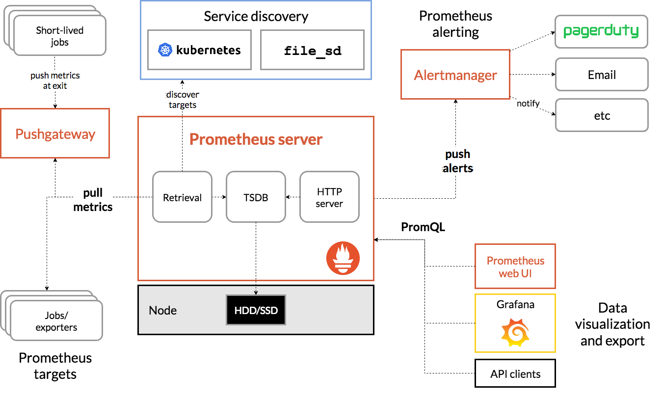
• the main Prometheus server which scrapes and stores time series data
• client libraries for instrumenting application code
• a push gateway for supporting short-lived jobs
• special-purpose exporters for services like HAProxy, StatsD, Graphite, etc.
• an alertmanager to handle alerts
• various support tools

Matienzo has a GitHub account with code that interacts with OCLC’s API

Is this really the extent of the connection between Matienzo and Anna’s Archive? I don’t know what is required at the Complaint stage of a civil lawsuit to prove someone is connected to an anonymous collective, but surely something more than this plus public statements and an internet handle (“anarchivist”) is required to convict. Does Ohio have SLAPP protections?

Author Response

Reviewer #1 (Public Review):

Weaknesses:

The manuscript needs proper editing and is not complete. Some wordings lack precision and make it difficult to follow (e.g. line 98 "we assembled a chromosome-scale genome of ..." should read instead "we assembled a chromsome-scla genome sequence of ...". Also, panel Figure 2E is missing.

We will make the suggested change of adding “sequence”. Concerning additional changes, we have carefully edited our manuscript and looked for any incomplete sections. Unfortunately, it is difficult to see what other issues are being raised here without any further information. And the example given is not helpful to ascertain what other changes may be necessary, since we cannot see any problem with the sentence “we assembled a chromosome-scale genome of” as this phrase is widely used in many similar publications.

As for panel E of figure 2, it is not missing. The panel located to the right, just below “Target Cells”.

The shortcomings of the manuscripts are not limited to the writing style, and important technical and technological information is missing or not clear enough, thereby preventing a proper evaluation of the resolution of the genomic resources provided:

• Several RNASeq libraries from different tissues have been built to help annotate the genome and identify transcribed regions. This is fine. But all along the manuscript, gene expression changes are summarized into a single panel where it is not clear at all which tissue this comes from (whole embryo or a specific tissue ?), or whether it is a cumulative expression level computed across several tissues (and how it was computed) etc. This is essential information needed for data interpretation.

No fertilised eggs or embryos have been sequenced, individual tissues derived from juvenile fish were used for the genome annotation and whole larval fish for the developmental analysis. We will specify in the figures and text that the results shown are from whole larvae, and add more detail to the material and methods section about which type of sample was analysed in which way.

• The bioinformatic processing, especially of the assemble and annotation, is very poorly described. This is also a sensitive topic, as illustrated by the numerous "assemblathon" and "annotathon" initiatives to evaluate tools and workflows. Importantly, providing configuration files and in-depth description of workflows and parameter settings is highly recommended. This can be made available through data store services and documents even benefit from DOIs. This provides others with more information to evaluate the resolution of this work. No doubt that it is well done,but especially in the field of genome assembly and annotation, high resolution is VERY cost and time-intensive. Not surprisingly, most projects are conditioned by trade-offs between cost, time, and labor. The authors should provide others with the information needed to evaluate this.

We will upload the code used to assemble and annotate this genome to a public repository or add it to the supplementary material.

The genome assembly did not use a specific workflow (e.g., nextflow), but was done with a simple command and standard parameters in IPA. Scaffolding was carried out by Phase Genomics using their standardised proprietary workflow, of which a detailed description provided by Phase Genomics can be found in the supplementary material. The annotation workflow has been described in a previous publication already, but an in-depth description can also be found in the Material and methods section, including parameters used for specific steps. The RNA-seq mapping and analysis part has also been described in the Material and Methods section, including parameters and models for DESEq2.

• Quantifications of T3 and T4 levels look fairly low and not so convincing. The work would clearly benefit from a discussion about why the signal is so low and what are the current technological limitations of these quantifications. This would really help (general) readers.

We will add a comment on this in the manuscript as suggested. Basically, the T3/T4 levels are consistent with other published work in fish. In the present manuscript for grouper we have a peak level of 1.2 ng/g (1,200 pg/g) of T4 and 0.06 ng/g (60 pg/g) of T3. This is a higher level of T4 and comparable level of T3 to what was found in convict tang (Holzer et al. 2017; Figure 2) with 30 pg/g of T4 and 100 pg/g of T3. Of course, there are also examples with higher levels, such as clownfish (Roux et al. 2023; Figure 1), with 10 ng/g (10,000 pg/g) of T4 and 2 ng/g (2,000 pg/g) of T3.

The differences could be due to different structure of fish tissues and therefore different hormone extraction efficiency, different hormone measurement protocols, different fish physiology, different fish size (e.g., the weighting of tiny grouper larvae is difficult and less precise than in convict tang). What is important is not the absolute level but the relative level, which shows the change within different larval stages of a species with identical extraction and measurement protocols. Which means our data is internally consistent and coherent with what the grouper literature says.

Holzer, Guillaume, et al. "Fish larval recruitment to reefs is a thyroid hormone-mediated metamorphosis sensitive to the pesticide chlorpyrifos." Elife 6 (2017): e27595.

Roux, Natacha, et al. "The multi-level regulation of clownfish metamorphosis by thyroid hormones." Cell Reports 42.7 (2023).

• Differential analysis highlights up to ~ 15,000 differentially expressed genes (DEG), out of a predicted 26k genes. This corresponds to more than half of all genes. ANOVA-based differential analysis relies on the simple fact that only a minority of genes are DEG. Having >50% DEG is well beyond the validity of the method. This should be addressed, or at least discussed.

As the reviewer notes, there are a large number of differentially expressed genes due to the fact that this is coming from a larval developmental transcriptome going from one day old larva to fully metamorphosed juveniles at around day 60.

While DESeq2 indeed works on an assumption that most genes are not differentially expressed, this affects normalization but not hypothesis testing (Wald-test, LRT tests or ANOVA). Normalisation in DESeq2 is fairly robust to this assumption. According to the author of DESeq2, Micheal Love, DESeq2 is using the median ratio for normalisation, and as long as the number of up and down regulated genes is relatively even, DESeq2 will be able to handle the data. As part of our general quality control for this project we consulted the MA plots, which do not show any overrepresented up or down expression patterns. Additionally see Michael Love comment on comparing different tissues, which is also applicable here when comparing vastly different larval stages (https://support.bioconductor.org/p/63630/): “For experiments where all genes increase in expression across conditions, the median ratio method will not be able to capture this difference, but this is typically not the case for a tissue comparison, as there are many "housekeeping" genes with relatively similar expression pattern across tissues.”

Reviewer #3 (Public Review):

Weaknesses:

However, the authors make substantial considerations that are not proven by experimental or functional data. In fact, this is a descriptive study that does not provide any functional evidence to support the claims made.

We agree with the reviewer that our paper lacks functional experiments but despite that, the transcriptomic data clearly show the activation of TH and corticoid pathways during two distinct periods; an early activation between D1 and D10, and a second one between D32 and juvenile stage. These data are interesting as they call for further examination of 1) the possible interaction of corticoids and TH during metamorphosis, a question that is certainly not settled yet in teleost fishes, and 2) the existence of an early larval developmental step also involving TH and corticosteroids.

Especially 2) is of interest and importance, since this early activation (unique to our knowledge in any teleost fish studied so far) raises a lot of new questions and once again will certainly be scrutinised by other groups in the years to come, therefore ensuring a good citation impact of our study. We hope that the reviewer, while disagreeing with some our statements, will recognize that our study will be stimulating at that level and that this is what scientific studies should do.

The consideration that cortisol is involved in metamorphosis in teleosts has never been shown, and the only example cited by the authors (REF 20) clearly states that cortisol alone does not induce flatfish metamorphosis. In that work, the authors clearly state that in vivo cortisol treatment had no synergistic effect with TH in inducing metamorphosis. Moreover, in Senegalensis, the sole pre-otic CRH neuron number decreases during metamorphosis, further arguing that, at least in flatfish, cortisol is not involved in flatfish metamorphosis (PMID: 25575457).

We will do our best to improve the clarity of the revised manuscript to avoid any misunderstanding about our claims. However, we would like to point out the semantic shift in the reviewer first sentence: Indeed “being involved” is not the same as “cortisol alone does not induce”. In ref 20 the authors explicitly wrote that “Cortisol further enhanced the effects of both T4 and T3, but was ineffective in the absence of thyroid hormones” and in our view this indeed corresponds to ”being involved in metamorphosis”.

We are not claiming that cortisol alone is involved in metamorphosis as the reviewer suggests, but simply that there is a possible involvement of cortisol together with TH in metamorphosis. We stand on this claim as we indeed observed an activation of corticoid pathway genes around D32, which is sufficient to say it is involved. We do agree that functional experiments will be needed to properly demonstrate the involvement of corticoids in grouper metamorphosis, but this was not possible in the current study as it would imply to set up a full grouper life cycle in lab conditions which is impossible for the scope of this manuscript.

We also mentioned in the discussion that the role of corticoids in fish larval development is still debated, and we agree that this remain a contentious issue.

We wrote that “there is contrasting evidence of communication between these two pathways [TH and corticosteroids] in teleost fish with some data suggesting a synergic and other an antagonistic relationship. In terms of synergy, an increase in cortisol level concomitantly with an increase in TH levels has been observed in flatfish (ref 19), golden sea bream (ref 100) and silver sea bream (ref 101). Cortisol was also shown to enhance in vitro the action of TH on fin ray resorption (phenomenon occurring during flatfish metamorphosis) in flounder (ref 20). TH exposure increases MR and GR genes expression in zebrafish embryo (ref 55). It has also been shown that cortisol regulates local T3 bioavailability in the juvenile sole via regulation of deiodinase 2 in an organ-specific manner (ref 56) On the antagonistic side, it has been shown that experimentally induced hyperthyroidism in common carp, decreasing cortisol levels (ref 57), whereas cortisol exposure decreases TH levels in European eel (ref 58). Given this scattered evidence, the existence of a crosstalk active during teleost metamorphosis has never been formally demonstrated. The results we obtained in grouper are clearly indicating that HPI axis and cortisol synthesis are activated (i) during early development and (ii) during metamorphosis. This may suggest that in some aspect cortisol synthesis can work in concert with TH, as has been shown in several different contexts in amphibians (ref 17).” In the revised manuscript, we will also add the interesting case of the Senegal sole mentioned by the reviewer.

In the last revision, we had also added that our results “brought a first insight into the potential role of corticoids in the metamorphosis of E. malabaricus and call for functional experiments directly testing a possible synergy” meaning that we clearly acknowledge that we are only revealing a hypothesis that remains to be tested. We later follow up with a discussion about the most novel observation and focus of our study, the increase in THs and cortisol during early development, which was unexpected and very intriguing. Again, these results suggest that there might be a link between the two, as has been shown in amphibians. This is typically the kind of results that should encourage more investigations into other fish species. Indeed, this has been pointed out by other authors and in particular by Bob Denver (probably the foremost expert on this topic) in Crespi and Denver 2012: “Elevation in HPA/I axis activity has been described prior to Metamorphosis in amphibians and fish, birth in mammals (reviewed in Crespi & Denver 2005a; Wada 2008)”. B. Denver also adds that: “Experiments in which GCs were elevated prior to metamorphosis or prior to hatching or birth (e.g. Weiss, Johnston & Moore 2007) or inhibited by treatments with GC synthesis blockers (e.g. metyrapone) or receptor antagonists (e.g. RU486, Glennemeir & Denver 2002) demonstrate that GCs play a causal role in precipitating these life-history transitions (also reviewed in Crespi & Denver 2005a; Wada 2008).” We believe the reviewer will be convinced by these elements coming from a colleague unanimously respected in the field.

Furthermore, the authors need to recognise that the transcriptomic analysis is whole-body and that HPA axis genes are upregulated, which does not mean they are involved in regulating the HPT axis. The authors do not show that in thyrotrophs, any CRH receptor is expressed or in any other HPT axis-relevant cells and that changes in these genes correlate with changes in TSH expression. An in-situ hybridisation experiment showing co-expression on thyrotrophs of HPA genes and TSH could be a good start. However, the best scenario would be conducting cortisol treatment experiments to see if this hormone affects grouper metamorphosis.

We agree that functional experiments are needed to validate our hypothesis. As the early peaks of expression levels observed for many genes were very intriguing for us, we did carry out thyroid hormones and goitrogenic treatment on young grouper larvae to test their effect on the morphological changes. Unfortunately, such experiments, already tricky on metamorphosing larvae, are even more risky on such tiny individuals just after hatching and we encountered high mortality rates. We must add that because we cannot establish a full grouper life cycle under lab conditions, we have done these experiment in the context of a commercial husbandry system in Japan, which while excellent limits the scope of possible experiments. We were thus not able to provide functional validation of our hypothesis. Such experiments will be a full project in itself, requiring setting up a rearing system suitable for both larval survival and economical constraints related to drug treatments. We were further limited by the spawning times of the grouper in the operational aquaculture farm, which are limited to a short time during each year. So even if we strongly agree with the necessity of conducting such experiments, we think that this is not in the scope of the present paper, but something future research can explore.

High TSH and Tg levels usually parallel whole-body TH levels during teleost metamorphosis. However, in this study, high Tg expression levels are only achieved at the juvenile stage, whereas high TSH is achieved at D32, and at the juvenile stage, they are already at their lowest levels.

This is exactly our point. We observe two peaks in TSH expression, one at D3 and one at D32. The peak at D3 coincides with high thyroid hormone levels on the same day, and while we have not measured TH at D32, existing literature shows that there is a peak in TH during that time (e.g., de Jesus et al., 1998). Similarly, there is a small peak of Tg at D3. Our manuscript focused more on the upregulation of these genes at D3, which has not been reported before in the literature and raised the question of the role of TH so early in the larval development, outside of the metamorphosis period.

Regarding the respective levels of TSH and Tg, we first would like to add that their respective order of appearance before metamorphosis (TSH at D32, Tg after) is consistent with what we would expect. We agree however that the strong increase of Tg and TPO expression is later than expected. We will make this clear in the revised manuscript.

It is very difficult to conclude anything with the TH and cortisol levels measurements. The authors only measured up until D10, whereas they argue that metamorphosis occurs at D32. In this way, these measurements could be more helpful if they focus on the correct developmental time. The data is irrelevant to their hypothesis.

We respectfully disagree with the reviewer, considering that 1) TH levels have already been investigated in groupers coinciding with pigmentation changes and fin rays resorption, 2) that there is also evidence in numerous fish species that TH level increase is concomitant with increase of TH related genes, and 3) that we observed in our data an increase in the expression of TH related genes as well as pigmentation changes and fin rays resorption. Based on our experience in fish metamorphosis and the literature we can say confidently that those observations indicate that metamorphosis is occurring between D32 and the juvenile stage. To reinforce our point, we plan to add a figure to the revised manuscript, which puts our data in the context of earlier studies done in grouper. This will clearly show that our inference is correct. Additionally, we would like to point out that from our experience in several fish species transcriptomic data are more robust and precise than hormone measurements.

However, as we were surprised by the activation of TH and corticoid pathway genes very early in the larval development (at D3), which is clearly outside of the metamorphosis period, we decided to measure TH and cortisol levels during this period of time to determine if whether or not there this surprising early activation was indeed corresponding to an increase in both TH and cortisol. As such observation has never been made in other teleost species (to our knowledge), and as we were wondering if gene activation was accompanied by hormonal increase, the measurements we did for TH and cortisol between D1 and D10 are relevant. We will make sure to improve the clarity of the revised version of the manuscript to avoid any confusion between the two periods we are studying: early larval development (between D1 and D10) and metamorphosis (between D32 and juvenile stage).

Moreover, as stated in the previous review, a classical sign of teleost metamorphosis is the upregulation of TSHb and Tg, which does not occur at D32 therefore, it is very hard for me to accept that this is the metamorphic stage. With the lack of TH measurements, I cannot agree with the authors. I think this has to be toned down and made clear in the manuscript that D32 might be a putative metamorphic climax but that several aspects of biology work against it. Moreover, in D10, the authors show the highest cortisol level and lowest T4 and T3 levels. These observations are irreconcilable, with cortisol enhancing or participating in TH-driven metamorphosis.

We thank the reviewer for this comment, but we think that there might be a misunderstanding here.

(1) We clearly observed an increase of TSHb (that occurs between D18 and juvenile stage) and an increase of tg from D32 which coincide with the activation of other genes involved in TH pathway (dio2, dio3, and also a strong increase of TRb). All this and put in the context of what we know from previous grouper studies, clearly supports our conclusion that TH-regulated metamorphosis is starting at around D32 in grouper. We also observed morphological changes such as fin rays resorption and pigmentation changes between D32 and juvenile stage. Such morphological changes have already been associated as corresponding to metamorphosis in groupers (De Jesus et al 1998) as they occur during TH level increase, and they also happen to be under the control of TH in grouper (De Jesus et al 1998). Based on this study but also on studies (conducted on many other teleost species) showing that the increase of TH levels is always associated with an activation of TH pathway genes and morphological and pigmentation changes we concluded that metamorphosis of E. malabaricus occurs between D32 and juvenile stage. We will improve the clarity of the manuscript to make sure that our conclusion is based on our transcriptomic and morphological data plus the available literature.

(2) We clearly observed another activation of TH related gene earlier in the development (between D1 and D10, with a surge of trhrs, tg and tpo at D3. As this activation was very unexpected for us, we decided to focus the analysis of TH levels between D1 and D10 and very interestingly we observed high level of T4 at D3 indicating that THs are instrumental very precociously in the larval development of the malabar grouper which has never been shown before. We declared line 195 that our “data reinforce the existence of two distinct periods of TH signalling activity, one early on at D3 and one late corresponding to classic metamorphosis at D32”. However, we agree that we could have been clearer and clearly explained that this early activation was very intriguing for us and that we wanted to investigate hormonal levels around that period. However, we never claimed anywhere in the manuscript that this early developmental period corresponds to metamorphosis. Something else is occurring and both TH and cortisol seem to be involved but further experiments need to be conducted to understand their role and their possible interaction.

(3) Finally, regarding the comment about cortisol enhancing or participating in TH driven metamorphosis, our data clearly showed an activation of the corticoid pathway genes around metamorphosis (between D32 and juvenile stage) suggesting a potential implication of corticoids in metamorphosis, but we agree with the reviewer that further experiment are needed to test that. We never claimed that cortisol was enhancing or participating in metamorphosis, on the contrary we are “suggesting a possible interaction between TH and corticoid pathway during metamorphosis”. And we also say that our “results brought a first insight into the potential role of corticoids in the metamorphosis of E. malabaricus and call for functional experiments directly testing a possible synergy.” Nonetheless, we agree that some parts of our manuscript can be confusing in regards of cortisol synthesis during metamorphosis as we did not measure cortisol levels between D32 and juvenile stage. We will correct this in the revised version.

Given this, the authors should quantify whole-body TH levels throughout the entire developmental window considered to determine where the peak is observed and how it correlates with the other hormonal genes/systems in the analysis.

We did not measure TH levels at later stages as it has already been measured during Epinephelus coioides metamorphosis and the morphological changes observed in this species around the TH peak corresponds to what we observed in Epinephelus malabaricus around the peak of expression of TH pathway genes (see De Jesus et al., 1998 General and Comparative Endocrinology, 112:10-16). We are planning to add a figure reconciling all these data together. However, the main focus of this manuscript is the novel observation of the existence of an early activation period observed at D3, and for which we needed TH levels to determine if they were involved in another early developmental process (not related to metamorphosis). Our hypothesis is that this early activation might be related to the growth of fin rays necessary to enhance floatability during the oceanic larval dispersal. As we may have arrived at the explanation of this hypothesis too rapidly without setting up the context well enough, we will pay attention to improve that part too.

Even though this is a solid technical paper and the data obtained is excellent, the conclusions drawn by the authors are not supported by their data, and at least hormonal levels should be present in parallel to the transcriptomic data. Furthermore, toning down some affirmations or even considering the different hypotheses available that are different from the ones suggested would be very positive.

We thank the reviewer for acknowledging the solidity of the method of our paper and the quality of the results. We agree that there were several parts where our message is unclear, which we will address in the revised version of the manuscript to make sure there is no more confusion between the two distinct periods we studied in this paper (early larval development and metamorphosis). We will also make sure that our claims about TH/corticoids interaction during both periods remain hypothetical as we cannot yet, despite trials, sustain them with functional experiment.

Résumé de la vidéo [00:00:00][^1^][1] - [00:23:39][^2^][2]:

Cette vidéo présente une conférence sur l'avenir des transports, en se concentrant sur le véhicule autonome. Patrick Perez, directeur scientifique chez Valeo, discute des avantages et des défis de cette technologie, en soulignant son potentiel pour améliorer la sécurité, le confort et l'efficacité des transports. Il aborde l'histoire du véhicule autonome, les progrès techniques, les niveaux d'automatisation et les défis techniques tels que la perception, la prédiction et la prise de décision.

Points forts: + [00:00:22][^3^][3] Introduction de la conférence * Présentation de Patrick Perez * Discussion sur le véhicule autonome + [00:02:31][^4^][4] Histoire et développement * Projet Prometheus en Europe * Challenges DARPA aux États-Unis + [00:05:12][^5^][5] Évolution récente et acteurs clés * Transition de Google Car à Waymo * Concurrence internationale dans le domaine + [00:07:14][^6^][6] Diversité des véhicules autonomes * Véhicules de livraison, navettes autonomes * Camions et équipements agricoles + [00:11:08][^7^][7] Niveaux d'automatisation * Explication des différents niveaux * Importance de la sécurité et de la légalité + [00:13:00][^8^][8] Défis techniques et solutions * Perception, prédiction et décision * Utilisation de l'intelligence artificielle et des capteurs Résumé de la vidéo [00:23:43][^1^][1] - [00:35:24][^2^][2]:

La partie 2 de la vidéo aborde les avancées dans les systèmes de transport, en mettant l'accent sur les véhicules autonomes et l'intelligence artificielle. Elle explique le rôle des capteurs, l'importance des données pour l'entraînement des modèles d'IA, et les défis liés à la fiabilité et la certification des systèmes automatisés.

Points forts: + [00:23:43][^3^][3] Les capteurs et la loi * Importance de respecter le code de la route et les lois de la physique * Présentation des différents types de capteurs utilisés dans les véhicules + [00:25:00][^4^][4] Perception et adaptation * Les capteurs ont des résolutions et des modes de fonctionnement variés * Adaptation de domaine pour améliorer la perception des systèmes d'IA + [00:28:08][^5^][5] Prédiction de la confiance * Développement de réseaux de neurones pour prédire la confiance dans la détection * Importance de savoir quand le système ne sait pas pour une utilisation fiable + [00:30:23][^6^][6] Explicabilité des décisions * Problématique de l'interprétabilité des décisions des réseaux de neurones * Utilisation d'explications contrefactuelles pour comprendre les décisions d'IA

Résumé de la vidéo [00:00:00][^1^][1] - [00:21:47][^2^][2]:

Cette vidéo, présentée par Stanislas Dehaene, explore la perception des objets mathématiques élémentaires et leurs mécanismes cérébraux. Elle examine comment les humains reconnaissent rapidement des motifs géométriques et sonores, en utilisant des exemples comme les dessins géométrisés des enfants et les motifs anciens trouvés sur des objets datant de 70 000 à 100 000 ans. Dehaene discute de la capacité extraordinaire de percevoir des motifs abstraits et comment cela est traité dans le cerveau, en s'appuyant sur des études comportementales et des modèles de langage de la pensée.

Points forts: + [00:00:26][^3^][3] Introduction au sujet * Focus sur les formes géométriques élémentaires * Importance des mécanismes cérébraux dans la perception + [00:01:41][^4^][4] Sensibilité aux motifs * Illustration avec une vidéo musicale * Reconnaissance immédiate des motifs spatiaux et sonores + [00:03:50][^5^][5] Étude des séquences géométriques * Utilisation d'un test avec des enfants pour étudier la perception * Capacité à anticiper des motifs géométriques complexes + [00:07:04][^6^][6] Langage de la géométrie * Nécessité d'un langage pour expliquer la mémoire des séquences * Présentation d'un modèle de langage de la pensée + [00:10:58][^7^][7] Performances et anticipation * Corrélation entre la complexité des séquences et la performance * Étude des mouvements oculaires et de l'IRM fonctionnelle + [00:16:09][^8^][8] Inférence de programme * Exploration de la capacité à inférer des motifs géométriques * Discussion sur la nature des primitives du langage de la pensée Résumé de la vidéo [00:21:50][^1^][1] - [00:42:52][^2^][2]:

La partie 2 de la vidéo se concentre sur la perception des objets mathématiques élémentaires et leur représentation dans le cerveau. Stanislas Dehaene explore les régions cérébrales activées par les tâches géométriques et mathématiques, la magnéto-encéphalographie pour suivre l'activité cérébrale, et comment les séquences spatiales sont codées et anticipées par le cerveau. Il discute également des limites de la compréhension des séquences spatiales chez les animaux par rapport aux humains.

Points saillants: + [00:22:00][^3^][3] Activation cérébrale et langage * Les régions activées par le langage ne sont pas les mêmes que celles utilisées pour les tâches géométriques * Les tâches géométriques activent des régions liées au calcul mental * L'anticipation cérébrale joue un rôle dans la complexité des séquences + [00:23:25][^4^][4] Magnéto-encéphalographie * Permet de suivre l'activité cérébrale milliseconde par milliseconde * Révèle comment le cerveau code et anticipe les séquences spatiales * Montre que le cerveau fonctionne sur un mode prédictif + [00:27:01][^5^][5] Anticipations cérébrales * Le cerveau anticipe les positions dans les séquences avant qu'elles ne surviennent * La capacité d'anticipation est corrélée avec la complexité de la séquence * Les représentations mentales abstraites comme la rotation et la symétrie sont décodables + [00:33:00][^6^][6] Comparaison avec les animaux * Les animaux ont des difficultés à comprendre les structures géométriques complexes * Les humains ont une capacité unique à former des structures récursives et à comprimer l'information * Cette capacité pourrait être propre à l'espèce humaine Résumé de la vidéo [00:42:54]¹[1] - [01:03:55]²[2]:

Cette partie de la vidéo explore la perception des objets mathématiques élémentaires dans la musique et la géométrie, en se concentrant sur la théorie de la compression de l'information et son application dans la compréhension des séquences musicales et géométriques. Stanislas Dehaene discute de l'ancienneté du phénomène musical chez Homo sapiens, comparable à celle du langage géométrique, et présente des expériences de laboratoire simplifiant ces phénomènes pour tester la mémoire de travail et la détection de régularités.

Points saillants: + [00:42:54]³[3] Ancienneté de la musique et de la géométrie * Présentation de flûtes anciennes comme preuve de la culture musicale préhistorique * Comparaison de l'ancienneté du langage musical avec le langage géométrique + [00:43:36]⁴[4] Expériences de laboratoire sur la musique * Utilisation de séquences musicales binaires pour tester la mémoire et la perception des régularités * Proposition d'un système de compression de l'information pour les séquences musicales + [00:45:01]⁵[5] Complexité des séquences musicales * Discussion sur la longueur de description minimale et la complexité subjective perçue * Exclusion de modèles alternatifs et confirmation de la théorie de la compression + [00:49:55]⁶[6] Systèmes de règles et statistiques dans la perception * Distinction entre le traitement des règles et des statistiques dans la perception des séquences * Présentation d'un modèle bayésien pour inférer les règles et les probabilités de transition

Source : conversation avec Bing, 14/03/2024 (1) undefined. https://www.education.gouv.fr/education-la-sexualite-en-milieu-scolaire-341103. (2) undefined. https://soseducation.org/docs/notes-etudes-entretiens-tribunes/education-a-la-sexualite-danger-ou-prevention-final.pdf. (3) undefined. https://www.planning-familial.org/sites/default/files/2023-11/LIVRE_BLANC_WEB.pdf. (4) undefined. https://www. Résumé de la vidéo [01:03:56][^1^][1] - [01:21:55][^2^][2]:

Cette partie de la vidéo aborde la perception des objets mathématiques élémentaires à travers une étude sur la structure des séquences musicales et leur traitement cérébral. Stanislas Dehaene discute des résultats d'IRM montrant comment le cerveau humain traite la complexité des séquences musicales, révélant un réseau de régions cérébrales impliquées dans la compréhension de la structure et de la syntaxe des séquences.

Points saillants: + [01:03:56][^3^][3] Traitement des séquences musicales * Étude des parenthèses placées par les sujets dans des séquences * Révélation de la structure perçue par le cerveau * Différences entre séquences simples et complexes + [01:05:11][^4^][4] Résultats d'IRM et prédiction de la complexité * Activation cérébrale croissante avec la complexité des séquences * Réseau de régions cérébrales associées à la perception de la structure * Inversion de l'activation pour les séquences complexes + [01:07:55][^5^][5] Séparation entre musique et langage * Études indiquant une distinction claire dans le cortex temporal supérieur * Régions cérébrales spécialisées pour le traitement du langage et de la musique * Peu de recouvrement entre les aires du langage et celles traitant la musique + [01:11:56][^6^][6] Implications en éducation et mathématiques * Corrélation entre la capacité de traiter les motifs et les performances mathématiques * Potentiel impact de l'entraînement musical sur le développement des compétences abstraites * Importance de l'enseignement précoce des motifs géométriques et musicaux

Author Response

The following is the authors’ response to the original reviews.

Reviewer #1

More details about the classification and how it is trained

We included a sentence in the introduction to clarify which data we are using: "In order to demonstrate this improvement, we apply our methods to two classification datasets: a synthetic dataset and a public clinical dataset where the predicted outcome is the survival of the patient"

And about how the classifier is trained in the "Results" section: "we used the default parameters of the classifier, since our focus is comparing the different imputation methods"

Availability of the code

Now the code is publicly available in a github repository https://github.com/AstraZeneca/dpp_imp/ (see Availability of Data and Code section)

Reviewer #2

Clarifying that Determinantal Point Processes and their deterministic version have been introduced before but are applied for the first time for data imputation in this work:

We added explanation in the 6th paragraph of the introduction that we use pre-existing DPP and deterministic-DPP algorithms for our imputation methods and include the references to avoid confusion

We also added a paragraph at the end of the introduction to summarize this work's contribution

Explaining the claim about the computational advantage of using quantum determinantal point processes for the imputation methods:

In the fourth paragraph of the "Discussion" section (page 8), we give an imputation example by numerically comparing the classical and quantum algorithms running time for DPP sampling, which shows the advantage of using the quantum algorithm.

Regarding running time for classical DPP and quantum DPP sampling algorithms:

We included Table VIII (page 13) that compares the preprocessing and sampling complexities for both classical and quantum DPP algorithms, we consider the case where we sample d rows from an (n,d) matrix and n=O(d) which is usually the case for our DPP-Random Forest algorithm

We added some details regarding the quantum advantage in the first paragraph of page 12

Regarding the comment about the modest improvement of the DPP methods and questions about their practical benefit:

As mentioned in the third paragraph of the "Discussion" section, we point out that the consistency of the improvement and the removal of variance as a result of using the DPP and deterministic DPP methods make our methods very beneficial to use on clinical data. Further exploration with different data sets can provide a more result in a more complete understanding of the practical advantages of the methods

Algorithmic complexity of the deterministic DPP algorithm:

Detailed in the last sentence of the "Determinantal Point Processes" subsection of the "Methods" section: O(N^2 d) for the preprocessing step and O(Nd^3) for the sampling step

Running time for the quantum deterministic DPP sampling and how it is done in practice:

While it is difficult to assess the real running time for the quantum detDPP algorithm for large circuits (100 or more qubits), due to the unavailability of such devices, we give more details about our practical implementation in the last paragraph of the "Methods" section. In our case (up to 10 qubits) we used 1000 shots to sample the highest probability elements.

On which quantum simulator was used

We point out in the first paragraph of page 5 that we employ the qiskit noiseless simulator

References

Bansal R, Nagel M, Stopkova R, Sofer Y, Kimchi T, Stopka P, Spehr M, Ben-Shaul Y. 2021. Do all mice smell the same? Chemosensory cues from inbred and wild mouse strains elicit stereotypic sensory representations in the accessory olfactory bulb. BMC Biol 19:133.
Ben-Shaul Y, Katz LC, Mooney R, Dulac C. 2010. In vivo vomeronasal stimulation reveals sensory encoding of conspeciic and allospeciic cues by the mouse accessory olfactory bulb. Proc Natl Acad Sci U S A 107:5172‒5177.
Bergan JF, Ben-Shaul Y, Dulac C. 2014. Sex-speciic processing of social cues in the medial amygdala. Elife 3:e02743.
Engelke DS, Zhang XO, OʼMalley JJ, Fernandez-Leon JA, Li S, Kirouac GJ, Beierlein M, Do-Monte FH. 2021. A hypothalamic-thalamostriatal circuit that controls approachavoidance conlict in rats. Nat Commun 12:2517.
Esteban Masferrer M, Silva BA, Nomoto K, Lima SQ, Gross CT. 2020. Differential Encoding of Predator Fear in the Ventromedial Hypothalamus and Periaqueductal Grey. J Neurosci 40:9283‒9292.
Papes F, Logan DW, Stowers L. 2010. The vomeronasal organ mediates interspecies defensive behaviors through detection of protein pheromone homologs. Cell 141:692‒703.
Tobias BC, Schuette PJ, Maesta-Pereira S, Torossian A, Wang W, Sethi E, Adhikari A. 2023. Characterization of ventromedial hypothalamus activity during exposure to innate and conditioned threats. Eur J Neurosci 57:1053‒1067.