Always use a while read construct: find . -name "*.txt" -print0 | while read -d $'\0' file do …code using "$file" done The loop will execute while the find command is executing. Plus, this command will work even if a file name is returned with whitespace in it. And, you won't overflow your command line buffer.
10,000 Matching Annotations
- Jul 2022
-
stackoverflow.com stackoverflow.com
-
-
What ever you do, don't use a for loop: # Don't do this for file in $(find . -name "*.txt") do …code using "$file" done Three reasons: For the for loop to even start, the find must run to completion. If a file name has any whitespace (including space, tab or newline) in it, it will be treated as two separate names. Although now unlikely, you can overrun your command line buffer. Imagine if your command line buffer holds 32KB, and your for loop returns 40KB of text. That last 8KB will be dropped right off your for loop and you'll never know it.
-
-
-
in a real Redux app, we're not allowed to import the store into other files, especially in our React components, because it makes that code harder to test and reuse.
I don't understand this, because we could still call
react-redux'suseDispatchto get the store's dispatcher, couldn't we?
-
-
web.hypothes.is web.hypothes.is
-
Review with care and humanity Code reviews are business-critical—all production code requires review—and an important opportunity to support your teammates. Everyone involved, whether author or reviewer, has one core objective: help to move things forward. As a reviewer, you are a partner in the success of the body of work. Make code reviews a top priority, and be thorough and compassionate. Commit yourself when you review: focus and take your time. Avoid dismissive terms like “simply”, “just.” Ask questions. Discuss the code, not the coder. There are many conventions and techniques at play in high-quality code reviews, but all involve common underpinnings: be responsive, be committed and be kind. If you’re the code author, set your reviewer up for the best possible review cycle. Roll out the red carpet with a polished PR description. Do everything you can so that your reviewer can get down to the work of reviewing without fuss. Screenshots. Testing instructions. Comments to help them navigate. Remember to expect feedback—that’s the whole point—and to respond to it with the same humanity you expect from your reviewer.
-
-
github.com github.com
-
// switch (randomItem) { // case 1: // return SCR; // case 2: // return PAP; // case 3: // return STN; // default: // break; };
yes! definitely! switch case statements would be a good use case. makes code much more readable as well
-
-
betasite.razorpay.com betasite.razorpay.com
-
string The ifsc code of your bank account.
Webhook?
-
-
gist.github.com gist.github.com
-
var main = function (userInput) { var programHand = randomProgramHand(); var userHand = userInput; var outcome = gameSPS(userHand, programHand); if (outcome == "win") { numPlayerWins += 1; totalGamesPlayed += 1; return winMssg(programHand, userHand, numPlayerWins, totalGamesPlayed); } else if (outcome == "lose") { totalGamesPlayed += 1; return loseMssg(programHand, userHand, numPlayerWins, totalGamesPlayed); } else if (outcome == "tied") { totalGamesPlayed += 1; return tiedMssg(programHand, userHand, numPlayerWins, totalGamesPlayed); } else if (outcome == "error") { return "Please key in 'scissors' 'paper' or 'stone' and try again"; } };
good that ur main function is short and u make use of helper functions. make ur code easier to read
-
-
cbloomrants.blogspot.com cbloomrants.blogspot.com
-
xample code should never be sketches. It should be production ready.
Example code isn't cheap or quick - no matter how you represent it, this code sets the tone for canonical project use. If it's not properly written then (1) the library should be simple enough to make the canonical usage obvious, so you've messed up, and (2) you should spend more time using your library to understand how to make it both idiomatic and intuitive.
-
-
docdrop.org docdrop.org
-
can extract a procedure from open code we start by selecting a piece of code that we think might be shareable we apply the enzyme and we get a procedure and a call to it with all the necessary
parameters formal and actual
extract a procedure
-
-
www.feat.engineering www.feat.engineering
-
the ZIP code also qualifies as a qualitative predictor because the numeric values have no continuous meaning.
Esto es equivalente a la zona y por lo tanto se debe codificar como factor.
-
-
www.redditinc.com www.redditinc.com
-
Upload, transmit, or distribute to or through the Services any viruses, worms, malicious code, or other software intended to interfere with the Services, including its security-related features;
Smart, I like that reddit explicitly states it will not tolerate the use of its service as a promoter for malware. However, I have seen some sketchy posts on reddit with some questionable links so I don't know how effective it is at moderating this term.
-
-
addyosmani.com addyosmani.com
-
Deep modules Write code that solves complex problems for other developers but exposes functionality through a lucid interface.
this resonates a lot, also matches what I read in the book <philosophy of software design>, a package / module should be deep, so that it offers something that can really help
-
-
-
optimizing packaging size will improve cold start performance. - use aws sdk v3 - bundle and minify code - avoid top-level import
-
-
reactjs.org reactjs.org
-
wrap it in a call to React.memo
I was wondering whether this should be done in the module defining and exporting the component, or in the code consuming it.
Given that
React.memocould be thought of as a replacement ofPureComponentfor function components, I think it would be appropriate to have the module export the wrapped version of the component.
-
-
www.biorxiv.org www.biorxiv.org
-
Abstract
This work has been published in GigaByte Journal under a CC-BY 4.0 license (https://doi.org/10.46471/gigabyte.64), and has published the reviews under the same license. These are as follows.
Reviewer 1. Peter Mulhair
Is the language of sufficient quality?
This manuscript is clear and concise. However, there are some issues with consistency in species names used throughout the manuscript. First, on line 99 Eubasilissa regina should be italicised. Secondly, I would recommend after the initial use of the full names of the species (Plodia interpunctella and Eubasilissa regina) that these be referred to as P. interpunctella and E. regina in the rest of the text. There is inconsistent use of full species names, shortened species names and genus name alone which may cause confusion. Please read through and correct these inconsistencies throughout the manuscript text.
Are the data and metadata consistent with relevant minimum information or reporting standards? See GigaDB checklists for examples http://gigadb.org/site/guide
No. Missing items from the metadata checklist include (1) Coding gene annotations (GFF), Coding gene nucleotide sequences and Coding gene translated sequences (fasta) and (2) Full (not summary) BUSCO results output files (text).
Is the data acquisition clear, complete and methodologically sound?
Yes. Is there a specific reason why fifth instar larvae were used for RNA sequencing of silk glands of P. interpunctella? If this stage is biologically important than it may be worth stating why this specific stage is used.
Is there sufficient detail in the methods and data-processing steps to allow reproduction?
Yes. However, the code used for Heavy fibroin gene annotation could be made publicly available to enable reproducibility of this analysis (using other species for example or to annotate other repeat rich genes). This could be uploaded to the rest of the relevant code at https://github.com/AshlynPowell/silk-gene-visualization
Is there sufficient information for others to reuse this dataset or integrate it with other data?
Yes. One point worth making is that on Line 161 you state that "The assembly for E. regina is the most contiguous Trichoptera genome assembly to date.". However, there are currently 3 chromosome level assemblies available for Trichoptera on NCBI. I would recommend removing this statement, or changing it by also pointing to these other genomes available.
Other comments:
This work was carried out to a very high quality and I am particularly happy to see more high quality genomic and transcriptomic data for these groups of insects. I also think that annotation of the Heavy fibroin genes is of particular importance and relevance to researchers interested in silk evolution and evolution and annotation of repeat rich proteins.
Recommendation: Minor revision
Reviewer 2. Reuben W Nowell
Are all data available and do they match the descriptions in the paper?
No. I wasn't able to access the data with the FTP link provided.
Additional comments:
A very nice piece of work, I have only a few minor comments:- Line 140: "with the k-mer length set to 1" - do you mean 21?
- Line 164: great that you provide a link to the GenomeScope html but I recommend to add these kmer plots as additional supplemental figures, they are extremely useful. Just a screenshot of the GenomeScope plot would be fine.
- Line 164: in relation to the kmer distributions, in fact both plots look a little bit multimodal to me... especially the Eubasilissa, with peaks at 1n (20x), 2n (40x) and 4n (~80x) coverage. This might indicate tetraploidy, which might explain the large increase in genome span and gene number for this species too. You could run OrthoFinder and look at the distribution of OG membership size, for diploid assemblies it peaks at 2, but you might find a peak at 2 and 4 for Eubasilissa if it is tetraploid.
- Line 167: how many contaminant contigs were identified, and where did they come from? - Line 168: the coverage for both species is roughly the same, but the species with the much larger genome is the more contiguous one - any ideas why this is the case?
- Line 184: maybe this is a silly question, but how do you know they are full-length? Based on the B. mori BAC sequence?
- Line 192: a unit for molecular weight, Da?
- Line 224: would be useful to know how many genes are in the Insecta core BUSCO db (i.e., where the 95% comes from).
- Line 233: is there a possibility that RepetModeler has also classified the repeat-rich fibroin genes as 'repeats', and so these are masked in the assemblies?
- Line 243: this is a huge difference in gene number! Why? Is the E. regina assembly actually a diploid assembly? Or ploidy > 2? [See above comment on kmer plots].
- Line 265: "insects have generally been neglected with respect to genome sequencing efforts" - quite a bold statement and I'm not sure I agree, there has been a huge focus on lepidopteran genomics and much of the early sequencing from initiatives such as Darwin Tree of Life have been on insects (also i5k).
- Line 457: Table 2: any idea why the P. interpunctella HiFi assembly is ~60 Mb shorter than the two Illumina assemblies?
- Line 475: Figures 2 and 3: these are nice figures but I don't quite follow what the two coloured panels on the left are showing, specifically, why are there two panels? A bit more clarification in the legend needed perhaps.
- Line 476: N and C capitalised
Recommendation: Minor revision
Reviewer 3. Martin Pippel
Is there sufficient information for others to reuse this dataset or integrate it with other data?
Yes. (partly) : To make the study fully reproducible the authors need to upload the PacBio HiFi data (e.g. to NCBI). Otherwise the genome assemblies cannot be reproduced with the available raw data in GenBank.
Any additional comments:
The manuscript entitled “Long-read HiFi sequencing correctly assembles repetitive heavy fibroin silk genes in new moth and caddisfly genomes” from Kawahara et al. describes the de novo assembly and gene annotation of two silk-producing insect species Plodia interpunctella and Eubasilissa regina. The manuscript is well structured and written. Sequencing data, assemblies and genome annotations are publicly available and can be reused by the scientific community. Both contig assemblies show a very high contiguity and good BUSCO scores. Indeed, several from the 118 P. interpunctella and 53 E. regina contigs show telomere repeat sequence at both ends indicating that those represent full chromosomes. Furthermore, the authors showed that even long repetitive genes such as silk fibroin genes were gapless assembled. I consider the manuscript as a valuable contribution for the scientific community and do only have some minor comments and suggestions:line 129: - which CCS version was used? line 140: - k-mer length was set to 1? Not 21? line 148: - Typo: obd10 reference endopterygota. - In order to make the Busco scores better comparable to other recent Lepidoptera assemblies it would be better to provide the BUSCO scores for P. interpunctella based on the lepidoptera lineage line 158: CCS data should be added to GenBank as well. Usually the raw data (subreads.bam) is lossy converted into fastq files from NCBI, which makes it impossible to reproduce the consensus step with pbCCS or even the assembly. line 159: Both read coverages are quite high and the heterozygosity rates are with 0.7 (Eubasilissa) and 0.36 (Plodia) high as well. I was wondering if the alternate assemblies were also of a decent quality and if those are published as well? line 265: As of today, there are at least 3 other HiFi assemblies available: (GCA_917563855.2, GCA_929108145.1, GCA_917880885.1) line 457: Table 2 states that E.regina was assembled into 53 contigs. However the assembly available at NCBI GCA_022840565.1 has 123 contigs!?
-
-
www.usenix.org www.usenix.org
-
Of course letting arbitrary code potentially run forever wouldn’t work. So instead any program is run for only a limited number of instructions until it either completes or is terminated. The measure of the amount of compute is called “gas”, with various instructions and operations costing a different amount of gas to process. The total cost of a transaction is the amount of gas consumed times the gas price.
Definition of "gas" on the blockchain
-
-
github.com github.com
-
Thanks for your making your first contribution to Cucumber, and welcome to the Cucumber committers team! You can now push directly to this repo and all other repos under the cucumber organization! In return for this generous offer we hope you will: Continue to use branches and pull requests. When someone on the core team approves a pull request (yours or someone else's), you're welcome to merge it yourself. Commit to setting a good example by following and upholding our code of conduct in your interactions with other collaborators and users. Join the community Slack channel to meet the rest of the team and make yourself at home. Don't feel obliged to help, just do what you can if you have the time and the energy. Ask if you need anything. We're looking for feedback about how to make the project more welcoming, so please tell us!
-
-
www.econometrics-with-r.org www.econometrics-with-r.org
-
# Create the dummy variable as defined above CASchools$D <- CASchools$STR < 20 # Plot the data plot(CASchools$D, CASchools$score, # provide the data to be plotted pch = 20, # use filled circles as plot symbols cex = 0.5, # set size of plot symbols to 0.5 col = "Steelblue", # set the symbols' color to "Steelblue" xlab = expression(D[i]), # Set title and axis names ylab = "Test Score", main = "Dummy Regression")
If you want to reproduce the exact plot you need to run the following code:
           CASchools$D <- CASchools$STR < 20                                   # Create the dummy variable as defined above

    mean.score.for.D.1 <- mean( CASchools$score[ CASchools$D == TRUE  ] )      # Compute the average score when D=1 (low  STR)
    mean.score.for.D.0 <- mean( CASchools$score[ CASchools$D == FALSE ] )      # Compute the average score when D=0 (high STR)


    plot( CASchools$score ~ CASchools$D,                                       # Plot the data

                 pch = 19,
                 cex = 0.5,
                 col = "Steelblue",
                xlab = expression(D[i]),
                ylab = "Test Score",
                main = "Dummy Regression")

    points( y = mean.score.for.D.0, x = 0,   col="red", pch = 19)               # Add the average for each group
    points( y = mean.score.for.D.1, x = 1,   col="red", pch = 19)
-
-
www.medrxiv.org www.medrxiv.org
-
Author Response:
Reviewer #1 (Public Review):
The authors show that the unmitigated generation interval of the original variant of SARS-CoV-2 is longer than originally thought. They argue that in the absence of interventions that limit transmission late in the course of infection, the fraction of transmission events that occur before symptom onset would be considerably lower, and the fraction of transmission events occurring 10 days or more after infection of the index case would be substantially higher.
These findings improve our ability to accurately estimate the basic reproductive number (R0), to evaluate quarantine and isolation policies, and to model counterfactual intervention-free scenarios. Many applied analyses rely on accurate generation interval estimates. To head off confusion, it would be helpful if the authors could provide more comprehensive guidance about which applied analyses should be informed by the unmitigated generation interval, or the observed generation interval. (E.g. the unmitigated interval is useful for quarantine and isolation policies, but would we ever want to use the unmitigated interval to estimate R?).
The unmitigated generation-interval should be used for estimation of the R0 of the initial epidemic phase, but not for the R(t) of the current epidemics. Estimation of R(t) must account for changes in generation-interval distributions caused by the invasion of new variants and changes in behavior. When analyzing policies of quarantine, isolation or contact tracing, the unmitigated interval should also be adopted to account for late transmissions.
We added few sentences at the end of our introduction to clarify this point:
“The estimated unmitigated generation-interval distribution could be adopted for answering questions about quarantine and isolation policy, as well as for estimating the original R0 at the initial spread in China. However, estimation of instantaneous R(t) should account for changes in generation-interval distributions, reflecting mitigation effects and the current variant.”
The analysis estimates a longer generation interval after accounting for three main sources of bias or error that are common in other analyses: 1. Recently infected individuals are intrinsically overrepresented in data on a growing epidemic. Thus, shorter incubation periods and forward serial intervals are more likely to be observed, even in the absence of interventions. This analysis adjusts for these dynamical biases. 2. Interventions or behavioral changes can prevent transmission late in the course of infection. This can shorten the generation and serial intervals over the course of an epidemic. This analysis focuses specifically on transmission pairs observed very early, before the adoption of interventions. 3. The incubation period and generation interval should be correlated - infectors that progress relatively quickly to symptoms should also become infectious sooner (symptom onset occurs near the peak of viral titers). Most existing analyses assume these intervals are uncorrelated, but this analysis accounts for their correlation.
Overall, the conclusions seem reasonable and well-supported. The observation that the generation interval decreases over the course of an epidemic is also consistent with existing studies that show the serial interval has similarly decreased over time. But given the implications of the findings, I hope the authors can address a few questions about potential additional sources of bias:
- It is somewhat reassuring that the generation interval decreases relatively smoothly as the cutoff date increases (Fig. S6), but it would be helpful if the authors address the potential impact of ascertainment biases. One of the main reasons that the authors estimate a shorter generation interval is that they define January 17th, early in the outbreak before interventions and behavioral changes had taken place, as the cutoff point for the infector's date of symptom onset. This cutoff eliminates biases from interventions, but it also severely limits the size of the transmission-pair dataset (Fig. S3), and focusing on this very early subset of cases may increase the influence of ascertainment bias. Prior to January 17th, should we expect observed transmission pairs to involve more severe cases on average? And is the unmitigated generation interval correlated with case severity?
We thank the reviewer for identifying a source of possible bias that we overlooked. Following the comment we performed a new sensitivity analysis for the inclusion of the severe cases, summarized in Appendix 1—figure 11.
Severity of the cases was reported only in Ali et al.’s data, for some of the individuals. In these cases, individuals are divided into one of three conditions: mild, severe (non-fatal) and death. As non-mild cases represent a small fraction of the dataset, we combine them into one category, which we denote as severe.
Severe cases (including deaths) were overrepresented in the period prior to January 17, with 8 out of 77 cases, compared to 18 out of 745 in the period of January 18-31. The effect of inclusion of severe cases was analyzed by comparing the means of the estimated generation-interval distribution, separately for the two periods in question, using the inference framework with 30 bootstrapping runs. For the earlier period, the estimated means were compared between the dataset with or without the severe cases. For the later period, we also consider the “enriched” dataset, in which severe cases are oversampled for each bootstrap such that the proportion of severe cases matches that during the earlier period (10%). In both cases we see that the effect on the estimated mean generation interval is small.
- The analysis assumes the incubation period follows a fixed distribution, whose parameterization comes from a meta-analysis of previously estimated incubation periods. But p.5 discusses the idea that observed incubation periods are affected by the same dynamical biases as forward serial intervals, "For example, when the incidence of infection is increasing exponentially, individuals are more likely to have been infected recently. Therefore, a cohort of infectors that developed symptoms at the same time will have shorter incubation periods than their infectees on average, which will, in turn, affect the shape of the forward serial-interval distribution." Has the incubation period been adjusted for these dynamical biases, or should it be?
In our analysis we use the incubation period distribution from Xin et al. 2021 which already considers the backward bias caused by the expanding epidemic with the corrected growth rate of 0.1/d. Xin et al. showed in their meta-analysis that the mean incubation period reported by the various sources changed according to the dates used by the source. Incubation periods prior to the peak of the epidemic in China were lower than ones from after the peak, in a manner that coincided with the backward correction they performed (using a similar derivation to that suggested by Park et al. 2021). Accordingly, the distribution of incubation period they report is the intrinsic incubation period, after correction for the growth rate of the initial spread in China. We added two sentences in our methods section to clarify this point:
“In their meta-analysis, Xin et al. found an increase of the incubation period following the introduction of interventions in China, matching the theoretical framework shown above. Their inferred incubation period distribution includes a correction for the growth rate of the early spread, accordingly.”
Furthermore, we perform a sensitivity analysis for the shape of the incubation period distribution, and show that it has a minor effect on our conclusions (Appendix 1—figure 10).
- It appears that correlation parameter estimates co-vary with estimates of the mean generation interval (Fig. S6; S13b). Are the authors confident that the correlation parameter is identifiable? How much would the median generation interval estimate in the main analysis change if the correlation parameter had been fixed to 0 (which isn't realistic) or to 0.5 (which might be plausible)?
As the reviewer pointed out, the correlation parameter estimates co-vary with estimates of the mean generation interval. We further analyzed this relation following the comment. The analysis is summarized in supplemental figures S19-20.
We first examine the relation between the mean generation interval and the correlation parameter based on the uncertainty estimates, consisting of 1000 bootstrap runs. Appendix 1—figure 12 shows a joint bivariate scatter plot of the parameters, together with contours of equal probability. As can be seen there is a connection between the parameters. The estimates centered around the maximum likelihood estimate with correlation parameter of 0.75 and mean generation interval of 9.7 days. The confidence interval for the correlation parameter of 0.45-0.95 corresponds to mean generation intervals in the range of 8-11 days, supporting the conclusion of this study.
Next, we reanalyzed the dataset while fixing the correlation parameter, as suggested by the reviewer. Appendix 1—figure 13 shows the estimated mean generation interval for fixed correlation parameters with values of 0, 0.25, 0.5, 0.75, 0.9. For each fixed correlation parameter 100 bootstrapping runs. As can be seen, the results reflect the same connection that can be seen in Appendix 1—figure 12, with probable values in the range of 8-11 days, for correlation parameters in the range of 0.5-0.9. Assuming no correlation would cause underestimation of the mean generation interval match previous literature (Hart, Maini, and Thompson 2021; Park et al. 2022).
Reviewer #2 (Public Review):
There have been several estimates of the generation time and serial interval published for SARS-CoV-2, but as the authors note, estimates can be subject to biases including shifted event timing depending on the phase of the epidemic, correlation in characteristics between infector and infectee, and impact of control measures on truncating potential infectiousness. This study, therefore, has several strengths. It first collates data on transmission events from the earliest phase of the COVID-19 pandemic, then makes adjustments for these potential biases to estimate the generation time in absence of control measures, and finally discusses implications for transmission.
Given many subsequent aspects of the COVID-19 pandemic have been defined relative to earlier phases (e.g. relative transmissibility of variants, relative duration of infectiousness), understanding the baseline characteristics of the infection is crucial. I thought this paper makes a useful contribution to this understanding, generating adjusted estimates for infectiousness (which is longer than previous estimates) and corresponding values for the reproduction number (which is remarkably similar to earlier estimates, presumably because of the different sources of bias in the growth rate and generation time distribution somehow end up canceling each other out).
However, there are some weaknesses at present. The study correctly flags several potential sources of bias in estimates, but in making adjustments uses estimates from the literature that themselves could suffer from these biases, e.g. the distribution of incubation period from a 2021 meta-analysis. Although the authors conduct some sensitivity analysis it would be worth including some more explicit consideration of whether they would expect any underlying bias to propagate through their calculations. The authors also conduct some sensitivity analysis around the underlying data (e.g. ordering of transmission pairs), but again it would be useful to know whether there could be systematic biases in these early data. Specifically, the paper references Tsang et al (2020), which highlighted variability in early case definitions - is it possible that early generation times are estimated to be longer because intermediate cases in the transmission chain were more likely to go undetected than later in the epidemic?
We recognize the potential biases in the transmission pairs data. We therefore developed an extensive framework of sensitivity analyses for identifying biases that could substantially affect the results. In the results section and figure 5, we show that the main study result, that the unmitigated generation-interval distribution is longer than previously estimated, is robust to reasonable amounts of ascertainment bias. We discuss this point at length and have added several supplemental figures to support this claim.
As reviewer #3 mentioned, we conducted a sensitivity analysis for the inclusion of the longest serial intervals, to investigate possible effects of missing links in the longest transmission pairs. We also discuss why we think it’s not necessary to explicitly model the short intervals that may be unobserved due to missing links.
“Second, we considered the possibility that long serial intervals may be caused by omission of intermediate infections in multiple chains of transmission, which in turn would lead to overestimation of the mean serial and generation intervals. Thus, we refit our model after removing long serial intervals from the data (by varying the maximum serial interval between 14 and 24 days). We also considered “splitting” these intervals into smaller intervals, but decided this was unnecessarily complex, since several choices would need to be made, and the effects would likely be small compared to the effect of the choice of maximum, since the distribution of the resulting split intervals would not differ sharply from that of the remaining observed intervals in most cases.”
We added to the discussion text regarding the effect of possible bias in the dataset, explicitly specifying the ascertainment bias.
“Our analysis relies on datasets of transmission pairs gathered from previously published studies and thus has several limitations that are difficult to correct for. Transmission pairs data can be prone to incorrect identification of transmission pairs, including the direction of transmission. In particular, presymptomatic transmission can cause infectors to report symptoms after their infectees, making it difficult to identify who infected whom. Data from the early outbreak might also be sensitive to ascertainment and reporting biases which could lead to missing links in transmission pairs, causing serial intervals to appear longer (For example, people who transmit asymptomatically might not be identified). Moreover, when multiple potential infectors are present, an individual who developed symptoms close to when the infectee became infected is more likely to be identified as the infector. These biases might increase the estimated correlation of the incubation period and the period of infectiousness. We have tried to account for these biases by using a bootstrapping approach, in which some data points are omitted in each bootstrap sample. The relatively narrow ranges of uncertainty suggest that the results are not very sensitive to specific transmission pairs data points being included in the analysis. We also performed a sensitivity analysis to address several potential biases such as the duration of the unmitigated transmission period, the inclusion of long serial intervals in the dataset, and the incorrect ordering of transmission pairs (see Methods). The sensitivity analysis shows that although these biases could decrease the inferred mean generation interval, our main conclusions about the long unmitigated generation intervals (high median length and substantial residual transmission after 14 days) remained robust (Figure 5).”
It would also be helpful to have some clarifications about methodology, particularly in how the main results about generation time are subsequently analyzed. For example, estimates such as the conversion of generation time to R0 and VOC scalings are described very briefly, so it is currently unclear exactly how these calculations are being performed.
Following the reviewer comments we made edits to the Methods section in order to make it more readable and clearer. We added subheadings for the various sections. Moreover, we added a section explaining the derivation of the basic reproduction number and clarified the section regarding the VOCs extrapolations.
We made some edits to the methods section in order to make it more accessible and clear, for example, we added subheadings for the various sections, added a section explaining the derivation of the basic reproduction number, and clarified the section regarding the VOCs extrapolations.
Reviewer #3 (Public Review):
Sender & Bar-On et al. perform robust analyses of early SARS-CoV-2 line list data from China to estimate the intrinsic generation interval in the absence of interventions. This is an important topic, as most SARS-CoV-2 data are from periods when transmission-reducing interventions are in place, which will lead to underestimation of the potential infectious period.
The authors highlight two shortcomings in previous approaches. First, the distribution of 'observed' serial intervals (the time between symptom onset in the infector and symptom onset in the infectee) depends not only on the timeline of each infector's infection, but also the epidemic growth rate, which weights the proportion of observed short vs. long serial intervals. The authors argue that by accounting for this weighting, more accurate estimates of the intrinsic generation interval - the metric on which isolation policies are based - can be obtained. Second, the authors find that the original SARS-CoV-2 generation interval distribution has both a higher mean and longer tail than previous estimates when using only data prior to the introduction of interventions. Finally, the authors use publicly available data on viral load trajectories to extrapolate their estimates to other SARS-CoV-2 variants, finding that alpha, delta, and omicron may have shorter generation intervals than original SARS-CoV-2. These findings are important, as case isolation policies are based on assumptions for how long individuals remain infectious. More broadly, these methods will be important for future work to correctly estimate generation intervals in other outbreaks.
The conclusions are well supported by the data, and a suite of sensitivity analyses give confidence that the findings are robust to deviations from many of the key assumptions. The code is well documented and publicly available, and thus the findings are easily reproducible. Key strengths of the paper include the clarity and rigor of the modeling methods, and the exhaustive consideration of potential biases and corresponding sensitivity analyses - it is very difficult to think of potential biases that the authors have not already considered! I think this is a well-written and well-executed study. The work is likely to be impactful for reconsidering SARS-CoV-2 isolation policies and revisiting generation interval estimates from other data sources. I also expect this to be a key reference and method for future studies estimating the generation interval.
I have some minor comments on potential weaknesses and interpretation:
- Uncertainty in early generation interval estimates. One of the conclusions is that the estimated mean generation interval is longer than the observed mean serial interval. However, this conclusion does not seem justified given that the observed mean serial interval (9.1 days) is well within the 95% CI of 8.3-11.2 days for the mean generation interval. The confidence intervals for the serial interval in figure 2 are also wide for pre-Jan 17th (though presumably these would be reduced if all pre-Jan 17th serial intervals were combined). Further, only 77 of the ~1000 transmission pairs are actually from pre-January 17th. The actual sample size used for these estimates is much smaller than suggested by Figure S1 and thus this should be made clear. Therefore, although the intuition for why observed serial intervals may differ from the generation interval is correct, I do not think that the data alone demonstrate this. A related issue is on ascertainment bias - could the early serial interval data be biased longer because ascertainment is initially poor and thus more intermediate infectors are missed? The authors consider removing particularly long serial intervals to try and account for this, but that does not deal with e.g. chains of multiple short serial intervals being incorrectly recorded as a single long serial interval (but still within 16 days).
We agree with the reviewer that due the large uncertainty we cannot deduce that the mean generation interval is longer than the mean serial interval. We changed the phrasing to emphasize this statement is supported by mathematical theory.
“We note that our estimated mean generation-interval is longer than the observed mean serial-interval (9.1 days) of the period in question. This is supported by the theory (Park et al. 2021) of the dynamical effects of the epidemic -- in contrast to the common assumption that the mean generation and serial intervals are identical. During the exponential growth phase, the mean incubation period of the infectors is expected to be shorter than the mean incubation period of the infectee - this effect causes the mean forward serial interval to become longer than the mean forward generation interval of the cohorts that developed symptoms during the study period. However, these cohorts of infectors with short incubation periods will also have short forward generation (and therefore serial) intervals due to their correlations. When the latter effect is stronger, the mean forward serial interval becomes shorter than the mean intrinsic generation interval, as these findings suggest.“
Following the comment, we added to Figure S1 the filtering according to date, to reflect the true sample size we use for the main analysis (We renamed it: Appendix 1—figure 1).
We recognize the potential biases in the transmission pairs data. We therefore developed an extensive framework of sensitivity analyses for identifying biases that could substantially affect the results. In the results section and figure 5, we show that the main study result, that the unmitigated generation-interval distribution is longer than previously estimated, is robust to reasonable amounts of ascertainment bias. We discuss this point at length and have added several supplemental figures to support this claim.
As reviewer #3 mentioned, we conducted a sensitivity analysis for the inclusion of the longest serial intervals, to investigate possible effects of missing links in the longest transmission pairs. We also discuss why we think it’s not necessary to explicitly model the short intervals that may be unobserved due to missing links.
“Second, we considered the possibility that long serial intervals may be caused by omission of intermediate infections in multiple chains of transmission, which in turn would lead to overestimation of the mean serial and generation intervals. Thus, we refit our model after removing long serial intervals from the data (by varying the maximum serial interval between 14 and 24 days). We also considered “splitting” these intervals into smaller intervals, but decided this was unnecessarily complex, since several choices would need to be made, and the effects would likely be small compared to the effect of the choice of maximum, since the distribution of the resulting split intervals would not differ sharply from that of the remaining observed intervals in most cases.”
We added to the discussion text regarding the effect of possible bias in the dataset, explicitly specifying the ascertainment bias.
“Our analysis relies on datasets of transmission pairs gathered from previously published studies and thus has several limitations that are difficult to correct for. Transmission pairs data can be prone to incorrect identification of transmission pairs, including the direction of transmission. In particular, presymptomatic transmission can cause infectors to report symptoms after their infectees, making it difficult to identify who infected whom. Data from the early outbreak might also be sensitive to ascertainment and reporting biases which could lead to missing links in transmission pairs, causing serial intervals to appear longer (For example, people who transmit asymptomatically might not be identified). Moreover, when multiple potential infectors are present, an individual who developed symptoms close to when the infectee became infected is more likely to be identified as the infector. These biases might increase the estimated correlation of the incubation period and the period of infectiousness. We have tried to account for these biases by using a bootstrapping approach, in which some data points are omitted in each bootstrap sample. The relatively narrow ranges of uncertainty suggest that the results are not very sensitive to specific transmission pairs data points being included in the analysis. We also performed a sensitivity analysis to address several potential biases such as the duration of the unmitigated transmission period, the inclusion of long serial intervals in the dataset, and the incorrect ordering of transmission pairs (see Methods). The sensitivity analysis shows that although these biases could decrease the inferred mean generation interval, our main conclusions about the long unmitigated generation intervals (high median length and substantial residual transmission after 14 days) remained robust (Figure 5).”
- Frailty of using viral loads to extrapolate generation intervals. The authors take the observation that variants of concern demonstrate faster viral clearance on average to estimate shorter generation intervals for alpha, delta, and omicron. The authors rightly point out in the discussion that using viral load as a proxy for infectiousness has many limitations. I would emphasize even further that it is very difficult to extrapolate from viral load data in this way, as infectiousness appears to vary far more between variants than can be explained by duration positive or peak viral load. Other factors are potentially at play, such as compartmentalization in the respiratory tract, aerosolization, receptor binding, immunity, etc. Further, there is considerable individual-level variation in viral trajectories and thus the use of a population-mean model overlooks a key component of SARS-CoV-2 infection dynamics. An important reference, which came out recently and thus makes sense to have been missed from the initial submission, is Puhach et al. Nature Medicine 2022 https://doi.org/10.1038/s41591-022-01816-0.
We agree with the reviewer about the frailty of using viral loads to extrapolate generation intervals. We therefore expanded our discussion of the limitation of using viral load data for inferring infectiousness including many of the points mentioned by the reviewer. We use viral load data in the most minimal way to try to enable some discussion of new VOC, and try to emphasize the needed caution.
Viral load trajectories data have potential for informing estimates of the infectiousness profile. However the relationship between viral load, culture positivity, symptom onset, and infectivity is complex and not well characterized. Due to this limitation we tried to use viral loads in a more limited way, extrapolating our results to variants of concerns (which lack unmitigated transmission data). Following the comment, we added a detailed discussion of the limitations of using viral loads as a proxy for infectiousness, including the variation of viral loads across individuals. We also added supplementary figures (Figure 6—figure supplements 1-2) to show the possible effect of an individual's viral loads in relation to the infectiousness and for comparison with new viral load and culture results (Chu et al. 2022; Killingley et al. 2022). As the viral load trajectories data for the different VOC is given only as a function of time from the onset of symptoms, it is not possible to directly link it to the fraction of transmission post 14 days from infection. We made changes to Figure 6 to clarify the possible connection of viral load with the TOST (time from symptoms onset to transmission) distribution and the resulting extrapolation to the unmitigated generation-interval distributions.
“SARS-CoV-2 viral load trajectories serve an important role in understanding the dynamics of the disease and modeling its infectiousness (Quilty et al. 2021; Cleary et al. 2021). Indeed, the general shapes of the mean viral load trajectories and culture positivity, based on longitudinal studies, are comparable with our estimated unmitigated infectiousness profile (Figure 6—figure supplements 1-2, comparison with (Chu et al. 2022; Killingley et al. 2022; Kissler et al. 2021)). However, the nature of the relationship between viral load, culture positivity, symptom onset, and real-world infectivity is complex and not well characterized. Therefore, the ability to infer infectiousness from viral load data is very limited, especially near the tail of infectiousness, several days following symptom onset and peak viral loads. Viral load models are usually made to fit the measurements during an initial exponential clearance phase and in many cases miss a later slow decay (Kissler et al. 2021). Furthermore, there is considerable individual-level variation in viral trajectories that isn’t accounted for in population-mean models (Kissler et al. 2021; Singanayagam et al. 2021). Other factors limiting the ability to compare generation-interval estimates with viral loads models are the variability of the incubation periods and its relation to the timing of the peak of the viral loads, and the great uncertainty and apparent non-linearity of the relation between viral loads and culture positivity (Jaafar et al. 2021; Jones et al. 2021). Due to these caveats and in order to avoid over interpretation of viral load data, we restrict our extrapolation of new VOCs’ infectiousness to a single parameter characterizing the viral duration of clearance.”
We also edited another paragraph in the discussion:
“Our extrapolations are necessarily crude given the complex relationship between viral load, symptomaticity, and infectiousness discussed above. Moreover, compartmentalization in the respiratory tract, aerosolization, receptor binding affinity, and immune history can also play important roles in determining the infectiousness profiles of SARS-CoV-2 variants (Puhach et al. ). ”
- Lack of validation with other datasets This study hinges on data from a single setting in a short window of time. Although the data are from multiple publications, the fact that so many reported the same transmission pair data demonstrates that these are overlapping datasets. As the authors note, there are potential biases e.g., ascertainment rates and behavioral changes which will impact the generation interval estimates. Thus, generalizability to other settings is limited.
We agree with the reviewer that the dataset used in our study is limited, and consists of overlapping transmission pairs. We perform some analysis of the possible bias caused by inclusion of each dataset, as can be seen in Appendix 1—figure 4.
The best validation would have been a comparison with another independent dataset from the early spread of the epidemic, but no such dataset exists. We added a sentence to the discussion to emphasize this point.
“Due to the nature of early spread of a new unknown disease it is nearly impossible to find two completely unrelated datasets from the period prior to mitigation, limiting the ability of further validation of the current results.”
- The impact of epidemic dynamics on infector vs. infectee serial intervals. It took me a long time to get my head around the assertion that the forward serial interval distribution will be longer during epidemic growth due to the overrepresentation of short incubation periods among infectors relative to infectees. A supplementary figure, similar to the way Figure 1 is laid out, to illustrate this concept may go a long way to aid the reader's understanding.
We added an explanation to the paragraph in order to make it clearer:
“A cohort of individuals that develop symptoms on a given day is a sample of all individuals who have been previously infected. When the incidence of infection is increasing, recently infected individuals represent a bigger fraction of this population and thus are over-represented in this cohort. Therefore, we are more likely to encounter infected individuals with a short incubation period in this cohort compared to an unbiased sample. The forward serial-interval is calculated for a cohort of infectors who developed symptoms at the same time and therefore is sensitive to this bias. These dynamical biases are demonstrated using epidemic simulations by Park et al."
- Simulations to illustrate concepts and power Given the assertion that observed serial intervals will depend on epidemic growth rates, reporting, and timing of interventions, I think a simple simulation to illustrate some of these ideas would be very helpful. For example, a simple agent-based model with simulated infectivity profiles and incubation periods using the estimated bivariate distribution would be extremely helpful in illustrating how serial intervals and estimates of the generation interval can differ from the true intrinsic generation interval (I coded such a simulation to help me understand this paper in a couple of hours with <100 lines of R code, so I do not think this would be much work). This would also be very helpful for illustrating statistical power re. comment 1.
The current paper is based on a strong theoretical foundation provided by previous works, specifically Park et al. 2021, which used simulations similar to the reviewer’s suggestions to demonstrate the dynamical biases. We now mention these simulations somewhere in the introduction section:
“These dynamical biases are demonstrated using epidemic simulations by Park et al."
-
-
docs.lightning.engineering docs.lightning.engineering
-
bitcoin-cli decodepsbt
.code code
json
{
  "tx": {
    "txid": "33a316d62ddf74656967754d26ea83a3cb89e03ae44578d965156d4b71b1fce7",
    "hash": "33a316d62ddf74656967754d26ea83a3cb89e03ae44578d965156d4b71b1fce7",
    "version": 2,
    "size": 113,
    "vsize": 113,
    "weight": 452,
    "locktime": 0,
    "vin": [
      {
        "txid": "f8efa583e93ab71debe62a5374f91563aa10a3461518042aaddb464b656350e2",
        "vout": 1,
        "scriptSig": {
          "asm": "",
          "hex": ""
        },
        "sequence": 4294967295
      }
    ],
    "vout": [
      {
        "value": 0.17977676,
        "n": 0,
        "scriptPubKey": {
          "asm": "0 bfaa5381b28737ad0267e4509f9c8eb87e9cd968",
          "hex": "0014bfaa5381b28737ad0267e4509f9c8eb87e9cd968",
          "reqSigs": 1,
          "type": "witness_v0_keyhash",
          "addresses": [
            "bcrt1qh7498qdjsum66qn8u3gfl8ywhplfektg6mutfs"
          ]
        }
      },
      {
        "value": 0.50000000,
        "n": 1,
        "scriptPubKey": {
          "asm": "0 90db38553413acc517f33e83f00a0f2a88da251a",
          "hex": "001490db38553413acc517f33e83f00a0f2a88da251a",
          "reqSigs": 1,
          "type": "witness_v0_keyhash",
          "addresses": [
            "bcrt1qjrdns4f5zwkv29ln86plqzs092yd5fg6nsz8re"
          ]
        }
      }
    ]
  },
  "unknown": {
  },
  "inputs": [
    {
      "witness_utxo": {
...
      },
      "non_witness_utxo": {
        ...
      },
      "sighash": "ALL"
    }
  ],
  "outputs": [
...
  ],
  "fee": 0.00007050
}
-
-
arxiv.org arxiv.org
-
This method of checking correctness forced us to filter the MathQA dataset to keeponly those problems for which the code evaluates to the declared numerical answer, resulting in us removing 45% ofproblems.
what? so almost half of MathQA has wrong answers??
-
-
www.biorxiv.org www.biorxiv.org
-
Author Response
Reviewer #1 (Public Review):
The largest point of improvement that I expect will unfold over this project's development lifecycle will be its documentation.”
This is indeed one of the biggest source code issues. In the next version, we plan to improve the source code documentation, add more examples and also some small HOWTOs for the RasPi setup.
Reviewer #2 (Public Review):
The Design section then introduces the actor model, the C++ library SObjectivizer used to implement it, and the binary message protocol used for transmission of data across nodes. As currently written, however, this section seems overly technical and hard to grasp for readers who might be interested in experimental neuroscience, but who lack the expertise to understand all mentioned functional constructs and required expertise in the C++ language. Several concepts are mentioned only in passing and without introductory references for the non-expert reader. The level of detail also seems to distract from conveying a more meaningful understanding of the remaining trade-offs involved between network communication, latency, synchronization, and bandwidth.
We wanted to briefly describe why the actor model was used and how it addresses the problem of multithreading programming. We think most of the concepts should be understandable even without prior C++ knowledge. This is also why these concepts are only described briefly. For a more in-depth look e.g. the SObjectizer has a detailed documentation.
The essence of the actor-model could probably be captured more succinctly, and more time spent discussing some of these critical decisions underlying LabNet's design principles. For example, although each Raspberry Pi device runs a LabNet server, the current implementation allows only one client connection per node. This might be surprising for some readers as it excludes a large number of possible network topologies, and the reason presented for the design decision as currently detailed is hard to understand without further clarification.
We have removed some unnecessary details about the actor model. In the beginning of the Design section we now describe more in depth why LabNet was designed as a distributed system and why this results in only one connection per node. The hardware low cost made also us prefer simplicity over more complex hardware topologies.
The main method for evaluating the performance of LabNet is a series of performance tests in the Raspberry Pi comparing clients written in C++, C# and Python, followed by a series of benchmarks comparing LabNet against other established hardware control platforms. While these are undoubtfully useful, especially the latter, the use of benchmarking methods as described in the paper should be carefully revisited, as there are a number of possible confounding factors.
For example, in the performance tests comparing clients written in C++, C# and Python, the Python implementation is running synchronously and directly on top of the low-level interface with system sockets, while the C++ and C# versions use complex, concurrent frameworks designed for resilience and scalability. This difference alone could easily skew the Python results in the simplistic benchmarks presented in the paper, which can leave the reader skeptical about all the comparisons with Python in Figure 3. Similarly, the complex nature of available frameworks also raises questions about the comparison between C# and C++. I don't think it is fair to say that Figure 3 is really comparing languages, as much as specific frameworks. In general, comparing the performance of languages themselves for any task, especially compiled languages, is a very difficult topic that I would generally avoid, especially when targeting a more general, non-technical audience.
This is true; comparisons between different languages are always difficult. This is now explicitly addressed in the text. However, since the implementations in C++, C# and Python were so close in all tests, this is more a demonstration then a comparison: the language and framework at the client side is not really important, at least for the simple cases considered here
The second set of benchmarks comparing LabNet to other established hardware control platforms is much more interesting, but it doesn't currently seem to allow a fair assessment of the different systems. Specifically, from the authors' description of the benchmarking procedure, it doesn't seem like the same task was used to generate the different latency numbers presented, and the values seem to have been mostly extracted from each of the platform's published results. This unfortunately reduces the value of the benchmarks in the sense that it is unclear what conditions are really being compared. For example, while the numbers for pyControl and Bpod seem to be reporting the activation of simple digital input and output lines, the latency presented for Autopilot uses as reference the start of a sound waveform on a stereo headphone jack. Audio DSP requires specialized hardware in the Pi which is likely to intrinsically introduce higher latency versus simply toggling a digital line, so it is not clear whether these scenarios are really comparable. Similarly, the numbers for Whisker and Bpod being presented without any variance make it hard to interpret the results.
We also saw this as a problem. Therefore, all tests were resigned and repeated. Now all platforms were subjected to the same test (with the exception of Whisker, where we did not have suitable hardware available). In this way we now have comparable measurements for all platforms.
One of the stated aims of LabNet was to provide a system where implementing new functionality extensions would be as simple as possible. This is another aspect of experimental neuroscience that is under active discussion and where more contributions are very much needed. Surprisingly, this topic receives very little attention in the paper itself. It is not clear whether the actor model is by itself supposed to make the implementation of new functionality easier, but if this is the case, this is not obvious from the way the design and evaluation sections are currently written, especially given the choice of language being C++.
One of the reasons behind the choice of Python for other hardware platforms such as pyControl and Autopilot is the growing familiarity and prevalence of Python within the neuroscience research community, which might assist researchers in implementing new functionality. Other open-hardware projects in neuroscience allowing for community extensions in C++ such as Open-Ephys have informally expressed the difficulty of the C++ language as a point of friction. I feel that the aim of "ease of extensibility" should merit much more discussion in any future revision of the paper.
Indeed, they only mention in passing that user extensibility is in the conclusion where it is stated that it is not currently possible to modify LabNet without directly modifying and recompiling the entire code base. A software plug-in system is suggested, and indeed this would be extremely beneficial in achieving the second stated aim.
With the simplicity of implementing new functionality, we rather meant the simplicity to adapt the LabNet source code to new requirements. For which the modularization and the use of the actor model is responsible. This is now explained more explicitly in the text. And yes, a plug-in system is on our roadmap but not a part of LabNet yet.
Finally, a set of example experimental applications would have been extremely useful to ground the design of LabNet in practical terms, in addition to the example listings. Even in diagrammatic form, describing how specific experiments have been powered by LabNet would give readers a better sense of the kind of designs that might be currently more appropriate for this platform. For example, video is being increasingly used in behavioral experiments, and Raspberry Pi drivers are available for several camera models, but this important aspect is not mentioned at all in the discussion, so readers interested in video would not know from reading this paper whether LabNet would be appropriate for their goals.
The section "Example" actually shows how a simple experiment can be realized with LabNet. Listings 1-3 are also responsible for this.
LabNet does not support video acquisition in the current version. Even though this video transmission would be quite easy to implement. Nevertheless, we have not needed this in our experiments so far.
As the manuscript currently stands, I don't feel the authors have achieved their second stated aim, and I am unfortunately not fully convinced that the experimental results are adequate to demonstrate the achievement of the first aim. I fully agree, however, that a robust, high-performance and flexible hardware layer for combining neuroscience instruments is desperately needed, and so I do expect that a more thorough treatment of the methods developed in LabNet will in the future have a very positive impact on the field.
Latency measurements are indeed very important, also because in this way a comparison with other tools can be achieved. With the test redesign and an own implementation for each tool the comparability is now a given. Of course, LabNet cannot beat Bpod. After all, Bpod is running on a microcontroller and LabNet has to send all commands via Ethernet. But the results are still very good. The stress test also demonstrates the scalability of LabNet. Above all, LabNet offers the possibility to control many systems at the same time, which cannot be done with other tools, or only in a complicated way.
-
-
betasite.razorpay.com betasite.razorpay.comInvoices2
-
Path Parameter🔗 Curl Java Python Go Ruby PHP Node.JS ResponseCopy
Path Parameter heading to appear after the code sample block
-
Request Parameters🔗
Code Sample to appear above Request Parameters heading. Refer - https://betasite.razorpay.com/docs/razorpay/invoices-api-revamp/api/orders#create-an-order
-
-
www.econometrics-with-r.org www.econometrics-with-r.org
-
# simulate the data
Alternative code:
               X <- runif(50, min = -5, max = 5)                                         # simulate the data
               u <- rnorm(50, sd = 1)
               Y <- X^2 + 2*X + u                                                        # the true relation, which is the true population regression equation

      mod_simple <- lm( Y ~ X )                                                          # estimate a simple but incorrect regression model

   mod_quadratic <- lm( Y ~ X + I(X^2) )                                                 # estimate the correct quadratic regression model

      prediction <- predict( mod_quadratic  , data.frame( X = sort(X) ) )                # predict (Y.hat) using the correct quadratic model


par(mfrow=c(1,3))

        plot( Y ~ X, col = "steelblue", pch = 20, xlab = "X", ylab = "Y")                # plot the results
      abline( mod_simple, col = "red")                                                   #   red line = incorrect linear regression (this violates the first OLS assumption)
       lines( sort(X), prediction )                                                      # black line = correct quadratic regression

        plot( resid(mod_quadratic) ~ X , col = "steelblue", pch = 20, main=c("Quadratic regression","Residuals plotted against X"), ylim=c(-10,15) )
        plot( resid(mod_simple)    ~ X , col = "steelblue", pch = 20, main=c("Simple regression"   ,"Residuals plotted against X"), ylim=c(-10,15) )
-
-
www.aosabook.org www.aosabook.org
-
Another advantage of the three-phase design (which follows directly from retargetability) is that the compiler serves a broader set of programmers than it would if it only supported one source language and one target. For an open source project, this means that there is a larger community of potential contributors to draw from, which naturally leads to more enhancements and improvements to the compiler. This is the reason why open source compilers that serve many communities (like GCC) tend to generate better optimized machine code than narrower compilers like FreePASCAL. This isn't the case for proprietary compilers, whose quality is directly related to the project's budget. For example, the Intel ICC Compiler is widely known for the quality of code it generates, even though it serves a narrow audience. A final major win of the three-phase design is that the skills required to implement a front end are different than those required for the optimizer and back end. Separating these makes it easier for a "front-end person" to enhance and maintain their part of the compiler. While this is a social issue, not a technical one, it matters a lot in practice, particularly for open source projects that want to reduce the barrier to contributing as much as possible.
Because the compiler is broken into a three-phrase design, the community can engage more an the engineers and work on their respective end without communication clashes
-
The most popular design for a traditional static compiler (like most C compilers) is the three phase design whose major components are the front end, the optimizer and the back end (Figure 11.1). The front end parses source code, checking it for errors, and builds a language-specific Abstract Syntax Tree (AST) to represent the input code. The AST is optionally converted to a new representation for optimization, and the optimizer and back end are run on the code.
There are 3 parts to a compiler: * Frontend * Optimizer * Backend
Source code as an input
Machine Code as an output
-
-
www.freecodecamp.org www.freecodecamp.org
-
You are context switching between new features and old commits that still need polishing.
-
If the code review process is not planned right, it could have more cost than value.
-
-
smartbear.com smartbear.com
-
Defects found in peer review are not an acceptable rubric by which to evaluate team members. Reports pulled from peer code reviews should never be used in performance reports. If personal metrics become a basis for compensation or promotion, developers will become hostile toward the process and naturally focus on improving personal metrics rather than writing better overall code.
-
-
www.codependentcodr.com www.codependentcodr.com
-
www.mehdi-khalili.com www.mehdi-khalili.com
-
Database is very nicely abstracted away which is a good thing; but this also means accessing a property could cause a database hit. In fact, due to the simplicity, a lot of developers tend to forget that they are working with a row in database.
Explicitly obfuscating critical external access information - hitting a database, making a system call, pulling data from another URL - is an anti pattern that hurts the end user.
As a programmer, I need to constantly develop a threat model of the systems I'm combining in my program. Will this database invocation trigger an exception? What about this memory allocation? Can I safely send this packet across the network without disruption?
We need to model not only the actions themselves in our heads, but also two other things: the exceptional behavior that could come from our code and the performance implications of a particular action. If I don't know, then I can't program effectively.
The case can be made that performance doesn't matter until it's profiled, but some operations can be ludicrously inefficient - and those need to be explicitly noted.
-
-
blogs.microsoft.com blogs.microsoft.com
-
because it only needs to engage a portion of the model to complete a task, as opposed to other architectures that have to activate an entire AI model to run every request.
i don't really understand this: in z-code thre are tasks that other competitive softwares would need to restart all over again while z-code can do it without restarting...
-
Z-code models to improve common language understanding tasks such as name entity recognition, text summarization, custom text classification and key phrase extraction across its Azure AI services. But this is the first time a company has publicly demonstrated that it can use this new class of Mixture of Experts models to power machine translation products.
this model is what actually z-code is and what makes it special
-
have developed called Z-code, which offer the kind of performance and quality benefits that other large-scale language models have but can be run much more efficiently.
can do the same but much faster
-
-
github.com github.com
-
Interestingly, Rails doesn't see this in their test suite because they set this value during setup:
-
-
decrypt.co decrypt.co
-
Terra, once a popular blockchain for DeFiDeFi trading, drew in billions of dollars worth of investments by promising up to 20% returns on UST deposits on the now-defunct lending protocol Anchor. Following a run on Anchor, UST failed to hold its price and both the stablecoin and its sister token LUNA collapsed to zero. Centralized stablecoin issuers such as Circle, Tether, and Paxos have since faced increased pressure to assure their clients that their tokens won’t meet the same fate, especially as account freezes and bankruptcies rock the once-trusted crypto lending sector.
downright frightening.
the ability for a coin to "be held pegged to the USD" based solely on code is frightening, to say the least--this "technique" looks like it could be used on this large set of actual reserve holding coins to topple them to near zero rates also.
after "free as in oil" i dont think we'll ever feel the same about writing the phrase "free as in beer"ever again.
i'm using this as a sort of "first test for hypothes.is commenting." #peggedtowha
-
-
betasite.razorpay.com betasite.razorpay.comQR Codes6
-
Fetch QR Code
Fetch QR Codes
-
Fetch QR Code
Fetch QR Codes
-
The type of QR code
The type of the QR code
-
QR
QR code
-
code
The letter "c" is caps in some places and not in some places. It is good to keep it consistent.
-
The QR Code entity has the following fields:
The table should be placed after the sample. Please check and replace across the doc.
-
-
www.thoughtco.com www.thoughtco.com
-
Send Email Messages (and Attachments) Using Delphi & Indy Full Source Code For an Email Sender Application

-
-
blog.jgc.org blog.jgc.org
-
WiFi QR code is simply a text QR code with a special format as follows:WIFI:S:<SSID>;T:<WEP|WPA|blank>;P:<PASSWORD>;H:<true|false|blank>;;The S sets the SSID of the network, T defines the security in use, P is the password and H whether the network is hidden or not.
WiFi QR code format
-
-
www.phpied.com www.phpied.com
-
And immediately after it, the 2 CSS downloads begin. What we want to do is move the CSS downloads to the left, so all rendering starts (and finishes!) sooner. So all you do it take the URLs of these two files and add them to .htaccess with H2PushResource in front. For me that means the URL to my custom theme's CSS /wp-content/themes/phpied2/style.css as well as some WordPress CSS stuff. While I was there I also added a JavaScript file which is loaded later. Why now start early? So the end result is:
WordPress tip to start loading some CSS and JS files earlier.
Sample code to add to
.htaccess:H2PushResource /wp-content/themes/phpied2/style.css H2PushResource /wp-includes/css/dist/block-library/style.min.css?ver=5.4.1 H2PushResource /wp-includes/js/wp-emoji-release.min.js?ver=5.4.1
-
-
www.biorxiv.org www.biorxiv.org
-
Author Response
Reviewer 1
Strengths:
This manuscript combines experimental, exploratory, and observational methods to investigate the big question in innovation literature--why do some animals innovate over others, and how information about innovations spread. By combining a variety of methods, the manuscript tackles this question in a number of ways, and finds support for previous work showing that animals can learn about foods via social olfactory inspection (i.e., muzzle to muzzle contact), and also presents data intended to investigate the role of dispersing animals in innovation and information spread.
Using data from a previously-published experiment, the manuscript illustrates how investigators can numerous interesting questions while limiting the disturbances to wild animals. The manuscript's attempt at using exploratory analysis is also exciting, as exploratory analyses provide a useful tool for behavior research-indeed, Tinbergen insisted that behavior must first be described.
Weaknesses:
The manuscript's introduction is a bit unclear as to how the fact that dispersing males may be an important source of information ties to innovations in response to disruptions due to climate change, humans, or new predators, if at all. An introduction regarding the role of dispersed animals in introducing novel behaviors and social transmission would better prepare readers for the questions presented in the manuscript. As it stands now, the manuscript only provides one sentence discussing the theoretical relevance of investigating the role of dispersing animals in innovations.
We have added some information about this to the introduction (lines 66 – 69 and 121-123) and maintain our discussion of it in the discussion.
Additionally, while the manuscript attempts to use exploratory analysis, it does not provide enough theoretical background as to why certain questions were asked while the data were explored. While the discussion provides some background as to the role of dispersing males in innovation, the introduction provides little background, and thus does not properly frame the issue. It is unclear how dispersing males became of interest and why readers should be interested in them. As the manuscript reads now, it may be that dispersing males became interesting only as a result of the exploratory analysis-except that the predictions explicitly mentions dispersing males. Thus, manuscript at present makes it difficult to know if the questions surrounding immigrant males resulted from the exploratory analysis, or was a question the analyses were intended to answer from the beginning. If this question only came out after first reviewing the results, then this needs to be made clear in the introduction. I see no issue with reporting observations that were the result of investigations into earlier results, but it needs to be reported in a way that can be replicated in future research-I need to know the decision process that took place during the data exploration.
We hope this is clearer from our new research aims (lines 125-173)
The manuscript never clearly defines what counts as an immigrant male; presumably, in this species, all adult males in the group should be immigrants, as females are the philopatric sex. Sometimes, the manuscript uses "recently" to modify immigrant males, but doesn't define exactly what counts as recent, except to say that the males that innovated were in their respective groups for fewer than 3 months, but never explains why three months should be an important distinction in adult male tenure.
We realise how we wrote about this previously was not clear and perhaps misleading. We noticed that the males that innovated had been in the group for less than three months. We do not know if this is necessary for them to innovate or not. We also added to the discussion a description of the male in AK19 who had been in the group for four months and did no innovate – as he had many other traits which we would expect to exclude him from criteria for innovation (e.g. very old, post-prime, and inactive – died within months of the experiment).
Due to the above weaknesses, the provided predictions are a bit murky. It is not clear how variation between groups in accordance with who innovated, or initiated eating a novel food, or demographics is related to the central issue. The manuscript does contribute to the literature by looking at changing rates of muzzle contact over exposure to a novel food source, and provides a good extension of previous findings; that, if muzzle contacts help animals learn about new foods, then rates of muzzle contacts involving novel foods should decrease as animals become familiar with the food. However, this point isn't explicit in the manuscript.
This is now addressed in the new aims paragraph (lines 125-173)
Finally, it is also unclear as to why changing rates of muzzle contact AND whether certain individual level variables like knowledge, sex, age, and/or rank might influence muzzle contacts during opportunities to innovate.
We are not sure exactly what the reviewer means here, but hope that the substantial revisions we have made now address their concern.
As for the methods, the manuscript doesn't provide enough details as to why certain decisions were made. For example, no reason is given as to why only the first four sessions after an animal ate were considered, why the first three months of tenure (but not four, as seen on one group that didn't innovate) was considered to be a critical time for which immigrant males may innovate, why (including the theoretical reasons) the structure of models for one analysis was changed (dropping one variable, adding interactions), or even how the beginning and ending of a trial was decided, despite reporting that durations varied widely,-from 5 minutes to two hours.
Please see: above about the male with 4 month tenure; and top of document for description of our updated models.
The discussion contains results that are never elsewhere presented in the manuscript- (2a) Individual variation in uptake of a novel food according to who ate first).
It was just an error in the sub-title in the discussion – this is now amended. But all the other corresponding details were already there, in the list of research aims in the introduction and in the results as well.
Finally, the largest issue with the manuscript is that its results are not as convincing as the conclusions made. An issue with all the analyses is that some grouping variables in some analyses but not others despite the fact that all of the analyses contain multiple groups (necessitating group as a grouping variable) and multiple observations of the same individuals (i.e., immigrant males tested in multiple groups, necessitating animal identity as a random effect), and not accounting for individual exposure to the experiment when considering whether animals ate the food in the allotted period (an important consideration given the massive differences in trial times), making these results difficult to interpret in their current forms. As for the results regarding muzzle contact, the analyses has a number of issues that make it difficult to determine if the claims are supported. These issues include not explaining why rank calculated a year before the experiments took place was valid or if rank was calculated among all group members or within age and sex classes, not explaining how rank was normalized, and not conducting any kind of formal model comparisons before deciding the best model.
Mostly addressed at top of this document. Regarding rank calculations: rank was not calculated a year before the experiments, it was calculated using a year’s worth of data up to the beginning of the experiments – and ranks were calculated among all group members - we have made this clearer in the methods. We also explained our method of normalisation, and noted that it was an error to include non-normalised rank in one of the models – this has now been rectified
As for the results regarding immigrant males and innovation, little is done to help the fact that these results are from very few observations and no direct analyses. It is possible that something that occurs relatively often but in small sample sizes, like dispersing animals, could have immense power in influencing foraging traditions, and observation is a necessary step in understanding behavior. However, the manuscript doesn't consider any alternative hypotheses as to why it found what it found. No other possible difference between the groups was considered (for example, the groups that rapidly innovated appear to be quite smaller than the groups that did), making the claim that immigrant males were what allowed groups to innovate unconvincing. This is particularly true given that some groups in this study population have experimental histories (though this goes unmentioned in the current manuscript), which likely influenced neophobia-especially given work by the same research group showing that these animals are more curious compared to their unhabituated counterparts.
We have added more discussion of alternative hypotheses to the discussion (line numbers mentioned above).
Regarding the comment about rapid innovation in smaller groups – we are not sure what the reviewer means here – all groups except BD were similar sized. The second largest group, NH, had one of the quickest innovations and a smaller group (KB) innovated only at the third exposure. Unless the reviewer instead refers to the spread of the innovation here? This is also not quite what we see in the data – BD is the largest group and one of the fastest to spread, and KB is the smallest group and the slowest to spread. Regarding groups experimental histories, all the five studied groups have already been used in field experiments. The group (LT) with the least experimental history was the one having the greatest proportion of individuals eating the novel food at the first and over the four exposures (see Fig. 2) while one of the groups with the most experimental history (NH) was one having a smaller proportion of individuals eating the food across the experiment. This is discussed in the discussion (lines 370-380).
Reviewer 2
I have separated my issues with the manuscript into three sub-headings (Conceptual Clarity, Observational Detail and Analysis) below.
1) Conceptual clarity
There are a number of areas where it would greatly benefit the manuscript if the authors were to revisit the text and be more specific in their intentions. At present, the research questions are not always well-defined, making it difficult to determine what the data is intended to communicate. I am confident all of these issues could be fixed with relatively minor changes to the manuscript.
For example, Line 104: Question 1 is not really a question, the authors only state that they will "investigate innovation and extraction of eating the food", which could mean almost anything.
We re-wrote the research questions paragraph and results with this advice in mind – hope it is clearer now. We keep the innovation part just descriptive and hope this is less problematic now.
Question 2a (line 98) is also very vague in it's wording, and I'm left unclear as to what the authors were really interested in or why. This is not helped by Line 104 which refuses to make predictions about this research question because it is "exploratory". Empirical predictions are not simply placing a bet on what we think the results of the study will be, but rather laying out how the results could be for the benefit of the reader. For instance, if testing the effects of 10 different teaching methods on language acquisition-rate: Even if we have no a priori idea of which method will be most effective, we can nevertheless generate competing hypotheses and describe their corresponding predictions. This is a helpful way to justify and set expectations for the specific parameters that will be examined by the methods of the study. In fact, in the current paper, the authors in fact had some very clear a priori expectations going into this study that immigrant males would be vectors of behavioural transmission (clear that is from the rest of the introduction, and the parameters used in their analysis, which were not chosen at random).
We have now updated the whole research aims (lines 125-173).
The multiple references to 'long-lived' species in the abstract (line 16 and introduction (39, 56) is a bit confusing given the focus of this study. Although such categorisations are arbitrary by nature (a vervet is certainly long-lived compared to a dragonfly), I would not typically put vervet monkeys (or marmosets, line 62) in the same category as apes (references 8 and 9) or humans (line 62) in this regard.
When we use “long-lived” in the introduction, we explain that we mean animals with slow generational turnover for whom genetic adaptation is relatively slow – too slow to adapt to very rapid environmental change. Within the distinctions the reviewer makes here, we feel that vervets and marmosets are much more similar to apes than to dragonflies etc. in this respect… and we think making the comparisons that we do are valid in this context (though we do agree that for other reasons we would not find it appropriate). We have modified the sentence in the introduction (line 4042) and hope this is clearer now. The study in reference 9 is about crop-raiding, which is something vervets can learn to do within one generation too. In addition, reference 8 is used as it was one of the earlier and long-standing definitions of innovation which we are using here – we are not comparing vervets to apes directly, but we do not think a different definition of innovation is required.
This contributes a little towards the lack of overall conceptual focus for the manuscript: beginning in this fashion suggests the authors are building a "comparative evolutionary origins" story, hinting perhaps at the phylogenetic relevance of the work to understanding human behaviour, but the final paragraph of the study contextualises the findings only in terms of their relevance to feeding ecology and conservation efforts. I would recommend that the authors think carefully about their intended audience and tailor the text accordingly. This is not to say that readers interested in human evolution will not be interested in conservation efforts, but rather that each of these aspects should be represented in each stage of the manuscript (otherwise - conservationists may not read far into the Introduction, and cultural evolution fans will be left adrift in the Conclusion).
We agree that the line running through the whole paper needed to be clearer and have tried to improve this.
2) Observational detail
There are a number of areas of the manuscript which I found to be lacking in sufficient detail to accurately determine what occurred in these experimental sessions, making the data difficult to interpret overall. All of this additional information ought to be readily available from the methods used (the experiments were observed by 3-5 researchers with video cameras (line 341)) and is all of direct relevance to the research questions set out by the authors.
We added more details about the experiment in the method section.
While I appreciate that it will take quite a bit of work to extract this information, I am certain that it would greatly improve the robustness and explanatory power of this study to do so.
The data on who was first to innovate/demonstrate successful extraction of the food in each group (Question 1) and subsequent uptake (Question 2), as well as the actual mechanism by which that uptake occurred (the authors strongly imply social learning in their Discussion, but this is never directly examined) is difficult to interpret based on the information presented. Some key gaps in the story were:
We did not intend to claim that muzzle contact was the specific mechanism by which individuals learned to extract and eat peanuts – we rather use this experiment to evaluate the function of muzzle contact in the presence of a novel food.
We did not record observation networks in all groups during experiments and cannot obtain accurate ones from all our videos – we hope it is clearer in our text now. Our group’s previous study (Canteloup et al., 2021) already shows social transmission of the opening techniques using data of two of our groups (NH and KB).
- Which/how many individuals encountered the food and in what order? I.e., were migrants/innovators simply the first to notice the food?
No, and we have now added some info about other individuals approaching the box and inspecting the peanuts before innovation took place
- Did any individuals try and fail to extract the food before an "innovator" successfully demonstrated?
- How many tried and failed to extract the nuts before and after observing effective demonstrators?
We have added the number of individuals that inspected the peanuts (visually and with contact)
- Were individuals who observed others interact with the food more likely to approach and/or extract it themselves?
- Did group-members use the same methods of extraction as their 'innovators'?
Yes – this is the topic of Canteloup et al. 2021 – and these data are not presented again here. That study was on two of the groups presented here (KB and NH), and with up to 10 exposures in each of those groups and present a fine-grained analysis of peanuts opening techniques used by monkeys. We hope this is clearer now in the text where we refer to this paper.
- How many tried and succeeded without having directly observed another individual do so (i.e. 'reinvention' as per Tennie et al.)?
For this, and the above points: We did not record an observation network for the groups added in this study and are not able to answer this – it is not the focus of this study. For this reason, we do not make claims in this line in the present study, and are cautious with our social learning related language. Whilst we examine the role of muzzle contact in acquiring information about a novel food, we do not expect this behaviour to be a necessary prerequisite in being able to extract and eat this food – indeed many individuals who learned to eat did not perform muzzle contacts. This aspect of the study is about using this novel food situation to explore whether muzzle contact serves information acquisition – which our evidence suggests it does.
Moreover, the processing of this food is not complex and is similar to natural foods in their environment, and we do expect individuals to be capable of reinventing it easily (and this point with Tennie’s hypothesis is actually discussed in Canteloup et al. 2021 paper) – but the point here is that their natural tendency is to be neophobic to unknown food, and therefore they do not readily eat it until they see a conspecific doing so, after which they do. And we also used this opportunity, though in a very small sample size, to investigate which individuals would overcome that neophobia and be the first to eat successfully.
The connective tissue between the research questions set out by the authors is clearly social learning. In short: the thesis is that Migrants/Innovators bring a novel behaviour to the group, then there is 'uptake' (social learning), which may be influenced by demographic factors and muzzle-contact (biases + mechanisms). Given this focus (e.g. lines 224-264 of the Discussion), I would expect at least some of the details above to be addressed in order to provide robust support for these claims.
See above – the reason we talk about ‘uptake’ rather than social learning is that we really see this as a case of social disinhibition of neophobia, rather than more detailed social learning such as copying or imitation, as it would be in a tool-use setting, for example (though in Canteloup et al. 2021 paper, evidence is found that the specific methods to open peanuts are socially transmitted).
Question 2a (Lines 136-146): This data is hard to interpret without knowing how much of the group was present and visible during these exposures.
Please see response to reviewer 1 on this.
For example: 9% update in NH group does not sound impressive, but if only 10% of the total group were present while the rest were elsewhere, then this is 90% of all present individuals. Meanwhile if 100% of BD group were present and only experienced 31% uptake, then this is quite a striking difference between groups.
Experiments were done at sunrise at monkeys’ sleeping site in AK, LT, NH and KB where most of the group was present in the area; we added more precision on this point in the Method section (lines 615-619).
Of course, there is also an issue of how many individuals can physically engage with the novel food even if they want to - the presence of dominant individuals, steepness of hierarchy within that group, etc, will significantly influence this (and is all of interest with regards to the authors' research questions).
We discuss this with respect to the result showing that higher rank individuals were more likely to extract and eat the food at the first exposure and over all four exposures
Muzzle-contact behaviour: The authors use their data to implicate muzzle-contact in social learning, but this seems a leap from the data presented (some more on this in the Analysis section).
We hope our distinction between information acquisition and information use is clearer now.
For example: - What is the role of kinship in these events?
We did not analyse kinship here, but we see a lot of targeting towards adult males, and we do not have reliable kinship data for them. We also checked (see response to reviewer 3) the muzzle contacts initiated by knowledgeable adult females, and they are mostly towards adult males, not towards related juveniles (see new figure 4D and lines 497-500).
- Did they occur when the juvenile had free access to the food (i.e. not likely to be chased off by a feeding adult)?
We recorded muzzle contacts visible within 2m of the box, so individuals were not necessarily eating at the box at the time of engaging in muzzle contacts. However, the majority of muzzle contacts that we could record took place directly at the edge of the box – at the location where the food is accessed – so an individual would not likely be if they were not able to have access to the food. It is possible they could be there and not eating, but they would not have been chased off, otherwise they would not be able to engage in muzzle contacts there. But it is not entirely clear what the reviewer’s point is here.
- Did they primarily occur when adults had a mouthful of food? (i.e. could it simply be attempted pilfering/begging)
This is not typical of this species. Very few specific individuals remove food from others’ mouths, and they do it with their hands, usually beginning with grooming their face and cheekpouches, before prising their mouth open and removing food from the victim’s cheekpouches
- What proportion of PRESENT (not total) individuals were naïve and knowledgeable in each group for each trial (if 90% present were knowledgeable, then it is not surprising that they would be targeted more often)?
We agree somewhat with this statement, but given the multiple ways we show the effect of knowledge – both at the individual level and the group level (effect of exposure number i.e. overall group familiarity) – we feel we present enough evidence to establish the link between knowledge of the food and muzzle contacts. We find that the model showing the interaction between exposure number and number of monkeys eating on the overall rate of muzzle contacts actually addresses this issue, because we see that when many monkeys are eating during later exposures, when many were indeed knowledgeable, the rate of muzzle contacts is massively decreased. Moreover, if 90% of the individuals present are knowledgeable, then only 10% of the individuals present are naïve, and we show both that knowledgeable individuals are targeted, but also that naïve individuals are initiators.
- Did these events ever lead to food-sharing (In other words, how likely are they to simply be begging events)?
We do not observe food-sharing in vervets.
- Did muzzle-contact quantifiably LEAD to successful extraction of the food? If the authors wish to implicate muzzle-contact in social learning, it is not sufficient to show that naïve individuals were more likely to make muzzle-contact, they must also show that naïve individuals who made more muzzlecontact were more likely to learn the target behaviour.
We disagree here, because there is a distinction between information acquisition and information use - obtaining olfactory information about a novel resource that conspecifics are eating is not the same as learning a complex tool use behaviour for which detailed observation of a model is required. We are not claiming that that muzzle contact is THE mechanism by which the monkeys learn how to eat the food – but we do believe that the clear separation between naïve individuals initiating and knowledgeable individuals being target, and the decrease of the rate of this behaviour as groups’ familiarity with the food increases – is good evidence that this behaviour functions to acquire information about a novel food.
3) Analysis
There are a number of issues with the current analysis which I strongly recommend be addressed before publication. Some of these are likely to simply require additional details inserted to the manuscript, whereas others would require more substantial changes. I begin with two general points (A & B), before addressing specific sections of the manuscript.
A) My primary issue with each of the analyses in this manuscript is that the authors have fit complex statistical models for each of their analyses with no steps to ascertain whether these models are a good fit for the data. With a relatively small dataset and a very large number of fixed effects and interactions, there is a considerable risk of overfitting. This is likely to be especially problematic when predictor variables are likely to be intercorrelated (age, sex and rank in the case of this analysis).
We have now checked for overfitting in our models.
The most straightforward way to resolve this issue is to take a model-comparison approach. Fitting either a) a full suite of models (including a 'null' model) with each possible permutation of fixed effects and interactions (since the authors argue their analysis is exploratory) or b) a smaller set of models which the authors find plausible based on their a priori understanding of the study system. These models could then be compared using information criterion to determine which structure provides the best out-of-sample predictive fit for the data, and the outputs of this model interpreted. Alternatively, a model-averaging approach can be taken, where the effects of each individual predictor are averaged and weighted across all models in the set. Both of these approaches can be performed easily using the r package 'MuMIn'. There are also a number of tutorials that can be found online for understanding and carrying out these approaches.
Please see our answer at the beginning of the document, detailing how we have updated our models.
B) It does not seem that interobserver reliability testing was carried out on any of the data used in these analyses. This is a major oversight which should be addressed before publication (or indeed any re-analysis of the data).
We have added this now and mention it above already.
Line 444: Much more detail is needed here. What, precisely, was the outcome measure? Was collinearity of predictors assessed? (I would expect Age + Rank to be correlated, as well as Sex + Rank).
This is now addressed (please see details above) – we use VIFs to assess multicollinearity of predictors in our models and find they are all satisfactory (see R code).
Line 452. A few comments on this muzzle-contact analysis:
The comments below are a little confusing as some seem to refer to the muzzle-contact rate model (previously line number 452), and some seem to refer to the initiator/receiver model. We have tried to figure out which comments refer to which, and answer accordingly.
"We investigated muzzle contact behaviour in groups where large proportions of the groups started to extract and eat peanuts over the first four exposures"
What was the criteria for "a large proportion"?
All groups are now included in this analysis.
The text for this muzzle-contact analysis would indicate that this model was not fit with any random effects, which would be extremely concerning. However, having checked the R code which the authors provided, I see that Individual has been fit as a random effect. This should be mentioned in the manuscript. I would also strongly recommend fitting Group (it was an RE in the previous models, oddly) and potentially exposure number as well.
The model about muzzle contact rate never contained individual as a random effect because individuals are not relevant in this model – it is the number of muzzle contacts occurring during each exposure. However, the reviewer might refer here to the model that we forgot to provide the script for. Nonetheless, we have substantially revised this model, it now (Model 3) includes all groups, and has group as a random effect.
Following on from this, if the model was fit with individual as a random effect it becomes confusing that Figure 3 which represents this data seemingly does not control for repeated measures (it contains many more datapoints than the study's actual sample size of 164 individuals). This needs to be corrected for this figure to be meaningfully interpretable.
Figure 3 is not related to the model described in (original) line 452.
The numbers were referring to the number of muzzle contacts, and this was written in the figure caption. However, we no longer present these details on the new figure (see Fig 4).
Finally, would it make sense to somehow incorporate the number of individuals present for this analysis? Much like any other social or communicative behaviour, I would predict the frequency of occurrence to depend on how many opportunities (i.e. social partners) there are to engage in it.
We have included the number of monkeys eating in our muzzle contact rate model now (Model 3) as upon further thought, we found that this was the issue leading us to want to exclude exposures, and only include the groups where many monkeys were eating. We have resolved this now by including all groups and not dropping exposures, and rather we include an interaction between number of monkeys eating and exposure number. We feel this addresses our hypothesis here much more satisfactorily. We hope these updates also address the reviewers concerns adequately.
Line 460: "For BD and LT we excluded exposures 4 and 3, respectively, due to circumstances resulting in very small proportions of these groups present at these exposures"
What was the criterion for a satisfactory proportion? Why was this chosen
See above – this is now addressed.
Line 461: "We ran the same model including these outlier exposures and present these results in the supplementary material (SM3)."
The results of this supplemental analysis should be briefly stated. Do they support the original analysis or not?
We no longer present this like this. We revised the model examining muzzle contact rate substantially and actually included the number of individuals eating in the model rather than excluding groups where this number was low. The results of the new model show good support our hypothesis.
Line 465: "Due to very low numbers of infants ever being targets of muzzle contacts, we merged the infant and juvenile age categories for this analysis."
This strikes me as a rather large mistake. The research question being asked by the authors here is "How does age influence muzzle-contact behaviour?"
Then, when one age group (infants) is very unlikely to be a target of muzzle-contact, the authors have erased this finding by merging them with another age category (juveniles). This really does not make sense, and seriously confounds any interpretation of either age category.
Yes we agree with this issue, and no longer do that. Rather we remove the infant data from this model, which is now Model 6, because of the large amounts of error they introduced into the model due to the small sample size. We show the process in the R code, and we describe our reasons in the text (lines 713-719). Since we are now only comparing within age- and sex-categories (see below) we do not find this decision introduces any bias.
Lines 466-474: Why was rank removed for the second and third models? Why is Group no longer a random effect (as in the previous analysis)? The authors need to justify such steps to give the reader confidence in their approach.
This is now addressed and discussed in descriptions of our new models.
Furthermore - because of the way this model is designed, I do not think it can actually be used to infer that these groups are preferentially targeted, merely that adult female and adult males are LESS likely to target others than to be targeted themselves, which is a very different assertion.
Because the specific outcome measure was not described here, this only became apparent to me after inspecting Figure 3, where outcome measure is described as "Probability of (an individual) being a target rather than initiator" - so, it can tell us that adults are more often targeted rather than initiating, but does not tell us if they are targeted more frequently than juveniles (who may get targeted very often, but initiate so often that this ratio is offset).
We thank the reviewer for noticing this as we had indeed chosen an inappropriate model for what we were intending to measure – this has been addressed now with two additional models (Models 4 and 5; see details at the top of document). We nonetheless found the aspects of this model to still be highly interesting, so have re-framed it to focus on them.
Lines 467-473: "Our first simple model included individuals' knowledge of the novel food at the time of each muzzle contact (knowledgeable = previously succeeded to extract and eat peanuts; naïve = never previously succeeded to extract and eat peanuts) and age, sex and rank as fixed effects. Individual was included as a random effect. The second model was the same, but we removed rank and added interactions between: knowledge and age; and knowledge and sex. The third model was the same as the second, but we also added a three-way interaction between knowledge, age and sex."
This is a good example of some of the issues I describe above. What is the justification for each of these model-structures? The addition and subtraction of variables and interactions seems arbitrary to the reader.
For Model 6, we no longer include rank at all, because we had not hypothetical reason to (see lines 723-725). We now begin with the three-way interaction, and only remove this, because it is not significant, and the model had problems converging as well, due to its complexity. We show this in the R script. We retain only the two separate interactions, and we do not include group as a random effect in this model due to the complexity AND because we do not think there is a theoretical requirement for it to be included here (this is explained in lines 730-735- in the manuscript. We report the results of the 3-way interaction in the supplementary material – SM3 Table S2).
Reviewer 3
In this study, the authors introduce a novel food that requires handling time to five vervet monkey groups, some of which had previous experience with the food. Through the natural dispersal of males in the population, they show that dispersing individuals transmit behavioral innovations between groups and are often also innovators. They also examine muzzle contact initiations and targets within the groups as a way to determine who is seeking social information on the new food source and who is the target of information seeking. The authors show that knowledgeable adults are more often the target of muzzle contacts compared to young individuals and those that are not knowledgeable.
This is a very interesting study that provides some novel insights. The methods employed will be useful to others that are considering an experimental approach to their field research. The data set is good and analyzed appropriately and the conclusions are justified. However, there are several areas where the paper could be improved for readers in terms of its clarity.
1) It wasn't until the Discussion that it became clear to me that the actual physiological and personality traits of dispersers were being linked with innovation. From the Title, Abstract, and Introduction, it seemed as though the focus was on dispersing males bringing their experience with a novel food to a new group to pass it on. I think it needs to be made clear much earlier in the manuscript that the authors are investigating not only the transmission of behavioural adaptation but also how the traits of dispersers might may make them more likely to innovate.
We have now addressed this above.
2) Early in the paper on line 28, the authors state that continued initiation of muzzle contacts by adult females could have been an effort to seek social information. This is true but another interpretation is that females were imparting or giving social information. It seems important here and elsewhere (lines 322-323) to consider and report the target of these initiations. If these were directed at more knowledgeable individuals, it supports the idea that this was social information seeking. If muzzle contacts were directed to younger or unknowledgeable individuals, it would imply a form of teaching, which is possible but perhaps unlikely, so I think the authors need to be totally clear here.
We thank the reviewer for pointing this out We looked into our data and now present figure 4D, showing that almost all knowledgeable adult females’ muzzle contacts were targeted towards knowledgeable adult males and talk about it in the discussion (lines 499-500).
3) The argument made on lines 344-350 needs more fleshing out to be convincing or it should be deleted. The link between number of dispersers, social organization, and large geographic range seems a little muddled. There are many dispersing individuals in species that are not typically in large multi-male, multi-female social organizations. Indeed, in many species both sexes disperse. Think of pair living birds where both sexes disperse and geographic range can be enormous. There are also no data or references presented here to show that species in multi-male, multi-female social organizations do have larger geographic ranges than those that are not in these social organizations. It seems to me that, even if this is the case, niche is more important than social organization, for instance not being dependent on forests to constrain much of your range.
We have removed this section
-
Reviewer #2 (Public Review)
I have separated my issues with the manuscript into three sub-headings (Conceptual Clarity, Observational Detail and Analysis) below.
1) Conceptual clarity
There are a number of areas where it would greatly benefit the manuscript if the authors were to revisit the text and be more specific in their intentions. At present, the research questions are not always well-defined, making it difficult to determine what the data is intended to communicate. I am confident all of these issues could be fixed with relatively minor changes to the manuscript.
For example, Line 104: Question 1 is not really a question, the authors only state that they will "investigate innovation and extraction of eating the food", which could mean almost anything.
Question 2a (line 98) is also very vague in it's wording, and I'm left unclear as to what the authors were really interested in or why. This is not helped by Line 104 which refuses to make predictions about this research question because it is "exploratory". Empirical predictions are not simply placing a bet on what we think the results of the study will be, but rather laying out how the results could be for the benefit of the reader. For instance, if testing the effects of 10 different teaching methods on language acquisition-rate: Even if we have no a priori idea of which method will be most effective, we can nevertheless generate competing hypotheses and describe their corresponding predictions. This is a helpful way to justify and set expectations for the specific parameters that will be examined by the methods of the study. In fact, in the current paper, the authors in fact had some very clear a priori expectations going into this study that immigrant males would be vectors of behavioural transmission (clear that is from the rest of the introduction, and the parameters used in their analysis, which were not chosen at random).
The multiple references to 'long-lived' species in the abstract (line 16 and introduction (39, 56) is a bit confusing given the focus of this study. Although such categorisations are arbitrary by nature (a vervet is certainly long-lived compared to a dragonfly), I would not typically put vervet monkeys (or marmosets, line 62) in the same category as apes (references 8 and 9) or humans (line 62) in this regard. This contributes a little towards the lack of overall conceptual focus for the manuscript: beginning in this fashion suggests the authors are building a "comparative evolutionary origins" story, hinting perhaps at the phylogenetic relevance of the work to understanding human behaviour, but the final paragraph of the study contextualises the findings only in terms of their relevance to feeding ecology and conservation efforts. I would recommend that the authors think carefully about their intended audience and tailor the text accordingly. This is not to say that readers interested in human evolution will not be interested in conservation efforts, but rather that each of these aspects should be represented in each stage of the manuscript (otherwise - conservationists may not read far into the Introduction, and cultural evolution fans will be left adrift in the Conclusion).
2) Observational detail
There are a number of areas of the manuscript which I found to be lacking in sufficient detail to accurately determine what occurred in these experimental sessions, making the data difficult to interpret overall. All of this additional information ought to be readily available from the methods used (the experiments were observed by 3-5 researchers with video cameras (line 341)) and is all of direct relevance to the research questions set out by the authors.
While I appreciate that it will take quite a bit of work to extract this information, I am certain that it would greatly improve the robustness and explanatory power of this study to do so.
The data on who was first to innovate/demonstrate successful extraction of the food in each group (Question 1) and subsequent uptake (Question 2), as well as the actual mechanism by which that uptake occurred (the authors strongly imply social learning in their Discussion, but this is never directly examined) is difficult to interpret based on the information presented. Some key gaps in the story were:
- Which/how many individuals encountered the food and in what order? I.e., were migrants/innovators simply the first to notice the food?<br /> - Did any individuals try and fail to extract the food before an "innovator" successfully demonstrated?<br /> - How many tried and failed to extract the nuts before and after observing effective demonstrators?<br /> - Were individuals who observed others interact with the food more likely to approach and/or extract it themselves?<br /> - Did group-members use the same methods of extraction as their 'innovators'?<br /> - How many tried and succeeded without having directly observed another individual do so (i.e. 'reinvention' as per Tennie et al.)?
The connective tissue between the research questions set out by the authors is clearly social learning. In short: the thesis is that Migrants/Innovators bring a novel behaviour to the group, then there is 'uptake' (social learning), which may be influenced by demographic factors and muzzle-contact (biases + mechanisms). Given this focus (e.g. lines 224-264 of the Discussion), I would expect at least some of the details above to be addressed in order to provide robust support for these claims.
Question 2a (Lines 136-146): This data is hard to interpret without knowing how much of the group was present and visible during these exposures.
For example: 9% update in NH group does not sound impressive, but if only 10% of the total group were present while the rest were elsewhere, then this is 90% of all present individuals. Meanwhile if 100% of BD group were present and only experienced 31% uptake, then this is quite a striking difference between groups.
Of course, there is also an issue of how many individuals can physically engage with the novel food even if they want to - the presence of dominant individuals, steepness of hierarchy within that group, etc, will significantly influence this (and is all of interest with regards to the authors' research questions).
Muzzle-contact behaviour: The authors use their data to implicate muzzle-contact in social learning, but this seems a leap from the data presented (some more on this in the Analysis section).
For example:<br /> - What is the role of kinship in these events?<br /> - Did they occur when the juvenile had free access to the food (i.e. not likely to be chased off by a feeding adult)?<br /> - Did they primarily occur when adults had a mouthful of food? (i.e. could it simply be attempted pilfering/begging)<br /> - What proportion of PRESENT (not total) individuals were naïve and knowledgeable in each group for each trial (if 90% present were knowledgeable, then it is not surprising that they would be targeted more often)?<br /> - Did these events ever lead to food-sharing (In other words, how likely are they to simply be begging events)?<br /> - Did muzzle-contact quantifiably LEAD to successful extraction of the food? If the authors wish to implicate muzzle-contact in social learning, it is not sufficient to show that naïve individuals were more likely to make muzzle-contact, they must also show that naïve individuals who made more muzzle-contact were more likely to learn the target behaviour.
3) Analysis
There are a number of issues with the current analysis which I strongly recommend be addressed before publication. Some of these are likely to simply require additional details inserted to the manuscript, whereas others would require more substantial changes. I begin with two general points (A & B), before addressing specific sections of the manuscript.
A) My primary issue with each of the analyses in this manuscript is that the authors have fit complex statistical models for each of their analyses with no steps to ascertain whether these models are a good fit for the data. With a relatively small dataset and a very large number of fixed effects and interactions, there is a considerable risk of overfitting. This is likely to be especially problematic when predictor variables are likely to be intercorrelated (age, sex and rank in the case of this analysis).
The most straightforward way to resolve this issue is to take a model-comparison approach. Fitting either a) a full suite of models (including a 'null' model) with each possible permutation of fixed effects and interactions (since the authors argue their analysis is exploratory) or b) a smaller set of models which the authors find plausible based on their a priori understanding of the study system. These models could then be compared using information criterion to determine which structure provides the best out-of-sample predictive fit for the data, and the outputs of this model interpreted. Alternatively, a model-averaging approach can be taken, where the effects of each individual predictor are averaged and weighted across all models in the set. Both of these approaches can be performed easily using the r package 'MuMIn'. There are also a number of tutorials that can be found online for understanding and carrying out these approaches.
B) It does not seem that interobserver reliability testing was carried out on any of the data used in these analyses. This is a major oversight which should be addressed before publication (or indeed any re-analysis of the data).
Line 444: Much more detail is needed here. What, precisely, was the outcome measure? Was collinearity of predictors assessed? (I would expect Age + Rank to be correlated, as well as Sex + Rank).
Line 452. A few comments on this muzzle-contact analysis:
"We investigated muzzle contact behaviour in groups where large proportions of the<br /> groups started to extract and eat peanuts over the first four exposures"
What was the criteria for "a large proportion"?
The text for this muzzle-contact analysis would indicate that this model was not fit with any random effects, which would be extremely concerning. However, having checked the R code which the authors provided, I see that Individual has been fit as a random effect. This should be mentioned in the manuscript. I would also strongly recommend fitting Group (it was an RE in the previous models, oddly) and potentially exposure number as well.
Following on from this, if the model was fit with individual as a random effect it becomes confusing that Figure 3 which represents this data seemingly does not control for repeated measures (it contains many more datapoints than the study's actual sample size of 164 individuals). This needs to be corrected for this figure to be meaningfully interpretable.
Finally, would it make sense to somehow incorporate the number of individuals present for this analysis? Much like any other social or communicative behaviour, I would predict the frequency of occurrence to depend on how many opportunities (i.e. social partners) there are to engage in it.
Line 460: "For BD and LT we excluded exposures 4 and 3, respectively, due to circumstances resulting in very small proportions of these groups present at these exposures"
What was the criterion for a satisfactory proportion? Why was this chosen?
Line 461: "We ran the same model including these outlier exposures and present these results in the supplementary material (SM3)."
The results of this supplemental analysis should be briefly stated. Do they support the original analysis or not?
Line 465: "Due to very low numbers of infants ever being targets of muzzle contacts, we merged the infant and juvenile age categories for this analysis."
This strikes me as a rather large mistake. The research question being asked by the authors here is "How does age influence muzzle-contact behaviour?"<br /> Then, when one age group (infants) is very unlikely to be a target of muzzle-contact, the authors have erased this finding by merging them with another age category (juveniles). This really does not make sense, and seriously confounds any interpretation of either age category.
Lines 466-474: Why was rank removed for the second and third models? Why is Group no longer a random effect (as in the previous analysis)? The authors need to justify such steps to give the reader confidence in their approach.
Furthermore - because of the way this model is designed, I do not think it can actually be used to infer that these groups are preferentially targeted, merely that adult female and adult males are LESS likely to target others than to be targeted themselves, which is a very different assertion.
Because the specific outcome measure was not described here, this only became apparent to me after inspecting Figure 3, where outcome measure is described as "Probability of (an individual) being a target rather than initiator" - so, it can tell us that adults are more often targeted rather than initiating, but does not tell us if they are targeted more frequently than juveniles (who may get targeted very often, but initiate so often that this ratio is offset).
Lines 467-473: "Our first simple model included individuals' knowledge of the novel food at the time of each muzzle contact (knowledgeable = previously succeeded to extract and eat peanuts; naïve = never previously succeeded to extract and eat peanuts) and age, sex and rank as fixed effects. Individual was included as a random effect. The second model was the same, but we removed rank and added interactions between: knowledge and age; and knowledge and sex. The third model was the same as the second, but we also added a three-way interaction between knowledge, age and sex."
This is a good example of some of the issues I describe above. What is the justification for each of these model-structures? The addition and subtraction of variables and interactions seems arbitrary to the reader.
-
-
ipese-web.epfl.ch ipese-web.epfl.ch
-
Generate datasets. We choose the size big enough to see the scalability # of the algorithms, but not too big to avoid too long running times
You can even annotate code !
-
-
ipese-web.epfl.ch ipese-web.epfl.ch
-
data = np.array(self.X)
You can even annotate code !
Tags
Annotators
URL
-
-
www.organism.earth www.organism.earth
-
That language—spoken language—is the original code for hacking virtual reality
- pearl : language is the original code for hacking virtual reality
-
-
bilge.world bilge.world
-
StarPterano I very vaguely remember happening upon StarPterano in my very first moments on Mastodon, so finding it still published on the App Store – buried as it was – brought me a particular sort of joy. If I’m not mistaken, it holds a special personal accolade as the only iOS app which has caused me to involuntarily shriek. This might sound like an insult, but it is actually the peak of my praise. I believe my knowledge of iOS development safely allows me to suppose that StarPterano was built with complete disregard for any established UI element libraries. That is, the familiar toggles and buttons developers rely on to standardize the iOS experience were cast aside entirely in favor of handbuilt, translucent buttons of a sort of neon quality which call menus and text entry fields no less alien to the platform. The most astonishing bit, though, is that it works. On my 12 Pro Max, it’s exceptionally smooth, in fact. I would imagine those real iOS developers among you should find StarPterano’s GitHub Repository particularly interesting, considering. In the interest of preservation, I have forked it as well, and fully intend to dive in to its code, one of these days. The audio player embedded above cites a three-second .mp3 file in the repository which perhaps once accounted for the “Sounds” toggle still found in the Settings menu of StarPterano’s current build. I couldn’t get the app to reproduce it, which is actually what set me on the hunt that led to the repo.
I shall always love you, StarPterano. NEVER DIE.
Tags
Annotators
URL
-
-
learnbchs.org learnbchs.org
-
It uses the jsdoc syntax, and strives to document all the tools and members available to front-end developers. To generate documentation, you'll also need the jsdoc utility available via npm. See the disclaimer above about the node package manager, of course. # npm install jsdoc -g
This approaches it backwards. Consider a TypeScript-free codebase where the type annotations live in the documentation—which isn't generated. Your "compiler" then is really just a program verifier. Given the JS program text and the availability of docs, it takes the fusion as input and runs the verifier on that. No source-to-source compilation or mangling. The code that runs is the code you write—not some intermediate file output by tsc.
-
-
github.com github.com
-
# ActiveStorage defaults to security via obscurity approach to serving links # If this is acceptable for your use case then this authenticable test can be # removed. If not then code should be added to only serve files appropriately. # https://edgeguides.rubyonrails.org/active_storage_overview.html#proxy-mode def authenticated? raise StandardError.new "No authentication is configured for ActiveStorage" end
-
-
-
Twine is an open-source tool for telling interactive, nonlinear stories.
You don’t need to write any code to create a simple story with Twine, but you can extend your stories with variables, conditional logic, images, CSS, and JavaScript when you're ready.
Twine publishes directly to HTML, so you can post your work nearly anywhere. Anything you create with it is completely free to use any way you like, including for commercial purposes.
Heard referenced in Reclaim Hosting community call as a method for doing "clue boards".
Could twinery.org be used as a way to host/display one's linked zettelkasten or note card collection?
-
-
www.econometrics-with-r.org www.econometrics-with-r.org
-
Here, the failure of the i.i.d. assumption implies that, on average, we underestimate μYμY<math xmlns="http://www.w3.org/1998/Math/MathML"><msub><mi>μ</mi><mi>Y</mi></msub></math> using ––YY―<math xmlns="http://www.w3.org/1998/Math/MathML"><mover><mi>Y</mi><mo accent="true">―</mo></mover></math>: the corresponding distribution of ––YY―<math xmlns="http://www.w3.org/1998/Math/MathML"><mover><mi>Y</mi><mo accent="true">―</mo></mover></math> is shifted to the left. In other words, ––YY―<math xmlns="http://www.w3.org/1998/Math/MathML"><mover><mi>Y</mi><mo accent="true">―</mo></mover></math> is a biased estimator for μYμY<math xmlns="http://www.w3.org/1998/Math/MathML"><msub><mi>μ</mi><mi>Y</mi></msub></math> if the i.i.d. assumption does not hold.
Actually, the two density plots should have the same height if the sample sizes are both equal to 25. But in the code above you set size=10, even though the legend says n=25.
-
-
www.biorxiv.org www.biorxiv.org
-
Reviewer #2 (Public Review):
The manuscript by Oláh, Pedersen, and Rowan, "Ultrafast Simulation of Large-Scale Neocortical Microcircuitry with Biophysically Realistic Neurons", demonstrates an ANN architecture that accurately captures the dynamics of neurons while also providing a substantial reduction of computing time relative to the standard method using NEURON simulations. This is important work that, together with recent similar work by others, opens exciting opportunities for detailed and accurate simulations of neurons with much higher speed than has been possible so far. The authors demonstrated an important step forward in enabling accurate and high-speed simulations of neurons taking advantage of modern ANN architectures and computing hardware such as GPUs.
• They started by considering several different ANN architectures and training each architecture to capture the membrane voltage dynamics in a single-compartment NEURON model of a neuron described by Hodgkin-Huxley equations. One particular architecture, the "CNN-LSTM" was substantially more successful than others in training and testing, especially in reproducing the action potentials (APs), i.e., it captured well both the subthreshold membrane voltage and APs.
• They then showed that once trained on a neuron model, the CNN-LSTM ANN generalizes to the cases where ionic conductance is manipulated and can capture the ionic sodium and potassium currents, in addition to the membrane voltage, without the need to re-train the ANN.
• Furthermore, the ANN generalizes to the cases involving nonlinear synapses, such as NMDA synapses, in addition to the simpler AMPA synapses.
• The authors then applied the ANN simulations to a realistic multi-compartmental model of a pyramidal cell (PC) from Layer 5 (L5PC) in the mammalian cortex and showed good performance for this cell, as well as L2/3PC, L4PC, and L6PC.
• In the next step, between one and 5,000 L5 PCs were simulated, and it was shown that ANN simulations on a GPU are faster by a factor of over 10,000 than NEURON simulations on a single CPU. This is a drastic and impressive difference.
• Finally, the authors demonstrated that a network of 150 PCs mimicking the effects of Rett syndrome can be efficiently simulated using the ANN approach. They sampled a large parameter space using the ANN simulations on a single GPU within seconds, a task that would take again on the order of 10,000 times longer for regular CPU simulations without the ANN approach.
The study is interesting and extensive. Multiple lines of evidence, as enumerated above, show that the approach described here is promising. It definitely deserves the attention of fellow computational neuroscientists. I am convinced that many of them would like to try out the approach and the code that will be shared freely by the authors. The paper is mostly clear and easy to follow.
In my opinion, the weaknesses of this work are relatively minor. Generally, I would like to see more characterization of ANN generalization for tasks relevant to the everyday practice of neuronal modeling. For example, it is common to change not only the strength, but also the number of synapses, and it will be useful if the ANN approach seamlessly generalizes to that. Another point is that the authors could put their study more into the context of other research happening in this area and discuss the uniqueness of their contributions in that light. But, again, overall I find this study to be extensive and interesting, and I think it will generate a strong interest in the field.
-
Reviewer #3 (Public Review):
In this study, the authors' goal was to accelerate biologically-detailed neuronal network simulations, by leveraging the computational efficiency and amenability to parallelization of modern artificial neural network architectures (ANNs). The general idea is to train an ANN on time series generated by traditional neuronal simulations, then provide new inputs and determine whether the generalization capabilities of the ANN allow it to predict the time series that would be generated by the original model with the same inputs.
Starting with a simple, single-compartment neuron model, the authors trained five different ANNs to reproduce/approximate the behaviour of the model and found that only one of these ANNs, a recurrent model containing convolutional layers, long short-term memory layers, and fully connected layers, which they termed the CNN-LSTM network, was able to satisfactorily reproduce both the subthreshold activity and the spiking activity (91% of spikes predicted correctly).
The authors then added complexity to the model and found that it generalized well to changes in synaptic weight, non-linear synapses, and changes in input patterns. Partial retraining of the upper layers allowed generalization to other changes (steady-state activation of K channels).<br /> Moving from single-compartment to multi-compartment neurons, the CNN-LSTM network was still able to accurately reproduce sub-threshold fluctuations, although the accuracy of spike prediction declined to 67%.
Applying the technique to circuit models, the authors performed a parameter-space mapping in a model of Rett syndrome. In all cases beyond single point-neuron models, the CNN-LSTM network running on a GPU system outperformed the NEURON simulator running on a single CPU. In the case of simulating many identical neurons (but with different inputs), and when simulating the small circuit model of Rett syndrome, the performance gain was of several orders of magnitude.
Strengths:<br /> Although ANNs have been used extensively in approximating the dynamics of neural systems, this has typically been at a much higher level of abstraction and a much coarser anatomical scale. I am not aware of any previous demonstration of using ANNs as a practical tool to approximate the behaviour of individual biological neurons and networks of such neurons (as opposed to using spiking neural networks to perform machine learning tasks, where there is a large literature). This manuscript demonstrates convincingly that this approach is a promising one, and provides a practical starting point for further research on this technique. The comparisons at the single neuron level are particularly thorough and well done, and (i) demonstrate that the trained network displays good generalization, and (ii) provide good evidence that the network has really learned important features of the underlying system.
Weaknesses:<br /> The comparisons at the network level are less convincing than for single neurons.<br /> Although this is not stated clearly, it seems that the simulations with 50 and 5000 neurons were for identical neurons differing only in their inputs. Given the variability of neuronal properties even within a specific cell type and the increasing representation of this variability in computational neuroscience models, it would have been valuable to know what the performance impact of incorporating such variability would be, in both the training and exploitation phases.<br /> Furthermore, much less detailed comparisons between the NEURON simulation results and the ANN results are given for the network models. For the Rett syndrome model, no results from the NEURON simulations are shown, neither at the single neuron level nor at the level of parameter maps, which makes it impossible to determine whether the ANN model is adequately reproducing the correct behaviour.<br /> For very large-scale simulations, spike communication is often the rate-limiting factor in simulations, rather than solving the equations for neuronal dynamics. Cortical pyramidal neurons typically receive around 10000 synapses, a much higher number than appears to have been used here. It remains to be demonstrated whether the advantage in computational speed is still an important factor in systems with very high rates of synaptic events, in particular for models that are too large to fit on a single GPU.<br /> It could be argued that the playing field was tilted towards the ANN, since the NEURON simulator cannot benefit from GPU parallelization at the present time. Using a GPU-capable simulator such as GeNN as an additional point of comparison would give a clearer picture of the strengths and weaknesses of the ANN approach.<br /> The Discussion section does not adequately discuss the limitations of the current study, nor does it sufficiently address the potential weaknesses of the ANN approach, although some potential limitations are mentioned.
In summary, the authors have shown that ANNs are a promising tool for greatly increasing the scope of what can be modelled with generally available computing hardware, reducing the bottleneck of supercomputer availability. Clearly further studies are needed to explore the utility of the approach in a broader range of real-world scenarios, but by providing a good description of the successful CNN-LSTM model, and by providing their source code in a public repository, the authors have provided a strong basis for others to test this approach in their own projects.
This study is likely to have a substantial impact, stimulating further work in (i) understanding the performance-accuracy tradeoffs of this approach in comparison to other GPU-based simulation methods, and (ii) understanding the modelling domain for which this approach gives adequate accuracy (does it break down for networks on the edge of chaos, for example?). Should the method live up to its promise, it could greatly accelerate progress in computational neuroscience.
-
-
www.biorxiv.org www.biorxiv.org
-
Reviewer #2 (Public Review):
The medically important mosquito genus Anopheles contains many species that are difficult or impossible to distinguish morphologically, even for trained entomologists. Building on prior work on amplicon sequencing, Boddé et al. present a novel set of tools for in silico identification of anopheline mosquitoes. Briefly, they decompose haplotypes generated with amplicon sequencing into kmers to facilitate the process of finding similar sequences; then, using the closest sequence or sequences ("nearest neighbors") to a target, they predict taxonomic identity by the frequency of the neighbor sequences in all groups present in a reference database. In the An. gambiae species complex, which is well-known for its historical and ongoing introgression between closely-related species, this approach cannot distinguish species. Therefore, they also apply a deep learning method, variational autoencoders, to predict species identity. The nearest neighbor method achieves high accuracy for species outside the gambiae complex, and the variational autoencoder method achieves high accuracy for species within the complex.
The main strength of this method (along with the associated methods in the paper on which this work builds) is its ability to speed up the identification of anopheline mosquitoes, therefore facilitating larger sample sizes for a wide breadth of questions in vector biology and beyond. This technique has the added advantage over many existing molecular identification protocols of being non-destructive. This high-throughput identification protocol that relies on a relatively straightforward amplicon sequencing procedure may be especially useful for the understudied species outside the well-resourced gambiae complex.
An additional and intriguing strength of this method is that, when a species label cannot be predicted, some basic taxonomic predictions may still be made in some cases. Indeed, even in the case of known species, the authors find possible cryptic variation within An. hyrcanus and An. nili, demonstrating how useful this new tool can be.
The main weakness of this method is that, as the authors note, accuracy is dependent on the quality and breadth of the reference database (which in turn relies on the expertise of entomologists). A substantial portion of the current reference database, NNv1, comes from one species complex, An. gambiae. This is reasonable given the complex's medical importance and long history of study; however, for that same reason, robust molecular and computational tools for identifying species in this complex already exist. The deep learning portion of this manuscript is a valuable development that can eventually be applied to other species complexes, but building up a sufficient database of specimens is non-trivial. For that reason, the nearest neighbor method may be the more immediately impactful portion of this paper; however, its usefulness will depend on good sampling and coverage outside the gambiae complex.
Another potential caveat of this method is its portability. It is not clear from either the manuscript or the code repository how easy it would be for other researchers to use this method, and whether they would need to regenerate the reference database themselves. The authors clearly have expansive and immediate plans for this workflow; however, as many researchers will read this manuscript with an eye towards using these methods themselves, clarifying this point would be valuable.
The authors present data suggesting that their method is highly accurate in most of the species or groups tested. While the usefulness of this method will depend on the reference database, two points ameliorate this potential concern: it is already accurate on a wide breadth of species, including the understudied ones outside the An. gambiae complex; additionally, even when a specific species identification cannot be made, the specimen may be able to be placed in a higher taxonomic group.
Overall, these new methods offer an additional avenue for identifying anopheline species; given their high-throughput nature, they will be most useful to researchers doing bulk collections or surveillance, especially where multiple morphologically similar species are common. These methods have the potential to speed up vector surveillance and the generation of many new insights into anopheline biology, genetics, and phylogeny.
-
-
arxiv.org arxiv.org
-
Further, in our interviews, multiple people described their usual commenting workflow as beingpost-hoc: they add comments after completing code. So, comments put in before completing thecode is out-of-place for these participants
copilot将先code后comment的模式变为先comment后code
-
-
betasite.razorpay.com betasite.razorpay.com
-
ayments
The response sample code is not updated. Please use the one I am sharing below.
{ "entity": "collection", "count": 1, "items": [ { "id": "pay_JsSu2WouXWEBGu", "entity": "payment", "amount": 100, "currency": "INR", "status": "captured", "order_id": null, "invoice_id": null, "international": false, "method": "bank_transfer", "amount_refunded": 0, "refund_status": null, "captured": true, "description": "", "card_id": null, "bank": null, "wallet": null, "vpa": null, "email": "gaurav.kumar@example.com", "contact": "+919999999999", "customer_id": "cust_F4W8ju0t4WE0m0", "notes": [], "fee": 1, "tax": 0, "error_code": null, "error_description": null, "error_source": null, "error_step": null, "error_reason": null, "acquirer_data": {}, "created_at": 1657631198 } ] }
-
-
www.vpri.org www.vpri.org
-
Another key idea here is to separate meaning from tactics. E.g. the meaning of sorting is much simpler and more compact than the dozens of most useful sorting algorithms, each one of which uses different strategies and tactics to achieve the same goal. If the “meanings” of a program could be given in a way that the system could run them as programs, then a very large part of the difficulties of program design would be solved in a very compact fashion. The resulting “meaning code” would constitute a debuggable, runnable specification that allows practical testing. If we can then annotate the meanings with optimizations and keep them separate, then we have also created a much more controllable practical system.
-
This opens the possibility of doing a design much better than Squeak's, both fundamentally and at the user-level, to create a model of an entire personal computer system that is extremely compact (under 20,000 lines of code)
See: Oberon
-
This is critical since many optimizations are accomplished by violating (hopefully safely) module boundaries; it is disastrous to incorporate optimizations into the main body of code. The separation allows the optimizations to be checked against the meanings.
See also the discussion (in the comments) about optimization-after-the-fact in http://akkartik.name/post/mu-2019-2
-
the Squeak system, which was derived from PARC Smalltalk, includes its own operating system, GUI, development tools, graphics, sound, Internet sockets, and many applications including Etoys and Croquet, yet is only about 230,000 lines of code. The executables are about 2.8MB and only half of this code is generally used.
-
-
appops.org appops.orgAppOps1
-
Features
Pros
-
Easy to build microServices that perform.
-
Reduced dev and maintenance time
-
Better code / product ownership through small and nimble teams that own your services and apps
-
reduced code size
-
Easy and type safe configurations
-
-
-
en.wikipedia.org en.wikipedia.org
-
A special case is when the content is program code, and the environment becomes an intelligent IDE
- Within Indyweb ecosystem,
- would this be when a user uses Trailmarks to identify a potentially useful application
- and a bounty can then be offered to app developers
- to develop an Indyweb app
- to process the new function?
-
In computer programming, Intentional Programming is a programming paradigm developed by Charles Simonyi that encodes in software source code the precise intention which programmers (or users) have in mind when conceiving their work. By using the appropriate level of abstraction at which the programmer is thinking, creating and maintaining computer programs become easier. By separating the concerns for intentions and how they are being operated upon, the software becomes more modular and allows for more reusable software code
Definition of Intentional Programming * In computer programming, * Intentional Programming is a programming paradigm * developed by Charles Simonyi * that encodes in software source code the precise intention which programmers (or users) have in mind when conceiving their work. * By using the appropriate level of abstraction at which the programmer is thinking, * creating and maintaining computer programs become easier. * By separating the concerns for intentions and how they are being operated upon, * the software becomes more modular and allows for more reusable software code. * Can we see an example of this in action for clarification?
-
-
-
@2:10
They didn't publish the code. They published the algorithm. And they prided themselves on—the computer scientists at the time—of describing the algorithm, not GitHubbing the code. These days we don't—we GitHub the code. You want the algorithm? Here's the code.
This is not always reliable. There are some non-highly-mathematical things that you'd prefer to have the algorithm explained rather than slog through the code, which is probably adulterated with hacks for e.g. platform gotchas, etc.
There is a better way, though, which is to publish a high-level description of the workings as runnable code that you can simulate in a Web browser. Too many people have misconceptions about the stability of the Web browser as a platform for simulations, however. We need to work on this.
-
-
pages.github.warwick.ac.uk pages.github.warwick.ac.uk
-
s in the very essence of science.
I would add: Some academic journals require you to submit a script as well, so that your research can be reproduced or at least tested. You will notice that in some of CIM modules you are obliged to submit your code as part of your assignment.
-
Coding is to typing as programming is to writing
Coding and programming can be compared to "typing and writing". In other words, you need to code in order to program, just as you need to type in order to write.
ps. love the analogy!
-
-
pages.github.warwick.ac.uk pages.github.warwick.ac.uk
-
code blocks
perhaps explaining?
-
-
fw8051statistics4ecologists.netlify.app fw8051statistics4ecologists.netlify.app
-
It turns out that there are other ways to code
This might be a good type to introduce other contrast ideas such as (-0.5, 0.5) to have intercept represent the mean and slope the difference.
-
-
www.hoplofobia.info www.hoplofobia.info
-
The Crown in this State is authorised to make submission on sentencing pursuant to Section386, sub-Sections 11 and 12 on the Criminal Code and I propose to follow that authorisation,particularly under Section 386, sub-Section 12B and C –
The prosecution representing the Crown wish to invoke Section 386 of the Criminal code to push for life sentencing without parole
-
-
betasite.razorpay.com betasite.razorpay.com
-
ns
The code sample should come after the endpoint info Check for all places Endpoint > Sample code > Request Parameter table
-
ns Entity🔗
Add the one line above the code sample
-
The following endpoint lets you create a plan. /plans
This should come above the code sample.
-
The plan entity has the following attributes:
remove The table should come before the code sample
-
-
fqslibrary.wordpress.com fqslibrary.wordpress.com
-
The land reform program is not the genuine code which peasants are asking for. It has plenty of loopholes which lead to more oppressing conditions for the peasants.”
So far, although there are many different splintered student groups under different names, they seem to echo the same general points and ideals.
-
-
arxiv.org arxiv.org
-
TABLE 1: Semantic-preserving code transformation in our experiment
很全的SPT
-
-
web-s-ebscohost-com.dvc.idm.oclc.org web-s-ebscohost-com.dvc.idm.oclc.org
-
mRNA vaccines provides genetic code of pathogen's relevant antigen unlike other vaccines platforms when inoculated into body it exposes subject with pathogen. Once cells got the blueprint to construct the protein, immune response starts producing antibodies, body starts developing certain level of immunity against particular pathogen. This mRNA vaccine technique has been in use for years against other pathogens such as Zika, influenza.
-
-
Local file Local file
-
broadcasting: it will automatically expand the tensor with the smaller rank to havethe same size as the one with the larger rank. Broadcasting is an important capabilitythat makes tensor code much easier to write.
PyTorch use broadcasting
-
-
www.biorxiv.org www.biorxiv.org
-
Author Response
Reviewer #3 (Public Review):
In this work, the authors describe a novel method, based on deep learning, to analyze large numbers of yeast cells dividing in a controlled environment. The method builds on existing yeast cell trapping microfluidic devices that have been used for replicative lifespan assay. The authors demonstrate how an optimized microfluidic device can be coupled with deep learning methods to perform automatic cell division tracking and single cell trajectories quantification. The overall performance of the method is impressive: it allows to deal with large image datasets generated by timelapse microscopy several order of magnitudes faster than what manual annotation would require. The method has been carefully tested on several microscopy settings and datasets and compared with known results from the literature in a convincing manner. In addition, the authors show how the analysis pipeline can be enriched with semantic segmentation to quantify cellular physiology and gene expression during their lifespan, creating high quality, high throughput measurements of single cell trajectories. The software, its documentation and related datasets are available through public repository. Taken together, the author succeeded in setting up a method that can be a game changer for high throughput longitudinal analysis of yeast cells.
Overall, the method seems robust and powerful but some aspects need to be clarified and/or extended.
- The authors chose MATLAB to develop DetecDiv. This is a valid choice but as Python is becoming the standard for deep learning developments it is important to 1/ better justify the use of MATLAB and 2/ discuss how this can be "translated into" and/or linked with Python. This would facilitate adoption by other research teams.
Using MATLAB as a prototyping language was instrumental for us in establishing the proof of principle of the method reported here since we have a long-standing experience in MATLAB programming. Yet, we fully agree with the reviewer that Python may appear as a more legitimate choice, especially in the field of deep learning. For future work, we are considering moving our code to Python to make it more widely accessible and to more quickly benefit from the latest development in the field. We also envision that Python developers could transpose our methods for their own research interests.
Last, we note that MATLAB has bidirectional communication with a number of programming languages, including Python. Therefore, it is currently possible to use Python scripts to fully control the DetecDiv pipelines by calling its low levels functions at the command line. Obviously, it may be more cumbersome to use than native Python code and it restricts the possibility to use the graphical user interface that we have developed.
- A critical aspect of deep learning methods is their potential ability to be used on a different datasets and/or experimental setup (transfer learning). The authors explained that a "generalist" model, trained using several datasets perform comparably (or even better) than "specialist" models that are independently trained on a specific dataset. Yet, they do not discuss how accurate would an already trained generalist model perform on a novel dataset made with a different imaging setup and/or a different yeast strain?
We thank the reviewer for this comment, which is somewhat related to point #2 raised by reviewer #1, regarding the ability of a model to generalize its prediction to various contexts. In the revised version, we now provide clear evidence that the model designed for division counting and RLS analysis, which is trained on WT data only, can successfully predict the lifespan of mutants such as fob1delta and sir2delta (new Figure 2 - Figure supplement 5) and the onset of cell death during stress response assays (Figure 6 - Figure supplement 1).
However, changing the imaging conditions (e.g. magnification, illumination, etc) would quickly deteriorate the performance of the model, unless it has been exposed to these new conditions upon training. Hence, the purpose of the ‘generalist’ approach we use is to demonstrate that the models we use have the capacity to deal with various imaging conditions when appropriately trained.
We have added a sentence in the discussion to explain what determines the potential of a model to be successfully employed in different contexts.
-
-
-
randomFormat starts with a lowercase letter, making it accessible only to code in its own package (in other words, it's not exported).
function name starts with a lowercase
Tags
Annotators
URL
-
-
www.biorxiv.org www.biorxiv.org
-
Note: This rebuttal was posted by the corresponding author to Review Commons. Content has not been altered except for formatting.
Learn more at Review Commons
Reply to the reviewers
1. General Statements
We would like to thank the reviewers for their insightful and useful comments about our manuscript. Based on these comments and as outlined in our revision plan, we plan to strengthen our findings by performing new experiments and quantitative analyses. This particularly applies to our nanoscale (dSTORM) imaging dataset which was discussed by multiple reviewers.
We also appreciate the reviewers’ overall positive evaluation of the significance of our labeling method for the axon initial segment studies. With regards to this, we would like to highlight that this manuscript particularly addresses the labeling of “difficult-to-label” neuronal proteins, such as large ion channels and transmembrane proteins. Although we and another group have recently reported click labeling of neurofilament light chain (PMID: 35031604) and AMPAR regulatory proteins (PMID: 34795271) in primary neurons, both of these proteins have a small size between ~30-68 kDa and compared to larger ion channels/transmembrane proteins are “easier” to express in primary neurons. The novelty in the current manuscript is that we successfully applied this method for the labeling of large and spatially restricted AIS components, such as NF186 and Nav1.6 (186 and 260 kDa, respectively). As some of the reviewers also pointed out, the size and complexity of these proteins makes labeling of the AIS rather challenging. We also used our approach to study the localization of epilepsy-causing Nav1.6 variants and could exclude the retention in the cytoplasm as a possible cause of their loss of function. Finally, we improved the efficiency of genetic code expansion in primary neurons by developing AAV-based viral vectors. Although AAVs are routinely used for gene delivery to neurons, AAVs for click-based labeling need to encode multiple components of the orthogonal translational machinery for genetic code expansion. By trying different promoters and gene combinations, we developed several variants that enable high efficiency of the genetic code expansion in neurons. On their own, these findings will facilitate further genetic code expansion and click chemistry studies, beyond the labeling of the axon initial segment.
2. Description of the planned revisions
Reviewer #2
- On lines 107 and 108, the sentence "The C-terminal HA-tag allowed us to detect the full-length NF-186 protein by immunostaining it with an anti-HA antibody" would have a better place just after lines 104-105 " [...] we modified the previously described plasmid (Zhang et al., 1998) by moving the hemagglutinin (HA) tag from the N terminus to the C terminus".
We will modify the text as the reviewer suggested.
- Fig.2b: the AnkG staining looks substantially longer than that showed in c. However, the results on AIS length show no significant changes in between the groups. This is visually misleading, the authors should choose a picture for the WT construct that is representative of the data.
We thank the reviewer for bringing this up. We will replace the panel in Fig.2b with a more representative image of NF186 WT construct in the revised version of the manuscript.
- Line 238: what is the rationale behind choosing these cells? For example, have they been used in other studies for similar purposes? If so, please provide the reference.
We initially probed neuroblastoma ND7/23 which are commonly used for the electrophysiological recordings of recombinant Nav1.6 (PMID: 30615093, 22623668, 25874799, 27375106). Although we were able to record Na+ currents in those cells, only a small portion of channels was detected on the cell surface by microscopy (Suppl. Fig. 5a). As we discuss in the manuscript (lines 237-240), we then switched to N1E-115-1 cells in which we obtained a higher level of expression of the recombinant NaV1.6 channels on the cell surface (Suppl. Fig. 5b). These cells have also been previously used for the electrophysiological studies of voltage-gated sodium channels, including Nav1.6 (PMID: 8822380, 24077057). We will modify the text and include these references in the revised manuscript.
- Figure 3c, the authors omitted the comparison with the WT construct this time, as opposed to the neurofascin experiments. What is the reason?
As shown by others (PMID: 31900387) and us in this manuscript, one of the main issues with the expression of the recombinant NF186 in neurons was that overexpression led to mislocalization of NF186 in neuronal soma and processes. This was particularly true for WT construct and certain amber mutants (e.g. K809TAG). Based on previous reports (PMID: 31900387), we then tested a weak human neuron-specific enolase promoter. This reduced expression level and improved localization of NF186. However, since we still observed some neurons with mislocalized NF186 WT even with the enolase promoter, we found it important to quantitively compare the AIS length of WT construct and amber mutants to surrounding untransfected cells. On the other hand, since we did not have overexpression and mislocalization problem with Nav1.6 WT construct (all observed neurons have signal localizing in the AIS), we measured only the AIS length of the amber mutants. However, to avoid any confusion, we will also measure the AIS size of the neurons expressing Nav1.6 WT construct and compare it to surrounding cells and amber mutants. For this, we will need to perform new experiments and acquire new images. We will include the data in the revised manuscript.
- Fig. 4: why did the authors chose these cells for electrophysiology experiments and not neurons? Explain the rationale in the text or, alternatively, cite similar studies using the same tool.
Due to the branched neuronal processes which cause the space clamp problem in voltage clamp experiments with neurons, round and none-branching cells are frequently used to examine the biophysical properties of ion channels, including Nav1.6. By far, most of studies investigating the biophysical properties of NaV1.6 channels were performed in neuroblastoma cells e.g. ND7/23 and N1E-115-1 cells (PMID: 25874799; 25242737). We tested these two types of cells and found that N1E-115-1 cells supported higher expression level of the recombinant NaV1.6 channels on the cell surface than the ND7/23 cells (Suppl. Fig 5). Hence, N1E-115-1 were more suitable to get robust and reliable recordings (as we also discuss above in the response to reviewer’s comment). We will clarify this in the revised manuscript.
- Fig.4, biophysical properties: did the authors find differences in passive properties? Measures of resting potential, membrane resistance and cell capacitance should be reported.
Passive properties such as resting membrane potential and membrane resistance are important functional features in neurons measured in current clamp experiments, but not applicable for ND7/23 and N1E-115-1 cells used in our voltage clamp experiments. To measure the Na+ current mediated by WT or mutant NaV1.6 channels expressed in N1E-115-1 cells, the endogenous Na+ channels were blocked by tetrodotoxin and the endogenous K+ channels were blocked by tetraethylammonium chloride, CsCl and CsF in extracellular and intracellular solutions. Under these conditions, resting potential and membrane resistance are not relevant for experiments. Cell capacitance reflects the size of the cell surface area, which can affect the number of channels expressed on the cell surface. To eliminate the effect of different cell sizes, Na+ current densities normalized by cell capacitances were used in our experiments. We will report on these values in the revised manuscript.
- Fig 4, STORM images. The periodic distribution of the dots should be enhanced with some sort of arrows or lines, for the non-specialist audience.
Based on the comments from multiple reviewers, we plan to obtain additional dSTORM images of the neurons expressing recombinant Nav1.6 WT or amber mutants. We also intend to improve the visualization of these results by updating/modifying existing figures and including quantitative data.
- Line 374: rat or mouse primary neurons?
We are here referring to both, rat and mouse neurons. The images shown in Fig. 06 and Suppl. Fig. 08 were obtained from rat cortical neurons expressing Nav1.6 or fluorescent reporter. However, we were also able to successfully transduce mouse neurons with AAV92A carrying orthogonal translational machinery (data not shown). We will clarify this in the revised manuscript.
**Referees cross-commenting**
I fully agree with the following remarks from Reviewers #3, #4 and #5. This is a point that I have raised in my report too. The authors need better images to show the periodicity we visualization, and a quantification would be of great benefit to support the claim with numbers (and how these compare to similar studies in the literature):
R3: 2. For the dSTORM analysis of the tagged Nav1.6 protein, I also cannot tell there is periodic organization from the image directly. Some analysis is needed there. R4: 2."As there was no obvious difference in the nanoscale organization of the NaV1.6WT 317 -HA or NaV1.6TAG 318 -HA channels (Fig. 4. e-g), these experiments confirmed that the NaV1.6 overexpression, TCO*A319 Lys incorporation, and click labeling did not affect the nanoscale periodic organization of the sodium channels in the AIS." It is clearly noticeable that for WT, the spot density is more compared to the other two mutants. Why is that so? Using cluster analysis, one can quantify spot density and discuss nanoscale organization quantitatively. The author should quantify the periodicity and compare it among different variants and with previous reports. R5: 3. The authors claim that there was no obvious difference in the nanoscale organization of the NaV1.6WT 317 -HA or NaV1.6TAG 318 -HA channels (Fig. 4. e-g), but it is hard to conclude this without any quantification and statistical analysis. Sodium channels have been shown to be associated with the membrane-associated periodic skeleton structures in neurons and average autocorrelation analysis has been developed to quantify the degree of periodicity of such structural organizations (Han et al. PNAS 114(32)E6678-E6685, 2017). The authors should use this approach to quantify and compare the average autocorrelation amplitudes.
As we outlined in our responses to the individual reviewers’ comments below, we will address these questions by performing new experiments and quantifications.
I also agree with these comments from Reviewers #3 and #5:
R3: 4. It is unclear, for all the presented data, whether all the cells are collected from a single biological replicate or from multiple replicates. At least 2-3 replicates are needed to see the reproducibility in terms of labeling efficiency, and other related conclusions. R5: 1. The authors should indicate how many replicates were performed and how many cells were analyzed for each experiment.
We thank the reviewers for bringing this up. By mistake, we omitted this important information. We will include it in the revised manuscript, but we would like to highlight here that each experiment was repeated at least 3 times.
Reviewer #3
- There is some patch-like background from the 488 channel from the click reaction, some of which have very as strong signal as the staining on the neurons. What is the potential cause for this? With immunostaining on HA, the background doesn't affect too much on the image data interpretation. However, the major goal of this method development is to use it in live-cell without immunostaining. Without another reference, the high background might cause issues in data interpretation. Can the author also suggest way to avoid or lower this in the discussion?
We thank the reviewer for bringing this up. We have occasionally observed patch-like background in what appears to be the cell debris. Such dead cells do not have an intact cell membrane and therefore can absorb cell-impermeable ATTO488-tetrazine dye during click labeling. This kind of background is also present in the control neurons transfected with the WT Nav1.6, which suggests that it originates from the UAA and tetrazine-dye accumulations. Additionally, since these patches are not visible with the immunostaining, they do not contain our protein of interest, which further confirms that they contain only dye and UAA accumulations. Depending on the neuron prep/quality before and after transfections, the presence of these patches is more or less obvious. However, despite the background we did not have problems identifying AIS during live cell imaging. Especially when overall neuronal health is optimal after transfections, AIS can easily be distinguished from patches that are positioned outside of labeled neurons. We will investigate this further and discuss it in the revised manuscript.
- For the dSTORM analysis of the tagged Nav1.6 protein, I also cannot tell there is periodic organization from the image directly. Some analysis is needed there.
We will address this in the revised manuscript by performing additional experiments and quantifications. We also wrote a detailed answer below, in the response to the other reviewers.
- The authors use the AIS length as a parameter to evaluate the function of the clickable mutant of NF186, and using patch clamp for functional validation of the clickable mutant of Nav1.6. In both cases, the comparison is done between the mutant and the WT construct, but both in transfected cell and exogenously expressed. It's also worth comparing with untransfected cells as the true native situation.
We agree with the reviewer that it is important to compare transfected cells with untransfected cells. As the reviewer points out, we have already performed some of these comparisons. When it comes to the NF186, we used the AIS length as a parameter to estimate if the expression of clickable mutant affected the AIS structure. As we show in the Fig. 02, we co-immunostained neurons transfected with NF186-HA WT or TAG constructs. We used HA antibody to detect neurons expressing NF186, while the ankG was used as a marker of the AIS length. To check if the AIS length of transfected cells is affected, we compared the length of transfected cells (expressing NF186, HA+) to surrounding untransfected cells (HA-). When it comes to the Nav1.6, we also compared the AIS length of cells expressing Nav1.6 (HA+) to surrounding untransfected cells (HA-). Similarly to the experiments with NF186, this allowed us to check if the expression of the recombinant Nav1.6 affect the AIS structure. What is missing is the comparison with untransfected conditions (i.e. neurons that are simply stained with ankG). We assume that is what the reviewer is referring to? We will also include these data in the revised manuscript. Furthermore, since we introduced a labeling modification in NaV1.6, we wanted to check if such modification would affect its function. To do so, as routinely done in the field (PMID: 25874799), we rendered the WT and TAG channels TTX-resistant and recorded only recombinant Na+ currents in neuroblastoma cells in the presence of TTX. Perhaps we misunderstand the reviewer’s comment, but in this regard measurements of untransfected cells are not relevant since they would not allow us to compare WT and TAG mutants.
- It is unclear, for all the presented data, whether all the cells are collected from a single biological replicate or from multiple replicates. At least 2-3 replicates are needed to see the reproducibility in terms of labeling efficiency, and other related conclusions.
We thank the reviewer for the observation. By mistake, we omitted this important information. We will include in the revised version of the manuscript. We would like to highlight here that each experiment was repeated at least 3 times.
Reviewer #4
1."Confocal microscopy revealed that the hNSE promoter lowered the WT and clickable NF186-HA expression levels and consequently improved the localization of these proteins." Is the lower expression level a measure of localization improvement? How does the author conclude that the localization has improved?
Previous report (PMID: 31900387) suggested that the overexpression of the recombinant WT NF186 can affect its trafficking, leading to the NF186 mislocalization. We observed the same in our experiments with CMV NF186 (in particular for NF186 WT). Hence, based on the PMID: 31900387 we probed weak neuron specific enolase promoter. Since the WT was the most problematic in terms of the ectopic expression, we checked if AIS localization was improved with enolase promoter for this construct. To this aim, we counted number of neurons that with mislocalized signal or with the signal in the AIS for both, CMV and enolase promoter. We could observe that number of neurons with mislocalized signal was lower for enolase promoter. Since there were more neurons with the AIS-specific signal when NF186 was expressed from enolase promoter compared to CMV, we concluded that enolase promoter lowered expression and improved localization of the NF186. Therefore, we used enolase promoter for click labeling of NF186 amber mutants. We will include the results of this analysis in the revised version of the manuscript.
2."As there was no obvious difference in the nanoscale organization of the NaV1.6WT 317 -HA or NaV1.6TAG 318 -HA channels (Fig. 4. e-g), these experiments confirmed that the NaV1.6 overexpression, TCO*A319 Lys incorporation, and click labeling did not affect the nanoscale periodic organization of the sodium channels in the AIS." It is clearly noticeable that for WT, the spot density is more compared to the other two mutants. Why is that so? Using cluster analysis, one can quantify spot density and discuss nanoscale organization quantitatively. The author should quantify the periodicity and compare it among different variants and with previous reports.
We thank the reviewer for these suggestions. We will address these remarks by performing additional new experiments and quantifications. The difference in the level of the expression of the recombinant Nav1.6 might explain differences in the spot density for WT vs. TAG clickable mutants. However, as the reviewer suggested quantitative analysis is needed to address these concerns. We also intend to quantify the periodicity and compare it among different variants and with previous reports. It is just important to note that in the current version of the manuscript we looked at the nanoscale organization of the subset of Nav1.6 channels. The reason being that we used anti-HA antibody which will only detect our recombinant protein which got incorporated into the AIS and not the endogenous Nav1.6.
Minor comments
1."Although NF186K809TAG 158 -HA (Supplementary Fig. 4) showed bright click labeling, we excluded it from the analysis due to its frequent ectopic expression along the distal axon." How frequently is this bright click labeling observed for this mutation? Is it not observed for other mutations at all? The authors should state this point clearly with some statistics.
We are not sure what is the exact question from the reviewer. If we understand it correctly, the reviewer is asking us to quantify how frequent was the ectopic expression of this amber mutant compared to other mutants? And not the click labeling (as written in their original comment), since click labeling was observed for all the mutants independently of their ectopic expression?
2."Immunostaining with anti-HA antibody revealed that the expression of NaV1.6WT 239 -HA on the membrane of the N1E-115-1 cells was higher than on the ND7/23 cells (Supplementary Fig. 5a-c). However, click labeling of both NaV1.6K1425TAG 240 -HA and NaV1.6K1546TAG 241 -HA with ATTO488-tz was not successful (Supplementary fig. 5d) indicating insufficient expression of the clickable constructs." Is this due to insufficient expression level or accessibility? The author should make this statement clear.
We thank the reviewer for bringing this up. We will clarify this in the revised version of the manuscript. We believe that the click labeling of the K1546TAG mutant in N1E-115-1 cells is absent due to the insufficient expression of the channels on the membrane, since this mutant was successfully labeled in the primary neurons that represent more native environment and where Nav1.6 form high-density clusters. K1425TAG mutant is not labeled due to the insufficient expression on the membrane in N1E-115-1 cells as well. However, since this mutant is also poorly labeled in primary neurons, we can speculate that K1425TAG position might be less accessible for the tetrazine-dye compared to K1546TAG. To further support our claim that due to the insufficient expression click labeling is low/absent in neuronal cells, we can use NF186 as an additional example. When NF186 was expressed from strong CMV promoter, we observed click labeling for all the mutants in ND7/23 cells (Suppl. Fig.01). However, when CMV was replaced with neuron specific enolase promoter, the expression was of NF186 was substantially lower in ND7/23 cells and click labeling was absent (data not shown). We will clarify this in the revised manuscript.
- Authors should clearly state the drift correction procedure of 3D STORM data. What are the localization precision and photon count for 3D STORM experiments?
We processed 3D dSTORM data in NIS-elements AR software. We used the automatic drift correction from the NIS-elements software that is based on the autocorrelation. We will provide further and updated information in the revised manuscript, including the localization precision and photon count for the new dSTORM images.
- "Click labeling of NaV1.6 channels in living primary neurons" What kind of primary neurons have been used for click labeling of NaV1.6 channels? Is there any specific reason why authors have chosen cortical neurons for labeling NF186? Does this labeling strategy depend on primary neuron type?
For the establishment and click labeling of Nav1.6 we used primary rat cortical neurons (Fig. 03, Fig. 06). The same neuronal type has been used for click labeling of NF186 (Fig. 02). We established labeling of the AIS components in cortical neurons because we use those routinely in the laboratory. However, this labeling strategy does not depend on the neuronal type. As we show in Fig. 05, to study localization of the loss-of-function pathogenic Nav1.6 variants we used mouse hippocampal neurons. The reason for this is that in previous study the same neuronal type was used to characterize these two mutations (lines 361-362). This demonstrates nicely that method can be easily transferred to any neuronal type. Furthermore, we were also able to label Nav1.6 and NF186 in mouse cortical neurons (data are not shown in the manuscript). We will clarify this in the revised manuscript.
Reviewer #5
1.Throughout the manuscript, only one representative image containing one AIG is shown for each condition without statistics and quantifications, so the conclusions are not sufficiently convincing. For example, in Fig. 1b, c, e; Fig. 2b,c,d,e; Fig. 3b,c,d,e ; Fig. 5c; and Supplementary Fig.1-6, the authors should quantify the average fluorescence intensities both for HA immunostaining and ATTO488-tz labeling in different conditions, as well as the labeling ratios (fluorescence intensity ratios between ATTO488 and AF647/AF555) . Without statistics and quantifications, it is unclear whether there is any significant difference between the constructs with different TAG positions, or between different transfection methods (e.g., lipofectamine 2000 vs 3000).
We agree with the reviewer that the quantitative analysis is important and we will provide more quantitative data in the revised manuscript. At the same time, we are a bit confused by this comment which seems to refer to missing quantifications in one of the schemes (Fig. 1) and overlooks existing quantifications (e.g. quantitative analysis of the data set from Fig. 5c is shown in Fig. 5d). However, as suggested by the reviewer and to strengthen our data, in addition to the quantifications already provided in the manuscript (e.g. Fig. 2d: AIS length of NF186TAG constructs; Fig. 3f: AIS length of Nav1.6 TAG constructs; Fig. 5d: click-labeling intensity of LOF mutants), we intend to quantify the differences between labeling ratios of different mutants and transfection methods. When it comes to the different transfection methods, some data is already provided in the manuscript (e.g. we counted number of transfected versus transduced neurons) but we intend to clarify and expand on this in the revised manuscript.
- The only quantification done was for the average AIS length, but the statistical tests should be performed between different conditions and the corresponding P values should be provided. It seems that the transfected neurons generally have a longer AIS length than the transfected neurons (Fig. 2d and 3f). Could the authors provide an explanation for this?
We are a bit confused by the first part of this comment. We measured the AIS lengths of NF186 WT or NF186 TAG as well as Nav1.6 TAG and compared it to the AIS lengths of surrounding untransfected cells (Fig. 2d and Fig.03f). In addition, we compared the AIS lengths of the NF186 WT and TAG to each other, and Nav1.6 TAG to each other. To analyze the differences, we performed statistical tests and provided the corresponding p values in the figure legends (Fig. 02 and 03). Further details on the statistical analysis are provided in supplementary tables (Suppl. table 01 and 02). Regarding the 2nd question, we have also noticed that the AIS lengths of transfected neurons appear longer than those of untransfected cells. This seems to be more pronounced in the case of NF186 which is expressed at the higher level compared to the Nav1.6. The appearance of slightly longer AIS is most likely the consequence of the fact that recombinant constructs are overexpressed in the neurons that express endogenous NF186 and Nav1.6. However, this difference in the AIS length is not significant to the controls. We will discuss this further in the revised manuscript.
- The authors claim that there was no obvious difference in the nanoscale organization of the NaV1.6WT 317 -HA or NaV1.6TAG 318 -HA channels (Fig. 4. e-g), but it is hard to conclude this without any quantification and statistical analysis. Sodium channels have been shown to be associated with the membrane-associated periodic skeleton structures in neurons and average autocorrelation analysis has been developed to quantify the degree of periodicity of such structural organizations (Han et al. PNAS 114(32)E6678-E6685, 2017). The authors should use this approach to quantify and compare the average autocorrelation amplitudes.
We are thankful to the reviewer for suggestions on how to quantify the periodicity of recombinant sodium channels and how to more accurately compare WT and TAG mutants at the nanoscale level. We will perform additional experiments and analysis in order to address the concerns of this and other reviewers.
- The authors should also obtain dSTORM images for the click labeled neurons to demonstrate if the click labeling method would provide sufficient labeling efficiency for dSTORM, compared to immunostaining (HA and Ankyrin G immunostaining).
We would like to thank the reviewer for this suggestion. We have already shown in our previous work that STED can be performed with click labeled neurons (PMID: 35031604). When it comes to this manuscript and AIS labeling, we have already obtained preliminary dSTORM images of click-labeled NF186. Since the expression of Nav1.6 is lower compared to NF186, the labeling is also less bright and dSTORM is a bit more challenging. To try to overcome this issue, in addition to dSTORM of click-labeled Nav1.6, we are planning to try click-PAINT (PMID: 27804198). Click-PAINT has been used for super-resolution imaging of less abundant targets in cells and could possibly allow super-resolution imaging of Nav1.6. We will report on these new experiments in the revised version of the manuscript.
- It seems that the click labeling has a off-target/background labeling in the soma of the neuron (see Fig. 3c,d. Could the authors quantify and determine the sources of such off-target labeling?
We thank the reviewer for pointing this out. We will clarify this in the revised manuscript, but by looking at the other examples from our dataset it appears to us that this background is present in WT constructs as well. In the current version of the manuscript, this is not clear since the WT image that is shown in the Fig. 03b is a single plane confocal image. Therefore, we will replace it in the revised manuscript with a z-stack in which the presence of the background is more obvious (due to the maximum intensity projection). In addition, we will conduct additional control experiments to clarify this.
Minor comments:
- The authors should indicate how many replicates were performed and how many cells were analyzed for each experiment.
We thank the reviewer for bringing this up. By mistake, we omitted this important information. We will include this information in the revised manuscript, but we would like to highlight here that each experiment was repeated at least 3 times.
- The display range (i.e., intensity scale bar) was indicated only for a small portion of the fluorescence images. It is better to be consistent and show the display range for all images presented.
We will include intensity scale bars in all the images in the revised version of the manuscript.
3. Description of the revisions that have already been incorporated in the transferred manuscript
Not applicable.
4. Description of analyses that authors prefer not to carry out
Reviewer #3, comment #5. One application presented in this manuscript is to evaluate the effect of epilepsy-causing mutations of Nav1.6. By comparing the intensity of ATTO488, the result suggests that there is no significant impact of these mutations on membrane tracking. I am wondering if the author should study the membrane tracking by also looking at the diffusion in live-cell with the labeling method. The comparison of the intensity only can be achieved by just immunostaining. It doesn't really demonstrate the benefit of live-cell labeling and imaging with the presented method.
Generally speaking, one of the advantages of click labeling is its compatibility with live cell labeling. As the reviewer also points out, this is especially useful for live-cell imaging but is not limited to it. In addition, click labeling allows selective labeling of membrane population of Nav1.6 in living neurons. We took advantage of this and used cell-impermeable dyes to label unnatural amino acids incorporated into extracellular part of Nav1.6 (Scheme 03a). On the contrary, HA tag that allows immunodetection of recombinant Nav1.6 is added to the intracellular C terminus. Hence, by anti-HA immunostaining total (intra- and extracellular) epilepsy-causing Nav1.6 channel population will be detected. That is why in this case live-cell click labeling was advantageous compared to the conventional immunostaining. We will clarify this in the revised manuscript. In addition, we would like to note that when we started the experiments with the epilepsy-causing mutations, we wanted to a) check if they are present on the membrane and b) depending on the outcome of those experiments follow the trafficking of these LOF Nav1.6 mutants. Since patch clamp recordings of pathogenic Nav1.6 showed loss of Na+ currents, we at first assumed that they are not properly expressed on the membrane. However, our click labeling showed that the pathogenic channels were detected at the AIS membrane despite the loss of Na+ currents. This was also somewhat surprising to us and we would love to investigate this further. We also appreciate the reviewer’s suggestion in this regard and we hope to be able to use all the advantages of our labeling approach in our follow-up studies. However, keeping in mind time and resources limitations, live-cell trafficking study might be beyond the scope of this revision.
-
-
shadow-soft.com shadow-soft.com
-
DevOps brings the agile focus on communication and collaboration between developers and the operations team, giving the post-code software process the same responsiveness that the coding process has.
bring responsiveness to post-code software processes
-
-
geekplux.com geekplux.com
-
文档先行还有几个好处是: 在编码结束需要提供文档(包括各种架构图)的时候,直接就有现成的,只需要略微修改措辞和概述 因为经过小组多次讨论,所以全小组都做到了 knowledge share,每个人都知道这个项目怎么回事,为什么要这么设计,上下文很清晰 因为大家都知道项目的上下文,所以 code review 顺畅无比 整个文档的修改过程,就是初版的 CHANGELOG
方法论 #文档先行
-
-
www.biorxiv.org www.biorxiv.org
-
Author Response
Reviewer #1 (Public Review):
In their manuscript "CompoundRay: An open-source tool for high-speed and high-fidelity rendering of compound eyes", the authors describe their software package to simulate vision in 3D environments as perceived through a compound eye of arbitrary geometry. The software uses hardware accelerated ray casting using NVIDIA Optix to generate simulations at very high framerates of ~5000 FPS on recent NVIDIA graphics hardware. The software is released under the permissive MIT license, publicly available at https://github.com/ManganLab/eye-renderer, and well documented. CompoundRay can be extraordinarily useful for computational neuroscience experiments exploring insect vision and robotics with insect like vision devices.
The manuscript describes the target of the work: realistic simulating vision as perceived by compound eyes in arthropods and thoroughly reviews the state of the art. The software CompoundRay is then presented to address the shortcomings of existing solutions which are either oversimplifying the geometry of compound eyes (e.g. assuming shared focal points), using an unrealistic rendering model (e.g. local geometry projection) or being slower than real-time.
The manuscript then details implementation choices and the conceptual design and components of the software. The effect of compound eye geometries is discussed using some examples. The speed of the simulator depending on SNR is assessed and shown for three physiological compound eye geometries.
I find the described open source compound eye vision simulation software extraordinarily useful and important. The manuscript reviews the state of the art well. The figures are well made and easy to understand. The description of the method and software, in my opinion, needs work to make it more succinct and easier to understand (details below). In general, I found relevant concepts and ideas buried in overly complicated meandering descriptions, and important details missing. Some editorial work could help a lot here.
Thank you for the very positive feedback.
Major:
1) The transfer of the scene seen by an arbitrary geometry compound eye into a display image lacks information and discussion about the focal center/ choice of projection. I believe that only the orientation of ommatidia is used to generate this projection which leads to the overlap/ non-coverage in Fig. 5c. Correct? It would be great if, for such scenarios, a semi-orthogonal+cylindrical projection could be added? Also, please explain better.
For clarification, CompoundRay allows for a number of projection modes from any 3D sampling surface to visualised 2D projections. This has now been made clearer with an updated Methods section “From single ommatidia to full compound eye” (lines 171-188), and also a more clarified explanation of the display pipeline within the “CompoundRay Software Pipeline” section (lines 245-247).
We note that Fig 5 is simply intended as an example of the extreme differences in information that can be provided by nodel (the current state of the art) and non-nodal imagers (as in biological systems). A user could indeed produce custom projections (as now noted in the future work section of the Discussion), such as semi-orthgonal+cylindrical projections by modifying the projection shaders but we do not feel that this adds substantially to the desired message of Fig 5 as currently all view images are generated using the same projection method allowing them to be compared. Further to this, a semi-orthogonal+cylindrical projection would only serve to display these types of eyes and not be of significant use outside of this category of design. Rather, the utility of CompoundRay for research is now demonstrated by the inclusion of an entirely new example experiment (lines 394-467) (Fig 10) which compares artificial and realistic compound eye models in a visual tracking task.
In additional we note that specific references to the “orientation-wise spherical mapping” of images have been added to appropriate image captions (Fig 5 & 6).
Finally, we have attempted to be more explicit about about the way that 2D projection systems work within CompoundRay (182-185)
2) It is clear that CompoundRay is fast and addresses complex compound eyegeometries. It remains unclear, why global illumination models are discussed while the implementation uses ray casting to sample textures without illumination which is equivalent to projection rendering which runs fast on much simpler hardware. If the argument is speed and simplicity of writing the code, that's great, write it so. If it is an intrinsic advantage of the ray-casting method, then comparison with the 'many-cameras' approach sketched below should be done:
In your model, each ommatidium is an independent pin-hole camera. Instead of sampling this camera by ray-casting, you could use projection rendering to generate a small image per ommatidium-camera, then average over the intensities with an appropriate foveation function (Gaussian in your scenario, but could be other kernels). The resolution of the per-camera image defines the number of samples for anti-aliasing, randomizing will be harder than with ray-casting ;). What else is better when using ray-casting? Fewer samples? Hardware support? Possible to increase recursion depth and do more global things than local illumination and shadows? Easier to parallelize on specific hardware and with specific software libraries? Don't you think it would make sense to explain the entire procedure like that? That would make the choice to use ray-casting much easier to understand for naive readers like me.
Thanks for this feedback, and can see that it was misleading to include this in our previous Methods section. We have now reduced and moved discussion of global illumination models to the future work section at the end of the Discussion. We have also added a clarification to the end of this document that summarises this point as it was raised by multiple reviewers (see Changes Relating to Colour and Light Sampling)
3) CompoundRay, as far as I understand, currently renders RGB images at 8-bitprecision. This may not be sufficient to simulate the vision of arthropod eyes that are sensitive to other wavelengths and at variable sensitivity.
Thanks for pointing out this easy-to-miss implementation detail. Indeed, you are correct that the native output is at 8-bit level as is standard to match display equipment. However, we note that the underlying on-GPU implementation operates at a 32-bit depth, so exposing this to the higher-level Python API should be possible, which could then be used as you suggest. We view adding enhanced lighting properties including shadows, illumination and higher bit depths so as to better support increased-bandwidth visual sensor simulation as future updates which we have now outlined in the Discussion (line 549-553).
Reviewer #2 (Public Review):
In this paper, the authors describe a new software tool which simulates the spatial geometry of insect compound eyes. This new tool improves on existing tools by taking advantage of recent advances in computer graphics hardware which supports high performance real-time ray tracing to enable simulation of insect eyes with greater fidelity than previously. For example, this tool allows the simulation of eyes in which the optical axes of the ommatidia do not converge to a single point and takes advantage of ray tracing as a rendering modality to directly sample the scene with simulated light rays. The paper states these aims clearly and convincingly demonstrates that the software meets these aims. I think the availability of a high-quality, open-source software tool to simulate the geometry of compound eyes will be generally useful to researchers studying vision and visual behavior in insects and roboticists working on bio-inspired visual systems, and I am optimistic that the describe tool could fill that role well.
Thankyou for the positive feedback.
As far as weaknesses of the paper, the most major issue for me is that I could not find any example of why the additional modeling fidelity or speed is useful in understanding a biological phenomenon. While the work is technically impressive, I think such a demonstration would increase its impact substantially.
An example experiment has been added as requested.
I can identify a few more, relatively minor, weaknesses: the software tool is not particularly easy to install but I think this is due primarily to the usage of advanced graphics hardware and software libraries and hence not something the authors can easily correct. In fact, the authors provide substantial documentation to help with installation.
Indeed, we have tried to ease installation as much as possible by provided detailed documentation. This has been updated since initial submission and proven sufficient for multiple users. We have looked into dockerising the code but as correctly identified by the reviewer there are significant challenges due to proprietory hardware and their drivers.
Another weakness of the tool, which the authors might like to address in the paper, is that there are some aspects of insect vision and optics which are not directly addressed. For example, the wavelength and polarization properties of light rays are hardly addressed despite extensive research into the sensation of these properties. Furthermore, the optical model employed here is purely ray based and would not allow investigating the wave nature of light which is important for propagation from the corneal surface to the photoreceptors in many species.
Indeed, it is correct that the current implementation does not allow such advanced light modellign features but as our initial aim was to allow arbitrary surface shapes this was considered beyond the scope of this work. However, we have added a short description of extensions that the method would allow without significant architectural changes which include many of those listed by the reviewer. As the renderer simulates light as it reaches the lens surface, it is hoped that further works will be able to use this natural boundary between the eye surface and it’s internals to build further computational models that use the data generated in CompoundRay as a starting point to then simulate inside-eye light transport.
-
-
developer.chrome.com developer.chrome.com
-
When the HTML parser finds a <script> tag, it pauses the parsing of the HTML document and has to load, parse, and execute the JavaScript code. Why? because JavaScript can change the shape of the document using things like document.write() which changes the entire DOM structure
This is why you put script tags at the bottom of an html document.
-
-
bafybeibbaxootewsjtggkv7vpuu5yluatzsk6l7x5yzmko6rivxzh6qna4.ipfs.dweb.link bafybeibbaxootewsjtggkv7vpuu5yluatzsk6l7x5yzmko6rivxzh6qna4.ipfs.dweb.link
-
What these communities have in common is that they collectively produce very useful—and typically high-quality—applications and information, but this without any financialcompensation or legal organization. In other words, these communities consist purely of volunteerscontributing on an informal basis to a common project. From the perspective of traditionaleconomics and organizational theory, this is paradoxical (Heylighen, 2007): why would anyoneprovide such valuable services to others without being either paid or ordered to do so? Severalauthors have investigated the motives that incite people to contribute to such communities (Ghosh,2005; Lerner & Tirole, 2002; Weber, 2004). These include curiosity, altruism, free expression, needfor belonging, desire for status and recognition, and the hope for future financial rewards for privateconsultancy after being publicly recognized for one’s expertise. More interesting for our purposethan these individual motivations, though, are the structures and processes that encourageindividuals to take part in such a collective enterprise, i.e. the underlying mobilization system.A first analysis (Heylighen, 2007) points at two fundamental mechanisms: feedback andstigmergy. By contributing a question, comment, answer, program, photo or any other input,participants hope to get a reaction from the other community members, because that would givethem an indication of whether they are on the right path, or need to make some correction. Suchfeedback provides valuable information that allows participants to get better in whatever they areinterested in. For example, a programmer who contributed a piece of code will benefit if a userpoints out a bug in that code, suggests a way to extend it, or simply confirms that the job was welldone.Stigmergy is a mechanism of spontaneous coordination between actions, where the result ofan individual’s work stimulates a next individual to continue that work (Parunak, 2006; Bolici,Howison, & Crowston, 2009; Heylighen, 2011a). For example, a paragraph contributed to aWikipedia article may incite a later reader of that paragraph to add a reference or further detail,which in turn may elicit further contributions from others.
Feedback and stigmergy are two key motivations for contributing to online communities.
-
-
www.biorxiv.org www.biorxiv.org
-
Evaluation Summary:
This is an important paper querying odor responses in the olfactory bulb at low concentrations. Classical studies have revealed a 'combinatorial code' for odorant recognition, with individual odorants represented by combinations of broadly tuned and low-affinity olfactory receptors. Here, the authors perform a large-scale analysis of odor responses across glomeruli and surprisingly observe that odorant receptors instead generally display remarkably narrow tuning profiles.
(This preprint has been reviewed by eLife. We include the public reviews from the reviewers here; the authors also receive private feedback with suggested changes to the manuscript. Reviewer #1 and Reviewer #2 agreed to share their name with the authors.)
-
-
tianyi-zhang.github.io tianyi-zhang.github.io
-
One way to help users understand the generated code is to provideexplanations using inline comments.
这也许是个可行的idea
-
-
icla2022.jonreeve.com icla2022.jonreeve.com
-
wicked Colonel
I think this phrase describing the Colonel will be important throughout the novel. I do we write code to trace this collocation "wicked Colonel"?
-
superstitio
I think that "superstition" is a keyword in The Moonstone. How do I write code to track each sentence/phrase in which "superstition" appears?
-
-
jarredsumner.com jarredsumner.com
-
To make a page on MySpace, all it took was text in a textbox.The text could be words or code.Anyone could read the words and see the code.
See also: wikis[1] vs anti-wikis
Tags
Annotators
URL
-
-
news.ycombinator.com news.ycombinator.com
-
I have 35 MB of node_modules, but after webpack walks the module hierarchy and tree-shakes out all module exports that aren't reachable, I'm left with a couple hundred kilobytes of code in the final product.
This directly contradicts the earlier claim that irreducible complexity is the culprit behind the size of the
node_modulesdirectory.35 MB → "a couple hundred kilobytes"? Clear evidence of not just reducibility but a case of actual reduction...
Tags
Annotators
URL
-
-
www.sciencedirect.com www.sciencedirect.com
-
Strain Code: 207
DOI: 10.1016/j.celrep.2022.111043
Resource: (IMSR Cat# CRL_207,RRID:IMSR_CRL:207)
Curator: @Naa003
SciCrunch record: RRID:IMSR_CRL:207
-
-
stylo.ecrituresnumeriques.ca stylo.ecrituresnumeriques.ca
-
graphs code
I don't think this is a consecrated expression. If I'm right, it is clunky and should be replaced by The code designed to produce graphs from the Zotero [...] could then be used similarly on other Zotero libraries.
-
Since the python script had been implemented in the platform in order to produce a results page showing the graph and the code that produced it, it was now quite simple to define the information of the Zotero collection to be fetched as values that the user could indicate.
This sentence is convoluted and should be rewritten.
-
(web-based interactive computing platforms that allows to combine in notebook notably live code and visualisations)
This should be a footnote.
-
allows to combine in notebook notably live code
This doesn't mean much
...allows users to combine live code and visualization in one notebook)... ?
-
syntax is simple and its code is readable.
...simple syntax and readability.
-
First, we introduced our research project to the participants; We then presented the functionalities of Zotero by explaining how to add or modify references in the workshop’s library; we presented the use of the GTR tool to produce the research graphs with a first demonstration. We also explained the code that precedes the graphs to highlight the theoretical implications that led to its implementation;
Capital letters at the beginning of each item, stay consistant (First, Second, Third, Fourth OR We, We, We, We OR reverse the orders to have no first-person plural and start with The, The, The, The).
-
see the result of my code but also to see the result of the others’ code
...see both the result of one's and other's code at the same time...
-
I hereby present my participation to this event and the code I designed
The following lines present my participation to this event and the code designed
-
review code
code review
-
-
journals.plos.org journals.plos.org
-
It is possible if we analyze 300 or 500 million prescriptions, however, it might affect the association strengths which we obtained by using the original data. Second, only two variables are used, diagnostic code and medication codes in the analysis,
there is definite need for more data to support a more thurough model
-
-
betasite.razorpay.com betasite.razorpay.comPayments3
-
expand[]=card Used to expand the card details when the payment method is emi. expand[]=emi Used to expand the EMI plan details when the payment method is em
split up the table and also the code samples
-
After the customer's bank authorises the payment, you must verify if the authorised amount deducted from the customer's account is the same as the amount paid by the customer on your website or app. You can configure automatic capture of payments on the Razorpay Dashboard. Use the above endpoint to change the payment status from authorized to captured.
bullet these. For the last point use the code format for the statuses.
-
Fetch Expanded Card or EMI Details for Payments
Change the word "Request #1" in the code sample to "Curl"
-
-
www.biorxiv.org www.biorxiv.org
-
Reviewer #2 (Public Review):
The authors wish to investigate how various allocentric representations, such as those observed in the brain's navigational system, can emerge from the interaction between action and sensory inputs. They use a predictive architecture, in which visual inputs are predicted from actions, to explain the emergence of multiple allocentric representations (HD cells, place cells, boundary vector cells). The major strength of the paper is the demonstration of the network's ability to develop spatial representations of multiple virtual environments and the demonstration that such representations can be used as a foundation to quickly represent new environments and to support further reinforcement learning tasks. However, the analysis is not yet sufficient to support a number of claims made in the paper about critical pieces of the findings. Further, two critical aspects of the model, namely the correction step, and the RNN-3 memory store, are not adequately described, rely on decisions that are not adequately justified, and their properties/significance are not adequately investigated. Thus, while the authors did demonstrate the emergence of spatial representation and the utility of their model, their presentation did not adequately support their conclusions. With significant revisions to the text and additional experiments/analysis, this work will have a significant impact on the field, and their model will be of further use to the community.
My major concern is that two critical aspects of the model, namely the correction step, and the RNN-3 Memory store, are not adequately described, rely on decisions that are not adequately justified, and their properties/significance are not adequately investigated, as discussed below.
Correction step
- In the results, the correction step is minimally described. However, the method is fairly involved. For example, lines 81-82 state that "visual information being communicated only by the activation of slots in the memory stores (Fig 1B)". Similar descriptions are given in lines 102-103 and 125-126. However, the nature of these predictions is not stated in the results or well-diagrammed in Figure 1B. It might help to specify, for example in the figure legend, that further details about this step are provided in Supplementary figure 1. As this is a crucial piece of the model, I recommend that at least a few more sentences be given to this step in the results, which outlines the high-level details of the correction step.
- In the methods, the description of the correction step is inadequate, it's given simply as G(x,x). While this may be appropriate for a machine learning conference proceeding, it's not appropriate for a general journal. The authors should include equations that specify G (as well as F), which could be included in the section "Sigmoid-LSTM and Sigmoid-Vanilla". Further, the authors might want to justify the need for an entirely new RNN cell, rather than another input to the existing RNN. In lines 318-319: "each x~ can be thought of as the result of a weighted reactivation of the RNN memory embeddings by the current visual input." It might be useful to explain the correction code as: "the expected RNN activation given the current visual input's activation of the memory cells".
- Lines 125-126 state that: "RNN-3 received no self-motion inputs, thus being dependent on temporal coherence, and corrections from mispredictions as its sole input". It's unclear why the corrections to this RNN are generated from "mispredictions", and not just visual "corrections", like in the other RNNs. Further, nothing in the implementation of the correction step enforces that it gives "corrections", only that it learns to incorporate information from the current visual input, via the memory store, to the action of the RNNs. They're just occasional information that the network learns to use to update the RNN state as best as possible. While this is presented as a correction, it's unclear what this RNN actually does. Does it learn to simply replace the existing x with what it should be from the memory store (i.e. a correction)? Or does it combine information from x^hat and x^tilde in some complicated way? To understand this, I recommend the authors could compare x^, x~, and x. During the correction step.
- Finally, the authors state that (Line numbers missing), "to correct for the accumulation of integration errors, the RNNs must incorporate positional and directional information from upstream visual inputs as well. This correction step should not be performed at every time step, or the integration of velocities would be unnecessary; in our experiments, it was performed at random timesteps with probability Pcorrection = 0.1." This entails a claim that for Pcorrection=0, errors will accumulate, while for Pcorrection=1, the integration of velocities will be "unnecessary". While this makes intuitive sense, no empirical justification for these claims is shown, and their implications for the model's function and representation are not demonstrated. I would suggest that the authors compare a range of Pcorrection values, for example, p=[1, 0.3, 0.1, 0.03, 0.01], and demonstrate how the network performance and spatial representation vary as a function of Pcorrection. Finally, though less important, it's unclear why this correction is probabilistic. This decision could be justified, e.g. with an experiment comparing the results of probabilistic versus deterministic/periodic corrections.
RNN-3 and Memory store<br /> This seems like a key feature of the model, yet its implementation gets very little attention in the results, and the description is conflicting and difficult to understand.
- Line 142 states that "the allocentric representations of RNN-3 were stored in the external memory slots as a second set of targets - being reactivated at each time step by comparison to the current state of the RNN-3". However, it's unclear what's meant by a "second" set of targets, or why this is unique to RNN-3. From the text, it seems that this could either refer to m(x)_3 (the memory map corresponding to RNN3), or s (the slots). However, from my interpretation of the methods as written, the m(x) parameters are learned, and s are activated by the joint activity of all three RNNs, not just RNN-3 (Equation 4). Why is this written as if it's a separate group of slots unique to RNN-3?
- Further, how is the activity of memory slots assessed? While I can imagine (though not found in the method), how the tuning curves of RNN-1-3 are calculated, because of the confusion with what this set of targets refers to I don't know how e.g. Figure 2E was calculated. I recommend this be included in the methods. Importantly, I recommend the authors expand the description of RNN-3 and its associated memory store in the results, and clarify its description in the methods section.
- Lines 320 and 322 states that the memory store contents corresponding to the RNNs m(x) are optimized parameters, while those corresponding to upstream inputs m(y) are not. However, Line 325 states that all contents are chosen and assigned (m(y), m(x)) := (y, x).
- Finally, no justification was given as to why RNN-3 was added. The authors justify the addition of RNN-2 by stating that "a single RNN receiving all the velocity inputs did not develop the whole range of representations" (Line 101). However, no justification is given for a third RNN that receives no input. As this is a key piece of the results, justifying and understanding its contribution is critical. Does this affect predictive performance, the ability to generalize to new environments, or utility for RL, or is it simply adding a representational similarity to hippocampal place fields and egoBVCs? I recommend that the authors show the results of a network with only RNN-1 and RNN-2, to justify the addition of RNN-3 and demonstrate its utility for prediction.
On the head direction attractor analysis<br /> - Lines 174-176 state, "To investigate how our model incorporates visual information in its representation of heading, we simulated the input of visual corrections (512 images from the training environment), However, this experiment does not tell you "how the model incorporates visual information", but only the response to selected images. The intuitive idea is that the network learns to map distal cues to specific angles, but not ambiguous images. To test this hypothesis, I would recommend that the authors compare the heading direction of the visual correction input to the direction on the attractor activated, i.e. to show that images that give an attractor point match the heading of that image. Further, because the corrections are given through an entirely different RNN cell (G), from that which (presumably) holds the attractor (F), I would recommend that the authors show how the correction input to G interacts with an existing action-driven point on the attractor via F. For example, what if an image is shown that disagrees with the current heading direction?
On the RL agent<br /> - Lines 200-202 state that "self-consistency is an adaptive characteristic allowing spatial behaviour learned in one environment to be quickly transferred to novel environments", and Line 223: "the spatial responses present in the SMP's RNN support rapid generalization to novel settings." While they've shown that the SMP can support RL and generalization, they haven't tested whether its spatial tuning is responsible for the performance. One way they could test this is to replace the SMP input to the RL agent with equivalent rate tuned units as inputs (whose rate is simply what would be expected from the tuning curve of each RNN unit). This experiment could be done for the pre-trained agent (to see if performance is maintained from the tuning curves alone, or if there's more information in the SMP that's being used), and possibly compared to a newly-trained agent.
-
-
scattered-thoughts.net scattered-thoughts.net
-
It took me an hour to rewrite my ui code and two days to get it to compile. The clojurescript version I started with miscompiles rum. Older clojurescript versions worked with debug builds but failed with optimizations enabled, claiming that cljs.react was not defined despite it being listed in rum's dependencies. I eventually ended up with a combination of versions where compiling using cljs.build.api works but passing the same arguments at the command line doesn't.
Tags
Annotators
URL
-
-
www.cs.cmu.edu www.cs.cmu.edu
-
One neat trick was that one could use two different concrete grammars for a program tree. I was able to demonstrate that a program could be entered in a small programming language and then displayed in the form of assembly language for a typical computer. That is, the editor could do a sort of compilation!
This is what I've aimed to do with JOSS! These actions can and should be taken at 'edit time', rather than compile time or runtime. It's particularly interesting to see how the code will compile so that users can worry about optimisation if they so choose.
-
-
en.itpedia.nl en.itpedia.nl
-
Debugging is the process of finding and removing errors (bugs) from a software program. Bugs occur in programs when a line of code or a statement conflicts with other elements of the code. We also call errors or defects in hardware bugs.
Debugging and debugging software
Debugging is the process of finding and removing errors (bugs) from a software program. Bugs occur in programs when a line of code or a statement conflicts with other elements of the code. We also call errors or defects in hardware bugs.

-
-
news.ycombinator.com news.ycombinator.com
-
Review: a formal assessment or examination of something with the possibility or intention of instituting change if necessary.
(comment with good examples of code review comments)
Tags
Annotators
URL
-
-
hive.blog hive.blog
-
As a point of comparison, I chose one of the highest-rated databases I could find (LMDBX) because it supported reading past states while advancing. Past experience with RocksDB and months of testing and optimization let me know that it would not serve us well. Some Ethereum implementations use LMDBX because of its performance over Rocks. I also chose to compare against the default key/value store native to all C++ code, std::map. std::map isn't a proper "database" and only has to concern itself with maintaining a sorted tree of key/value pairs. It has no other overhead. Its performance starts out high, being in-memory, and eventually forces the operating system to start using virtual memory to swap to disk. At this point, we are simulating the upper limit of chainbase, which was used by Hive and is used by EOS. Chainbase has extra overhead and has historically always been slower than pure std::map.
-
-
wtcs.pressbooks.pub wtcs.pressbooks.pub
-
Every part of our body, including our brain, is controlled by our genes. Humans have almost 22,000 genes in their DNA within 46 chromosomes inside the nucleus of each cell. The sequence of nitrogen-containing bases within a strand of DNA forms the genes that act as a molecular code instructing cells in the assembly of amino acids into proteins. See Figure 7.3[16] for an image of sequences of bases within a DNA strand that forms genes. Genes make proteins that are involved in biological processes. Throughout life, different genes turn on and off and make the right proteins at the right time. However, genes can alter biology in a way that results in a person’s mood becoming unstable. In a person who is genetically vulnerable to depression, any stress (such as a missed deadline at work or a medical illness) can then push this system off balance.[17]
this paragraph seems unnecessary. too much info for this context
-
-
docdrop.org docdrop.org
-
these smart contracts,
Code of Smart Contracts are not legal contracts
these tiny programs are not real contracts, they don't bind the downstream purchasers. And in fact, as we've seen, they can break over time.
-
-
dacade.org dacade.orgdacade1
-
data-bs-target
data-target is used by bootstrap and it is part of their javascript package so you don't have to write the code to link the two. This links the button to the modal so that when you click the button the modal appears.
-
-
ieeexplore-ieee-org.libproxy.oit.edu ieeexplore-ieee-org.libproxy.oit.edu
-
barcode stickers on the warehouse floor
We already have QR code stickers on the floor as we are building robots like this for a customer, and we have to test them repeatedly.
-
-
viznut.fi viznut.fi
-
the computer is aware of the state of the surrounding energy system.
Build technology that is acutely aware of its own limitations. How much memory does this program have access to left? How much power is this computer receiving? Will it run out of battery soon? Can we still serve this website?
Data like this can be presented to end users of the software - if broadcast over a server kind of system - or can provide immediate feedback to the computer - say, a scheduler - to decide what tasks to run when if there are many batch jobs to run queued in the background in order to optimize resource usage.
The question becomes, then, how to ensure all of this reading is done in a performant fashion and whether it's worthwhile to evaluate processes based on their resource consumption rather than performing some random OOM killing nonsense to preserve the device.
The best way to handle this really depends on the computer, but it's very clear that we can't morally build technology - or, specifically, write code - without acknowledging its resource consumption.
-
-
www.google.com www.google.com
-
Microsoft acquired GitHub, a popular code-repository service used by many developers and large companies, for $7.5 billion in stock.
Tags
Annotators
URL
-
-
www.biorxiv.org www.biorxiv.org
-
Reviewer #2 (Public Review):
The authors address a fascinating question: how can we map and identify homologous brain regions between the mouse brain (an important model organism) and the human brain. While previous studies have mostly focused on matching connectivity patterns or morphometric mapping, the authors propose a novel and imaginative approach: to directly register mouse and human brain into a common frame of reference using the spatial expression of homologous genes. To do this, they use the mouse and human whole-brain gene expression datasets from the Allen Institute. Using supervised learning, the authors show that matching gene expression patterns allows for finer-grained cross-species correspondence. In addition, they find that the sensorimotor cortex generally displays greater cross-species correspondence compared to the supramodal cortex.
This is an important step forward in identifying cross-species correspondences. The findings are sure to be of wide interest to the field and will inspire a lot of follow-up work. The work is written up and presented very clearly. The methods are rigorous and I commend the authors for providing their code openly.
-
-
github.com github.com
-
the Chrome DevTools Protocol makes this pretty easy. Brad hacked up some Go code to drive Chrome (using https://github.com/chromedp/chromedp) and do a basic download and then Mathieu Lonjaret made this tool, fleshing out the idea.
Chrome DevTools Protocol
-
-
crussell.ichi.city crussell.ichi.city
-
Primary program modules
This is sort of a failing of the code-as-content thing that we're going for here. Take a page from GPE.
-
- Jun 2022
-
celebrant.doxpop.com celebrant.doxpop.com
-
These APIs now prevent the use of provider fees when the paymentaccount is a drawdown, cash, or a waiver.
This means, of course, that we can't allow the use of DbD services if the account type is not CC.
Bug 7873 - 2022.0 Modify Initial and Subsequent Filing to only allow DbD services for CC payment account code
-
The system now also supports two additional types of payment accounts.
These additional payment account types do not seem to be used in IN STAGE. We should probably update our code, including the web app, to reference payment account types by code id instead of code words.
This will certainly affect: * GetPaymentAccountTypeList * GetPaymentAccountList * CreatePaymentAccount * UpdatePaymentAccount * CreateGlobalPaymentAccount
Bug 7872 - 2022.0 Add UI support for new payment account types
Bug 7825 - 2022.0 Add support for new payment account types
-
-
www.volza.com www.volza.com
-
Bakery import shipments in United States from Canada are 472, imported by 96 Buyers.Top 3 Product Categories of Bakery Imports in United States areHSN Code 230800 : 230800HSN Code 230910 : 230910HSN Code 190590 : HS : other:United States imports most of its Bakery from Canada.The top 1 import markets for Bakery are United States. United States is the largest importer of Bakery and accounts for 472 shipments.These facts are updated till 6 Oct 2021, and are based on Volza's United States Import data of Bakery sourced from 70 countries export import shipments with names of buyers, suppliers, top decision maker's contact information like phone, email and LinkedIn profiles.
Data set followed below shows information of importing to the US from Canada. You do need an account to access the websiteto see the actual import and export data, but it does give us the orign, quantity, destination, product describtion and the HS code.
-
-
hypothes.is hypothes.is
-
Bakery import shipments in United States from Canada are 472, imported by 96 Buyers. Top 3 Product Categories of Bakery Imports in United States are HSN Code 230800 : 230800 HSN Code 230910 : 230910 HSN Code 190590 : HS : other: United States imports most of its Bakery from Canada. The top 1 import markets for Bakery are United States. United States is the largest importer of Bakery and accounts for 472 shipments. These facts are updated till 6 Oct 2021, and are based on Volza's United States Import data of Bakery sourced from 70 countries export import shipments with names of buyers, suppliers, top decision maker's contact information like phone, email and LinkedIn profiles.
Data set followed below shows information of importing to the US from Canada. You do need an account to access the websiteto see the actual import and export data, but it does give us the orign, quantity, destination, product describtion and the HS code.
-
-
herman.bearblog.dev herman.bearblog.dev
-
it is easier to modify, build on, and maintain
The old adage comes to mind -- 'the fastest way to get code to production is to call it a 'demo.'"
-
-
www.biorxiv.org www.biorxiv.org
-
Author Response
Reviewer #1 (Public Review):
In this study, He and collaborators analyse eight samples from six patients with acral melanoma through single-cell RNA sequencing. They describe the tumour microenvironment in these tumours, including descriptions of interactions among distinct cell types and potential biomarkers. I believe the work is thoroughly done, but I have identified a few concerns in their depiction and interpretation of their results.
Strengths:
1) One of the few available single-cell studies of acral melanoma, including a non-European cohort of patients.
2) Data will be very useful to study the immune landscape of these rare tumours.
3) Data include adjacent tissue, primary tumours and a metastatic sample, covering all disease stages.
4) Analyses seem to be carefully done.
Things to improve:
1) Figures need much more description to be understandable, in particular, axes should be clearly labeled and the colour code should be specified
Thank you for your generous comments and suggestions. We have improved the integrity of some figures and added some figure legends. I believe this will further improve the quality of our manuscript.
2) In some places, I would recommend the authors soften their interpretation of their analyses (for example, when they suggest targeting TNFRSF9+ T cells as a novel therapy), as these are nearly all bioinformatic in a small number of samples
As for the conclusions of TNFRSF9, we indeed provided a possibility that TNFRSF9 may serve as a novel therapy. We made some changes to soften the statement. In addition, we have added instructions and explanations in the Discussion section.
3) I don't think the experiments add much to the literature, as these test already known oncogenes on a common, non-acral melanoma cell line. Thanks for your comments regarding the experiments included in our study. We have pointed out this deficiency in the Discussion section, and made some experimental changes. For example, we have removed the TWIST1-related experiments from the main Results section and shown them only as non-focus work in the Supplementary Figure.
It is difficult for us to obtain AM cell lines. No commercial AM cell lines can be purchased in ATCC or ECACC. AM cell lines are more difficult to establish and there are few reports on methods for establishing primary acral melanoma cell cultures (PMID: 22578220, PMID: 17488338). Some Japanese and Chinese researchers have isolated the primary generation of AM cells (e.g., PMID: 17488338, PMID: 22578220, PMID: 34097822), but due to the customs policy and the COVID-19 epidemic, we could not receive them within a short period. Moreover, these studies also stated their limitations; namely, that the stability during serial passaging had not been evaluated. Therefore, it may be very time-consuming to obtain operable AM cell lines for functional assays. However, our research group would like to have the opportunity to separate and culture primary cells in subsequent studies, and improve relevant experiments according to your valuable suggestions. Man thanks again for your comments.
Reviewer #2 (Public Review):
The study presented by Zan He et al dissects the main interactions between malignant and stromal cells present in acral melanoma samples and in adjacent tissues using single cell RNA sequencing. The study describes factors that allow communication between the different cell types, with a special focus on macrophages, lymphocytes and fibroblasts, along with malignant cells. Factors playing a role in cell-cell communication are identified and suggested to be relevant prognostic makers and/or attractive therapeutic targets.
Historically, the study of acral melanomas has been neglected due to the low incidence among Europeandescents and this formed an important gap of knowledge in the field and hindered the development of effective therapies to control the disease. Therefore, studies that address this unmet need in melanoma research are very important and should be motivated. This includes singlecell sequencing studies that allow one to study the complexity of tumours, including microenvironment features that influence the development and effectiveness of certain types of treatment. The present study contributes information on how cells interact in the acral melanoma microenvironment and this could be a first step toward better understanding how these interactions influence acral melanoma development, progression, and therapy response.
However, there are a few points that should be carefully considered. The authors use 3 adjacent tissues (which in theory is composed of normal skin next to a cancer lesion), 4 primary tumor samples, and one lymph node metastasis as a model to study tumor progression. Adjacent tissue is not considered a stage of tumour progression and the sample size is too small to rule out sample-dependent effects. The study is descriptive in nature and could better contextualize the findings regarding what is known for other subtypes of melanomas or other tumours. This is especially important to help readers understand why it would be relevant to study cutaneous melanomas located in acral skin. It would be helpful to explain how different it is from nonacral cutaneous melanoma, and what this study adds compared to other single-cell studies from cutaneous acral and non-acral melanomas.
Thank you for your generous comments. It is not accurate to represent the adjacent tissue samples as ‘tumour progression’, and our study did not want to focus on the tumour developmental process. We have revised related description in the text. Tumour adjacent tissues (ATs) have always been the focus of research on TMEs. Some studies believe that there are a lot of mutations and clone amplification in normal tissues adjacent to cancer, which may be in a pre-cancerous state (PMID: 33004515), and many single-cell studies of tumours have also sampled and paired para-cancer tissues (e.g., PMID: 29988129; PMID: 35303421).
The problem of sample size limits the generality of the results, as we pointed out in the Discussion section. Most acral melanoma (AM) patients opt for surgical resection at an early stage to avoid the possibility of metastasis. Hence, we rarely encounter patients with lymph gland (LG) metastases. We only collected one metastatic sample, because it is very rare in clinic. However, the sample has a high quality, such as a high cell activity of single cell suspension after dissociation (95.30%), and a rich amount of tumour cells and other stroma cells. Therefore, we added its sequencing data into the overall analyses, hoping to contribute to the comprehensiveness of resources and research.
It is important to link this study with the findings regarding what is known for other subtypes of melanomas. We have already supplied the comparison of AMs with non-acral skin cutaneous melanomas (CMs), using the published data. Your comments and advices are entirely helpful to us, and we believe that the current manuscript is more comprehensive and complete.
-
Reviewer #1 (Public Review):
In this study, He and collaborators analyse eight samples from six patients with acral melanoma through single-cell RNA sequencing. They describe the tumour microenvironment in these tumours, including descriptions of interactions among distinct cell types and potential biomarkers. I believe the work is thoroughly done, but I have identified a few concerns in their depiction and interpretation of their results.
Strengths:
1. One of the few available single-cell studies of acral melanoma, including a non-European cohort of patients.<br /> 2. Data will be very useful to study the immune landscape of these rare tumours.<br /> 3. Data include adjacent tissue, primary tumours and a metastatic sample, covering all disease stages.<br /> 4. Analyses seem to be carefully done.
Things to improve:
1. Figures need much more description to be understandable, in particular, axes should be clearly labeled and the colour code should be specified<br /> 2. In some places, I would recommend the authors soften their interpretation of their analyses (for example, when they suggest targeting TNFRSF9+ T cells as a novel therapy), as these are nearly all bioinformatic in a small number of samples<br /> 3. I don't think the experiments add much to the literature, as these test already known oncogenes on a common, non-acral melanoma cell line.
-
-
betasite.razorpay.com betasite.razorpay.com
-
Code for Bank Account🔗
Sample Code for Bank Account
-
Code for vpa🔗
Sample Code for VPA
-
You can
The following endpoint adds a receiver to an existing virtual account. Move the endpoint code above the Watch Out
-
-
betasite.razorpay.com betasite.razorpay.com
-
ments🔗
Split the Codes into two Normal and With Payout Details Create two separate code sections
-
-
www.sciencedirect.com www.sciencedirect.com
-
The Jackson LaboratoryStrain code: 034860
DOI: 10.1016/j.immuni.2022.06.002
Resource: (IMSR Cat# JAX_034860,RRID:IMSR_JAX:034860)
Curator: @sophiastull
SciCrunch record: RRID:IMSR_JAX:034860
-
The Jackson LaboratoryStrain code: 004190
DOI: 10.1016/j.immuni.2022.06.002
Resource: (IMSR Cat# JAX_004190,RRID:IMSR_JAX:004190)
Curator: @sophiastull
SciCrunch record: RRID:IMSR_JAX:004190
-
The Jackson LaboratoryStain Code: 005796
DOI: 10.1016/j.immuni.2022.06.002
Resource: (IMSR Cat# JAX_005796,RRID:IMSR_JAX:005796)
Curator: @sophiastull
SciCrunch record: RRID:IMSR_JAX:005796
-
The Jackson LaboratoryStain Code: 005793
DOI: 10.1016/j.immuni.2022.06.002
Resource: (IMSR Cat# JAX_005793,RRID:IMSR_JAX:005793)
Curator: @sophiastull
SciCrunch record: RRID:IMSR_JAX:005793
-
The Jackson LaboratoryStrain Code: 002288
DOI: 10.1016/j.immuni.2022.06.002
Resource: (IMSR Cat# JAX_002288,RRID:IMSR_JAX:002288)
Curator: @sophiastull
SciCrunch record: RRID:IMSR_JAX:002288
-
The Jackson LaboratoryStrain Code: 006148
DOI: 10.1016/j.immuni.2022.06.002
Resource: (IMSR Cat# JAX_006148,RRID:IMSR_JAX:006148)
Curator: @sophiastull
SciCrunch record: RRID:IMSR_JAX:006148
-
The Jackson LaboratoryStrain Code: 033897
DOI: 10.1016/j.immuni.2022.06.002
Resource: RRID:IMSR_JAX:033897
Curator: @sophiastull
SciCrunch record: RRID:IMSR_JAX:033897
-
The Jackson LaboratoryStrain Code: 002014
DOI: 10.1016/j.immuni.2022.06.002
Resource: (IMSR Cat# JAX_002014,RRID:IMSR_JAX:002014)
Curator: @sophiastull
SciCrunch record: RRID:IMSR_JAX:002014
-
-
www.economist.com www.economist.com
-
For the time being at least, human judgment is still a better bet than cold-hearted code
-
-
www.paulplowman.com www.paulplowman.com
-
http://www.paulplowman.com/stuff/isle-of-wight-map-hidden-names/
Names hidden in maps sounds like the same sort of trap that Genius.com used with Google copying their lyrics https://www.rollingstone.com/music/music-news/genius-google-stole-lyrics-morse-code-848781/
Syndication link: http://www.paulplowman.com/stuff/isle-of-wight-map-hidden-names/#comment-316603
-
-
docs.google.com docs.google.com
-
https://docs.google.com/document/d/1N4LYLwa2lSq9BizDaJDimOsWY83UMFqqQc1iL2KEpfY/edit
P.R.O.B.E. rubric participation (exceeds, meets fails), respectful, open, brave, educational
Mentioned in the chat at Hypothes.is' SOCIAL LEARNING SUMMIT: Spotlight on Social Reading & Social Annotation
in the session on Bringing the Margins to Center: Introduction to Social Annotation
Looking at the idea of rubrication, I feel like I ought to build a Tampermonkey or Greasemonkey script that takes initial capitals on paragraphs and makes them large, red, or even illuminated. Or perhaps something that converts the CSS of Hypothes.is and makes it red instead of yellow?
What if we had a collection of illuminated initials and some code that would allow for replacing capitals at the start of paragraphs? Maybe a repository like giphy or some of the meme and photo collections for reuse?
-
-
www.reddit.com www.reddit.com
-
The correlation between the antinet and programming languages. They bought have an output of some sort. For the antinet it could be a book and an app for the other. When building up your antinet you are literally writing you’re output. Each main card eventually will flow into a larger text. Reformulated or not. When programming you make code-blocks. Small chunks of code to use in other parts of the program. Those small chunks were made previously or taken from an other program and re formulated to work in that new program you are working on. From all those small pieces of code you make a big program your output. In bought cases most of the work is done before hand. Building it up is the easy part because you don’t begin with an empty screen or paper.
You're sure to love Markus Krajewski's book Paper Machines: About Cards & Catalogs, 1548-1929 (History and Foundations of Information Science) which covers this very idea from a historical perspective.
-
-
www.biorxiv.org www.biorxiv.org
-
Author Response
Reviewer #1 (Public Review):
LaRue, Linder and colleagues present an automation (GLO-Bot) and analysis pipeline building on the previously developed GLO-Roots, which makes use of a constitutively expressed luciferase gene to image plant roots in thin soil containers (rhizotrons). After validation of the system using a set of 6 accessions, the authors then take advantage of the increased throughput to phenotype root system architecture (RSA) of 93 natural Arabidopsis accessions and perform genome-wide association to identify polymorphic genomic regions that are associated with specific RSA traits. I appreciate that the authors made all data available via zenodo.
The authors succeeded in automating the GLO-Root system. Overall, the GLO-Bot appears to be a nice platform to collect time-lapse images of root growth in soil-substrate using rhizotrons. The automation of the GLO-Roots system using the GLO-Bot is well described, although not in sufficient detail to be rebuilt by interested researchers, e.g. the software controlling the robot is not described or made available, precluding wide adoption of the method. The image processing pipeline is clearly described in the methods and in Figure 2. The pipeline open source and available for use and appears to work well overall, although in some cases the vector representation of the root system appears to be incomplete.
We thank reviewer #1 for raising these concerns. We have now made the general code for the software available (GitHub: https://github.com/rhizolab/rhizo-server). In addition, we uploaded the rhizotron laser cutting files (Zenodo DOI: https://doi.org/10.5281/zenodo.6694558) that would facilitate rebuilding the robot.
We understand the concerns about the vector representations of the root system.
These root system structures visible on the GLO-Bot images are indeed disconnected in many locations, due to variability in the reporter’s intensity and obstruction of the light path by soil particles. For traits like root angle, the disconnected nature of the root system is much less impactful as this method naturally uses “segments” of the root as individual elements for angle measurements.
The authors then present a quantitative analysis of RSA using a set of 93 accessions, with 6 replicates per accession, generating a large dataset on the diversity of RSA in Arabidopsis. Using average angle per day, the authors identify SNPs that significantly associated with angle at 28 days after sowing, and they describe a correlation between this trait and the mean diurnal temperature range at the site where the accession was originally collected. The main weakness of the manuscript in its current form are some details of the quantitative genetic analysis. In my opinion the quantitative genetic analysis would benefit from additional quality control as there are peculiarities in the dataset that was used as the basis for GWAS.
We understand the concerns from reviewer #1 about the quantitative genetic analysis. Ultimately, we performed the analyses in the way we explained in the paper with careful consideration. We have added in additional descriptions of the rationale for chosing certain methods that hopefully elucidate why we did the analyses in the way we did. We hope this paper serves as a resource for others to pursue additional studies on traits relevant to their research.
Reviewer #2 (Public Review):
Therese LaRue and colleagues have developed a second generation of the GLO-Roots system that had been developed in their lab and published in 2015. Importantly, the new system (GLO-Bot) and the analysis of the resulting images has now been largely automated and therefore provides a throughput allowing for genetic studies. In an impressive endeavor the authors have transformed more than 100 diverse accessions that had been selected using sensible criteria with the luciferase construct, which then allowed the RSA of these accessions to be measured using the GLO-Bot system. On a set of 6 diverse accessions, the authors carefully identify meaningful RSA traits that they then quantified in the accessions of a larger panel of almost 100 accessions. They also benchmarked the new imaging processing tools against gold-standard manual tools. Overall, they show that the data acquisition and analysis is reproducible and reasonably accurate. They then proceeded to conduct GWAS using the RSA traits and identified several significantly associated candidate SNPs. Finally, they correlated the RSA with environmental variables and found interesting correlations that are consistent with prior studies.
Strengths:
The manuscript presents interesting root phenotyping technology, a comprehensive atlas of RSA under rhizotron lab conditions in Arabidopsis, candidate genes potentially underlying RSA traits, and interesting associations of RSA and climate variables. This will be inspiring and useful to many other researchers and has the potential to be explored further in future studies.
We thank the reviewer for the encouraging feedback.
Weaknesses:
Some aspects of the data analyses are not well described and should be described more. The trait data is heavily processed to "breeding values" and it is a bit unclear when unprocessed and processed trait data is used and why. Also, limitations and caveats are not discussed sufficiently. For instance, presenting and discussing the issues and caveats of measuring RSA that was generated in thin and not very wide soil sheets using the GLO-Bot system when natural growth in soil is usually largely unconstrained. Moreover, the analysis of potential candidate genes from the GWAS is not very well developed. Finally, the trait data was not available with the manuscript and a major impact of a resource like this will come from the data being fully available to the community.
We appreciate the broad comments on the manuscript and have tried to address them through the specific responses below. Overall we believe the approaches we used are effective but with specific caveats and have used the revision as a means of better communicating the limitations of the approaches chosen.
Reviewer #3 (Public Review):
The authors provide a thorough description of a method to transform plants to be bioluminescent upon applications of the require substrate such that roots are visible on the windows of rhizoboxes. They have expanded on previous work by automatic the imaging process with a robot that moves rhizoboxes to an imager where images are captured. They have improved the image analysis pipeline to be mostly automated with a user presumably needed to run various scripts in batch mode on directories of images. One novel aspect of the image analysis pipeline is in using image subtraction to subtract the previous time root system from the current in order to identify new growth.
We thank the reviewer for highlighting the strengths of the manuscript.
Overall, I think the authors provide a great amount of detail in parts needed and the methods, but some recommendations to increase reproducibility are more information about actual root traits measured. For example, one concern would be if root length is only summing pixels without considering diagonal pixels having a length of square-root of two, sqrt(2).
This is a valid concern, rather than just summing the pixels, the length of the segments is actually calculated using the “Feret Diameter” (or caliper length) function in imageJ which does take diagonals into consideration
While the methodological aspects of the paper are compelling, the authors have furthered the significance through a biological application for genetic analysis among accessions of Arabidopsis and correlating root traits to climatic 'envirotypes' or data from the origin site of the respective accession. This genetic analysis would be furthered by greater consideration of time series analysis and multi-trait analysis, which is possible in GEMMA. The authors could consider genetic analysis of the PCA traits as well. Given the novelty of this type of time-series, multi-trait data - the authors can reach further here.
Absolutely, PCA approaches to disentangle the phenotype space would be highly interesting to further investigate, which we started in the Supplemental Figure 8. This figure decomposes all the data points including replicates and temporal values of the same replicate. The PC1 therefore mostly captures how plants change over time, while PC2 seems to capture the main trade-off of wide/horizontal vs deep/vertical root architectures that we describe throughout the text. We could make use of this PC space to quantify the average value per genotype in PC2 and utilize this value for GWA, although it is not obvious how replicated and temporal measurements behave in PCA and what would be its consequences when computing a genotype value. There will definitely be interesting work that we aim to pursue in this direction in the future.
Regarding the additional capabilities of GEMMA. We are not aware of a subtool that is able to analyze time series directly in GEMMA, but we will look into it. The multi-trait analysis in GEMMA is also interesting. We have utilized the multi-trait feature in the past, but this is limited to very few traits. We have 8 time points, thus 8 traits. For reference, when we have run multi-trait LMM with 2 traits, we have typically seen runtimes of ~9 days in large clusters. New tools continue to emerge in the field of quantitative genetics, such as the use of summary statistics of multiple GWAs to gain new insights, which we will pursue in the future. We have added possible future directions to the discussion section (page 14).
As far as the general structure of the manuscript, I struggled with the results mixing in the methods such that I was never sure if the lack of detail in methods there would be addressed later, along with the mixture of discussions. Perhaps these are personal choices, but the methods were also after supplemental. I simply ask the authors to consider the reader here by being honest with my own experience reading this manuscript.
We appreciate this comment of reviewer #3. Since this is a “Tools and Resources” article, we believe that a substantial part of the results section should include the methods that were applied. The methodology mentioned in the results section should always help the reader to understand the illustrated results in the figures. If readers would like to apply certain methods, however, more details can be found in the materials and methods section. We apologize if this was not always successful and led to confusion. In the final formatted version, all supplemental figures would be linked to the main figures so that the materials and methods section would follow the discussion.
Overall, I believe this manuscript advanced root phenotyping by providing relatively high-throughput (imaging is slow due to the long exposure times) data and doing the time-series, multi-trait genetic mapping. The authors mention imaging shoots but no data is presented - presumably, it would be interesting to tie that in but they may be reasons to not. The authors could also discuss more the advantages of this approach relative to color imaging that has also advanced significantly since the original GLO-Root paper was released. Last, I am not sure the description of the 6 accessions study adds much value to the paper, and probably many other preliminary studies were done to prototype. Overall, this is fantastic and substantial work presented in a compelling way.
Unfortunately, the shoot images that were taken did not have sufficient quality for further analysis and due to technical problems, the set of shoot images is not complete. We removed the part of shoot imaging from the text. It now reads:”Inside the imaging system, the rhizotrons were rotated using a Lambda 10-3 Optical Filter Changer (Sutter Instrument®, Novato, CA). If it was the first imaging day or a designated luciferin day (every six days), GLO-Bot added 50 mL of 300 μM D-luciferin (Biosynth International Inc., Itasca, IL) to the top of each rhizotron immediately before loading the rhizotron into the imager.”
The advantages of the GLO-Roots method over color imaging is clearly that the GLO-Roots method can capture a more complete image of root systems with finer roots (like Arabidopsis). We have added the possibility of using RGB imaging for bigger root systems to the discussion section (page 13).
-
-
itforum.com.br itforum.com.br
-
IT Trends e Code for All se unem para ensinar programação no Brasil
290622 085125 qua. R15. Q2<br /> o Lido
-
-
docdrop.org docdrop.org
-
Gyuri Lajos 1 minute ago (edited) 6:10 automatic pre-processor intention recovery (you mean digging out the diamond from under the sand of code?) Maybe the idea of a programming language was not so good after all
-
-
alarmingdevelopment.org alarmingdevelopment.org
-
Edit Problem. This is really a cluster of problems related to making structured editing beneficial enough to displace text editing. Actually this is a more important problem: not everyone has to update data, but everyone has to edit code.
!- for : concept - TrailMarks
structured editing to displace text editing
how about injecting structure into human readable writing with a simple Mark In Notation?
And build the system around that idea native to the Web, better still go Web Native: what if the only thing you need is a browser and rely on IPFS and such like for having all the data out in the network anti database
-
-
betasite.razorpay.com betasite.razorpay.com
-
Once you review the widget, integrate the widget on live theme. In the Current Theme section, click Edit Code under Actions and follow the same steps as given above.
After you review the widget, integrate the widget with the live theme. In the Current Theme section, click Edit Code under Actions and follow the same steps.
-
Copy the JS File to theme.liquid and add it to the end of the theme.liquid file just above </body> and click Save.
Copy the following code and add it to the end of the theme.liquid file, just above </body>. Click Save.
-
The duplicate file will appear in Theme Library, click Actions and select Edit Code.
The duplicate file appears in the Theme Library. Click Actions and select Edit code.
Highlight Edit code in the screenshot
-
-
arxiv.org arxiv.org
-
SRS docu-ments describe the functionality and expected performance for software products, naturally affecting all the subsequent phasesin the process. The requirement set defined in SRS documents are analyzed and refined in the design phase, which results invarious design documents. Then, the developers proceed with these documents to build the code for the software system3.
需求文档的表述
-
-
journalofdigitalhumanities.org journalofdigitalhumanities.org
-
On a higher level, digital data are usually represented and processed in data structures that can be linear (for example arrays and matrices, like lists and tables in a data sheet), hierarchical (with a tree-like structure in which items have parent-child or sibling relations with each other, as in an XML file) or multi-relational (with each data item being a node in an interconnected network of nodes, as in graph-based databases).[5] Some additional distinctions are important. For instance, there is structured and unstructured data as well as semi-structured data. Structured data is typically held in a database in which all key/value pairs have identifiers and clear relations and which follow an explicit data model. Plain text is a typical example of unstructured data, in which the boundaries of individual items, the relations between items, and the meaning of items, are mostly implicit. Data held in XML files is an example of semi-structured data, which can be more or less strictly constrained by the absence or presence of a more or less precise schema. Another important distinction is between data and metadata. Here, the term “data” refers to the part of a file or dataset which contains the actual representation of an object of inquiry, while the term “metadata” refers to data about that data: metadata explicitly describes selected aspects of a dataset, such as the time of its creation, or the way it was collected, or what entity external to the dataset it is supposed to represent. Independently of its type, any dataset relevant to research represents specific aspects of the object of scrutiny, be it in the natural sciences, the social sciences, or the humanities. Data is not the object of study itself, but “stands in” for it in some way. Also, data is always a partial representation of the object of study. In some cases, however, it is our only window into the object of study. Still, this “disadvantage” of partial representation is small compared to the the fact that digital data can be transformed, analyzed, and acted upon computationally.
I'm actually surprised to see that the concept of data in humanities is similar with that in the marketing field. From this summer's internship, I have learned about search engine optimization, which prioritizes data as a door to understanding the language of search engines. To optimize nontext components of webpages, the structured data and metadata are used in coding to mark up relevant content and increase search engine visibility. Especially using extensible markup code(XML) or structured data helps identify specific types of content. For me, it is clear that data, whether it be in humanities or digital marketing, can be used for the visibility of particular objects.
-
-
docs.tipster.cloud docs.tipster.cloud
-
The
I think you should start with some sort of abstract, that states the problem.
.. currently users and permissions are scattered between multiple secondary servers. Because of this the users are only accessible via the ibet server. A consequence of this it is that it is hard to change or add new permissions or connect new clients because such an operations requires C++ code changes. Furthermore we most probably need to identify across different brands in the future for legal, statistical and other reasons. Therefor we need ....
Tags
Annotators
URL
-
-
www.fordfoundation.org www.fordfoundation.org
-
everybody who submits a change to code should be given commit access, in order to reduce the bottleneck of a single maintainer reviewing and approving those changes
It kinda reminds me of Wikipedia's model. But are there tools/systems in place like Wikipedia has that prevent abuse?
-
The goal should not be to move back towards a closed software society, where progress and creativity are constrained, but to sustainably support a public ecosystem in which software can be freely created and distributed.
Give what you can. Developer? Contribute code! Big company? Open your purse!
-
These newer developers borrow shared code to write what they need, but they are less capable of making substantial contributions back to those projects. Many are also accustomed to thinking of themselves as “users” of open source projects, rather than members of a community.
Lower stakes to access knowledge -> decreased sense of ownership over knowledge? And therefore less stake in reciprocal systems.
-
This shift in values, while inspiring on a macro level, could lead to legal complications for individuals as their projects grow in popularity or are used for commercial purposes.
I also worry for developers whose work may be co-opted for oppressive or discriminatory projects. I'm sure those """alternative social networks""" are built on plenty of open source code.
-
-
www.intendance03.fr www.intendance03.frFAQ-GF42
-
L'autorité académique peut-elle suspendre l'application d'une délibération du conseil d'administration d'un EPLE ? Non, l'article L.421-14 du code de l'éducation prévoit que l'autorité académique peut prononcer l'annulation des actes des EPLE relatifs au contenu ou à l'organisation de l'action éducatrice. En revanche, dans une décision du 26 octobre 2007, le tribunal administratif de Grenoble rappelle que « le pouvoir de suspension de ces actes n'est pas prévu expressément par les dispositions [...] du code de l'éducation »
-
Que se passe t’il si l’ordre du jour du CA n’est pas voté ? Lorsque le conseil d’administration se réunit en séance ordinaire, un projet d’ordre du jour est adressé par le chef d’établissement aux membres en même temps que leur convocation. L’ordre du jour doit ensuite être adopté en début de séance à la majorité des suffrages exprimés (art. R. 421-25 du code de l’éducation). Les membres peuvent donc refuser d’adopter le projet d’ordre du jour proposé par le chef d’établissement. Dans cette hypothèse, il n’est pas possible de poursuivre la séance qui devrait être levée. En effet,dès lors qu’un point n’est pas inscrit à l’ordre du jour de la séance, il ne peut valablement être soumis au vote durant cette séance. Cependant, afin d’éviter un blocage, il peut être envisagé de voter point par point les différents éléments du projet d’ordre du jour, car si un seul point est contesté par la majorité des membres du conseil d’administration, les autres points pourront ainsi être adoptés, discutés puis soumis au vote lors de la séance.
-
-
betasite.razorpay.com betasite.razorpay.com
-
Content🔗
missing code samples
-
nformation🔗
Missing code samples
-
ument🔗
Missing code samples in 6 languages
-
-
www.biorxiv.org www.biorxiv.org
-
Reviewer #2 (Public Review):
The authors claim that typical trends in response statistics of subjects performing delayed estimation tasks can be described as the result of a population coding implementation of rate-distortion theory where the mutual information between stimulus and response fixes the capacity and circular error describes the distortion. Their results account for a number of replicated results in the working memory literature (set size, timing, serial dependence effects) and are easily interpretable in terms of simple parameterized models, especially focusing on optimizing a neural gain parameter for a Poisson spiking model. However, the paper as written overstates the physiologically-relevant predictions of the model however, since the mechanistic implementation of the rate-distortion solution is more simplistic than likely possible based on what we know about neural circuit mechanisms underlying working memory.
Strengths: Rate-distortion is a well-defined and falsifiable theory of the origin of error in psychophysical tasks that the authors describe crisply and provide an interesting link to a corresponding population coding model. In doing so, they identify physiological parameters (neural gain) that can correspond to parameters of the rate-distortion optimization problem (priors→weightings; distortion penalty→neural gain). I also appreciate the comprehensive study of several different aspects of working memory limitations as an output of the model and qualitative comparisons with response data. Nice work also providing open software. A working code repository is linked and available with jupyter notebooks that run to produce all the paper figures.
Weaknesses: The population coding model is simplistic, compared to the more likely and well-validated mechanisms of delay period encoding, for which there is extensive literature (e.g., Compte et al 2000; Wimmer et al 2014), which means care must be taken in over-interpreting its results. Delay period activity likely emerges from recurrent excitation, which is absent from the model. Along these lines, heterogeneity in neural activity is likely the effect but not the underlying cause (which is more likely synaptic in nature) of the serial and frequency bias result. Model parameter choices for comparisons with data are also not clear; the authors should say whether they fit parameters or picked them some other way.
-
-
www.biorxiv.org www.biorxiv.org
-
Reviewer #1 (Public Review):
The authors examined the information available in mesoscopic resolution structural MRI data acquired at 0.35mm isotropic resolution. Data are acquired from about a third of the brain, but the analysis concentrates on the calcarine sulcus and Heschl's gyrus. The authors locate patterns of draining veins and laminar profiles based on T1 and T2*. Based on earlier work they advocate acquiring two sets of scans with orthogonal orientations of the phase-encoding directions and then taking a minimum intensity projection to eliminate artifacts caused by pulsatile flow. In each subject they define four regions of interest and then use a novel algorithm to flatten the convoluted data.
The main strengths of the study are the high spatial resolution achieved, and the quantitative measurement of both T1 and T2*. In addition, the open-science approach with both data and source code are appreciated. The development of a flattening procedure that does not rely on triangular meshes is valuable.
The weaknesses are the lack of whole brain data, which may disappoint some potential users, and the lack of motion correction, which does not significantly affect the data quality of the present paper, but could cause difficulties for others wishing to implement the acquisition protocol with less compliant subjects.<br /> A manual segmentation duration of 8-10 hours per subject is intimidating. It also seems like a missed opportunity that although multi-echo GE data were generated no attempt was made to make use of the phase information (phase maps, SWI, QSM).
The authors clearly show that in V1 they can identify cortical profiles consistent with the presence of the stripe of Gennari, that is absent in Heschl's gyrus.<br /> The paper contributes to a body of literature showing that it is possible to obtain information on myelination using both T2* and T1 parameters. It would have been interesting to see whether the current data can hint at the presence of the lines of Baillarger in the extrastriate cortex (see for example "Lines of Baillarger in vivo and ex vivo: Myelin contrast across lamina at 7 T MRI and histology, Fracasso et al. 2016"). The availability of the processing software is a valuable contribution to the community, but I would have been interested to understand how it differs from, for example, CBS tools.
-
-
Local file Local file
-
If we overlay the four steps of CODE onto the model ofdivergence and convergence, we arrive at a powerful template forthe creative process in our time.
The way that Tiago Forte overlaps the idea of C.O.D.E. (capture/collect, organize, distill, express) with the divergence/convergence model points out some primary differences of his system and that of some of the more refined methods of maintaining a zettelkasten.
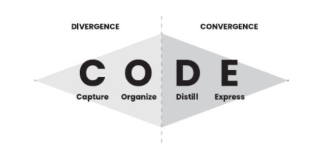 <small>Overlapping ideas of C.O.D.E. and divergence/convergence from Tiago Forte's book Building a Second Brain (Atria Books, 2022) </small>
Forte's focus on organizing is dedicated solely on to putting things into folders, which is a light touch way of indexing them. However it only indexes them on one axis—that of the folder into which they're being placed. This precludes them from being indexed on a variety of other axes from the start to other places where they might also be used in the future. His method requires more additional work and effort to revisit and re-arrange (move them into other folders) or index them later.
Most historical commonplacing and zettelkasten techniques place a heavier emphasis on indexing pieces as they're collected.
Commonplacing creates more work on the user between organizing and distilling because they're more dependent on their memory of the user or depending on the regular re-reading and revisiting of pieces one may have a memory of existence. Most commonplacing methods (particularly the older historic forms of collecting and excerpting sententiae) also doesn't focus or rely on one writing out their own ideas in larger form as one goes along, so generally here there is a larger amount of work at the expression stage.
Zettelkasten techniques as imagined by Luhmann and Ahrens smooth the process between organization and distillation by creating tacit links between ideas. This additional piece of the process makes distillation far easier because the linking work has been done along the way, so one only need edit out ideas that don't add to the overall argument or piece. All that remains is light editing.
Ahrens' instantiation of the method also focuses on writing out and summarizing other's ideas in one's own words for later convenient reuse. This idea is also seen in Bruce Ballenger's The Curious Researcher as a means of both sensemaking and reuse, though none of the organizational indexing or idea linking seem to be found there.
This also fits into the diamond shape that Forte provides as the height along the vertical can stand in as a proxy for the equivalent amount of work that is required during the overall process.
This shape could be reframed for a refined zettelkasten method as an indication of work
Forte's diamond shape provided gives a visual representation of the overall process of the divergence and convergence.
But what if we change that shape to indicate the amount of work that is required along the steps of the process?!
Here, we might expect the diamond to relatively accurately reflect the amounts of work along the path.
If this is the case, then what might the relative workload look like for a refined zettelkasten? First we'll need to move the express portion between capture and organize where it more naturally sits, at least in Ahren's instantiation of the method. While this does take a discrete small amount of work and time for the note taker, it pays off in the long run as one intends from the start to reuse this work. It also pays further dividends as it dramatically increases one's understanding of the material that is being collected, particularly when conjoined to the organization portion which actively links this knowledge into one's broader world view based on their notes. For the moment, we'll neglect the benefits of comparison of conjoined ideas which may reveal flaws in our thinking and reasoning or the benefits of new questions and ideas which may arise from this juxtaposition.
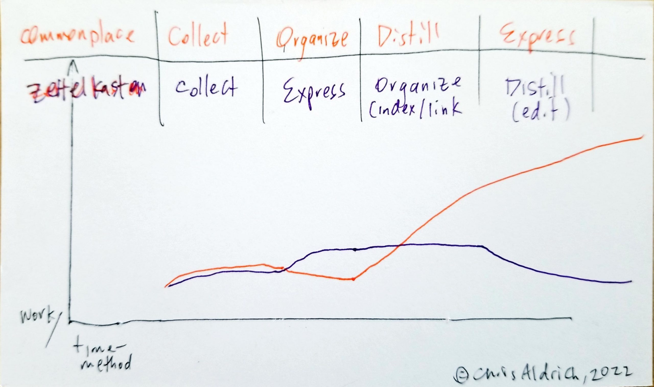
This sketch could be refined a bit, but overall it shows that frontloading the work has the effect of dramatically increasing the efficiency and productivity for a particular piece of work.
Note that when compounded over a lifetime's work, this diagram also neglects the productivity increase over being able to revisit old work and re-using it for multiple different types of work or projects where there is potential overlap, not to mention the combinatorial possibilities.
--
It could be useful to better and more carefully plot out the amounts of time, work/effort for these methods (based on practical experience) and then regraph the resulting power inputs against each other to come up with a better picture of the efficiency gains.
Is some of the reason that people are against zettelkasten methods that they don't see the immediate gains in return for the upfront work, and thus abandon the process? Is this a form of misinterpreted-effort hypothesis at work? It can also be compounded at not being able to see the compounding effects of the upfront work.
What does research indicate about how people are able to predict compounding effects over time in areas like money/finance? What might this indicate here? Humans definitely have issues seeing and reacting to probabilities in this same manner, so one might expect the same intellectual blindness based on system 1 vs. system 2.
Given that indexing things, especially digitally, requires so little work and effort upfront, it should be done at the time of collection.
I'll admit that it only took a moment to read this highlighted sentence and look at the related diagram, but the amount of material I was able to draw out of it by reframing it, thinking about it, having my own thoughts and ideas against it, and then innovating based upon it was incredibly fruitful in terms of better differentiating amongst a variety of note taking and sense making frameworks.
For me, this is a great example of what reading with a pen in hand, rephrasing, extending, and linking to other ideas can accomplish.
Tags
- visualizations
- writing
- commonplace books
- Tiago Forte
- misinterpreted-effort hypothesis
- writing for understanding
- compounding value
- behavioral economics
- knowledge work
- efficiency
- work
- C.O.D.E.
- cognitive bias
- imitation for innovation
- zettelkasten
- innovation
- time
- putting in the work
- commonplace books vs. zettelkasten
- productivity
- divergence/convergence
Annotators
-
-
www.w3schools.com www.w3schools.com
-
The else keyword in a for loop specifies a block of code to be executed when the loop is finished
This statement is as exact as useless. It doesn't explain the purpose of an else statement in a for loop. The example is even more confusing, because the result is exactly the same with the second print statement without the else.
-
-
www.facebook.com www.facebook.com
-
ĐÃ ĐẦU TƯ CỔ PHIẾU THÌ KHÔNG THỂ THIẾU PHÂN TÍCH CƠ BẢNĐọc tiêu đề bài viết này chắc chắn không ít bạn sẽ phản ứng ngay vì cho rằng bản thân mình và nhiều người khác vẫn kiếm bộn tiền từ đầu tư mà có cần gì cái gọi là phân tích cơ bản đâu. Tuy nhiên, cứ dành thời gian đọc hết quan điểm của mình và cùng nhau phản biện.Trước tiên, bài viết này sẽ loại bỏ những chiến lược đầu tư đặc biệt như đầu tư định lượng (Quantitative) hoặc giao dịch đối xứng (Hedging). Lý do là vì 2 phương pháp này đòi hỏi những kỹ thuật giao dịch rất khó, không phù hợp với số đông nhà đầu tư phổ thông. Phần nhiều chúng ta chỉ phù hợp với: Scalping (mua bán siêu ngắn đảo hàng liên tục trong 1-3 ngày), Swing (mua bán theo các con sóng kéo dài vài ngày đến vài tháng) hoặc Holding (mua và nắm giữ một thời gian dài theo câu chuyện của doanh nghiệp).Bạn giao dịch theo chiến lược nào trong 3 chiến lược trên? Thực ra thì chúng ta làm gì có quyền lựa chọn! Chính chiến lược sẽ lựa chọn chúng ta. Nó lựa chọn con người có bản chất và cá tính phù hợp với nó. Nhưng dù bạn lựa chọn theo hình thức nào thì bạn cũng phải sử dụng phân tích kỹ thuật, thông tin nội gián và phân tích cơ bản để bám theo hành động. Topic này, nhiệm vụ của mình là sẽ chứng minh cho bạn thấy nếu chỉ sử dụng mỗi phân tích kỹ thuật hoặc tin nội gián thì bạn rất rất khó để có thể gắn bó lâu dài với lĩnh vực đầu tư.Trước tiên là đối với phân tích kỹ thuật.Thế mạnh của phân tích kỹ thuật là cho chúng ta điểm mua bán một cách khá nhanh chóng và đơn giản. Tính hiệu quả của phân tích kỹ thuật thì rõ ràng đã được kiểm chứng qua thời gian. Nếu chúng ta kỷ luật theo đúng hệ thống đầu tư, quản trị tâm lý tốt thì thị trường muốn hạ gục chúng ta cũng khó. Tuy nhiên đó chỉ là ngắn hạn mà thôi, còn về dài hạn, thị trường nó có thể đo ván chúng ta một cách dễ dàng bởi những cú sụp đổ "trắng bên mua" với "nến gạch ngang" không thanh khoản trong cả 20-30 phiên, đến khi chúng ta có thể khớp được 1 lệnh bán thì giá đã mất 70-80% thị giá, ai dùng margin thì chắc chắn cháy tài khoản từ rất rất lâu rồi.Với những pha "đổ đèo kinh hoàng" như TTF (2008, 2016), JVC (2015), APC (2018), FLC ROS (2022), BII TGG (2016-2021),.... Thì dù chúng ta có giỏi phân tích kỹ thuật đến thế nào, kỷ luật cứng ra sao và tâm lý vững như bàn thạch thì cũng không thể tránh khỏi thua lỗ nặng lề.Vậy làm sao để tránh những "cái chết tang thương" như vậy? Mình chắc chắn tất cả những doanh nghiệp này, trước khi bị "đánh chìm" bởi những thông tin tiêu cực như gian lận báo cáo tài chính hay hành vi xấu của ban lãnh đạo bị phanh phui thì đều đã có những dấu hiệu rõ ràng trên báo cáo tài chính. Chỉ có điều chúng ta có đủ kiến thức và sự chăm chỉ để bóc tách hay không mà thôi. Phân tích cơ bản lúc này nó là "bức tường rào kiên cố" bảo vệ bạn khỏi những khoản đầu tư rủi ro.Nhiều bạn có thể nói mình là dân phân tích cơ bản thì làm sao hiểu hết phân tích kỹ thuật. Mình tự tin là mình đủ am hiểu để nói chuyện với mọi người về nó. Cá nhân mình từng dành trên 5 năm để nguyên cứu phân tích kỹ thuật, là admin của diễn đàn SRSC, diễn đàn số 1 về PTKT Việt Nam những năm 2010-2014. Số Code Metastock và Amibroker mình viết cũng cả ngàn code rồi ấy. Cá nhân mình cũng từng kiếm tiền bằng nghề viết Code System thuê. Nói chung là cầy bừa nhiều mình đúc rút ra rằng chẳng có hệ thống đầu tư nào đánh bại được thị trường cả, vậy nên chúng ta đừng mất công tìm. Bạn thấy trong vài chục các huyền thoại đầu tư trên thế giới, có được mấy người sử dụng thuần phân tích kỹ thuật mà trở thành huyền thoại?Vậy đầu tư theo thông tin nội gián thì sao?Hình thức này nếu bạn không có kiến thức cơ bản thì cũng giống như sử dụng thuần phân tích kỹ thuật mà thôi, rồi cũng 9 lần ăn và 1 lần mất là mất tất, của thiên rồi lại về với địa. Tại sao mình nói như vậy?Thứ nhất là nếu bạn không quen thân trực tiếp với ban lãnh đạo chóp bu của doanh nghiệp thì thường những tin tức bạn nhận được đều là thông tin đã qua tay hàng trăm ngàn người rồi. Ai cũng bảo "em chỉ nói mình anh mà thôi" nhưng rồi "cả thế giới này biết". Khổ cái là khi ai cũng biết thì làm sao kiếm được tiền.Thứ hai, nếu bạn có quen thân với chóp bu và họ bơm tin trực tiếp cho bạn thì cũng làm sao chắc chắn họ sẵn sàng gánh chịu rủi ro để cho bạn cơ hội ngon ăn, vấn đề không phải là cho 1 lần mà là cho nhiều nhiều lần mà không mong nhận lại? Trên đời ngoài bố mẹ và anh chị em trong gia đình, còn có người tốt với mình đến vậy sao? Đặc biệt là trong lĩnh vực mà đồng tiền đi liền khúc ruột như thị trường tài chính.Mình cứ tỉ dụ như có người tốt với mình thật vậy đi. Tin họ bơm cho mình là chuẩn đi. Rồi nếu mình không có kiến thức về tài chính, kiến thức về lĩnh vực đó thì mình làm sao đánh giá được tác động của thông tin đó đến con số kinh doanh của doanh nghiệp? Làm sao biết tin đó ra thì upside giá là bao nhiều? Upside đó có đủ hấp dẫn về định giá để dòng tiền nhảy vào càn quét và đẩy giá cổ phiếu đó lên cao? Có khi chưa chắc người bơm tin cho mình đã trả lời được những câu hỏi đó. Trong đầu tư có một "cái chết" lãng xẹt, đó là chết vì biết tin quá sớm và hành động sai thời điểm.Vậy nếu trong tình huống này chúng ta biết phân tích cơ bản thì sao? Thì chúng ta có thể nhanh chóng đánh giá được tác động của thông tin đó đến báo cáo tài chính, chúng ta có thể ước được điểm rơi của lợi nhuận và chúng ta có thể từ chối đi tiền nếu như upside không đủ hấp dẫn. Như vậy không tốt hơn sao?Nguồn gốc của một chu kỳ tăng giá cổ phiếu dài hơiĐầu tư sợ nhất là ôm cổ phiếu không có sóng hoặc sóng giảm. Lúc này phương án hay nhất là đứng ngoài, đánh đấm kiểu gì rồi cũng "ăn hành" hết, nhưng mấy ai đủ bản lĩnh để đứng ngoài?Sẽ tốt hơn rất nhiều nếu chúng ta chủ động phán đoán hoặc đi theo dòng chảy của tiền. Dòng tiền đổ về đâu thì tài sản của ta ở đó. Bơi xuôi dòng lúc nào chả ngon ăn hơn bơi ngược dòng, chỉ mất 20% sức mà thu về 80% thành quả.Hãy đi tìm những dòng cổ phiếu có xác xuất tăng giá dài hơi. Nguồn gốc của một cổ phiếu tăng giá mạnh mẽ trong thời gian dài hạn chính là có dòng tiền gia nhập. Nguồn gốc để dòng tiền gia nhập chính là "câu chuyện hấp dẫn". Và nguồn gốc của một câu chuyện hấp dẫn chính là những thay đổi lớn về mặt số liệu kinh doanh nội tại.Vậy làm sao để chúng ta có thể tìm được những câu chuyện hấp dẫn trước khi thị trường nhìn ra. Chỉ có 1 thứ thôi, đó chính là phân tích cơ bản. Nếu ví phân tích kỹ thuật là đèn Cos thì phân tích cơ bản như đèn Pha vậy. Nó sẽ giúp bạn nhìn thấy trước những thứ mà mấy ông bật Cos có mở to mắt cỡ nào cũng không nhìn ra được.Vậy làm sao để ứng dụng phân tích cơ bản trong việc tìm kiếm cơ hội đầu tư hấp dẫn? Bạn phải có 3 thứ: Thứ nhất là kiến thức nền tảng về phân tích cơ bản, Thứ hai là bộ công cụ giúp bạn nhìn nhanh được câu chuyện, và Thứ ba là cố gắng sắp xếp 2 tiếng đồng hồ để tham gia buổi Livestream của mình và Lê Thành (Trưởng bộ phận phân tích đầu tư của WiGroup), 2 đứa sẽ chia sẻ về kinh nghiệm của tụi mình trong việc "đãi cát tìm vàng", hứa hẹn không làm anh em thất vọng.Buổi Livestream được tổ chức vào 19h30 HÔM NAY, Chủ nhật, Ngày 27/02/2022 trên cộng đồng VWA - Cố vấn tài chính Việt Nam, có share về tường của mình và Fanpage WiGroup.Link đăng ký sự kiện: https://www.facebook.com/events/457936749448053 Bài viết này đã có quảng cáo, không có tiền thì ghõ phím làm sao ...- Thằng nghiện dữ liệu1K Chau Thien Truc Quynh, Thanh Tran and 1K others69 Comments166 SharesLikeShare
.
Tags
Annotators
URL
-
-
www.schneier.com www.schneier.com
-
To me, the problem isn’t that blockchain systems can be made slightly less awful than they are today. The problem is that they don’t do anything their proponents claim they do. In some very important ways, they’re not secure. They doesn’t replace trust with code; in fact, in many ways they are far less trustworthy than non-blockchain systems. They’re not decentralized, and their inevitable centralization is harmful because it’s largely emergent and ill-defined. They still have trusted intermediaries, often with more power and less oversight than non-blockchain systems. They still require governance. They still require regulation. (These things are what I wrote about here.) The problem with blockchain is that it’s not an improvement to any system—and often makes things worse.
Blockchain does not improve monetary systems
With cryptocurrencies—built on blockchain—we still need: centralization, trust, regulation, governance, and a whole host of other things that are already in TradFi.
-
-
www.youtube.com www.youtube.com
-
Diagrams as Code 2.0 • Simon Brown • GOTO 2021
"long-lived documentation" - "Think about diagrams as 'disposable' artifacts"
https://c4model.com/ C4 Model - model for visualizing software architecture; hierarchal dataset; Diagrams as abstractions, differing levels of technical details; think of it as zooming into maps at different levels * Level 1: Context * Level 2: Containers * Level 3: Components * Level 4: Code
Product Comparisions - Working with the DSL (Lite v. CLI v. DSL Editor): https://structurizr.com/help/dsl - Product offerings (Lite v. Cloud v. On-premise): https://structurizr.com/products
The DSL is rendering tool agnostic
Diagrams as code 1.0 - PlantUML, Mermaild, etc are input formats
Diagrams as code 2.0 - PlantUML, Mermaild, etc are output formats
Checkout: - Online REPL: https://structurizr.com/dsl?example=amazon-web-services - DSL Guidance: https://github.com/structurizr/dsl/tree/master/docs/cookbook - Examples: https://github.com/structurizr/examples
-
-
notebooksharing.space notebooksharing.spaceNotebook1
-
Add a marker for each station s = df.loc[df['Höhe [m]'] < 1000] ax.scatter(s['Länge [°E]'], s['Breite [°N]'], marker='o', color='C0', transform=ccrs.Geodetic(), s=40, edgecolors='k', linewidths=1, zorder=99, label='h < 1000 m a.s.l.');
Code duplication
-
-
www.biorxiv.org www.biorxiv.org
-
Note: This rebuttal was posted by the corresponding author to Review Commons. Content has not been altered except for formatting.
Learn more at Review Commons
Reply to the reviewers
Reviewer #1 (Evidence, reproducibility and clarity (Required)): **Summary:** Techniques to probe the local environment of membrane proteins are sparse, although the influence of lipids on the membrane protein's function are known since many years. Therefore, the paper by Umebayashi et al. is important. The environment-sensitive dye Nile red (NR) coupled to a membrane protein is an appropriate sensor for monitoring the local membrane fluidity. Linking of Nile red to the receptor via a flexible tether was achieved with the acyl carrier protein (ACP)-tag method. Experiments showed that depending on the ACP site a certain linker length is required to have NR inserted in the membrane and thus be an effective sensor for lipid disorder. This technology could be of general usability to study the environment of membrane proteins in the context of their function. As an example, the technique allowed insulin induced membrane disorder in the close insulin receptor vicinity to be observed. Further, results suggested that tyrosine activity is required for this disorder to happen. The experimental results appear to be complete and controls were made.
**Major comments:** 1) Sometimes technical terms are used without explanation: What is the GP value? What is ACP-IR? The spectrum was measured in number of rois? The reader can find those abbreveations out, but it would be nice to have them defined.
We have made a list of abbreviations.
2) Fig. 1d) is confusing. The ACP-IR labelling is evident in 3 panels, but there is no difference in the color (emission spectra of 1992-ACP-IR vs 2031-ACP-IR should be visible??). The DAPI staining is very different. When doing the latter, how difficult is it to get the staining equal?
The differences in spectra cannot be seen because we used pseudo colors for display of the DAPI and CoA-PEG-NR staining. The reviewer’s comments about the unequal DAPI staining is correct. The reason for this is most likely that the cell membrane is unequally permeabilized by PFA treatment. As the point of this figure is just to show that the plasma membrane is labeled, dependent upon the expression of the ACP-tagged insulin receptor, we don’t think that the variable intensities of the DAPI staining is important. DAPI is simply used to indicate the position of the cells.
3) How can one interpret Fig. 4: a) Control goes over 4 frames, at 240" insulin is added, and 10 frames should show a fluctuation difference?
We showed 4 frames after control treatment that showed no significant change was observed by control treatment. We expected that clear changes would be invoked by insulin treatment in GP images, however these changes, while visible in the GP images, are difficult to see for the untrained observer. This is the reason why we used the ZNCC method in the subsequent figures to better visualize the changes.
- b) A color shift from blue to green is visible after insulin addition. But it is faint - difficult to assess from the pseudo color scheme. What does 1000 pixel top/1000 pixel bottom mean in c). Is it an attempt to better visualize the fluctuation? It is difficult to recognize a difference before and after adding insulin. d) It seems that the kymograph set should show this. What is the color scale? Why is 3 so untypical, i.e., no change? Box 6 is also peculiar: the left side does not show a strong change upon insulin administration, the right side does. Why? We appreciate the helpful comments for improving our manuscript.
As pointed out, the change of GP value is extremely small before and after insulin addition, so it is difficult to fully visualize the change with normal pseudo-color expression. To deal with this, we adopted the following two methods to visualize minute changes.
1) Visualization of local changes of the statistical GP value showed by ZNCC throughout the time-lapse images (Fig. 6 and Fig. S2B).
2) Visualization of the top/bottom 1000 pixels of the sorting ZNCC value in each image (Fig. 7 and Fig. S2C). The top 1000 pixels are the ones that showed the largest changes. The bottom 1000 pixels are the ones that showed the smallest changes.
Owing to these expressions, we found out that the level of the response against the insulin signal was spatially and temporally heterogeneous in the membrane.
As for the color scale, in order to clarify the meaning of the difference of color, we have added the description about the relationship between the color and the ZNCC value in the results section.
4) How is the kymogram calculated? The legend says 'The horizontal dimension represents the averaged ZNCC inside the rectangular area, and the vertical dimension represents time'. The averaged ZNCC is a single value, so it is not clear why the kymogram shows a variation from left to right. May it be the ZNCC was averaged just vertically?
We apologize that we did not provide information regarding making the kymograph.
In the yellow rectangular area (Fig. 6B), the ZNCC values of the pixels with the same x coordinate value were vertically averaged, which were represented as the horizontal direction of the kymograph. That is, one horizontal line of the kymograph holds the spatial distribution of the ZNCC value along the horizontal direction of the membrane, and the vertical direction shows their time changes. To make it easier to understand, we refined the description about the kymograph in the legend of Fig. 6.
5) When calculating cross-correlation values on images, they need to be aligned. What fraction of the total image does the selected 19x19 box represent? As described, I imagine that a rolling CC over 19x19 pixels is calculated over an image from the time lapse series comparing it with the reference Iave(x,y). Compared to the 3x3 median filtered CP image, the ZNCC image should then be much more blurred??
Below we provide more information regarding the calculation of ZNCC.
Each local window for ZNCC calculation is set to a 19x19 pixels centered on every single pixel excluding the edges of an image. The ZNCC value calculated in that window is set to a center pixel of that area. After that, a new window centered on the adjacent pixel is set and calculate the new ZNCC. That is, the calculation window is slid throughout the image. Also, the calculated ZNCC value is not set to all the pixels of the window, but is set to only the center pixel of the window, so there is no blur effect like median filtering.
The figure below shows a schematic view of our ZNCC calculation.
Schematic view of our ZNCC calculation
**Minor comment:** On page 16 supplementary is not spelled properly.
corrected
Reviewer #1 (Significance (Required)):
The key point of this paper is convincing and the new technology appears to have a lot of potential. It can be applied to study membrane protein function in the context of its environment, the lipid bilayer.
Membrane fluidity measurements have been developed (e.g., using fluorescent probes like laurdan). However, the trick to link a probe like nile red by ACP technology to the insulin receptor and to observe its activity is quite new.
A most recent description of such a technology is in TrAC Trends in Analytical Chemistry Volume 133, December 2020, 116092.
This is an interesting review, but not directly impacting on our work.
**Referees cross-commenting**
All comments are constructive and important. The paper is important but needs to be amended as proposed.
Reviewer #2 (Evidence, reproducibility and clarity (Required)): **Summary:** In this manuscript, authors generated an ACP-attached Nile Red probe in order to specifically label Insulin receptor in the membrane. Owing to this specificity, one can measure the lipid membrane properties around a specific protein in the membrane. **Major comments:**
For the conclusions in the manuscript to be convincing, in my opinion, these additional data need to be added. Some of these are new experiments, and some are detailed analysis of existing data. The new experiments are not for new line of investigation, instead it is to confirm their statements and conclusions. The major point is the reliability of spectral shift. In usual environment sensitive probes, it is certain that they are in the membrane whatever is done to the membrane. However, when the probe is attached to a protein, it is not trivial to have the same confidence that the probe is always inside the membrane, and it is in the same plane of the membrane. 1992-ACP-IR is a good example; authors state that it binds to the protein outside the membrane, but when there is cholesterol addition and -maybe more interestingly- cholesterol removal, the dye still reacts and changes its emission (even PreCT changes its emission quite a bit at the 570 nm region). This is a clear indication of a change in localization of the probe upon some changes in the membrane. This implies that observed spectral shifts may not be due to lipid packing differences, but due to localization of the probes. For this reason, it is crucial to know where any environment sensitive probe localize in the membrane with respect to membrane normal, and this knowledge is more important for this probe. Related to this, the spectral difference upon insulin treatment and activation of insulin receptor could be due to changes in probe's localization in the membrane. Especially because authors show in Fig1e, the spectra can change depending on the probe localization. Relatedly, quantum yield of NR should be significantly different when it is inside vs outside membrane. Authors should show QY for 1992-ACP-NR and 2031-ACP-NR with different PEG lengths and upon insulin treatment.
We understand the logic of the request to measure the QY, since the QY of Nile red is much higher in organic solvents than in aqueous solutions, so it might be predicted that the QY of Nile red is higher in a lipid bilayer than when covalently bound to the protein in an aqueous environment. However, this argument depends upon the mechanism for the increase in quantum yield when going from aqueous to a non-polar solution. One possible explanation is based on the intrinsic properties of the dye under the two conditions. The alternative explanation would be that the dye would aggregate (be insoluble) in aqueous solution and therefore either not fluoresce or self-quench. In this case, we believe that the latter is the explanation because we and others have previously shown the turn-on properties of the probe when binding to proteins (SNAP-tag and others). It is not simple to measure QY in the cell under a microscope, but we have done something similar shown in supplementary figure 4. We labeled the three ACP-receptor complexes with PEG11-Nile red and co-stained with antibody to the Insulin Receptor. We then calculated a relative quantum yield. There were very little differences at all between the relative quantum yields, so we conclude that it is not the environment of the probe, which affects the quantum yield under these conditions, but the fact that it is covalently attached to a protein and incapable of forming aggregates. What distinguishes these constructs is the emission spectrum, not the quantum yield. In supplementary Table 2 we also did QY measurements in vitro and we could reproduce the increase of quantum yield by association with liposomes or in organic solvents. We tested whether non-covalent association with a protein would increase the QY by incubation with the lipid binding protein, BSA, in PBS. This was not the case, strongly pointing to the conclusion that it is the covalent association with the protein that increases the QY, not association with a protein. We believe that our demonstration of changes in fluorescent spectra with changes in cholesterol, large changes in fluorescent spectra with linker length for the 1992 construct and voltage sensitivity using patch-clamp prove that the Nile red is reporting on the membrane environment under the conditions we propose.
**Minor comments:** - Fig 1d requires quantification We do not agree on this. This is simply to show that the labeling is dependent upon expression of the relevant ACP-IR constructs. There is no detectable labeling of the control.
-
Voltage sensitivity of different PEG length of 2031-ACP probe should be added. We have added this data in figure 2 panel E.
-
Fig 3a graph should show all data points, not only bar graphs. Also, the band in 3a for +CoA-PEG-NR is dimmer than other bands, is it specific to this particular gel since quantification does not show any difference?
There is no significant difference- Fig 4d, colour code is needed.
Done
- Fig 5b and Fig3d are basically the same experiments in terms of control measurement, why is the difference in 3b is 0.04 GP unit while it is 0.007 GP unit?
We explain in the MS, but have improved the title of Y-axis in Fig.5 b graph so that the difference in what is plotted is clear. - Why is inhibitor data so noisy? We should discuss.
We don’t know the exact reason why inhibitor data is noisy, but we speculate that the actin cytoskeleton and phosphoinositide-dependent signaling could affect the membrane stability, and the membrane environment would be fluctuated in the presence of latrunculin B or PI3K inhibitor.
Reviewer #2 (Significance (Required)): Overall, this is a very useful approach, and this line of research will yield very useful tools to shed light on how lipids surrounding proteins can change their function. Major advance of the paper is the new chemical biology tool. There is also biological data on how insulin can change the insulin receptor's membrane environment which is contradictory to some old literature claiming that InsR becomes more "rafty" upon insulin treatment (e.g., PMID: 11751579).
If this type of tagging proves robust and reproducible (limitations and concerns listed above and below), it could be used by other researchers to tag their protein of interest and investigate the lipid environment around those proteins.
The downside of this method is that the probe requires ACP tag, a relatively less used tag than others in biology, therefore researchers interested in using this probe should have their proteins with ACP tag. Moreover, the linker length and ACP-tag position are quite crucial parameters (and probably should be optimized for each protein). Longer PEG lengths cannot report on changes efficiently (Fig3b), while shorter lengths are prone to artefacts as they can go out of membrane (Fig1 and Fig2). This might limit its widespread use.
The reason for using the ACP tag is that neither the SNAP tap nor the HALO tag working. The tethered Nile Red preferred to bind to the tqg rather than inserting into the membrane.
**Referees cross-commenting** I agree with all comments and concerns of other reviewers. I see the usability and potential of this new technology along with its limitations as all three reviewers pointed out.
Reviewer #3 (Evidence, reproducibility and clarity (Required)): See below. No concerns on any of these issues.
Reviewer #3 (Significance (Required)): **Critique:** This MS reports a proof-of-principle for using site-directed environmentally sensitive probe technology to assess the local membrane environment of a receptor tyrosine kinase (IR) upon activation. This technology addresses a major gap in our arsenal of tools to study the mechanisms of membrane signaling as the parameters of interest are biophysical parameters rather than purely biochemical ones. How to do this with spatial and temporal resolution is a major challenge. This study builds on previous work by the Riezman group that develops an extrinsic labeling system to tether Nile Red to specific sites on the ectodomain of a signaling receptor and then probe local membrane environments as a function of receptor activity. This is a carefully done study is well-controlled, is clever in design and is well-described. Although the major issues to which such a general technology could contribute involve intracellular (and not extracellular) event, the advances described will be of general interest -- particularly that local membrane order decreases when IR becomes activated. Specific comments for the authors' consideration follow:
**Specific Comments:** (i) As a general comment, the authors are measuring extracellular plasma membrane leaflet properties that may or may not translate to what is happening in the local inner leaflet environment. A general reader may well miss the significance of this. This point needs to be more explicitly emphasized in the Discussion.
This has been discussed in the revised version.
(ii) Why not treat cells with a PLC inhibitor to block PIP2 hydrolysis and ask if that inhibits membrane disorder. It is PIP2 hydrolysis/resynthesis that regulates the actin cytoskeleton at signaling receptors and this seems an attractive candidate for study.
There is a long list of attractive post-signaling events of the insulin receptor and how this works in different cell types that could be tested. We believe that this is beyond the scope of this study and we encourage others to do this.
(iii) The data acquisition time is at least 4 min which is long enough for activated receptors to be recruited to sites of endocytosis. Can the authors exclude the possibility that what they are measuring isn't reflective of such spatial reorganization? Does a clathrin inhibitor block the observed change in local membrane order for activated IR? We determined localization to AP2 adaptor containing clathrin coated pits at the cell surface and showed that during the time-course of the experiment that there is no significant change in co-localization or evidence for endocytosis (new figure 9). Therefore, we decided not to do the clathrin inhibitor blocking experiment because we believe that it could only lead to indirect effects.
(iv) Receptor activation is accompanied by other transitions such as dimerization, etc. Can the authors exclude the possibility that what they are measuring is related to changes in depth of insertion of the NR probe into the plasma membrane outer leaflet that is a consequence of IR conformational transitions associated with activation? This is highly unlikely given the fact that fluidification of the membrane environment is found with all length linkers. Given the intervals in increases in linker length on the 2031 construct, which is the closest to the membrane, it is very difficult to conceive that any of the ones larger than 5 PEGs restrict significantly the membrane insertion of the dye. **Referees cross-commenting**
I think we have a consensus opinion
-
Note: This preprint has been reviewed by subject experts for Review Commons. Content has not been altered except for formatting.
Learn more at Review Commons
Referee #2
Evidence, reproducibility and clarity
Summary:
In this manuscript, authors generated an ACP-attached Nile Red probe in order to specifically label Insulin receptor in the membrane. Owing to this specificity, one can measure the lipid membrane properties around a specific protein in the membrane.
Major comments:
For the conclusions in the manuscript to be convincing, in my opinion, these additional data need to be added. Some of these are new experiments, and some are detailed analysis of existing data. The new experiments are not for new line of investigation, instead it is to confirm their statements and conclusions. The major point is the reliability of spectral shift. In usual environment sensitive probes, it is certain that they are in the membrane whatever is done to the membrane. However, when the probe is attached to a protein, it is not trivial to have the same confidence that the probe is always inside the membrane, and it is in the same plane of the membrane. 1992-ACP-IR is a good example; authors state that it binds to the protein outside the membrane, but when there is cholesterol addition and -maybe more interestingly- cholesterol removal, the dye still reacts and changes its emission (even PreCT changes its emission quite a bit at the 570 nm region). This is a clear indication of a change in localization of the probe upon some changes in the membrane. This implies that observed spectral shifts may not be due to lipid packing differences, but due to localization of the probes. For this reason, it is crucial to know where any environment sensitive probe localize in the membrane with respect to membrane normal, and this knowledge is more important for this probe. Related to this, the spectral difference upon insulin treatment and activation of insulin receptor could be due to changes in probe's localization in the membrane. Especially because authors show in Fig1e, the spectra can change depending on the probe localization. Relatedly, quantum yield of NR should be significantly different when it is inside vs outside membrane. Authors should show QY for 1992-ACP-NR and 2031-ACP-NR with different PEG lengths and upon insulin treatment.
Minor comments:
- Fig 1d requires quantification
- Voltage sensitivity of different PEG length of 2031-ACP probe should be added.
- Fig 3a graph should show all data points, not only bar graphs. Also, the band in 3a for +CoA-PEG-NR is dimmer than other bands, is it specific to this particular gel since quantification does not show any difference?
- Fig 4d, colour code is needed.
- Fig 5b and Fig3d are basically the same experiments in terms of control measurement, why is the difference in 3b is 0.04 GP unit while it is 0.007 GP unit?
- Why is inhibitor data so noisy?
Significance
Overall, this is a very useful approach, and this line of research will yield very useful tools to shed light on how lipids surrounding proteins can change their function. Major advance of the paper is the new chemical biology tool. There is also biological data on how insulin can change the insulin receptor's membrane environment which is contradictory to some old literature claiming that InsR becomes more "rafty" upon insulin treatment (e.g., PMID: 11751579).
If this type of tagging proves robust and reproducible (limitations and concerns listed above and below), it could be used by other researchers to tag their protein of interest and investigate the lipid environment around those proteins.
The downside of this method is that the probe requires ACP tag, a relatively less used tag than others in biology, therefore researchers interested in using this probe should have their proteins with ACP tag. Moreover, the linker length and ACP-tag position are quite crucial parameters (and probably should be optimized for each protein). Longer PEG lengths cannot report on changes efficiently (Fig3b), while shorter lengths are prone to artefacts as they can go out of membrane (Fig1 and Fig2). This might limit its widespread use.
Referees cross-commenting
I agree with all comments and concerns of other reviewers. I see the usability and potential of this new technology along with its limitations as all three reviewers pointed out.
-
-
www.biorxiv.org www.biorxiv.org
-
Evaluation Summary:
This manuscript will interest a large community of molecular biologists studying translation and mRNA decay. The study provides a large-scale comparison of the roles of protein factors in No-Go Decay (NGD) and Codon-Optimality-Mediated Decay (COMD) in the yeast S. cerevisiae. A major strength of the manuscript is the direct comparison between one mRNA with a single strong translational stall and another similar mRNA with many slow translation sites (caused by changes in the genetic code). The analysis of both the factors that cause decay of these mRNAs as well as the ribosome states on the different mRNAs has the potential to reveal the molecular basis for the different mechanisms of mRNA quality control.
(This preprint has been reviewed by eLife. We include the public reviews from the reviewers here; the authors also receive private feedback with suggested changes to the manuscript. The reviewers remained anonymous to the authors.)
-
Reviewer #3 (Public Review):
The molecular basis for distinct mechanisms of mRNA quality control is poorly understood and an important problem in gene expression. In particular, the molecular mechanisms that act in response to a strong translation stall appear to differ from the mechanisms that act in response to continued slow translation. In this manuscript, a genetic screen revealed a quantitatively significant role for Syh1 in decay of an mRNA with a strong translation stall; similar effects of Syh1 on the same reporter had been reported in a 2020 publication from this laboratory. Here, they find that Syh1 function in mRNA decay does not require function of the major NGD regulator Hel2, of the NGD endonuclease Cue2 or of the ribosome disassociation factor Slh1. By contrast, none of these factors affect mRNA stability of a reporter in which translation elongation is likely uniformly slowed by suboptimal codons, but this reporter is a target of COMD (codon optimality mediated decay) and is stabilized by deletion of NOT5. The surprising result is that the strong stalling reporter is also regulated by Not5, in a manner quantitatively similar that of Syh1. Thus, mRNA stability of the strong stalling reporter is regulated by both NGD and COMD. To understand the molecular basis for recruitment of distinct decay factors, the authors investigate the ribosome states on these reporters using ribosome profiling. In the reporters without a strong stall site, single ribosomes and collided ribosomes are uniformly positioned across the coding sequence, while in the reporter with strong stall (due to CGA codons), ribosomes are absent from the region downstream of the CGA repeats and collided ribosome are substantially increased and stacked at the CGA repeat (compared to the OPT reporter). In addition, ribosomes lacking tRNA from the A site are enriched on the slowly translated reporter. The authors infer that the distinct ribosome signals of collided ribosomes or ribosomes with empty A sites are strong determinants of the factors that lead to mRNA decay.
A major strength of the manuscript is the direct comparison between one mRNA with a single strong translational stall and another similar mRNA with many slow translation sites (caused by changes in the genetic code). The analysis of both the factors that cause decay of these mRNAs as well as the ribosome states on the different mRNAs has the potential to reveal the molecular basis for the different mechanisms of mRNA quality control.
The genetic analysis is complicated and not completely consistent with the claim in the abstract that "Syh1 acts as the primary link to mRNA decay in NGD". While deletion of SYH1 does stabilize mRNA with a strong stalling site, the deletion of both SYH1 and genes encoding other factors known to be in the NGD pathway results in much greater stabilization of the mRNA with the strong stalling site. In the discussion, the authors correctly interpret this result as evidence of two independent mechanisms by which NGD is triggered. This is one of the most novel results presented in this manuscript, but is not followed up and leaves some questions about the primary role of Syh1 in NGD. Subsequent findings that neither Syh1 nor Hel2 are involved in decay of an mRNA encoded with non-optimal codons, that Not5 is involved in decay of mRNAs with non-optimal codons or strong stalls are convincing. The analysis of ribosome states on the same reporters in wild type and mutant strains provides clear and convincing differences in the ribosome states and distribution across the different reporters, which are likely to provide mechanistic insights into the distinct pathways. However, in the absence of any evidence of a causal relationship between these differences in ribosomal state and the difference in mRNA decay, the paper lacks sufficient support for the title "distinct ribosome states trigger diverse mRNA quality control pathways."
-
-
turingarchive.kings.cam.ac.uk turingarchive.kings.cam.ac.ukAMT-C-301
-
AMT/C/30
Annotation by Alan Turing. </br>Corrections, comments, and labeled code added to “the Prof’s book,” a report describing the methods Alan Turing and colleagues at Bletchley Park used to break the Enigma cipher. Turing was born on this day, June 23rd, in 1912. #Annotate22 174/365


-
-
www.biorxiv.org www.biorxiv.org
-
Reviewer #1 (Public Review):
In directed microbial evolution, separate populations of microbes are evolved in the laboratory and evaluated for their ability to exhibit one or more desirable properties. High-performing populations are then selected and subdivided into new populations, which are allowed to further evolve. This process is generally costly in both time and laboratory expenses, making it difficult to optimize the process, such as the type of selection that is employed. In contrast, evolutionary computation is a type of optimization where solutions to computational problems are evolved in silico, through imperfect reproduction of selected individual candidate solutions over multiple generations. Because evolutionary computation is much cheaper and faster that microbial evolution, there has been considerable research studying how different types of selection impact the evolutionary process. The goal of the current study is to see if selection mechanisms that have been shown to perform well in evolutionary computation experiments may also improve directed microbial evolution.
To date, microbial evolution experiments have used forms of truncation selection, where one or more of the "best" performing populations are selected for subdivision and further evolution. However, truncation selection, where some percent of the best performing individuals are selected, is known to result in rapid loss of diversity and poor performance in evolutionary computation. In this paper, the authors compare various types of individual selection methods from evolutionary computation to simulations of multi-objective microbial selection at the population level, where 22 distinct binary (pass/fail) objectives are evaluated and contribute to the fitness of a population in various ways. Specifically, they compare 5 selection methods: (1) elitism (where only the best population is selected); (2) truncation selection (where the top 10% of populations are selected); (3) tournament selection (in each of multiple tournaments, the best population of 4 random populations is selected); (4) lexicase multi-objective selection (where each of the objectives is evaluated sequentially, in a randomized order, and only those populations that can solve the current objective are retained and evaluated on the next objective); and (5) non-dominated multi-objective elitism (where any population that is not Pareto dominated by another population is selected). The first two of these are the methods commonly employed in directed microbial evolution, and the last three are simple versions of selection methods known to perform well in evolutionary computation. For controls, they also compare to random population selection and no selection (where all populations are retained).
The authors clearly explain the methods for simulating microbial evolution, how population fitness and diversity are evaluated, how the various forms of selection are implemented, and how results are compared through rigorous and appropriate statistical methods. The results are clearly displayed in informative graphs, which are also textually described to help the reader understand what the graphs are showing.
The results convincingly show that the multi-objective selection methods, in particular lexicase selection, out-perform the other selection and control methods tested in simulated directed microbial evolution of populations evolved to successfully perform multiple objectives. Although these results are not particularly surprising, they are an important demonstration that multi-objective selection mechanisms known to perform well in selecting individuals in evolutionary computation also work well when used to select populations of individuals in simulated microbial evolution, and may thus be strong candidates for helping to optimize evolutionary processes in real directed microbial evolution.
The authors candidly acknowledge limitations of the current study and describe future research that will address these limitations (e.g., using more sophisticated versions of the selection mechanisms tried here, and ultimately transferring successful methods to laboratory experiments of directed microbial evolution).
The paper is well-written and well-organized, including sufficient details for the reader to conceptually understand what was done, while including additional nitty-gritty details needed for reproducibility in the supplement and in open-source code.
This paper will be of interest to researchers working in directed microbial evolution as well as those in evolutionary computation. The authors compare various selection methods from the field of evolutionary computation to simulations of directed microbial population-level evolution. They convincingly demonstrate that multi-objective population-level selection outperforms the truncation selection of populations that is currently the norm in directed microbial evolution.
-
-
www.biorxiv.org www.biorxiv.org
-
Abstract
A version of this preprint has been published in the Open Access journal GigaScience (see paper https://doi.org/10.1093/gigascience/giy032 ), where the paper and peer reviews are published openly under a CC-BY 4.0 license.
These peer reviews were as follows:
Reviewer 1: Simone Romano
In this paper the authors describe and analyse a series of tools to find complex associations in large omics data sets. At the core of these tools lies the measure of association Maximal Information Coefficient (MIC) which recently received a lot of interest in data mining community. Other than presenting the first publicly available implementation of MIC to date, the authors make available the code for a complete pipeline to identify statistically significant associations between the features in a data set. This involves:- Computing the Total Information Coefficient (TIC) for each pair of features- Computing their p-value using a permutation test with Monte Carlo simulations- Select the significant pairs using statistical correction for multiple hypotheses- Rank the statistically significant associations according to MICMoreover, the authors analyse the results of their pipeline on synthetic and real data sets.I commend the authors for providing the community with a well-tested implementation of MIC (and its more recent version MIC_e) in various programming languages including C, Matlab, and Python. I also really appreciate publishing a full pipeline to identify associations between features written in Python, which is probably the most popular language in the data science community. Moreover, the paper is well written and the analyses about the effectivity of these tools are convincing. The paper should be accepted for publication in the GigaScience journal. There has been so much discussion about the merit of MIC in the past years since its publication in 2011. I am honestly impressed by MIC's authors efforts to shed light on the theoretical and empirical properties of MIC.
Their effort recently found venue in prestigious journals such as the Proceedings of the National Academy of Science (PNAS) in 2014, the Journal of Machine Learning Research (JMLR) in 2016, and the Annals Of Applied Statistics (AOAS) in 2017. The main criticism about MIC has been its similarity to one of the many estimators of mutual information. Even though MIC exploits mutual information, MIC has been shown to not be the same as estimating mutual information [Measuring dependence powerfully and equitably by Reshef et al. in JMLR 2016]. Nonetheless, what strikes me the most is that: in many empirical studies no estimator of mutual information has the same performance of MIC in terms of equitability. Being equitability a very intuitive property, I do understand why researchers and data mining practitioners value MIC.I have only one concern about the methodology of screening associations with TIC and ranking only the selected ones with MIC. Possibly if we are interested just in equitability, MIC should be the only association measure to be employed in the analysis. However, given than TIC shows to have more power the MIC [An Empirical Study of the Maximal and Total Information Coefficients and Leading Measures of Dependence by Reshef et al. in AOAS 2017], I guess that the associations that MIC would deem as significant would be a subset of the significant associations for TIC.Minor comments:- It would be great to describe the Storey's method to control the FDR in the paper to make it self-contained; It would be also great to briefly describe the procedure to control the FWER; - A table describing the difference between the data sets SD1 and SD2 would be informative. Possibly a line describing the Madelon semi-synthetic data sets would be useful too;-
The authors discuss a great insight on MIC when they say that: "associations between informative/redundant and redundant/redundant variables were significant also for a lower number of samples". It would be nice to have a visual example about these type of associations;- Figure 4 b. I guess discussing a decreasing FN is the same as discussing increasing power. Changing the FN plot in a power plot would make the paper more coherent: e.g. as in Figure 2 a;- "coniugate" in the abstract -> conjugate. Maybe better to reformulate this sentence as it is not very clear; Simone Romano
-
-
www.biorxiv.org www.biorxiv.org
-
Image
Reviewer 2: Christian Fournier
Reviewer Comments to Author, version 1: The authors investigate the ability of deriving plant biomass (both fresh and dry mass) from 2D image-based features acquired with visible, fluorescent and NIR multi-view imaging systems operating on an automated high throughput phenotyping platform. In a first part, several multivariate statistical models are compared for their ability at predicting biomass for two treatments within a single experiment, on three independent datasets, detailed results being presented for one experiment. One of the best model, the random forest, is then further investigated for its capacity at making prediction across experiments, being trained on one experiment at a time or on one treatment of one experiment at a time. Finally, the relative importance of individual image-based traits in the prediction of either fresh or dry weight is presented for two treatments of one dataset.
Models and methods for model evaluation are clearly presented, and the overall quality of the text and Figure makes the paper easy to follow. The inclusion of other than visible images, the objective selection of image-based traits, the comparison of models and the use of 3 independent datasets clearly distinguish this paper from previous publications on the same subject. It provides the reader very valuable information on the current prediction capacity of the approach, together with a consistent methodology for analyzing other related practices.
However, I have two major concerns on the current version of this manuscript.
First, I think that some conclusions highlighted in the abstract or in the text are not completely in line (or at least sufficiently tempered) with what is demonstrated in the text or shown on the figures. In the abstract (line 19-20), it is highlighted that 'The results proved that plant biomass can be accurately predicted from image-based parameters using a random forest model'. To me this conclusion is clearly supported by data in the case of within experiment predictions, but not fully in the case of the cross experiment test (i.e. quite opposite to what is stressed line 21). My impression, given results presented Figure 5, is that in one case out of two, a model trained on one experiment alone could not accurately (or at least with not the same accuracy) predict the biomass, despite a repeated protocol. This result is per se very interesting, as it demonstrates an important limitation of the approach. It can however not be summarized by what is written line 19-21, 201-202, 209-210 or 253-257. On another occasion (line 148 and line 248), I found the conclusion ('the RF model largely outperformed other models') a bit exaggerated, as, on Figure 3, depending on the criteria, RF model performs very similar to MARS model for example.
Second, I did not manage to test the models, nor to reproduce the analysis with the provided data and source code. Concerning the data, image traits are provided for all experiments, but manual measurement on Dry Weight are missing. Concerning the code, the R-script provided does not fit to the provided dataset, thus making it difficult to test. More important, model code runs with errors at runtime ('not defined' errors). I also think, but this is only a suggestion, that, in addition to raw image files, providing binary masks of plants, that are of high importance for all traits analyzed here, could improve the re-use of this nice dataset,.
Other minor points or comments for specific parts of the texts are provided bellow:
Line 72-74: I think this sentence would be better be placed in the Potential application section Line 85: Do you mean that some image traits are more sensitive to physiological traits ? I do not see why Fig 1B is illustrative for this point. Line 98: In the context of phenotyping, it might also be useful to add Spearman rank correlation to the assessment Line 108: Fig 1B is only a heatmap image. May be a list of traits should be provided, or a reference to the supplementary data should be added here. Line 117: Figure 2B is poorly informative as traits are not identified. This figure is also not commented in the text, I suggest removing it. Line 144: I would find useful to make here perfectly clear that all the models were trained on the control + stress plants, to avoid any confusion with the 'cross treatment test' later on (Figure 6) Line 146-151: I found the analysis a bit confusing as, in the details, the ranking of the different methods varies, and I do not clearly see why RF 'largely outperforms' other methods (especially MARS). Line 152-155: The comparison with the widely used 'single feature' method is very interesting. Can you consider to add its score/line on the R2 and RMSRE ? Line 178: May be it is also worth noting in the text that geometric + color traits trust 13 out of 15 (FW) and 15 out of 15 (DW) first places, as these two types of data are widely available among phenotyping platform and yet not so often used in biomass predictions. Line 201 - 211: The text seems to me a bit too optimistic regarding the cross experiment predictions. Exp3 clearly shows a non-conservation of the relationship obtained in Exp1 or 2, and a clear loss of predictive power compared to within experiment training. Line 281: typo: sophisticated Line 349: could you give an idea of the amount of such filled missing values? Line 400: the formulation is a bit strange as it sounds like a conclusion already. Line 426: DW data are missing. Line 535: legend of figure 5 did not really apply to these figures. A complete legend should be added.
Re-review:
I thank the authors for the work done on the new manuscript and on Github, that address most of the concerns I raised in my first review.
The pipeline published on GitHub now works nicely and allows to reproduces the different analyses. I only had to install manually two packages (earth and e1071). They could be easily added to the list of dependency in the R script to completely automatize the installation. The authors also clarify their analysis of the comparison of models, and the overstatement concerning the RF model has been corrected.
I however still think that the abstract should be amended to better match the conclusions of the cross experiment test. The author acknowledged, in their response and in the text (line 226) that one cross experiment test leads to a loss of predictive accuracy.
It seems also obvious, from Figure 5, and this should probably be added to the text, that this loss of accuracy is not linked to a greater random dispersion of the points, but to a systematic model bias. I agree with the authors that this may be due to some changes in the experimental conditions. My point is that these changes are not completely captured by the model, even with the inclusion of non structural traits. I therefore still think that there is some overstatement/ambiguity in the abstract, in particular in the sentence' The high prediction accuracy based on this model, in particular the cross experiment performance, will contribute to relieve the phenotyping bottleneck in biomass measurement in breeding applications' . This may however be easily fixed.
-
Abstract
This paper has been published under an Open Access CC-BY 4.0 license in the journal GigaScience, which includes Open Peer Reviews published under the same license. These are as follows:
Reviewer 1: Malia Gehan
Reviewer Comments to Author, version 1: Image datasets are available and are a valuable community resources. The code is available, which is great. While I definitely appreciate the authors work, I don't think the data support some of the statement throughout the paper, especially when it comes to the wording regarding MLR vs other models, unless further clarification can be provided (Figure 3). In some of the conditions (stress for example) MLR looks better than the other models. The inclusion of color, NIR, and Fluor traits into models is interesting.
Lines 14-15: I think this statement needs to be qualified by saying that it is a challenge to find a predictive biomass model across experiments, not that it is a challenge to find a biomass model 'in the context of high-throughput phenotyping', which is vague and I don't think accurate without further clarification considering the number of previous papers that model biomass from images with high correlation to ground truth measurements.
Lines 34 to 40: lacking in citations of literature. Introduction in general needs improvement in terms of the previous literature that it cites.
The second paragraph of the intro is a very limited short review of the literature but there are a number of papers that model biomass using ht-phenotyping that are not represented including Yang et al 2014 (nature communications), Montest et al. 2011 (Field Crops Research), Fahlgren et al. 2015 (Molecular Plant) to name a few.
Line 45: "On the other hand, to produce reliable assessments, suitable model types needs to be established and model construction requires integration of many components such as efficient mathematical analysis and representative data." Very vague.
Line 58: Please clarify this statement: "Another concern is that the number of traits used in these studies were quite limited and perhaps not representative enough. Therefore, a more effective and powerful model is needed to overcome these limitations and to allow better utilization of the image-based plant features which are obtained from non-invasive phenotyping approaches." Not sure what this means exactly, very vague considering that the papers mentioned do have models of biomass that are not 'perfect' but do have high heritability and correlation with ground truth measurements.
I think the authors need to adjust the justification of their research to stress that there needs to be biomass models that can be used across experiments/environment/treatments, which they do say, but needs to be stated more clearly. In general, many of the justification statements, which are pointed out in points 3 and 4 above are obscure to the point that they lose meaning.
Line 146 : "Although the performance of these models was roughly similar, RF, SVR and MARS methods had better performance than the MLR method for prediction of both FW (Fig. 3B) and DW (Fig. 3D), implying a nonlinear relationship between image-based phenotypic profiles and biomass output." This doesn't seem accurate, it looks like MLR has just as good predictive power in many of the situations presented. I don't think you can say that MLR and the others are roughly similar and then say that this implies a nonlinear relationship. Can this conclusion be clarified? It seems like there are only small differences between the models.
Regardless of whether or not random forest is the 'best' model, the data doesn't seem to support the statement that the RF model 'largely' outperformed the other models. This only seems accurate under the control condition, can this be clarified?
Line 238: "Although previous attempts have been made to estimate plant biomass from image data, most of these studies consider only a single image-based feature or very few features in their models which are often linear-based, ignoring the fact that the phenotypic components underlying biomass accumulation are presumably complex. Accurately predicting biomass from image data requires efficient mathematical models as well as representative image-derived features." I disagree with the authors on this point, if biomass can be modeled with a few features with high correlation why does it matter if they presume that it is complex? Their more complex models were still decreased in R2 with environmental differences and between experiments and I don't find the data suggesting that RF model outperforming other models (particularly MLR) convincing without further clarification.
Re-review: Chen et al, appear to have addressed each reviewer comment, below are some minor language changes for the revised sections.
Minor changes (language changes) 1. Line 47: remove "some other traits" seems unnecessary 2. Line 64: change "they" to Buesmeyer et al. 2013, and change "make it a question" to "question" 3. Line 73 change besides to "Further" 4. Line 75 change to "due to a lack of datasets for assessment"
-
-
www.econometrics-with-r.org www.econometrics-with-r.org
-
# import data on the Wilshire 5000 index W5000 <- read.csv2("data/Wilshire5000.csv", stringsAsFactors = F, header = T, sep = ",", na.strings = ".") # transform the columns W5000$DATE <- as.Date(W5000$DATE) W5000$WILL5000INDFC <- as.numeric(W5000$WILL5000INDFC) # remove NAs W5000 <- na.omit(W5000) # compute daily percentage changes W5000_PC <- data.frame("Date" = W5000$DATE, "Value" = as.numeric(Delt(W5000$WILL5000INDFC) * 100)) W5000_PC <- na.omit(W5000_PC)
I prefer to run a simpler code here:
       library(pdfetch)
       library(quantmod)

       W5000  = pdfetch_FRED("WILL5000INDFC")                      # fetch the data directly from the FRED database as an "xts" and "zoo" object
 names(W5000) = "W5000"                                            # the date format is "YYYY-MM-DD"

       W5000    = na.omit(  W5000["1989-12-29::2013-12-31"]  )     # subset the sample from 29 Dec 1989 to 31 Dec 2013, and remove the NAs
       W5000_PC = na.omit(  Delt(W5000)*100                  )     # compute the daily percentage changes, and remove the NAs
-
-
activeviam.com activeviam.com
-
```javaCopperStore rateStore = Copper.store("Rates").joinToCube().withMapping("Base cur.", "Currency"); ```
The Java code marker has pop-out
-
-
www.javatpoint.com www.javatpoint.com
-
Difference between Map and HashMap The Map is an interface in Java used to map the key-pair values. It is used to insert, update, remove the elements. Whereas the HashMap is a class of Java collection framework. The Map interface can only be used with an implementing class. It allows to store the values in key-pair combination; it does not allow duplicate keys; however, we can store the duplicate values. Its implementing classes are as follows: HashMap Hashtable TreeMap ConcurrentHashMap LinkedHashMap HashMap is a powerful data structure in Java used to store the key-pair values. It maps a value by its associated key. It allows us to store the null values and null keys. It is a non-synchronized class of Java collection.
Tags
Annotators
URL
-
-
openclassrooms.com openclassrooms.com
-
Vous connaissez maintenant la différence entre conteneur et machine virtuelle ; vous avez ainsi pu voir les différences entre la virtualisation lourde et la virtualisation légère.Un conteneur doit être léger, il ne faut pas ajouter de contenu superflu dans celui-ci afin de le démarrer rapidement, mais il apporte une isolation moindre. À contrario, les machines virtuelles offrent une très bonne isolation, mais elle sont globalement plus lentes et bien plus lourdes.
-
-
www.pythoncentral.io www.pythoncentral.io
-
Definition of Tuple in Python.
-
-
bafkreid7fzg5f6jb7rugtsu2lu33hzkvs4xfaoxzr5b75swqzandabzije.ipfs.dweb.link bafkreid7fzg5f6jb7rugtsu2lu33hzkvs4xfaoxzr5b75swqzandabzije.ipfs.dweb.link
-
forward-compatible applicationupdates
!- concept : forward-compatible application updates
- concept : forward-compatible applications
- permanent storage of data along with the code used to create processes it
- concept : forward-compatible applications
-
-
en.itpedia.nl en.itpedia.nl
-
Black Box testing: Software on the rack
Black Box testing: Software on the rack
Black Box testing is defined as a testing technique in which the functionality of an application is tested without looking at the internal code structure, implementation details and knowledge of internal paths of the software. This type of testing is completely based on software requirements and specifications.

-
-
arxiv.org arxiv.org
-
Applying Transformation. Assume a set of transformationrules Φ = {𝜙1, 𝜙2, 𝜙3, ...}. Given original code 𝑐𝑖 , 𝜙 𝑗 (𝑐𝑖 ) transformsthe code, changing the structure while preserving semantics. Fig-ure 3 shows how to apply such transformation to 𝑐𝑖 . It works inthree steps:• Find Transformation Location. Given a piece of source code (𝑐𝑖 ),we first use tree-sitter3 to parse out the AST (𝑇𝑐𝑖 ). From theAST, we extract potential locations for de-naturalization. Theselocations are nodes (𝑛𝑘 ) in 𝑇𝑐𝑖 . While choosing location 𝑛𝑘 from𝑇𝑐𝑖 , we consult Φ – we extract the nodes where at least one of𝜙 𝑗 ∈ Φ is applicable.• Select Transformation Rule. Once we have a set of such nodes,we filter out the transformation rules that cannot be appliedto any node of in 𝑇𝑐𝑖 . After such a filtration, we have a set oftransformations Φ𝑎 ⊆ Φ. At this stage, we randomly select onetransformation pattern 𝜙 𝑗 ∈ Φ𝑎 to apply at an application loca-tion (AST node) 𝑛𝑘 .• Apply Transformation. We apply 𝜙 𝑗 to 𝑛𝑘 to get the transformednode 𝑛′𝑘 . We then structurally match 𝑛′𝑘 with the original AST𝑇𝑐𝑖 , specifically 𝑛𝑘 . We adapt the context of 𝑛𝑘 to the transformednode’s (𝑛′𝑘 ) context. In that way, we get the transformed AST(𝑇 ′𝑐𝑖 ), which we then translate to get the transformed code 𝑐 ′𝑖 .We designed the transformation function 𝜙 𝑗 and subsequentcontext adaptation in such a way that preserves the meaning orfunctionality of the original code. We use AST analysis and (ap-proximated) data flow analysis on code AST
SPT的应用表述
-
-
wiki.c2.com wiki.c2.com
-
YouArentGonnaNeedIt (often abbreviated YAGNI, or YagNi on this wiki) is an ExtremeProgramming practice which states: "Always implement things when you actually need them, never when you just foresee that you need them."
Only implement features in code when you actually need them. Never implement features that you anticipate needing, because you aren't gonna need it (YAGNI).
Tags
Annotators
URL
-
-
www.econometrics-with-r.org www.econometrics-with-r.org
-
# set the column names colnames(USMacroSWQ) <- c("Date", "GDPC96", "JAPAN_IP", "PCECTPI", "GS10", "GS1", "TB3MS", "UNRATE", "EXUSUK", "CPIAUCSL") # format the date column USMacroSWQ$Date <- as.yearqtr(USMacroSWQ$Date, format = "%Y:0%q")
These lines of code are not necessary at all.
Simplified code:
                 USMacroSWQ <- read_xlsx("us_macro_quarterly.xlsx")

                        GDP <- ts( USMacroSWQ$GDPC96,                    start = c(1957, 1), end = c(2013, 4), frequency = 4 )      # define GDP as ts object
                  GDPGrowth <- ts( 400*log(GDP[-1]/GDP[-length(GDP)]),   start = c(1957, 2), end = c(2013, 4), frequency = 4 )      # define GDP growth as a ts object
                      TB3MS <- ts( USMacroSWQ$TB3MS,                     start = c(1957, 1), end = c(2013, 4), frequency = 4 )      # 3-months Treasury bill interest rate as a 'ts' object
                     TB10YS <- ts( USMacroSWQ$GS10,                      start = c(1957, 1), end = c(2013, 4), frequency = 4 )      # 10-years Treasury bonds interest rate as a 'ts' object

                    TSpread <- TB10YS - TB3MS                                                                                       # generate the term spread series
-
-
www.gobletqa.com www.gobletqa.com
-
Wildcard
Within code a wildcard is most commonly referenced via the * character
-
Test-First -
While Test-First is generally agreed upon to be better. It does have down sides One major downside is if ( or when ) requirements change The tests must be re-written around those requirements. Which means if the requirements are not clearly defined a lot of time is spent writing; then rewriting tests before any code has actually been written.
So Test-First is most beneficial when the requirements are clearly defined and not likely to change
-
addition of new code
It's more than just addition of new code. Its any change to the code base.
It could be the code was deployed to a new environment, but nothing else was change. Regression Tests help to ensure the code is running correctly in the new environment. For example promotion from a staging environment to production
-
with minimal instructions
While minimal instructions is always nice, it's not always the core goal of a refactor. Often time code refactor is done to improve clarity of its intent rather than minimize the amount written. The two often fall hand in hand, but that is not always the case. Many time improving clarity means the number of lines of code increases, which is not always a bad thing.
That said, it's a constant juggling act to between the two. You want code that is easy to understand and you want as little of it as possible. Which is a very difficult thing to accomplish.
It's often said a good developer writes code thats easy to understand and maintain. A great developer does the same, but with less code.
-
Cucumber
Let's not give out free advertising. Cucumber is software that contains a Gherkin parser. The parser is used to convert the feature file into an AST ( abstract-syntax-tree ) that other code can then use.
We use a custom parser called Parkin which has no relationship to Cucumber in anyway
All that said, I would change this to
Keywords indicate to the Gherkin parser what should...
-
