A bit of a pedantic turn, but sure...

As a girl, I had always noticed this. I would oftentimes hang out with my male cousins, who would love to play video games, and when I wanted the chance to play my grandmother would retort with claims that video games werent for girls, and that I should be playing with dolls instead. Even when I was older and I had the ability to access the internet on my own, the games online for girls were always catered towards beauty or princesses, there was never anything of substance made for girls as there were for boys. Video games have had a long history of doing so, as when they were first being developed, many game developers would struggle to create games catered for girls, unlike the shooter and fighting games meant for boys. Thankfully, over the years game developers have truly begun to understand what types of games women really want, and are continuing to build and innovate each year.

I found this reading very interesting because it shows how the social perception of programming has changed over time. In the early days, programming was considered less important work and was often done by women, even though many of them made significant contributions to the field. As software became more profitable and respected, the field gradually became more male-dominated. This made me realize that the status of a profession is not always based on the difficulty or importance of the work, but can also be shaped by social and economic factors. It also highlights why it is important to make technology fields more inclusive so that opportunities in influential and well-paid careers are accessible to everyone.

This is an aspect that I feel is underdeveloped. An idea I had recently was to have a "Station Day" once every so often (probably every month). On this day, students would go through stations with small group or individual games that were from their class's playground bucket. These games would be self led through diagram/directional pages but they could ask the teacher for assistance. Once they learn the game, their class would gain the pages for their bucket. I think this would allow students a better idea of what to do when they are outside, even if only for one recess. This could also reenforce the concept of being a "good winner" or "good sport" and being a team player outside of gym class.

Males are vulnerable, males are targeted.

That was a lot of verbiage for little gain by the reader. This is really a techno-cultural intelligencia fight by the "rationalists" bubble. Who really cares about this and what truly is the impact? It's similar to the Charlie Kirk phenomena - a seemingly large internet bubble (hmmm....2M world-wide followers - mostly in the US out of 330M people). Young and old of everyone I asked - no one had heard of him before his death. Maybe that's just my bubble - but using the "rationalists" approach - I think the data would play out - these bubbles are just not that big - they only feel that way when you're online.

Topics learned today - Grey Tribe (ugh), media vs hippies still exists

my girl oh my TT

这种是特定品类的实景流派

这类强叙事的游戏更多的体验是美术资产决定的

这里是一种经验范围的比例

走廊的最经典游戏

其实我实际过程中也赞成这一点，大概规划一下直接搭白盒就行了，因为3d游戏空间感更重要而且白盒搭起来挺快的比画画快多了。。

这种就是类似 冰与火的韦斯特罗大陆，或者类似指环王dnd的世界地图设定。相当于一个世界观的概念。

除非是纯文字游戏，否则游戏的剧情还是要对玩法和机制服务的，其实就是边做边圆剧情的感觉

一种感性的对关卡难度或者体验强度的规划

其实我理解就是把一些关键的东西（剧情情节，关卡机制，谜题设计等）先整理枚举好，然后按照一条特定的主轴节奏排布上去

其实这里的定位就是类似地心1的通关cg，这里先不做了，因为赶鸭是一个弱剧情的游戏。

赶鸭中目前缺少类似的设计，但是目前可以在每关的结尾处进行补充？

这里是踩坑的点和后续需要优化的点 需要制作一个游乐场测试场景对各类机制进行测试 1.一些物体的基础长宽高比例 2.一些关卡物体的机制和尺寸和玩家与鸭群的适配性

在第一次小組討論中，談及人物形象的時候，組員提及了荊軻是一個喜好和平和情緒穩定的人。但我不認同，我認為荊軻受到他人斥責時是有生氣的，但他選擇離開是因為他不希望把情緒爆發出來，原因不是因為喜愛和平，而是作為一個君子、讀書人，不應該隨便呈匹夫之勇。另一方面，刺客列傳中記載了荆軻出發刺秦王前，對太子丹的斥責十分嚴厲，而且他因為知遇之恩答應太子丹刺殺秦王也凸顯了他不是一位喜好和平的人，他沒有勸諫太子以和平的方式解決秦王的問題。

High school GPA and college coursework are better indicators because they represent a student's ability/willingness to do work. Standardized tests examine a student's ability to play "the game."

Social media is often seen as a "free range" for users to harass other users, with the idea that because all the information they found on the person is online, there's nothing objectively bad about publicising that information. There is also the matter of users often being behind anonymous accounts, where they're able to share this information without fear of retaliation. When users feel that someone has done something wrong, they often take things way too far. I've witnessed a situation where a woman was at a baseball game and a random person in the background made a disgusted face at the woman, and many of the users presumed that she did this with racist implications, as the person who was filming was a person of color. Users online then began to find the stranger's information- their house, job, linkedin, etc. They began to write fraudulent bad reviews under the stranger's job's review section, and eventually got the woman fired. This is just one of few cases of people on the internet taking things absolutely way too far, and causing greater harm to the stranger and the stranger's family, when people weren't even entirely sure if what she did was actially racist, or even deserved that type of behavior.**

Author response:

The following is the authors’ response to the original reviews

Public Reviews:

Reviewer #1 (Public review):

(1) The authors appear to be excluding a significant fraction of the TCRlow gamma delta T cells from their analysis in Figure 1A. Since this population is generally enriched in CD25+ gamma delta T cells, this gating strategy could significantly impact their analysis due to the exclusion of progenitor gamma delta T cell populations.

We were cautious in our gating strategy since the TCR𝛿+ CD3e+ subset is rather small and so low signal/background noise ratio can be an issue if the gates used are too broad/generous. There is some inevitable low level background staining with the TCR𝛿 that sits just above the bulk of the negative population and is CD3ε -ve. Although this background represents a tiny fraction of total cells, we were wary of gate contamination into our TCR𝛿+ CD3e⁺ subset and we wanted a gating strategy that could be applied across other organs too. We do not, however, believe this conservative strategy is impacting on measurements progenitor numbers across strains or our conclusions, since the size of this progenitor population in the various IKKΔT^CD2 and Casp8ΔT^CD2 strains was never impacted by the mutations. But to reassure the reviewer, we show our conservative gate as compared with a very broad TCR𝛿 gate and see we are not missing a substantial population of CD25+ cells just below our gate. This also helps illustrate how close the background from the CD27^int expressing αβ thymocytes (right column) comes to the TCR𝛿+ CD3+ gate and the importance of tight lineage gating.

Author response image 1.

(2) The overall phenotype of the IKKDeltaTCd2 mice is not described in any great detail. For example, it is not clear if these mice possess altered thymocyte or peripheral T cell populations beyond that of gamma delta T cells.

Given that gamma delta T cell development has been demonstrated to be influenced by gamma delta T cells (i.e, trans-conditioning), this information could have aided in the interpretation of the data.

Apologies for not being clearer on this point. We have studied conventional αβ T cell development in these strains in considerable detail, and these studies are published and discussed in some detail in the introduction in paragraph 3 on page 3-4 and in cited references Schmidt-Supprian et al 2004, SIlva et al 2014, Xing et al 2016, Webb et al 2019, Carty et al 2023. These detail how IKK expression is critical for thymic development of αβ T cells and their peripheral survival, and dissects the role of NF-κB activation and cell death regulation by IKK. However, we now add new discussion (page 11-12) that considers the potential impact of altered αβ T cell development in the strains used for this study.

We agree that trans-conditioning is also an important consideration, since CD4 TH17 T cells can enhance type 17 𝛾𝛿 T cell development (10.1038/icb.2011.50). This is of relevance to the limited conclusions we draw concerning type 17 𝛾𝛿 T cells. The REL and IKK deficient strains do lack effector populations, including type 17 αβ T cells, so it is possible that the absence of type 17 αβ T cells in these strains does contribute to the modest impact of IKK deletion in the type 17 𝛾𝛿 subset. We now highlight this information and discuss in the manuscript (page 11-12).

Related to this, it would have been helpful if the authors provided a comparison of the frequencies of each of the relevant subsets, in addition to the numbers.

We now provide both the absolute frequencies of different 𝛾𝛿 subsets and their relative frequencies to one another, as supplementary figure 2. We still believe assessing absolute numbers is the gold standard, since the differential impact of gene deletions on the αβ T cell compartments in different strains will effect whether or not αβ T cells are present, and therefore overall representation of 𝛾𝛿 T cells can vary considerably between strains. Hence, absolute numbers are more reliable measure of cell abundance.

(3) The manner in which the peripheral gamma delta T cell compartment was analyzed is somewhat unclear. The authors appear to have assessed both spleen and lymph node separately. The authors show representative data from only one of these organs (usually the lymph node) and show one analysis of peripheral gamma delta T cell numbers, where they appear to have summed up the individual spleen and lymph node gamma delta T cell counts. Since gamma deltaT17 and gamma deltaT1 are distributed somewhat differently in these compartments (lymph node is enriched in gamma deltaT17, while spleen is enriched in gamma deltaT1), combining these data does not seem warranted. The authors should have provided representative plots for both organs and calculated and analyzed the gamma delta T cell numbers for both organs separately in each of these analyses.

We did of course process and calculate numbers of different subsets in both lymph nodes and spleen. Where we saw loss of peripheral 𝛾𝛿 subsets, or rescue, this was reflected in seperate analysis of both organs and we did not see any organs specific effects in the mouse strains analysed. We therefore took the initial view that presenting aggregate data was most efficient and least repetitive representation of data. However, we very much recognise the reviewers concern, and interest to see these data, so have now included representative plots across both organs for figure 1D, and show cell numbers of lymph nodes and spleen separately, as well as together, for figures 1, 2, 4 and 7, and these plots reflect the differences observed when we combined data. We did not break down the data for all figures (e.g. figures 3 and 5) as it was more cumbersome for more complex multi-strain comparisons and so attempt to balance clarity and transparency against unnecessary repetitive data presentation.

(4) The authors make extensive use of surrogate markers in their analysis. While the markers that they choose are widely used, there is a possibility that the expression of some of these markers may be altered in some of their genetic mutants. This could skew their analysis and conclusions. A better approach would have been to employ either nuclear stains (Tbx21, RORgammaT) or intracellular cytokine staining to definitively identify functional gamma deltaT1 or gamma deltaT17 subsets.

We did share a similar concern, but think this is not an issue where subsets disappear and are almost completely absent, such as in IKK1/2 KO and Casp8 KO settings. Where we saw rescue with RIPK1^D138N in Casp8ΔT^CD2 strains, we were keen to demonstrate that the populations we saw restored did exhibit their expected function, and so confirmed this in figure 5C by intracellular cytokine staining after a short 4h restimulation in vitro. This also served to validate our gating strategy, since what we designated as Type 1 cells - CD27+CD122+CD44^int cells were the only source of IFN-gamma, while CD27–CD44^hi CD122^lo cells were the only source of IL-17. Adaptive/ naive cells made neither cytokine. So while we did not include nuclear stains, we were satisfied that the cytokine assays validated the gating strategy.

(5) The analysis and conclusion of the data in Figure 3A is not convincing. Because the data are graphed on log scale, the magnitude of the rescue by kinase dead RIPK1 appears somewhat overstated. A rough calculation suggests that in type 1 game delta T cells, there is ~ 99% decrease in gamma delta T cells in the Cre+WT strain and a ~90% decrease in the Cre+KD+ strain. Similarly, it looks as if the numbers for adaptive gamma delta T cells are a 95% decrease and an 85% decrease, respectively. Comparing these data to the data in Figure 5, which clearly show that kinase dead RIPK1 can completely rescue the Caspase 8 phenotype, the conclusion that gamma delta T cells require IKK activity to repress RIPK1-dependent pathways does not appear to be well-supported. In fact, the data seem more in line with a conclusion that IKK has a significant impact on gamma delta T cell survival in the periphery that cannot be fully explained by invoking Caspase8-dependent apoptosis or necroptosis. Indeed, while the authors seem to ultimately come to this latter conclusion in the Discussion, they clearly state in the Abstract that "IKK repression of RIPK1 is required for survival of peripheral but not thymic gamma delta T cells." Clarification of these conclusions and seeming inconsistencies would greatly strengthen the manuscript. With respect to the actual analysis in Figure 3A, it appears that the authors used a succession of non-parametric t-tests here without any correction. It may be helpful to determine if another analysis, such as ANOVA, may be more appropriate.

Yes, we completely agree with this assessment and conclusion. While kinase dead RIPK1 does provide some rescue, this appears relatively modest, and instead supports the view, validated in figure 7, that maybe the dominant function of IKK in 𝛾𝛿 T cells is to activate NF-κB dependent survival signals. Nevertheless, RIPK1^D138N does provide some significant rescue, which allows some peripheral cells to repopulate and demonstrates that IKK is repressing RIPK1 mediated cell death. It is actually not trivial to assess the relative importance of IKK-RIPK1 and IKK-NF-κB functions. In the IKKΔT^CD2 RIPK1^D138N mice, we prevent RIPK1 induced death, but still lack the NF-κB-dependent survival signal. Consistent with this, the ~1log reduction in 𝛾𝛿 numbers between WT and IKKΔT^CD2 RIPK1^D138N mice is actually similar to what we observe in the absence of REL subunits (Fig. 7) which is a smaller reduction than we observe in IKKΔT^CD2 mice. What would have been ideal is to have a scenario where IKK regulation of RIPK1 was defective but NF-κB survival signalling was intact. This would reveal the full impact of loosing IKK dependent regulation of RIPK1 alone, which we suspect would result in substantial cell death that could not be blocked by NF-κB. Unfortunately, we not have or know of suitable mouse mutants to test this. This is quite a nuanced discussion and we now clarify the scope and extent of conclusions we can draw (p. 7, 11).

(6) The conclusion that the alternative pathway is redundant for the development and persistence of the major gamma delta T cell subsets is at odds with a previous report demonstrating that Relb is required for gamma delta T17 development (Powolny-Budnicka, I., et al., Immunity 34: 364-374, 2011). This paper also reported the involvement of RelA in gamma delta T17 development. The present manuscript would be greatly improved by the inclusion of a discussion of these results.

Thank you - we include a discussion of these papers now (p12).

(7) The data in Figures 1C and 3A are somewhat confusing in that while both are from the lymph nodes of IKKdeltaTCD2 mice, the data appear to be quite different (In Figure 3A, the frequency of gamma delta T cells increases and there is a near complete loss of the CD27+ subset. In Figure 1A, the frequency of gamma delta T cells is drastically decreased, and there is only a slight loss of the CD27+ subset.)

Yes, we agree these do like quite different and could be confusing. The lymph nodes from IKKΔT^CD2 lack αβ T cells and B cells, and so the cellularity is much lower than normal. Consequently, the percentage representation of remaining cells can be more noisy, while total cellularity calculations are more consistent. This is not an issue in the other strains that all have more cells in lymph nodes. We now show plots from spleen of the same mice which appear better aligned with additional splenic data shown in Figure 1.

Reviewer #2 (Public review):

(1) All approaches used confer changes to the entire T cell compartment. Therefore, the authors are unable to resolve whether the observations are mediated by direct and/or indirect effects (e.g., disorganized lymphoid architecture impacting maintenance/survival/homing).

We address this important point in the discussion (p11-12). The impacts of gene deletions upon αβ and 𝛾𝛿 T cells operate independently of one another (as also discussed in response to reviewer 1). For instance, the phenotype of αβ T cells is identical in IKKΔT^CD2 and IKKΔT^CD4 mice - 𝛾𝛿 T cells are only targeted in IKKΔT^CD2 mice. Similarly, the phenotype of 𝛾𝛿 T cells is similar in IKKΔT^CD2 vs Casp8.IKKΔT^CD2 strains. αβ T cells are absent from IKKΔT^CD2 but present in near normal numbers in Casp8.IKKΔT^CD2 mice. Others have also noted that 𝛾𝛿 T cell development is normal in Rag deficient mice (10.1126/science.1604321). In any case, an absence of αβ T cells is expected to promote 𝛾𝛿 T cell survival in the absence of competition for common utilised cytokines such as IL-7 and IL-15, though we do not see much evidence for this in mice with and without αβ T cells such as IKKΔT^CD2 vs Casp8. IKKΔT^CD2 strains. We do now discuss the potential contribution of trans-conditioning for type 17 𝛾𝛿 T cell development (p12).

(2) Assessment of factors that impact T cell numbers in the periphery is necessary. Are there observable changes to the proliferation, survival, and migration of gd T cell subsets?

In IKKΔT^CD2 and Casp8. IKKΔT^CD2 deficient strains, we infer a defect in survival, since they lack peripheral 𝛾𝛿 T cells, despite normal thymic development. Their absence made it hard to assess proliferation and migration, though 𝛾𝛿 T cells were absent from all lymphoid organs. The conclusions that defective survival is responsible for the absence of 𝛾𝛿 T cells in the different strains is also supported by the rescue of IKKΔT^CD2 and Casp8ΔT^CD2 strains by kinase dead RIPK1D138N. Furthermore, the presence of small numbers of residual populations in lymph nodes and spleen of IKKΔT^CD2 and Casp8ΔT^CD2 strains demonstrates that migration patterns were normal. Were cells unable to recirculate, they might be expected to fail to leave the thymus, or to accumulate in the spleen. We so no evidence of either of these scenarios.

(3) TCRd chain usage, especially among type 3 gd T cells, should be assessed.

We did not unfortunately, assess chain usage, choosing rather to rely of phenotypic identity of specific subsets, which we show in figure 5C, was extremely robust. IL-17 was only secreted by CD27– CD44^hi 𝛾𝛿 T cells, while IFN-gamma was only secreted by CD27+ CD44^hi 𝛾𝛿 T cells. We argue that the production of these key effector cytokines is the most direct test of a subsets functional identity and the phenotypic designation is robust.

(4) The functional consequences of IKK signaling on gd T cells were largely unaddressed. Cytokine analyses were performed only in the RIPK1D138N Casp8∆TCD2 model, leaving open the question of how canonical NF-κB-dependent signaling impacts the long-term functionality of gd T cells.

Yes, we agree this remains an open question around the transcriptional mechanisms by which NFκB signalling promotes cell survival, and one best addressed in future studies. We did not perform cytokine staining more widely, because the cytokine assay relies on short term re-stimulation of T cells with PMA and ionomycin. PMA activates PKC which in turn activates NF-κB signalling to elicit the cytokine response measured in this assay. As such, the results of such assays would be hard to interpret. We agree it would be interesting to investigate the functional consequences of REL deficiency in future studies, although this may need a more nuanced setting where 𝛾𝛿 T cells are not lost as a result of their defective survival.

(5) The authors suggest that Caspase 8 is required for the development and maintenance of type 3 gd T cells. While the authors discussed the limitations of assessing adult mice in interpreting the data, it seems like a relatively straightforward experiment to perform.

We did attempt these experiments with collaborators by analysing type 17 𝛾𝛿 T cell development in fetal thymic organ culture (FTOC). However, the GM mice are not so easy to breed and generating the large numbers of embryos required to set up the FTOCs proved too challenging and we were unable to generate these data.

(6) While analyses of Casp8∆TCD2 RIPK1D138N mice suggest that loss of adaptive and type 1 gamma delta T cells in Casp8∆TCD2 animals is due to necroptosis, the contribution of RIPK3 kinase activity remains unexamined. RIPK3 activity determines whether cells die via necroptosis or apoptosis in RIPK1/Caspase8-dependent signaling, and inclusion of this analysis would strengthen mechanistic insights.

Given time and resources, it would have been ideal to confirm necroptotic cell death by alternative knockouts, such as RIPK3 or MLKL. However, formation of the necrosome is dependent on kinase active RIPK1, since autophosphorylation of RIPK1 changes its conformation to allow recruitment of RIPK3 and MLKL and formation of the necrosome. Therefore, the rescue of CASPASE8 deficient T cells from cell death by kinase dead RIPK1 is very solid genetic evidence of necroptosis.

(7) Canonical NF-κB signaling through cRel alone was not evaluated, leaving a gap in the understanding of transcriptional pathways required for gd T cell subsets.

This was assessed in p105/RelA knockout strain, which only express cREL. What we lacked was an assessment of what RelA/p50 dimers can support in the absence of cREL. We do however, show the impact of RelA single deficiency, and RelA/p50 deficiency.

In truth, we had many REL deficient strains and it was challenging to make all the combinations we wanted. However, we try to compensate for this by discussing what cREL:cREL dimers and cREL:P50 dimers are capable of doing by analysing 𝛾𝛿 T cell development in p105/RELA DKO and RELA KO mice - these do show that cREL:P50 can compensate in the absence of RELA, but cREL:cREL cannot.

Reviewer #3 (Public review):

Weaknesses:

The paper would benefit greatly from a graphical abstract that could summarize the key findings, making the key findings accessible to the general immunology or biochemistry reader. Ideally, this graphic would distinguish the requirements for NF-κB signals sustaining thymic γδ T cell differentiation from peripheral maintenance, taking into account the various subsets and signaling pathways required. In addition, the authors should consider adding further literature comparing the requirements for NF-κB /necroptosis pathways in regulating other non-conventional T cell populations, such as iNKT, MAIT, or FOXP3+ Treg cells. These data might help position the requirements described here for γδ T cells compared to other subsets, with respect to homeostatic cues and transcriptional states.

Thank you - we have added such discussions. We are happy to add a graphical abstract if journal constraints permit this.

Last and least, there are multiple grammatical errors throughout the manuscript, and it would benefit from further editing. Likewise, there are some minor errors in figures (e.g., Figure 3A, add percentage for plot from IKKDT.RIPK1D138N mouse; Figure 7, “Adative").

Thank you !

PDF here: https://discovery.ucl.ac.uk/id/eprint/10060267/1/Deakin-Crick_I_Learning%20Journeys%20and%20Infrastructure%20Services%20A%20Game%20Changer%20for%20Effectiveness.pdf

3) In this passage, Lina describes how difficult it was to translate her experiences of war into English after moving to Canada. As a translator, she explains that translating is not just about replacing words — it requires breaking apart an experience, feeling it fully, and then reconstructing or “planting” it into another language. But here, when it is her own trauma she is translating, she struggles. The English words feel lighter and unable to carry the emotional and historical weight of what she lived. This reminds me of something Sheikh Hamza Yusuf once said. He described a scholar as someone who “yutqin al ingliziya” (he mastered the English language), and his Sheikh responded, “Hal yutqin 3aqliyatuha?” — meaning, did he master its mindset? Language does not exist alone; it carries the worldview, history, and lived experience of the people who speak it. To truly understand or translate a language, one must understand its people and how they think. In Lina’s case, she not only has to understand Arabic and the mindset of the people whose experiences she carries, but she must also understand English and the mindset of the audience reading her work. She must deconstruct both “language baggages” and feel the story in both atmospheres before rebuilding it. This reminds me of the empathy game we played in class, where we had to take apart an object and reconstruct it by feeling and describing it blindly. Translation seems to require a similar kind of deep, embodied understanding. My question is: If Lina avoided her heavy identity as a young girl in Canada and treated her war vocabulary almost as something shameful, what changed later that allowed her to reclaim it? What development occurred that enabled her not only to articulate her own experience, but to translate entire worlds between Arabic and English? Was it that, over time, her understanding of both communities deepened, allowing her to move between them more confidently rather than feeling forced to choose one?

What this means to me: This paragraph explains that social media is a big part of student life, especially when it comes to sports. Posting and talking about games might help students feel more connected to their school.

Questions: Would this work the same way for students who don’t care about sports?

Does just watching posts count, or do you have to actually post and comment?

Connection: This connects to other research showing that social media can increase feelings of belonging.

Real-life connection: When there’s a big football game, my feed is full of school spirit. Even if I’m not there, I still feel like I’m part of it.

I am worried it may not be moderated/guided/systematised, though.

To watch others play. To be the mentor, the meaningful other. To bond, to generate a culture. Create new expressions! A shared pool of experiences means a shared pool of references to use, which means less time having to explain without having lived them, and more time working.

Newgrounds...

This is a game that would get people into fights and arguments.

Reviewer #1 (Public review):

This manuscript reports on the behavior of participants playing a game to measure exploration. Specifically, participants completed a task with blocks of exploratory choices (choosing between two 'tables', and within each table, two 'card decks', each of which had a specific probability of showing cards with one color versus another) and test choices, where participants were asked to choose which of the two decks per table had a higher likelihood of one color. Blocks differed on how long (how many trials) the exploration phase lasted. Participants' choices were fit to increasingly complex models of next-trial exploration. Participants' choices were best fit by an intermediate model where the difference in uncertainty between tables influenced the choice. Next, the authors investigated factors affecting whether participants sought out or avoided uncertainty, their choice reaction times, and the relationship of these measures with performance during the test phase of each block. Participants were uncertainty-seeking (exploratory) under most levels of overall uncertainty but became less uncertainty-seeking at high levels of total uncertainty. Participants with a stronger tendency to approach uncertainty at lower levels of total uncertainty were more accurate in the test phase, while the tendency to avoid uncertainty when total uncertainty was high was also weakly positively related to test accuracy. In terms of reaction times, participants whose reaction times were more related to the level of uncertainty, and who deliberated longer, performed better. The individual tendency to repeat choices was related to avoidance of uncertainty under high total uncertainty and better test performance. Lastly, choices made after a longer lag were less affected by these measures.

Author response:

The following is the authors’ response to the original reviews

We would like to sincerely thank the editor and reviewers for their thoughtful and constructive feedback on our manuscript. We are grateful not only for the close reading and insightful suggestions, but also for the open and generous way in which the reviewers engaged with our work. In revising the manuscript, we have clarified how our contribution is situated within the existing literature, conducted additional analyses to examine individual differences in exploration strategies, expanded and refined our description of the DDM analyses, and added correlations between strategies and other behavioral measures. We have also clarified methodological points, such as the estimation of thresholds, and provided new supplementary figures and analyses where appropriate. In several places, we have modified and qualified our interpretations in line with the reviewers’ comments. We believe these changes have significantly strengthened the manuscript, and we are grateful for the scientific dialogue with the reviewers.

Review 1 (Public review):

This manuscript reports on the behavior of participants playing a game to measure exploration. Specifically, participants completed a task with blocks of exploratory choices (choosing between two 'tables', and within each table, two 'card decks', each of which had a specific probability of showing cards with one color versus another) and test choices, where participants were asked to choose which of the two decks per table had a higher likelihood of one color. Blocks differed on how long (how many trials) the exploration phase lasted. Participants' choices were fit to increasingly complex models of next-trial exploration. Participants' choices were best fit by an intermediate model where the difference in uncertainty between tables influenced the choice. Next, the authors investigated factors affecting whether participants sought out or avoided uncertainty, their choice reaction times, and the relationship of these measures with performance during the test phase of each block. Participants were uncertainty-seeking (exploratory) under most levels of overall uncertainty but became less uncertainty-seeking at high levels of total uncertainty. Participants with a stronger tendency to approach uncertainty at lower levels of total uncertainty were more accurate in the test phase, while the tendency to avoid uncertainty when total uncertainty was high was also weakly positively related to test accuracy. In terms of reaction times, participants whose reaction times were more related to the level of uncertainty, and who deliberated longer, performed better. The individual tendency to repeat choices was related to avoidance of uncertainty under high total uncertainty and better test performance. Lastly, choices made after a longer lag were less affected by these measures.

The authors note that their paradigm, which does not provide immediate rewarding feedback, is novel. However, the resulting behavior appears similar to other exploratory learning tasks, so it's unclear what this task design adds - besides perhaps showing that exploratory behavior is similar across types of reward environments. Several papers have shown that cognitive constraints modulate exploration (PMIDs: 30667262, 24664860, 35917612, 35260717); although this paper provides novel insights, it does not situate its findings in the context of this prior literature. As a result, what it adds to the literature is difficult to discern.

We are grateful for your thoughtful reading of our paper and for pointing us to these relevant references. We appreciate the need to clarify how our work is situated within the existing literature. In brief, the novelty of our paper lies in measuring exploration in contexts where it is not in direct competition with the need to exploit knowledge for reward. This approach enables us to include orders of magnitude more exploration trials. With this increased power, we were able— for the first time— to distinguish between competing algorithms for addressing uncertainty, and we identified a novel tendency to avoid uncertainty when overall uncertainty is high. We now state this more clearly in the discussion section and cite the suggested papers.

“While the literature on exploration is expansive, the paradigm presented here extends it in important ways. Researchers of reinforcement learning have previously examined exploration in the context of reward-seeking decisions. Using such paradigms as the bandit task Schulz and Gershman (2019), it was demonstrated that humans don't always choose the option they believe will yield the most reward, but also make random and directed choices with the aim of exploring other uncertain options (Schulz and Gershman, 2019; Wilson et al., 2014). Recently, studies using the bandit task have lent empirical support to the notion that exploration is difficult, as participants explore less under time pressure or cognitive load (Brown et al., 2022; Otto et al., 2014; Cogliati Dezza et al., 2019; Wu et al., 2022). Crucially, this literature has focused on cases where reward can be gained on each trial (Brown et al., 2022; Cohen et al., 2007; Daw et al., 2006; Schulz and Gershman, 2019; Song et al., 2019; Tversky and Edwards, 1966; Wilson et al., 2014; Wu et al., 2022). In such tasks, the motivation to exploit current knowledge predominates exploration, rendering it rare and difficult to measure (Findling et al., 2019). In contrast, our task was designed to remove the impetus to immediately exploit current knowledge , and as a result we were able to observe many exploratory choices. With this increased experimental power, we were able to compare different algorithms approximating the goal of approaching uncertainty, and describe how and when humans avoid uncertainty instead of approaching it.”

Reviewer #1 (Recommendations For The Authors):

Are all participants best fit by the delta uncertainty model? Since other parts of the paper focus on individual differences, it would be useful to examine if people differ in the computational complexity of their exploration strategies and if this difference relates to other behavior.

We thank you for this helpful suggestion, which prompted us to conduct additional analyses. To address your question, we summarized point-wise predictive accuracy for each participant and compared it across the three models. The results are presented in the new Supplements 2 and 3 to Figure 6.

These analyses show that, for the vast majority of participants, uncertainty was favored over exposure as a choice strategy, and for a sizable majority, it was also favored over EIG. As detailed in Figure 6 and its supplements, 125 participants were best described by uncertainty relative to EIG, 58 by EIG, and 11 showed inconclusive results. Similarly, 96 participants were better fit by uncertainty than exposure, while an additional 72 had negative exposure coefficients (consistent with uncertainty-based choice). Exposure was supported for 26 participants.

We also examined how these strategies relate to other behavioral measures. Exposure was not strongly linked to test performance. EIG, by contrast, showed a positive association with test performance, perhaps because it is more closely correlated with uncertainty. Importantly, however, across posterior predictive checks in the main text and supplements, approaching uncertainty continues to provide the best overall description of participants’ strategies.

The authors construct a hierarchy of exploratory strategies. Perseveration/switching is also an explore/exploit strategy that would lie above random exploration in the authors' hierarchy.

We chose not to place perseveration within the hierarchy, as from a normative perspective it is not, strictly speaking, an exploration strategy. At its extreme, perseveration would lead a participant to repeatedly sample only one option, leaving the others entirely unexplored. Switching is represented in the hierachy by the equating exposure strategy – they are very similar.

For the analyses examining uncertainty seeking vs. aversion by total uncertainty, how was the cut point determined? Did this differ across people?

Thank you for highlighting the need for greater clarity on this point. The threshold was indeed fitted to the data and varied significantly across participants (see Table 6 in Appendix 3). For each participant, the threshold marks the point at which behavior shifts from approaching to avoiding uncertainty. This threshold is a key factor underlying individual differences in the tendency to avoid uncertainty when overall uncertainty is high, as illustrated in the analyses of Figure 6 and related results. We now make this point clearer in the methods section:

“To quantify how the influence of Δ-uncertainty on choice varied with overall uncertainty, we fit a multilevel piecewise logistic regression model. This model estimated a threshold in overall uncertainty, treated as a free parameter, and allowed the slope of Δ-uncertainty on choice to differ below and above this threshold. Below the threshold, a positive slope reflects a tendency to approach uncertainty; above the threshold, a negative interaction captures the tendency to avoid Δ-uncertainty with higher values of overall uncertainty.”

More details on the DDM analyses are needed - it's not clear how the outputs of the DDM correspond to what is stated in the text in the results.

We agree that the section detailing the DDM analyses could be clarified. We analyzed two key parameters of the DDM: the drift rate, which we interpret as reflecting the efficacy of deliberation over uncertainty, and the bound separation, which corresponds to the tendency to deliberate rather than respond quickly. Our results show that good learners exhibit both higher drift rates and higher bounds. When participants repeat a previous choice, both the drift rate and bounds are lower. We changed the way we report the results:

“We found that RTs indeed varied in relation to the absolute value of Δ-uncertainty as expected b=0.69, 95\% PI=[0.58,0.78]. Crucially, a stronger dependence of RT on the absolute value of Δ-uncertainty predicted better performance at test (drift-rate and test performance association b=0.81, 95% PI=[0.58,1.07]). We further found that participants who tended to deliberate longer for the sake of accuracy also tended to perform better at test (bound height and test perfromance association b=1.46, 95% PI=[0.58,2.34]; Figure8c). In summary, participants who were better at deliberating about uncertainty during exploration, and who deliberated for longer, performed better at test. Thus, making good exploratory choices that lead to efficient learning involves prolonged deliberation.”

We also provide a detailed explanation of this correspondence in the Methods section:

“The DDM explains RTs as the culmination of three interpretable terms. The first is the efficacy of a participant’s thought process in furnishing relevant evidence for the decision - in our case the efficacy of choosing according to Δ-uncertainty (the drift rate in DDM parlance). The second term governs the participant’s speed-accuracy tradeoff by determining how much evidence they require to commit to a decision. This can also be thought of as how long a participant is willing to deliberate when a decision is difficult (bound height). Finally, the portion of the RT not linked to the deliberation process is captured by a third term (non-decision time).”

The authors note that "the three choice strategies prescribe different table choices on most trials" but (from what I can see) only provide a representative participant's plot in Figure 2. What was the overall correlation of predicted choices from the three models?

Thank you for pointing out this oversight. The correlations are now shown in the supplement to Figure 2. In brief, correlations between exposure and the other two strategies are low, while the correlation between EIG and uncertainty is moderate. These dependencies motivated our decision to fit a separate logistic regression model for each strategy and to compare strategies using formal model comparison and posterior predictive checks, rather than including them all in a single regression model.

It appears that the models are all constructed to predict table choices and not card deck choices. Can the authors clarify this? If so, what role do the card deck choices have?

Indeed, the manuscript focuses on table choices, as these are the choices of primary interest from an exploration perspective. It is most straightforward to define the three exploration strategies with respect to table choices, whereas for deck choices it is not clear how to define EIG in respect to the perforamnce at test. The hierarchical structure of the task was originally chosen to increase complexity, with the goal of creating a rich task that engages cognitive resources. We have not formally tested this assumption, and do not expect that the patterns we observe should be absent in a flat version of the task.

Reviewer 2 (Public review):

Summary:

This paper focuses on an interesting question that has puzzled psychologists for decades, that is, why do people demonstrate a mix of uncertainty approach and avoidance behavior, given the fact that reducing uncertainty could always gain information and seems beneficial? This paper designed a novel task to demonstrate behavioral signatures of uncertainty approaching and avoidance during the exploration phase within the same task at both a within-subject and betweensubject level. On the algorithmic level, this paper compared four different implementations of uncertainty-guided exploration and found that the model sensitive to relative uncertainty provides the best fit for human behavior compared to its counterparts using expected information gain or past exposure. This paper then links people's uncertainty attitude with accuracy and finds that uncertainty avoidance during exploration does not impair task performance, implying that uncertainty avoidance may be the output of a resource-rational decision-making process. To examine this account, this paper uses reaction time as an independent proxy of costly deliberation and shows that people deliberate shorter when engaging in repetitive choice, which presumably saves cognitive resources. Finally, the paper shows that people's tendency to engage in repetitive choice correlates with their tendency to avoid uncertainty, which supports the argument that avoiding uncertainty could be a strategy developed under the constraint of limited cognitive resources.

Strengths:

One of the highlights of this paper, as mentioned in the previous paragraph, is that the authors can establish the existence of the uncertainty approach and avoidance behavior within the same task whereas previous work usually focuses on one of them. This dissociation allows the authors to examine what situational factor is related to the emergence of the act of avoiding uncertainty, and extract parameters describing participants' attitude towards uncertainty during baseline as well as during situations where uncertainty avoidance is more common. Besides documenting the existence of uncertainty avoidance behavior, this paper also tried to explain this behavior by proposing under the resource rational framework and has carefully quantified different aspects (e.g., accuracy; choice speed) of participants' behavior as well as examined their relationships. Though more experiments are needed to fully understand human uncertainty avoidance behavior, this paper has provided both empirical and theoretical contributions toward a mechanistic understanding of how people balance approaching and avoiding uncertainty.

Weaknesses:

I have a couple of concerns related to this paper. First, there seems to exist an anticorrelation between total uncertainty and absolute relative uncertainty (Figure 5 panel C, \delta uncertainty is restricted to a small range when total uncertainty is high). It seems to be a natural product of the exploration process since the high total uncertainty phase is usually the period where the participant knows little about either option, leading to a less distinguishable relative uncertainty. However, it remains unknown whether the documented uncertainty avoidance still applies when extrapolating to larger absolute relative uncertainty.

We sincerely thank you for your close reading of our manuscript and for highlighting its strengths. In the paradigm we study, overall and relative uncertainty are not anticorrelated. While the two are related—as in any finite-information exploration task, where the value of overall uncertainty constrains the possible range of relative uncertainty—they are not correlated and can therefore be used as predictors in a single regression model. We agree that strategies could differ substantially in a (near) infinite-information setting, such as when people seek semantic knowledge. The advantage of a finite-information task is its tractability, which enables the computational analyses we conducted. That said, the inherently greater intractability of an infinite-information task would likely alter human strategies, as it poses challenges both to participants and to researchers.

It would be great if the experiment allows for a manipulation of uncertainty in the middle of the experiment (e.g., introducing a new deck/informing that one deck has been updated)

We agree, and look forward to probing this question in the future. We’ve added the point to our discussion section:

“Our theoretical analysis and experiments leave several open questions. One concerns the relationship between overall uncertainty and time on task: in our paradigm, overall uncertainty was correlated with the number of cards observed. Although our findings remain robust when trial number is included as a covariate in the regression models, future work could more directly disentangle these factors by orthogonalizing overall uncertainty and elapsed time. This might be achieved, for instance, by manipulating overall uncertainty within a game—such as by introducing new tables or altering outcome probabilities mid-round.”

Relatedly, the current 'threshold' of uncertainty avoidance behavior, if I understand correctly, is found by empirically fitting participants' data. This brings the question: can we predict when people will demonstrate uncertainty avoidance behavior before collecting any data? Or, is it possible that by measuring some metrics related to cognitive cost sensitivity, we could predict the proportion of choices that participants will show uncertainty-avoidant behavior?

Thank you again for probing our thinking further. The threshold of uncertainty is indeed fitted on an individual basis using a hierarchical model. We believe there should be ways to predict it. In the current data, we find that it is correlated with the baseline tendency to approach uncertainty: in other words, participants who perform better show a slightly stronger tendency to avoid uncertainty when overall uncertainty is high. This underscores the complexity of identifying correlates of a coping strategy, as it is intricately linked to the difficulty being coped with. We speculate that working memory capacity may play an important role in this strategy, as well as the interplay between working memory–based learning and slower incremental learning mechanisms. Beyond speculation, however, we currently have no data to test these ideas.

Finally, regarding the analysis of different behavior patterns in the game, it seems that the authors try to link repetitive behavior, uncertainty attitude, and accuracy together by testing the correlation between the two of them. I wonder whether other multivariate statistical methods e.g., mediation analysis, will be better suited for this purpose.

This was a very insightful comment. We revisited the data and fitted test performance using a multiple regression model, predicting performance from the three exploration-phase strategies simultaneously: baseline tendency to approach uncertainty, tendency to avoid uncertainty when overall uncertainty is high, and tendency to repeat previous choices. When adjusting for the baseline tendency to approach, we find that the tendency to avoid uncertainty is indeed associated with a slight decrement in test performance. However, in our sample, the better learners—who are more effective at approaching uncertainty—also tend to avoid it when overall uncertainty is high. This nuance highlights the point discussed earlier. We find similar results when fitting the data with a mediation model, but we favour the multiple regression approach, since have no strong convictions about which exploration strategy causes another. We have detailed this analysis in the main text and have accordingly modified and qualified our interpretation of this finding:

“In contrast, the relationship between the tendency to avoid uncertainty and test performance was more nuanced. In both samples, participants who were more inclined to approach uncertainty also tended to avoid it when overall uncertainty was high r=0.43, p=5.42 x 10^-10. Accordingly, avoidance was positively correlated with test performance at the population level b=1.18, 95% PI=[0.80, 1.58] Figure 7b; see Methods for parameter estimation). However, once we adjusted for the tendency to approach, avoidance was reliably associated with worse test performance b=-0.83, 95% PI=[-1.28,-0.40].”

Reviewer #2 (Recommendations For The Authors):

Could the authors elaborate more on why the negative relationship between exposure and choice (Figure 4a) is a natural phenomenon under the relative uncertainty model?

Indeed, we believe this is a natural phenomenon under the uncertainty model. When simulating an uncertainty-driven agent, the negative relationship arises naturally. We interpret this as the agent repeatedly pursuing tables that are more difficult to learn—those with smaller probability differences. The agent is drawn to these tables precisely because they are harder to master. By contrast, an EIG-driven agent would not repeatedly return to tables that are too difficult to learn. We have revised the Results section to make this point clearer:

“The simulations demonstrate that the surprising negative correlation between choice and Δ-exposure is an epiphenomenon of uncertainty-driven exploration: agents repeatedly return to harder-to-learn tables, gaining more exposure to them precisely because they remain more uncertain about these tables.”

It would be great if the authors could provide the correlation between different uncertainty estimates to help the readers have a better sense of how different these estimates are.

We’ve added this information in the supplement to Figure 2. In brief, correlations between exposure and the other two strategies are low, while the correlation between EIG and uncertainty is moderate. These dependencies motivated our decision to fit a separate logistic regression model for each strategy and to compare strategies using formal model comparison and posterior predictive checks, rather than including them all in a single regression model.

This section provides a concrete example of crowdsourcing through the game Fold-It. Instead of relying only on computers, researchers invited the public to help solve complex protein-folding problems through gameplay. Surprisingly, human players were able to contribute valuable solutions that led to scientific discoveries.

These examples show that crowdsourcing can be used for a wide range of work, from knowledge-sharing and freelancing to scientific research and accessibility projects. They also show that crowdsourcing is most powerful when platforms are designed well so many small contributions can be organized into something genuinely useful.

I 110% this hard game and you didn't heh...

Fucking Plato virtue signaling from its cave...

I am concerned no talk is done about how this is tied to corruption and money.

Leveling pushes the illusion of explanatory depth behind the myth of experience. It doesn't accumulate infinitely. But more than leveling, I'd argue, it's also skill trees and abilities. They learned forever, and this linear progress is plain false. You can't magically carry more and more guns, and become more and more strong in real life, and there are no augmentations or powerups without side effects.

You know what fucking game portrays opression properly? Rain World.

I've cut other examples for brevity.

Third and last argument is that they were scolded and told racist but that didn't sit with their views of themselves or their field. They aimed to protect it, and dismissed other cases as cherry picked anecdotes or as being a necessary part of the system, their system, their identity.

There's this non-homogeneous group of white privilege people that yearn to continue playing these types of games, and that may even see themselves as activists when buying them. These may be big mainstream titles, but much like in cinema and TV, their budgets are also big. They know, and they don't mind, they wish these games be as larger and ambitious as possible, ever bigger, and more complex, and continuously "improving", and "innovating" in this sense. They see defending this kind of consumption as defending their identity, defending who they are, defending dark comedy and freedom of speech... freedom of speech, at which point does it become hate speech? Why should their tone for people that have no skin in the game and who aim to get rid of their identity, of their way of living, without asking? You see how both sides have self-reinforcing narratives, and they may even acknowledge this, and although many left-wingers would love to parse out this radically big titles, instead of talking it out and recognising the current exclusionary and biased present (not perpetuating endless debates), some prominent white privilege people push a zero-sum incompatibility competition narrative where one must survive, and it will be them.

You can't expect a person who's played 5000 hours, to quit Fifa overnight.

To downplay inequalities, and barriers, and focus on objectivist fallacious measurements. It is most commonly thrown that money makes one happy, but that is a partly false statement. It's not money that motivates one to do work (necessarily), rather rationalisation. And the classical conundrum of how much you'd pay for a restaurant if everything is divided or on the house, doesn't consider the inherited circumstances that bias it.

INHERITANCE, SOCIALISATION, INVESTMENT. Check how much Catalan society invests in football athletes! Meritocracy or talentocracy disguise children exploitation (which is not too dissimilar to parents using their children for views on social media, and also perpetuates the family institution).

Remember, meritocracy was never meants as a means to pursue innovation and diversity, but as a replacement for traditions and aristocracy. So, what gets popular and is seen as deserving of merit, falls prey to popularity and survivorship biases. It would necessitate that marketing dissappeared, come on. It would need to equalise salary to avoid creating non-meritocratic gatekeeping and give true incentives for those innovating. But then... who would assess innovation? Exactly those who previously did, or the whole of population... which would maintain things as they were, unchallenged, keeping the status quo.

How do I say this... meritocarcy without breaking off with traditions, and without doing a hard reset, without destroying all inheritance and present structures, and without deeply changing culture, is grounds for ENSHITTIFIED MONOPOLIES. Violence besets violence, and privilege besets privilege. Meritocracy won't erase close ties, friendships, and networks. Meritocracy is a self-exploitation premise for enterpreneurship, that favours already consolidated and rich extroverted individuals. That is aggressive. That is monopolistic. That kills "healthy competition", or more than that, it kills cooperation. It kills care, and it kills interdependence.

It's winner-take-all. It's a coin with a face that says "I win", and a tails that says "You lose". Emperor Nero's conundrum, a Catch-22.

That's dark, I think. It speaks of how retribution is so engraved in our society, that we yearn for it even if false. But the dramatic ups and downs of this kind of life, as portrayed in shows like When Life gives you Tangerines, ridiculises oppression. It makes it invisible, as you don't lose a cared one in Minecraft...

Survivorship bias distilled.

Of course, because becoming powerful is luring, sexy, it reificates a type of lifestyle, of desire, of righteousness, of imperialistic white saviourism. It's the marketing American cold war (once purportedly anti-slavery) Dream old fairy tale of economic mobility. It's a post-hoc rationalisation of Plato's or Confuncius' stupid concepts of virtue. It's "justice served", "eye-for-an-eye".

I find more scary games and shows like "When Life Gives You Tangerines" that promote self-exploitation, because it's those people that end up invisiblising vulnerable people.

les oualla-ouallas.

but i wonder why the people who don't like subsistence life are scoundrels

The author lists the items that are destroyed in the ad which are all important tools to people that use them as they're expression of art or their job.

Briefing : Prévention des Addictions et Accompagnement des Jeunes (3-25 ans)

Synthèse

Ce document synthétise les enjeux actuels de la lutte contre les addictions chez les jeunes, tels que présentés par la Mission interministérielle de lutte contre les drogues et les conduites addictives (MILDECA).

Le point central de cette analyse est la vulnérabilité biologique du cerveau des jeunes, qui ne finit sa maturation qu'aux alentours de 25 ans.

Toute consommation prématurée altère le système nerveux et impacte directement la réussite scolaire et l'insertion sociale.

La stratégie de prévention préconisée repose sur un changement de paradigme : s'éloigner des interventions ponctuelles pour privilégier le développement des compétences psychosociales (CPS) à travers des programmes probants évalués par la recherche.

--------------------------------------------------------------------------------

I. État des Lieux et Réalité des Addictions en France

L'addiction est définie comme une dépendance psychique et comportementale liée à l'utilisation de substances psychoactives qui perturbent le système nerveux central.

Contrairement aux idées reçues, le profil de l'addict n'est pas marginalisé ; il concerne l'ensemble de la population.

Données de santé publique et coûts sociaux

Les chiffres soulignent une problématique majeure de santé publique, souvent banalisée par rapport à d'autres crises sanitaires :

• Tabac : 75 000 décès par an.

• Alcool : 41 000 décès par an (soit un "demi-Covid" annuel récurrent).

• Coût social : L'alcool et le tabac coûtent chacun 120 milliards d'euros par an à la société, contre 10 milliards pour les autres drogues.

• Violences : L'alcool est impliqué dans plus d'un tiers des violences en général, et jusqu'à 80 % des violences faites aux femmes selon certains territoires.

La banalisation culturelle

La France présente des taux de consommation excessivement élevés. Un adulte sur quatre dépasse les repères de consommation à moindre risque (plus de 2 verres par jour ou 10 verres par semaine).

Cette culture de l'alcool s'installe dès l'enfance, souvent au sein de la famille (initiation lors de fêtes familiales, usage de boissons type "Champomy" qui préparent au marketing de l'alcool).

--------------------------------------------------------------------------------

II. Les Jeunes : Une Population à Haute Vulnérabilité

L'adolescence est une période à risque marqué par le besoin de découverte de sensations et l'influence du groupe de pairs.

Le cerveau en construction

Le cerveau humain n'achève sa formation qu'à 25 ans.

Toute consommation de substances psychoactives avant cet âge provoque des altérations cognitives durables, affectant directement les capacités d'apprentissage.

Lien avec le décrochage scolaire

Les addictions alimentent différentes formes de décrochage :

1. Le décrochage discret : L'élève est présent physiquement mais désengagé, ses facultés étant altérées par les produits (ex: consommation de cannabis avant les cours).

2. Le décrochage par l'échec : Malgré un travail réel, l'élève ne parvient plus à suivre en raison des effets cognitifs des substances.

3. L'influence de l'environnement : Le manque de cadre protecteur familial et l'accessibilité trop aisée aux produits (vente interdite aux mineurs mal respectée) aggravent ces risques.

--------------------------------------------------------------------------------

III. Analyse des Substances et Nouveaux Comportements

| Substance / Comportement | État de la situation chez les jeunes | Risques et caractéristiques | | --- | --- | --- | | Alcool | 44 % d'expérimentation en 6ème ; 85 % à 17 ans. | Développement du binge drinking (API) ; consommation banalisée en famille. | | Tabac | En baisse constante (perçu comme cher, "odorant" et sans effet immédiat). | Le risque n'est pas proportionnel à la quantité : l'arrêt total est la seule protection réelle. | | Cannabis | 600 000 jeunes de 17 ans en situation de dépendance. | Teneur en THC beaucoup plus élevée qu'il y a 20 ans ; risques de psychose et mal-être accrus. | | Cocaïne | Diffusion croissante dans tous les milieux professionnels. | Risques cardiovasculaires graves (AVC) avant 50 ans ; absence de traitement médical de substitution. | | Protoxyde d'azote | Usage de plus en plus fréquent via de grandes bonbonnes industrielles. | Risques immédiats : brûlures, chutes, paralysies neurologiques graves. | | Jeux d'argent | Croissance de 30 à 40 % (paris sportifs, poker). | Marketing agressif ciblant les milieux défavorisés ; risque financier et isolement. | | Écrans / Jeux vidéo | Usage intensif (plus de 4h/jour pour les 15-24 ans). | Impact sur le sommeil et l'activité physique ; pas de lien direct systématique avec l'échec scolaire. |

--------------------------------------------------------------------------------

IV. La Prévention par les Compétences Psychosociales (CPS)

La MILDECA préconise de délaisser les "coups médiatiques" ou les interventions policières ponctuelles au profit du développement des CPS.

Ce sont les capacités d'une personne à répondre aux épreuves de la vie et à maintenir un état de bien-être.

Les trois piliers des CPS

• Cognitives : Prise de décision, auto-contrôle, pensée critique face au marketing.

• Émotionnelles : Régulation du stress, gestion des émotions, confiance en soi.

• Sociales : Empathie, communication, résistance à la pression des pairs.

Programmes probants et évalués

Plusieurs programmes ont démontré leur efficacité par des suivis longitudinaux de chercheurs :

• Tina et Tony (4-6 ans) : Activités ludiques en maternelle.

• Good Behavior Game (Élémentaire) : Travail sur le comportement en groupe.

• Unplug (12-14 ans) : 12 séances interactives en collège pour apprendre à dire non et décrypter les influences.

• Primavera : Programme de transition école-collège.

--------------------------------------------------------------------------------

V. Recommandations pour les Professionnels et les Familles

Posture éducative

• Changement de comportement des adultes : Le développement des CPS nécessite que les adultes incarnent eux-mêmes ces compétences (coopération, gestion non violente des conflits).

• Valorisation positive : La "prédiction de l'échec" par un enseignant peut enfermer l'élève dans un cercle vicieux. À l'inverse, une vision positive favorise la résilience.

• Lutte contre les contrevérités : Il est crucial de déconstruire l'idée que le cannabis est une "drogue douce" ou que l'alcool est inoffensif en milieu familial.

Dispositifs d'aide

• CJC (Consultations Jeunes Consommateurs) : Accueil anonyme et gratuit pour les jeunes et leurs parents.

• Plateformes numériques :

◦ Faminum : Pour réguler l'usage des écrans en famille.    ◦ Maad Digital : Média d'information scientifique sur les addictions adapté aux jeunes.

• Programmes de soutien à la parentalité : Travailler la relation jeune-famille pour renforcer l'environnement protecteur.

En conclusion, la prévention efficace ne consiste plus à parler uniquement des produits, mais à armer les jeunes de capacités relationnelles et émotionnelles leur permettant de faire des choix responsables face à un environnement de plus en plus incitatif.

browser game running your own solar energy company

Outlandish: I wholeheartedly disagree with this take on games. I believe that a game doesn't have to be complex or even hard to be considered interesting. Different people have different views on what's considered interesting: there are people who'd prefer easier and light hearted games.

In my opinion, games typically considered walking simulators are best when they do what's described in this section. I honestly think this is the only kind of story which walking simulators excel at (stories in which the horrible truth about the main character is revealed slowly).

Outlandish: This interpretation of this misleading horror element of the game 'Gone Home' is interesting for sure. But, I do wonder if the creators of the game meant for it to be intentional because I believe a majority of players felt this way.

Outlandish: It's more than easy to lose sight of what you're doing and not realize what the game is going for, I remember when I tried to play video games as a kid I wouldn't realize what I was actually supposed to do and then get mad when nothing was going my way. I felt that way when playing Gone Home at times.

Outlandish: Not sure if this qualifies as outlandish, but if this is referring to the old Atari video game, I dont think it was text.

OUTLANDISH .I think this is pretty stupid. I can get walking out in nature or like in real life but on a screen I'm not gonna be admiring a video game the same way I admire nature even if it's super realistic. Like it's still a game and though there could be aspects of beauty in no way do I believe I am gonna retain my humanity.

Outlandish - Personally, I think I would react the same if a game I spent hundreds of hours making got grouped into a category of games that's considered to be trash by the general public.

I think it's interesting to see how participating in a walking simulator game allows you to view a story from a completely different perspective that you might be used to. In terms of Gone Home, the player is detached in terms of knowing what has been happening in their home and family across the time period they have been gone, that presents the opportunity for judgement and other emotions to arise.

This quote really makes me think about the tension between immersion and observation in games. Gone Home lets the player witness an important queer story without ever participating in it…does that create empathy, or does it keep the player at arm’s length? It also raises questions about what it means to “experience” a story through a character: can understanding and reflection replace direct involvement, or does passivity limit the emotional impact?

The way that the player become an intruder in your own home is really crazy to think about. Personally, for me it can't be a home if you don't want to be there and you don't even recognize all the character traits it makes as a home. This "long absence" that's there is something that can make it feel like are an intruder but it should be quick turnaround to feel like you're home. This makes you realize that something is really wrong in this home and that's really the horror aspect of this game.

I do get what they’re saying, but I’m not fully convinced that walking is automatically grounds for reflection. Although slowing down can create space to think, it just ends up becoming boring for the player if there is nothing big happening. If the slowness of a game is intentional, like it is in walking simulators, then the world has to carry a lot of weight and substance.

This argument can definitely be backed by my own prior experiences. Whether it’s Gone Home or other similar games that I've played and seen–some with horror and mystery aspects–I never truly explored the environments simply for the sake of exploring my surroundings. Rather, I was always driven by a sense of curiosity to unfold the mysteries surrounding my character and the others around me.

When I read this portion of this passage, I was wondering what was the point of being so hateful towards alternative types of media? I feel that It is odd for gamers to be so affected by different types or games entering the gaming sphere. Shouldn't they be happy that something they love is gaining more traction and new ideas are being implemented?

I think this point of adventure games making it easy to move to the interesting parts is something I see fairly often. There's not many games I’ve played that don't have some sort of feature to skip to the interesting parts and skip over travel. I have noticed that most games do require you to usually travel to a particular location the more time-consuming way at least once before you can skip there immediately.This definitely allows the player to appreciate the action of exploration more.

The ability to interact with objects further elevates the story and environmental atmosphere of 'Gone Home', which made the walking aspect of the game much more meaningful to me.

I think this idea of Permalife is the most interesting idea in this chapter. Most games are focused on survival mechanics where death is the reset button. But permalife suggests that the challenge isn’t dying by continuing. It mirrors life, and that allows for emotional issues to really stand out through these games. But I also think that there needs to be something to keep the player moving forward. Sure some people may go on without a failure condition, but others would feel unmotivated to do so. They would need to nail down aspects like emotional weight, narrative curiosity and more for the game to really work.

I find it interesting that calmer games like walking sims originated from more violent and action-packed games like first-person shooters. Wanting to explore a world usually unavailable due to actions and conflict is common in human beings. It’s like setting a pack of cookies on a table, saying no one can eat it, and then leaving. Surely no one will miss one cookie in the pack. It’s the same concept for these shooter games. Players are busy running around, surviving, and fighting, so they don’t get to actually appreciate the world they are in (by design). It makes a part of their brain curious to experience the world they are already in without the pressures of battle, so a modder will take a cookie form the pack and eat it, opening up the rest of the pack for other people to enjoy. That’s when they realize the game they were praising for graphics and immersion is actually just a rough sketch, raisin cookies when they thought they were chocolate chips. This creates a sense of disappointment. I can see how walking sims were born from it. To cure the disappointment players felt when they realize the game they loved isn’t as polished as they thought. But without the allure of fighting, walking sims need something else, some other temptation. So, they promise ice cream with the cookies, sprinkling lore and stories into their world. Finding out pieces of the story give players their dopamine boost while satisfying their curiosity for adventure. The article then mentioned punishments within the game and how walking sims remove that and instead explore living with the consequences of your actions. This adds more depth to the ice cream and cookies players have been enjoying before, forcing them to either love or hate them more intensely.

Originally, I was not a fan of the subversion of my expectations, but in the past week since I have played it and discussed the game in class, the horror elements have grown on me. Over time, I have started to realize the purpose of subverting my expectations. The realization that Katie is too late to help her sister is cleverly implemented. Seeing satanic imagery leads the player to believe in supernatural elements, but it is just a red herring. The fear the player has allows them to relate to Sam and her experience of coming out. The lightning and creaking noises make the player anxious but not so anxious that they can’t keep playing and have to take a break. As this feeling grows, it transforms into internal fears and intensifies the feeling for the player.

Walking simulators challenge the traditional view that games were designed only for players to win. The game’s purpose shifts from “Achieve a certain number of kills” or “Capture a certain number of enemy bases” to “Explore the house” or “Check your surroundings.” Players learn how to interpret and examine their environments.

It is interesting to me that there were mods created for Quake that removed the entire main goal of the game. I have never thought about taking out a main mechanic of a videogame and then playing it. It makes me rethink all the games ive played and imagine it just like exploration. Playing games with different music can change the whole vibe of the game, I have noticed, like i remember playing horror games with my own music and it made it not as scary.

Hmmm intriguing and somewhat creepy at the same time.

Author response:

The following is the authors’ response to the original reviews.

Public reviews:

Reviewer #1 (Public review):

Summary:

Schafer et al. tested whether the hippocampus tracks social interactions as sequences of neural states within an abstract social space defined by dimensions of affiliation and power, using a task in which participants engaged in narrative-based social interactions. The findings of this study revealed that individual social relationships are represented by unique sequences of hippocampal activity patterns. These neural trajectories corresponded to the history of trial-to-trial affiliation and power dynamics between participants and each character, suggesting an extended role of the hippocampus in encoding sequences of events beyond spatial relationships.

The current version has limited information on details in decoding and clustering analyses which can be improved in the future revision.

Strengths:

(1) Robust Analysis: The research combined representational similarity analysis with manifold analyses, enhancing the robustness of the findings and the interpretation of the hippocampus's role in social cognition.

(2) Replicability: The study included two independent samples, which strengthens the generalizability and reliability of the results.

Weaknesses:

I appreciate the authors for utilizing contemporary machine-learning techniques to analyze neuroimaging data and examine the intricacies of human cognition. However, the manuscript would benefit from a more detailed explanation of the rationale behind the selection of each method and a thorough description of the validation procedures. Such clarifications are essential to understand the true impact of the research. Moreover, refining these areas will broaden the manuscript's accessibility to a diverse audience.

We thank the reviewer for these comments and have addressed them in various ways.

First, we removed the spline-based decoding and spectral clustering analyses. As we detail in our response to the recommendations, these approaches were complex and raised legitimate interpretational concerns, making it unclear how they supported our core claims. The revised manuscript now focuses on a set of representational similarity analyses to show representations consistent with social dimension similarity (affiliation vs. power decision trials) and social location similarity (trajectory/map-like coding based on participant choices).

Second, we expanded the Methods and Results to more clearly explain the analyses, the questions they address, and associated controls and robustness tests. The dimension similarity analysis tests whether hippocampal patterns differentiate affiliation and power decisions in a way consistent with an abstract dimension representation. The location similarity RSAs test whether within-character neural pattern distances scale with Euclidean distance in social space (relationship-specific trajectories), and whether pattern distances across all characters scale with location distances when distances are globally standardized, consistent with a shared map-like coordinate system.

Third, we emphasize new controls. For the dimension similarity RSA, we test for potential confounds such as word count, text sentiment, and reaction time differences between affiliation and power trials. For the location similarity RSA, we control for temporal distance between trials and show (in the Supplement) that the reported effects cannot be explained by temporal autocorrelation in the fMRI data or by the relationship between temporal distance and behavioral location distance.

We believe that these changes address the reviewer’s request for clearer rationale and validation.

Reviewer #2 (Public review):

Summary:

Using an innovative task design and analysis approach, the authors set out to show that the activity patterns in the hippocampus related to the development of social relationships with multiple partners in a virtual game. While I found the paper highly interesting (and would be thrilled if the claims made in the paper turned out to be true), I found many of the analyses presented either unconvincing or slightly unconnected to the claims that they were supposed to support. I very much hope the authors can alleviate these concerns in a revision of the paper.

Strengths & Weaknesses:

(1) The innovative task design and analyses, and the two independent samples of participants are clear strengths of the paper.

We thank the reviewer for this comment.

(2) The RSA analysis is not what I expected after I read the abstract and tile of the result section "The hippocampus represents abstract dimensions of affiliation and power". To me, the title suggests that the hippocampus has voxel patterns, which could be read out by a downstream area to infer the affiliation and power value, independent of the exact identity of the character in the current trial. The presented RSA analysis however presents something entirely different - namely that the affiliation trials and power trials elicit different activity patterns in the area indicated in Figure 3. What is the meaning of this analysis? It is not clear to me what is being "decoded" here and alternative explanations have not been considered. How do affiliation and power trials differ in terms of the length of sentences, complexity of the statements, and reaction time? Can the subsequent decision be decoded from these areas? I hope in the revision the authors can test these ideas - and also explain how the current RSA analysis relates to a representation of the "dimensions of affiliation and power".

We agree that this analysis needed to be better justified and explained. We have revised the text to clarify that by “represents the interaction decision trials along abstract social dimensions” we mean that hippocampal multivoxel patterns differentiate affiliation and power decisions in a way consistent with the conceptual framework of underlying latent dimensions. The analysis tests one simple prediction of this view – that on average these trial types are separable in the neural patterns. We have added details to the Methods, showing how the affiliation and power trials do not differ in word count or in sentiment, but do differ in their semantics, as assessed by a Large Language Model, as we expect from our task assumptions. Thanks to the reviewer’s comment, we also tested for and found a reaction time difference between affiliation and power trials, that we now control for.

(3) Overall, I found that the paper was missing some more fundamental and simpler RSA analyses that would provide a necessary backdrop for the more complicated analyses that followed. Can you decode character identity from the regions in question? If you trained a simple decoder for power and affiliation values (using the LLE, but without consideration of the sequential position as used in the spline analysis), could you predict left-out trials? Are affiliation and power represented in a way that is consistent across participants - i.e. could you train a model that predicts affiliation and power from N-1 subjects and then predict the Nth subject? Even if the answer to these questions is "no", I believe that they are important to report for the reader to get a full understanding of the nature of the neural representations in these areas. If the claim is that the hippocampus represents an "abstract" relationship space, then I think it is important to show that these representations hold across relationships. Otherwise, the claim needs to be adjusted to say that it is a representation of a relationship-specific trajectory, but not an abstract social space.

We appreciate this comment and agree on the value of clear, conceptually simple analyses. To address this concern, we have simplified our main analysis significantly by removing the spline-based analysis and substituting it with a multiple regression representational similarity analysis approach. We test whether within-character neural pattern distances scale with distance in social space (relationship-specific trajectories), and whether pattern distances across all characters scale with location distances when distances are globally standardized. We find evidence for both, consistent with a shared map-like coordinate system.

We agree that decoding character identity and an across-participant decoding approach could be informative. However, our current task is not well designed for such analyses and as such would complicate the paper. Although we agree that these questions are interesting, they would test questions that are outside the scope of this paper. 

(4) To determine that the location of a specific character can be decoded from the hippocampal activity patterns, the authors use a sequential analysis in a lowdimensional space (using local linear embedding). In essence, each trial is decoded by finding the pair of two temporally sequential trials that is closest to this pattern, and then interpolating the power/affiliation values linearly between these two points. The obvious problem with this analysis is that fMRI pattern will have temporal autocorrelation and the power and affiliation values have temporal autocorrelation. Successful decoding could just reflect this smoothness in both time series. The authors present a series of control analyses, but I found most of them to not be incisive or convincing and I believe that they (and their explanation of their rationale) need to be improved. For example, the circular shifting of the patterns preserves some of the autocorrelation of the time series - but not entirely. In the shifted patterns, the first and last items are considered to be neighboring and used in the evaluation, which alone could explain the poor performance. The simplest way that I can see is to also connect the first and last item in a circular fashion, even when evaluating the veridical ordering. The only really convincing control condition I found was the generation of new sequences for every character by shuffling the sequence of choices and re-creating new artificial trajectories with the same start and endpoint. This analysis performs much better than chance (circular shuffling), suggesting to me that a lot of the observed decoding accuracy is indeed simply caused by the temporal smoothness of both time series.

We thank the reviewer for emphasizing this important concern; we agree that we did not sufficiently address this in the initial submission. This concern is one main reason we removed the spline-based analysis and now use regression-based representational similarity analyses in its place. In the revision, we report autocorrelation-related analyses in the supplement, and via controls and additional analysis show that temporal distance (or its square) cannot explain the location-like effects. This substantially improves our ability to interpret the findings.

(5) Overall, I found the analysis of the brain-behavior correlation presented in Figure 5 unconvincing. First, the correlation is mostly driven by one individual with a large network size and a 6.5 cluster. I suspect that the exclusion of this individual would lead to the correlation losing significance. Secondly, the neural measure used for this analysis (determining the number of optimal clusters that maximize the overlap between neural clustering and behavioral clustering) is new, non-validated, and disconnected from all the analyses that had been reported previously. The authors need to forgive me for saying so, but at this point of the paper, would it not be much more obvious to use the decoding accuracy for power and affiliation from the main model used in the paper thus far? Does this correlate? Another obvious candidate would be the decoding accuracy for character identity or the size of the region that encodes affiliation and power. Given the plethora of candidate neural measures, I would appreciate if the authors reported the other neural measures that were tried (and that did not correlate). One way to address this would have been to select the method on the initial sample and then test it on the validation sample - unfortunately, the measure was not pre-registered before the validation sample was collected. It seems that the correlation was only found and reported on the validation sample?

We agree that this analysis was too complicated and under constrained, and thus not convincing. We think that removing this cluster-based analysis is the most conservative response to the reviewer’s concerns and have removed it from the revised paper.

Recommendations to the authors:

Reviewer #1 (Recommendations for the authors):

The manuscript's description of the shuffling analysis performed during decoding is currently ambiguous, particularly concerning the control variables. This ambiguity is present only in the Figure 4 legends and requires a more detailed explanation within the methods section. It is essential to clarify whether the permutation process was conducted within each character's data set or across multiple characters' data sets. If permutations were confined to within-character data, the conclusion would be that the hippocampus encodes context-specific information rather than providing a twodimensional common space.

We thank the reviewer for this comment. We have now removed the spline analysis due to these and other problems and have replaced it with representational similarity analyses that are both more rigorous and easier to interpret. We think these analyses allow us to make the claim that the characters are represented in a common space. 

In the methods, we explain the analyses (page 23-24, lines 475-500):

“We also expected the hippocampus to represent the different characters’ changing social locations, which are implicit in the participant’s choices. We used multiple regression searchlight RSA to test whether hippocampal pattern dissimilarity increases with social location distance, based on participant-specific trial-wise beta images where boxcar regressors spanned each trial’s reaction time.”

“We ran two complementary regression analyses to address two related questions. First, we asked whether the hippocampus represents how a specific relationship changes over time. For this analysis, for each participant and each searchlight, we computed character-specific (i.e., only for same character trial pairs) correlation distances between trial-wise beta patterns and Euclidean distances between the social location behavioral coordinates. Distances were zscored within character trial pairs to isolate character-specific changes. The second analysis asked whether the there is a common map-like representation, where all trials, regardless of relationship, are represented in a shared coordinate system. Here, we included all trial pairs and z-scored the distances globally. For both regression analyses, we included control distances to control for possible confounds. To account for generic time-related changes, we controlled for absolute scan-time difference, as this correlated with location distance across participants (see Temporal autocorrelation of hippocampal beta patterns in the supplement). Although the square of this temporal distance did not explain any additional variance in behavioral distances, we ran a robustness analysis including both temporal distance and its square and saw qualitatively the same clusters with similar effect sizes. As such, we report the main analysis only. We included binary dimension difference (0 = trial pairs of different dimension, 1 = trials pairs of the same dimension), to ensure effects could not be explained by dimension-related effects. In the group-level model, we controlled for sample and the average reaction time between affiliation and power decisions.”

In the results, we describe the results and our interpretation (pages 11-12, lines 185208):

“We have shown that the left hippocampus represents the affiliation and power trials differently, consistent with an abstract dimensional representation. Does it also represent the changing social coordinates of each character? To test this, we multiple-regression RSA searchlight to test whether left hippocampus patterns represent the characters’ changing social locations across interactions (see Figure 3). We restricted the distances to those from trial pairs from the same character and standardized the distances within character (see Figure 3BD). We controlled for temporal distance to ensure the effect was not explainable by the time between trials, and for whether the trials shared the same underlying dimension (affiliation or power; see Location similarity searchlight analyses for more details). At the group level, we controlled for sample and the average reaction time difference between affiliation and power trials. Using the same testing logic as the dimensionality similarity analysis, we first tested our hypothesis in the bilateral hippocampus and found widespread effects in both the left (peak voxel MNI x/y/z = -35/-22/-15, cluster extent = 1470 voxels) and right (peak voxel MNI x/y/z = 37/-19/-14, cluster extent = 1953 voxels) hemispheres. The whole-brain searchlight analysis revealed additional clusters in the left putamen (-27/-3/14, cluster extent = 131 voxels) and left posterior cingulate cortex (-10/-28/41, cluster extent = 304 voxels).”

“We then asked a second, complementary question: does the hippocampus represent all interactions, across characters, within a shared map? To test for this map-like structure, we repeated the analysis but now included all trial pairs, z-scoring distances globally rather than within character (Figure 3E-F). The remainder of the procedure followed the same logic as the preceding analysis. The hippocampus analysis revealed an extensive right hippocampal cluster (27/27/-14, cluster extent = 1667 voxels). The whole-brain analysis did not show any significant clusters.”

We also describe the results in the discussion (page 12, lines 220-226): 

“Then, we show that the hippocampus tracks the changing social locations (affiliation and power coordinates), above and beyond the effects of dimension or time; the hippocampus seemed to reflect both the changing within-character locations, tracking their locations over time, and locations across characters, as if in a shared map. Thus, these results suggest that the hippocampus does not just encode static character-related representations but rather tracks relationship changes in terms of underlying affiliation and power.”

The manuscript's description of the decoding analysis is unclear regarding the variability of the decoded positions. The authors appear to decode the position of a character along a spline, which raises the question of whether this position correlates with time, since characters are more likely to be located further from the center in later trials. There is a concern that the decoded position may not solely reflect the hippocampal encoding of spatial location, but could also be influenced by an inherent temporal association. Given that a character's position at time t is likely to be similar to its positions at t−1 and t+1, it is crucial that the authors clearly articulate their approach to separating spatial representation from temporal autocorrelation. While this issue may have been addressed in the construction of the test set, the manuscript does not seem to adequately explain how such biases were mitigated in the training set.

We agree that temporal confounding needs to be better accounted for, as our claims depend on space-like signals being separable from time-like ones. We address this in several ways in the revised manuscript.

First, we emphasize that this is a narrative-based task, where temporal structure is relevant. As such, our analyses aim to demonstrate that effects go beyond simple temporal confounds, like trial order or time elapsed.

Despite the temporal structure to the task, the decisions for the same character are spaced in time, and interleaved with other characters’ decisions, reducing the chance that a simple temporal confound could explain trajectory-related effects. We now describe the task better in the revised methods (page 16, lines 314-318):

“All six characters’ decision trials are interleaved with one another and with narrative slides. On average, after a decision trial for a given character, participants view ~11 narrative slides and complete ~3 decisions for other characters before returning to that same character, such that each character’s choices are separated by an average of ~20 seconds (range 12 seconds to 10 min).”

To address temporal autocorrelation in the fMRI time series, we used SPM’s FAST algorithm. Briefly, FAST models temporal autocorrelation as a weighted combination of candidate correlation functions, using the best estimate to remove autocorrelated signal.

We also now report the temporal autocorrelation profile of the hippocampal beta series in the supplement, including (pages 29-31, lines 593-656):

“The Social Navigation Task is a narrative-based task, where the relationships with characters evolve over time; trial pairs that are close in time may have more similar fMRI patterns for reasons unrelated to social mapping (e.g., slow drift). It is important to account for the role of time in our analyses, to ensure effects go beyond simple temporal confounds, like the time between decision trials. To aid in this, we quantified how fMRI signals change over time using a pattern autocorrelation function across decision trial lags. We defined the left and right hippocampus and the left and right intracalcarine cortex using the HarvardOxford atlas and thresholded them at 50% probability. We chose intracalcarine corex as an early visual control region that largely corresponds to primary visual cortex (V1), as it is likely to be driven by the visually presented narrative. We used the same trial-wise beta images as in the location similarity RSA (boxcar regressors spanning each decision trial’s reaction time). For each participant and region-of-interest (ROI), we extracted the decision trial-by-voxel beta matrix and quantified three kinds of temporal dependence: beta autocorrelation, multivoxel pattern correlation and multivoxel pattern correlation after regressing out temporal distance.”

“To estimate the temporal autocorrelation of the trial-wise beta values, we treated each voxel’s beta values as a time series across trials and measured how much a voxel’s response on one trial correlated (Pearson) with its response on previous trials. We averaged these voxel wise autocorrelations within each ROI. At one trial apart (lag 1), both the hippocampus and V1 showed small positive autocorrelations, indicating modest trial-to-trial carryover in response amplitude (see Supplemental figure 1) that by three trials apart was approximately 0.”

“Because our representational similarity analyses depend on trial-by-trial pattern similarity, we also estimated how multivoxel patterns were autocorrelated over time. For each lag, we computed the Pearson correlation between each trial’s voxelwise pattern and the pattern from the trial that many trials earlier, then averaged those correlations to obtain a single autocorrelation value for that lag. At one trial apart, both regions showed positive autocorrelation, with V1 having greater autocorrelation than the hippocampus; pattern correlations between trials 3 or 4 trials apart reduced across participants, settling into low but positive values. Then, for each participant and ROI, we regressed out the effect of absolute trial onset differences from all pairwise pattern correlations, to mirror the effects of controlling for these temporal distances in regressions. After removing this temporal distance component, the short lag pattern autocorrelation dropped substantially in both regions. The similarity in autocorrelation profiles between the two regions suggests that significant similarity effects in the hippocampus are unlikely to be driven by generic temporal autocorrelation.”

“Relationship between behavioral location distance and temporal distance “

“We also quantified how temporal distances between trials relates to their behavioral location distances, participant by participant. Our dimension similarity analysis controls for temporal distance between trials by design (see Social dimension similarity searchlight analysis), but our location similarity analysis does not. To decide on covariates to include in the analysis, we tested whether temporal distances can explain behavioral location distances. For each participant, we computed the correlations between trial pairs’ Euclidean distances in social locations and their linear temporal distances (“linear”) and the temporal distances squared (“quadratic”), to test for nonlinear effects. We then summarized the correlations using one-sample t-tests. The linear relationship was statistically significant (t₄₉ = 12.24, p < 0.001), whereas the quadratic relationship was not (t₄₉ = -0.55, p = 0.586). Similarly, in participant specific regressions with both linear and quadratic temporal distances, the linear effect was significant (t₄₉ = 5.69, p < 0.001) whereas the quadratic effect was not (t₄₉ = 0.20, p = 0.84). Based on this, we included linear temporal distances as a covariate in our location similarity analyses (see Location similarity searchlight analyses), and verified that adding a quadratic temporal distance covariate does not alter the results. Thus, the reported location-related pattern similarity effects go beyond what can be explained by temporal distance alone.”

How the free parameter of spectral clustering was determined, if there is any?

The interpretation of the number of hippocampal activity clusters is ambiguous. It is suggested that this number could fluctuate due to unique activity patterns or the fit to behaviorally defined trajectories. A lower number of clusters might indicate either a noisier or less distinct representation, raising the question of the necessity and interpretability of such a complex analysis. This concern is compounded by the potential sensitivity of the clustering to the variance in Euclidean distances of each trial's position relative to the center. If a character's position is consistently near the center, this could artificially reduce the perceived number of clusters. Furthermore, the manuscript should address whether there is any correlation between the number of clusters and behavioral performance. Specifically, what are the implications if participants are able to perform the task adequately with a smaller number of distinct hippocampal representation states?

The rationale for conducting both cluster analysis and position decoding as separate analyses remains unclear. While cluster analysis can corroborate the findings of position decoding, it is not apparent why the authors chose to include trials across characters for cluster analysis but not for decoding analysis. An explanation of the reasoning behind this methodological divergence would help in understanding the distinct contributions of each analysis to the study's findings.

The paper by Cohen et al. (1997), which provides the questionnaire for measuring the social network index, is not cited in the references. Upon reviewing the questionnaire that the author may have used, it appears that the term "social network size" does not refer to the actual size but to a score or index derived from the questionnaire responses. It may be more appropriate to replace the term "size" with a different term to more accurately reflect this distinction.

Thank you for seeking these clarifications. Given the complexity of this analysis, we have decided to drop it to focus instead on our dimension and location representational similarity analysis results.

Reviewer #2 (Recommendations for the authors):

How did the participants' decisions on previous trials influence the future trials that the subjects saw? If the different participants were faced with different decision trials, then how did you compare their decision? If two participants made the same decisions, would they have seen exactly the same sequence of trials (see point X on how the trial sequence was randomized).

All participants experience the same narrative, with the same decisions (i.e., the same available options); their choices (i.e., the options they select) are what implicitly shape each character’s affiliation and power locations, and thus each character’s trajectory. In other words, the narrative is fixed; what changes is the social coordinates assigned to each trial’s outcome depending on the participant’s choice of how to interact from the two narrative options. This means that we can meaningfully compare participants' neural patterns, given that every participant received the same text and images throughout.

We have now added details on the narrative structure, replacing more ambiguous statements with a clearer description (page 16, lines 309-318):

“The sequence of trials, including both narrative and decision trials, were fixed across participants; all that differs are the choices that the participants make. Narrative trials varied in duration, depending on the content (range 2-10 seconds), but were identical across participants. Decision trials always lasted 12 seconds, with two options presented until the participant made a choice, after which a blank screen was presented for the remainder of the duration. All six characters’ decision trials are interleaved with one another, and with the narrative slides. On average, after a decision trial for a given character, participants view ~11 narrative slides and complete ~3 decisions for other characters before returning to another decision with the same character, such that each character’s choices are separated by an average of ~20 seconds (ranging from 12 seconds to 10 min).”

Figure 2B: I assume that "count" is "count of participants"? It would be good to indicate this on the axis/caption.

Thank you for noting this. We have now removed this figure to improve the clarity of our figures. 

We have shown that the hippocampus represents the interaction decision trials along abstract social dimensions, but does it track each relationship's unique sequence of abstract social coordinates?". Please clarify what you mean by "represents the interaction decision trials”.

By “represents the interaction decision trials along abstract social dimensions”, we mean that when the participant makes a choice during the social interactions the hippocampal patterns represent the current social dimension of the choice (affiliation vs power). In other words, the hippocampal BOLD patterns differentiate affiliation and power decisions, consistent with our hypothesis of abstract social dimension representation in the hippocampus. We have clarified this (page 11, lines 185-187):

“We have shown that the left hippocampus represents the affiliation and power trials differently, consistent with an abstract dimensional representation.”

Page 8: "Hippocampal sequences are ordered like trajectories": It is not entirely clear to me what is meant by the split midpoint. Is this the midpoint of the piece-wise linear interpolation between two points, or simply the mean of all piecewise splines from one character? If the latter, is the null model the same as simply predicting the mean affiliation and power value for this character? If yes, please clarify and simplify this for the reader.

Page 8: "Hippocampal sequences track relationship-specific paths". First, I was misled by the "relationship-specific". I first understood this to mean that you wanted to test whether two relationships (i.e. the identity of the partner) had different representations in Hippocampus, even if the power/affiliation trajectories are the same. I suggest changing the title of this section.

The analysis in this section also breaks any temporal autocorrelation of measured patterns - so I am not sure if this is a strong analysis that should be interpreted at all. This analysis seems to not address the claim and conclusion that is drawn from it. I assume that the random trajectories have different choices and different affiliation/power values than the true trajectories. So the fact that the true trajectories can be better decoded simply shows that either choices or affiliation and power (or both) are represented in the neural code - but not necessarily anything beyond this.

Page 9: "Neural trajectories reflect social locations, not just choices". The motivation of this analysis is not clear to me. As I understand this analysis, both social location and choices are changed from the real trajectories. How can it then show that it reflects social locations, not just the choices?

Figure 4 caption: "on the -based approximation" Is there a missing "point"-[based] here?

We agree with the reviewer that this analysis is hard to interpret and does not adequately address concerns regarding temporal autocorrelation, and as such we have removed it from the manuscript. We describe the new results that include controlling for temporal distance between trials (pages 11-12, lines 185-208):

“We have shown that the left hippocampus represents the affiliation and power trials differently, consistent with an abstract dimensional representation. Does it also represent the changing social coordinates of each character? To test this, we multiple-regression RSA searchlight to test whether left hippocampus patterns represent the characters’ changing social locations across interactions (see Figure 3). We restricted the distances to those from trial pairs from the same character and standardized the distances within character (see Figure 3BD). We controlled for temporal distance to ensure the effect was not explainable by the time between trials, and for whether the trials shared the same underlying dimension (affiliation or power; see Location similarity searchlight analyses for more details). At the group level, we controlled for sample and the average reaction time difference between affiliation and power trials. Using the same testing logic as the dimensionality similarity analysis, we first tested our hypothesis in the bilateral hippocampus and found widespread effects in both the left (peak voxel MNI x/y/z = -35/-22/-15, cluster extent = 1470 voxels) and right (peak voxel MNI x/y/z = 37/-19/-14, cluster extent = 1953 voxels) hemispheres. The whole-brain searchlight analysis revealed additional clusters in the left putamen (-27/-3/14, cluster extent = 131 voxels) and left posterior cingulate cortex (-10/-28/41, cluster extent = 304 voxels).”

“We then asked a second, complementary question: does the hippocampus represent all interactions, across characters, within a shared map? To test for this map-like structure, we repeated the analysis but now included all trial pairs, z-scoring distances globally rather than within character (Figure 3E-F). The remainder of the procedure followed the same logic as the preceding analysis. The hippocampus analysis revealed an extensive right hippocampal cluster (27/27/-14, cluster extent = 1667 voxels). The whole-brain analysis did not show any significant clusters.”

We emphasize that the results are robust to the inclusion of temporal distance squared, in the methods (pages 23-24, lines 493-496):

“Although the square of this temporal distance did not explain any additional variance in behavioral distances, we ran a robustness analysis including both temporal distance and its square and saw qualitatively the same clusters with similar effect sizes.”

Page 8: last paragraph: The text sounds like you have already shown that you can decode character identity from the patterns - but I do not believe you have it this point. I would consider this would be an interesting addition to the paper, though.

This section has been removed, and we have been careful to not imply this in the current version of the manuscript. While we agree a character identity decoding would enrich our argument, we do not believe our task is well-suited to capture a character identity effect. Each character only has 12 decision trials, and these trials are partially clustered in time - this is one problem of temporal autocorrelation that we thank the reviewers for pushing us to consider in more detail. Dimension and location patterns, on the other hand, are more natural to analyze in our task, especially in representational similarity analyses that test whether the relevant differences scale with neural distances.

Page 14ff: Why is "Analysis section" not part of "Materials and Methods"? I believe adding the analysis after a careful description of the methods would improve the clarity of this section.

We agree with the reviewer and have now consolidated these two sections.

Two or three examples of Affiliation and Power decision trials should be provided, so the reader can form a more thorough understanding of how these dimensions were operationalized. For the RSA analysis, it is important to consider other differences between these two types of trials.

We agree that adding examples will clarify the operationalization of these dimensions. We now include example affiliation and power trials in a table (page 17-18).

We thank the reviewer for noting the need to rule out alternative hypotheses; we have added several such tests. Affiliation and power trials were not different in word count (page 17, lines 329-332):

“To ensure that any observed neural or behavioral differences were not confounded by trivial features of the text, we tested for differences between the affiliation and power trials (where the two options are concatenated). There were no differences in word count (affiliation average = 26.6, power average = 25.6; t-test p = 0.56).”

They were also not different in their sentiment, as assessed by a Large Language Model (LLM) analysis (page 17, lines 332-335): 

“The text’s sentiment also did not differ between these trial types (t-test p = 0.72), as quantified by comparing sentiment compound scores (from most negative, −1, to most positive, +1), using a Large Language Model (LLM) specialized for sentiment analysis [26]. “

The affiliation and power trials were different in terms of semantic content, consistent with our assumptions (page 17, lines 337-347):

“Our framework assumes that affiliation and power trials differ in their semantic content–that is, in the conceptual meaning of the text, beyond word count or sentiment. To test this assumption, we used an LLM-based semantic embedding analysis. Each decision trial was embedded into a semantic vector. We then measured the cosine similarity between pairs of trials and calculated the difference between average within-dimension similarity (affiliation-affiliation and power-power comparisons) and average between-dimension similarity (affiliationpower comparisons) and assessed its statistical significance with permutation testing (1,000 shuffles of trial labels). As expected, decision trials of the same dimension were more similar to each other than trials of different dimension, across multiple LLMs (OpenAI’s text-embedding-3-small [27]: similarity difference = 0.041, p < 0.001; all-MiniLM-L12-v2 [28]: similarity difference = 0.032, p < 0.001).”

The affiliation and power trials were different in average reaction time. To control for this difference in the dimension RSA analysis, we added each participant’s absolute value reaction time difference between the trial types as a covariate. The results were nearly identical to what they were before. We updated the text to reflect this new control (page 23, lines 471-474):

“However, there was a significant difference in the average reaction time between affiliation and power decisions across participants (t₄₉ = 6.92, p < 0.001; affiliation mean = 4.92 seconds (s), power mean = 4.51 s), so we controlled for this in the group-level analysis.”

The exact implementation and timing of the behavioral tasks should be described better. How many narrative trials were intermixed with the decision trials? Which characters were they assigned to? How was the sequence of trials determined? Was it fixed across participants, or randomized?

We agree that additional details are helpful. In the Methods, we now describe this with more detail (page 16, lines 301-318):

“There are two types of trials: “narrative” trials where background information is provided or characters talk or take actions (a total of 154 trials), and “decision” trials where the participant makes decisions in one-on-one interactions with a character that can change the relationship with that character (a total of 63 trials). On each decision, participants used a button response box to select between the two options. The options (1 or 2, assigned to the index and middle fingers) choice directions (+/-1 arbitrary unit on the current dimension) were counterbalanced.”

“The sequence of trials, including both narrative and decision trials, were fixed across participants; all that differs are the choices that the participants make. Narrative trials varied in duration, depending on the content (range 2-10 seconds), but were identical across participants. Decision trials always lasted 12 seconds, with two options presented until the participant made a choice, after which a blank screen was presented for the remainder of the duration. All six characters’ decision trials are interleaved with one another, and with the narrative slides. On average, after a decision trial for a given character, participants view ~11 narrative slides and complete ~3 decisions for other characters before returning to another decision with the same character, such that each character’s choices are separated by an average of ~20 seconds (ranging from 12 seconds to 10 min).”

What is the exact timing of trials during fMRI acquisition - i.e. how long were the trials, what was the ITI, were there long phases of rest to determine the resting baseline? These are all important factors that will determine the covariance between regressors and should be reported carefully. Ideally, I would like to see the trial-by-trial temporal auto-correlation structure across beta-weights to be reported.

We thank the reviewer for asking for this clarification. We have added the following text to clarify the trial timing (page 16, lines 314-318):

“All six characters’ decision trials are interleaved with one another and with narrative slides. On average, after a decision trial for a given character, participants view ~11 narrative slides and complete ~3 decisions for other characters before returning to that same character, such that each character’s choices are separated by an average of ~20 seconds (range 12 seconds to 10 min).”

We now describe the temporal autocorrelation patterns in the supplement, including how we decided on how to control for temporal distance in representational similarity analyses (pages 29-31, lines 593-656):

“The Social Navigation Task is a narrative-based task, where the relationships with characters evolve over time; trial pairs that are close in time may have more similar fMRI patterns for reasons unrelated to social mapping (e.g., slow drift). It is important to account for the role of time in our analyses, to ensure effects go beyond simple temporal confounds, like the time between decision trials. To aid in this, we quantified how fMRI signals change over time using a pattern autocorrelation function across decision trial lags. We defined the left and right hippocampus and the left and right intracalcarine cortex using the HarvardOxford atlas and thresholded them at 50% probability. We chose intracalcarine corex as an early visual control region that largely corresponds to primary visual cortex (V1), as it is likely to be driven by the visually presented narrative. We used the same trial-wise beta images as in the location similarity RSA (boxcar regressors spanning each decision trial’s reaction time). For each participant and region-of-interest (ROI), we extracted the decision trial-by-voxel beta matrix and quantified three kinds of temporal dependence: beta autocorrelation, multivoxel pattern correlation and multivoxel pattern correlation after regressing out temporal distance.”

“To estimate the temporal autocorrelation of the trial-wise beta values, we treated each voxel’s beta values as a time series across trials and measured how much a voxel’s response on one trial correlated (Pearson) with its response on previous trials. We averaged these voxel wise autocorrelations within each ROI. At one trial apart (lag 1), both the hippocampus and V1 showed small positive autocorrelations, indicating modest trial-to-trial carryover in response amplitude (see Supplemental figure 1) that by three trials apart was approximately 0.”

“Because our representational similarity analyses depend on trial-by-trial pattern similarity, we also estimated how multivoxel patterns were autocorrelated over time. For each lag, we computed the Pearson correlation between each trial’s voxelwise pattern and the pattern from the trial that many trials earlier, then averaged those correlations to obtain a single autocorrelation value for that lag. At one trial apart, both regions showed positive autocorrelation, with V1 having greater autocorrelation than the hippocampus; pattern correlations between trials 3 or 4 trials apart reduced across participants, settling into low but positive values. Then, for each participant and ROI, we regressed out the effect of absolute trial onset differences from all pairwise pattern correlations, to mirror the effects of controlling for these temporal distances in regressions. After removing this temporal distance component, the short lag pattern autocorrelation dropped substantially in both regions. The similarity in autocorrelation profiles between the two regions suggests that significant similarity effects in the hippocampus are unlikely to be driven by generic temporal autocorrelation.”

“Relationship between behavioral location distance and temporal distance “

“We also quantified how temporal distances between trials relates to their behavioral location distances, participant by participant. Our dimension similarity analysis controls for temporal distance between trials by design (see Social dimension similarity searchlight analysis), but our location similarity analysis does not. To decide on covariates to include in the analysis, we tested whether temporal distances can explain behavioral location distances. For each participant, we computed the correlations between trial pairs’ Euclidean distances in social locations and their linear temporal distances (“linear”) and the temporal distances squared (“quadratic”), to test for nonlinear effects. We then summarized the correlations using one-sample t-tests. The linear relationship was statistically significant (t₄₉ = 12.24, p < 0.001), whereas the quadratic relationship was not (t₄₉ = -0.55, p = 0.586). Similarly, in participant specific regressions with both linear and quadratic temporal distances, the linear effect was significant (t₄₉ = 5.69, p < 0.001) whereas the quadratic effect was not (t₄₉ = 0.20, p = 0.84). Based on this, we included linear temporal distances as a covariate in our location similarity analyses (see Location similarity searchlight analyses), and verified that adding a quadratic temporal distance covariate does not alter the results. Thus, the reported location-related pattern similarity effects go beyond what can be explained by temporal distance alone.”

Retail strategy is essentially the game plan that a retailer adopts in order to be successful. It describes how the business will react to the environment, how it will satisfy the needs of the customers, and how it will differentiate itself from other retailers. It links the overall understanding of retailing to the operational decisions such as merchandise and store operations. A retail strategy has three key components: target market, retail format, and competitive advantage.

Over time, an increasing number of responsibilities have been placed on them, leading to a decline in their effectiveness in their primary area of expertise. To foster a more productive environment, educators should be encouraged to exercise their creativity. They should not be burdened with additional roles such as social worker, police officer, counselor, or, in some cases, a substitute parental figure. Addressing this issue is important for improving the overall educational experience and supporting the best outcomes for students.

I think this is key. Even without a productivist mindset, some games can get frustratingly slow. Too challenging, in a way. Too painful perhaps. Too minimal to encourage reflection. Is a game like Mini Metro a reflective one? I don't think much. But then again, is a game like Magnet Block? Not either, probably.

I feel the focus on walking simulators is nice as it gives many examples of what could be, but it misses genres like puzzles, or visual novels, that may sometimes be blurry! Coffee Talk or The Red Strings may be somewhat reflective, but is Doki Doki Literature Club or Gods Will be Watching? The story... the story and the intensity therein, its agressiveness, its fear, violence, etc. I'd argue contribute to the perception as well.

The "Kingdom" logic fundamentally re-wires the concept of rank through the Greek principle of Sōma (σῶμα)—the Body. In 1 Corinthians 12:26, the spiritual mechanics are clear: "If one part suffers, every part suffers with it; if one part is honoured, every part rejoices with it." In the Empire, rank is a zero-sum game (Comparison). In the Kingdom, rank is replaced by Function (Collaboration). The Hebrew concept of Anavah (Humility) is not about thinking less of oneself, but about "occupying your designated space." When you occupy your specific "vector" in the Body, the threat of "rank loss" evaporates because your value is intrinsic to your function, not your height on a ladder. The Kingdom system replaces Social Dominance with Covenantal Security.

My example for malinformation revolves around one of the hottest topics in the sports world, gambling. While this industry is highly profitable for provinces in Canada, there is mal-information that comes with it, usually targeted at the athletes themselves.

This CBC article from 2023 details hate speech from fans directed at a player on the Toronto Raptors due to his performance. A fan sent the message “I chose the wrong slave today”, after Chris Boucher scored ten points when the fan needed five for their bet to cash. This fan used a real game result and intended to harass Boucher through hate speech in his direct messages.

This paragraph explains how movies are considered an art form and because movies have been made based on video games, shouldn't video games be considered an art form as well? The movies involving video game plots were just the tip of the iceberg. Since those movies, video games now offer a more interactive storyline and characterization.

The author is trying to understand that art may be seen as a longing for a singular piece and since there are many evolving games, they aren't special or meaningful enough to be considered so.

The author tries to convey that performative art works can't be done without the performer which can also be a video game player and the art being the game design meant to enhance visual engagement.

This paragraph gives an example of a video game and describes the visual rhetoric of camera angles, narration, dialogue, and storytelling that it contains.

Okay, now that we've seen how some of the modern cryptographic techniques work. Let's see how they work together to make our internet secure. Securing the internet involves making the https protocol and the secure socket level protocol (ssl) secure. You've all familiar with https. This is the protocol you use when, for example, you want to give Amazon your credit card number so that you can buy a book or a movie. The secure socket level is a transport level protocol that is used when the client and server want to communicate through encrypted messages. So, both of these need be made secure And what does that mean? It means two things: that the messages can be sent securely, meaning encrypted and secondly, that the identity of the server can be trusted. When we think we're communicating with Amazon, we want to make sure we're communicating with Amazon and not some rogue site. All browsers and web servers come with a suite of both symmetric and asymmetric ciphers (public key). They also use what are known as digital certificates provided by certificate authorities that enable them to confirm the identity to confirm the identity of (trusted sites, such as Google, Amazon, etc.) servers and other computers on the internet? We're going to see how all this works together.

Let's begin with a handshake that takes place whenever you request, or whenever your browser requests a secure session with a server. So, this is your browser on the left running on your laptop or your desktop computer (or even a mobile device: phones, tablets, etc. since they are smaller, confined computers). It makes a secure request to some server, using the https protocol to this server. The first thing the server does is it responds to the client by sending an x509 certificate, that's a standard certificate containing its public key. The client takes this certificate and uses one of its digital certificates that it has built into it to authenticate that the server really is who it says it is, that the server is Amazon. It also uses the certificate authorities information to confirm that the public key that was sent does belong to Amazon. So, in other words, it can be assured that when it sends an encrypted message, now back to the server that it's sending it to Amazon, and then only Amazon can read the the message. Given that once the client authenticates the server's identity and public key, it uses the publicly key to encrypt a randomly generated symmetric key. The client generates this internally encrypts it in the servers publicly and sends it back to the server. The server, of course, then uses its private key to decrypt the symmetric key. Now, at this point, both the client and server are sharing a symmetric key. And from then on, they can communicate in encrypted messages using that shared symmetric key. All the rest of the traffic between them during this session is done encrypted using that symmetric key. Now, why do they use both public key and symmetric keys in this handshake? Well, the reason is that they use the public key for exchanging the symmetric key. And they use the symmetric key for the actual encryption of the data that they're sending back and forth. And the reason for is, this is simply that symmetric key cryptography is much more efficient than public key cryptography. So, this saves time in terms of the traffic that goes on back and forth between the client and the server. Slide 87

Now, what role do the certificate authorities play? Well, first of all, a Certificate Authority is an entity like a corporation or a foundation that issues digital certificates. These certify the ownership of the public keys, so these certificate authorities need to do whatever it takes including maybe visiting the mem, visiting the organizations that say that may that create these public keys to determine that the public key really is what it says, (example) it is the public key of Google or the public key of Amazon. And the fact that they are trusted third parties, these authorities is what enables the browsers and the servers to trust them. They don't have any stake in the game other than authenticating that these public keys really do belong to who they say they belong to. So, commercial certificate authorities charge money to organizations to create browsers and so forth, and they will automatically provide a set of these certificates that are built into the browsers. For example, Mozilla maintains a list of at least 57 different trusted certificate authority corresponding certificates built right into its software.

It seems like the vikings were having a lot of success early on. I wonder how it all went wrong, and what exact events made them leave.

It is cool to see where most of our Thanksgiving dishes came from. Like the reason we have all of these dishes was because of the Native of North America and the things they found and ate.

I remember a few years back playing a video game. I forget which one, but at some point a character said something along the lines of "After everything, all you've got to show is some metal," in relation to the pursuit of gold. That's always stuck with me. Metal has value, yes, but it's not worth blood. People shouldn't die for it, and no man with an ounce of honor should kill for it. I think that Bartolomé would've thought much the same.

Yeah, that's true if AI is uses by the musicians who knows exactly how to use it and get the exact thing that they want to create then it could be a game changer.

romeoo benvolio and mercutioo is walking towards the feast romeo explains his unrequited love for rosaline and how hes too sad to enjoy himself and will only go as a observer

As an athlete myself I understand that sometimes there is injuries that seem to come out of no where or not go away. Having a technology that lets trainers know you have been over working or are at a higher risk for injury is game changing.

Now knowing that the NFL's new kickoff rules cone from the digital athlete portal finally answered my question on who made this rule. I think the new kickoffs are quite bizarre, and considering how many rules the NFL has implemented in the last 10 years has made the game much more soft. The fact that some athletes are signing contracts over 50 million dollars and some almost 100 million, they should be able to play the game the right way and no cushioning rules.

2026 decided to blog more again despite the aicrawlers. Can relate. I realised that my primary goal for blogging is distributed conversations as it was at the start, so whatever else happens is a 'don't care'.

Cultural capital therefore stems from monetary and time capital. You need both, and then you are allowed new forms of communication, new forms of convincing others, of sharing a framework, an ideology, of not just performing but coming learned. This is a current pervasive ideal: The fact that different motivations and experiential situations are to be homogenised, and that when you come to an educational activity, you must do so with specific requirements and mindset.

This is one of the most notable wings of meritocratic thought and efficiency, when in actuality, lack of retraining often makes senior workers stagnate, and replace about collective innovation for top-down imposition, whereas newer entrants are judged harshly and demobilised, sterilised, as if they were playing pretend with toys and not engaging with the real material.

Akin to McLuhan's tetrad :)

Note the impact shall be different depending on the game! In social games, take VR chat, or Second Lind, perhaps even The Sims, this is much more prominent. These aren't examined. Games like Minecraft allow more than parametric customisation, they have mods and skins... and in this sense, ethnographies on game worlds, will be exemplatory, but also limited by these constraints. Sure, white is a terrible default... but we shouldn't ask indie devs to add perfect customisation settings when their games lack basic accessibility features like high contrast or text read-aloud.

And gender, and any/most self-defined identities, which can and do change over time (and probably will more in the future, with transhumanism), even if they are stereotypically pushed top-down, like functional diversity.

In today's AI day and age, you need up to date real time info rather than historical batch loading. Without having a streaming broker, you aren't really playing in the game

This solution seems to revolve around the following

• Loot being constant but not generous. This menas the player will always be picoing things up but everything matters.
• Loot being losable. So that everything they have muat be guarded but of course that playing the game is inevitably risking losing it.
• Interdependent. This means that there's no 'win button'. Very little will actually win you the game and as such you're looking for something thatauits your needs. And when you don't find it you're doing your best to use what you have.
• Indirectly supportive og your goal. The racing game here is an excellent example because going faster won't help you win if your turning circle is rubbish. So the core challenge or test must require an interaction of different abilities to overcome.

@45:27

Blow: games for a while was known as the place where there were still a lot of really good programmers because we were forged in this fire of really difficult stuff, and I think that's become increasingly untrue. I think game programmers are reverting to the mean.

Or superinferior, even:

• https://hypothes.is/a/0aJmbia_Ee2UcD9QSXCpVA
• https://hypothes.is/a/zPdzGCaeEe6XyvOHOHZBcQ

This raises an interesting connection for me because hedge fund "quants" also use this strategy: finding seemingly useless or irrelevant data to game the market. Somehow, both are effective, if not only for a short period

yes!!!! However, they don't always work out. I personally love when stats can back up something, like stealing bases, but I know that although stealing bases is statistically not a smart choice, it adds drama to the game. The same can be said with boxing, but when we lose the integrity of sport, it just becomes numbers and playing in the favor of whomever get to benefit from those numbers

SO messed up. Using this type of data and justifying it as a form of subconscious racism

can the same be said for any sport? I think of the times where underdogs win. I watch a lot of volleyball and never thought A&M would win the national championship. But their game throughout the season became increasingly better. Were player statistics getting to the level of a #1 team?

Sports data amazes me and I see how coaches make so much. Not only do they have to be experts in the game, but they also have to constantly monitor trends on game days and make critical decisions, especially during high stakes games.

At what point in history did men begin to have more power in leadership roles then, and why?

One solution might be to. Have NPCs use the mechanics in ways that teach the player how effective they are. Similar to the way that Pokemon uses mechanics to teach people how to play the Pokemon game and helps them to avoid the trap of simply getting large damage moves and using only them.

The main idea of “Time Management Strategies for Success” is that managing your time well is about working smarter, not just harder. This section gives practical, realistic strategies students can use right away to stay productive, reduce stress, and avoid procrastination—while still having a life.

In simple terms, it teaches you how to:

Plan ahead with a positive mindset, so studying feels less stressful and more motivating.

Use your energy wisely by doing tasks at the time of day when you focus best.

Break big tasks into smaller, manageable pieces to avoid feeling overwhelmed.

Set priorities, so the most important work gets done first.

Build momentum by starting with easier tasks when motivation is low.

Stay flexible by reviewing your schedule when things feel out of control.

Ask for help when needed, instead of staying stuck and confused.

Take regular breaks to avoid burnout and stay mentally fresh.

Use small pockets of free time during the day to get work done early.

Avoid distractions, especially multitasking, to keep your focus strong.

Reward yourself after completing tasks to stay motivated.

Learn to say no to interruptions without feeling guilty.

Balance work and life, making time for rest, friends, and personal well-being.

Use planners and to-do lists to stay organized and on track.

Not necessarily... you know, there is a vibrant community behind videogame cracking (and virtualisation). And DRM-free titles (from GOG, or itch) provide a cheesy way of sharing games more easily than sharing "disks".

Think of finding the buttons to actually find a competitive match for a game like League, not to mention the "accept" to enter it.

They are also a partial spoiler, for you can deduce information based on how long the game will last.

Game theory anyone?

eLife Assessment

This important work investigates cooperative behaviors in adolescents using a repeated Prisoner's Dilemma game. The approach used in the study is solid. The impact of this work could be further enhanced with more rigorous modelling procedures and more modeling selection/comparison details, as well as by framing the findings in terms of the specific game-theoretic context, rather than general cooperation. Findings from this study will be of interest to developmental psychologists, economists, and social psychologists.

Reviewer #1 (Public review):

Summary:

Wu and colleagues aimed to explain previous findings that adolescents, compared to adults, show reduced cooperation following cooperative behaviour from a partner in several social scenarios. The authors analysed behavioural data from adolescents and adults performing a zero-sum Prisoner's Dilemma task and compared a range of social and non-social reinforcement learning models to identify potential algorithmic differences. Their findings suggest that adolescents' lower cooperation is best explained by a reduced learning rate for cooperative outcomes, rather than differences in prior expectations about the cooperativeness of a partner. The authors situate their results within the broader literature, proposing that adolescents' behaviour reflects a stronger preference for self-interest rather than a deficit in mentalising.

Strengths:

The work as a whole suggests that, in line with past work, adolescents prioritise value accumulation, and this can be, in part, explained by algorithmic differences in weighted value learning. The authors situate their work very clearly in past literature, and make it obvious the gap they are testing and trying to explain. The work also includes social contexts which move the field beyond non-social value accumulation in adolescents. The authors compare a series of formal approaches that might explain the results and establish generative and model-comparison procedures to demonstrate the validity of their winning model and individual parameters. The writing was clear, and the presentation of the results was logical and well-structured.

Weaknesses:

I had some concerns about the methods used to fit and approximate parameters of interest. Namely, the use of maximum likelihood versus hierarchical methods to fit models on an individual level, which may reduce some of the outliers noted in the supplement, and also may improve model identifiability.

There was also little discussion given the structure of the Prisoner's Dilemma, and the strategy of the game (that defection is always dominant), meaning that the preferences of the adolescents cannot necessarily be distinguished from the incentives of the game, i.e. they may seem less cooperative simply because they want to play the dominant strategy, rather than a lower preferences for cooperation if all else was the same.

The authors have now addressed my comments and concerns in their revised version.

Appraisal & Discussion:

Overall, I believe this work has the potential to make a meaningful contribution to the field. Its impact would be strengthened by more rigorous modelling checks and fitting procedures, as well as by framing the findings in terms of the specific game-theoretic context, rather than general cooperation.

Comments on revisions:

Thank you to the authors for addressing my comments and concerns.

Reviewer #2 (Public review):

Summary:

This manuscript investigates age-related differences in cooperative behavior by comparing adolescents and adults in a repeated Prisoner's Dilemma Game (rPDG). The authors find that adolescents exhibit lower levels of cooperation than adults. Specifically, adolescents reciprocate partners' cooperation to a lesser degree than adults do. Through computational modeling, they show that this relatively low cooperation rate is not due to impaired expectations or mentalizing deficits, but rather a diminished intrinsic reward for reciprocity. A social reinforcement learning model with asymmetric learning rate best captured these dynamics, revealing age-related differences in how positive and negative outcomes drive behavioral updates. These findings contribute to understanding the developmental trajectory of cooperation and highlight adolescence as a period marked by heightened sensitivity to immediate rewards at the expense of long-term prosocial gains.

Strengths:

Rigid model comparison and parameter recovery procedure. Conceptually comprehensive model space. Well-powered samples.

Weaknesses:

A key conceptual distinction between learning from non-human agents (e.g., bandit machines) and human partners is that the latter are typically assumed to possess stable behavioral dispositions or moral traits. When a non-human source abruptly shifts behavior (e.g., from 80% to 20% reward), learners may simply update their expectations. In contrast, a sudden behavioral shift by a previously cooperative human partner can prompt higher-order inferences about the partner's trustworthiness or the integrity of the experimental setup (e.g., whether the partner is truly interactive or human). The authors may consider whether their modeling framework captures such higher-order social inferences. Specifically, trait-based models-such as those explored in Hackel et al. (2015, Nature Neuroscience)-suggest that learners form enduring beliefs about others' moral dispositions, which then modulate trial-by-trial learning. A learner who believes their partner is inherently cooperative may update less in response to a surprising defection, effectively showing a trait-based dampening of learning rate.

This asymmetry in belief updating has been observed in prior work (e.g., Siegel et al., 2018, Nature Human Behaviour) and could be captured using a dynamic or belief-weighted learning rate. Models incorporating such mechanisms (e.g., dynamic learning rate models as in Jian Li et al., 2011, Nature Neuroscience) could better account for flexible adjustments in response to surprising behavior, particularly in the social domain.

Second, the developmental interpretation of the observed effects would be strengthened by considering possible non-linear relationships between age and model parameters. For instance, certain cognitive or affective traits relevant to social learning-such as sensitivity to reciprocity or reward updating-may follow non-monotonic trajectories, peaking in late adolescence or early adulthood. Fitting age as a continuous variable, possibly with quadratic or spline terms, may yield more nuanced developmental insights.

Finally, the two age groups compared-adolescents (high school students) and adults (university students)-differ not only in age but also in sociocultural and economic backgrounds. High school students are likely more homogenous in regional background (e.g., Beijing locals), while university students may be drawn from a broader geographic and socioeconomic pool. Additionally, differences in financial independence, family structure (e.g., single-child status), and social network complexity may systematically affect cooperative behavior and valuation of rewards. Although these factors are difficult to control fully, the authors should more explicitly address the extent to which their findings reflect biological development versus social and contextual influences.

Comments on revisions:

The authors have addressed most of my previous comments adequately. I only have a minor question: The models with some variations of RL seem to have very similar AIC. What were the authors' criteria in deciding which model is the "winning" model when several models have similar AIC? Are there ways of integrating models with similar structures into a "model family"? Alternatively, is it possible that different models fit better for different subgroups of participants (e.g., high schoolers vs. college students)?

Author response:

The following is the authors’ response to the previous reviews

Public Reviews:

Reviewer #1 (Public review):

Summary:

Wu and colleagues aimed to explain previous findings that adolescents, compared to adults, show reduced cooperation following cooperative behaviour from a partner in several social scenarios. The authors analysed behavioural data from adolescents and adults performing a zero-sum Prisoner's Dilemma task and compared a range of social and non-social reinforcement learning models to identify potential algorithmic differences. Their findings suggest that adolescents' lower cooperation is best explained by a reduced learning rate for cooperative outcomes, rather than differences in prior expectations about the cooperativeness of a partner. The authors situate their results within the broader literature, proposing that adolescents' behaviour reflects a stronger preference for self-interest rather than a deficit in mentalising.

Strengths:

The work as a whole suggests that, in line with past work, adolescents prioritise value accumulation, and this can be, in part, explained by algorithmic differences in weighted value learning. The authors situate their work very clearly in past literature, and make it obvious the gap they are testing and trying to explain. The work also includes social contexts that move the field beyond non-social value accumulation in adolescents. The authors compare a series of formal approaches that might explain the results and establish generative and modelcomparison procedures to demonstrate the validity of their winning model and individual parameters. The writing was clear, and the presentation of the results was logical and wellstructured.

We thank the reviewer for recognizing the strengths of our work.

Weaknesses:

(Q1) I also have some concerns about the methods used to fit and approximate parameters of interest. Namely, the use of maximum likelihood versus hierarchical methods to fit models on an individual level, which may reduce some of the outliers noted in the supplement, and also may improve model identifiability.

We thank the reviewer for this suggestion. Following the comment, we added a hierarchical Bayesian estimation. We built a hierarchical model with both group-level (adolescent group and adult group) and individual-level structures for the best-fitting model. Four Markov chains with 4,000 samples each were run, and the model converged well (see Figure supplement 7)

We then analyzed the posterior parameters for adolescents and adults separately. The results were consistent with those from the MLE analysis (see Figure 2—figure supplement 5). These additional results have been included in the Appendix Analysis section (also see Figure supplement 5 and 7). In addition, we have updated the code and provided the link for reference. We appreciate the reviewer’s suggestion, which improved our analysis.

(Q2) There was also little discussion given the structure of the Prisoner's Dilemma, and the strategy of the game (that defection is always dominant), meaning that the preferences of the adolescents cannot necessarily be distinguished from the incentives of the game, i.e. they may seem less cooperative simply because they want to play the dominant strategy, rather than a lower preferences for cooperation if all else was the same.

We thank the reviewer for this comment and agree that adolescents’ lower cooperation may partly reflect a rational response to the incentive structure of the Prisoner’s Dilemma.

However, our computational modeling explicitly addressed this possibility. Model 4 (inequality aversion) captures decisions that are driven purely by self-interest or aversion to unequal outcomes, including a parameter reflecting disutility from advantageous inequality, which represents self-oriented motives. If participants’ behavior were solely guided by the payoff-dominant strategy, this model should have provided the best fit. However, our model comparison showed that Model 5 (social reward) performed better in both adolescents and adults, suggesting that cooperative behavior is better explained by valuing social outcomes beyond payoff structures.

Besides, if adolescents’ lower cooperation is that they strategically respond to the payoff structure by adopting defection as the more rewarding option. Then, adolescents should show reduced cooperation across all rounds. Instead, adolescents and adults behaved similarly when partners defected, but adolescents cooperated less when partners cooperated and showed little increase in cooperation even after consecutive cooperative responses. This pattern suggests that adolescents’ lower cooperation cannot be explained solely by strategic responses to payoff structures but rather reflects a reduced sensitivity to others’ cooperative behavior or weaker social reciprocity motives. We have expanded our Discussion to acknowledge this important point and to clarify how the behavioral and modeling results address the reviewer’s concern.

“Overall, these findings indicate that adolescents’ lower cooperation is unlikely to be driven solely by strategic considerations, but may instead reflect differences in the valuation of others’ cooperation or reduced motivation to reciprocate. Although defection is the payoffdominant strategy in the Prisoner’s Dilemma, the selective pattern of adolescents’ cooperation and the model comparison results indicate that their reduced cooperation cannot be fully explained by strategic incentives, but rather reflects weaker valuation of social reciprocity.”

Appraisal & Discussion:

(Q3) The authors have partially achieved their aims, but I believe the manuscript would benefit from additional methodological clarification, specifically regarding the use of hierarchical model fitting and the inclusion of Bayes Factors, to more robustly support their conclusions. It would also be important to investigate the source of the model confusion observed in two of their models.

We thank the reviewer for this comment. In the revised manuscript, we have clarified the hierarchical Bayesian modeling procedure for the best-fitting model, including the group- and individual-level structure and convergence diagnostics. The hierarchical approach produced results that fully replicated those obtained from the original maximumlikelihood estimation, confirming the robustness of our findings. Please also see the response to Q1.

Regarding the model confusion between the inequality aversion (Model 4) and social reward (Model 5) models in the model recovery analysis, both models’ simulated behaviors were best captured by the baseline model. This pattern arises because neither model includes learning or updating processes. Given that our task involves dynamic, multi-round interactions, models lacking a learning mechanism cannot adequately capture participants’ trial-by-trial adjustments, resulting in similar behavioral patterns that are better explained by the baseline model during model recovery. We have added a clarification of this point to the Results:

“The overlap between Models 4 and 5 likely arises because neither model incorporates a learning mechanism, making them less able to account for trial-by-trial adjustments in this dynamic task.”

(Q4) I am unconvinced by the claim that failures in mentalising have been empirically ruled out, even though I am theoretically inclined to believe that adolescents can mentalise using the same procedures as adults. While reinforcement learning models are useful for identifying biases in learning weights, they do not directly capture formal representations of others' mental states. Greater clarity on this point is needed in the discussion, or a toning down of this language.

We sincerely thank the reviewer for this professional comment. We agree that our prior wording regarding adolescents’ capacity to mentalise was somewhat overgeneralized. Accordingly, we have toned down the language in both the Abstract and the Discussion to better align our statements with what the present study directly tests. Specifically, our revisions focus on adolescents’ and adults’ ability to predict others’ cooperation in social learning. This is consistent with the evidence from our analyses examining adolescents’ and adults’ model-based expectations and self-reported scores on partner cooperativeness (see Figure 4). In the revised Discussion, we state:

“Our results suggest that the lower levels of cooperation observed in adolescents stem from a stronger motive to prioritize self-interest rather than a deficiency in predicting others’ cooperation in social learning”.

(Q5) Additionally, a more detailed discussion of the incentives embedded in the Prisoner's Dilemma task would be valuable. In particular, the authors' interpretation of reduced adolescent cooperativeness might be reconsidered in light of the zero-sum nature of the game, which differs from broader conceptualisations of cooperation in contexts where defection is not structurally incentivised.

We thank the reviewer for this comment and agree that adolescents’ lower cooperation may partly reflect a rational response to the incentive structure of the Prisoner’s Dilemma. However, our behavioral and computational evidence suggests that this pattern cannot be explained solely by strategic responses to payoff structures, but rather reflects a reduced sensitivity to others’ cooperative behavior or weaker social reciprocity motives. We have expanded the Discussion to acknowledge this point and to clarify how both behavioral and modeling results address the reviewer’s concern (see also our response to Q2).

(Q6) Overall, I believe this work has the potential to make a meaningful contribution to the field. Its impact would be strengthened by more rigorous modelling checks and fitting procedures, as well as by framing the findings in terms of the specific game-theoretic context, rather than general cooperation.

We thank the reviewer for the professional comments, which have helped us improve our work.

Reviewer #2 (Public review):

Summary:

This manuscript investigates age-related differences in cooperative behavior by comparing adolescents and adults in a repeated Prisoner's Dilemma Game (rPDG). The authors find that adolescents exhibit lower levels of cooperation than adults. Specifically, adolescents reciprocate partners' cooperation to a lesser degree than adults do. Through computational modeling, they show that this relatively low cooperation rate is not due to impaired expectations or mentalizing deficits, but rather a diminished intrinsic reward for reciprocity. A social reinforcement learning model with asymmetric learning rate best captured these dynamics, revealing age-related differences in how positive and negative outcomes drive behavioral updates. These findings contribute to understanding the developmental trajectory of cooperation and highlight adolescence as a period marked by heightened sensitivity to immediate rewards at the expense of long-term prosocial gains.

Strengths:

(1) Rigid model comparison and parameter recovery procedure.

(2) Conceptually comprehensive model space.

(3) Well-powered samples.

We thank the reviewer for highlighting the strengths of our work.

Weaknesses:

(Q1) A key conceptual distinction between learning from non-human agents (e.g., bandit machines) and human partners is that the latter are typically assumed to possess stable behavioral dispositions or moral traits. When a non-human source abruptly shifts behavior (e.g., from 80% to 20% reward), learners may simply update their expectations. In contrast, a sudden behavioral shift by a previously cooperative human partner can prompt higher-order inferences about the partner's trustworthiness or the integrity of the experimental setup (e.g., whether the partner is truly interactive or human). The authors may consider whether their modeling framework captures such higher-order social inferences. Specifically, trait-based models-such as those explored in Hackel et al. (2015, Nature Neuroscience)-suggest that learners form enduring beliefs about others' moral dispositions, which then modulate trial-bytrial learning. A learner who believes their partner is inherently cooperative may update less in response to a surprising defection, effectively showing a trait-based dampening of learning rate.

We thank the reviewer for this thoughtful comment. We agree that social learning from human partners may involve higher-order inferences beyond simple reinforcement learning from non-human sources. To address this, we had previously included such mechanisms in our behavioral modeling. In Model 7 (Social Reward Model with Influence), we tested a higher-order belief-updating process in which participants’ expectations about their partner’s cooperation were shaped not only by the partner’s previous choices but also by the inferred influence of their own past actions on the partner’s subsequent behavior. In other words, participants could adjust their belief about the partner’s cooperation by considering how their partner’s belief about them might change. Model comparison showed that Model 7 did not outperform the best-fitting model, suggesting that incorporating higher-order influence updates added limited explanatory value in this context. As suggested by the reviewer, we have further clarified this point in the revised manuscript.

Regarding trait-based frameworks, we appreciate the reviewer’s reference to Hackel et al. (2015). That study elegantly demonstrated that learners form relatively stable beliefs about others’ social dispositions, such as generosity, especially when the task structure provides explicit cues for trait inference (e.g., resource allocations and giving proportions). By contrast, our study was not designed to isolate trait learning, but rather to capture how participants update their expectations about a partner’s cooperation over repeated interactions. In this sense, cooperativeness in our framework can be viewed as a trait-like latent belief that evolves as evidence accumulates. Thus, while our model does not include a dedicated trait module that directly modulates learning rates, the belief-updating component of our best-fitting model effectively tracks a dynamic, partner-specific cooperativeness, potentially reflecting a prosocial tendency.

(Q2) This asymmetry in belief updating has been observed in prior work (e.g., Siegel et al., 2018, Nature Human Behaviour) and could be captured using a dynamic or belief-weighted learning rate. Models incorporating such mechanisms (e.g., dynamic learning rate models as in Jian Li et al., 2011, Nature Neuroscience) could better account for flexible adjustments in response to surprising behavior, particularly in the social domain.

We thank the reviewer for the suggestion. Following the comment, we implemented an additional model incorporating a dynamic learning rate based on the magnitude of prediction errors. Specifically, we developed Model 9:  Social reward model with Pearce–Hall learning algorithm (dynamic learning rate), in which participants’ beliefs about their partner’s cooperation probability are updated using a Rescorla–Wagner rule with a learning rate dynamically modulated by the Pearce–Hall (PH) Error Learning mechanism. In this framework, the learning rate increases following surprising outcomes (larger prediction errors) and decreases as expectations become more stable (see Appendix Analysis section for details).

The results showed that this dynamic learning rate model did not outperform our bestfitting model in either adolescents or adults (see Figure supplement 6). We greatly appreciate the reviewer’s suggestion, which has strengthened the scope of our analysis. We now have added these analyses to the Appendix Analysis section (also Figure Supplement 6) and expanded the Discussion to acknowledge this modeling extension and further discuss its implications.

(Q3) Second, the developmental interpretation of the observed effects would be strengthened by considering possible non-linear relationships between age and model parameters. For instance, certain cognitive or affective traits relevant to social learning-such as sensitivity to reciprocity or reward updating-may follow non-monotonic trajectories, peaking in late adolescence or early adulthood. Fitting age as a continuous variable, possibly with quadratic or spline terms, may yield more nuanced developmental insights.

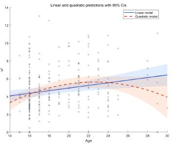
We thank the reviewer for this professional comment. In addition to the linear analyses, we further conducted exploratory analyses to examine potential non-linear relationships between age and the model parameters. Specifically, we fit LMMs for each of the four parameters as outcomes (α+, α-, β, and ω). The fixed effects included age, a quadratic age term, and gender, and the random effects included subject-specific random intercepts and random slopes for age and gender. Model comparison using BIC did not indicate improvement for the quadratic models over the linear models for α⁺ (ΔBIC_{quadratic-linear} = 5.09), α^-(ΔBIC_{quadratic-linear} = 3.04), β (ΔBIC_{quadratic-linear} = 3.9), or ω (ΔBIC_{quadratic-linear}= 0). Moreover, the quadratic age term was not significant for α⁺, α⁻, or β (all ps > 0.10). For ω, we observed a significant linear age effect (b = 1.41, t = 2.65, p = 0.009) and a significant quadratic age effect (b = −0.03, t = −2.39, p = 0.018; see Author response image 1). This pattern is broadly consistent with the group effect reported in the main text. The shaded area in the figure represents the 95% confidence interval. As shown, the interval widens at older ages (≥ 26 years) due to fewer participants in that range, which limits the robustness of the inferred quadratic effect. In consideration of the limited precision at older ages and the lack of BIC improvement, we did not emphasize the quadratic effect in the revised manuscript and present these results here as exploratory.

Author response image 1.

Linear and quadratic model fits showing the relationship between age and the ω parameter, with 95% confidence intervals.

(Q4) Finally, the two age groups compared - adolescents (high school students) and adults (university students) - differ not only in age but also in sociocultural and economic backgrounds. High school students are likely more homogenous in regional background (e.g., Beijing locals), while university students may be drawn from a broader geographic and socioeconomic pool. Additionally, differences in financial independence, family structure (e.g., single-child status), and social network complexity may systematically affect cooperative behavior and valuation of rewards. Although these factors are difficult to control fully, the authors should more explicitly address the extent to which their findings reflect biological development versus social and contextual influences.

We appreciate this comment. Indeed, adolescents (high school students) and adults (university students) differ not only in age but also in sociocultural and socioeconomic backgrounds. In our study, all participants were recruited from Beijing and surrounding regions, which helps minimize large regional and cultural variability. Moreover, we accounted for individual-level random effects and included participants’ social value orientation (SVO) as an individual difference measure.

Nonetheless, we acknowledge that other contextual factors, such as differences in financial independence, socioeconomic status, and social experience—may also contribute to group differences in cooperative behavior and reward valuation. Although our results are broadly consistent with developmental theories of reward sensitivity and social decisionmaking, sociocultural influences cannot be entirely ruled out. Future work with more demographically matched samples or with socioeconomic and regional variables explicitly controlled will help clarify the relative contributions of biological and contextual factors. Accordingly, we have revised the Discussion to include the following statement:

“Third, although both age groups were recruited from Beijing and nearby regions, minimizing major regional and cultural variation, adolescents and adults may still differ in socioeconomic status, financial independence, and social experience. Such contextual differences could interact with developmental processes in shaping cooperative behavior and reward valuation. Future research with demographically matched samples or explicit measures of socioeconomic background will help disentangle biological from sociocultural influences.”

Reviewer #3 (Public review):

Summary:

Wu and colleagues find that in a repeated Prisoner's Dilemma, adolescents, compared to adults, are less likely to increase their cooperation behavior in response to repeated cooperation from a simulated partner. In contrast, after repeated defection by the partner, both age groups show comparable behavior.

To uncover the mechanisms underlying these patterns, the authors compare eight different models. They report that a social reward learning model, which includes separate learning rates for positive and negative prediction errors, best fits the behavior of both groups. Key parameters in this winning model vary with age: notably, the intrinsic value of cooperating is lower in adolescents. Adults and adolescents also differ in learning rates for positive and negative prediction errors, as well as in the inverse temperature parameter.

Strengths:

The modeling results are compelling in their ability to distinguish between learned expectations and the intrinsic value of cooperation. The authors skillfully compare relevant models to demonstrate which mechanisms drive cooperation behavior in the two age groups.

We thank the reviewer’s recognition of our work’s strengths.

Weaknesses:

(Q1) Some of the claims made are not fully supported by the data:

The central parameter reflecting preference for cooperation is positive in both groups. Thus, framing the results as self-interest versus other-interest may be misleading.

We thank the reviewer for this insightful comment. In the social reward model, the cooperation preference parameter is positive by definition, as defection in the repeated rPDG always yields a +2 monetary advantage regardless of the partner’s action. This positive value represents the additional subjective reward assigned to mutual cooperation (e.g., reciprocity value) that counterbalances the monetary gain from defection. Although the estimated social reward parameter ω was positive, the effective advantage of cooperation is Δ=p×ω−2. Given participants’ inferred beliefs p, Δ was negative for most trials (p×ω<2), indicating that the social reward was insufficient to offset the +2 advantage of defection. Thus, both adolescents and adults valued cooperation positively, but adolescents’ smaller ω and weaker responsiveness to sustained partner cooperation suggest a stronger weighting on immediate monetary payoffs.

In this light, our framing of adolescents as more self-interested derives from their behavioral pattern: even when they recognized sustained partner cooperation and held high expectations of partner cooperation, adolescents showed lower cooperative behavior and reciprocity rewards compared with adults. Whereas adults increased cooperation after two or three consecutive partner cooperations, this pattern was absent among adolescents. We therefore interpret their behavior as relatively more self-interested, reflecting reduced sensitivity to the social reward from mutual cooperation rather than a categorical shift from self-interest to other-interest, as elaborated in the Discussion.

(Q2) It is unclear why the authors assume adolescents and adults have the same expectations about the partner's cooperation, yet simultaneously demonstrate age-related differences in learning about the partner. To support their claim mechanistically, simulations showing that differences in cooperation preference (i.e., the w parameter), rather than differences in learning, drive behavioral differences would be helpful.

We thank the reviewer for raising this important point. In our model, both adolescents and adults updated their beliefs about partner cooperation using an asymmetric reinforcement learning (RL) rule. Although adolescents exhibited a higher positive and a lower negative learning rate than adults, the two groups did not differ significantly in their overall updating of partner cooperation probability (Fig. 4a-b). We then examined the social reward parameter ω, which was significantly smaller in adolescents and determined the intrinsic value of mutual cooperation (i.e., p×ω). This variable differed significantly between groups and closely matched the behavioral pattern.

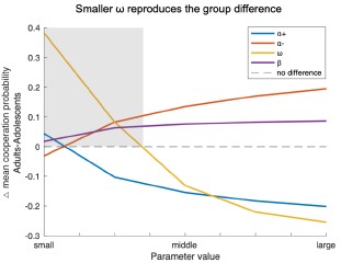
Following the reviewer’s suggestion, we conducted additional simulations varying one model parameter at a time while holding the others constant. The difference in mean cooperation probability between adults and adolescents served as the index (positive = higher cooperation in adults). As shown in the Author response image 2, decreases in ω most effectively reproduced the observed group difference (shaded area), indicating that age-related differences in cooperation are primarily driven by variation in the social reward parameter ω rather than by others.

Author response image 2.

Simulation results showing how variations in each model parameter affect the group difference in mean cooperation probability (Adults – Adolescents). Based on the bestfitting Model 8 and parameters estimated from all participants, each line represents one parameter (i.e., α+, α-, ω, β) systematically varied within the tested range (α±:0.1–0.9; ω, β:1–9) while other parameters were held constant. Positive values indicate higher cooperation in adults. Smaller ω values most strongly reproduced the observed group difference, suggesting that reduced social reward weighting primarily drives adolescents’ lower cooperation.

(Q3) Two different schedules of 120 trials were used: one with stable partner behavior and one with behavior changing after 20 trials. While results for order effects are reported, the results for the stable vs. changing phases within each schedule are not. Since learning is influenced by reward structure, it is important to test whether key findings hold across both phases.

We thank the reviewer for this thoughtful and professional comment. In our GLMM and LMM analyses, we focused on trial order rather than explicitly including the stable vs. changing phase factor, due to concerns about multicollinearity. In our design, phases occur in specific temporal segments, which introduces strong collinearity with trial order. In multi-round interactions, order effects also capture variance related to phase transitions.

Nonetheless, to directly address this concern, we conducted additional robustness analyses by adding a phase variable (stable vs. changing) to GLMM1, LMM1, and LMM3 alongside the original covariates. Across these specifications, the key findings were replicated (see GLMM_sup2 and LMM_sup4–5; Tables 9-11), and the direction and significance of main effects remained unchanged, indicating that our conclusions are robust to phase differences.

(Q4) The division of participants at the legal threshold of 18 years should be more explicitly justified. The age distribution appears continuous rather than clearly split. Providing rationale and including continuous analyses would clarify how groupings were determined.

We thank the reviewer for this thoughtful comment. We divided participants at the legal threshold of 18 years for both conceptual and practical reasons grounded in prior literature and policy. In many countries and regions, 18 marks the age of legal majority and is widely used as the boundary between adolescence and adulthood in behavioral and clinical research. Empirically, prior studies indicate that psychosocial maturity and executive functions approach adult levels around this age, with key cognitive capacities stabilizing in late adolescence (Icenogle et al., 2019; Tervo-Clemmens et al., 2023). We have clarified this rationale in the Introduction section of the revised manuscript.

“Based on legal criteria for majority and prior empirical work, we adopt 18 years as the boundary between adolescence and adulthood (Icenogle et al., 2019; Tervo-Clemmens et al., 2023).”

We fully agree that the underlying age distribution is continuous rather than sharply divided. To address this, we conducted additional analyses treating age as a continuous predictor (see GLMM_sup1 and LMM_sup1–3; Tables S1-S4), which generally replicated the patterns observed with the categorical grouping. Nevertheless, given the limited age range of our sample, the generalizability of these findings to fine-grained developmental differences remains constrained. Therefore, our primary analyses continue to focus on the contrast between adolescents and adults, rather than attempting to model a full developmental trajectory.

(Q5) Claims of null effects (e.g., in the abstract: "adults increased their intrinsic reward for reciprocating... a pattern absent in adolescents") should be supported with appropriate statistics, such as Bayesian regression.

We thank the reviewer for highlighting the importance of rigor when interpreting potential null effects. To address this concern, we conducted Bayes factor analyses of the intrinsic reward for reciprocity and reported the corresponding BF10 for all relevant post hoc comparisons. This approach quantifies the relative evidence for the alternative versus the null hypothesis, thereby providing a more direct assessment of null effects. The analysis procedure is now described in the Methods and Materials section:

“Post hoc comparisons were conducted using Bayes factor analyses with MATLAB’s bayesFactor Toolbox (version v3.0, Krekelberg, 2024), with a Cauchy prior scale σ = 0.707.”

(Q6) Once claims are more closely aligned with the data, the study will offer a valuable contribution to the field, given its use of relevant models and a well-established paradigm.

We are grateful for the reviewer’s generous appraisal and insightful comments.

Recommendations for the authors:

Reviewer #1 (Recommendations for the authors):

(1) I commend the authors on a well-structured, clear, and interesting piece of work. I have several questions and recommendations that, if addressed, I believe will strengthen the manuscript.

We thank the reviewer for commending the organization of our paper.

(2) Introduction: - Why use a zero-sum (Prisoner's Dilemma; PD) versus a mixed-motive game (e.g. Trust Task) to study cooperation? In a finite set of rounds, the dominant strategy can be to defect in a PD.

We thank the reviewer for this helpful comment. We agree that both the rationale for using the repeated Prisoner’s Dilemma (rPDG) and the limitations of this framework should be clarified. We chose the rPDG to isolate the core motivational conflict between selfinterest and joint welfare, as its symmetric and simultaneous structure avoids the sequential trust and reputation dependencies/accumulation inherent to asymmetric tasks such as the Trust Game (King-Casas et al., 2005; Rilling et al., 2002).

Although a finitely repeated rPDG theoretically favors defection, extensive prior research shows that cooperation can still emerge in long repeated interactions when players rely on learning and reciprocity rather than backward induction (Rilling et al., 2002; Fareri et al., 2015). Our design employed 120 consecutive rounds, allowing participants to update expectations about partner behavior and to establish stable reciprocity patterns over time. We have added the following clarification to the Introduction:

“The rPDG provides a symmetric and simultaneous framework that isolates the motivational conflict between self-interest and joint welfare, avoiding the sequential trust and reputation dynamics characteristic of asymmetric tasks such as the Trust Game (Rilling et al., 2002; King-Casas et al., 2005)”

(3) Methods:

Did the participants know how long the PD would go on for?

Were the participants informed that the partner was real/simulated?

Were the participants informed that the partner was going to be the same for all rounds?

We thank the reviewer for the meticulous review work, which helped us present the experimental design and reporting details more clearly. the following clarifications: I. Participants were not informed of the total number of rounds in the rPDG. This prevented endgame expectations and avoided distraction from counting rounds, which could introduce additional effects. II. Participants were told that their partner was another human participant in the laboratory. However, the partner’s behavior was predetermined by a computer program. This design enabled tighter experimental control and ensured consistent conditions across age groups, supporting valid comparisons. III. Participants were informed that they would interact with the same partner across all rounds, aligning with the essence of a multiround interaction paradigm and stabilizing partner-related expectations. For transparency, we have clarified these points in the Methods and Materials section:

“Participants were told that their partner was another human participant in the laboratory and that they would interact with the same partner across all rounds. However, in reality, the actions of the partner were predetermined by a computer program. This setup allowed for a clear comparison of the behavioral responses between adolescents and adults. Participants were not informed of the total number of rounds in the rPDG.”

(4) The authors mention that an SVO was also recorded to indicate participant prosociality. Where are the results of this? Did this track game play at all? Could cooperativeness be explained broadly as an SVO preference that penetrated into game-play behaviour?

We thank the reviewer for pointing this out. We agree that individual differences in prosociality may shape cooperative behavior, so we conducted additional analyses incorporating SVO. Specifically, we extended GLMM1 and LMM3 by adding the measured SVO as a fixed effect with random slopes, yielding GLMM_sup3 and LMM_sup6 (Tables 12–13). The results showed that higher SVO was associated with greater cooperation, whereas its effect on the reward for reciprocity was not significant. Importantly, the primary findings remained unchanged after controlling for SVO. These results indicate that cooperativeness in our task cannot be explained solely by a broad SVO preference, although a more prosocial orientation was associated with greater cooperation. We have reported these analyses and results in the Appendix Analysis section.

(5) Why was AIC chosen rather an BIC to compare model dominance?

Sorry for the lack of clarification. Both the Akaike Information Criterion (AIC, Akaike, 1974) and Bayesian Information Criterion (BIC, Schwarz, 1978) are informationtheoretic criterions for model comparison, neither of which depends on whether the models to be compared are nested to each other or not (Burnham et al., 2002). We have added the following clarification into the Methods.

“We chose to use the AICc as the metric of goodness-of-fit for model comparison for the following statistical reasons. First, BIC is derived based on the assumption that the “true model” must be one of the models in the limited model set one compares (Burnham et al., 2002; Gelman & Shalizi, 2013), which is unrealistic in our case. In contrast, AIC does not rely on this unrealistic “true model” assumption and instead selects out the model that has the highest predictive power in the model set (Gelman et al., 2014). Second, AIC is also more robust than BIC for finite sample size (Vrieze, 2012).”

(6) I believe the model fitting procedure might benefit from hierarchical estimation, rather than maximum likelihood methods. Adolescents in particular seem to show multiple outliers in a^+ and w^+ at the lower end of the distributions in Figure S2. There are several packages to allow hierarchical estimation and model comparison in MATLAB (which I believe is the language used for this analysis;

see https://journals.plos.org/ploscompbiol/article?id=10.1371/journal.pcbi.1007043).

We thank the reviewer for this helpful comment and for referring us to relevant methodological work (Piray et al., 2019). We have addressed this point by incorporating hierarchical Bayesian estimation, which effectively mitigates outlier effects and improves model identifiability. The results replicated those obtained with MLE fitting and further revealed group-level differences in key parameters. Please see our detailed response to Reviewer#1 Q1 for the full description of this analysis and results.

(7) Results: Model confusion seems to show that the inequality aversion and social reward models were consistently confused with the baseline model. Is this explained or investigated? I could not find an explanation for this.

The apparent overlap between the inequality aversion (Model 4) and social reward (Model 5) models in the recovery analysis likely arises because neither model includes a learning mechanism, making them unable to capture trial-by-trial adjustments in this dynamic task. Consequently, both were best fit by the baseline model. Please see Response to Reviewer #1 Q3 for related discussion.

(8) Figures 3e and 3f show the correlation between asymmetric learning rates and age. It seems that both a^+ and a^- are around 0.35-0.40 for young adolescents, and this becomes more polarised with age. Could it be that with age comes an increasing discernment of positive and negative outcomes on beliefs, and younger ages compress both positive and negative values together? Given the higher stochasticity in younger ages (\beta), it may also be that these values simply represent higher uncertainty over how to act in any given situation within a social context (assuming the differences in groups are true).

We appreciate this insightful interpretation. Indeed, both α+ and α- cluster around 0.35–0.40 in younger adolescents and become increasingly polarized with age, suggesting that sensitivity to positive versus negative feedback is less differentiated early in development and becomes more distinct over time. This interpretation remains tentative and warrants further validation. Based on this comment, we have revised the Discussion to include this developmental interpretation.

We also clarify that in our model β denotes the inverse temperature parameter; higher β reflects greater choice precision and value sensitivity, not higher stochasticity. Accordingly, adolescents showed higher β values, indicating more value-based and less exploratory choices, whereas adults displayed relatively greater exploratory cooperation. These group differences were also replicated using hierarchical Bayesian estimation (see Response to Reviewer #1 Q1). In response to this comment, we have added a statement in the Discussion highlighting this developmental interpretation.

“Together, these findings suggest that the differentiation between positive and negative learning rates changes with age, reflecting more selective feedback sensitivity in development, while higher β values in adolescents indicate greater value sensitivity. This interpretation remains tentative and requires further validation in future research.”

(9) A parameter partial correlation matrix (off-diagonal) would be helpful to understand the relationship between parameters in both adolescents and adults separately. This may provide a good overview of how the model properties may change with age (e.g. a^+'s relation to \beta).

We thank the reviewer for this helpful comment. We fully agree that a parameter partial correlation matrix can further elucidate the relationships among parameters. Accordingly, we conducted a partial correlation analysis and added the visually presented results to the revised manuscript as Figure 2-figure supplement 4.

(10) It would be helpful to have Bayes Factors reported with each statistical tests given that several p-values fall within the 0.01 and 0.10.

We thank the reviewer for this important recommendation. We have conducted Bayes factor analyses and reported BF10 for all relevant post hoc comparisons. We also clarified our analysis in the Methods and Materials section:

“Post hoc comparisons were conducted using Bayes factor analyses with MATLAB’s bayesFactor Toolbox (version v3.0, Krekelberg, 2024), with a Cauchy prior scale σ = 0.707.”

(11) Discussion: I believe the language around ruling out failures in mentalising needs to be toned down. RL models do not enable formal representational differences required to assess mentalising, but they can distinguish biases in value learning, which in itself is interesting. If the authors were to show that more complex 'ToM-like' Bayesian models were beaten by RL models across the board, and this did not differ across adults and adolescents, there would be a stronger case to make this claim. I think the authors either need to include Bayesian models in their comparison, or tone down their language on this point, and/or suggest ways in which this point might be more thoroughly investigated (e.g., using structured models on the same task and running comparisons: https://journals.plos.org/plosone/article?id=10.1371/journal.pone.0087619).

We thank the reviewer for the comments. Please see our response to Reviewer 1 (Appraisal & Discussion section) for details.

Reviewer #2 (Recommendations for the authors):

(1) The authors may want to show the winning model earlier (perhaps near the beginning of the Results section, when model parameters are first mentioned).

We thank the reviewer for this suggestion. We agree that highlighting the winning model early improves clarity. Currently, we have mentioned the winning model before the beginning of the Results section. Specifically, in the penultimate paragraph of the Introduction we state:

“We identified the asymmetric RL learning model as the winning model that best explained the cooperative decisions of both adolescents and adults.”

Reviewer #3 (Recommendations for the authors):

(1) In addition to the points mentioned above, I suggest the following:

Clarify plots by clearly explaining each variable. In particular, the indices 1 vs. 1,2 vs 1,2,3 were not immediately understandable.

We thank the reviewer for this suggestion. We agree that the indices were not immediately clear. We have revised the figure captions (Figure 1 and 4) to explicitly define these terms more clearly:

“The x-axis represents the consistency of the partner’s actions in previous trials (t₋₁: last trial; t_−1,2: last two trials;_t−1,2,3: last three trials).”

(2) It's unclear why the index stops at 3. If this isn't the maximum possible number of consecutive cooperation trials, please consider including all relevant data, as adolescents might show a trend similar to adults over more trials.

We thank the reviewer for raising this point. In our exploratory analyses, we also examined longer streaks of consecutive partner cooperation or defection (up to four or five trials). Two empirical considerations led us to set the cutoff at three in the final analyses. First, the influence of partner behavior diminished sharply with temporal distance. In both GLMMs and LMMs, coefficients for earlier partner choices were small and unstable, and their inclusion substantially increased model complexity and multicollinearity. This recency pattern is consistent with learning and decision models emphasizing stronger weighting of recent evidence (Fudenberg & Levine, 2014; Fudenberg & Peysakhovich, 2016). Second, streaks longer than three were rare, especially among some participants, leading to data sparsity and inflated uncertainty. Including these sparse conditions risked biasing group estimates rather than clarifying them. Balancing informativeness and stability, we therefore restricted the index to three consecutive partner choices in the main analyses, which we believe sufficiently capture individuals’ general tendencies in reciprocal cooperation.

(3) The term "reciprocity" may not be necessary. Since it appears to reflect a general preference for cooperation, it may be clearer to refer to the specific behavior or parameter being measured. This would also avoid confusion, especially since adolescents do show negative reciprocity in response to repeated defection.

We thank you for this comment. In our work, we compute the intrinsic reward for reciprocity as p × ω, where p is the partner cooperation expectation and ω is the cooperation preference. In the rPDG, this value framework manifests as a reciprocity-derived reward: sustained mutual cooperation maximizes joint benefits, and the resulting choice pattern reflects a value for reciprocity, contingent on the expected cooperation of the partner. This quantity enters the trade-off between U_cooperation and U_defection and captures the participant’s intrinsic reward for reciprocity versus the additional monetary reward payoff of defection. Therefore, we consider the term “reciprocity” an acceptable statement for this construct.

(4) Interpretation of parameters should closely reflect what they specifically measure.

We thank the reviewer for pointing this out. We have refined the relevant interpretations of parameters in the current Results and Discussion sections.

(5) Prior research has shown links between Theory of Mind (ToM) and cooperation (e.g., Martínez-Velázquez et al., 2024). It would be valuable to test whether this also holds in your dataset.

We thank the reviewer for this thoughtful comment. Although we did not directly measure participants’ ToM, our design allowed us to estimate participants’ trial-by-trial inferences (i.e., expectations) about their partner’s cooperation probability. We therefore treat these cooperation expectations as an indirect representation for belief inference, which is related to ToM processes. To test whether this belief-inference component relates to cooperation in our dataset, we further conducted an exploratory analysis (GLMM_sup4) in which participants’ choices were regressed on their cooperation expectations, group, and the group × cooperation-expectation interaction, controlling for trial number and gender, with random effects. Consistent with the ToM–cooperation link in prior research (MartínezVelázquez et al., 2024), participants’ expectations about their partner’s cooperation significantly predicted their cooperative behavior (Table 14), suggesting that decisions were shaped by social learning about others’ inferred actions. Moreover, the interaction between group and cooperation expectation was not significant, indicating that this inference-driven social learning process likely operates similarly in adolescents and adults. This aligns with our primary modeling results showing that both age groups update beliefs via an asymmetric learning process. We have reported these analyses in the Appendix Analysis section.

(6) More informative table captions would help the reader. Please clarify how variables are coded (e.g., is female = 0 or 1? Is adolescent = 0 or 1?), to avoid the need to search across the manuscript for this information.

We thank the reviewer for raising this point. We have added clear and standardized variable coding in the table notes of all tables to make them more informative and avoid the need to search the paper. We have ensured consistent wording and formatting across all tables.

(7) I hope these comments are helpful and support the authors in further strengthening their manuscript.

We thank the three reviewers for their comments, which have been helpful in strengthening this work.

References

(1) Fudenberg, D., & Levine, D. K. (2014). Recency, consistent learning, and Nash equilibrium. Proceedings of the National Academy of Sciences of the United States of America, 111(Suppl. 3), 10826–10829. https://doi.org/10.1073/pnas.1400987111.

(2) Fudenberg, D., & Peysakhovich, A. (2016). Recency, records, and recaps: Learning and nonequilibrium behavior in a simple decision problem. ACM Transactions on Economics and Computation, 4(4), Article 23, 1–18. https://doi.org/10.1145/2956581

(3) Hackel, L., Doll, B., & Amodio, D. (2015). Instrumental learning of traits versus rewards: Dissociable neural correlates and effects on choice. Nature Neuroscience, 18, 1233– 1235. https://doi.org/10.1038/nn.4080

(4) Icenogle, G., Steinberg, L., Duell, N., Chein, J., Chang, L., Chaudhary, N., Di Giunta, L., Dodge, K. A., Fanti, K. A., Lansford, J. E., Oburu, P., Pastorelli, C., Skinner, A. T.Sorbring, E., Tapanya, S., Uribe Tirado, L. M., Alampay, L. P., Al-Hassan, S. M.,Takash, H. M. S., & Bacchini, D. (2019). Adolescents’ cognitive capacity reaches adult levels prior to their psychosocial maturity: Evidence for a “maturity gap” in a multinational, cross-sectional sample. Law and Human Behavior, 43(1), 69–85. https://doi.org/10.1037/lhb0000315

(5) Krekelberg, B. (2024). Matlab Toolbox for Bayes Factor Analysis (v3.0) [Computer software]. Zenodo. https://doi.org/10.5281/zenodo.13744717

(6) Martínez-Velázquez, E. S., Ponce-Juárez, S. P., Díaz Furlong, A., & Sequeira, H. (2024). Cooperative behavior in adolescents: A contribution of empathy and emotional regulation? Frontiers in Psychology, 15,1342458. https://doi.org/10.3389/fpsyg.2024.1342458

(7) Tervo-Clemmens, B., Calabro, F. J., Parr, A. C., et al. (2023). A canonical trajectory of executive function maturation from adolescence to adulthood. Nature Communications, 14, 6922. https://doi.org/10.1038/s41467-023-42540-8

(8) King-Casas, B., Tomlin, D., Anen, C., Camerer, C. F., Quartz, S. R., & Montague, P. R. (2005). Getting to know you: reputation and trust in a two-person economic exchange. Science, 308(5718), 78-83. https://doi.org/10.1126/science.1108062

(9) Rilling, J. K., Gutman, D. A., Zeh, T. R., Pagnoni, G., Berns, G. S., & Kilts, C. D. (2002).A neural basis for social cooperation. Neuron, 35(2), 395-405. https://doi.org/10.1016/s0896-6273(02)00755-9

(10) Fareri, D. S., Chang, L. J., & Delgado, M. R. (2015). Computational substrates of social value in interpersonal collaboration. Journal of Neuroscience, 35(21), 8170-8180. https://doi.org/10.1523/JNEUROSCI.4775-14.2015

(11) Akaike, H. (2003). A new look at the statistical model identification. IEEE transactions on automatic control, 19(6), 716-723. https://doi.org/10.1109/TAC.1974.1100705

(12) Schwarz, G. (1978). Estimating the dimension of a model. The annals of statistics, 461464. https://doi.org/10.1214/aos/1176344136

(13) Burnham, K. P., & Anderson, D. R. (2002). Model selection and multimodel inference: A practical information-theoretic approach (2nd ed.). Springer.https://doi.org/10.1007/b97636

(14) Gelman, A., & Shalizi, C. R. (2013). Philosophy and the practice of Bayesian statistics. British Journal of Mathematical and Statistical Psychology, 66(1), 8–38. https://doi.org/10.1111/j.2044-8317.2011.02037.x

(15) Gelman, A., Carlin, J. B., Stern, H. S., Dunson, D. B., Vehtari, A., & Rubin, D. B. (2014). Bayesian data analysis (3rd ed.). Chapman and Hall/CRC. https://doi.org/10.1201/b16018

(16) Vrieze, S. I. (2012). Model selection and psychological theory: A discussion of the differences between the Akaike Information Criterion (AIC) and the Bayesian Information Criterion (BIC). Psychological Methods, 17(2), 228–243. https://doi.org/10.1037/a0027127

Video games can be both negative and positive. Negative because the screen time can cause behavioral issues. Positive because it could aid in the student's skillset to complete academic tasks.

While the data is not mainly negative, it is advised that screen time should be reduced to avoid a decrease in academic performance.

They're also told, "answer truthfully for a best case outcome"

Before the 1830s, newspapers were expensive and mostly for rich political nerds. Benjamin Day changed the game by making the paper smaller, using a faster press, and selling it for just a penny.

The Penny Press turned newspapers into the first true form of mass media.

The text states that Day slashed the price of the paper to a penny and utilized a two cylinder steam engine to massively increase production.

Because the paper became affordable and shifted its focus to human-interest stories rather than just dry politics, it reached the average person for the first time. This expanded the audience from a small elite group to the general public, creating the massmarket journalism we recognize today.

I have experienced this when modifying game files on my PC, finding the directory, opening a file, then finding even more files, and even more when opening one of those.

I think this still occurs in settings like video games. For example, tricking a new player into doing something that every experienced player knows doesn't work or negatively impacts the new player in some way. I see this most often when streamers are trying out a new game (typically well-known and the streamer is just late to playing it, like minecraft), where they suggest things they know are trolls. Something that comes to mind would be like playing a bed in the nether for Minecraft.

Misogyny on the internet seems to be more severe than in real life—especially in the realm of online gaming. At first, I thought this was because gaming is a space that glorifies skill and power, where authority is tied almost exclusively to “game performance,” and stereotypes about women being worse at games lead to a loss of discursive power. However, if misogyny was already pervasive in the early internet, then I think there must be other contributing factors and explanations as well.

Sartre pointed out the strategic advantage of the "bad faith" argument: one party treats the dialogue not as a search for truth, but as a game; the other party, however, is bound by norms (reason, evidence, politeness). Applied to modern trolling, this explains why "seriously responding" often fails—the opponent's goal is not to be persuaded, but to make you invest time and effort, lose patience, and appear "too serious" in the public sphere. Therefore, the strategy is often not to argue more forcefully, but to identify their incentive structure (wasting your time, disrupting order) and reduce your susceptibility to being exploited.

I noticed this in "depression quest" that there was no way of getting a sense of where you were in the game. For me, it made me connect better with my own personal journey through the story.

I found it interesting how broad this definition is and how well it fits many of the video games people play. As someone who plays a lot of games, I can think about how it applies to almost all of them that I am personally familiar with.

As a player, you feel the strong sense of power described in agency previously through solving puzzles and thinking outside of the box. You start to feel that you have outsmarted the game or the circumstances. This accomplished feeling leads to greater engagement with the narrative and gameplay elements.

Through the medium of a game, agency is limited but the environment is engineered in a way that makes helplessness as just another step or another obstacle adding to the enjoyment. Much like Odysseus, you're placed in a situation where there's not much to work with but through your agency you can make what there is of the situation to get out of it.

Great questions to be asking

This is totally understandable. No one would like to be deceived, the feeling of it I can tell that is not good. However this small sections makes me think that how awful it is, as I never realised that authenticity can be this serious. as it made us suspect on ourself that if we can make correct judgement of the posts in the social media. Once I saw a post that it said slide left to see the cat, it turns out to be an advertisement of a boring poorly made game, everyone in the comment was upset and angry.

I do feel like sharing ideas is not bad, when we need help, we don't always walk to the instructor maybe we just ask a classmate and have ideas and become to one another.

It's better to be safe than sorry! You don't want to guess yourself into a grade or a higher education. It's okay to ask questions to your peers or even your instructor.

Farewell words of Ophelia, in her madness, to the ladies of the court of the King of Denmark

"Thanks" in Cockney.

Pharmacist.

Abortion pills.

The barman is telling everyone to get out.

Released from military service.

Folk song.

"The Tempest."

The sound of the nightingale.

Mentions of abuse.

In medieval art, the dolphin was associated with love.

The panels of a coffered ceiling.

The first ecounter of Enea and Didone in Virgil's "Aeneid".

Shakespeare's "Antony and Cleopatra".

God of love.

Satyrical play of Thomas Middleton "A game at chess".

Although bulletin board systems originated decades ago, many websites today still use this forum-style structure. For example, the Dungeons & Dragons (D&D) community relies heavily on well-known bulletin board forums where players share discussions, homebrew rules, and game resources. Similarly, the fighting game MUGEN, which comes from the arcade era, has dedicated forums where users upload character models, stages, and other custom assets. These modern bulletin board systems show how this format continues to support niche communities by organizing discussions and resources in a clear, thread-based way.

In video games one who guides you learning a new game is often called a sherpa. They carry you, but you also remind them of how the game can be fun and not always competitive.

For mechanics, they wouldn't have as much work if beginners didn't break stuff to begin with :)

Rock climbing something repeatedly can feel like doing the same math problem over and over again but still getting the wrong answer until someone else comes over and shows you a new way to get to the solution.

Much like in playing a competitive video game it is extremely helpful to know callout locations with your friends to know where enemies might be. Or to know which items are more valuable to pick up.

Cars it is useful to know if your car is an inline-4 cylinder, V6 etc. Knowing your cars brake system if it vacuum boosted or hydro-boosted will help diagnosing issues etc.

When rock climbing understanding callouts of specific holds, how to belay, types of movements can really help you understand more when climbing with someone else.

Trying to compare this to another community I belong to would be having the tutorial mode on when playing a new game.

Working on an older car where the system is easier and there are a lot of YouTube videos out already on this.

In a rock climbing gym there are routes with grades on them to help people know which routes are going to be more approachable.

In the second verse, the rapper expands on the concept of developing wealth and obtaining financial freedom, which he defines as his only hope.

He also makes reference to his streaming platform, Tidal, which offers a million dollars worth of game through its music catalog for $9.99 a month. Tidal is just one of the many business ventures of the rapper.

In the closing lines, he mocks rappers who take "advances" - a form of loan that record labels offer to artists to finance their albums - and also the trend followed by some rappers on Instagram of showing off money by holding it close to their ears. He reveals, with a clever play on words, that there's a disconnect, we don't call that money over here.

In this song, Jay-Z is constantly pointing out at the importance of property and wealth. He is, therefore, to be considered a Black capitalist. He shows how he strongly believes in economic success as the principal means reaching some form of equality or, at least, some form of upliftment.

However, he does not really believe that wealth and status can be a proper shield from racism; thus, wealth is only a way to obtain a very partial equality.

The first verse is written from the perspective of Lamar's mom, dealing with a 7 year old Kendrick. The biggest fear of the kid is being whooped by his mother, that is constantly threatening him in order to teach the boy discipline.

The scenario Kendrick is depicting is also meant to represent the life of many poor African-Americans as the line County's building on my ass, tryna take my food stamps away is underlying. The Food Stamp Program is a program that provides food to low-income families.

Also, the line I beat yo' ass if you tell them social workers he live here is a reference to the “man in the house” rule, where welfare benefits would be denied to a family if a man resided in the house. Kendrick's mom is alluding to this rule.

The closing line gives the idea of how Kendrick's mom is determined to be the first reason of fear for the boy, and although it is for the reason for his own protection, this same sensation of fear will never leave him and will take more complex forms.

Quote: "Elevate your delivery game with GFS’ proven, tech-powered, multi-carrier logistics and operational excellence." Comment: Internal links - very important for this page in particular

• https://gfsdeliver.com/gfs-in-the-press/in-the-press-how-does-last-mile-delivery-affect-your-ecommerce-brand/
• https://gfsdeliver.com/blog/bringing-it-home-expert-tips-for-last-mile-delivery-in-the-homeware-industry/
• https://gfsdeliver.com/blog/final-mile-delivery-tracking-in-multi-carrier-shipping-to-handle-high-order-volumes/

eLife Assessment

This important study combines a two-person joint hand-reaching paradigm with game-theoretical modeling to examine whether, and how, one's reflexive visuomotor responses are modulated by a partner's control policy and cost structure. The study provides a solid and novel set of behavioral findings suggesting that involuntary visuomotor feedback is indeed modulated in the context of interpersonal coordination. The work will be of interest to cognitive scientists studying the motoric and social aspects of action control.

Reviewer #2 (Public review):

Summary:

Sullivan and colleagues studied the fast, involuntary, sensorimotor feedback control in interpersonal coordination. Using a cleverly designed joint-reaching experiment that separately manipulated the accuracy demands for a pair of participants, they demonstrated that the rapid visuomotor feedback response of a human participant to a sudden visual perturbation is modulated by his/her partner's control policy and cost. The behavioral results are well-matched with the predictions of the optimal feedback control framework implemented with the dynamic game theory model. Overall, the study provides an important and novel set of results on the fast, involuntary feedback response in human motor control, in the context of interpersonal coordination.

Review:

Sullivan and colleagues investigated whether fast, involuntary sensorimotor feedback control is modulated by the partner's state (e.g., cost and control policy) during interpersonal coordination. They asked a pair of participants to make a reaching movement to control a cursor and hit a target, where the cursor's position was a combination of each participant's hand position. To examine fast visuomotor feedback response, the authors applied a sudden shift in either the cursor (experiment 1) or the target (experiment 2) position in the middle of movement. To test the involvement of partner's information in the feedback response, they independently manipulated the accuracy demand for each participant by varying the lateral length of the target (i.e., a wider/narrower target has a lower/higher demand for correction when movement is perturbed). Because participants could also see their partner's target, they could theoretically take this information (e.g., whether their partner would correct, whether their correction would help their partner, etc.) into account when responding to the sudden visual shift. Computationally, the task structure can be handled using dynamic game theory, and the partner's feedback control policy and cost function are integrated into the optimal feedback control framework. As predicted by the model, the authors demonstrated that the rapid visuomotor feedback response to a sudden visual perturbation is modulated by the partner's control policy and cost. When their partner's target was narrow, they made rapid feedback corrections even when their own target was wide (no need for correction), suggesting integration of their partner's cost function. Similarly, they made corrections to a lesser degree when both targets were narrower than when the partner's target was wider, suggesting that the feedback correction takes the partner's correction (i.e., feedback control policy) into account.

The strength of the current paper lies in the combination of clever behavioral experiments that independently manipulate each participant's accuracy demand and a sophisticated computational approach that integrates optimal feedback control and dynamic game theory. Both the experimental design and data analysis sound good. While the main claim is well-supported by the results, the only current weakness is the lack of discussion of limitations and an alternative explanation. Adding these points will further strengthen the paper.

I would like to clarify a point regarding the discovery of lymphatic-like vessels in the brain. The preprint appears to hint towards positioning it as the first report of this finding. However, the first published study on this subject was by Chang et al.(Ref 1 below). The authors reported on the presence and characteristics (diameters, origin, length, depth and regulation by stress) of deep brain lymphatic vessels. Their work was subsequently followed by two other independent studies (Ref 2 and 3). All studies were reviewed in a review article in 2024 (https://www.sciopen.com/article/10.26599/SAB.2024.9060001?issn=2709-1325).

Therefore, the preprint would represent a fourth report—not the first—of this discovery. It is concerning that previous foundational work has been either overlooked or cited in a misleading manner.

References 1. Chang J, Guo B, Gao Y, Li W, Tong X, Feng Y, et al. Characteristic Features of Deep Brain Lymphatic Vessels and Their Regulation by Chronic Stress. Research (Washington, DC), 2023, 6:0120.

1. Öz E. 'Game changer' method lets scientists peer into mice. Science (New York, NY), 2023, 380(6644):443.

2. Liu X-G, Hua Q, Peng T-T, Chang K-X, Deng C-G, Zhang J-N, et al. Histomorphological analysis of perfusion parameters and CNS lymphatic vessels in mice: an experimental method study. NeuroReport, 2024, 35(3).

Robust

This web using clean HTML and work well with different browsers (Chrome, Safari, Firefox,etc). The content processed correctly by tools as I tested the Safari screen reader.

Next chapter also tried to problematise the idea of serious or commerical games as the saviours of gaming, from the lens that they are embeded in a chokepoint technofeudalism that translates volunteering, modding, community building, hacking, and charitative donations, as a solutionist fix that doesn't change the system, rather tries to cover its holes. Against the idea to mobilise the youngster slackers with mainstream video games, it develops the Shirky principle idea that actually, this contributes to the concentration and surveillance data grab of BigTech that's part of the problem. It specially attacked a book cited in multiple chapters: Ellen Middaugh, and Chris Evans’ The civic potential of video games.

It argues from Baudrillard's complicit euphoria, cult of the ego, hedonism, the society of the spectacle, consumerism, the maximisation - compulsive collection of diverse pleasures. I deleted it because it doesn't provide alternative paths, like how against instrumental solutionism, games must die, and culture must die too, but it must be reborn again and again breaking the Overton window of what's accepted, reborn with non-conventional meanings and feelings, reborn without its elitist concentrated play, without its assumptions (with alternatives instead), and reborn with coordinating transgressive revolution ingrained on it.

Footnote 2 from this chapter expands on this a bit.

And yet, September 12th is too much simple. As a simulation, it only conveys the ideal of violence begets violence, but such a principle can leave players with a sour patronising mouth taste of "I already knew that". The world is more complex, but immersion and its mastery from habit also difficult periodically leaving it and challenging one's perspectives, like it happens in McDonald's, Frostpunk, Mini Metro, Democracy, or Cities Skylines. These simulations can be much more insightful, but the requirement is that players know how to read.

From the text: Frasca proposes that players, not only game designers, potentially impact the ultimate rhetorical “outcome” of a game by channeling the course of play into directions unimagined by the game-maker (2003b, 228). Frasca calls upon Brazilian theater director Augusto Boal’s “Theater of the Oppressed” as a model for how a game can depart from Aristotlean narrative closure. Frasca writes “one of [Boal’s] most popular techniques, re-enacts the same play several times by allowing diffferent audience members to get into the stage and take the protagonist’s role”.

This happens in hacking, modding, and maker cultures, cheating in GTA, in Card/Collection games to give yourself the console and obtain whichever item, like how Minecraft creative mode allows. This "becoming" the designer enables "seeing" through its lens. Counter play can also happen when steering against stereotypical gameful intentions, as with Disaster Sims in the series with the same name, or as prompted in reflection simulation games like Proteus.

That's where designing and maker precepts also come in. In reading a game, in watching it reflectively, in playing as a designer, a deconstructor. This is not often taught to players. An issue with the argument is that when they leave, they may leave out of frustration, which can cause missunderstandings and not prompt reflection. It can make these players abstain from simulation genres as a whole, and engage in more arcade "neutral" (immediate gratification) f2p titles.

Flash games died, no... Adobe killed them. Flash games were free. They lived on Kongregate, on Newgrounds, on Miniclip.

As someone learning a new language I have had this exact experience! I started playing a game in Japanese when I was younger without speaking any. I recently started playing again and not only can I understand so much more, I can read and use context to learn new stuff!! It's been such a cool experience!

Indigenous people here are being talked about like if they were pieces in a game of chess rather than actual people. It's a common theme I've seen throughout many of these passages.

As the eastern lands were taken up, migration flowed across them to the west. Daniel Boone, the great backwoodsman, who combined the occupations of hunter, trader, cattle-raiser, farmer, and surveyor -- learning, probably from the traders, of the fertility of the lands of the upper Yadkin, where the traders were wont to rest as they took their way to the Indians, left his Pennsylvania home with his father, and passed down the Great Valley road to that stream.

Learning from a trader whose posts were on the Red River in Kentucky of its game and rich pastures, he pioneered the way for the farmers to that region. Thence he passed to the frontier of Missouri, where his settlement was long a landmark on the frontier. Here again he helped to open the way for civilization, finding salt licks, and trails, and land.

Prob predictable

RPI game design major

Like 60s rhetoric education

Like early days of rhetcomp but with corporate funding pressure

Of course

Synthèse : Prévention et lutte contre le harcèlement scolaire (Webinaire FCPE-MAE)

Résumé exécutif

Le harcèlement scolaire est une problématique systémique qui touche environ un élève sur dix.

Face à ce constat, le webinaire organisé par la FCPE et la MAE souligne l'impératif d'une action concertée entre parents, professionnels de l'éducation et partenaires institutionnels.

L'approche défendue repose sur trois piliers : la détection précoce des signaux d'alerte, l'utilisation d'outils pédagogiques adaptés à chaque tranche d'âge (de la maternelle au lycée), et une coéducation active.

La MAE, partenaire historique de l'enseignement public, met à disposition des ressources gratuites et agréées par le Ministère de l'Éducation nationale, s'inscrivant notamment dans le cadre du programme national Phare.

L'objectif central est de briser le silence et de passer d'une logique de réaction à une culture de prévention durable.

--------------------------------------------------------------------------------

1. Analyse du phénomène de harcèlement scolaire

Définitions et mécanismes

Le harcèlement se caractérise par un rapport de force déséquilibré où une ou plusieurs personnes exercent une pression ou un contrôle répété sur une victime.

• Formes constatées : Insultes, moqueries, rumeurs, humiliations et mises à l'écart.

• Évolution : Les situations débutent souvent par des faits perçus comme « pour rire » avant de déraper vers une souffrance physique et psychologique grave.

Le défi du cyber-harcèlement

Le cyber-harcèlement transpose ces violences sur les réseaux sociaux, les messageries, les forums et les jeux vidéo.

• Gravité : La circulation des attaques est extrêmement rapide et peut toucher une audience très large.

• Traces : Les agressions en ligne laissent des marques durables et ne s'arrêtent pas aux portes de l'école.

• Statistique clé : Un collégien sur cinq a déjà été victime d'au moins un acte de cyber-violence répété.

Signaux d'alerte pour les adultes

La vigilance des parents et des enseignants doit se porter sur les changements de comportement :

• État émotionnel : Isolement, colère, tristesse subite.

• Vie scolaire : Baisse des résultats, refus d'aller en cours ou de participer à certaines activités.

• Santé physique : Troubles du sommeil, de l'appétit, maux de tête ou de ventre fréquents.

• Signes matériels : Vêtements abîmés, perte d'effets personnels.

• Rapport au numérique : Enfant qui cache son téléphone ou le consulte avec une angoisse permanente.

--------------------------------------------------------------------------------

2. Le cadre institutionnel et l'engagement de la MAE

Un acteur historique

Fondée en 1932 par des enseignants, la MAE est une mutuelle issue de l'économie sociale et solidaire. Elle bénéficie de l'agrément national du Ministère de l'Éducation nationale pour intervenir dans les établissements scolaires.

Soutien aux familles et garanties

Au-delà de la prévention, la MAE propose des protections spécifiques dans ses contrats d'assurance :

• Soutien psychologique en cas de harcèlement avéré.

• Assistance juridique en cas d'atteinte à l'image de l'enfant.

• Aide à la suppression de contenus malveillants sur Internet.

Le programme Phare

Les outils présentés s'inscrivent dans le dispositif ministériel Phare, qui repose sur cinq piliers :

1. Éduquer pour prévenir les phénomènes de harcèlement.

2. Former une communauté protectrice autour des élèves.

3. Intervenir efficacement sur les situations de harcèlement.

4. Associer les parents et les partenaires.

5. Mobiliser les instances de démocratie scolaire (CESCE).

--------------------------------------------------------------------------------

3. Ressources et outils pédagogiques par cycles

Les ressources proposées sont gratuites et conçues en collaboration avec des professionnels de l'éducation (notamment l'AGEEM pour le premier degré).

Pour les 3 - 11 ans (Maternelle et Élémentaire)

| Outil | Description | Objectif | | --- | --- | --- | | Album "Maël le roi des bêtises" | Support de 25 pages avec cahier d'activités. | Apprendre le respect des différences et le vivre-ensemble dès le plus jeune âge. | | BD "Main dans la main" | Format innovant (illustration à gauche, exploitation pédagogique à droite). | Présenter les points de vue de tous les acteurs : victime, harceleur, aidant, suiveur, adulte. | | Jeu de l'oie "Non au harcèlement" | Mallette physique ou version dématérialisée (TBI). | Utiliser le jeu comme prétexte au débat et à l'échange collectif. |

Pour les 11 - 18 ans (Collège et Lycée)

• Jeu de l'oie spécialisé : Orienté vers le harcèlement sexuel, sexiste et homophobe (Cycle 4).

• BD "La Jungle" : Récit d'une rentrée en collège basée sur des témoignages réels, incluant une trousse à outils et des liens utiles.

• "Le Labyrinthe de Nina" (Serious Game) :

◦ Concept : Jeu immersif où le joueur explore le smartphone d'une lycéenne disparue pour comprendre les mécanismes du cyber-harcèlement.  

◦ Partenariat : Développé avec l'association e-Enfance (gestionnaire du 3018).  

◦ Versions : Une version grand public (60 min) et une version "Express" (30 min) pour les ateliers scolaires, facilitant la médiation par l'enseignant.

--------------------------------------------------------------------------------

4. Supports multimédias et prévention numérique

La MAE développe des formats variés pour s'adapter aux nouveaux usages des familles :

• Podcasts :

◦ Au-delà du miroir : Témoignages de jeunes sur la différence, la discrimination et la résilience.  

◦ Nos enfants, les écrans et Internet : Épisodes dédiés à la pornographie en ligne, aux réseaux sociaux et aux jeux vidéo.   

◦ Parentalité accompagnée : Focus sur la santé mentale et l'égalité filles-garçons.

• Vidéos "3 minutes pour comprendre" : Décryptage par Natacha Waro, psychologue clinicienne, pour identifier les signaux d'alerte et savoir comment agir.

--------------------------------------------------------------------------------

5. Modalités de déploiement et collaboration territoriale

Accès aux outils

• Numérique : Téléchargement gratuit sur les sites mae.fr ou labyrinthedenina.fr, et sur les stores d'applications mobiles (Android/iOS).

• Physique : Les mallettes et albums sont distribués via les réseaux de délégués départementaux de la MAE. Les parents peuvent solliciter ces délégués via un formulaire sur le site national.

Rôle des parents et coéducation

• Ambassadeurs : Les parents d'élèves sont encouragés à informer les directions d'école de l'existence de ces outils agréés.

• Actions locales : Collaboration possible pour organiser des "Cafés parents", des tables rondes ou des animations lors des assemblées générales de la FCPE.

• Obligations légales : Il est rappelé que depuis 2022, les enseignants ont l'obligation de se former à la lutte contre le harcèlement scolaire.

Vigilance sur les intervenants

Il est crucial de vérifier l'agrément des intervenants extérieurs.

Le Ministère de l'Éducation nationale publie une liste officielle des associations autorisées à intervenir en milieu scolaire afin d'éviter les dérives ou les discours non conformes aux valeurs de la République.

The goal keeper is the only person who can touch it with their hands or when someone is doing a throw in

I had no idea that the tradition of Football on Thanksgiving dated all the way back to the 19th century. I would've assumed it was a more modern thing meant to sell advertisements on television and radio.

this is the WORST!

Quantify and I will keep stressing this. QUANTIFY! Like how much time did you save (estimate if you have to) when entering game results vs manual calculation. It's all metrics!

Then same with WEb-based front end using what and modern design etc something to stand out.

anecdotal lead

Reviewer #3 (Public review):

This paper applies a computational model to behavior in a probabilistic operant reward learning task (a 3-armed bandit) to uncover differences between individuals with temporomandibular disorder (TMD) compared with healthy controls. Integrating computational principles and models into pain research is an important direction, and the findings here suggest that TMD is associated with subtle changes in how uncertainty is represented over time as individuals learn to make choices that maximize reward. There are a number of strengths, including the comparison of a volatile Kalman filter (vKF) model to some standard base models (Rescorla Wagner with 1 or 2 learning rates) and parameter recovery analyses suggesting that the combination of task and vKF model may be able to capture some properties of learning and decision-making under uncertainty that may be altered in those suffering from chronic pain-related conditions.

I've focused my comments in four areas: (1) Questions about the patient population, (2) Questions about what the findings here mean in terms of underlying cognitive/motivational processes, (3) Questions about the broader implications for understanding individuals with TMD and other chronic pain-related disorders, and (4) Technical questions about the models and results.

(1) Patient population

This is a computational modelling study, so it is light on characterization of the population, but the patient characteristics could matter. The paper suggests they were hospitalized, but this is not a condition that requires hospitalization per se. It would be helpful to connect and compare the patient characteristics with large-scale studies of TMD, such as the OPPERA study led by Maixner, Fillingim, and Slade.

(2) What cognitive/motivational processes are altered in TMD

The study finds a pattern of alterations in TMD patients that seems clear in Figure 2. Healthy controls (HC) start the task with high estimates of volatility, uncertainty, and learning rate, which drop over the course of the task session. This is consistent with a learner that is initially uncertain about the structure of the environment (i.e., which options are rewarded and how the contingencies change over time) but learns that there is a fixed or slowly changing mean and stationary variance. The TMD patients start off with much lower volatility, uncertainty, and learning rate - which are actually all near 0 - and they remain stable over the course of learning. This is consistent with a learner who believes they know the structure of the environment and ignores new information.

What is surprising is that this pattern of changes over time was found in spite of null group differences in a number of aspects of performance: (1) stay rate, (2) switch rate, (3) win-stay/lose-switch behaviors, (4) overall performance (corrected for chance level), (5) response times, (6) autocorrelation, (7) correlations between participants' choice probability and each option's average reward rate, (7) choice consistency (though how operationalized is not described?), (8) win-stay-lose-shift patterns over time. I'm curious about how the patterns in Figure 2 would emerge if standard aspects of performance are essentially similar across groups (though the study cannot provide evidence in favor of the null). It will be important to replicate these patterns in larger, independent samples with preregistered analyses.

The authors believe that this pattern of findings reveals that TMD patients "maintain a chronically heightened sensitivity to environmental changes" and relate the findings to predictive processing, a hallmark of which (in its simplest form) is precision-weighted updating of priors. They also state that the findings are not related to reduced overall attentiveness or failure to understand the task, but describe them as deficits or impairments in calibrating uncertainty.

The pattern of differences could, in fact, result from differences in prior beliefs, conceptualization of the task, or learning. Unpacking these will be important steps for future work, along with direct measures of priors, cognitive processes during learning, and precision-weighted updating.

(3) Implications for understanding chronic pain

If the findings and conclusions of the paper are correct, individuals with TMD and perhaps other pain-related disorders may have fundamental alterations in the ways in which they make decisions about even simple monetary rewards. The broader questions for the field concern (1) how generalizable such alterations are across tasks, (2) how generalizable they are across patient groups and, conversely, how specific they are to TMD or chronic pain, (3) whether they are the result of neurological dysfunction, as opposed to (e.g.) adaptive strategies or assumptions about the environment/task structure.

It will be important to understand which features of patients' and/or controls' cognition are driving the changes. For example, could the performance differences observed here be attributable to a reduced or altered understanding of the task instructions, more uncertainty about the rules of the game, different assumptions about environments (i.e., that they are more volatile/uncertain or less so), or reduced attention or interest in optimizing performance? Are the controls OVERconfident in their understanding of the environment?

This set of questions will not be easy to answer and will be the work of many groups for many years to come. It is a judgment call how far any one paper must go to address them, but my view is that it is a collaborative effort. Start with a finding, replicate it across labs, take the replicable phenomena and work to unpack the underlying questions. The field must determine whether it is this particular task with this model that produces case-control differences (and why), or whether the findings generalize broadly. Would we see the same findings for monetary losses, sounds, and social rewards? Tasks with painful stimuli instead of rewards?

Another set of questions concerns the space of computational models tested, and whether their parameters are identifiable. An alteration in estimated volatility or learning rate, for example, can come from multiple sources. In one model, it might appear as a learning rate change and in another as a confirmation bias. It would be interesting in this regard to compare the "mechanisms" (parameters) of other models used in pain neuroscience, e.g., models by Seymour, Mancini, Jepma, Petzschner, Smith, Chen, and others (just to name a few).

One immediate next step here could be to formally compare the performance of both patients and controls to normatively optimal models of performance (e.g., Bayes optimal models under different assumptions). This could also help us understand whether the differences in patients reflect deficits and what further experiments we would need to pin that down.<br /> In addition, the volatility parameter in the computational model correlated with apathy. This is interesting. Is there a way to distinguish apathy as a particular clinical characteristic and feature of TMD from apathy in the sense of general disinterest in optimal performance that may characterize many groups?

If we know this, what actionable steps does it lead us to take? Could we take steps to reduce apathy and thus help TMD patients better calibrate to environmental uncertainty in their lives? Or take steps to recalibrate uncertainty (i.e., increase uncertainty adaptation), with benefits on apathy? A hallmark of a finding that the field can build off of is the questions it raises.

(4) Technical questions about the models and results

Clarification of some technical points would help interpret the paper and findings further:

(a) Was the reward probability truly random? Was the random walk different for each person, or constrained?

(b) When were self-report measures administered, and how?

(c) Pain assessments: What types of pain? Was a body map assessed? Widespreadness? Pain at the time of the test, or pain in general?

(d) Parameter recovery: As you point out, r = 0.47 seems very low for recovery of the true quantity, but this depends on noise levels and on how the parameter space is sampled. Is this noise-free recovery, and is it robust to noise? Are the examples of true parameters drawn from the space of participants, or do they otherwise systematically sample the space of true parameters?

(e) What are the covariances across parameter estimates and resultant confusability of parameter estimates (e.g., confusion matrix)?

(f) It would be helpful to have a direct statistical comparison of controls and TMD on model parameter estimates.

(g) Null statistical findings on differences in correlations should not be interpreted as a lack of a true effect. Bayes Factors could help, but an analysis of them will show that hundreds of people are needed before it is possible to say there are no differences with reasonable certainty. Some journals enforce rules around the kinds of language used to describe null statistical findings, and I think it would be helpful to adopt them more broadly.

(h) What is normatively optimal in this task? Are TMD patients less so, or not? The paper states "aberrant precision (uncertainty) weighting and misestimation of environmental volatility". But: are they misestimates?

(i) It's not clear how well the choice of prior variance for all parameters (6.25) is informed by previous research, as sensible values may be task- and context-dependent. Are the main findings robust to how priors are specified in the HBI model?