RRID:IMSR_JAX:005557
DOI: 10.1101/gad.352485.124
Resource: (IMSR Cat# JAX_005557,RRID:IMSR_JAX:005557)
Curator: @scibot
SciCrunch record: RRID:IMSR_JAX:005557
RRID:IMSR_JAX:005557
DOI: 10.1101/gad.352485.124
Resource: (IMSR Cat# JAX_005557,RRID:IMSR_JAX:005557)
Curator: @scibot
SciCrunch record: RRID:IMSR_JAX:005557
Zjistěte, co o nás říkají zákazníci Odolný vůči všem podmínkám Stan funguje fantasticky – rozkládá se rychle a bez problémů. Potisk na stěnách a střeše je intenzivní, nebojí se deště ani jiných nepříznivých povětrnostních podmínek. Slovy – ano! Jsme spokojeni s nákupem. Kinga Grundaj-Kamińska Ředitelka marketingu Auto Partner S.A.
Delete this whole segment.
Naše produkty jsou jednoduše bezpečné Reklamní stany jsou vodotěsné – produkty neprosakují a materiály zůstávají odolné vůči mechanickému roztržení. Splňují požadavky normy PN-EN 13782:2015-07, která určuje odolnost stanu vůči poryvům větru při použití dodatečné bezpečnostní sady.
Bezpečnost na 1. místě Naše stany splňují požadavky normy EN 13782, která určuje požadavky na odolnost stanů vůči poryvům větru.
Jsou produkty pohodlné? Každý produkt jsme navrhli tak, abyste ho mohli snadno složit – víme, že máte důležitější věci na starosti. Reklamní stany jsou stabilní a nehoupou se při poryvech větru. Nic se nezlomí a materiály se neroztrhnou ani nezačnou prosakovat. Naopak rychlá realizace vám umožní vyhnout se stresu spojenému s organizací akce.
Proč zvolit stany od nás? Zaměřujeme se na 100% kvalitu, proto naše stany odolají rychlosti větru až do 100 km/h! Nepromokavá látka Vám pak zajistí komfort i při silné bouřce.
Podívejte se na naši nabídku
Typy stanů v nabídce:
620. Should further expansion be required, a third divisioncan be made by suffixing letters of the alphabet in rotation, e.g. :4-3 FIRE INSURANCE4-3a Losses4-3b Agents4-3c Rates4-3d Danger Zones
expanding numeric systems is quite easy
Aldrich
Ha!
Start from an object Instead of starting by imagining and writing a test case as an example method, we start by creating an instance of the class we need. We first simply ask how we want to create our concrete instance of a price, and we write that code in a snippet. Neither the class nor the constructor exist, so we create them as fixit operations.
Con ADD también empezamos con la instancia del objeto que queremos manipular.
With TDD, you develop code by incrementally adding a test for a new feature, which fails. Then you write the “simplest code” that passes the new test. You add new tests, refactoring as needed, until you have fully covered everything that the new feature should fulfil, as specified by the tests. But: Where do tests come from? When you write a test, you actually have to “guess first” to imagine what objects to create, exercise and test. How do we write the simplest code that passes? A test that fails gives you a debugger context, but then you have to go somewhere else to add some new classes and methods. What use is a green test? Green tests can be used to detect regressions, but otherwise they don't help you much to create new tests or explore the running system. With Example-Driven Development we try to answer these questions.
Desde que me lo presentaron, siempre me ha desagradado el Test Driven Design (TDD), pues me parecía absurdamente burocrático y contra flujo. Afortunadamente, gracias al podcast de Book Overflow, encontré un autor reconocido, John Ousterhout, creador de Tcl/Tk y "A Philosophy of software design", que comparte mi opinón respecto a escribir los test antes de escribir el código y dice que en el TDD no se hace diseño, sino que se depura el software hasta su existencia.
Mi enfoque, que podría llamarse Argumentative Driven Design o ADD es uno en el que el código se desarrolla para mostrar un argumento en favor de una hipótesis, y las pruebas de código se van creando en la medida en que uno necesita inspeccionar y manipular los objetos que dicho código produce.
En palabras práctica, esto quiere decir que los test y su configuración deberían hacerse cuando uno necesita hacer un "print" (para probar/inspeccionar/manipular un estado/elemento del sistema) y no antes, lo cual aumenta la utilidad, no interrumpe el flujo y responde preguntas similares a las de este apartado, respecto a de dónde provienen las pruebas y qué hacer con los resultados exitosos.
Note: This response was posted by the corresponding author to Review Commons. The content has not been altered except for formatting.
Learn more at Review Commons
Manuscript number: RC-2025-03195R
Point-by-Point Response to Reviewers
We thank the reviewers for their thoughtful and constructive evaluations, which have helped us substantially improve the clarity, rigor, and balance of our manuscript. We are grateful for their recognition that our integrated ATAC-seq and RNA-seq analyses provide a valuable and technically sound contribution to understanding soxB1-2 function and regenerative neurogenesis in planarians.
We have carefully addressed the reviewers' major points as follows:
Reviewer #1 (Evidence, reproducibility and clarity (Required)):
Summary
The authors of this interesting study take the approach of combining RNAi, RNA-seq and ATAC-seq to try to build a regulatory network surrounding the function of a planarian SoxB1 ortholog, broadly required for neural specification during planarian regeneration. They find a number of chromatin regions that differentially accessible (measured by ATAC-seq), associate these with potential genes by proximity to the TSS. They then compare this set of genes with those that are differentially regulated (using RNA-seq), after SoxB1 RNAi mediated knockdown. This allows them the authors some focus on potential directly regulated targets of the planarian SoxB1. Two of these downstream targets, the mecom and castor transcription factors are then studied in greater detail.
Major Comments
I have no suggestions for new experiments that fit sensibly with the scope of the current work. There are other analyses that could be appropriate with the ATAC-seq data, but may not make sense in the content of SoxB1 acting as pioneer factor.
I would like to see motif enrichment analysis under the set of peaks to see if SoxB1 is opening chromatin for a restricted set of other transcription factors to then bind. Much of this could be taken from Neiro et al, eLife 2022 (which also used ATAC-seq) and matched planarians TF families to likely binding motifs. This could add some breadth to the regulatory network. It could be revealing for example if downstream TF also help regulate other targets that SoxB1 makes available, this is pattern often seen for cell specification (as I am sure the authors are aware). Alternatively, it may reveal other candidate regulators.
Thank you for this suggestion. We agree with the reviewers that this analysis should be done. We ran the motif enrichment analysis using the same methods as outlined in Neiro et al. eLife, 2022. We have included a new motif enrichment analysis in the supplement to contextualize possible co-regulators within the SoxB1-2 network.
Overall peak calling consistency with ATAC-sample would be useful to report as well, to give readers an idea of noise in the data. What was the correlation between samples?
__Excellent point. In response to this comment, we ran a Pearson correlation test on replicates within gfp and soxB1-2 RNAi replicates to get an idea of overall correlation between replicates. Additionally, we calculated percent overlap of peaks for biological replicates and between treatment groups. __
While it is logical to focus on downregulated genes, it would also be interesting to look at upregulated genes in some detail. In simple terms would we expect to see the representation of an alternate set of fate decisions being made by neoblast progeny?
This is also an important point that we considered but initially did not pursue it due to the lack of tools to test upregulated gene function. However, the reviewer is correct that this is straightforward to perform computationally. Thus, we have performed Gene Ontology analysis on the upregulated genes in all RNA-seq datasets (soxB1-2 RNAi, mecom RNAi, and castor RNAi). Both mecom and castor datasets did not reveal enrichment within the upregulated portion of the dataset. Genes upregulated after soxB1-2 RNAi were enriched for metabolic, xenobiotic detoxification, potassium homeostasis, and endocytic programs. Rather than indicating a shift toward alternative lineages, including non-ectodermal fates, these signatures are consistent with stress-responsive and homeostatic programs activated following loss of soxB1-2. We did not detect enrichment patterns strongly associated with alternative cell fates. We conclude that this analysis does not formally exclude potential shifts in lineage-specific transcriptional programs, but does support our hypothesis that soxB1-2 functions as a transcriptional activator.
Can the authors be explicit about whether they have evidence for co-expression of SoxB1/castor and SoxB1/mecom? I could find this clearly and it would be important to be clear whether this basic piece of evidence is in place or not at this stage.
We included co-expression plots for soxB1-2 with mecom and castor in the supplemental material. These plots were generated from previously published scRNA-seq data and demonstrate that cells expressing soxB1-2 also express mecom and castor. We have not done experiments showing co-expression via in situ at this time.
Minor comments
Formally loss of castor and mecom expression does mean these cells are absent, strictly the cell absence needs an independent method. It might be useful to clarify this with the evidence of be clear that cells are "very probably" not produced.
We agree that loss of castor and mecom expression does not formally demonstrate the physical absence of these cells, and that independent methods would be required to definitively confirm their loss. In response, we have revised our wording to indicate that castor- and mecom-expressing cells are very likely not being produced, rather than stating that they are absent.
Reviewer #1 (Significance (Required)):
Significance
Strengths and limitations.
The precise exploitation of the planarian system to identify potential targets, and therefore regulatory mechanisms, mediated by SoxB1 is an interesting contribution to the fi eld. We know almost nothing about the regulatory mechanisms that allow regeneration and how these might have evolved, and this work is well-executed step in that direction.
Advance
The paper makes a clear advance in our understanding of an important process in animals (neural specification) and how this happens in the context in the context during an example of animal regeneration. The methods are state-of-the-art with respect to what is possible in the planarian system.
Audience
This will be of wide interest to developmental biologists, particularly those studying regeneration in planarians and other regenerative systems,and those who study comparative neurodevelopment.
Expertise
I have expertise in functional genomics in the context of stem cells and regeneration, particularly in the planarian model system
Reviewer #2 (Evidence, reproducibility and clarity (Required)):
Review - Cathell, et al (RC-2025-03195)
Summary and Significance:
Understanding regenerative neurogenesis has been difficult due to the limited amount of neurogenesis that occurs after injury in most animal species. Planarians, with their adult neurogenesis and robust post-injury response, allow us to get a glimpse into regenerative neurogenesis. The Zayas laboratory previously revealed a key role for SoxB1-2 in maintenance and regeneration of a broad set of sensory and peripheral neurons in the planarian body. SoxB1-2 also has a role in many epidermal fates. Their previous work left open the tempting possibility that SoxB1-2 acts as a very upstream regulator of epidermal and neuronal fates, potentially acting as a pioneer transcription factor within these lineages. In the manuscript currently under review, Cathell and colleagues use ATAC-Seq and RNA-Seq to investigate chromatin changes after SoxB1-2(RNAi). With the experimental limitations in planarians, this is a strong first step toward testing their hypothesis that SoxB1-2acts as a pioneer within a set of planarian lineages. Beyond these cell types, this work is also important because planarian cell fates often rely on a suite of transcription factors, but the nature of transcription factor cooperation has been much less well understood. Indeed, the authors do show that loss of SoxB1-2 by RNAi causes changes in a number of accessible regions of the genome; many of these chromatin changes correspond to changes in gene expression of genes nearby these peaks. The authors also examine in more detail two genes that have genomic and transcriptomic changes after SoxB1-2(RNAi), mecom and castor. The authors completed RNA-Seq on mecom(RNAi) and castor(RNAi) animals, identifying genes downregulated after loss of either factor that are also seen in SoxB1-2(RNAi). The results in this paper are rigorous and very well presented. I will share two major limitations of the study and some suggestions for addressing them, but this work may also be acceptable without those changes at some journals.
Limitation 1:
The paper aims to test the hypothesis that SoxB1-2 is a pioneer transcription factor. Observation that SoxB1-2(RNAi) leads to loss of many accessible regions in the chromatin supports the hypothesis. However, an alternate possibility is that SoxB1-2 leads to transcription of another factor that is a pioneer factor or a chromatin remodeling enzyme; in either of these cases, the accessibility peak changes may not be due to SoxB1-2 directly but due to another protein that SoxB1-2 promotes. The authors describe how they can address this limitation in the future; in the meantime, is it known what the likely binding for SoxB1-2 would be (experimentally or based on homology)? If so, could the authors examine the relative abundance of SoxB1-2 binding sites in peaks that change after SoxB1-2(RNAi)? This could be compared to the abundance of the same binding sequence in non-changing peaks. Enrichment of SoxB1-2 binding sites in ATAC peaks that change after its RNAi would support the argument that chromatin changes are directly due to SoxB1-2.
We appreciate the feedback and agree that distinguishing between direct SoxB1-2 pioneer activity and indirect effects mediated through downstream regulators is an important consideration. While we did not perform a direct abundance analysis of potential chromatin-remodeling cofactors, we conducted a motif enrichment analysis following the approach of Neiro et al. (eLife, 2022), comparing control and soxB1-2(RNAi) peak sets. This analysis revealed that Sox-family motifs, particularly SoxB1-like motifs, were among the most enriched in regions that remain accessible in control animals relative to soxB1-2(RNAi) animals, consistent with a model in which SoxB1-2 directly contributes to establishing or maintaining accessibility at these loci. We have now included this analysis in the supplemental materials to further contextualize potential co-regulators and transcriptional partners within the SoxB1-2 regulatory network. We agree and acknowledge in the report that future studies assessing chromatin remodeling factor expression and abundance will be valuable to definitively separate direct and indirect pioneer activity.
Limitation 2:
The characterization of mecom and castor is somewhat preliminary relative to the deep work in the rest of the paper. I think this could be addressed with a few experiments. The authors could validate RNA-seq findings with ISH to show that cells are lost after reduction of either TF (this would support the model figure). The authors could also try to define whether loss of either TF causes behavioral phenotypes that might be similar to SoxB1-2(RNAi); this would be a second line of evidence that the TFs are downstream of key events in the SoxB1-2
pathway.
Thank you for this suggestion. We agree that additional validation of the mecom and castor RNA-seq results and further phenotypic characterization would strengthen this section. We are currently conducting in situ hybridization experiments to validate transcriptional changes in mecom and castor using the same experimental framework applied to soxB1-2 downstream candidates. We anticipate completing these studies within the next three months and will incorporate the results into future work.
Regarding behavioral phenotypes, we performed preliminary screening for robust behavioral responses, including mechanosensory responses, but did not observe overt defects. However, the lack of established, standardized behavioral assays in planarians presents a current limitation; such assays need to be developed de novo, and predicting specific behavioral phenotypes in advance remains challenging. We fully agree that functional behavioral assays represent an important next step and are actively exploring strategies to systematically develop and implement them going forward.
Other questions or comments for the authors:
Is it known how other Sox factors work as pioneer TFs? Are key binding partners known? I wondered if it would be possible to show that SoxB1-2 is co-expressed with the genes that encode these partners and/or if RNAi of these factors would phenocopy SoxB1-2. This is likely beyond the scope of this paper, but if the authors wanted to further support their argument about SoxB1-2 acting as a pioneer in planarians, this might be an additional way to do it.
In other systems, Sox pioneer factors often act together with POU family transcription factors (for example, Oct4 and Brn2) and PAX family members such as Pax6. In planarians, a POU homolog (pou-p1) is expressed in neoblasts and may represent an interesting candidate co-factor for future investigation in the context of SoxB1-2 pioneer activity. We have also previously examined the relationship between SoxB1-2 and the POU family transcription factors pou4-1 and pou4-2. Although RNAi of these factors does not fully phenocopy soxB1-2 knockdown, pou4-2(RNAi) results in loss of mechanosensation, suggesting that downstream POU factors may contribute to aspects of neural function regulated by SoxB1-2 (McCubbin et al. eLife 2025). We agree that co-expression and functional interaction studies with these candidates would be highly informative, and we view this as an exciting future direction beyond the scope of the current manuscript.
This paper is one of few to use ATAC-Seq in planarians. First, I think the authors should make a bigger deal of their generation of a dataset with this tool! Second, it would be great to know whether the ATAC-Seq data (controls and/or RNAi) will be browsable in any planarian databases or in a new website for other scientists. I believe that in addition to the data being used to test hypotheses about planarians, the data could also be a huge hypothesis generating resource in the planarian community, so I would encourage the authors to both self-promote their contribution and make plans to share it as widely and usably as possible.
Thank you very much for this encouraging feedback. We appreciate the suggestion and have strengthened the text to emphasize the significance of generating this ATAC-seq resource for the planarian field. We agree that these datasets represent a valuable community resource and are committed to making all control and soxB1-2(RNAi) ATAC-seq data publicly accessible.
Reviewer #2 (Significance (Required)):
This paper's strengths are that it addresses an important problem in regenerative biology in a rigorous manner. The writing and presentation of the data are excellent. The paper also provides excellent datasets that will be very useful to other researchers in the fi eld. Finally, the work is one of, if not the first to examine how the action of one transcription factor in planarians leads to changes in the cellular and chromatin environment that could then be acted upon by subsequent factors. This is an important contribution to the planarian fi eld, but also one that will be useful for other developmental neuroscientists and regenerative biologists.
I described a couple of limitations in the review above, but the strengths outweigh the weaknesses.
Reviewer #3 (Evidence, reproducibility and clarity (Required)):
The authors investigated the role of soxB1-2 in planarian neural and epidermal lineage specification. Using ATAC-seq and RNA-seq from head fragments after soxB1-2 RNAi, they identified regions of decreased chromatin accessibility and reduced gene expression, demonstrating that soxB1-2 induces neural and sensory programs. Integration of the datasets yielded 31 overlapping candidate targets correlating ATAC-seq and RNA-seq. Downstream analyses of transcription factors that had either/or differentially accessible regulatory region or showed differential expression (castor and mecom) implicated these transcription factors in mechanosensory and ciliary modules. The authors combined additional techniques, such as in situ hybridization to support the observations based on the ATACseq/RNAseq data. The manuscript is clearly written as well as data presentation in the main and supplementary figures. The major claim of the manuscript is that SoxB1-2 is likely a pioneer transcription factor that alters the accessibility of the chromatin, which if true, would be one of the first demonstrations of direct transcriptional regulation in planarians. As described below, I am not certain that this interpretation of the data is more valid than alternative interpretations.
Major comments
We agree that distinguishing between direct SoxB1-2 pioneer activity and indirect chromatin changes mediated by downstream factors is an important consideration. As suggested, examining the enrichment of SoxB1-2 binding motifs in regions that lose accessibility following soxB1-2(RNAi) can provide supporting evidence for direct regulation.
While we did not conduct a direct abundance analysis of all potential chromatin-remodeling cofactors, we performed a motif enrichment analysis following the methodology of Neiro et al. (eLife, 2022), comparing control-specific and soxB1-2(RNAi)-specific accessible peak sets. Consistent with a direct role for SoxB1-2 in chromatin regulation, Sox-family motifs, particularly SoxB1-like motifs, were among the most significantly enriched in regions that maintain accessibility in control animals relative to soxB1-2(RNAi) animals.
Evidence for pioneer activity. The authors correctly acknowledge that they do not present direct evidence of soxB1-2 binding or chromatin opening. However, the section title in the Discussion could be interpreted as implying otherwise. The claim of pioneer activity should remain explicitly tentative until supported (at least) by motif or binding data.
We have performed suggested motif analysis and changed the language in this section to better fit the data.
Replication and dataset comparability. Both ATAC-seq and soxB1-2 RNA-seq were performed on head fragments, but the number of replicates differ between assays (ATAC-seq n=2 per group, RNA-seq n=4-6). This is of course acceptable, but when interpreting the results, it should be taken into consideration that the statistical power is different when using data collected using different techniques and having a varied number of replicates.
Thank you for raising this important point regarding replication and comparability across datasets. We agree that the differing number of biological replicates between the ATAC-seq and RNA-seq experiments results in different statistical power across assays. We have now clarified this consideration in the manuscript text.
Minor comments
"Thousands of accessible chromatin sites". Please state the number of peaks and the thresholds for calling them. Ensure consistency between text (264 DA peaks) and Figure 1 legend (269 DA peaks).
__We have clarified specific peak numbers and will include the calling parameters in the methods section. Additionally, we will fix the discrepancies between differential peaks. __
Specify the y-axis normalization units in all coverage plots.
We have specified this across plots.
Clarify replicate numbers consistently in the text and figure legends.
We have identified and corrected discrepancies in the figure legends vs text and correct them and ensured they are included consistently across datasets.
Referees cross commenting
The reviews are highly consistent. They recognize the value of the work, and raise similar points. The main shared view is that the current data do not distinguish direct from indirect effects, and claims about pioneer activity should be softened, and further analysis of the differentially accessible peaks could strengthen the link between SoxB1-2 and the chromatin changes.
-I don't think that it's necessary to further characterize experimentally mecom or castor (as suggested), but of course that it could have value.
We thank all three reviewers for their positive assessment of the value of our work aiming to elucidate mechanisms by which SoxB1-2 programs planarian stem cells. In the revision, we have improved the presentation and carefully edited conclusions about the function of SoxB1-2. Performing motif analysis and GO annotation of upregulated genes has strengthened our observation that SoxB1-2 acts as an activator and has revealed putative binding sites.
The preliminary revision does not yet include further characterization of mecom and castor downstream genes. In response to Reviewer #2, we appreciate that additional validation of the mecom and castor RNA-seq results and further phenotypic characterization would strengthen this section. Although we are currently conducting in situ hybridization experiments to validate transcriptional changes in mecom and castor using the same experimental framework applied to soxB1-2 downstream candidates, we also reconsidered, as we did in our first revision, whether this is necessary or better suited for future investigations.
In the revision, we noted that our Discussion points were not balanced and that we emphasized the mecom and castor results in a manner that distracted from the major focus of the work, likely contributing to the impression that additional experimental evidence was required. Therefore, we have revised the section accordingly and streamlined the Discussion to avoid repetitive statements and to focus on the insights gained into the mechanism of SoxB1-2 function in planarian neurogenesis. We remain open to including these additional experiments if the reviewers or handling editors consider them essential; however, we agree that their inclusion is not absolutely necessary.
Reviewer #3 (Significance (Required)):
General assessment. The study offers valuable observations by combining chromatin and transcriptional analysis of planarian neural differentiation. The integration with in situ validation convincingly demonstrates effects on neural tissues and provides a solid resource for future functional work. However, mechanistic interpretation remains limited, partly because of technical limitations of the system. The data support an important role for soxB1-2 in neural and epidermal lineage regulation, but not direct binding or chromatin-opening activity. The authors have previously published analysis of soxB1-2 in planarians, so the addition of ATAC-seq data contributes to solving another piece of the puzzle.
__Advance. __
This is one of the first studies to couple ATAC-seq and RNA-seq in planarian tissue to dissect regulatory logic during regeneration. It identifies new candidate regulators of sensory and epidermal differentiation and identifies soxB1-2 as a likely upstream factor in ectodermal lineage networks. The work extends previous studies on soxB1-2 activity and neural cell production by integrating chromatin and transcriptional layers. In that respect the results are very solid, although the study remains correlative at the mechanistic level.
Audience.
This work will potentially interest researchers interested in regeneration and transcriptional networks. The datasets and gene lists will be valuable references for follow-up studies on planarian ectodermal lineages, and therefore will appeal to this community.
Note: This preprint has been reviewed by subject experts for Review Commons. Content has not been altered except for formatting.
Learn more at Review Commons
The authors investigated the role of soxB1-2 in planarian neural and epidermal lineage specification. Using ATAC-seq and RNA-seq from head fragments after soxB1-2 RNAi, they identified regions of decreased chromatin accessibility and reduced gene expression, demonstrating that soxB1-2 induces neural and sensory programs. Integration of the datasets yielded 31 overlapping candidate targets correlating ATAC-seq and RNA-seq. Downstream analyses of transcription factors that had either/or differentially accessible regulatory region or showed differential expression (castor and mecom) implicated these transcription factors in mechanosensory and ciliary modules. The authors combined additional techniques, such as in situ hybridization to support the observations based on the ATACseq/RNAseq data. The manuscript is clearly written as well as data presentation in the main and supplementary figures. The major claim of the manuscript is that SoxB1-2 is likely a pioneer transcription factor that alters the accessibility of the chromatin, which if true, would be one of the first demonstrations of direct transcriptional regulation in planarians. As described below, I am not certain that this interpretation of the data is more valid than alternative interpretations.
Major comments
Minor comments
"Thousands of accessible chromatin sites". Please state the number of peaks and the thresholds for calling them. Ensure consistency between text (264 DA peaks) and Figure 1 legend (269 DA peaks). Specify the y-axis normalization units in all coverage plots. Clarify replicate numbers consistently in the text and figure legends.
Referees cross commenting
The reviews are highly consistent. They recognize the value of the work, and raise similar points. The main shared view is that the current data do not distinguish direct from indirect effects, and claims about pioneer activity should be softened, and further analysis of the differentially accessible peaks could strengthen the link between SoxB1-2 and the chromatin changes.
General assessment. The study offers valuable observations by combining chromatin and transcriptional analysis of planarian neural differentiation. The integration with in situ validation convincingly demonstrates effects on neural tissues and provides a solid resource for future functional work. However, mechanistic interpretation remains limited, partly because of technical limitations of the system. The data support an important role for soxB1-2 in neural and epidermal lineage regulation, but not direct binding or chromatin-opening activity. The authors have previously published analysis of soxB1-2 in planarians, so the addition of ATAC-seq data contributes to solving another piece of the puzzle.
Advance. This is one of the first studies to couple ATAC-seq and RNA-seq in planarian tissue to dissect regulatory logic during regeneration. It identifies new candidate regulators of sensory and epidermal differentiation and identifies soxB1-2 as a likely upstream factor in ectodermal lineage networks. The work extends previous studies on soxB1-2 activity and neural cell production by integrating chromatin and transcriptional layers. In that respect the results are very solid, although the study remains correlative at the mechanistic level.
Audience. This work will potentially interest researchers interested in regeneration and transcriptional networks. The datasets and gene lists will be valuable references for follow-up studies on planarian ectodermal lineages, and therefore will appeal to this community.
20.7. Bibliography# [t1] Margaret Kohn and Kavita Reddy. Colonialism. In Edward N. Zalta and Uri Nodelman, editors, The Stanford Encyclopedia of Philosophy. Metaphysics Research Lab, Stanford University, spring 2023 edition, 2023. URL: https://plato.stanford.edu/archives/spr2023/entries/colonialism/ (visited on 2023-12-10). [t2] Hernán Cortés. November 2023. Page Version ID: 1186089050. URL: https://en.wikipedia.org/w/index.php?title=Hern%C3%A1n_Cort%C3%A9s&oldid=1186089050 (visited on 2023-12-10). [t3] Francisco Pizarro. December 2023. Page Version ID: 1188948507. URL: https://en.wikipedia.org/w/index.php?title=Francisco_Pizarro&oldid=1188948507 (visited on 2023-12-10). [t4] John Smith (explorer). December 2023. Page Version ID: 1189283105. URL: https://en.wikipedia.org/w/index.php?title=John_Smith_(explorer)&oldid=1189283105 (visited on 2023-12-10). [t5] Leopold II of Belgium. December 2023. Page Version ID: 1189115939. URL: https://en.wikipedia.org/w/index.php?title=Leopold_II_of_Belgium&oldid=1189115939 (visited on 2023-12-10). [t6] White savior. November 2023. Page Version ID: 1184795435. URL: https://en.wikipedia.org/w/index.php?title=White_savior&oldid=1184795435 (visited on 2023-12-10). [t7] Mighty Whitey. URL: https://tvtropes.org/pmwiki/pmwiki.php/Main/MightyWhitey (visited on 2023-12-10). [t8] White Man's Burden. URL: https://tvtropes.org/pmwiki/pmwiki.php/Main/WhiteMansBurden (visited on 2023-12-10). [t9] Ira Madison III. 'La La Land'’s White Jazz Narrative. MTV, December 2016. URL: https://www.mtv.com/news/5qr32e/la-la-lands-white-jazz-narrative (visited on 2023-12-10). [t10] Poster:The Last Samurai. February 2015. Page Version ID: 1025393048 This image is of a poster, and the copyright for it is most likely owned by either the publisher or the creator of the work depicted. URL: https://en.wikipedia.org/w/index.php?title=File:The_Last_Samurai.jpg&oldid=1025393048 (visited on 2023-12-10). [t11] The Last Samurai. December 2023. Page Version ID: 1188563405. URL: https://en.wikipedia.org/w/index.php?title=The_Last_Samurai&oldid=1188563405 (visited on 2023-12-10). [t12] Decolonization. December 2023. Page Version ID: 1189372296. URL: https://en.wikipedia.org/w/index.php?title=Decolonization&oldid=1189372296 (visited on 2023-12-10). [t13] Postcolonialism. November 2023. Page Version ID: 1186657050. URL: https://en.wikipedia.org/w/index.php?title=Postcolonialism&oldid=1186657050 (visited on 2023-12-10). [t14] Liberation movement. October 2023. Page Version ID: 1180933418. URL: https://en.wikipedia.org/w/index.php?title=Liberation_movement&oldid=1180933418 (visited on 2023-12-10). [t15] Land Back. December 2023. Page Version ID: 1188237630. URL: https://en.wikipedia.org/w/index.php?title=Land_Back&oldid=1188237630 (visited on 2023-12-10). [t16] Mahatma Gandhi. December 2023. Page Version ID: 1189603306. URL: https://en.wikipedia.org/w/index.php?title=Mahatma_Gandhi&oldid=1189603306 (visited on 2023-12-10). [t17] Toussaint Louverture. November 2023. Page Version ID: 1187587809. URL: https://en.wikipedia.org/w/index.php?title=Toussaint_Louverture&oldid=1187587809 (visited on 2023-12-10). [t18] Patrice Lumumba. December 2023. Page Version ID: 1189622266. URL: https://en.wikipedia.org/w/index.php?title=Patrice_Lumumba&oldid=1189622266 (visited on 2023-12-10). [t19] Susan B. Anthony. December 2023. Page Version ID: 1188464282. URL: https://en.wikipedia.org/w/index.php?title=Susan_B._Anthony&oldid=1188464282 (visited on 2023-12-10). [t20] Martin Luther King Jr. December 2023. Page Version ID: 1188881438. URL: https://en.wikipedia.org/w/index.php?title=Martin_Luther_King_Jr.&oldid=1188881438 (visited on 2023-12-10). [t21] Nelson Mandela. December 2023. Page Version ID: 1188461215. URL: https://en.wikipedia.org/w/index.php?title=Nelson_Mandela&oldid=1188461215 (visited on 2023-12-10). [t22] Gayatri Chakravorty Spivak. December 2023. Page Version ID: 1189060723. URL: https://en.wikipedia.org/w/index.php?title=Gayatri_Chakravorty_Spivak&oldid=1189060723 (visited on 2023-12-10). [t23] Edward Said. November 2023. Page Version ID: 1187438394. URL: https://en.wikipedia.org/w/index.php?title=Edward_Said&oldid=1187438394 (visited on 2023-12-10). [t24] One Laptop per Child. November 2023. Page Version ID: 1187517049. URL: https://en.wikipedia.org/w/index.php?title=One_Laptop_per_Child&oldid=1187517049 (visited on 2023-12-10). [t25] Adi Robertson. OLPC’s \$100 laptop was going to change the world — then it all went wrong. The Verge, April 2018. URL: https://www.theverge.com/2018/4/16/17233946/olpcs-100-laptop-education-where-is-it-now (visited on 2023-12-10). [t26] Non-English-based programming languages. November 2023. Page Version ID: 1185172571. URL: https://en.wikipedia.org/w/index.php?title=Non-English-based_programming_languages&oldid=1185172571 (visited on 2023-12-10). [t27] Philip J. Guo. Non-Native English Speakers Learning Computer Programming: Barriers, Desires, and Design Opportunities. In Proceedings of the 2018 CHI Conference on Human Factors in Computing Systems, CHI '18, 1–14. New York, NY, USA, April 2018. Association for Computing Machinery. URL: https://doi.org/10.1145/3173574.3173970 (visited on 2023-12-12), doi:10.1145/3173574.3173970. [t28] Yuri Takhteyev. Coding Places: Software Practice in a South American City. September 2012. URL: https://mitpress.mit.edu/9780262018074/coding-places/ (visited on 2023-12-10), doi:10.7551/mitpress/9109.001.0001. [t29] David Robinson. A Tale of Two Industries: How Programming Languages Differ Between Wealthy and Developing Countries - Stack Overflow. August 2017. URL: https://stackoverflow.blog/2017/08/29/tale-two-industries-programming-languages-differ-wealthy-developing-countries/ (visited on 2023-12-10). [t30] Lua (programming language). December 2023. Page Version ID: 1189590273. URL: https://en.wikipedia.org/w/index.php?title=Lua_(programming_language)&oldid=1189590273 (visited on 2023-12-10). [t31] Lev Grossman. Exclusive: Inside Facebook’s Plan to Wire the World. Time, December 2014. URL: https://time.com/facebook-world-plan/ (visited on 2023-12-10). [t32] The Hitchhiker's Guide to the Galaxy (novel). November 2023. Page Version ID: 1184131911. URL: https://en.wikipedia.org/w/index.php?title=The_Hitchhiker%27s_Guide_to_the_Galaxy_(novel)&oldid=1184131911 (visited on 2023-12-10). [t33] Dan Milmo. Rohingya sue Facebook for £150bn over Myanmar genocide. The Guardian, December 2021. URL: https://www.theguardian.com/technology/2021/dec/06/rohingya-sue-facebook-myanmar-genocide-us-uk-legal-action-social-media-violence (visited on 2023-12-10). [t34] Craig Silverman, Craig Timberg, Jeff Kao, and Jeremy Merrill. Facebook Hosted Surge of Misinformation and Insurrection Threats in Months Leading Up to Jan. 6 Attack, Records Show. ProPublica, January 2022. URL: https://www.propublica.org/article/facebook-hosted-surge-of-misinformation-and-insurrection-threats-in-months-leading-up-to-jan-6-attack-records-show (visited on 2023-12-10). [t35] Mark Zuckerberg. Bringing the world closer together. March 2021. URL: https://www.facebook.com/notes/393134628500376/ (visited on 2023-12-10). [t36] Meta - Resources. 2022. URL: https://investor.fb.com/resources/default.aspx (visited on 2023-12-10). [t37] Olivia Solon. 'It's digital colonialism': how Facebook's free internet service has failed its users. The Guardian, July 2017. URL: https://www.theguardian.com/technology/2017/jul/27/facebook-free-basics-developing-markets (visited on 2023-12-10). [t38] Josh Constine and Kim-Mai Cutler. Why Facebook Dropped \$19B On WhatsApp: Reach Into Europe, Emerging Markets. TechCrunch, February 2014. URL: https://techcrunch.com/2014/02/19/facebook-whatsapp/ (visited on 2023-12-10). { requestKernel: true, binderOptions: { repo: "binder-examples/jupyter-stacks-datascience", ref: "master", }, codeMirrorConfig: { theme: "abcdef", mode: "python" }, kernelOptions: { name: "python3", path: "./ch20_colonialism" }, predefinedOutput: true } kernelName = 'python3'
One source that stood out to me was the StackOverflow study (t29) about how programming languages differ between wealthy and developing countries. The most interesting detail I learned from that article is that Python and R—two languages I always hear people hype up—are barely used in poorer countries. Meanwhile, older languages like PHP and Android development stay extremely common there. The study explains that it’s not because developers in those countries “prefer” outdated tech, but because the global tech industry is shaped around Silicon Valley’s needs. That really clicked for me. It shows how something as simple as a programming language choice is actually influenced by economics and access, not just technical preference. It made me rethink the whole idea that tech is some neutral, equal-opportunity field.
Reverse engineering the neocortex to revolutionize AI
Existe una relación entre confianza en el Estado y creencia en el interés del gobierno por la opinión pública (H0= no existe relación entre la confianza en el Estado y creencia en el interés del gobierno por la opinión pública) La confianza en el Estado es menor en población joven que en generaciones mayores. (H0 = confianza en el Estado es igual o mayor en población joven que en generaciones mayores) Existe una relación proporcional entre la confianza en el Estado y la confianza en los organismos municipales y locales. (H0= No existe una relación proporcional entre la confianza en el Estado y la confianza en los organismos municipales y locales).
no hay definición de factores asociados
En base a esto, definimos la confianza de acuerdo a la definición conceptual de Irarrázaval y Cruz (2023), que la caracteriza como la expectativa que el otro actuará acorde a las normas sociales, de manera honesta o al menos no perjudicial hacia el prójimo; de la misma forma, la confianza puede tener expectativas en la capacidad o en la integridad, ambas fundamentales para el entendimiento de la confianza.
esto es confianza interpersonal, no confianza en instituciones
fluence and Impact Giving autonomy to persons and groups oo Freeing people to “do their thing Expressing own ideas and feelings as one aspect of the group data Facilitating learning Giving orders Directing subordinates’ behavior Keeping own ideas and feelings “close to the vest” Exercising authority over people and organizations Coercing when necessary Teaching, instructing, advising Evaluating others Stimulating independence in d action Delenuting: siving full responsibility Offering feedback and receiving it Encouraging and relying on self-evaluation Finding rewards in the achievements of others Being rewarded by own achievements > Pp Pp d control. NT . wee Douglas McGregor’s Human Side of eo theory X and theory Y.° They are not oppos ‘ poles views about work—including teaching and obs a ae ement and the assumptions underlying it. Ty nived from research in the social sciences. Three basic assumptions of theory X are ggests two approaches to management, oles on a continuum but two different Theory X applies to traditional s based on assumptions de- isli i id it if Th age human being has an inherent dislike of work and will avoi 4. The aver possible. e of this hu * threatened with punishment to get them to put forth adeq achievement of organizational objectives. i i ibility, e human being prefers to be directed, wishes to avoid responsibility 3. The averag i 1. has relatively little ambition, and wants security above al i e an ick” tivation fits reason- i “ d the stick” theory of mo indicates that the “carrot an oe OE te alan theory X. External rewards and punishments are mu monn ee The oer ‘quent direction and control does not recognize intrinsic ' ms Theory Y is more humanistic and is based on six assumptions: i sh. and mental effort in work is as natural as play or re 1. The expenditure of physical ly means for bringing i the on 2. External controls and the threat of punishment are not i i ise self- iectives. Human beings will exercise sof obi h they are committed. izational o t effort toward organiza s. n ‘ineotion and self-control in the service of objectives to wh Notes 121 3. Commitment to objectives is a function of the rewards associated with their achievement. 4. The average human being learns, under proper conditions, not only to accept but also to seek responsibility, 5. The capacity to exercise a relatively hi creativity in the solution of organizatio tributed in the population. 6. Under the conditions of modern industrial life, th average human being are only partially utilized. gh degree of imagination, ingenuity, and nal problems is widely, not natrowly, dis- e intellectual potentialities of the McGregor saw these assumptions leading to superior—subordinate relationships in which the subordinate would have greater influence over the activities in his or her own work and also have influence on the Superior’s actions. Through participatory manage- Inent, greater creativity and productivity are expected, and also a greater sense of personal accomplishment and satisfaction by the workers. Chris Argyris,”° Warren Bennis,2” and Rensis Likert” cite evidence that a participatory system of management can be more ef- fective than traditional management. Likert’s studies showed that high production can be achieved by people- rather than production-oriented managers. Mor cover, these high-production managers were willing to delegate; to allow subordinates to participate in decisions; to be relatively nonpunitive; and to use open, two-way communication patterns. High morale and effective planning were also characteristic of these “person-centered” managers. The results may be applied to the supervisory relationship in education as well as to industry. There have been at least two theory Z candi broached in Abraham Maslow’s Nature.” The other dealt with when they were applied to pos circles, cooperative learning, influenced by those theories. dates in more recent years. One was posthumous publication, The Farther Reaches of Human the success of ideas from the 1930s in the United States twar Japan following WWII. Innovations such as quality participatory management, and shared decision making were NOTES 1. Shwartz, T. ( 1996). What really matters: Searching for wis- 7. Hersey, P. and Blanchard, K, (1982). Management of organi- dom in America. New York: Bantam Books. zational behavior: Utilizing human resources. Englewood Cliffs, 2. Bales, R. F. (1976). Interaction process analysis: A method NJ: Prentice-Hall. Jor the study of small 8roups. Chicago: Midway Reprint, Univer- 8. Gregorc, A. F. (1986). Gregore style delineator. Gregorc sity of Chicago Press, Associates. 9. Myers-Briggs: Quenk, N. L. (2000). Essentials of Myers- Briges type indicator assessment. New York: John Wiley & Sons. 10. Keirsey, D., & Bates, M. (1978). Please understand me. Del 3, Cattell; See Hall, Lindsey, and Campbell, (1997). Theories of Personality. New York: John Wiley & Sons. 4, Murray, Rorschach: See Buros, O. (1970-1975). Personality tests and reviews (Vol. 1 & 2). Highland Park, NI: Gryphon Mar, CA: Prometheus Nemesis Book Company. Press, : 11. Keirsey, D. (1998). Please understand me TT; Temperament, 5. Amidon, E., & Flanders, N. (1967), Interaction analysis asa character, intelligence. Loughton, UK: Prometheus Books. feedba¢k system. In Interaction Analysis: Theory, Research, and Applica’ ; ‘ 12. Goldberg, L. R. http://www.ori.org/scientists/goldberg. htm! ton (pp. 122-124). Reading, MA: Addison-Wesley. 6.8 . ; 13. Spaulding, R. I. (1967). A coping analysis schedule for edu- o lumberg, A, (1974). Supervisors and teachers: A Private cational settings (CASES). In A. Simon & EG. Boyer (Eds.), ‘var Berkeley, CA: McCutchan, 1974. Mirrors for behavior. Philadelphia: Research for Better Schools.
I agree that most teachers need influence and impact, NOT power and control from their leadership!
114 Chapter6 Styles of Interperson al Communication in Clinical Supervision idea to a different situation 18 but one example; pointing to a logical consequence 1S at other. ¥ araphrasing can be OV erdone if to 0 many responses are similar, or if they are inap ee ing 60 miles an hour,” her says, “The car was going . : ed. For example, if a teac . . m obile was ED atta much to respond, “What you are saying 1S a rat to communi- : vel a mile a minute.” An effective paraphrase must bea.g eer: idea shows cate that we understand what the other person 1s a 7 sane Of course, it can be pur- cee ood is pursuing the thougnt. . er heard, understood, and is pu x’s. Generally, ea ar it ceases to be the teacher's idea and becomes the observe sue wev Vv. y y i is rewarding. however, having a person ou respect use your idea is re zg 3 NS COMMUNICATION TECHNIQUE 3: ASK CLARIFYING QUESTIO ify the observer’s understanding , ften need to be probed to clarify ot The Fea teacher vink carefully about inferences and decisions. “Tell me what you eacher to th s nk. 0 1 nat oF “Can you say a little more about that?” are examples. So is mean by idence that... .” | waist Ae © maunoes if we do not clarify, miscommunication 1s ne result woroceeds z someone will say, “You're absolutely right! Moreover ao oh cv Pet SO eel i ht you said. ; t opposite of what you thoug, aid on Oe anal st teay of a case of not listening at all, but a clarifying question avoids u stra’ . : ; . \ understandings. ; . wees stions took place in a high schoo Anexample of paraphrasing and asking clarifying que o fill out anonymously. here the principal gave the faculty an administrator appraisal stactlty meeting, “What you ‘After analyzing the compiled responses, the principal said 5 & would like.” Several aeeatobe ling me in this survey is that I'm not as accessible as you we id look like?” an id almost in unison, “Could you tell us what "being eS a ome ‘drop-in’ we which the ptincipal replied: “Well, I'd keep my door open me = oan ewer it briefly ae And if you stopped me in the hall and asked a question, I'd try cnats. . tone 3? a way to a meeting. ; ant ane and Clarified his iatentions in public, he was destined to become i nced an a Mi sev eesible” in the next few months. Of course he had some help from wags “ T. ing, “ ible?” t resist asking, “Are you feeling accessi station fe veal veints ca be made with this example: (1) the ee pears oft into lech and-blood behavior; (2) the clarifying question checked the per
this is important with the work I often do with teachers who speak english as a second language. We have to clarify and not make assumptions of understanding.
promptobiographier
La construction de ce néologisme est intéressante. Pourrait-on la décliner ?
La Terre est plus lente mais elle suit le même chemin que Solaria !
Cette phrase fait un parallèle inquiétant : notre société évolue vers la même déshumanisation du lien que dans la fiction d’Asimov.
des robots capables de reconnaître les manifestations émotionnelles des personnes et d’y répondre adéquatement.
Il anticipe que la technologie va imiter les émotions humaines, ce qui pourrait encore modifier nos relations.
ette nécessaire solitude « dans » le lien qui garantit la différenciation « moi-autre », la possibilité de se réfugier à l’intérieur de soi ; tout cela semble rendu à la fois plus difficile par l’usage du virtuel
Janssen explique que le numérique complique la capacité à être “seul avec l’autre”, un élément clé du lien humain.
Pour éviter le contact direct impromptu, elle explore ses liens virtuels.
Le numérique devient une protection contre la relation réelle, vécue comme trop intrusive.
l’illusion d’omnipotence : « Je désire être en contact avec l’autre, l’autre doit y répondre sans faille et sans délai ! ».
On attend de l’autre une disponibilité totale, ce qui fragilise la relation.
La proximité virtuelle c’est, comme me le racontait un patient, se sentir en fusion totale avec une jeune femme qui vit de l’autre côté de la planète.
La “proximité virtuelle” donne une illusion de relation, mais sans engagement réel.
Même si cette distinction a des limites dont il est impératif de tenir compte
Janssen rappelle que virtuel et réel ne sont pas équivalents. C’est important pour comprendre la perte de profondeur du lien.
Note: This response was posted by the corresponding author to Review Commons. The content has not been altered except for formatting.
Learn more at Review Commons
Reviewer #1 (Evidence, reproducibility and clarity (Required)):
In this manuscript, the authors employed fast MAS NMR spectroscopy to investigate the gel aggregation of longer repeat (48×) RNAs, revealing inherent folding structures and interactions (i.e., G-quadruplex and duplex). The dynamic structure of the RNA gel was not resolved at high resolution, and only the structural features-namely, the coexistence of G-quadruplexes and duplexes-were inferred. The 1D and 2D NMR spectra were not assigned to specific atomic positions within the RNA, which makes it difficult to perform molecular dynamics (MD) modeling to elucidate the dynamic nature of the RNA gel. The following comments are provided for the authors' consideration:
Reviewer #1, Comment 1:
Figure 2E and Figure 3A: The data suggest that Ca²⁺ promotes stronger G-quadruplex formation within the RNA gel compared with Mg²⁺. This observation is somewhat puzzling, as Mg²⁺ is generally known to stabilize G-quadruplex structures. The authors should clarify this discrepancy.
__Response: __Mg2+ is also a stabilizer of double-stranded RNA. In most cases, Mg²⁺ stabilizes RNA duplexes more significantly than it stabilizes G-quadruplexes. When Mg2+ is removed and replaced for Ca2+, RNA duplex is destabilized more than G4 structures. We have added a clarification regarding that to the Conclusions section.
Reviewer #1, Comment 2:
Figures 2 and 3: The authors use the chemical shift at δN 144.1 ppm to distinguish between G-quadruplex and duplex structures. How was the reliability of this assignment evaluated? Chemical shifts of RNA atoms can be influenced by various factors such as intermolecular interactions, conformational stress, and local chemical environment, not only by higher-order structures. This point should be substantiated by citing relevant references or by analyzing additional RNA structures exhibiting δN 144.1 ppm signals using NMR spectroscopy.
Response: The assignment was made by comparing the chemical shifts with published data and by comparing the obtained spectra with existing datasets in the lab. We have added an explanation to the Results section and cited the literature. The 144.1 ppm was an illustrative value selected for guiding the discussion and we noted that it could sound too specific. We modified Figure 2 to outline the regions of chemical shifts in accordance with our interpretation of spectra.
Reviewer #1, Comment 3:
The authors state that "Our findings demonstrate that fast MAS NMR spectroscopy enables atomic-resolution monitoring of structural changes in GGGGCC repeat RNA of physiological lengths." This claim appears overstated, as no molecular model was constructed to define atomic coordinates based on NMR restraints.
Response: We agree and we have rewritten the conclusions to be more precise in wording. The new text does not mention “atomic-resolution” anymore.
Reviewer #1, Comment 4: Figure 3B: The experiment using nuclear extracts supplemented with Mg²⁺ to study RNA aggregation via 2D NMR may not accurately reflect intracellular conditions. It would be informative to perform a parallel experiment using nuclear extracts without additional Mg²⁺ to better simulate the native environment for RNA folding.
__Response: __We agree that we have not yet approached physiological conditions and that it would be interesting to obtain data for conditions at physiological Mg2+ concentrations in the range between 0.5 mM – 1 mM. The buffer of purchased nuclear extracts does not contain MgCl2, so some MgCl2 would still need to be added. In our opinion, nuclear extracts are actually not the optimal way to move forward, since they still differ from real in cell environment with the caveat that their composition is not well controlled. Full reconstitution with recombinant proteins might be a better approach because stoichiometry can be better regulated.
__Reviewer #1 (Significance (Required)): __ In this manuscript, the authors employed fast MAS NMR spectroscopy to investigate the gel aggregation of longer repeat (48×) RNAs, revealing inherent folding structures and interactions (i.e., G-quadruplex and duplex). The dynamic structure of the RNA gel was not resolved at high resolution, and only the structural features-namely, the coexistence of G-quadruplexes and duplexes-were inferred. The 1D and 2D NMR spectra were not assigned to specific atomic positions within the RNA, which makes it difficult to perform molecular dynamics (MD) modeling to elucidate the dynamic nature of the RNA gel.
Response: We agree that constraints for molecular dynamics cannot be derived from these data. The focus of this work is methodological: to demonstrate how 1H-15N 2D correlation spectra can be used to characterize G-G pairing in RNA gels directly. Such spectra could be used to study effects of small molecules or interacting proteins for example.
__Reviewer #2 (Evidence, reproducibility and clarity (Required)): __ The manuscript by Kragelj et al. has the potential to become a valuable study demonstrating the role and power of modern solid-state NMR spectroscopy in investigating molecular assemblies that are otherwise inaccessible to other structural biology techniques. However, due to poor experimental execution and incomplete data interpretation, the manuscript requires substantial revision before it can be considered for publication in any journal.
__Reviewer #2, Major Concern __Inspection of the analytical gels of the transcribed RNA clearly shows that the desired RNA product constitutes only about 10% of the total crude transcript. The RNA must therefore be purified, for example by preparative PAGE, before performing any NMR or other biophysical studies. As it stands, all spectra shown in the figures represent a combined signal of all products in the crude mixture rather than the intended 48 repeat RNA. Consequently, all analyses and conclusions currently refer to a heterogeneous mixture of transcripts rather than the specific target RNA.
Response: The estimate of 10% 48xG4C2 on the gel is an overstatement. While multiple bands are visible, they correspond to dimers or multimers of the 48xG4C2 RNA. Transcripts that are longer than 48xG4C2 cannot occur in our transcription conditions. Bands at lower masses than expected are folded RNA. The high repeat length and the presence of Mg²⁺ during transcription promote multimerization, which is not fully reversed by denaturation in urea. If shorter transcripts had arisen from early termination they would be still substantially longer than 24 repeats based of what is visible on the gel and would thus remain within the pathological length range. Therefore, the observed NMR spectra primarily report on 48 repeat lengths.
__Reviewer #2, Specific Comments 1: __The statements: "We show that a technique called NMR spectroscopy under fast Magic Angle Spinning (fast MAS NMR) can be used to obtain structural information on GGGGCC repeat RNAs of physiological lengths. Fast MAS NMR can be used to obtain structural information on biomolecules regardless of their size." on page 1 are not entirely correct. Firstly, not only fast MAS NMR but MAS NMR in general can provide structural information on biomolecules regardless of their size. Fast MAS primarily allows for ¹H-detected experiments, improves spectral resolution, and reduces the required sample amount. Conventional ¹³C-detected solid-state MAS NMR can provide very similar structural information. A more thorough review of relevant literature could help address this issue.
Response: We have clarified the distinction between MAS NMR and Fast MAS NMR in the introduction.
__Reviewer #2, Specific Comments 2: __Secondly, MAS NMR has already been applied to systems of comparable complexity - for instance, the (CUG)₉₇ repeat studied by the Goerlach group as early as 2005. That work provided a comprehensive structural characterization of a similar molecular assembly. The authors are strongly encouraged to cite these studies (e.g., Riedel et al., J. Biomol. NMR, 2005; Riedel et al., Angew. Chem., 2006).
Response: We added a mention of that study in the introduction.
Reviewer #2, Experimental Description 1: The experimental details are poorly documented and need to be described in sufficient detail for reproducibility. Specifically: 1. What was the transcription scale? What was the yield (e.g., xx mg RNA per 1 mL transcription reaction)?
Response: Between 3.5 mg and 4.5 mg per 10 ml transcription reaction. We’ve added this information to the methods.
Reviewer #2, Experimental Description 2: 2. Why was the transcription product not purified? Dialysis only removes small molecules, while all macromolecular impurities above the cutoff remain. What was the dialysis cutoff used?
Response: RNA was purified using dialysis and phenol-chloroform precipitation. We have added the information about molecular weight cutoff for dialysis membranes to the methods.
Reviewer #2, Experimental Description 3: 3. How much RNA was used for each precipitation experiment? Were the amounts normalized? For example, if 10 mg of pellet were obtained, what fraction of that mass corresponded to RNA? Was this ratio consistent across all samples?
Response: In the test gel formations, we used 180.0 µg per condition. We used 108.0 µg of RNA for gelation test in the presence of nuclear extracts. We have not determined the water content in the gels. We added this information to methods and results section.
Reviewer #2, Experimental Description 4: 4. Why is there a smaller amount of precipitate when nuclear extract (NE) or CaCl₂ is added?
Response: The apparent difference in pellet size may reflect variations in water content rather than RNA quantity. While the Figure 1 might entice to directly compare pellet weights across different ion series tests, our primary goal was to determine the minimal divalent-ion concentrations required to reproducibly obtain gels. We have added a clarification in the Results section and in the Figure 1 caption regarding the comparability of conditions
Reviewer #2, Experimental Description 5: 5. The authors should describe NE addition in more detail: What is the composition of NE? What buffer was used (particularly Mg²⁺ and salt concentrations)? Was a control performed with NE buffer-type alone (without NE)?
Response: We have added the full description of NE buffer to the methods section. Its composition is: 40 mM Tris pH 8.0, 100 mM KCl, 0.2 mM EDTA, 0.5 mM PMSF, 0.5 mM DTT, 25 % glycerol. After mixing the nuclear extract with RNA, the target buffer was: 20 mM Tris pH 8.0, 90 mM KCl, 0.1 mM EDTA, 0.25 mM PMSF, 0.75 mM DTT, 12.5% glycerol, and 10 mM MgCl2.
We have not performed a control with NE buffer-type alone but we confirmed separately that glycerol does not affect gel formation.
Reviewer #2, Experimental Description 6: 6. How much pellet/RNA material was actually packed into each MAS rotor?
Response: Starting with a 5 mg pellet, we packed a rotor with a volume of 3 µl. We added this information to the methods section.
Reviewer #2, Additional Clarifications: P5. What is meant by "selective" in the phrase "We recorded a selective 1D-¹H MAS NMR spectrum of 48×G₄C₂ RNA gels"?
Response: That was a typo. We meant imino-selective. It is now corrected.
__Reviewer #2, Additional Clarifications: __ There are also several contradictions between statements in the text and the corresponding figures. For example: • Page 4: The authors write that "The addition of at least 5 mM Mg²⁺ was required for significant 48×G₄C₂ aggregation." However, Figure 1E shows significant aggregation already at 3 mM MgCl₂ (NE−), and in samples containing NE, aggregation appears even at 1 mM MgCl₂. Was aggregation already present in the sample containing NE but without any added MgCl₂?
Response: We changed text in the results section to more closely align with what’s depicted on the figure. There was some aggregation present in the nuclear extracts but it was of different quantity and quality. We clarified this in the results section.
__Reviewer #2 (Significance (Required)): __ The manuscript by Kragelj et al. has the potential to become a valuable study demonstrating the role and power of modern solid-state NMR spectroscopy in investigating molecular assemblies that are otherwise inaccessible to other structural biology techniques.
In its current form, tthe manuscript has significant experimental concerns - particularly the lack of RNA purification and inadequate description of materials and methods. The data therefore cannot support the conclusions presented. I recommend extensive revision and repetition of the experiments using purified RNA material before further consideration for publication.
__Response: __We’ve addressed the concerns about RNA purification within the response to the first comment (Major concern).
__Reviewer #3 (Evidence, reproducibility and clarity (Required)): __ This is an interesting manuscript reporting evidence for formation of both hairpins and G-quadruplexes within RNA aggregates formed by ALS expansion repeats (GGGGCC)n. This is in line with literature but never directly confirmed. Given the novelty of the method (NMR magic angle) and of the data (NMR on aggregate), I believe this manuscript should be considered for publication. I also trust the methods are appropriately reported and reproducible.
Below are my main points:
Major points:
__Reviewer #3, Comment 1: __ 1) RNA aggregation of the GGGGCCn repeat has been reported for expansion as short as 6-8 repeats (see Raguseo et al. Nat Commun 2023), so the authors might not see aggregation under the conditions they use for these shorter repeats but this can happen under physiological conditions . The ionic strengths and the conditions used can vary heavily the phase diagram and the authors therefore should tone down significantly their conclusions. They characterise one aggregate that is likely to contain both secondary structures under the conditions used (in terms of ion and pHs). However, it has been shown in Raguseo et al that aggregates can arise by both intermolecular G4s and hairpins (or a mixture of them) depending on the ionic conditions used. This means that what the authors report might not be necessarily relevant in cells, which should be caveated in the manuscript.
__Response: __We toned down our statements regarding aggregation of shorter repeats in the introduction. We added the citation to Raguseo et al. Nat Commun 2023, which indeed provides useful insights about aggregation of GGGGCC repeats. In Supplementary Figure 1, we had data on gel formation with 8x and 24x repeats which showed these repeat lengths form gels to some extent. We oversimplified our conclusion and said there were no aggregates which needs correction, especially considering other studies reported in the literature have observed in vitro aggregation of these repeat lengths. We modified the results section to reflect this nuance.
__Reviewer #3, Comment 2: __ 2) It would be important to perform perturbation experiments that might promote/disrupt formation of the G4 or hairpin and see if this affect RNA aggregation, which has been already reported by Raguseo et al, and wether this can be appreciated spectroscopically in their assay. This can be done by taking advantage of some of the experiments reported in the manuscript mentioned above, such as: PDS treatment (favouring monomolecular G4s and preventing aggregation), Li vs K treatment (favouring hairpin over G4s), NMM photo-oxidation (disassembling G4s) or addition of ALS relevant RNA binding proteins (i.e. TDP-43). Not all of these controls need to be performed but it would be good to reconcile how the fraction of G4 vs hairpin reflect aggregates' properties, since the authors offer such a nice technique to measure this.
Response: We appreciate the reviewer’s suggestions and we would be eager to do the perturbation experiments in the future. However, these experiments would require additional optimization and waiting for approval and availability of measurement time on a high-field NMR spectrometer. Given that the primary goal of this manuscript is reporting on the methodological approach, we think the current data adequately demonstrate the technique’s utility.
__Reviewer #3, Comment 3: __ 3) I disagree with the speculation of the monomolecular G4 being formed within the condensates, as the authors have no evidence to support this. It has been shown that n=8 repeat forms multimolecular G4s that are responsible of aggregation, so the authors need to provide direct evidence to support this hypothesis if they want to keep it in the manuscript, as it would clash with previous reports (Raguseo et al Nat Commun 2023)
Response: We agree that multimolecular G4s contribute to aggregation in our 48xG4C2 gels. We also realized, after reading this comment, that the original presentation of data and schematics may have unintentionally suggested the presence of monomolecular G4 in our RNA gels. To address this, we have added a clarification to the results section, we modified Figure 2 and 3, and we included a new Supplementary Figure 4. For clarification, both multimolecular and monomolecular G4s in model oligonucleotides produce imino 1H and 15N chemical shifts in the same region and cannot be distinguished by the experiments used in our study. Based on the observations reported in the literature, we believe that G4s in 48xG4C2 form primarily intermolecularly, although direct experimental proof is not available with the present data.
Minor points:
__Reviewer #3, Comment 4: __ 4) An obvious omission in the literature is Raguseo et al Nat Commun 2023, extensively mentioned above. Given the relevance of the findings reported in this manuscript for this study, this should be appropriately referenced for clarity.
Response: We’ve added the citation to Raguseo et al Nat Commun 2023 to the introduction where in vitro aggregation is discussed.
__Reviewer #3, Comment 5: __ 5) The schematic in Figure 3 is somehow confusing and the structures reported and how they relate to aggregate formation is not clear. Given that in structural studies presentation and appearance is everything, I would strongly recommend to the authors to improve the clarity of the schematic for the benefit of the readers.
Response: We thank you for your comment. We’ve modified the figure, and we hope it is now clearer.
Providing that the authors can address the criticisms raised, I would be supportive of publication of this fine study.
Reviewer #3 (Significance (Required)):
The main strength of this paper is to provide direct evidence of DNA secondary structure formation within aggregates, which is something that has not been done before. This is important as it reconcile with the relevance of hairpin formation for the disease (reported by Disney and co-workers) and the relevance of G4-formation in the process of aggregation through multimolecular G4-formation (reported by Di Antonio and co-workers). Given the significance of the findings in this context and the novelty of the method applied to the study of RNA aggregation, this reviewer is supportive for publication of this manuscript and of its relevance to the field. I would be, however, more careful in the conclusions reported and would add additional controls to strengthen the conclusions.
Response: We thank the reviewer for the comment. In the conclusion section, we have added a statement highlighting the potential roles of both double-stranded and G4 structures in gel formation, in line with what has been reported in previous studies.
Note: This preprint has been reviewed by subject experts for Review Commons. Content has not been altered except for formatting.
Learn more at Review Commons
In this manuscript, the authors employed fast MAS NMR spectroscopy to investigate the gel aggregation of longer repeat (48×) RNAs, revealing inherent folding structures and interactions (i.e., G-quadruplex and duplex).
The dynamic structure of the RNA gel was not resolved at high resolution, and only the structural features-namely, the coexistence of G-quadruplexes and duplexes-were inferred. The 1D and 2D NMR spectra were not assigned to specific atomic positions within the RNA, which makes it difficult to perform molecular dynamics (MD) modeling to elucidate the dynamic nature of the RNA gel. The following comments are provided for the authors' consideration:
In this manuscript, the authors employed fast MAS NMR spectroscopy to investigate the gel aggregation of longer repeat (48×) RNAs, revealing inherent folding structures and interactions (i.e., G-quadruplex and duplex).
The dynamic structure of the RNA gel was not resolved at high resolution, and only the structural features-namely, the coexistence of G-quadruplexes and duplexes-were inferred. The 1D and 2D NMR spectra were not assigned to specific atomic positions within the RNA, which makes it difficult to perform molecular dynamics (MD) modeling to elucidate the dynamic nature of the RNA gel.
Referent Referencia
Ez itt személyre vonatkozik? Ha igens akkor Referens legyen a magyar fordítása
estreitar a
ao estreitar da...
fortalecer a
ao fortalecimento da...
Os
sendo pontos positivos da abordagem, acredita-se começar melhor com "É enfatizado pela autora do texto o facto de os currículos oficiais..."
assegurar a
ao asseguramento da ...
da
de uma
Reviewer #3 (Public review):
Summary:
This important study combines in vitro and in vivo recording to determine how the firing of cortical and striatal neurons changes during a fever range temperature rise (37-40 oC). The authors found that certain neurons will start, stop, or maintain firing during these body temperature changes. The authors further suggested that the TRPV3 channel plays a role in maintaining cortical activity during fever.
Strengths:
The topic of how the firing pattern of neurons changes during fever is unique and interesting. The authors carefully used in vitro electrophysiology assays to study this interesting topic.
Weaknesses:
(1) In vivo recording is a strength of this study. However, data from in vivo recording is only shown in Fig 5A,B. This reviewer suggests the authors further expand on the analysis of the in vivo Neuropixels recording. For example, to show single spike waveforms and raster plots to provide more information on the recording. The authors can also separate the recording based on brain regions (cortex vs striatum) using the depth of the probe as a landmark to study the specific firing of cortical neurons and striatal neurons. It is also possible to use published parameters to separate the recording based on spike waveform to identify regular principal neurons vs fast-spiking interneurons. Since the authors studied E/I balance in brain slices, it would be very interesting to see whether the "E/I balance" based on the firing of excitatory neurons vs fast-spiking interneurons might be changed or not in the in vivo condition.
(2) The author should propose a potential mechanism for how TRPV3 helps to maintain cortical activity during fever. Would calcium influx-mediated change of membrane potential be the possible reason? Making a summary figure to put all the findings into perspective and propose a possible mechanism would also be appreciated.
(3) The author studied P7-8, P12-14, and P20-26 mice. How do these ages correspond to the human ages? it would be nice to provide a comparison to help the reader understand the context better.
Comments on revisions:
In this revised version, the authors nicely addressed my critiques. I have no more comments to make.
Author response:
The following is the authors’ response to the original reviews
Public Reviews:
Reviewer #1 (Public review):
The paper by Chen et al describes the role of neuronal themo-TRPV3 channels in the firing of cortical neurons at a fever temperature range. The authors began by demonstrating that exposure to infrared light increasing ambient temperature causes body temperature to rise to a fever level above 38{degree sign}C. Subsequently, they showed that at the fever temperature of 39{degree sign}C, the spike threshold (ST) increased in both populations (P12-14 and P7-8) of cortical excitatory pyramidal neurons (PNs). However, the spike number only decreased in P7-8 PNs, while it remained stable in P12-14 PNs at 39 degrees centigrade. In addition, the fever temperature also reduced the late peak postsynaptic potential (PSP) in P12-14 PNs. The authors further characterized the firing properties of cortical P12-14 PNs, identifying two types: STAY PNs that retained spiking at 30{degree sign}C, 36{degree sign}C, and 39{degree sign}C, and STOP PNs that stopped spiking upon temperature change. They further extended their analysis and characterization to striatal medium spiny neurons (MSNs) and found that STAY MSNs and PNs shared the same ST temperature sensitivity. Using small molecule tools, they further identified that themo-TRPV3 currents in cortical PNs increased in response to temperature elevation, but not TRPV4 currents. The authors concluded that during fever, neuronal firing stability is largely maintained by sensory STAY PNs and MSNs that express functional TRPV3 channels. Overall, this study is well designed and executed with substantial controls, some interesting findings, and quality of data. Here are some specific comments:
(1) Could the authors discuss, or is there any evidence of, changes in TRPV3 expression levels in the brain during the postnatal 1-4 week age range in mice?
This is an excellent question. To our knowledge, no published studies have documented changes in TRPV3 expression in the mouse brain during the first to fourth postnatal weeks. Research on TRPV3 expression has primarily relied on RT-PCR analysis of RNA from dissociated adult brain tissue (Jang et al., 2012; Kumar et al., 2018), largely due to the limited availability of effective antibodies for brain sections at the time. Furthermore, the Allen Brain Atlas does not provide data on TRPV3 expression in the developing or postnatal brain. To address this gap, we performed immunohistochemistry to examine TRPV3 expression at P7,
P14, and P21 (Figure 7). To confirm specificity, the TRPV3 antibody was co-incubated with a TRPV3 blocker (Figure 7A, top row, right panel). While immunohistochemistry is semiquantitative, we observed a trend toward increased TRPV3 expression in the cortex, striatum, hippocampus, and thalamus from P7 to P14.
(2) Are there any differential differences in TRPV3 expression patterns that could explain the different firing properties in response to fever temperature between the STAY- and STOP neurons?
This is another excellent question, and we plan to explore it in the future by developing reporter mice for TRPV3 expression and viral tools that leverage endogenous TRPV3 promoters to drive a fluorescent protein, enabling monitoring of cells with native TRPV3 expression. To our knowledge, such tools do not currently exist. Creating them will be challenging, as it requires identifying promoters that accurately reflect endogenous TRPV3 expression.
We have not yet quantified TRPV3 expression in STOP and STAY neurons. However, our analysis of evoked spiking at 30, 36, and 39 °C suggests that TRPV3 may mark a population of cortical pyramidal neurons that tend to remain active (“STAY”) as temperatures increase. While we have not directly compared TRPV3 expression between STAY and STOP neurons at feverrange temperatures, intracellular blockade of TRPV3 with forsythoside B (50 µM) significantly reduced the proportion of STAY neurons (Figure 9B). Consistently, spiking was also significantly reduced in Trpv3⁻/⁻ mice (Figure 10D).
In our immunohistochemical analysis, TRPV3 was detected in L4 barrels and in L2/3, where we observed a patchy distribution with some regions showing more intense staining (Figure 7B). It is possible that cells with higher TRPV3 levels correspond to STAY neurons, while those with lower levels correspond to STOP neurons. As we develop tools to monitor activity based on endogenous TRPV3 levels, we anticipate gaining deeper insight into this relationship.
(3) TRPV3 and TRPV4 can co-assemble to form heterotetrameric channels with distinct functional properties. Do STOP neurons exhibit any firing behaviors that could be attributed to the variable TRPV3/4 assembly ratio?
There is some evidence that TRPV3 and TRPV4 proteins can physically associate in HEK293 cells and native skin tissues (Hu et al., 2022).TRPV3 and TRPV4 are both expressed in the cortex (Kumar et al., 2018), but it remains unclear whether they are co-expressed and coassembled to form heteromeric channels in cortical excitatory pyramidal neurons. Examination of the I-V curve from HEK cells co-expressing TRPV3/4 heteromeric channels shows enhanced current at negative membrane potentials (Hu et al., 2022).
Currently, we cannot characterize cells as STOP or STAY and measure TRPV3 or TRPV4 currents simultaneously, as this would require different experimental setups and internal solutions. Additionally, the protocol involves a sequence of recordings at 30, 36, and 39°C, followed by cooling back to 30°C and re-heating to each temperature. Cells undergoing such a protocol will likely not survive till the end.
In our recordings of TRPV3 currents, which likely include both STOP and STAY cells, we do not observe a significant current at negative voltages, suggesting that TRPV3/4 heteromeric channels may either be absent or underrepresented, at least at a 1:1 ratio. However, the possibility that TRPV3/4 heteromeric channels could define the STOP cell population is intriguing and plausible.
(4) In Figure 7, have the authors observed an increase of TRPV3 currents in MSNs in response to temperature elevation?
We have not recorded TRPV3 currents in MSNs in response to elevated temperatures. Please note that the handling editor gave us the option to remove these data from the paper, and we elected to do so to develop them as a separate manuscript.
(5) Is there any evidence of a relationship between TRPV3 expression levels in D2+ MSNs and degeneration of dopamine-producing neurons?
This is an interesting question, though it falls outside our current research focus in the lab. A PubMed search yields no results connecting the terms TRPV3, MSNs, and degeneration. However, gain-of-function mutations in TRPV4 channel activity have been implicated in motor neuron degeneration (Sullivan et al., 2024) and axon degeneration (Woolums et al., 2020). Similarly, TRPV1 activation has been linked to developmental axon degeneration (Johnstone et al., 2019), while TRPV3 blockade has shown neuroprotective effects in models of cerebral ischemia/reperfusion injury in mice (Chen et al., 2022).
The link between TRPV activation and cell degeneration, however, may not be straightforward. For instance, TRPV1 loss has been shown to accelerate stress-induced degradation of axonal transport from retinal ganglion cells to the superior colliculus and to cause degeneration of axons in the optic nerve (Ward et al., 2014). Meanwhile, TRPV1 activation by capsaicin preserves the survival and function of nigrostriatal dopamine neurons in the MPTP mouse model of Parkinson's disease (Chung et al., 2017).
(6) Does fever range temperature alter the expressions of other neuronal Kv channels known to regulate the firing threshold?
This is an active line of investigation in our lab. The results of ongoing experiments will provide further insight into this question.
Reviewer #2 (Public review):
Summary:
The authors study the excitability of layer 2/3 pyramidal neurons in response to layer four stimulation at temperatures ranging from 30 to 39 Celsius in P7-8, P12-P14, and P22-P24 animals. They also measure brain temperature and spiking in vivo in response to externally applied heat. Some pyramidal neurons continue to fire action potentials in response to stimulation at 39 C and are called stay neurons. Stay neurons have unique properties aided by TRPV3 channel expression.
Strengths:
The authors use various techniques and assemble large amounts of data.
Weaknesses:
(1) No hyperthermia-induced seizures were recorded in the study.
The goal of this manuscript is to uncover age-related physiological changes that enable the brain to maintain function at fever-range temperatures, typically 38–40°C. Febrile seizures in humans are also typically induced within this temperature range. Given this context, we initially did not examine hyperthermia-induced seizures. However, as requested, we assessed the effects of reduced Trpv3 expression on hyperthermia-induced seizures in WT(Trpv3<sup>+/+</sup>), heterozygous (Trpv3<sup>+/-</sup>), and homozygous knockout (Trpv3<sup>-/-</sup>) P12 pups. Please see figure 10.
While T<sub>b</sub> at seizure onset and the rate of T<sub>b</sub> increase leading to seizure were not significantly different among genotypes, the time to seizure from the point of loss of postural control (LPC), defined as collapse and failure to maintain upright posture, was significantly longer in Trpv3<sup>+/-</sup> and Trpv3<sup>-/-</sup> mice. Together, these results indicate that reduced TRPV3 function enhances resistance to seizure initiation and/or propagation under febrile conditions, likely by decreasing neuronal depolarization and excitability.
(2) Febrile seizures in humans are age-specific, extending from 6 months to 6 years. While translating to rodents is challenging, according to published literature (see Baram), rodents aged P11-16 experience seizures upon exposure to hyperthermia. The rationale for publishing data on P7-8 and P22-24 animals, which are outside this age window, must be clearly explained to address a potential weakness in the study.
As requested, we have added an explanation in the “Introduction” for our rationale in including age ranges that flank the period of susceptibility to hyperthermia-induced seizures (see lines 80–100). In summary, we emphasize that this design provides negative controls, allowing us to determine whether the changes observed in the P12–14 window are specific to this developmental period.
(3) Authors evoked responses from layer 4 and recorded postsynaptic potentials, which then caused action potentials in layer 2/3 neurons in the current clamp. The post-synaptic potentials are exquisitely temperature-sensitive, as the authors demonstrate in Figures 3 B and 7D. Note markedly altered decay of synaptic potentials with rising temperature in these traces. The altered decays will likely change the activation and inactivation of voltage-gated ion channels, adjusting the action potential threshold.
The activation and inactivation of voltage-gated ion channels can modulate action potential threshold. Indeed, we have identified channels that contribute to the temperature-induced increase in spike threshold, including BK channels and Scn2a. However, Figure 4B represents a cell with no inhibition at 39°C, and thus the observed loss of the late postsynaptic potential (PSP). This primarily contributes to the prolonged decay of the synaptic potentials. By contrast, cells in which inhibition is retained, when exposed to the same thermal protocol, do not exhibit such extended decay.
(4) The data weakly supports the claim that the E-I balance is unchanged at higher temperatures. Synaptic transmission is exquisitely temperature-sensitive due to the many proteins and enzymes involved. A comprehensive analysis of spontaneous synaptic current amplitude, decay, and frequency is crucial to fully understand the effects of temperature on synaptic transmission.
We did not intend to imply that E-I balance is generally unchanged at higher temperatures. Our statements specifically referred to observations in experiments conducted during the P20–26 age range in cortical pyramidal neurons. We are conducting a parallel line of investigation examining the differential susceptibility of E-I balance across age and temperature, and we have observed age- and temperature-dependent effects. Recognizing that our earlier wording may have been misleading, we have removed this statement from the manuscript.
(5) It is unclear how the temperature sensitivity of medium spiny neurons is relevant to febrile seizures. Furthermore, the most relevant neurons are hippocampal neurons since the best evidence from human and rodent studies is that febrile seizures involve the hippocampus.
Thank you for the opportunity to provide clarification. The goal of this manuscript is to uncover age-related physiological changes that enable the brain to maintain stable, non-excessive neuronal firing at fever-range temperatures (typically 38–40°C). We hypothesize that these changes are a normal part of brain development, potentially explaining why most children do not experience febrile seizures. By understanding these mechanisms, we may identify points in the process that are susceptible to dysfunction, due to genetic mutations, developmental delays, or environmental factors, which could provide insight into the rare cases when seizures occur between 2–5 years of age.
Our aim was not to establish a link between medium spiny neuron (MSN) function and febrile seizures. MSNs were included in this study as a mechanistic comparison because they represent a non-pyramidal, non-excitatory neuronal subtype, allowing us to assess whether the physiological changes observed in L2/3 excitatory pyramidal neurons are unique to these cells. Please note that the handling editor gave us the option to remove these data from the manuscript, and we chose to do so, developing these findings into a separate manuscript.
(6) TRP3V3 data would be convincing if the knockout animals did not have febrile seizures.
We find that approximately equal numbers of excitatory neurons either start or stop firing at fever-range temperatures (typically 38–40 °C). Neurons that continue to fire (“STAY” cells), thus play a key role in maintaining stable, non-excessive network activity. While future studies will examine the mechanisms driving some neurons to initiate spiking, our findings suggest that a reduction in the number of STAY cells could influence more subtle aspects of seizure dynamics, such as time to onset, by decreasing overall network excitability. We assessed the effects of reduced Trpv3 expression on hyperthermia-induced seizures in WT(Trpv3<sup>+/+</sup>), heterozygous (Trpv3<sup>+/-</sup>), and homozygous knockout (Trpv3<sup>-/-</sup>) P12 pups. As you stated, these mice have hyperthermic seizures, however, we noted that the time to seizure from the point of loss of postural control (LPC), defined as collapse and failure to maintain upright posture, was significantly longer in Trpv3<sup>+/-</sup> and Trpv3<sup>-/-</sup> mice. Normally, seizures happen shortly after this point, but notably, Trpv3<sup>-/-</sup> mice took twice as long to reach seizure onset compared with wildtype mice. In an epileptic patient, this increased time may be sufficient for a caretaker to move the patient to a safer location, reducing the risk of injury during the seizure.
Consistent with findings that TRPV3 blockade using 50 µM forsythoside B reduces spiking in cortical L2/3 pyramidal neurons, we observed significantly reduced spiking in Trpv3<sup>-/-</sup> mice as well (Figure 10D). Analysis of postsynaptic potentials in these neurons showed that, in WT mice, PSP amplitude increased with temperature elevation into the febrile range, whereas this temperature-dependent depolarization was absent in Trpv3<sup>-/-</sup> mice (Figure 10E). Together, these results indicate that reduced TRPV3 function enhances resistance to seizure initiation and/or propagation under febrile conditions, likely by decreasing neuronal depolarization and excitability.
Reviewer #3 (Public review):
Summary:
This important study combines in vitro and in vivo recording to determine how the firing of cortical and striatal neurons changes during a fever range temperature rise (37-40 oC). The authors found that certain neurons will start, stop, or maintain firing during these body temperature changes. The authors further suggested that the TRPV3 channel plays a role in maintaining cortical activity during fever.
Strengths:
The topic of how the firing pattern of neurons changes during fever is unique and interesting. The authors carefully used in vitro electrophysiology assays to study this interesting topic.
Weaknesses:
(1) In vivo recording is a strength of this study. However, data from in vivo recording is only shown in Figures 5A,B. This reviewer suggests the authors further expand on the analysis of the in vivo Neuropixels recording. For example, to show single spike waveforms and raster plots to provide more information on the recording. The authors can also separate the recording based on brain regions (cortex vs striatum) using the depth of the probe as a landmark to study the specific firing of cortical neurons and striatal neurons. It is also possible to use published parameters to separate the recording based on spike waveform to identify regular principal neurons vs fast-spiking interneurons. Since the authors studied E/I balance in brain slices, it would be very interesting to see whether the "E/I balance" based on the firing of excitatory neurons vs fast-spiking interneurons might be changed or not in the in vivo condition.
As requested, we have included additional analyses and figures related to the in vivo recording experiments in Figure 5. Specifically, we added examples of multiunit and single-spike waveforms, as well as autocorrelation histograms (ACHs). ACHs were used because raster plots of individual single units would not be very informative given the long recording period. Additionally, Figure 5F was also aimed to replace raster plots as it helps to track changes in the firing rate of a single neurons over time.
Additionally, all recordings were conducted in the cortex at a depth of ~1 mm from the surface, and no recordings were performed in the striatum. Based on the reviewing editor’s suggestions, we decided to remove the striatal data from the manuscript and develop this aspect of the project for a separate publication.
Lastly, we used published parameters to classify recordings based on spike waveform into putative regular principal neurons and interneurons. To clarify this point, we have now included descriptions that were previously listed only in the “Methods” section into the “Results” section as well.
The paragraph below from the methods section describes this procedure.
“Following manual curation, based on their spike waveform duration, the selected single units (n= 633) were separated into putative inhibitory interneurons and excitatory principal cells (Barthóet al., 2004). The spike duration was calculated as the time difference between the trough and the subsequent waveform peak of the mean filtered (300 – 6000 Hz bandpassed) spike waveform. Durations of extracellularly recorded spikes showed a bimodal distribution (Hartigan’s dip test; p < 0.001) characteristic of the neocortex with shorter durations corresponding to putative interneurons (narrow spikes) and longer durations to putative principal cells (wide spikes). Next, k-means clustering was used to separate the single units into these two groups, which resulted in 140 interneurons (spike duration < 0.6 ms) and 493 principal cells (spike duration > 0.6 ms), corresponding to a typical 22% - 78% (interneuron – principal) cell ratio”.
As suggested, we calculated the E/I balance using the average firing rates of excitatory and inhibitory neurons in the in vivo condition. Our analysis revealed that the E/I balance remained unchanged (see Author response image 1). Nonetheless, following the option provided by the reviewing editor, we have chosen to remove the statement referencing E/I balance from the manuscript.
Author response image 1.
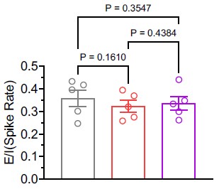
(2) The author should propose a potential mechanism for how TRPV3 helps to maintain cortical activity during fever. Would calcium influx-mediated change of membrane potential be the possible reason? Making a summary figure to put all the findings into perspective and propose a possible mechanism would also be appreciated.
Thank you for your helpful suggestion. In response, we have included a summary figure (Figure 11) illustrating the hypothesis described in the Discussion section. We agree with your assessment that Trpv3 most likely contributes to maintaining cortical activity during fever by promoting calcium influx and depolarizing the membrane potential.
(3) The author studied P7-8, P12-14, and P20-26 mice. How do these ages correspond to the human ages? it would be nice to provide a comparison to help the reader understand the context better.
Ideally, the mouse to human age comparison should depend on the specific process being studied. Per your suggestion, we have added additional references in the Introduction (Dobbing and Sands, 1973; Baram et al., 1997; Bender et al., 2004) to help readers better understand the correspondence between mouse and human ages.
Recommendations for the authors:
Reviewer #2 (Recommendations for the authors):
(3) Perform I-F curves to study the intrinsic properties of layer 2/3 neurons without the confound of evoked responses.
We performed F-I curve analyses (Figures 2H–I), as suggested by Reviewer 2, to study intrinsic properties of L2/3 neurons without evoked responses. Although rheobase increased at 39 °C compared to 30 °C, consistent with findings such as depolarized spike threshold and reduced input resistance, the mean number of spikes across current steps did not differ.
Reviewer #3 (Recommendations for the authors):
Some statistical descriptions are not clearly stated. For example, what statistical methods were used in Fig 2E? The effect size in Fig 2D seems to be quite small. The authors are advised to consider "nested analysis" to further increase the rigor of the analysis. Does each dot mean one neuron? Some of the data points might not be totally independent. The author should carefully check all figures to make sure the stats methods are provided for each panel.
We apologize for not including statistical details in Figure 2E. We have now added this information and verified that statistical descriptions are provided in all figure legends. In Figure 2D, each dot represents a cell, with measurements taken from the same cell at 30°C, 36°C, and 39°C. Given this design, the appropriate test is a one-way repeated-measures ANOVA.
Reviewer #3 (Public review):
Summary and Significance:
In this work, Cary and Hayashi address the important question of when, in evolution, certain mobile genetic elements (Ty3/gypsy-like non-LTR retrotransposons) associated with certain membrane fusion proteins (viral glycoprotein F or B-like proteins), which could allow these mobile genetic elements to be transferred between individual cells of a given host. It is debated in the literature whether the acquisition of membrane fusion proteins by non-LTR retrotransposons is a rather recent phenomenon that separately occurred in the ancestors of certain host species or whether the association with membrane fusion proteins is a much more ancient one, pre-dating the Cambrian explosion. Obviously, this question also touches upon the origin of the retroviruses, which can spread between individuals of a given host but seem restricted to vertebrates. Based on convincing data, Cary and Hayashi argue that an ancient association of non-LTR retrotransposons with membrane fusion proteins is most probable.
Strengths:
The authors take the smart approach to systematically retrieve apparently complete, intact, and recently functional Ty3/gypsy-like non-LTR retrotransposons that, next to their characteristic gag and pol genes, additionally carry sequences that are homologous to viral glycoprotein F (env-F) or viral glycoprotein B (env-B). They then construct and compare phylogenetic trees of the host species and individual encoded proteins and protein domains, where 3D-structure calculations and other features explain and corroborate the clustering within the phylogenetic trees. Congruence of phylogenetic trees and correlation of structural features is then taken as evidence for an infrequent recombination and a long-term co-evolution of the reverse transcriptase (encoded by the pol gene) and its respective putative membrane fusion gene (encoded by env-F or env-B). Importantly, the env-F and env-B containing retrotransposons do not form a monophyletic group among the Ty3/gypsy-like non-LTR retrotransposons, but are scattered throughout, supporting the idea of an originally ancient association followed by a random loss of env-F/env-B in individual branches of the tree (and rather rare re-associations via more recent recombinations).
Overall, this is valuable, stimulating, and important work of general and fundamental interest, but still also somewhat incompletely explored, imprecisely explained, and insufficiently put into context for a more general audience.
Weaknesses:
Some points that might be considered and clarified:
(1) Imprecise explanations, terms, and definitions:
It might help to add a 'definitions box' or similar to precisely explain how the authors decided to use certain terms in this manuscript, and then use these terms consistently and with precision.
a) In particular, these are terms such as 'vertebrate retrovirus' vs 'retrovirus' vs 'endogenized retrovirus' vs 'endogenous retrovirus' vs 'non-LTR retrotransposon' and 'Ty3/gypsi-like retrotransposon' vs 'Ty3/gypsy retrotransposon' vs 'errantivirus'.
b) The comment also applies to the term 'env' used for both 'env-F' and 'env-B', where often it remains unclear which of the two protein types the authors refer to. This is confusing, particularly in the methods, where the search for the respective homologs is described.
c) Other examples are the use of the entire pol gene vs. pol-RT for the definition of the Ty3/gypsy clade and for the generation of phylogenetic trees (Methods and Figure S1), and the names for various portions of pol that appear without prior definition or explanation (e.g., 'pro' in Figure 1A, 'bridge' in Figure S1C, 'the chromodomain' in the text and Figure 7).
d) It is unclear from the main text which portions of pol were chosen to define pol-RT and why. The methods name the 'palm-and-fingers', 'thumb', and 'connections' domains to define RT. In the main text, the 'connection' domain is called 'tether' and is instead defined as part of the 'bridge' region following RT, which is not part of RT.
(2) Insufficient broader context:
a) The introduction does not state what defines Ty3/gypsy non-LTR retrotransposons as compared to their closest relatives (Ty1/copia retrotransposons, BEL/pao retrotransposons, vertebrate retroviruses). This makes it difficult to judge the significance and generality of the findings.
b) The various known compositions of Ty3/gypsi-like retrotransposons are not mentioned and explained in the introduction (open reading frames, (poly-)proteins and protein domains, and their variable arrangement, enzymatic activities, and putative functions), and the distribution of Ty3/gypsi-like retrotransposons among eukaryotes remains unclear. The introduction does not mention that Ty3/gypsi-like retrotransposons apparently are absent from vertebrates, and Figure 7 is not very clear about whether or not it includes sequences from plants ('Chromoviridae').
c) The known association of Ty3/gypsi-like retrotransposons from different metazoan phyla with putative membrane fusion proteins (env-like) genes is mentioned in the introduction, but literature information, whether such associations also occur in the context of other retrotransposons (e.g., Ty1/ copia or BEL/pao), is not provided. The abstract is somewhat misleading in this respect. Finally, the different known types of env-like genes are not mentioned and explained as part of the introduction ('env-f', 'env-B', 'retroviral env', others?)
d) Some key references and reviews might be added:
- Pelisson, A. et al. (1994) https://www.embopress.org/doi/abs/10.1002/j.1460-2075.1994.tb06760.x<br /> (next to Song et al. (1994), for the identification of env in Ty3/gypsy)
- Boeke, J.D. et al. (1999)<br /> In Virus Taxonomy: ICTV VIIth report. (ed. F.A. Murphy),. Springer-Verlag, New York.<br /> (cited by Malik et al. (2000) - for the definition and first use of the term 'errantivirus')
- Eickbush, T.H. and Jamburuthugoda, V.K. (2008) https://doi.org/10.1016/j.virusres.2007.12.010<br /> (on the classification of retrotransposons and their env-like genes)
- Hayward, A. (2017) https://doi.org/10.1016/j.coviro.2017.06.006<br /> (on scenarios of env acquisition)
(3) Incomplete analysis:
a) Mobile genetic elements are sometimes difficult to assemble correctly from short-read sequencing data. Did the authors confirm some of their newly identified elements by e.g., PCR analysis or re-identification in long-read sequencing data?
b) The authors mention somewhat on the side that there are Ty3/gypsy elements with a different arrangement (gag-env-pol instead of gag-pol-env). Why was this important feature apparently not used and correlated in the analysis? How does it map on the RT phylogenetic tree? Which type of env is found with either arrangement? Is there evidence for a loss of env also in the case of gag-env-pol elements?
c) Sankey plots are insufficiently explained. How would inconsistencies between trees (recombinations) show up here? Why is there no Sankey plot for the analysis of env-B in Figure 5?
d) Why are there no trees generated for env-F and env-B like proteins, including closely related homologous sequences that do NOT come from Ty3/gypsy retrotransposons (e.g., from the eukaryotic hosts, from other types of retrotransposons (Ty1/copia or BEL/pao), from viruses such as Herpesvirus and Baculovirus)? It would be informative whether the sequences from Ty3/gypsy cluster together in this case.
e) Did the authors identify any other env-like ORFs (apart from env-F and env-B) among Ty3/gypsy retrotransposons? Did they identify other, non-env-like ORFs that might help in the analysis? It is not quite clear from the methods if the searches for env-F and env-B - containing Ty3/gypsy elements were done separately and consecutively or somehow combined (the authors generally use 'env', and it is not clear which type of protein this refers to).
f) Why was the gag protein apparently not used to support the analysis? Are there different, unrelated types of gag among non-LTR retrotransposons? Does gag follow or break the pattern of co-evolution between RT and env-F/env-B?
g) Data availability. The link given in the paper does not seem to work (https://github.com/RippeiHayashi/errantiviruses_2025/tree/main). It would be useful for the community to have the sequences of the newly identified Ty3/gypsy retrotransposons listed readily available (not just genome coordinates as in table S1), together with the respective annotations of ORFs and features.
4), African American andCaucasian primary-school children were presented with sentenceimitation and comprehension tasks. The African Americanchildren's ability to perform these tasks was taken to indicate anabsence of comprehension difficulty across vari
AA children were considered to have less comprehension of the language
islamophobie et génocide
Il semble manquer un déterminant pour chaque terme :
"...sur l'islamophobie et le génocide".
Il est aussi possible de nuancer le propos ainsi :
"...sur la question / l'enjeu / le concept de l'islamophobie et du génocide"
sont susceptibles de jure d’être de la sorte justifiées par un élément cognitif
"de jure" semble un peu éloigné de l'élément qu'il qualifie. Je proposerais de les rapprocher pour éclaircir le sens :
"...sont susceptibles d'être de la sorte justifiées de jure par un élément cognitif"
OU
"...sont de jure susceptibles d'être de la sorte justifiées par un élément cognitif"
Briefing : Le Rôle des Modèles dans le Développement de l'Enfant
Ce document de synthèse analyse le rôle complexe et multifacette des modèles dans le développement de l'enfant, en se basant sur les perspectives de psychologues, d'experts en développement et de témoignages personnels.
Il ressort que les parents constituent les modèles les plus fondamentaux, dont l'influence est primordiale durant les premières années.
Cependant, la recherche de la perfection parentale est contre-productive ; l'authenticité, la capacité à reconnaître ses erreurs et à s'excuser sont bien plus formatrices.
L'enfant n'imite pas aveuglément mais opère une sélection rigoureuse de ses modèles, privilégiant la compétence, la familiarité et la confiance.
Les modèles parentaux dysfonctionnels, marqués par l'addiction ou des troubles psychiques, ont des conséquences graves et durables sur la sécurité affective et l'estime de soi de l'enfant.
À l'adolescence, la recherche de modèles s'élargit au-delà du cercle familial pour construire une identité propre, un processus sain de différenciation qui peut inclure la rébellion et l'adhésion à des groupes de pairs.
Enfin, une perspective émergente et cruciale est mise en lumière : les enfants et adolescents ne sont pas de simples récepteurs passifs mais peuvent être de puissants modèles et des acteurs de changement, capables d'influencer positivement leur entourage, y compris leurs propres parents, et de façonner la société de demain.
--------------------------------------------------------------------------------
Le processus par lequel un enfant choisit et imite un modèle est loin d'être passif.
Il repose sur des mécanismes neurologiques et psychologiques complexes qui démontrent une grande sélectivité dès le plus jeune âge.
• Bases Neurologiques : Selon Moritz Köster, professeur de psychologie du développement, lorsqu'un enfant observe quelqu'un agir, des séquences de mouvements similaires sont activées dans son propre cortex moteur au niveau cellulaire.
• Sélectivité Basée sur la Confiance : L'enfant n'imite pas tout ce qu'il voit. Son choix est nuancé par les émotions et une évaluation de la personne observée. Les principaux critères de sélection sont :
◦ La familiarité : Il préférera imiter une personne qu'il connaît.
◦ La compétence : Il analyse si la personne a déjà fait des choses "intelligentes" ou des erreurs, et choisira d'imiter la personne jugée la plus compétente.
◦ L'autorité : Pour tout ce qui est nouveau, l'enfant se tournera préférentiellement vers les adultes, qu'il perçoit comme des figures de confiance.
• Apprentissage des Normes : C'est principalement en observant le comportement des adultes et de leur entourage que les enfants apprennent et intègrent les valeurs et les normes sociales.
Lise, 8 ans : "Pour moi un modèle c'est quand on fait quelque chose de bien et que quelqu'un d'autre nous imite."
L'environnement familial, et plus particulièrement les parents, constitue la première et la plus puissante source de modèles pour un enfant, une influence que les parents ont souvent tendance à sous-estimer.
Durant les premières années de vie (1-2 ans), l'environnement de l'enfant est restreint aux parents et grands-parents.
Leur comportement façonne entièrement la compréhension initiale de l'enfant sur les interactions sociales.
• Apprentissage des Comportements Sociaux : La manière de gérer un conflit, d'éviter les disputes ou de présenter des excuses est directement apprise par l'observation des parents.
• Ancrage Émotionnel : Si les échanges familiaux sont marqués par la bienveillance et l'amour, l'enfant intègre ce modèle. Inversement, si les cris ou la violence sont la norme, il retiendra ce schéma comme référence.
• La Famille comme Microcosme : Au départ, l'enfant perçoit le monde entier comme fonctionnant selon les règles de sa propre famille. Ce n'est qu'à son entrée en maternelle qu'il découvre la diversité des modes de fonctionnement.
La psychologue Nora Imlau met en garde contre la volonté de certains parents de devenir "parfaits" après la naissance d'un enfant, la qualifiant de "très mauvaise idée".
• L'Inauthenticité : Les enfants ressentent très bien quand leurs parents ne sont pas authentiques, se mettent la pression et ignorent leurs propres besoins.
• Un Standard Inatteignable : Un enfant confronté à des modèles "parfaits" (qui ne se mettent jamais en colère, ne perdent jamais patience) n'a aucune chance de faire aussi bien.
Il sera sans cesse confronté à ses propres insuffisances.
• L'Importance de l'Erreur : Le fait que les parents commettent des erreurs est une opportunité d'apprentissage cruciale.
Cela permet à l'enfant d'apprendre comment on gère ses propres erreurs.
Présenter ses excuses à ses enfants pour des propos qui ont "dépassé notre pensée" est un acte modelant très puissant.
Nora Imlau, psychologue : "Ce que j'entends par parents parfaits, ce sont les parents qui ne se mettent jamais en colère, qui ne perdent jamais patience [...] ce qui est inhumain en soi."
Le comportement d'un enfant est souvent le reflet de l'état d'âme inconscient de ses parents. Un enfant agité peut être le miroir d'un parent stressé ou préoccupé.
• La Gestion de la Tristesse : Quand un parent est triste et qu'un enfant vient le consoler, il est conseillé d'accepter cette aide dans un premier temps.
Cependant, il est crucial que le parent reprenne ensuite le contrôle et rassure l'enfant sur sa capacité à gérer la situation, afin de ne pas inverser les rôles et de préserver l'enfant de la charge de ses responsabilités d'adulte.
• La Vulnérabilité Assumée : Une mère souffrant de trouble bipolaire témoigne de sa capacité à être présente pour ses enfants même dans les phases de dépression, tout en ne cachant pas sa tristesse.
Cela illustre la possibilité de rester un parent fonctionnel malgré des difficultés psychiques.
Lorsque les parents ne peuvent pas s'occuper correctement de leurs enfants, que ce soit à cause d'une dépendance ou d'un trouble psychique, les conséquences sur le développement de l'enfant sont multiples et profondes.
Le témoignage de Mia, 16 ans, dont le père était alcoolique, illustre les dégâts d'un modèle parental défaillant.
• Rupture de la Confiance : Un parent souffrant de dépression ou d'addiction n'est plus en mesure d'interpréter correctement les signaux de son enfant et d'y réagir de manière adaptée.
L'enfant retient que ses besoins ne sont pas satisfaits.
• Attachement Insécurisant : La relation d'attachement parent-enfant ne devient pas sécurisante, ce qui entrave la construction de la confiance en soi.
Cette confiance initiale est pourtant la base essentielle du développement de l'autonomie.
• Hypervigilance de l'Enfant : L'enfant est constamment aux aguets, utilisant une énergie considérable pour anticiper les réactions de ses parents et adapter son propre comportement, ce qui peut entraîner des problèmes d'autonomie et de sentiment de sécurité à l'âge adulte.
Mia, 16 ans : "En fait il fallait toujours qu'on soit la famille parfaite, on parlait jamais des problèmes, on avait pas le droit d'en parler et ça c'est très mal."
Suite à la séparation de ses parents et à ses propres difficultés psychologiques, Mia a été confrontée à des "modèles toxiques" dans un cadre thérapeutique.
• Influence des Pairs : En observant des jeunes toxicodépendants, elle a perçu leur consommation comme un moyen de "déconnecter totalement" et de ne plus être accessible émotionnellement, un état qu'elle a alors désiré atteindre.
• Augmentation de la Consommation : Son exposition à ces modèles a directement influencé son propre comportement, entraînant une augmentation significative de sa consommation d'alcool.
L'adolescence est une période de questionnements identitaires intenses ("Qui suis-je ?") où la recherche de modèles s'intensifie et s'étend au-delà du cercle familial.
Selon la psychothérapeute Isabelle Filliozat, l'adolescent va "chercher des modèles un petit peu partout pour [s]'aider à se construire".
• Le Rôle du Groupe : Le désir d'appartenance à un groupe de pairs est très fort.
Le groupe offre un cadre identitaire ("dans mon groupe on fait les choses d'une certaine manière [...] je sais à peu près qui je suis").
• Gestion des Modèles Négatifs : Lorsqu'un enfant adhère à un modèle jugé "malsain" (agressif, délinquant), la réaction parentale la plus constructive n'est pas de chercher à changer le comportement extérieur, mais de s'intéresser aux besoins et aux émotions de l'enfant qui le poussent vers ce modèle.
En répondant à ces besoins profonds, l'enfant est plus susceptible d'abandonner de lui-même le modèle négatif.
La révolte contre les parents à l'adolescence est un processus "sain et normal", une étape nécessaire du développement.
• Processus de Détachement : Les frictions parents-enfants font partie du processus de détachement et de la prise de conscience par l'adolescent qu'il est une personne à part entière, distincte de ses parents.
• Différenciation : Pour se construire, l'adolescent a besoin de s'opposer, de définir en quoi il est différent de ses parents (valeurs, mentalité) mais aussi en quoi il leur ressemble.
Ce processus est essentiel pour pouvoir, à terme, quitter le foyer et construire une nouvelle relation, d'adulte à adulte, avec ses parents.
La vision traditionnelle du modèle descendant (adulte vers enfant) est de plus en plus complétée par une reconnaissance du rôle actif des jeunes comme modèles et agents d'influence.
Des recherches ont démontré que les enfants peuvent avoir une influence positive sur la manière de penser et sur le comportement de leurs parents.
• "L'Hypothèse des Anniversaires" : Dans des zones post-conflit, le fait que des enfants d'un groupe ethnique ou religieux invitent à leur anniversaire des enfants d'un groupe adverse force les parents des deux bords à entrer en contact.
Il a été observé que lorsque l'attitude des enfants envers "l'autre groupe" change, celle des parents change également.
• Acteurs de Paix : Les enfants peuvent ainsi devenir des acteurs clés de la promotion de la paix.
Des adolescents comme Noé Renard, 17 ans, s'imposent comme des modèles d'engagement pour leur génération.
• Rendre l'Engagement Accessible : En créant l'association "les engagés Marseille", son but est de montrer l'exemple et de permettre à d'autres jeunes de se mobiliser sur des enjeux locaux (inégalités, pollution, mobilité).
• Une Voix pour la Jeunesse : De nombreux jeunes partagent le sentiment de ne pas être suffisamment écoutés dans les institutions politiques.
Ils peuvent devenir des modèles pour leurs pairs mais aussi pour les chercheurs, comme l'illustre la mise en place d'un Conseil consultatif de la jeunesse à l'Université libre de Berlin.
Noé Renard, 17 ans : "Défendre des causes c'est pas le faire pour soi mais c'est plutôt le faire pour les autres et je pense que c'est ça qui est important c'est de pouvoir montrer aux autres que l'engagement c'est [...] surtout pour les autres et pour aider ceux qui en ont besoin."
Une critique est formulée quant au fait d'attendre la majorité pour accorder le droit de vote sans formation préalable aux règles de la démocratie.
• Apprentissage Précoce : Les experts plaident pour que les enfants apprennent beaucoup plus tôt comment fonctionne un consensus, comment on règle les conflits dans une démocratie, et qu'ils aient davantage d'influence sur leur vie quotidienne.
• Faire Confiance : Pour que les jeunes développent leur identité et leur capacité à prendre des responsabilités, les parents doivent apprendre à leur faire confiance et à les laisser expérimenter par eux-mêmes, même si c'est "à leur façon".
L’étude The World Unplugged a demandé à un millier d’étudiants provenant d’une douzaine d’universités des cinq continents, de faire l’expérience de 24h de déconnexion médiatique (Moeller et al., 2012). Les résultats ont été univoques : une nette majorité d’étudiants a admis l’échec pur et simple de leurs efforts de déconnection. Beaucoup d’entre eux se sont alors auto-déclarés « addicts » aux médias et technologies de communication numérique.
Argument pour : les résultats de cette étude, pourtant mondiale, ont indiqué que la majorité des étudiants n'ont pas réussi à déconnecter, ne serait-ce que 24h, et se sont même considérés comme dépendants. Ceci évoque un comportement proche d’un processus addictif (désir incontrôlable, auto-déclaration d’addiction).
Cependant, de telles pratiques ne constituent pas une réelle dépendance au sens pathologique car elles ne sont pas de nature compulsive.
Argument contre : dans l'addiction, on note une conduite compulsive, mais ici, l’usage excessif est expliqué par la compensation de besoins sociaux.
Cependant, les internautes qui les fréquentent intensivement ont davantage tendance à effectuer des comparaisons sociales dont les résultats sont en leur défaveur (Lee, 2014). Ils sont aussi enclins à penser que les autres sont plus heureux et ont une vie bien plus agréable que la leur, ce qui leur donne un sentiment d’injustice (Chou, Edge, 2012). Ce biais conduit au déclenchement de certains processus psychopathologiques, comme des ruminations mentales
Argument contre : le texte montre que les effets négatifs d'une fréquentation intense d'internet (dépression, anxiété) sont liés à des comparaisons sociales et à des ruminations, des pensées négatives, mais pas à une dépendance.
le désir d’utiliser les médias (consulter ses e-mails, surfer sur le Web, aller sur les RSN, regarder la télévision) est celui pour lequel notre capacité de résister serait la plus faible. Non seulement le désir d’utiliser les médias serait plus fort et plus fréquent dans une journée que, par exemple, le désir de tabac, mais il serait, en outre, plus difficile à contrôler que les désirs de manger ou d’avoir des activités sexuelles
Argument pour : La difficulté à résister à un usage numérique fait état d'impulsions généralement associées aux addictions comportementales.
L’addiction à Internet ne figure pas dans la dernière version du Manuel diagnostique et statistique des troubles mentaux (DSM 5 ; APA, 2015) manuel de référence internationale pour la plupart des psychiatres et psychologues. À l’excès, ces habitudes sont étiquetées « comportements excessifs », mais ne sont pas définies comme de véritables troubles mentaux en raison, actuellement, de l’insuffisance de données dans la littérature (DSM 5 ; APA, 2015, p. 571).
Argument contre : l'addiction à internet est plutôt vue comme une pratique excessive que comme un véritable trouble mental. En tout cas, elle n'est pas reconnue par le DSM 5, on ne cite pas ici par exemple de critères cliniques.
Exncon:
klais kai klais kai klais kai epeidh den sou dinei kanenas shmasia stamatas na klais
Nous mettrons plus précisément en évidence les nombreux facteurs indiquant que les thérapies basées sur Internet constituent, cent ans après la naissance de la discipline, un défi profond et durable à la psychothérapie.
Argument pour : à travers la notion de défi indiquée, internet peut-il donc influencer les comportements des individus ?
La brièveté des contacts avec ce dernier répond alors à un objectif important, expliqué précédemment : pour pouvoir augmenter l’accessibilité d’un traitement, il faut qu’un même professionnel puisse s’occuper de plus de patients.
Argument contre : internet permet donc d'optimiser les ressources, en permettant à davantage de patient d'avoir accès à un professionnel.
La thérapie, ou plus précisément le changement thérapeutique, n’est plus assurée par un thérapeute mais par un programme de self-help, et le rôle de thérapeute n’est que de faciliter le suivi du programme.
Argument pour : les usages numériques ne pourraient-ils alors pas engendrer une fragilité possible, créant un terrain propice à des comportements inappropriés ?
L’objectif principal de cette deuxième démarche consiste à augmenter l’accessibilité de la psychothérapie, c’est-à-dire réduire les obstacles que peuvent rencontrer les patients lorsqu’ils souhaitent faire appel à un dispositif de soin. Cette question constitue un défi majeur pour de très nombreux systèmes de soins nationaux (Richards, Lovell & McEvoy, 2003). La seule manière pour une personne d’avoir accès à une thérapie traditionnelle est souvent de recourir à un thérapeute exerçant dans le secteur privé. Cela n’est cependant possible que pour des individus disposant de ressources économiques relativement importantes. Or, l’accessibilité s’améliore avec les programmes de self-help, dans la mesure où ces derniers rendent la thérapie moins dépendante de la disponibilité des thérapeutes : en diminuant le temps que consacre chaque thérapeute à chaque patient, un plus grand nombre de patients peuvent accéder à un traitement (Andersson, 2009).
Argument contre : cette position contredit l’idée que l'usage d'internet est nécessairement dangereux ou addictif : plusieurs arguments sont développés ici (accessibilité, disponibilité, possibilités financières …)
depuis environ dix ans, Internet est également envisagé comme un espace où peuvent se pratiquer la psychothérapie et le traitement psychologiqu
Argument contre : ici internet peut être envisagé comme un outil de soin, pas seulement un espace de risque.
Le terme de pratique excessive (et a fortiori d’addiction) fait intervenir la notion de retentissement durable sur la vie du sujet : perturbations du sommeil, troubles du comportement alimentaire (surpoids, grignotage), absentéisme et/ou échec scolaire, retrait social, diminution des autres activités (familiales, sportives et culturelles).
Argument pour : même si on parle ici d'addiction "a fortiori", les critères de dépendance décrits y ressemblent fortement.
Il n’y a pas de consensus scientifique sur l’existence de réelles addictions aux jeux vidéo. En l’absence d’études précisant leurs critères, il est préférable d’utiliser le terme de pratiques excessives
Argument contre : la notion d’addiction numérique reste controversée.
L’accès à ces jeux suscite des craintes du fait du risque de pratique excessive. Certains utilisent même le terme d’addiction, définie comme la perte de contrôle et la poursuite du comportement malgré ses conséquences négatives
Argument pour : le vocabulaire de l’addiction est ici utilisé pour les activités numériques.
Écologie : Complexité, Paradoxes et Holisme — Synthèse de la Leçon Inaugurale de Franck Courchamp
Cette note de synthèse résume la leçon inaugurale de Franck Courchamp, titulaire de la chaire annuelle "Biodiversité et écosystèmes" au Collège de France.
La présentation articule l'étude de l'écologie autour de trois concepts fondamentaux : la complexité, les paradoxes et le holisme.
Franck Courchamp, directeur de recherche au CNRS et scientifique de renommée mondiale, démontre que la biodiversité est un système d'une richesse et d'une interconnexion extraordinaires, dont la compréhension ne peut être que partielle sans une approche globale.
Les points clés sont les suivants :
• La Biodiversité est une réalité multidimensionnelle et largement méconnue.
Définie à trois niveaux (spécifique, génétique, écosystémique), elle représente une richesse quantitative (potentiellement jusqu'à 10 milliards d'espèces de procaryotes) et qualitative (valeur utilitaire et intrinsèque) immense.
Cependant, la science n'a décrit qu'une infime fraction de cette diversité (2,3 millions d'espèces eucaryotes), alors même qu'un million d'espèces sont menacées d'extinction.
• La complexité est la caractéristique fondamentale des écosystèmes.
Le nombre vertigineux d'espèces (des dizaines de milliers dans une surface équivalente à une salle de conférence en forêt amazonienne) et la multitude d'interactions directes et indirectes entre elles et avec leur environnement créent des systèmes dynamiques et auto-organisés d'une complexité qui dépasse souvent l'intuition.
• De cette complexité naissent des paradoxes écologiques. De nombreux phénomènes observés en écologie sont contre-intuitifs.
Par exemple, l'ajout d'engrais peut appauvrir la diversité végétale, la prévention des incendies peut engendrer des méga-feux, et la réintroduction de prédateurs comme le loup peut paradoxalement rendre les routes plus sûres en modifiant le comportement de leurs proies.
• L'approche holistique est indispensable pour comprendre et agir.
Seule une vision globale de l'écosystème, intégrant toutes ses composantes et interactions, permet de déchiffrer ces paradoxes et d'éviter des interventions de conservation aux conséquences inverses de celles escomptées.
L'exemple de la réintroduction des loups à Yellowstone, qui a modifié jusqu'au cours des rivières, illustre parfaitement la puissance des effets en cascade qu'une approche holistique peut révéler.
La conférence conclut que ces trois concepts — complexité, paradoxes, holisme — sont des outils intellectuels essentiels pour naviguer dans le champ de l'écologie.
Ils formeront le fil conducteur des cours à venir, qui se concentreront sur la biologie des invasions, en adoptant une perspective résolument interdisciplinaire.
--------------------------------------------------------------------------------
La leçon inaugurale a été prononcée dans le cadre de la cinquième édition de la chaire annuelle "Biodiversité et écosystèmes" du Collège de France, une initiative soutenue par la Fondation Jean-François de Clermont-Tonnerre.
Cette chaire vise à promouvoir la recherche et à éclairer le débat public sur les enjeux du vivant.
Le titulaire de la chaire, Franck Courchamp, est une figure de premier plan dans le domaine de l'écologie. Ses qualifications incluent :
• Positions académiques : Directeur de recherche première classe au CNRS, il dirige une équipe à l'Université Paris-Saclay et est titulaire de la chaire AXA "Biologie des invasions".
• Reconnaissance internationale : Auteur de plus de 200 publications, il est l'un des scientifiques les plus cités au monde dans son domaine et contribue aux travaux de panels intergouvernementaux majeurs comme le GIEC et l'IPBES.
• Distinctions : Il a reçu de nombreuses récompenses, dont la médaille d'argent du CNRS (2011), a été nommé à l'Académie européenne des sciences (2014) et fait chevalier de l'Ordre national du Mérite (2021).
• Vulgarisation : Reconnu pour son talent de communicant, il a participé à des documentaires (notamment la série Une espèce à part sur Arte), et a publié des ouvrages grand public tels que L'Écologie pour les nuls et la bande dessinée La Guerre des fourmis.
La biodiversité, contraction de "diversité biologique", est classiquement analysée selon trois échelles interdépendantes :
1. La biodiversité spécifique : Le nombre d'espèces présentes dans un espace donné (ex. : 160 000 à 180 000 espèces de papillons dans le monde). C'est le niveau le plus couramment étudié.
2. La biodiversité génétique : La diversité au sein d'une même espèce (ex. : les 340 races de chiens). Une faible diversité génétique, comme chez le guépard, rend une espèce très vulnérable.
3. La biodiversité écosystémique : La variété des écosystèmes dans un paysage (ex. : un paysage avec forêt, lac et prairie a une plus grande diversité écosystémique qu'un récif corallien, même si ce dernier a une très grande diversité spécifique).
L'ampleur de la biodiversité sur Terre reste largement sous-estimée.
• Espèces décrites : La science a formellement décrit 2,3 millions d'espèces eucaryotes (animaux, plantes, champignons, protistes).
• Espèces inconnues : Les estimations suggèrent que la grande majorité des espèces reste à découvrir. Le tableau suivant, évoqué dans la conférence, illustre ce déficit de connaissance :
Pourcentage d'Espèces Inconnues (estimation)
Mammifères
Près de 10 %
Poissons
Près de 90 %
Insectes
Près de 90 %
Algues
Près de 90 %
Champignons
Plus de 90 %
Franck Courchamp souligne : "Nous vivons, sans le savoir, dans un monde de champignons et d'insectes."
De plus, les eucaryotes ne sont qu'une infime partie du vivant ; les procaryotes (bactéries et archées) pourraient représenter jusqu'à 10 milliards d'espèces.
La biodiversité est importante pour l'humanité de deux manières distinctes :
• La valeur utilitaire : Elle fournit des "biens" et des "services" essentiels.
◦ Biens : Alimentation (seulement 12 espèces végétales fournissent 75% de la nourriture mondiale), matériaux (bois, coton, laine), et médicaments (deux tiers des molécules pharmaceutiques proviennent directement des plantes).
◦ Services : Pollinisation (près de 80% de nos cultures), purification de l'eau et de l'air, fertilisation des sols et biodégradation.
• La valeur intrinsèque : Chaque espèce, écosystème ou individu possède une valeur propre, indépendamment de son utilité pour l'être humain.
Une Richesse Menacée
Cette richesse est en péril. Le rapport de l'IPBES de 2019 a établi qu'un million d'espèces animales et végétales sont menacées d'extinction au cours des prochaines décennies, avec une accélération notable du rythme des extinctions récentes.
L'écologie est la discipline scientifique qui étudie les interactions entre les organismes et leur environnement. Elle est intrinsèquement liée à la science de l'évolution. Comme le formule Franck Courchamp : "L'écologie observe la danse des espèces dans leur environnement [...]. L'évolution raconte l'histoire de cette danse."
L'écologie analyse des systèmes à différentes échelles, des individus à la biosphère. L'étude de la dynamique des populations offre une porte d'entrée.
L'exemple classique des cycles prédateur-proie entre le lynx et le lièvre arctique, documenté grâce aux registres de la Compagnie de la Baie d'Hudson, montre comment des modèles mathématiques simples (comme le modèle de Lotka-Volterra) peuvent décrire des dynamiques complexes.
Cependant, la réalité est celle de réseaux trophiques où chaque espèce interagit avec de nombreuses autres, créant des systèmes d'une complexité immense, auxquels s'ajoutent les interactions non-vivantes (cycles biogéochimiques du carbone, de l'azote, etc.).
Franck Courchamp propose une grille de lecture de l'écologie fondée sur trois concepts interdépendants.
La biodiversité est un système caractérisé par une richesse, une dynamicité et un nombre d'interactions extraordinairement élevés.
Un exercice de pensée illustre ce point : sur une surface équivalente à celle de la salle de conférence, une forêt amazonienne peut abriter entre 10 000 et 20 000 espèces différentes, dont 5 000 à 10 000 espèces d'insectes.
L'ensemble des interactions directes et indirectes entre ces milliers d'acteurs forme un système dynamique, auto-organisé (autopoïétique) et multiscalaire.
De cette complexité émergent des résultats qui défient l'intuition. Ces paradoxes sont omniprésents en écologie.
• Paradoxes généraux :
◦ Écologie des communautés : L'ajout d'engrais peut "tuer" les plantes en favorisant quelques espèces dominantes au détriment de la diversité globale, rendant l'écosystème moins stable.
◦ Écologie forestière : La suppression systématique des feux de faible intensité mène à l'accumulation de combustible et à des "méga-feux" dévastateurs.
◦ Biologie de la conservation : Le retour des loups dans certaines régions des États-Unis a réduit de près d'un quart les accidents de voiture impliquant des cerfs, non pas en diminuant leur population, mais en modifiant leur comportement (création d'un "paysage de la peur").
• Paradoxes issus des recherches de Franck Courchamp :
◦ Épidémiologie : Les chats infectés par le VIF (sida du chat) vivent plus longtemps, car le virus se transmet lors de combats entre les individus les plus dominants et les plus robustes.
◦ Effet Allee : Pour certaines espèces sociales (suricates, lycaons), c'est l'incapacité à coopérer en dessous d'un certain seuil d'effectif qui cause l'extinction, et non la compétition.
◦ Paradoxe de la rareté : La rareté d'une espèce augmente sa valeur sur le marché (chasse, collection), ce qui intensifie son exploitation et accélère sa disparition dans une boucle de rétroaction positive.
◦ Espèces charismatiques : Elles sont à la fois les plus aimées, les plus menacées, et leur omniprésence culturelle nous fait croire à tort qu'elles sont communes, ce qui freine les efforts de conservation.
La clé pour comprendre ces paradoxes et agir efficacement est l'adoption d'une approche holistique, qui considère l'écosystème dans son ensemble.
• Pour Comprendre : L'Exemple des Loups à Yellowstone La réintroduction du loup, un prédateur apical, a déclenché une cascade d'effets dans tout l'écosystème :
1. Contrôle des élans : Diminution de la pression de broutage sur la végétation.
2. Régénération de la végétation : Les saules et les peupliers ont pu repousser.
3. Retour des castors : Avec plus de bois, les populations de castors ont explosé, créant des barrages.
4. Modification des rivières : Les barrages ont modifié l'hydrologie et la morphologie des cours d'eau, créant des habitats pour d'autres espèces (poissons, amphibiens, oiseaux). Cet exemple montre qu'une seule action peut avoir des répercussions profondes et inattendues sur l'ensemble du système.
• Pour Agir : Biologie de la Conservation Une vision non-holistique peut mener à l'échec. La surprotection des éléphants dans certaines réserves, sans tenir compte du reste de l'écosystème, a conduit à la dégradation de la végétation et a nui à d'autres herbivores.
De même, l'interdiction totale du commerce de l'ivoire, bien qu'intentionnée, a créé un marché noir qui a pu intensifier le braconnage dans certaines zones.
La complexité, les paradoxes et le holisme ne sont pas de simples concepts académiques, mais des outils essentiels pour déchiffrer le fonctionnement du vivant et orienter l'action humaine.
Ces principes formeront la structure des cours à venir de Franck Courchamp, qui se concentreront sur la biologie des invasions.
Chaque cours sera enrichi par un séminaire mené par un spécialiste d'une autre discipline (économie, philosophie, épidémiologie, etc.), soulignant la nécessité d'une approche interdisciplinaire pour relever les défis environnementaux actuels.
La leçon se termine sur une citation de Carl Sagan, rappelant que la nature recèle encore d'innombrables merveilles à découvrir : "Quelque part, quelque chose d'incroyable attend d'être connu."
You and 7 others reacted
Ka wai ola a Kāne
La parola kānaka maoli per indicare l'acqua è wai, mentre quella hawaiana per indicare la ricchezza è waiwai, a indicare che l'acqua è fonte di benessere e ricchezza
yam-hills
La coltivazione dell'igname in Giamaica utilizza il metodo dello “stick” (bastone), con materiale di piantagione chiamato “yam heads” (teste di igname) sepolto in singoli cumuli di terra chiamati “yam hills” (collinette di igname).
sans professionel ni compétences techniques requises
pas besoin d'être un pro, WALL_ter est à la portée de tous
Mettre plus en forme les section « en savoir plus » parce que la c’est un bloc de texte assez indigeste. Scinder en paragraphe et donner plus de forme au texte
Cette expertise est notre valeur ajoutée.
Peut être pas la meilleure formule possible
Gracias a diferentes equipos de fanes Xenogears se vio traducido al español después de varios años con más fidelidad a la versión japonesa, por supuesto, al ser solo por y para fanes, este no vio su salida en las tiendas. A través de la página web de los últimos autores se pueden descargar los parches para modificar los backups de los juegos originales y traducir incluso las cinemáticas de este.
New to me!
If the relationship between pressure and altitude were exactly exponential, this plot would be a straight line. It is not quite straight because the temperature of the atmosphere also comes into play, and temperature is also not constant with height. Pressure decreases with altitude less quickly where the atmosphere is warmer because the density is lower, and more quickly where the temperature is lower. However, these variations are not huge because the temperature range (in kelvin) is not large – about 213–288 K over the troposphere, for example – compared to pressure changes that span many orders of magnitude. We will look at temperature changes with altitude next.
pressure and altitude aren't exactly exponential because temperature has na impact Pressure decreases when the atmosphere is warmer as the density is lower, and increases when the temperature is lower as the density is higher These variations aren't huge because the temp range in kelvin is small, about 213-288K over the troposphere
hat reduction involves donating electrons in chemical reactions, and oxidation involves accepting electrons. Reducing gases are hydrogen or hydrogen-containing gases, such as methane (CH4), ammonia (NH3) and hydrogen sulfide (H2S). Oxidising gases include oxygen, ozone (O3) and other oxygen-containing gases. Essentially, this has meant going from an atmosphere free of oxygen to the current level of 21%. Consequently, we can infer what past atmospheres were like, as these changes have been recorded in rocks and sediments through chemical reactions between the atmosphere and the Earth’s crust, and biological processes associated with life. These stratigraphic records (layers in the Earth’s crust) have led to the division of geological time into four eons, each lasting hundreds of millions to billions of years: the Hadean Eon (4.6–4.0 billion years ago, bya), the Archean Eon (4.0–2.5 bya), the Proterozoic Eon (2.5 bya–540 million years ago, mya) and the Phanerozoic Eon (540 mya–now).
Reduction is donating electrons Oxidation is accepting electrons Reducing gases are hydrogen or contain hydrogen (methane, ammonia) Oxidising gases include oxygen We can see past atmospheres through records in rocks and seidements this has led to division of geological time into four eons: Haden 4.6-4 billion, Archea 4-2.5, Proterozic 2.5-540 and Phanerozoic
Il vaccino contro il meningococco B ha fatto risparmiare € 38 759 608. Per i soggetti vaccinati si stima una efficacia dell'87%. Il vaccino contro il rotavirus ha fatto risparmiare € 26 687 952. Per i soggetti vaccinati vi è una riduzione del 75% del rischio di incorrere in gastroenteriti ed ospedalizzazioni. La prevenzione della varicella infantile (vaccino somministrato in 2 dosi) ha fatto risparmiare € 23 300 000. In caso di copertura vaccinale della popolazione del 90% si riducono dell'87% i casi. Il vaccino contro il virus del papilloma umano nei maschi undicenni ha fatto risparmiare € 71 000 000. C'è stata una riduzione degli eventi HPV grazie ad una copertura vaccinale universale del 64%. Il vaccino contro lo pneumococco ha fatto risparmiare € 18 750 000. Negli anziani ha consentito di evitare oltre 5000 casi di polmonite non batteriemica pneumococcica (NBPP), più di 2500 casi di infezioni invasive da pneumococco (IPD), circa 3200 casi di meningite pneumococcica e circa 3300 sequele da infezioni pneumococciche. La prevenzione della varicella zoster (vaccino somministrato ad anziani) ha fatto risparmiare € 38 759 608. Sono stati evitati circa 9 724 casi di herpes zoster (HZ) e circa 898 casi di neuropatia post-herpetica (NPH).[
Dati palesemente falsi e non validati da nessuno studio scientifico N.B.: Il risparmio riportato per il vaccino meningococcico B e quello per la varicella zoster sono identici: € 38 759 608, il che è veramente ridicolo Credibilità = 0**
Per rendere le vaccinazioni più efficaci vengono stilate successioni cronologiche, riassunte nei cosiddetti "calendari vaccinali", predisposti dalle autorità sanitarie nazionali, e che riguardano principalmente le vaccinazioni in ambito pediatrico.
successioni cronologiche prive di fondamenta scientifiche e la cui validità è non dimostrata. La ripresa dell'incidenza di malattie gravi o potenzialmente mortali (che sarebbero facilmente evitabili tramite semplici vaccinazioni) è arbitraria e gratuita...
(sous la direction de Tony Gheeraert et en colaboration avec la Chaire d’excellence en édition numérique de l’Université de Rouen Normandie)
Je sais pas si j'ai déjà vu des notes de bas de page dans les proposition pour des colloques. La parenthèse probablement est mieux. Je rajouterais la collaboration avec le PURH.
Porreglageneralseprocedeprecisamentealainversa,viéndoseenlarelaciéndevalortansdlolaproporciénenqueseequiparandeterminadascantidadesdedosclasesdistintasdemercancias.Sepasaporalto,deestasuerte,quelasmagnitudesdecosas diferentesnolleganasercomparablescuantitativamentesinodespuésdesureducciéna lamismaunidad.Sloencuantoexpresio-nesdelamismaunidadsonmagnitudesdelamismadeno-minacién,yportantoconmensurables.™
Contendido de la forma relativa del valor, nos sugiere que debemos encontrar ese ALGO que nos permita transformar formas de trabajo diferentes, mercancías de diferente uso, cualitativamente, donde podamos equipararlas, cuantitativamente.
Por ello, si en lo que se refiere al valor de uso eltrabajo contenido en la mercancia sdlo cuenta cualitativa-mente, en lo que tiene que ver con la magnitud de valor,cuenta s6lo cuantitativamente, una vez que ese trabajo sehalla reducido a la condicién de trabajo humano sin mascualidad que ésa. Alli, se trataba del cémo y del qué deltrabajo; aqui del cudnto, de su duracién.
Aquí se nos esta introduciendo al hecho de como es posible equiparar dos mercancías que son cualitativamente diferentes. Es por medio de la medición de la duración del TRABAJO puesto a su creación. Mas abajo en breve se nos insiste que las mercancías en el solo representan la cantidad de trabajo en ella contenida (duración del trabajo util en ellas contenida).
RRID:AB_469228
DOI: 10.1016/j.xcrm.2025.102466
Resource: None
Curator: @scibot
SciCrunch record: RRID:AB_469228
RRID:AB_2869977
DOI: 10.1016/j.xcrm.2025.102466
Resource: (BD Biosciences Cat# 566967 (also 566968), RRID:AB_2869977)
Curator: @scibot
SciCrunch record: RRID:AB_2869977
L'Égalité des Genres : Analyse des Origines du Patriarcat et des Modèles Alternatifs
Ce document de synthèse analyse la thèse selon laquelle le patriarcat n'est pas une loi naturelle et immuable, mais une construction historique.
S'appuyant sur des exemples historiques, archéologiques et anthropologiques, il démontre que les relations entre les genres ont pris des formes très diverses au cours de l'histoire humaine.
L'égalité a non seulement existé, mais elle persiste dans certaines sociétés matrilinéaires contemporaines.
L'analyse révèle que l'émergence des premiers États a été un facteur décisif dans l'institutionnalisation et la propagation mondiale du patriarcat comme outil de contrôle démographique et social.
Le cas de l'Islande illustre que l'égalité moderne est une conquête récente et fragile, fruit d'une lutte collective déterminée, et non un retour à un état originel.
En conclusion, la reconnaissance de la mutabilité des structures sociales ouvre la voie à la possibilité de construire un avenir égalitaire, en comprenant que l'ordre social actuel n'est pas une fatalité.
--------------------------------------------------------------------------------
La perception commune présente la lutte pour les droits des femmes comme un combat sans fin contre un patriarcat qui serait une constante de l'histoire humaine. Cette vision postule une rébellion perpétuelle contre l'exclusion du pouvoir, le travail domestique non rémunéré et la violence.
Le documentaire remet fondamentalement en cause cette narration en posant la question centrale : « les femmes et les hommes n'ont-ils jamais été égaux ? ».
Il suggère que loin d'être une "loi naturelle", l'organisation patriarcale n'est qu'une des nombreuses façons dont les sociétés humaines ont structuré les relations de genre au fil du temps.
L'Islande est souvent citée comme un modèle de l'égalité des genres au 21e siècle, avec une égalité salariale inscrite dans la loi, un congé parental largement adopté par les pères, et des femmes aux plus hautes fonctions politiques. Cependant, cette situation est le résultat d'une lutte récente et intense.
• Le Contexte d'Inégalité : Dans les années 1970-80, la situation était radicalement différente.
L'anthropologue Sigridur Duna Christmunir, cofondatrice du premier parti féministe islandais en 1983, rapporte qu'à l'époque, les femmes gagnaient à peine 60 % du salaire de leurs collègues masculins.
Elle compare la frustration grandissante des femmes à une « éruption volcanique ».
• La Grève Historique du 24 octobre 1975 : Face à cette inégalité, 90 % des femmes islandaises ont refusé de travailler lors du « jour de vacances des femmes » (gena Frida Urine).
Cette grève concernait à la fois le travail rémunéré et les tâches domestiques (cuisine, garde d'enfants, ménage).
◦ Impact : La société a été « totalement paralysée », créant un « état d'urgence total ».
Sigridur Duna Christmunir se souvient :
« Je sentais l'odeur de la viande brûlée dans les rues. Les hommes faisaient la cuisine [...]. L'odeur de la viande brûlée me rappelle toujours cette journée. »
• Conséquences Politiques et Législatives : L'événement a provoqué une accélération spectaculaire des réformes :
◦ 1976 : Entrée en vigueur de la loi sur l'égalité salariale.
◦ 1980 : Élection de Vigdís Finnbogadóttir, première femme au monde élue présidente démocratiquement.
◦ Par la suite, l'entrée au parlement de la « Liste des femmes », dont faisait partie Sigridur Duna, a « révolutionné la politique islandaise ».
L'analyse historique et archéologique révèle des indices d'organisations sociales non patriarcales, contredisant l'idée d'une domination masculine universelle.
Les sagas et les découvertes archéologiques nuancent l'image d'une société viking strictement patriarcale.
• Droits et Autonomie : Les sagas du 13e siècle, comme la Saga de Laxdæla, dépeignent des femmes de la classe supérieure comme intelligentes et volontaires.
Le premier recueil de lois islandais, les Grágás, confirme que les femmes vikings pouvaient divorcer et, en tant que veuves, hériter et gérer leur propre fortune.
• Limites du Pouvoir : Ce statut ne s'appliquait pas à toutes.
Il concernait principalement l'élite et excluait les esclaves.
Surtout, les femmes n'avaient aucun pouvoir politique direct et n'avaient pas voix au chapitre au Þing, l'assemblée populaire. Leur influence était indirecte, via leurs liens avec des hommes puissants.
• La Guerrière de Birka : La découverte en 2017 que la tombe d'un guerrier viking de haut rang, découverte en 1878 en Suède, contenait en réalité le squelette d'une femme (prouvé par l'ADN) a forcé une réévaluation des préjugés sur les rôles de genre, illustrant comment les idées actuelles sont projetées sur le passé.
L'archéologie préhistorique suggère fortement l'existence de sociétés égalitaires.
• Pratiques Funéraires : Dans les tombes somptueuses de l'Âge du Fer, des femmes étaient enterrées avec les mêmes trésors (chars, armes, bijoux) que les hommes, indiquant un statut social potentiellement égal dans la mort comme dans la vie.
• Le Cas de Çatalhöyük : Ce site anatolien, l'une des plus anciennes cités connues (9000 ans), offre des preuves frappantes.
L'analyse des résidus pulmonaires et des squelettes a montré que les hommes et les femmes passaient autant de temps à l'intérieur qu'à l'extérieur et que leur différence de taille était minime.
La journaliste scientifique Angela Saini, qui a étudié le site, rapporte la conclusion des archéologues : « dans les plus anciennes colonies humaines, les hommes et les femmes menaient à peu de choses près la même vie [...] sur un pied d'égalité ».
Le concept de matriarcat est souvent mal interprété. L'anthropologie lui préfère le terme de société matrilinéaire pour décrire des modèles sociaux non patriarcaux.
• Critique du Concept de Matriarcat : L'archéologue Brigitte Röder considère les termes « matriarcat » et « patriarcat » comme des « catégories scientifiques non appropriées » car elles reposent sur un modèle binaire des genres, produit de la société bourgeoise du 18e siècle.
• La Théorie de Marija Gimbutas : Dans les années 70, l'archéologue Marija Gimbutas a postulé l'existence de cultures matriarcales pacifiques en Europe primitive, centrées sur le culte d'une déesse mère, qui auraient été détruites par des tribus de cavaliers patriarcaux.
Cette théorie a été critiquée pour son interprétation très libre des données archéologiques, de nombreux artefacts étant ambigus (la "déesse" pouvant être un phallus).
• Les Sociétés Matrilinéaires : Il existe des preuves de l'existence de plus de 160 cultures matrilinéaires, où la filiation, l'héritage et le statut social se transmettent par la mère.
◦ L'Exemple des Mosuo (Chine) : Ce groupe ethnique vivant autour du lac Lugu offre un exemple contemporain.
▪ Organisation Sociale : La grand-mère est la chef de famille. Tous les membres de la lignée maternelle vivent ensemble. Les femmes gèrent les finances et les affaires importantes.
▪ Relations et Filiation : Les hommes restent vivre dans la maison de leur mère.
Les relations amoureuses prennent la forme du « mariage par visite », où l'homme rend visite à la femme la nuit mais ne vit pas avec elle.
Le frère de la mère assume le rôle de père social pour les enfants.
▪ Stabilité : Selon Jiong Zhidui, directeur du musée des Mosuo, ce modèle familial est « le plus stable qui soit », car l'homogénéité familiale limite les conflits.
5. L'Émergence et l'Imposition du Patriarcat
Le patriarcat ne s'est pas imposé comme une défaite unique et soudaine du genre féminin, mais comme un processus graduel et insidieux, étroitement lié à la naissance des États.
• Le Rôle Clé de l'État : L'émergence des premiers États en Mésopotamie (environ 5000 ans avant notre ère) a été un tournant.
La gestion de larges populations a nécessité un contrôle démographique et une organisation stricte de la société.
• La Codification des Rôles de Genre : Les élites étatiques ont établi une répartition claire des rôles (qui combat, qui s'occupe des enfants, qui travaille) et les ont inscrits dans des listes classées par genre.
Une fois ces différences « gravées dans le marbre », elles ont commencé à être perçues comme naturelles.
• Un Instrument de Contrôle : Le patriarcat est devenu un instrument efficace pour contrôler la population.
Comme le souligne Angela Saini : « Les systèmes de domination ne tirent pas seulement leur pouvoir de la force brute, ils déploient également leur puissance en imposant des idées ».
• L'Expansion Mondiale : Ce modèle s'est répandu à travers le monde par l'expansion des États, qui ont supplanté d'autres formes d'organisation sociale.
Les lois sur le mariage, le divorce et l'adultère sont devenues de plus en plus strictes pour les femmes, légitimant et solidifiant un ordre social qui avantageait une élite masculine au sommet du pouvoir.
L'analyse des différentes formes d'organisation sociale à travers l'histoire humaine mène à une conclusion fondamentale : il n'existe pas de forme "naturelle" de cohabitation entre hommes et femmes.
• La Mutabilité des Sociétés : La diversité des modèles observés prouve que les structures sociales sont des constructions culturelles et peuvent changer. Le patriarcat lui-même est une construction.
• Le Mécanisme du Patriarcat : Son ressort le plus efficace est de « monter les uns contre les autres et nous faire oublier que les sociétés peuvent changer ».
L'idée d'une opposition fondamentale entre hommes et femmes est un produit de ce système.
• Une Lutte Continue : Même dans un pays avancé comme l'Islande, des problèmes comme la violence domestique et la misogynie persistent.
Sigridur Duna Christmunir conclut : « Je me demande s'il y aura un jour une égalité parfaite quelque part. Peut-être n'est-ce qu'un mythe. Quoi qu'il en soit, il reste encore beaucoup à faire. »
• Regarder vers l'Avenir : Il n'est pas nécessaire de prouver l'existence d'un passé parfaitement égalitaire pour imaginer un futur égalitaire. Il suffit de comprendre que ce qui est considéré comme "normal" n'est pas immuable.
La lutte pour les droits des femmes appartient au présent.
RRID:AB_312877
DOI: 10.1016/j.devcel.2025.10.017
Resource: (BioLegend Cat# 102112, RRID:AB_312877)
Curator: @scibot
SciCrunch record: RRID:AB_312877
RRID:AB_2313606
DOI: 10.1016/j.cub.2025.10.083
Resource: (Vector Laboratories Cat# BA-1000, RRID:AB_2313606)
Curator: @scibot
SciCrunch record: RRID:AB_2313606
RRID:AB_628390
DOI: 10.1016/j.celrep.2025.116616
Resource: (Santa Cruz Biotechnology Cat# sc-6933, RRID:AB_628390)
Curator: @scibot
SciCrunch record: RRID:AB_628390
RRID:AB_493992
DOI: 10.1016/j.celrep.2025.116589
Resource: (Thermo Fisher Scientific Cat# 56-0114-82, RRID:AB_493992)
Curator: @scibot
SciCrunch record: RRID:AB_493992
RRID:AB_312805
DOI: 10.1016/j.celrep.2025.116589
Resource: (BioLegend Cat# 101306, RRID:AB_312805)
Curator: @scibot
SciCrunch record: RRID:AB_312805
RRID:AB_2565978
DOI: 10.1016/j.cell.2025.10.042
Resource: (BioLegend Cat# 107647, RRID:AB_2565978)
Curator: @scibot
SciCrunch record: RRID:AB_2565978
RRID:AB_2687727
DOI: 10.1016/j.cell.2025.10.040
Resource: (Bio X Cell Cat# BE0246, RRID:AB_2687727)
Curator: @scibot
SciCrunch record: RRID:AB_2687727
Le Programme pHARe : Stratégie et Mise en Œuvre de la Lutte Contre le Harcèlement Scolaire
Ce document présente une analyse exhaustive de la politique française de lutte contre le harcèlement scolaire, axée sur le programme pHARe.
Initié à titre expérimental en 2019 et renforcé par le plan interministériel de septembre 2023, le programme pHARe constitue une réponse systémique et globale déployée de l'école primaire au lycée.
Il s'articule autour de trois ambitions majeures : la prévention, la détection et l'apport de solutions concrètes.
La stratégie repose sur une "responsabilité collective" mobilisant l'ensemble de la communauté éducative : personnels, élèves et parents.
Les données issues d'une enquête annuelle à grande échelle révèlent que si le harcèlement au sens strict concerne 3 à 5 % des élèves, les situations de vulnérabilité et de violences répétées touchent une part bien plus large, atteignant jusqu'à 20 % et 30 % des élèves respectivement.
Les piliers du programme pHARe incluent la formation de l'ensemble des personnels, la mise en place d'équipes ressources spécialisées, le déploiement de plus de 120 000 élèves ambassadeurs et l'organisation d'un questionnaire annuel pour tous les élèves du CE2 à la terminale.
Une nouveauté majeure permet désormais aux élèves de renseigner leur identité sur ce questionnaire pour faciliter une prise en charge directe.
L'implication des parents est un axe stratégique, évoluant d'une simple information à une participation active via des ateliers de sensibilisation et le nouveau dispositif de parents ambassadeurs, visant à renforcer la prévention et le dialogue.
De multiples ressources, telles que la plateforme en ligne "Des clés pour les familles", les protocoles de traitement des situations et le numéro national 30 18, sont mises à disposition pour outiller chaque acteur.
L'objectif final est de construire une "alliance éducative" solide pour garantir un climat scolaire sécurisant, condition essentielle à l'épanouissement et aux apprentissages de chaque élève.
--------------------------------------------------------------------------------
La politique de lutte contre le harcèlement scolaire s'inscrit dans une démarche de longue haleine, mais a connu une accélération significative face à un phénomène perçu comme "s'approfondissant".
• Historique et Cadre Politique : Le programme pHARe a été lancé à titre expérimental dès 2019.
La politique a été renforcée et dotée de moyens nouveaux par le plan interministériel de septembre 2023, structuré autour de trois axes : prévention, détection et solutions.
Cette politique s'intègre dans une vision plus large de la protection de la santé physique et psychique des élèves, considérée par le ministère comme l'un des deux piliers de l'école, avec l'instruction.
• Mesure du Phénomène : Pour mieux connaître et combattre le harcèlement, le ministère s'appuie sur une enquête annuelle d'envergure menée par la DEPP (Direction de l'évaluation, de la prospective et de la performance) auprès de plus de 30 000 élèves, du CE2 à la terminale.
Données Clés sur le Harcèlement Scolaire
Catégorie de Harcèlement
Population Concernée
Taux
Harcèlement au sens strict
Écoliers
3 %
Collégiens
5 %
Lycéens
3 %
Situations de vulnérabilité ou de fragilité
Écoliers
Près de 20 % (17 % spécifiquement mentionné)
Violences répétées (insultes, etc.)
Tous niveaux
Jusqu'à 30 % des élèves (victimes d'au moins deux types de violence plusieurs fois dans l'année)
Le ministère adopte une "vision extensive du phénomène", considérant non seulement le harcèlement strict mais aussi toutes les formes de violence et de mal-être pour calibrer son action.
L'objectif central du programme pHARe est de doter chaque école, collège et lycée d'un plan de prévention du harcèlement structuré et efficient.
Il repose sur la mobilisation de tous les acteurs et se décline à travers un système de labellisation progressif.
1. Formation des Adultes : Formation de l'ensemble des personnels pour repérer les signaux faibles, comprendre les mécanismes du harcèlement et savoir prendre en charge les situations.
2. Sensibilisation des Élèves : Organisation de séances de sensibilisation pour tous les élèves, afin qu'ils comprennent ce qu'est le harcèlement et comment réagir.
3. Élèves Ambassadeurs : Au collège et au lycée, des élèves volontaires sont formés et encadrés pour être des relais attentifs auprès de leurs pairs et mener des actions de prévention.
4. Implication des Parents : Les parents sont considérés comme des partenaires essentiels, avec une implication croissante à chaque niveau du programme.
L'engagement des établissements est structuré par un label à trois niveaux, qui vient récompenser leur degré d'implication.
Niveau de Label
Exigences Clés
Statut
Niveau 1
- Constitution d'une équipe ressource formée (au niveau de la circonscription pour le primaire, de l'établissement pour le secondaire).<br>\
Participation à la journée nationale (9 novembre) avec passation du questionnaire annuel par tous les élèves (CE2-Terminale).<br>\
Information des parents sur le programme.<br>- Mise en place d'élèves ambassadeurs (secondaire).
Obligatoire pour 100% des écoles et établissements. Environ 80% sont officiellement dans ce niveau via la plateforme de suivi.
Niveau 2
Inclut les critères du niveau 1 et ajoute l'organisation d'un atelier de sensibilisation à destination des parents sur une thématique liée au harcèlement.
Volontaire
Niveau 3
Inclut les critères des niveaux 1 et 2 et ajoute la mise en place du dispositif de parents ambassadeurs.
Volontaire
La réussite du programme repose sur une répartition claire des rôles et une collaboration active entre les différents acteurs.
Dans chaque collège et lycée, un coordinateur pHARe est nommé par le chef d'établissement.
Il est chargé de piloter l'équipe ressource, composée de 5 personnes formées, et de déployer l'ensemble des actions du programme.
Pour le premier degré, cette équipe est mutualisée au niveau de la circonscription.
Ces équipes sont les expertes du traitement des situations et suivent un protocole précis.
• Nombre : Plus de 120 000 élèves ambassadeurs sont actifs dans les collèges et lycées.
• Sélection : Ils sont choisis sur la base du volontariat.
• Rôle : Formés et encadrés par des adultes, leur mission est d'être attentifs à leurs pairs, de relayer les situations préoccupantes aux adultes et de mener des actions de sensibilisation.
• Visibilité : Leur identité est connue de tous les élèves via des trombinoscopes, des badges ou des présentations en classe pour qu'ils soient facilement identifiables.
Ce dispositif, correspondant au niveau 3 de la labellisation, est un axe de développement prioritaire.
• Initiative : La démarche est initiée par l'établissement, en concertation avec les parents.
• Rôle : Leur mission n'est pas de résoudre les situations de harcèlement, ce qui reste la responsabilité de l'établissement. Leur rôle est centré sur la prévention :
◦ Sensibiliser les autres familles.
◦ Aider à identifier les signes de harcèlement.
◦ Orienter les parents vers les bons interlocuteurs. ◦ Promouvoir une communication constructive avec l'établissement.
• Cadre : Une "charte d'engagement mutuel" formalise la relation de confiance entre les parents ambassadeurs et l'établissement. Il n'est pas nécessaire d'être un parent élu pour devenir parent ambassadeur.
Un ensemble d'outils concrets est déployé pour soutenir la politique de lutte contre le harcèlement.
• Le Questionnaire Annuel : Passé par tous les élèves du CE2 à la terminale entre le 6 et le 21 novembre.
Depuis cette année, il offre la possibilité aux élèves d'inscrire leur nom et prénom pour permettre une aide plus directe et rapide.
• Les Protocoles de Traitement : Des documents méthodologiques "pas à pas" sont fournis aux personnels pour les guider depuis le signalement d'une situation jusqu'à sa résolution.
Ces protocoles sont publics et téléchargeables sur le site du ministère, garantissant la transparence de la démarche. La politique est qu'« aucune situation ne doit rester sans réponse ».
• Plateforme "non au harcèlement - des clés pour les familles" : Créée avec le CNED, cette plateforme propose un parcours d'auto-formation gratuit d'une heure en quatre modules.
Elle explique le phénomène du harcèlement et les actions mises en œuvre dans les établissements.
• Site Ministériel (education.gouv.fr) : Centralise les informations institutionnelles, les campagnes de communication (comme le clip annuel "tous différents, jamais indifférent"), et les coordonnées des lignes d'assistance académiques.
• Le Numéro 30 18 : Plateforme nationale gratuite et confidentielle, ouverte 7j/7 de 9h à 23h.
Gérée par l'association e-Enfance, elle offre une écoute, des conseils et, si nécessaire, transmet les signalements de harcèlement scolaire aux responsables académiques qui saisissent l'établissement concerné.
Comment Signaler une Situation
La chaîne de signalement recommandée est la suivante :
1. Contact Direct avec l'Établissement : C'est le premier et principal interlocuteur.
Les parents doivent s'adresser à l'équipe de direction, au coordinateur pHARe, ou à tout adulte de confiance au sein de l'école ou de l'établissement.
2. Lignes d'Assistance Académiques : Si le contact direct est difficile ou n'aboutit pas, chaque académie dispose d'une ligne téléphonique dédiée dont les numéros sont disponibles sur les sites du ministère et des académies.
3. Le 30 18 : En dernier recours ou pour un conseil extérieur, ce numéro national prend en charge le signalement et assure le relais vers l'Éducation nationale.
Une fois un signalement effectué, le protocole est déclenché rapidement.
L'établissement assure la mise en protection de l'élève victime et engage un dialogue avec toutes les parties concernées.
Les parents sont tenus informés de la mise en œuvre du protocole par l'équipe qui prend en charge la situation, typiquement le coordinateur pHARe.
Pour devenir parent ambassadeur, il faut se rapprocher de la direction de l'établissement de son enfant pour savoir si la démarche est engagée ou pour proposer de l'initier.
Le processus repose sur le volontariat et une discussion avec l'équipe de direction pour s'accorder sur les objectifs et les modalités, formalisés par la charte d'engagement.
Notre capacité de concentration : Déclin ou Adaptation ?
Ce document de synthèse analyse l'état actuel de la capacité de concentration humaine à l'ère numérique, en se basant sur des perspectives historiques, psychologiques et neuroscientifiques.
Loin de l'idée répandue d'un déclin généralisé, les données suggèrent une adaptation profonde de notre cerveau aux nouvelles exigences environnementales.
La capacité attentionnelle fondamentale, soit la faculté de traiter simultanément un nombre limité d'informations (entre un et quatre éléments), demeure stable depuis les années 1960.
Les tests objectifs montrent même une amélioration de la performance en attention sélective au cours des dernières décennies.
La découverte centrale est que l'attention n'est pas un état constant, mais un processus rythmique et oscillatoire.
Notre cerveau alterne à une fréquence très élevée (toutes les 250 millisecondes) entre un état de concentration sensorielle intense et un état moteur, plus propice à l'action et à la distraction.
Ce mécanisme, hérité d'une évolution de plus de 22 millions d'années, confère une flexibilité cognitive essentielle.
L'environnement numérique, avec son flux constant de notifications et de contenus, n'a pas détruit notre capacité de concentration mais a favorisé le développement de nouvelles compétences, comme le passage rapide d'une tâche à l'autre et un filtrage plus efficace de l'information.
La véritable question n'est donc pas celle d'une perte de capacité, mais celle de l'autodétermination : qui, ou quoi, contrôle notre attention ?
La capacité à maintenir une concentration prolongée n'est pas perdue ; elle peut être réapprise et renforcée par un entraînement ciblé, démontrant la plasticité continue de notre cerveau.
--------------------------------------------------------------------------------
L'idée que notre capacité de concentration se dégrade est une préoccupation récurrente, mais elle manque de fondement scientifique solide.
• Une anxiété historique : Le débat sur la concentration n'est pas nouveau.
Il a émergé au 19ème siècle avec l'industrialisation, qui exigeait une attention soutenue pour maximiser la productivité et la sécurité.
La psychologie naissante s'est alors emparée de l'étude de l'attention pour optimiser le recrutement de la main-d'œuvre.
• La fable du poisson rouge : En 2015, une affirmation largement relayée prétendait que la durée d'attention humaine (8 secondes) était devenue inférieure à celle d'un poisson rouge (9 secondes).
Cette donnée provient d'une étude de Microsoft mesurant le temps passé sur une page web.
Plutôt qu'une dégradation, ce chiffre peut indiquer une amélioration de notre efficacité à filtrer l'information en ligne.
Comme le souligne le document, "être attentif c'est sélectionner l'information".
• Les paniques morales : Chaque nouvelle technologie a suscité des craintes similaires.
Au 18ème siècle, le roman était jugé dangereux ; au 20ème, le cinéma.
Aujourd'hui, les réseaux sociaux et le streaming sont les boucs émissaires.
Les mécanismes de base de notre attention sont bien étudiés et révèlent une capacité stable et multifactorielle.
• Une capacité de base stable : Des tests de laboratoire, reproduits régulièrement depuis les années 1960, démontrent que notre capacité attentionnelle fondamentale est limitée et stable.
Nous pouvons nous concentrer sur un à quatre éléments simultanément, selon leur complexité.
• Les deux fonctions essentielles : L'attention remplit un double rôle crucial :
1. Traitement sélectif : Focaliser nos ressources cognitives sur l'information pertinente.
2. Filtrage : Occulter les stimuli parasites, qu'ils soient externes (bruits, lumières) ou internes (pensées, émotions).
• Les conditions de l'état de "Flow" : Le psychologue Mihaly Csikszentmihalyi a décrit le "flow" comme un état de concentration totale et sans effort, où l'on est absorbé par une tâche qui procure satisfaction.
Cet état optimal est atteint lorsque la difficulté d'une tâche est parfaitement équilibrée :
◦ Ni trop facile : pour éviter l'ennui et la divagation des pensées.
◦ Ni trop difficile : pour éviter le sentiment d'être dépassé et l'abandon.
◦ La motivation intrinsèque est également une composante essentielle.
Des recherches récentes révèlent que l'attention est un processus dynamique et non un état statique.
• Une oscillation permanente : L'attention n'est pas uniforme. Elle suit un rythme ondulatoire rapide. Des expériences montrent qu'elle "croit et décroit" en permanence.
• L'alternance Sensoriel/Moteur : Notre cerveau alterne constamment entre deux états à une fréquence d'environ 250 millisecondes :
◦ État sensoriel : Un pic de concentration, où nous sommes plus focalisés et absorbons plus d'informations.
◦ État moteur : Un creux où notre système moteur est plus actif, nous rendant plus facilement distraits mais aussi plus prompts à l'action.
• Une flexibilité cognitive évolutive : Ce rythme est un mécanisme évolutif fondamental, retrouvé chez les macaques, ce qui suggère une origine remontant à au moins 22 millions d'années.
Cette "alternance attention-action" nous permet à la fois de nous concentrer intensément et de réagir rapidement à de nouvelles informations pertinentes.
La distraction est donc une composante intrinsèque de la concentration ; elles sont "les deux faces d'une même pièce".
• L'illusion de la maîtrise totale : L'idée que l'attention est un acte purement volontaire est une illusion.
L'effet "cocktail party" illustre que des informations subjectivement pertinentes (comme notre prénom) peuvent percer notre filtre attentionnel de manière quasi-automatique, redirigeant notre "projecteur" attentionnel.
Contrairement aux idées reçues, les données objectives ne soutiennent pas une thèse de dégradation, mais plutôt celle d'une adaptation.
• Une performance en hausse : Une méta-analyse menée entre 1990 et 2021 sur le test d'attention D2 (un test standardisé d'attention sélective) a révélé que la performance moyenne des participants a augmenté au fil des ans.
Cela indique qu'il n'y a "aucune raison de basculer dans le catastrophisme".
• De nouvelles compétences : L'environnement numérique agit comme un entraînement intensif pour certaines facultés :
◦ Les utilisateurs de médias numériques et les joueurs de jeux vidéo développent une grande habileté à passer rapidement d'une tâche à l'autre.
◦ Ils affinent leur capacité à détecter les signaux pertinents (visuels, textuels).
◦ Il s'agit d'un "gain, une adaptation nécessaire de notre cerveau à ce qu'il doit faire à un moment donné".
• Les défis de l'environnement moderne : Si notre capacité de base n'a pas diminué, le contexte a changé.
◦ L'effet "Brain Drain" : La simple présence d'un smartphone peut réduire la capacité de concentration et de mémorisation disponible.
◦ Des alternatives attractives : Les médias numériques offrent des distractions puissantes, particulièrement alléchantes lorsque nous sommes confrontés à des tâches routinières ou ennuyeuses.
La discussion sur la concentration dépasse la simple mesure de performance pour toucher à des questions de neurodéveloppement et de contrôle personnel.
• Les extrêmes du spectre : Les troubles de l'attention (TDAH) peuvent être compris comme une défaillance du cycle rythmique de l'attention.
◦ L'hyperactivité : Les individus sont bloqués dans le "creux" du rythme, l'état moteur, passant constamment d'une activité à l'autre.
◦ L'hyperfixation : Les individus sont bloqués dans le "pic" du rythme, l'état sensoriel, incapables de se détacher de leur objet de concentration.
◦ L'attention est qualifiée de "mère de toutes les fonctions cognitives", et ses défaillances ont des impacts dramatiques.
• La question de l'autodétermination : Le véritable enjeu contemporain n'est pas la capacité, mais le contrôle.
• La possibilité de réapprentissage : La capacité de concentration prolongée n'est pas perdue, mais simplement moins sollicitée.
Elle peut être réentraînée. Des activités comme lire un livre ou apprendre un instrument de musique permettent de réapprendre à maintenir son attention.
Cela "demandera beaucoup de travail et d'entraînement, mais ce n'est pas perdu pour toujours".
Conclusion
Notre capacité de concentration n'a pas diminué ; elle a évolué pour s'adapter à un monde hyper-connecté.
Le discours alarmiste ignore la remarquable plasticité de notre cerveau et les nouvelles compétences que nous développons.
Le monde moderne n'est "ni mieux ni pire", il est simplement "différent".
Le défi pour chacun est de devenir plus conscient et volontaire dans la gestion de cette ressource précieuse, en trouvant un équilibre personnel entre les sollicitations externes et les objectifs internes.
La question fondamentale qui demeure est : à quoi choisissons-nous d'accorder notre attention ?
Synthèse des Expériences sur les Préjugés et le Racisme Inconscient
Ce document de synthèse analyse une émission d'investigation sociale qui, à travers une série d'expériences en caméra cachée, démontre comment les préjugés et les stéréotypes raciaux influencent de manière inconsciente les comportements, les jugements et même la perception de la réalité.
Cinquante participants, croyant participer à une émission sur "les mystères de notre cerveau", sont confrontés à des situations de la vie quotidienne conçues pour révéler des biais automatiques.
Les résultats sont unanimes : des mécanismes cognitifs comme la catégorisation sociale poussent les individus à privilégier la similarité, à juger plus sévèrement les minorités visibles, et à percevoir une menace accrue en leur présence.
Les expériences révèlent également que ces biais sont acquis dès l'enfance et peuvent mener à une internalisation des stéréotypes par les groupes minoritaires eux-mêmes.
Le contexte s'avère crucial, capable d'atténuer ou de renforcer les stéréotypes.
Finalement, l'émission conclut que si ces mécanismes sont universels, la prise de conscience, l'éducation et la rencontre avec l'autre sont des leviers puissants pour les déconstruire, rappelant que ce qui rassemble les êtres humains est fondamentalement plus fort que ce qui les divise.
L'émission met en scène 50 volontaires qui ignorent le véritable sujet de l'étude : le racisme.
Le faux titre, "Les mystères de notre cerveau", vise à garantir la spontanéité de leurs réactions.
Leurs comportements sont observés et analysés par la présentatrice Marie Drucker, le comédien et réalisateur Lucien Jean-Baptiste, et le psychosociologue Sylvain Delouvée.
L'analyse repose sur plusieurs concepts clés de la psychologie sociale :
• La Catégorisation Sociale : Mécanisme mental naturel et "paresseux" par lequel le cerveau classe les individus en groupes (hommes/femmes, jeunes/vieux, noirs/blancs) pour simplifier la complexité du monde.
Ce processus entraîne une perception accrue des ressemblances au sein de son propre groupe ("nous") et des différences avec les autres groupes ("eux"), pouvant générer méfiance et rejet.
• Le Stéréotype : Défini comme "un ensemble d'idées préconçues que l'on va appliquer à un individu du simple fait de son appartenance à un groupe."
Les stéréotypes ont un caractère automatique et sont intégrés culturellement (médias, éducation, etc.).
• Le Préjugé : C'est l'attitude, positive ou négative, que l'on développe envers un groupe sur la base de stéréotypes.
• La Discrimination : Le comportement qui découle des préjugés, comme le fait d'écarter une personne d'un emploi ou d'un logement.
Sylvain Delouvée souligne que "toutes les expériences que nous allons voir s'appuient sur des études scientifiques parfaitement documentées" et que les mécanismes étudiés (misogynie, sexisme, homophobie, etc.) reposent sur les mêmes fondements.
Les premières expériences démontrent une tendance instinctive à favoriser les individus qui nous ressemblent et à porter des jugements hâtifs basés sur l'apparence physique.
• Dispositif : Les participants entrent un par un dans une salle d'attente où sont assis deux complices, un homme noir (Jean-Philippe) et un homme blanc (Florian), habillés identiquement. Une chaise vide est disponible de chaque côté.
• Résultats : La quasi-totalité des participants choisit de s'asseoir à côté de l'homme blanc.
Même lorsque les complices échangent leurs places pour éliminer un biais lié à la configuration de la pièce, le résultat reste le même.
• Analyse : Selon Sylvain Delouvée, ce comportement n'est pas "raciste en tant que tel" mais relève d'une recherche de similarité.
"On va chercher les gens qui nous ressemblent."
C'est un mécanisme presque "reptilien", hérité des tribus primitives qui se méfiaient de la différence.
Lucien Jean-Baptiste souligne les conséquences dramatiques de ce biais dans des contextes comme "l'accès au logement" ou la recherche d'emploi.
• Dispositif : Les participants agissent en tant que jurés et doivent attribuer une peine de prison (de 3 à 15 ans) à un accusé pour "coups et blessures volontaires ayant entraîné la mort sans l'intention de la donner".
Le crime et le contexte sont identiques pour tous, mais la moitié des participants juge un accusé blanc, l'autre moitié un accusé d'origine maghrébine.
• Résultats : L'accusé d'origine maghrébine écope en moyenne d'une peine de prison plus lourde.
Fait marquant, les participants ont été 5 fois plus nombreux à lui infliger la peine maximale de 15 ans.
• Analyse : Les commentaires des participants révèlent leurs biais : "Il a une bonne tête, il n'a pas l'air d'être violent" pour l'accusé blanc ; "Il n'y a pas de perpétuité ?" pour l'accusé maghrébin.
Delouvée explique que ce jugement est influencé par un "fameux biais intégré" via la culture et les médias, qui associent certaines catégories de personnes à la délinquance.
Les expériences suivantes illustrent comment les stéréotypes raciaux activent automatiquement une perception de danger ou de culpabilité, menant à des réactions discriminatoires.
• Dispositif : En caméra cachée dans la rue, trois comédiens (un homme blanc, Johan ; un homme d'origine maghrébine, Bachir ; une jeune femme blonde, Urielle) scient tour à tour l'antivol d'un vélo.
• Résultats :
◦ Johan (blanc) : Les passants sont indifférents ou bienveillants. Une femme lui dit même qu'il a "une tête de type honnête".
◦ Bachir (maghrébin) : Les réactions sont immédiates et hostiles ("C'est pas bien, de faire ça").
Les passants l'interpellent et appellent la police, qui intervient réellement, forçant l'équipe de tournage à s'interposer.
◦ **Urielle (blonde) :
** Plusieurs hommes s'arrêtent spontanément pour lui proposer leur aide, sans jamais remettre en question la propriété du vélo.
• Analyse : Cette expérience démontre un comportement discriminatoire flagrant.
Le stéréotype s'active automatiquement ("fait-il partie de mon groupe ?"), entraîne un préjugé ("j'ai confiance ou non") et déclenche une action (l'appel à la police).
Lucien Jean-Baptiste témoigne : "Il m'est arrivé combien de fois de rentrer dans des halls d'immeuble et qu'on me demande : 'Qu'est-ce que vous faites là ?'".
Expérience 4 : Le Laser Game (Le Biais du Tireur)
• Dispositif : Les participants, armés d'un pistolet de laser game, doivent neutraliser le plus rapidement possible des figurants armés qui surgissent, tout en évitant de tirer sur ceux qui tiennent un téléphone.
Les figurants sont de différentes origines (blancs, noirs, maghrébins).
• Résultats :
1. Les participants ont tiré près de 4 fois plus sur les figurants désarmés noirs ou d'origine maghrébine que sur les figurants désarmés blancs.
• Analyse : Cette expérience, inspirée de recherches sur les forces de police américaines, illustre le "biais du tireur".
Elle ne signifie pas que les participants sont racistes, mais met en évidence "l'ancrage fort et automatique d'un stéréotype".
Face à une situation menaçante, le cerveau s'accroche aux stéréotypes pour agir, percevant la scène comme "encore plus menaçante qu'elle ne l'est".
Ces expériences démontrent que les stéréotypes raciaux sont absorbés et intégrés très tôt, non pas de manière innée, mais par observation et modélisation du monde adulte.
• Dispositif : Des enfants de 5 à 6 ans assistent à un spectacle de marionnettes où le goûter de Vanessa a été volé. Deux suspects leur sont présentés : Kevin (blanc) et Moussa (noir).
On demande aux enfants de désigner le coupable.
• Résultats : Une majorité d'enfants désigne spontanément Moussa comme le voleur le plus probable.
• Analyse : "Ça commence très tôt", réagit Lucien Jean-Baptiste.
Delouvée précise que cela "ne prouve pas que les enfants sont enclins naturellement à la discrimination" mais qu'ils sont très sensibles aux normes sociales et "incorporent les stéréotypes, les préjugés de leur entourage".
• Dispositif : L'émission présente les résultats d'une réplication du célèbre test des psychologues Kenneth et Mamie Clark (années 1940), issue du documentaire "Noirs en France".
On présente à de jeunes enfants, y compris des enfants noirs, une poupée blanche et une poupée noire et on leur pose des questions ("Quelle est la plus jolie ?", "La moins jolie ?").
• Résultats : Les enfants, y compris les enfants noirs, désignent majoritairement la poupée blanche comme la plus jolie et la poupée noire comme la moins jolie. Une petite fille noire déclare :
"Parce qu'elle est noire... quand je serai grande, je mettrai de la crème pour devenir blanche."
• Analyse : Ce test illustre tragiquement l'internalisation du stéréotype, où les membres d'un groupe minoritaire finissent par incorporer les préjugés négatifs qui leur sont attribués.
Le résultat, constant à travers les décennies, montre la puissance des modèles culturels et de l'entourage.
Cette section regroupe des expériences montrant comment les stéréotypes fonctionnent comme des raccourcis mentaux, comment le contexte peut les moduler et comment même les préjugés "positifs" sont problématiques.
• Dispositif : Six comédiens (quatre blancs, deux asiatiques) jouent une courte scène.
Les participants doivent ensuite réattribuer chaque réplique au bon comédien via une application.
• Résultats : Les participants ont fait quasiment deux fois plus d'erreurs en attribuant les répliques aux comédiens d'origine asiatique qu'aux comédiens blancs.
• Analyse : Ce phénomène illustre que le cerveau perçoit moins les différences "intracatégorielles" pour les groupes qui ne sont pas le nôtre.
Comme l'explique Delouvée, "à partir du moment où nous catégorisons les individus en groupe, ce biais apparaît, cette tendance à voir les membres d'un groupe qui n'est pas le nôtre comme se ressemblant."
• Dispositif : Trois groupes de participants assistent à la même conférence sur l'IA, mais donnée par trois "experts" différents.
1. Groupe 1 : Un comédien blanc prenant un fort accent allemand.
Groupe 2 : Le même comédien prenant un accent marseillais.
Groupe 3 : Un véritable professeur d'université noir, M. Diallo.
• Résultats :
◦ Accent allemand : Jugé "très compétent", "sérieux", mais "moyennement chaleureux".
◦ Accent marseillais : Jugé "moins compétent", "pas convaincant", mais "sympathique" et "très chaleureux". ◦ Professeur noir :
Les participants sont perplexes, peinent à le qualifier et expriment des doutes sur sa légitimité ("Pour moi, il s'agit d'un comédien").
• Analyse : L'accent active un stéréotype qui devient le critère principal de jugement.
L'Allemand est perçu comme rigoureux, le Marseillais comme sympathique mais peu sérieux.
Le professeur noir, lui, ne correspond à aucun stéréotype clair dans l'esprit des participants, ce qui crée une dissonance cognitive.
Le fait qu'il soit le seul véritable expert est la conclusion ironique de l'expérience.
• Dispositif : On demande aux participants qui, d'un sprinteur noir ou blanc, a le plus de chances de gagner une course.
• Résultats : Une majorité répond le sprinteur noir, se basant sur le cliché "les Noirs courent plus vite".
• Analyse : L'émission déconstruit ce stéréotype, expliquant qu'il n'a aucune base scientifique fiable.
Sa persistance est liée à des facteurs historiques (le corps noir associé au labeur physique durant l'esclavage) et socio-culturels (le sport comme l'un des rares modèles de réussite pour les jeunes noirs).
Delouvée qualifie ce type de croyance de "préjugé positif très problématique", car il "retire le mérite aux coureurs noirs de gagner", réduisant leur succès à une essence biologique plutôt qu'à leur travail.
• Dispositif : Trois groupes voient une photo d'une même femme asiatique dans trois contextes différents et doivent donner le premier mot qui leur vient à l'esprit.
1. Photo 1 : Mangeant avec des baguettes.
2. Photo 2 : Se maquillant.
3. Photo 3 : Portant une blouse blanche avec un stéthoscope.
• Résultats :
◦ Photo 1 : Les réponses évoquent l'origine ("Asie", "sushi", "femme asiatique").
◦ Photo 2 : Les réponses évoquent la féminité ("maquillage", "rouge à lèvres", "belle femme").
◦ Photo 3 : Les réponses évoquent la profession ("médecin", "infirmière", "hôpital").
• Analyse : L'expérience démontre que le contexte est capable d'effacer ou de renforcer un stéréotype.
Lorsque le contexte fournit une information plus saillante (le métier, la féminité), l'origine ethnique passe au second plan.
Ces expériences finales explorent les fondements biologiques et cognitifs des préjugés, montrant comment ils peuvent altérer l'empathie et même réécrire les souvenirs.
• Dispositif : L'émission rapporte une étude neurologique où l'on mesure la réaction cérébrale de sujets (blancs et noirs) regardant une main se faire piquer par une aiguille.
• Résultats :
◦ Le cerveau d'un sujet blanc réagit (empathie, "freezing") en voyant une main blanche se faire piquer, mais pas en voyant une main noire.
◦ Inversement, le cerveau d'un sujet noir réagit à la douleur d'une main noire, mais pas d'une main blanche.
◦ Étonnamment, quand la main est de couleur violette (un groupe pour lequel aucun préjugé n'existe), les cerveaux des sujets blancs et noirs réagissent tous les deux avec empathie.
• Analyse : C'est la seule expérience basée sur la neurologie. Elle révèle que "nos préjugés effacent notre empathie à l'égard de personnes différentes de nous".
Le cerveau est plastique, et c'est "par la rencontre, l'éducation" que l'on peut développer une empathie plus universelle.
• Dispositif : Les participants observent une photo de rue où un homme d'origine maghrébine donne une pièce à un homme blanc faisant la manche.
Puis, on teste leur mémoire.
Dans un second temps, une chaîne de bouche-à-oreille est créée pour voir comment l'information se transmet.
• Résultats :
1. Test de mémoire : Près de la moitié des participants décrivent la scène en inversant les rôles, affirmant avoir vu un homme blanc donner de l'argent à un SDF maghrébin.
Un participant, décrivant la scène correctement, la qualifie de "très perturbante".
2. Bouche-à-oreille : Même lorsque la première personne décrit la scène correctement, l'information se déforme rapidement au fil de la transmission.
Les rôles s'inversent, et la scène d'aumône se transforme même en "une altercation".
• Analyse : La photo est "contre-stéréotypique" : elle contredit les attentes du cerveau.
Pour simplifier, le cerveau "corrige" la réalité pour la faire correspondre au stéréotype (le Maghrébin en situation de précarité).
L'expérience du bouche-à-oreille, basée sur une étude classique sur les rumeurs (Allport & Postman, 1940), montre comment "nos croyances et stéréotypes nous permettent de lire cette scène" et de la transformer.
À la fin de la journée, le véritable titre de l'émission, "Sommes-nous tous racistes ?", est révélé aux participants, provoquant choc et prise de conscience.
L'objectif, leur explique-t-on, n'était pas de juger mais de montrer que "nous avons toutes et tous les mêmes mécanismes qui se déclenchent dans nos têtes".
L'ultime expérience vise à déconstruire les divisions.
Répartis en groupes de couleurs distinctes, les participants sont invités à avancer au centre s'ils se sentent concernés par une série de questions, allant du léger ("Qui a déjà revendu des cadeaux de Noël ?") au profondément intime.
• "Qui, parmi vous, se sent très seul ?" Plusieurs personnes, de groupes différents, se rejoignent au centre, partageant une vulnérabilité commune.
• "Qui, parmi vous, a été harcelé pendant sa scolarité ?"
Un grand nombre de participants avancent, partageant des témoignages émouvants sur le harcèlement lié à la couleur de peau ou à d'autres différences.
Cette dernière séquence démontre visuellement que malgré les appartenances à des groupes différents, les expériences humaines fondamentales (joie, amour, solitude, souffrance) sont partagées.
La conclusion de l'émission est un appel à la reconnaissance de cette humanité commune :
"Ce qui nous rassemble est toujours plus fort que ce qui nous divise."
symétrie - asymétrie
Étant donnée que l'opposition est souvent écrite de la façon suivante :
"symétrie / asymétrie"
Est-ce qu'on ne devrait pas l'uniformiser dans le titre aussi ?
Références bibliographiques
Est-ce que la section de la bibliographie est en général considérée comme un titre de niveau 2, ou bien est-ce qu'il y a une façon spécifique de la baliser ?
La justification morale, ferment d’asymétrie
Titre de niveau 3 ?
L’impact de la signification des termes et concepts
Titre de niveau 3 ?
La variabilité
Titre de niveau 3 ?
La distanciation du débat
Titre de niveau 3 ?
L’appel à la censure
Titre de niveau 3 ?
mais
Généralement, on ajoute la virgule avant la conjonction :
"...formelle, mais"
des
Ici, ça dépend du sens voulu. Est-ce qu'on parle des débats de nomination en général ? Auquel cas, il faudrait écrire ainsi :
"...un grand nombre de débats de nomination"
Ou bien, est-ce qu'on parle d'un ensemble plus spécifique des débats de nomination ? Auquel cas, on garde la formulation actuelle.
d’une l’interdiction
Il semble y avoir une rupture dans la syntaxe de la phrase. Est-ce que le propos original se rapprochait de ceci :
"...les adversaires de l'interdiction"
1. La symétrie et l’asymétrie
Ce titre ne devrait-il pas être balisé comme un titre (de niveau 2) ? À date, le texte a seulement la caractéristique d'être en gras.
Les AESH : Pilier Méconnu et Précaire de l'École Inclusive
Ce document de synthèse analyse les conditions de travail, le rôle et le manque de reconnaissance des Accompagnants d'Élèves en Situation de Handicap (AESH), un métier jugé indispensable au projet de l'école inclusive en France.
Il ressort une tension fondamentale : alors que les AESH sont essentiels à la scolarisation de près de 500 000 élèves et expriment une grande fierté pour leur mission, ils subissent une maltraitance institutionnelle systémique.
Cette situation se caractérise par une précarité salariale extrême, une absence de formation qualifiante, une hiérarchie floue et un manque de reconnaissance symbolique et matérielle.
Le "bricolage" permanent et le flou entourant leurs missions, bien que pratiques pour l'institution, abîment non seulement les professionnels mais compromettent également l'idéal de l'école inclusive, en faisant peser sur les AESH la responsabilité de compenser les défaillances du système.
L'analyse met en lumière que la négligence envers cette profession est intrinsèquement liée à la négligence envers les élèves qu'ils accompagnent.
Le métier d'AESH, bien que central pour l'application des lois de 2005 et 2019 sur l'école inclusive, demeure mal connu et peu défini. Il s'inscrit dans la tradition des métiers du "care" (soin à la personne) mais peine à trouver sa place en tant que profession éducative à part entière.
• Trois Axes Fondamentaux : Le travail s'articule autour de trois missions principales :
1. Aide à l'accès aux apprentissages. 2. Aide à la socialisation et à l'intégration dans le groupe-classe. 3. Aide dans les gestes de la vie quotidienne.
• Dimension Relationnelle Centrale : Au-delà de ces missions, le métier est profondément relationnel.
L'AESH est en interaction constante non seulement avec l'élève (souvent en relation duelle), mais aussi avec les enseignants et les autres adultes de l'établissement pour adapter l'environnement aux besoins de l'élève.
• Un Rôle d'Interface : Les AESH agissent comme une "passerelle" ou un "tampon" entre l'élève, le groupe-classe et les enseignants. Ils sont souvent amenés à "absorber les dysfonctionnements du système" pour permettre la scolarisation.
• Des Tâches Dépassant le Cadre Défini : Dans la pratique, les missions peuvent s'étendre bien au-delà du cadre officiel, incluant la surveillance de classes entières ou la réalisation de gestes de soin complexes (comme changer la canule de trachéotomie d'un élève) sans formation adéquate, les transformant de fait en "soignantes".
Un thème majeur est le paradoxe vécu par les AESH : une grande fierté tirée du travail accompli et de son utilité sociale, juxtaposée à un sentiment de maltraitance et de mépris de la part de l'institution.
• Le Manque de Reconnaissance Symbolique : Cette maltraitance se manifeste par des "micro-mises à l'écart" quotidiennes :
◦ Invisibilisation : Oubli systématique dans les communications officielles de la hiérarchie (par exemple, les vœux de vacances).
◦ Exclusion des Espaces Communs : Des "salles des profs" qui ne sont pas renommées en "salles des adultes" ou "des personnels", excluant symboliquement les AESH.
◦ Absence aux Réunions Clés : Les AESH sont souvent "évincées" des Équipes de Suivi de la Scolarisation (ESS), alors que leur parole est cruciale pour l'évaluation des besoins de l'élève.
• Une Hiérarchie Floue et Oppressante : La structure hiérarchique est mal définie, créant une situation inconfortable. Une AESH résume ce sentiment par la phrase :
"Dans mon école, tout le monde est mon chef."
• Le Poids des Injonctions Paradoxales : Les AESH doivent constamment arbitrer entre des valeurs contradictoires.
Par exemple, leur mission est de lutter contre la stigmatisation de l'élève, tout en faisant elles-mêmes partie d'un dispositif (ULIS, accompagnement individualisé) qui est de fait stigmatisant.
Les conditions matérielles des AESH sont marquées par une précarité extrême qui reflète la faible valeur accordée à leur travail par l'institution.
Aspect
Description
Rémunération
Payées au SMIC horaire, avec des contrats à temps incomplet qui placent beaucoup d'entre elles sous le seuil de pauvreté.
Pluri-activité
La majorité des AESH sont contraintes de cumuler plusieurs emplois (cantine, aide aux devoirs, aide à domicile) pour subvenir à leurs besoins.
Primes
L'accès aux primes REP/REP+ (éducation prioritaire) est très récent (2023) et d'un montant faible (environ 80 €).
Pénibilité Physique
Le métier engendre des troubles musculosquelettiques, notamment lors de la prise en charge d'élèves (toilette, déplacements) dans des bâtiments non adaptés.
Charge Émotionnelle
La charge mentale et émotionnelle est immense, liée à la gestion de crises, à la crainte permanente de l'incident ("l'accident"), à l'attachement aux élèves et à l'incertitude sur leur avenir.
L'absence de formation adéquate est un point de critique central, perçu comme un signe de mépris et une source de difficultés professionnelles.
• Une "Adaptation à l'Emploi" Insuffisante : La formation officielle se résume à 60 heures d'adaptation à l'emploi, un héritage des anciens contrats aidés.
Elle est décrite comme une simple transmission d'informations via des diaporamas, et non une véritable formation professionnelle.
De nombreux AESH n'ont même jamais reçu cette formation.
• L'Autoformation comme Norme : Face à la diversité des handicaps (autisme, dyslexie, comorbidités, etc.), les AESH sont contraintes de s'autoformer sur leur temps personnel, en lisant des ouvrages ou en cherchant des informations pour s'adapter aux besoins spécifiques de chaque élève.
• Revendication d'un Statut Professionnel : Les syndicats, comme le SNES-FSU, revendiquent la création d'une véritable formation diplômante de niveau Bac+2, sur le modèle du CAPPEI pour les enseignants spécialisés, afin de reconnaître et de structurer le métier.
Vingt ans après la loi fondatrice de 2005, le projet de l'école inclusive repose en grande partie sur le "bricolage" et le dévouement des AESH, ce qui fragilise l'ensemble du système.
• Des Chiffres Alarmants : Près de 50 000 élèves ayant une notification pour un accompagnement ne sont pas suivis, faute de moyens.
• Un Système Organisé pour Dysfonctionner : Selon Frédéric Grimaux, "si on voulait que l'école inclusive disfonctionne, on s'y prendrait pas autrement".
Le flou des missions, le manque de temps de concertation et la non-reconnaissance du travail collaboratif comme un travail en soi organisent l'échec.
• Exemples d'Indignité : Des situations dégradantes sont rapportées, comme celle d'un élève changé sur des sacs poubelles à l'arrière d'une classe, derrière un paravent improvisé avec des rideaux, illustrant "l'indignité totale de l'enfant, des travailleurs et de l'institution scolaire".
• La Mutualisation (PIAL) : Les Pôles Inclusifs d'Accompagnement Localisés (PIAL) ont accentué la mutualisation des moyens, menant à des situations où des AESH doivent accompagner plusieurs élèves simultanément ou effectuer des missions sur des sites géographiquement éloignés, au détriment de la qualité de l'accompagnement.
Le vocabulaire utilisé à l'école révèle les tensions et les préjugés entourant le handicap.
• La Prolifération des Sigles : Le jargon institutionnel (AESH, AVS, ULIS, ESS, GEVASCO, MDPH) est souvent incompréhensible pour les non-initiés, y compris les familles et les élèves.
• L'Infantilisation : Le fait d'appeler "les enfants" des adolescents au collège contribue à une infantilisation des élèves en situation de handicap.
• La Stigmatisation par le Langage : Le terme "Ulis" devient une insulte dans la cour de récréation ("T'es un Ulis").
Des mots comme "mongol" ou "autiste" sont encore couramment utilisés de manière péjorative, montrant que les mentalités évoluent lentement.
• La Persistance de la "Normalité" : Le concept de "normalité" reste prégnant, y compris chez certains professionnels de l'éducation, ce qui va à l'encontre de la philosophie d'une école inclusive qui devrait valoriser les différences.
La situation des AESH pourrait se dégrader davantage avec les réformes à venir, notamment le Pôle d'Appui à la Scolarité (PAS).
Ce dispositif prévoit d'étendre les missions des AESH à l'ensemble des élèves à besoins éducatifs particuliers (enfants du voyage, allophones, élèves "dys", etc.), et pas seulement ceux en situation de handicap.
Cette évolution fait craindre une augmentation considérable de la charge de travail et de la charge mentale, sans formation ni revalorisation correspondantes, en s'appuyant une fois de plus sur le "dévouement" de ces professionnels.
Author response:
The following is the authors’ response to the original reviews.
Reviewer #1 (Public review):
Summary:
From a forward genetic mosaic mutant screen using EMS, the authors identify mutations in glucosylceramide synthase (GlcT), a rate-limiting enzyme for glycosphingolipid (GSL) production, that result in EE tumors. Multiple genetic experiments strongly support the model that the mutant phenotype caused by GlcT loss is due to by failure of conversion of ceramide into glucosylceramide. Further genetic evidence suggests that Notch signaling is comprised in the ISC lineage and may affect the endocytosis of Delta. Loss of GlcT does not affect wing development or oogenesis, suggesting tissue-specific roles for GlcT. Finally, an increase in goblet cells in UGCG knockout mice, not previously reported, suggests a conserved role for GlcT in Notch signaling in intestinal cell lineage specification.
Strengths:
Overall, this is a well-written paper with multiple well-designed and executed genetic experiments that support a role for GlcT in Notch signaling in the fly and mammalian intestine. I do, however, have a few comments below.
Weaknesses:
(1) The authors bring up the intriguing idea that GlcT could be a way to link diet to cell fate choice. Unfortunately, there are no experiments to test this hypothesis.
We indeed attempted to establish an assay to investigate the impact of various diets (such as high-fat, high-sugar, or high-protein diets) on the fate choice of ISCs. Subsequently, we intended to examine the potential involvement of GlcT in this process. However, we observed that the number or percentage of EEs varies significantly among individuals, even among flies with identical phenotypes subjected to the same nutritional regimen. We suspect that the proliferative status of ISCs and the turnover rate of EEs may significantly influence the number of EEs present in the intestinal epithelium, complicating the interpretation of our results. Consequently, we are unable to conduct this experiment at this time. The hypothesis suggesting that GlcT may link diet to cell fate choice remains an avenue for future experimental exploration.
(2) Why do the authors think that UCCG knockout results in goblet cell excess and not in the other secretory cell types?
This is indeed an interesting point. In the mouse intestine, it is well-documented that the knockout of Notch receptors or Delta-like ligands results in a classic phenotype characterized by goblet cell hyperplasia, with little impact on the other secretory cell types. This finding aligns very well with our experimental results, as we noted that the numbers of Paneth cells and enteroendocrine cells appear to be largely normal in UGCG knockout mice. By contrast, increases in other secretory cell types are typically observed under conditions of pharmacological inhibition of the Notch pathway.
(3) The authors should cite other EMS mutagenesis screens done in the fly intestine.
To our knowledge, the EMS screen on 2L chromosome conducted in Allison Bardin’s lab is the only one prior to this work, which leads to two publications (Perdigoto et al., 2011; Gervais, et al., 2019). We have now included citations for both papers in the revised manuscript.
(4) The absence of a phenotype using NRE-Gal4 is not convincing. This is because the delay in its expression could be after the requirement for the affected gene in the process being studied. In other words, sufficient knockdown of GlcT by RNA would not be achieved until after the relevant signaling between the EB and the ISC occurred. Dl-Gal4 is problematic as an ISC driver because Dl is expressed in the EEP.
This is an excellent point, and we agree that the lack of an observable phenotype using NRE-Gal4 could be due to delayed expression, which may result in missing the critical window required for effective GlcT knockdown. Consequently, we cannot rule out the possibility that GlcT also plays a role in early EBs or EEPs. We have revised the manuscript to soften this conclusion and to include this alternative explanation for the experiment.
(5) The difference in Rab5 between control and GlcT-IR was not that significant. Furthermore, any changes could be secondary to increases in proliferation.
We agree that it is possible that the observed increase in proliferation could influence the number of Rab5+ endosomes, and we will temper our conclusions on this aspect accordingly. However, it is important to note that, although the difference in Rab5+ endosomes between the control and GlcT-IR conditions appeared mild, it was statistically significant and reproducible. In our revised experiments, we have not only added statistical data and immunofluorescence images for Rab11 but also unified the approaches used for detecting Rab-associated proteins (in the previous figures, Rab5 was shown using U-Rab5-GFP, whereas Rab7 was detected by direct antibody staining). Based on this unified strategy, we optimized the quantification of Dl-GFP colocalization with early, late, and recycling endosomes, and the results are consistent with our previous observations (see the updated Fig. 5).
Reviewer #2 (Public review):
Summary:
This study genetically identifies two key enzymes involved in the biosynthesis of glycosphingolipids, GlcT and Egh, which act as tumor suppressors in the adult fly gut. Detailed genetic analysis indicates that a deficiency in Mactosyl-ceramide (Mac-Cer) is causing tumor formation. Analysis of a Notch transcriptional reporter further indicates that the lack of Mac-Ser is associated with reduced Notch activity in the gut, but not in other tissues.
Addressing how a change in the lipid composition of the membranes might lead to defective Notch receptor activation, the authors studied the endocytic trafficking of Delta and claimed that internalized Delta appeared to accumulate faster into endosomes in the absence of Mac-Cer. Further analysis of Delta steady-state accumulation in fixed samples suggested a delay in the endosomal trafficking of Delta from Rab5+ to Rab7+ endosomes, which was interpreted to suggest that the inefficient, or delayed, recycling of Delta might cause a loss in Notch receptor activation.
Finally, the histological analysis of mouse guts following the conditional knock-out of the GlcT gene suggested that Mac-Cer might also be important for proper Notch signaling activity in that context.
Strengths:
The genetic analysis is of high quality. The finding that a Mac-Cer deficiency results in reduced Notch activity in the fly gut is important and fully convincing.
The mouse data, although preliminary, raised the possibility that the role of this specific lipid may be conserved across species.
Weaknesses:
This study is not, however, without caveats and several specific conclusions are not fully convincing.
First, the conclusion that GlcT is specifically required in Intestinal Stem Cells (ISCs) is not fully convincing for technical reasons: NRE-Gal4 may be less active in GlcT mutant cells, and the knock-down of GlcT using Dl-Gal4ts may not be restricted to ISCs given the perdurance of Gal4 and of its downstream RNAi.
As previously mentioned, we acknowledge that a role for GlcT in early EBs or EEPs cannot be completely ruled out. We have revised our manuscript to present a more cautious conclusion and explicitly described this possibility in the updated version.
Second, the results from the antibody uptake assays are not clear.: i) the levels of internalized Delta were not quantified in these experiments; ii) additionally, live guts were incubated with anti-Delta for 3hr. This long period of incubation indicated that the observed results may not necessarily reflect the dynamics of endocytosis of antibody-bound Delta, but might also inform about the distribution of intracellular Delta following the internalization of unbound anti-Delta. It would thus be interesting to examine the level of internalized Delta in experiments with shorter incubation time.
We thank the reviewer for these excellent questions. In our antibody uptake experiments, we noted that Dl reached its peak accumulation after a 3-hour incubation period. We recognize that quantifying internalized Dl would enhance our analysis, and we will include the corresponding statistical graphs in the revised version of the manuscript. In addition, we agree that during the 3-hour incubation, the potential internalization of unbound anti-Dl cannot be ruled out, as it may influence the observed distribution of intracellular Dl. We therefore attempted to supplement our findings with live imaging experiments to investigate the dynamics of Dl/Notch endocytosis in both normal and GlcT mutant ISCs. However, we found that the GFP expression level of Dl-GFP (either in the knock-in or transgenic line) was too low to be reliably tracked. During the three-hour observation period, the weak GFP signal remained largely unchanged regardless of the GlcT mutation status, and the signal resolution under the microscope was insufficient to clearly distinguish membrane-associated from intracellular Dl. Therefore, we were unable to obtain a dynamic view of Dl trafficking through live imaging. Nevertheless, our Dl antibody uptake and endosomal retention analyses collectively support the notion that MacCer influences Notch signaling by regulating Dl endocytosis.
Overall, the proposed working model needs to be solidified as important questions remain open, including: is the endo-lysosomal system, i.e. steady-state distribution of endo-lysosomal markers, affected by the Mac-Cer deficiency? Is the trafficking of Notch also affected by the Mac-Cer deficiency? is the rate of Delta endocytosis also affected by the Mac-Cer deficiency? are the levels of cell-surface Delta reduced upon the loss of Mac-Cer?
Regarding the impact on the endo-lysosomal system, this is indeed an important aspect to explore. While we did not conduct experiments specifically designed to evaluate the steady-state distribution of endo-lysosomal markers, our analyses utilizing Rab5-GFP overexpression and Rab7 staining did not indicate any significant differences in endosome distribution in MacCer deficient conditions. Moreover, we still observed high expression of the NRE-LacZ reporter specifically at the boundaries of clones in GlcT mutant cells (Fig. 4A), indicating that GlcT mutant EBs remain responsive to Dl produced by normal ISCs located right at the clone boundary. Therefore, we propose that MacCer deficiency may specifically affect Dl trafficking without impacting Notch trafficking.
In our 3-hour antibody uptake experiments, we observed a notable decrease in cell-surface Dl, which was accompanied by an increase in intracellular accumulation. These findings collectively suggest that Dl may be unstable on the cell surface, leading to its accumulation in early endosomes.
Third, while the mouse results are potentially interesting, they seem to be relatively preliminary, and future studies are needed to test whether the level of Notch receptor activation is reduced in this model.
In the mouse small intestine, Olfm4 is a well-established target gene of the Notch signaling pathway, and its staining provides a reliable indication of Notch pathway activation. While we attempted to evaluate Notch activation using additional markers, such as Hes1 and NICD, we encountered difficulties, as the corresponding antibody reagents did not perform well in our hands. Despite these challenges, we believe that our findings with Olfm4 provide an important start point for further investigation in the future.
Reviewer #3 (Public review):
Summary:
In this paper, Tang et al report the discovery of a Glycoslyceramide synthase gene, GlcT, which they found in a genetic screen for mutations that generate tumorous growth of stem cells in the gut of Drosophila. The screen was expertly done using a classic mutagenesis/mosaic method. Their initial characterization of the GlcT alleles, which generate endocrine tumors much like mutations in the Notch signaling pathway, is also very nice. Tang et al checked other enzymes in the glycosylceramide pathway and found that the loss of one gene just downstream of GlcT (Egh) gives similar phenotypes to GlcT, whereas three genes further downstream do not replicate the phenotype. Remarkably, dietary supplementation with a predicted GlcT/Egh product, Lactosyl-ceramide, was able to substantially rescue the GlcT mutant phenotype. Based on the phenotypic similarity of the GlcT and Notch phenotypes, the authors show that activated Notch is epistatic to GlcT mutations, suppressing the endocrine tumor phenotype and that GlcT mutant clones have reduced Notch signaling activity. Up to this point, the results are all clear, interesting, and significant. Tang et al then go on to investigate how GlcT mutations might affect Notch signaling, and present results suggesting that GlcT mutation might impair the normal endocytic trafficking of Delta, the Notch ligand. These results (Fig X-XX), unfortunately, are less than convincing; either more conclusive data should be brought to support the Delta trafficking model, or the authors should limit their conclusions regarding how GlcT loss impairs Notch signaling. Given the results shown, it's clear that GlcT affects EE cell differentiation, but whether this is via directly altering Dl/N signaling is not so clear, and other mechanisms could be involved. Overall the paper is an interesting, novel study, but it lacks somewhat in providing mechanistic insight. With conscientious revisions, this could be addressed. We list below specific points that Tang et al should consider as they revise their paper.
Strengths:
The genetic screen is excellent.
The basic characterization of GlcT phenotypes is excellent, as is the downstream pathway analysis.
Weaknesses:
(1) Lines 147-149, Figure 2E: here, the study would benefit from quantitations of the effects of loss of brn, B4GalNAcTA, and a4GT1, even though they appear negative.
We have incorporated the quantifications for the effects of the loss of brn, B4GalNAcTA, and a4GT1 in the updated Figure 2.
(2) In Figure 3, it would be useful to quantify the effects of LacCer on proliferation. The suppression result is very nice, but only effects on Pros+ cell numbers are shown.
We have now added quantifications of the number of EEs per clone to the updated Figure 3.
(3) In Figure 4A/B we see less NRE-LacZ in GlcT mutant clones. Are the data points in Figure 4B per cell or per clone? Please note. Also, there are clearly a few NRE-LacZ+ cells in the mutant clone. How does this happen if GlcT is required for Dl/N signaling?
In Figure 4B, the data points represent the fluorescence intensity per single cell within each clone. It is true that a few NRE-LacZ+ cells can still be observed within the mutant clone; however, this does not contradict our conclusion. As noted, high expression of the NRE-LacZ reporter was specifically observed around the clone boundaries in MacCer deficient cells (Fig. 4A), indicating that the mutant EBs can normally receive Dl signal from the normal ISCs located at the clone boundary and activate the Notch signaling pathway. Therefore, we believe that, although affecting Dl trafficking, MacCer deficiency does not significantly affect Notch trafficking.
(4) Lines 222-225, Figure 5AB: The authors use the NRE-Gal4ts driver to show that GlcT depletion in EBs has no effect. However, this driver is not activated until well into the process of EB commitment, and RNAi's take several days to work, and so the author's conclusion is "specifically required in ISCs" and not at all in EBs may be erroneous.
As previously mentioned, we acknowledge that a role for GlcT in early EBs or EEPs cannot be completely ruled out. We have revised our manuscript to present a more cautious conclusion and described this possibility in the updated version.
(5) Figure 5C-F: These results relating to Delta endocytosis are not convincing. The data in Fig 5C are not clear and not quantitated, and the data in Figure 5F are so widely scattered that it seems these co-localizations are difficult to measure. The authors should either remove these data, improve them, or soften the conclusions taken from them. Moreover, it is unclear how the experiments tracing Delta internalization (Fig 5C) could actually work. This is because for this method to work, the anti-Dl antibody would have to pass through the visceral muscle before binding Dl on the ISC cell surface. To my knowledge, antibody transcytosis is not a common phenomenon.
We thank the reviewer for these insightful comments and suggestions. In our in vivo experiments, we observed increased co-localization of Rab5 and Dl in GlcT mutant ISCs, indicating that Dl trafficking is delayed at the transition to Rab7⁺ late endosomes, a finding that is further supported by our antibody uptake experiments. We acknowledge that the data presented in Fig. 5C are not fully quantified and that the co-localization data in Fig. 5F may appear somewhat scattered; therefore, we have included additional quantification and enhanced the data presentation in the revised manuscript.
Regarding the concern about antibody internalization, we appreciate this point. We currently do not know if the antibody reaches the cell surface of ISCs by passing through the visceral muscle or via other routes. Given that the experiment was conducted with fragmented gut, it is possible that the antibody may penetrate into the tissue through mechanisms independent of transcytosis.
As mentioned earlier, we attempted to supplement our findings with live imaging experiments to investigate the dynamics of Dl/Notch endocytosis in both normal and GlcT mutant ISCs. However, we found that the GFP expression level of Dl-GFP (either in the knock-in or transgenic line) was too low to be reliably tracked. During the three-hour observation period, the weak GFP signal remained largely unchanged regardless of the GlcT mutation status, and the signal resolution under the microscope was insufficient to clearly distinguish membrane-associated from intracellular Dl. Therefore, we were unable to obtain a dynamic view of Dl trafficking through live imaging. Nevertheless, our Dl antibody uptake and endosomal retention analyses collectively support the notion that MacCer influences Notch signaling by regulating Dl endocytosis.
(6) It is unclear whether MacCer regulates Dl-Notch signaling by modifying Dl directly or by influencing the general endocytic recycling pathway. The authors say they observe increased Dl accumulation in Rab5+ early endosomes but not in Rab7+ late endosomes upon GlcT depletion, suggesting that the recycling endosome pathway, which retrieves Dl back to the cell surface, may be impaired by GlcT loss. To test this, the authors could examine whether recycling endosomes (marked by Rab4 and Rab11) are disrupted in GlcT mutants. Rab11 has been shown to be essential for recycling endosome function in fly ISCs.
We agree that assessing the state of recycling endosomes, especially by using markers such as Rab11, would be valuable in determining whether MacCer regulates Dl-Notch signaling by directly modifying Dl or by influencing the broader endocytic recycling pathway. In the newly added experiments, we found that in GlcT-IR flies, Dl still exhibits partial colocalization with Rab11, and the overall expression pattern of Rab11 is not affected by GlcT knockdown (Fig. 5E-F). These observations suggest that MacCer specifically regulates Dl trafficking rather than broadly affecting the recycling pathway.
(7) It remains unclear whether Dl undergoes post-translational modification by MacCer in the fly gut. At a minimum, the authors should provide biochemical evidence (e.g., Western blot) to determine whether GlcT depletion alters the protein size of Dl.
While we propose that MacCer may function as a component of lipid rafts, facilitating Dl membrane anchorage and endocytosis, we also acknowledge the possibility that MacCer could serve as a substrate for protein modifications of Dl necessary for its proper function. Conducting biochemical analyses to investigate potential post-translational modifications of Dl by MacCer would indeed provide valuable insights. We have performed Western blot analysis to test whether GlcT depletion affects the protein size of Dl. As shown below, we did not detect any apparent changes in the molecular weight of the Dl protein. Therefore, it is unlikely that MacCer regulates post-translational modifications of Dl.
Author response image 1.
To investigate whether MacCer modifies Dl by Western blot,(A) Four lanes were loaded: the first two contained 20 μL of membrane extract (lane 1: GlcT-IR, lane 2: control), while the last two contained 10 μL of membrane extract (B) Full blot images are shown under both long and shortexposure conditions.
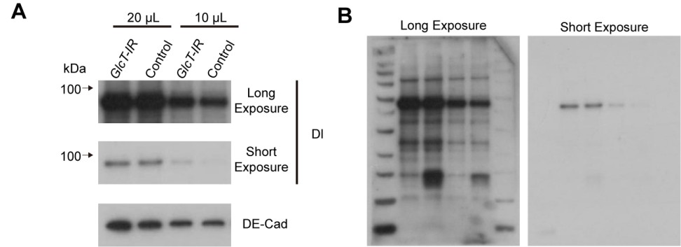
(8) It is unfortunate that GlcT doesn't affect Notch signaling in other organs on the fly. This brings into question the Delta trafficking model and the authors should note this. Also, the clonal marker in Figure 6C is not clear.
In the revised working model, we have explicitly described that the events occur in intestinal stem cells. Regarding Figure 6C, we have delineated the clone with a white dashed line to enhance its clarity and visual comprehension.
(9) The authors state that loss of UGCG in the mouse small intestine results in a reduced ISC count. However, in Supplementary Figure C3, Ki67, a marker of ISC proliferation, is significantly increased in UGCG-CKO mice. This contradiction should be clarified. The authors might repeat this experiment using an alternative ISC marker, such as Lgr5.
Previous studies have indicated that dysregulation of the Notch signaling pathway can result in a reduction in the number of ISCs. While we did not perform a direct quantification of ISC numbers in our experiments, our Olfm4 staining—which serves as a reliable marker for ISCs—demonstrates a clear reduction in the number of positive cells in UGCG-CKO mice.
The increased Ki67 signal we observed reflects enhanced proliferation in the transit-amplifying region, and it does not directly indicate an increase in ISC number. Therefore, in UGCG-CKO mice, we observe a decrease in the number of ISCs, while there is an increase in transit-amplifying (TA) cells (progenitor cells). This increase in TA cells is probably a secondary consequence of the loss of barrier function associated with the UGCG knockout.
On the erosion of middle class America. Poverty line is around 140k if actual costs taken into account. The 1960s benchmark assumed cost of food to be 1/3 of overall costs. Now it's 7% or so, meaning 1/15 of overall costs. This pushes up the poverty line to 5 times the level used, or some 150k USD pa
Example of a proxy being used as 'measurement' and the assumptions in a proxy never re-evaluated.
Author response:
The following is the authors’ response to the previous reviews
Reviewer #3 (Recommendations for the authors):
The authors have done an excellent job of addressing most comments, but my concerns about Figure 5 remain. I appreciate the authors' efforts to address the problem involving Rs being part of the computation on both the x and y axes of Figure 5, but addressing this via simulation addresses statistical significance but overlooks effect size. I think the authors may have misunderstood my original suggestion, so I will attempt to explain it better here. Since "Rs" is an average across all trials, the trials could be subdivided in two halves to compute two separate averages - for example, an average of the even numbered trials and an average of the odd numbered trials. Then you would use the "Rs" from the even numbered trials for one axis and the "Rs" from the odd numbered trials for the other. You would then plot R-Rs_even vs Rf-Rs_odd. This would remove the confound from this figure, and allow the text/interpretation to be largely unchanged (assuming the results continue to look as they do).
We have added a description and the result of the new analysis (line #321 to #332), and a supplementary figure (Suppl. Fig. 1) (line #1464 to #1477).
“We calculated 𝑅<sub>𝑠</sub> in the ordinate and abscissa of Figure 5A-E using responses averaged across different subsets of trials, such that 𝑅<sub>𝑠</sub> was no longer a common term in the ordinate and abscissa. For each neuron, we determined 𝑅<sub>𝑠1</sub> by averaging the firing rates of 𝑅<sub>𝑠</sub> across half of the recorded trials, selected randomly. We also determined 𝑅<sub>𝑠2</sub> by averaging the firing rates of 𝑅<sub>𝑠</sub> across the rest of the trials. We regressed (𝑅 − 𝑅<sub>𝑠1</sub> ) on (𝑅<sub>𝑓</sub> − 𝑅<sub>𝑠2</sub>) , as well as (𝑅<sub>𝑠</sub> - 𝑅<sub>𝑠2</sub>) on (𝑅<sub>𝑓</sub> − 𝑅<sub>𝑠1</sub>), and repeated the procedure 50 times. The averaged slopes obtained with 𝑅<sub>𝑠</sub> from the split trials showed the same pattern as those using 𝑅<sub>𝑠</sub> from all trials (Table 1 and Supplementary Fig. 1), although the coefficient of determination was slightly reduced (Table 1). For ×4 speed separation, the slopes were nearly identical to those shown in Figure 5F1. For ×2 speed separation, the slopes were slightly smaller than those in Figure 5F2, but followed the same pattern (Supplementary Fig. 1). Together, these analysis results confirmed the faster-speed bias at the slow stimulus speeds, and the change of the response weights as stimulus speeds increased.”
An additional remaining item concerns the terminology weighted sum, in the context of the constraint that wf and ws must sum to one. My opinion is that it is non-standard to use weighted sum when the computation is a weighted average, but as long as the authors make their meaning clear, the reader will be able to follow. I suggest adding some phrasing to explain to the reader the shift in interpretation from the more general weighted sum to the more constrained weighted average. Specifically, "weighted sum" first appears on line 268, and then the additional constraint of ws + wf =1 is introduced on line 278. Somewhere around line 278, it would be useful to include a sentence stating that this constraint means the weighted sum is constrained to be a weighted average.
Thanks for the suggestion. We have modified the text as follows. Since we made other modifications in the text, the line numbers are slightly different from the last version.
Line #274 to 275:
“Since it is not possible to solve for both variables, 𝑤<sub>𝑠</sub> and 𝑤<sub>𝑓</sub>, from a single equation (Eq. 5) with three data points, we introduced an additional constraint: 𝑤<sub>𝑠</sub> + 𝑤<sub>𝑓</sub> =1. With this constraint, the weighted sum becomes a weighted average.”
Also on line #309:
“First, at each speed pair and for each of the 100 neurons in the data sample shown in Figure 5, we simulated the response to the bi-speed stimuli (𝑅<sub>𝑒</sub>) as a randomly weighted average of 𝑅<sub>𝑓</sub> and 𝑅<sub>𝑠</sub> of the same neuron.
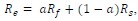
in which 𝑎 was a randomly generated weight (between 0 and 1) for 𝑅<sub>𝑓</sub>, and the weights for 𝑅<sub>𝑓</sub> and 𝑅<sub>𝑠</sub> summed to one.”
Gălûñ′lătĭ
Gălûñ′lătĭ, secondo la mitologia Cherokee, è un mondo creato prima dell'esistenza della Terra.
[https://www.cherokeepins.org/post/cherokee-stories-and-the-birth-of-a-new-world-the-first-fire]
Note: This response was posted by the corresponding author to Review Commons. The content has not been altered except for formatting.
Learn more at Review Commons
Reviewer #1 (Evidence, reproducibility and clarity (Required)): The authors map the ZFP36L1 protein interactome in human T cells using UltraID proximity labeling combined with quantitative mass spectrometry. They optimize labeling conditions in primary T cells, profile resting and activated cells, and include a time course at 2, 5, and 16 hours. They complement the interactome with co-immunoprecipitation in the presence or absence of RNase to assess RNA dependence. They then test selected candidates using CRISPR knockouts in primary T cells, focusing on UPF1 and GIGYF1/2, and report effects on global translation, stress, activation markers, and ZFP36L1 protein levels. The work argues that ZFP36L1 sits at the center of multiple post-transcriptional pathways in T cells (which in itself is not a novel finding) and that UPF1 supports ZFP36L1 expression at the mRNA and protein level. The main model system is primary human T cells, with some data in Jurkat cells.
The core datasets show thousands of identified proteins in total lysates and enriched biotinylated fractions. Known partners from CCR4-NOT, decapping, stress granules, and P-bodies appear, with additional candidates like GIGYF1/2, PATL1, DDX6, and UPF1. Time-resolved labeling suggests shifts in proximity during early activation. Co-IP with and without RNase suggests both RNA-dependent and RNA-independent contacts. CRISPR loss of UPF1 or GIGYF1/2 increases translation at rest and elevates activation markers, and UPF1 loss reduces ZFP36L1 protein and mRNA while MG132 does not rescue protein levels; UPF1 RIP enriches ZFP36L1 mRNA.
Among patterns worth noting are that the activation state drives the principal variance in both proteome and proximity datasets. Deadenylation, decapping, and granule proteins are consistently near ZFP36L1 across conditions, while some contacts dip at 2 hours and recover by 5 to 16 hours. Mitochondrial ribosomal proteins become more proximal later. UPF1 and GIGYF1 show time-linked behavior and RNase sensitivity that fits roles in mRNA surveillance and translational control. These observations support a dynamic hub model, though they remain proximity-based rather than direct binding maps.
We thank the reviewer for their careful reading and thoughtful summary. Please find our point-to point response below.
Major comments
1) The key conclusions are directionally convincing for a broad and dynamic ZFP36L1 neighborhood in human T cells. The data robustly recover established complexes and add plausible candidates. The time-course and RNase experiments strengthen the claim that interactions shift with activation state and RNA context. The functional tests around UPF1 and GIGYF1/2 point to biological relevance. That said, some statements could be qualified. The statement that ZFP36L1 "coordinates" multiple pathways implies mechanism and directionality that proximity data alone cannot prove. I suggest reframing as "positions ZFP36L1 within" or "supports a model where ZFP36L1 sits within" these networks.
We thank this reviewer for considering our data ‘directionally convincing, and robust, adding new plausible candidates as interactors with ZFP36L1’. We agree that the proposed wording is more appropriate and will change it accordingly.
2) UPF1, as an upstream regulator of ZFP36L1 expression, is a promising lead. The reduction of ZFP36L1 protein and mRNA in UPF1 knockout, the non-rescue by MG132, and the UPF1 RIP on ZFP36L1 mRNA together argue that UPF1 influences ZFP36L1 transcript output or processing. This claim would read stronger with one short rescue or perturbation that pins the mechanism. A compact test would be UPF1 re-expression in UPF1-deficient T cells with wild-type and helicase-dead alleles. This is realistic in primary T cells using mRNA electroporation or virus-based systems. Approximate time 2 to 3 weeks, including guide design check and expansion. Reagents and sequencing about 2 to 4k USD depending on donor numbers. This would help separate viability or stress effects from a direct role in ZFP36L1 mRNA handling.
We agree that a rescue experiment with wild-type and helicase-dead UPF1 in UPF1-deficient primary T cells would be interesting. Unfortunately, however, UPF1 knockout T cells are less viable and divide less (Supp Figure 6B), making further manipulations such as re-expression by viral transduction technically impossible. We will clarify this limitation in the Discussion and will more explicitly indicate that UPF1 promotes ZFP36L1 mRNA and protein expression, while acknowledging that the precise mechanistic contribution of UPF1 (e.g. to transcript processing, export, or surveillance) remain to be fully resolved.
3) The inference that ZFP36L1 proximity to decapping and deadenylation complexes reflects pathway engagement is reasonable and, frankly, expected. Still, where the manuscript moves from proximity to function, the narrative works best when supported by orthogonal validation. Two compact additions would raise confidence without opening new lines of work. First, a small set of reciprocal co-IPs for PATL1 or DDX6 at endogenous levels in activated T cells, run with and without RNase, would tie the RNase-class assignments to biochemistry. Second, a short-pulse proximity experiment using a reduced biotin dose and shorter labeling window in activated cells would address whether long incubations drive non-specific labeling. Both are feasible in 2 to 3 weeks with minimal extra cost for antibodies and MS runs if the facility is in-house.
We fully agree with the reviewer that orthogonal biochemical validation is valuable. Therefore, we already combined time-resolved proximity labeling (between 0-2h, 2-5h, and 5-16 hours) with time-resolved ZFP36L1 co-IPs ± RNase, to address the dynamic behavior and potential temporal broadening of the interactome.
As to running reciprocal co-IPs for PATL1 or DDX6: we had in fact already considered to follow up on PATL1. However, we failed to identified specific antibodies, revealing many unspecific bands (see below). As to DDX6, antibodies suitable for IP have been reported, and we can therefore offer such reciprocal IP as requested.
To further address the raised points, we will (i) clarify how we define and interpret RNase-sensitive versus RNase-resistant classes (ii) emphasize that some key factors (including PATL1) are already detected in shorter labeling conditions (2 h) in activated T cells (Fig 4C); and (iii) better highlight that the our data provide strong candidates and pathway hypotheses that warrant further mechanistic experimentation in follow-up studies, when moving from proximity to function.
As to the suggested lowering dose of biotin: As described in Figure S1, this appeared unsuccessful. We owe it to the reported dependence and use of biotin in primary T cells (Ref’s 31-33 of this manuscript). This also included that we could not culture T cells in biotin-free medium prior to labeling, as most protocols would do in cell lines.
The reviewer also suggested shorter labeling times. Please be advised that the labeling times chosen were based on the reported protein induction and activity on target mRNAs: 1) ZFP36L1 expression peaks at 2h of T cell activation (Zandhuis et al. 2025; 0.1002/eji.202451641, Petkau et al. 2024; 10.1002/eji.202350700), 3) shows the strongest effects on T cell function between 4-5h, and displays a late phase of activity at 5-16h (Popovic et al. Cell Reports 2023; 10.1016/j.celrep.2023.112419). We realize that additional explanation is warranted for this rationale, which we will provide.
4) Reproducibility is helped by donor pooling, repeated T-cell screens, Jurkat confirmation, and detailed methods including MaxQuant, LIMMA, and supervised patterning. Deposition of MS data is listed. The authors should consider adding a brief, stand-alone analysis notebook in SI or on GitHub with exact filtering thresholds and "shape" definitions, since the supervised profiles are central to claims. This would let others reproduce figures from raw tables with the same code and workflows.
We thank the reviewer for his or her suggestion and we have done as suggested. We will include the following link in the manuscript: https://github.com/ajhoogendijk/ZFP36L1_UltraID
5) Replication and statistics are mostly adequate for discovery proteomics. The thresholds are clear, and PCA and correlation frameworks are appropriate. For functional readouts in edited T cells, please make the number of donors and independent experiments explicit in figure legends, and indicate whether statistics are paired by donor. Where viability differs (UPF1), note any gating strategies used to avoid bias in puromycin or activation marker measurements. These clarifications are quick to add.
Please be advised that the current figure legends already contain the requested information at the bottom (which test used, donor number etc). To highlight this better, we will indicate this point more explicitly in the methods section.
Minor comments 6) The UltraID optimization in primary T cells is useful, but the long 16-hour labeling and high biotin should be framed as a compromise rather than a standard. A short statement about potential off-target labeling during extended incubations would set expectations and justify the RNase and time-course controls.
Please be advised that 1) high biotin was required because primary T cells depend on biotin and 2) increase biotin absorption a 2-7-fold upon activation (Ref 31-33 from the paper). For better time resolution, we included a labeling of 2h (from 0-2h of activation), 3h (from 2-5h) and 9h (from 5-16h) of T cell activation. Nevertheless, we agree that we cannot exclude the risk of off-target labeling, which in fact is inherent to any labeling and pulldown method. We will include such statement in the discussion.
7) The overlap across T-cell screens and with HEK293T APEX datasets is discussed, but a compact quantitative reconciliation would help. A table that lists shared versus cell-type-specific interactors with brief notes on known expression patterns would make this point concrete.
We thank the reviewer for this suggestion. We agree and we will include such table.
8) Figures are generally clear. Where proximity and total proteome PCA are shown, consider adding sample-wise annotations for donor pools and activation time to help readers link variance to biology. Ensure all volcano plots and heatmaps display the exact cutoffs used in text.
We agree that sample-wise annotations would be a nice addition. However, when testing this for e.g. FIgure 1D&E, such differentiation into individual donors becomes illegible due to the many different variables already present. We therefore decided against it.
9) Prior work on ZFP36 family roles in decay, deadenylation via CCR4-NOT, granules, and translational control is cited within the manuscript. In a few places, recent proximity and interactome papers could be more explicitly integrated when comparing overlap, especially where conclusions differ by cell type. A concise paragraph in Discussion that lays out what is truly new in primary T cells would help clarify the contribution of this work to the field.
We appreciate this suggestion and will revise the Discussion accordingly. As to what is new in primary T cells, we would also like to mention that adding H2O2 (required for APEX labeling) to T cells results in immediate cell death can therefore not be employed on T cells. This technical limitation further underscores the valuable contribution of the UltraID-based approach we present here.
Reviewer #1 (Significance (Required)):
Nature and type of advance. The study is a technical and contextual advance in mapping ZFP36L1 proximity partners directly in human primary T cells during activation. The combination of time-resolved labeling and RNase-class assignments is informative. The CRIS PR perturbations provide an initial functional bridge from proximity to phenotype, especially for UPF1.
Context in the literature. ZFP36 family proteins have long been linked to ARE-mediated decay, CCR4-NOT recruitment, and granule localization. The present work confirms those cores and extends them to include decapping and GIGYF1/2-4EHP scaffolds in primary T cells with temporal resolution. The UPF1 link to ZFP36L1 expression adds a plausible surveillance angle that merits follow-up. The cell-type specificity analysis versus HEK293T underscores that proximity networks vary with context.
Audience. Readers in RNA biology, T-cell biology, and proteomics will find the dataset valuable. Groups studying post-transcriptional regulation in immunity can use the resource to prioritize candidate nodes for mechanistic work.
Expertise and scope. I work on post-transcriptional regulation, RNA-protein complexes, and T-cell effector biology. I am comfortable evaluating the conceptual claims, experimental design, and statistical treatment. I am not a mass spectrometry specialist, so I rely on the presented parameters and deposited data for MS acquisition specifics.
To conclude, the manuscript delivers a substantive proximity map of ZFP36L1 in human T cells, with useful temporal and RNA-class information. The UPF1 observations are promising and would benefit from a compact rescue to secure causality. A few minor additions for biochemical validation and transparency in replication would further strengthen the paper.
We thank the reviewer for this comprehensive and constructive assessment. We agree that our study primarily provides a substantive and well-annotated proximity map of ZFP36L1 in human T cells, including temporal and RNA-class information, and that the UPF1 observations constitute a promising lead that merits more detailed mechanistic analysis in follow-up studies.
Reviewer #2 (Evidence, reproducibility and clarity (Required)): The manuscript by Wolkers and colleagues describes the protein interactome of the RNA-binding protein ZFP36L1 in primary human T-cells. There is inherent value in the use of primary cells of human origin, but there is also value in that the study is quite complete, as it is performed in a variety of conditions: T-cells that have been activated or not, at different time points after activation, and by two methods (co-IP and proximity labeling). One might imagine that this basically covers all what can be detected for this protein in T-cells. The authors report a large amount of new interactors involved at all steps in post-transcriptional regulation. In addition, the authors show that UPF1, a known interactor of ZFP36L1, actually binds to ZFP36L1 mRNA and enhances its levels. In sum, the work provides a valuable resource of ZFP36L1 interactors. Yet, how the data add to the mechanistic understanding of ZFP36L1 functions and/or regulation of ZFP36L1 remains unclear.
We thank the reviewer for this enthusiasm on our experimental setups, considering the use of primary T cells of inherent value and our study with the variety of conditions complete.
Major comments: 1) Fig 2: It is confusing that the Pearson correlation to define ZFP36L1 interactors is changed depending on figure panel. In panels A-C, a correlation {greater than or equal to} 0.6 is used, while panel D uses a correlation > 0.5, which changes the nº of interactors. Then, this is changed again in Fig 3A for some cell types but not for others. Why has this been done? It would be better to stick to the same thresholds throughout the manuscript.
Please be advised that different correlation thresholds arise from the composition of the individual datasets: they in depth, number of controls, and the overall dynamic range. The initial proximity labeling experiment (Figure 2A–C) had a higher depth and a larger number of suitable control samples, which allowed us to apply a stricter cutoff (r ≥ 0.6). The time-course experiment and some of the cross-cell-type comparisons have fewer controls and somewhat lower depth, which then required a more permissive threshold (e.g. r > 0.5) to retain known core interactors.
We fully agree that this rationale needs to be explicit. In the revised manuscript we (i) clearly state for each dataset which correlation cutoff is used (ii) emphasize that these thresholds are somewhat arbitrary and should not be directly compared across experiments, and (iii) highlight that our key biological conclusions do not depend on the exact boundary chosen but rather on the consistent enrichment of core complexes and pathways across .
2) Fig 3A: It would be nice to have the information of this Figure panel as a Table (protein name, molecular process(es), known or novel, previously detected in which cells) in addition to the figure.
We agree that this would increase the value of our work as a resource to the community, and we will include such table and merge it with the table Reviewer 1 asked about.
3) Fig 6: To what extent are the effects of UPF1 and GIGFYF1 knock-out on translation and T-cell hyper-activation mediated by ZFP36L1? If deletion of ZFP36L1 itself has no effect on these processes, it seems unlikely that it is involved. In this respect, I am not sure that Fig 6 contributes to the understanding of ZFP36L.
We appreciate this conceptual question. In our dataset, ZFP36L1 knockout affects T-cell activation markers, but does not recapitulate the increased global translation observed upon UPF1 or GIGYF1/2 deletion. We will discuss this finding more explicitly in the Results and Discussion. We discuss the possibility that other ZFP36 family members (e.g. ZFP36/TTP, ZFP36L2) may partially compensate for the absence of ZFP36L1 in some readouts1. Moreover, we will emphasize that at this point it is not clear whether ZFP36L1’s contribution to UPF1 and GIGYF1 protein levels is direct or indirect.
We nonetheless consider Fig. 6 an important component of the story, as it demonstrates that proximity partners emerging from the interactome (UPF1, GIGYF1/2) have measurable functional consequences on T cell activation and translational control, thereby illustrating how the resource can guide mechanistic hypotheses. We will now more carefully phrase this as “first indications of mechanism” and avoid implying that these phenotypes are mediated exclusively via ZFP36L1.
4) Fig 7E: Differences in ZFP36L1 mRNA expression are claimed as a consequence of UPF1 deletion, and indeed there is a clear tendency to reduction of ZFP36L1 mRNA levels upon UPF1 KO. Yet the difference is statistically non-significant. Please, repeat this experiment to increase statistical significance. In addition, a clear discussion on how UPF1 -generally associated to mRNA degradation- contributes to increase ZFP36L1 mRNA levels would be appreciated.
We would like to refrain from including repeats for increasing statistical power. We find similar trends with n=3 at 0h as with n=7 at 3h of activation (Fig. 7E). We rather would like to stress that despite the width overall expression levels which most probably stems from using primary human material, the overall levels of ZFP36L1 mRNA are lower in UPF1 KO T cells. We will include a point on how UPF1 possibly may contribute to the decreased ZFP36L1 mRNA levels, as suggested.
5) Fig 6A: The decrease in global translation by GIGFYF1 knock-out upon activation claimed by the authors is not clear in Fig 6A and is non-significant upon quantification. Please, modify narrative accordingly.
Indeed, this was not phrased well. We will correct our description to match the statistical analysis.
6) Page 6: The authors state 'This included the PAN2/3 complex proteins which trim poly(A) tails prior to mRNA degradation through the CCR4/NOT complex'. To the best of my knowledge, the CCR4/NOT complex does not degrade the body of the mRNA. Both PAN2/3 and CCR4/NOT are deadenylases that function independently.
We thank the reviewer for highlighting this inaccuracy. PAN2/3 and CCR4–NOT are indeed both deadenylase complexes that function independently rather than one acting strictly upstream of the other in degrading the mRNA body. We will correct this statement to that PAN2/3 and CCR4–NOT cooperate in poly(A) tail shortening and do not themselves degrade the mRNA body, which is instead handled by the downstream decay machinery.
7) Please, label all Table sheets. Right now one has to guess what is being shown in most of them. Furthermore, it would be convenient to join all Tables related to the same Figure in one unique Excel with several sheets, rather than having many Tables with only one sheet each.
We appreciate this suggestion. In the revised supplementary files all table sheets will be clearly labeled to indicate the corresponding figure and dataset, and combined into a single excel file when multiple tables relate to the same figure. We have already done so.
Minor comments: 8) Fig 1E: Shouldn't there be a better separation by biotinylation in the UltraID IP principal component analysis? In theory, only biotinylated proteins should be immunoprecipitated.
In theory this should indeed be the case. However, in practice, pull down experiments always suffer from background stickiness of proteins to tubes, beads etc. Combined, these known background issues highlight the critical addition of control samples, allowing for unequivocal call of proteins that are above background.
In addition, as we indicated in the manuscript, primary T cells depend on Biotin. This prohibited us to use biotin-free medium, even for a short culture period (it resulted in cell death). Such biotin-free culture steps are included in proximity labeling assays performed in cell lines. Owing to the continuous addition of biotin, some of the ‘background’ biotinylation signal may even be ‘real’. Nevertheless, the higher levels of biotin we added during the labeling results in increased signals, and statistical analysis with these controls identifies which of the proteins are above background, irrespective from the source. We will include a short note on this in the manuscript
9) Fig 3B-E: Is the labeling not swapped, top (always +) is Biotin and bottom (- or +) is aCD3/aCD28?
We thank the reviewer for catching this mistake- we have corrected it
10) Fig 7A data is from another paper, so I suggest to move this panel to Supplementary materials.
We respectfully disagree. Please be advised that we reanalysed data from published datasets, that resulted in this figure. Re-analysis is a widely accepted method and certainly used for main figure panels. Our re-analysis from Bestenhorn et al 2025; (10.1016/j.molcel.2025.01.001) confirms that ZFP36L1 interacts with UPF1 and GIGYF1/2 in the RAW 264.7 macrophage cell line, which we consider an important consolidation of our findings. To highlight that this table is a re-analysis of published data, we will include this information (including the reference) below the data. As ‘extracted from Bestenhorn et al'
11) Fig S1A: Why is there so much labeling in the UltraID only lane without biotin?
This is a phenomenon also reported by others (Kubitz et al. 2022; 10.1038/s42003-022-03604-5: Figure 5A). UltraID alone is a small protein of (19.7KD), comparable to TurboID or others (Kubitz et al. 2022; 10.1038/s42003-022-03604-5). If not tethered to a specific compartment, these proximity labeling moieties can diffuse through the cytoplasm, biotinylating any protein they ‘bump’ into. Please be advised that we included this control to show this effect, to substantiate why we use GFP-UltraID- as control, to limit such background effects. To highlight this point better, we will better articulate this reasoning in the results section.
12) Fig S1E: Please, explain better. What is WT?
We thank the reviewer for catching this inconsistency. We will explicitly define “WT” as wild-type primary T cells (non-edited, non-transduced) and clarify how this relates to the other conditions.
13) Fig S4B: Please, explain the labels on top of the shapes.
We will update the figure, explaining how the labels above each shape are chosen (e.g. indicating specific clusters, functional categories, or experimental conditions, as appropriate). This should make the reading more intuitive.
14) Page 3: A time-course of incubation with biotin is lacking in Fig S1B, and thereby it is confusing that the authors direct readers to this figure when an increased to 16h incubation is claimed to be better.
Please be advised that short labeling times yielded disappointing results in primary human T cells. Therefore all first analyses were performed with 16h biotinylation, as depicted in Figure S1B). Only after achieving good results (presented in Figure 1B), we performed time course experiments (presented in __Figure 4, __lowering incubation times to 2h, 3h and 9h). We realize that this is confusing and we will rephrase this point in page 3.
Reviewer #2 (Significance (Required)): Strengths: A thorough repository of ZFP36L1 interactors in primary human T-cells. A valuable resource for the community. Weaknesses: There is little mechanistic insight on ZFP36L1 function or regulation.
We would like to highlight that the purpose of our study was to provide a comprehensive interactome of ZFP36L1, and to study the dynamics of these interactions. In addition to known interactors, we identified novel putative interactors of ZFP36L1. We have indeed not followed up on all interactions, which we consider beyond the scope of this manuscript. Rather, we consider our study as a toolbox for the community, that helps in their studies.
Nevertheless, in Fig 6-7, we show first indications of mechanistic insights on ZFP36L1 interactors, exemplifying how the findings of this resource paper can be used by the community.
Reviewer #3 (Evidence, reproducibility and clarity (Required)):
The authors have analyzed the interactome of ZFP36L1 in primary human T cells using a biotin-based proximity labeling method. In addition to proteins that are known to interact with ZFP36L1, the authors defined a multitude of novel interactions involved in mRNA decapping, mRNA degradation pathways, translation repressors, stress granule/p-body formation, and other regulatory pathways. Time-lapse proximity labeling revealed that the ZFP36L1 interactome undergoes remodeling during T cell activation. Co-IP for ZFP36L1 executed in the presence/absence of RNA further revealed the interactome and possible regulators of ZFP36L1, including the helicase UPF1. In addition to interacting with ZFP36L1, UPF1 promotes the ZFP36L1 protein expression, seemingly by binding to the ZFP36L1 mRNA transcript, and in some way stabilizing it. This comprehensive interactome map highlights the widespread interactions of ZFP36L1 with proteins of many types, and its potential roles in diverse T cell processes. Although somewhat descriptive, rather than hypothesis-testing, this work represents an important contribution to understanding the potential roles of the ZFP36 family proteins, and sets up many future experiments which could test molecular details.
We thank the reviewer for these thoughtful points, and for recognizing our paper as an important contribution for the field as resource, that should support future experiments.
Major points: 1) Can the authors discuss the specificity of the antibody for ZFP36L1 used in the Co-IP experiments? The antibody listed in Appendix A is abcam catalog number ab42473, although the catalog number for this antibody (unlike the others major ones used) is not listed in the Methods section - please add this to the Methods to make it easier for readers to find this detail. Could this antibody also be immunoprecipitating ZFP36 or ZFP36L2? Other antibodies have had cross-reactivity for the different family members. It is also notable that this antibody has been discontinued by the manufacturer (https://www.abcam.com/en-us/products/unavailable/zfp36l1-antibody-ab42473). Have the authors tried the current abcam anti-ZFP36L1 antibody being sold, catalog number ab230507?
We appreciate the opportunity to clarify this important technical point. We have now added the catalog number (ab42473, Abcam) of the anti-ZFP36L1 antibody used for co-IP to the Methods section, in addition to Appendix A, to facilitate reproducibility. The antibody ab42473 has indeed been discontinued by the manufacturer. We have contacted the manufacturer on multiple occasions with no luck.
We have evaluated multiple alternative anti-ZFP36L1 antibodies, including the currently available Abcam antibody ab230507. In our hands, these alternatives showed weaker or less specific detection of ZFP36L1 compared to the original ZFP36L1 antibody. Only antibody 1A3 recognized ZFP36L1. We therefore used this antibody for the Co-IP. Importantly, even though the signal is lower than the original antibody we used, the migration patterns observed with ab42473 in our co-IP experiments match the expected molecular weight of ZFP36L1 and do not suggest substantial cross-reactivity with ZFP36 or ZFP36L2, which display distinct sizes (we will add the sizes to the WB in figures). We discuss this point briefly in the revised Methods/Results.
2) On this point, the authors report interactions between ZFP36L1 and its related proteins ZFP36 and ZFP36L2 in the Co-IP experiment (Supp 5C). Did these proteins interact in the proximity labeling? Ideally this could be discussed in the Discussion section.
ZFP36 and ZFP36L2 were indeed detected as co-precipitating with ZFP36L1 in the co-IP experiments but were not found as high-confidence interactors in the UltraID proximity labeling datasets. Also in the APEX proximity labeling of Bestehorn et al. In RAW macrophage cells, they did not find ZFP36 or ZFP36L1 to interact with ZFP36L1. * *We now explicitly mention this in the Results and discuss it in the Discussion.
3) Can the authors discuss more fully the limited overlap in identified interactors across the two proximity labeling screens performed in primary T cells (Fig 2C)? Likewise, can the authors comment on the very limited overlap between the screens in T cells and the published ZFP36L1-APEX proximity labelling experiment performed in the HEK293T cell line by Bestehorn et al. (ref 42)? Only 6.8% of proteins found in either T cell screen were found as interactors in this cell line. The authors comment that this may be because "...either expression of certain proteins is cell-type specific, or [because] ZFP36L1 has cell-type specific protein interactions, in addition to its core interactome". While I agree that cell-type specific interactions may be at play, I would think most of the interactors found in the T cell screens are widely expressed proteins necessary for central cell functions.
First, the apparent overlap percentage depends on depth and filtering. As noted above and now detailed in a new Supplementary table, a core set of decapping, deadenylation, and granule-associated factors is consistently recovered across our T-cell screens and the HEK293T APEX dataset. However, beyond this core protein, overlap is reduced, reflecting several factors: (i) differences in expression levels of many interactors between HEK293T cells and primary T cells; (ii) the activation-dependent nature of ZFP36L1 function in T cells, which cannot be fully mimicked in HEK293T; (iii) different proximity labeling enzymes and fusion constructs (APEX vs UltraID, different tags, expression levels); and (iv) distinct experimental designs and control strategies, which influence statistical filtering and the effective “depth” of each interactome.
In the revised Discussion and in the new comparative table, we now emphasize that while many of the ZFP36L1 proximity partners identified in T cells are indeed widely expressed, their effective labeling and enrichment are strongly context dependent. We therefore interpret the relatively limited overlap as highlighting both a robust core interactome and substantial context-specific remodeling, rather than as evidence of artifacts in one or the other dataset.
Minor comments: 4) In Figure 3D, the legend states that black circles indicate significantly enriched proteins in biotin samples, while grey circles indicate non-significant enrichment. However, some genes, including DCP1A, DDX6, YBX1, have black circles in the -biotin group and grey in the +biotin group, which creates confusion in interpretation.
We thank the reviewer for this comment. We have accidentally switched the labeling of biotin and activation as pointed out by reviewer 2. Once this is fixed, this comment will also be fixed.
5) Did the authors find any interactors whose expression is known to be specific to CD4 or CD8 T cells?
In our current dataset we did not identify interactors whose presence was clearly restricted to CD4 or CD8 T-cells. We agree that differential ZFP36L1 interactomes in defined T-cell subsets represent an interesting avenue for future targeted studies and will outline this is the discussion.
Reviewer #3 (Significance (Required)):
The authors present the first comprehensive analysis of the ZFP36L1 interactome in primary T cells. The use of biotin-based proximity labeling enables detection of physiologically relevant interactions in live cells. This approach revealed many novel interactors.
Strengths include the overall richness of the dataset, and the hypothesis-provoking experiments that could follow in the future. Limitations include somewhat limited overlap with a published proximity labeling dataset from performed in a different cell line, suggesting that there may be artifacts in one or both datasets.
The audience for this article would include those interested broadly in RNA binding proteins and those interested in post-transcriptional and translational regulation.
I have immunology expertise on T cell activation and differentiation and expertise on transcriptional and post-transcriptional regulation of gene expression in T cells.
Note: This preprint has been reviewed by subject experts for Review Commons. Content has not been altered except for formatting.
Learn more at Review Commons
The manuscript by Wolkers and colleagues describes the protein interactome of the RNA-binding protein ZFP36L1 in primary human T-cells. There is inherent value in the use of primary cells of human origin, but there is also value in that the study is quite complete, as it is performed in a variety of conditions: T-cells that have been activated or not, at different time points after activation, and by two methods (co-IP and proximity labeling). One might imagine that this basically covers all what can be detected for this protein in T-cells. The authors report a large amount of new interactors involved at all steps in post-transcriptional regulation. In addition, the authors show that UPF1, a known interactor of ZFP36L1, actually binds to ZFP36L1 mRNA and enhances its levels. In sum, the work provides a valuable resource of ZFP36L1 interactors. Yet, how the data add to the mechanistic understanding of ZFP36L1 functions and/or regulation of ZFP36L1 remains unclear.
Major comments:
1) Fig 2: It is confusing that the Pearson correlation to define ZFP36L1 interactors is changed depending on figure panel. In panels A-C, a correlation {greater than or equal to} 0.6 is used, while panel D uses a correlation > 0.5, which changes the nº of interactors. Then, this is changed again in Fig 3A for some cell types but not for others. Why has this been done? It would be better to stick to the same thresholds throughout the manuscript.
2) Fig 3A: It would be nice to have the information of this Figure panel as a Table (protein name, molecular process(es), known or novel, previously detected in which cells) in addition to the figure.
3) Fig 6: To what extent are the effects of UPF1 and GIGFYF1 knock-out on translation and T-cell hyper-activation mediated by ZFP36L1? If deletion of ZFP36L1 itself has no effect on these processes, it seems unlikely that it is involved. In this respect, I am not sure that Fig 6 contributes to the understanding of ZFP36L.
4) Fig 7E: Differences in ZFP36L1 mRNA expression are claimed as a consequence of UPF1 deletion, and indeed there is a clear tendency to reduction of ZFP36L1 mRNA levels upon UPF1 KO. Yet the difference is statistically non-significant. Please, repeat this experiment to increase statistical significance. In addition, a clear discussion on how UPF1 -generally associated to mRNA degradation- contributes to increase ZFP36L1 mRNA levels would be appreciated.
5) Fig 6A: The decrease in global translation by GIGFYF1 knock-out upon activation claimed by the authors is not clear in Fig 6A and is non-significant upon quantification. Please, modify narrative accordingly.
6) Page 6: The authors state 'This included the PAN2/3 complex proteins which trim poly(A) tails prior to mRNA degradation through the CCR4/NOT complex'. To the best of my knowledge, the CCR4/NOT complex does not degrade the body of the mRNA. Both PAN2/3 and CCR4/NOT are deadenylases that function independently.
7) Please, label all Table sheets. Right now one has to guess what is being shown in most of them. Furthermore, it would be convenient to join all Tables related to the same Figure in one unique Excel with several sheets, rather than having many Tables with only one sheet each.
Minor comments:
8) Fig 1E: Shouldn't there be a better separation by biotinylation in the UltraID IP principal component analysis? In theory, only biotinylated proteins should be immunoprecipitated.
9) Fig 3B-E: Is the labeling not swapped, top (always +) is Biotin and bottom (- or +) is aCD3/aCD28?
10) Fig 7A data is from another paper, so I suggest to move this panel to Supplementary materials.
11) Fig S1A: Why is there so much labeling in the UltraID only lane without biotin?
12) Fig S1E: Please, explain better. What is WT?
13) Fig S4B: Please, explain the labels on top of the shapes.
14) Page 3: A time-course of incubation with biotin is lacking in Fig S1B, and thereby it is confusing that the authors direct readers to this figure when an increased to 16h incubation is claimed to be better.
Strengths: A thorough repository of ZFP36L1 interactors in primary human T-cells. A valuable resource for the community.
Weaknesses: There is little mechanistic insight on ZFP36L1 function or regulation.
Document d'Information : Le Traitement Médiatique des Violences Faites aux Femmes
Ce document d'information synthétise les discussions d'une table ronde sur le traitement médiatique des violences faites aux femmes, réunissant une journaliste d'investigation, une vulgarisatrice et une militante féministe.
Il ressort que si la médiatisation de ce sujet sociétal est croissante, elle est entachée de biais significatifs et de pratiques problématiques. Les points essentiels sont les suivants :
• Le Rôle Ambivalent des Médias : Les médias jouent un rôle crucial en rendant publiques des violences souvent cantonnées à la sphère privée, ce qui permet de faire évoluer les mentalités et de reconnaître le caractère systémique du problème.
Chaque avancée sociétale sur le sujet est liée à la médiatisation d'une affaire emblématique (Mazneff, Depardieu, etc.).
• Critiques Principales du Traitement Médiatique : La couverture médiatique est critiquée pour sa tendance à racialiser les agresseurs, servant un agenda politique raciste en surreprésentant les agresseurs étrangers ou racisés contre des victimes blanches.
On observe également une différence de traitement majeure entre la presse nationale, qui aborde parfois le sujet sous un angle systémique, et la presse locale (PQR), qui le confine souvent au sensationnalisme du "fait divers".
• Éthique Journalistique et Protection des Victimes : Le traitement rigoureux d'une affaire de violence sexiste et sexuelle (VSS) repose sur des principes déontologiques stricts.
La priorité est de croire et de protéger la victime, notamment par l'anonymat, et de respecter son choix de parler ou non.
L'enquête doit être irréprochable pour éviter les risques de diffamation et garantir la crédibilité du récit, ce qui inclut la vérification des faits et la procédure du "contradictoire" (contacter l'agresseur présumé).
• Les Angles Morts de la Médiatisation : De nombreuses formes de violences demeurent largement invisibles.
C'est le cas des violences psychologiques (contrôle, harcèlement numérique via traceurs) et surtout des violences visant les populations les plus marginalisées : les enfants, les travailleuses du sexe et les femmes trans, dont les agressions sont souvent ignorées, voire justifiées par un traitement médiatique transphobe et déshumanisant.
--------------------------------------------------------------------------------
La discussion établit un cadre conceptuel pour analyser le traitement médiatique des violences faites aux femmes, un sujet de plus en plus présent dans le débat public, souvent à travers le prisme d'affaires très médiatisées impliquant des personnalités publiques (PPDA, Gérard Depardieu, Léo Grasset).
Pour analyser les violences, les intervenantes adoptent une approche matérialiste et sociologique.
• Femme : Dans ce contexte, une "femme" n'est pas définie par sa biologie ou son identité de genre, mais comme une personne subissant des conditions sociales spécifiques, notamment le sexisme, les violences et l'exploitation par le système patriarcal.
• Patriarcat : Il est défini comme un système social qui hiérarchise les groupes sociaux "hommes" et "femmes".
Ce système organise l'exploitation (notamment économique via le travail domestique) et l'oppression des femmes, et sanctionne toute personne déviant des normes qu'il impose (ex: hétéronormativité, sanctionnée par l'homophobie).
Les VSS englobent une large gamme de violences, souvent sous-représentées dans leur diversité.
• Violences les plus médiatisées : Le viol et les agressions sexuelles sont les plus visibles médiatiquement, car perçus comme les plus graves.
Les violences conjugales physiques sont également mentionnées, mais les violences psychologiques restent largement ignorées.
• Statistiques et Binarité : Les statistiques disponibles sur les VSS sont majoritairement binaires (hommes/femmes), ce qui invisibilise les victimes non-binaires.
Pauline Bouty souligne que si la plupart des victimes sont des femmes et la plupart des auteurs des hommes, il est crucial de rappeler que des personnes de tous genres peuvent être victimes.
Il est rappelé que près de 90 % des victimes connaissent leur agresseur, qui est souvent un membre de la famille ou le conjoint, contredisant le mythe de l'agresseur inconnu dans une ruelle sombre.
Le traitement médiatique des VSS est considéré comme un enjeu public majeur et non une affaire privée.
• Le "5ème Pouvoir" : Jade Bourgerie, journaliste, qualifie les médias de "5ème pouvoir" dont le rôle est de refléter les maux de la société.
Traiter une affaire de VSS relève de l'intérêt public, car ces violences sont le symptôme d'une "société malade".
• Visibilité et Existence : Selon Pauline Bouty, "ce qu'on ne voit pas n'existe pas".
La médiatisation permet au public de prendre conscience de l'existence et de l'ampleur de ces violences.
Chaque progression dans la compréhension de ce phénomène est directement liée à la couverture médiatique d'une affaire symbolique.
• Déconstruire les Stéréotypes : La médiatisation aide à humaniser les victimes et les agresseurs, brisant l'image du "monstre".
Elle montre que l'agresseur peut être "votre voisin, votre frère, votre oncle", une personne perçue comme sympathique en société.
La journaliste Jade Bourgerie détaille les règles déontologiques qu'elle s'impose pour traiter ces sujets sensibles, en l'absence de règles formelles universelles dans la profession.
1. Respecter et Croire la Victime : Le point de départ est de croire la parole de la victime et de respecter ses volontés.
2. Rigueur de l'Enquête : L'article doit être "parfait" et "solide".
Cela implique de vérifier méticuleusement chaque élément fourni par la victime pour construire un dossier inattaquable et se prémunir contre les accusations de diffamation.
Exemple donné : retrouver une gynécologue consultée par une victime dans les années 90 pour corroborer une partie de son récit.
3. Le Contradictoire : Une étape essentielle consiste à contacter la personne mise en cause (l'agresseur présumé) pour lui exposer les faits recueillis et lui donner la possibilité de se défendre.
L'anonymat est un outil de protection essentiel pour les victimes, en particulier dans les milieux professionnels restreints (ex: musique classique) où tout le monde se connaît. Il permet à la victime d'éviter :
• D'être durablement étiquetée comme "victime de viol".
• De subir des représailles professionnelles ou sociales dans une société encore peu avancée sur ces questions.
Plusieurs problèmes récurrents dans la couverture des VSS sont identifiés par les intervenantes.
Lou Girard dénonce un biais racial majeur : les médias, en particulier ceux détenus par des groupes de droite et d'extrême-droite (citant les "empires Bolloré et Drahi"), tendent à surreprésenter les affaires où des femmes blanches sont agressées par des hommes racisés ou migrants.
Ce traitement sert un "narratif raciste" qui présente "la femme blanche, pure, la Française" comme étant attaquée par "le migrant, l'étranger".
Cela occulte la réalité statistique : la grande majorité des violences sont intra-communautaires et intrafamiliales.
Un clivage important existe entre les types de médias.
Critère
Presse Nationale (ex: Le Monde, Libération)
Presse Quotidienne Régionale (PQR) (ex: La Dépêche)
Traitement
Tendance à traiter les affaires sous un angle plus systémique, souvent liées à des personnalités connues ou à des faits de grande ampleur.
Traitement majoritairement sous le prisme du fait divers et du sensationnalisme.
Biais Racial
Le narratif racialisant est "assez absent" des grands médias nationaux.
Le schéma "femme blanche victime d'un agresseur racisé" est beaucoup plus fréquent.
Causes
Journalistes plus jeunes, formés aux enjeux actuels des VSS dans les écoles de journalisme.
Journalistes souvent en poste depuis des décennies, moins formés à ces problématiques spécifiques.
Le langage utilisé a évolué, mais des termes problématiques persistent.
• Progrès : Le terme "féminicide" a émergé et s'est démocratisé après le mouvement #MeToo. Son usage est politique : il souligne que la victime a été tuée parce qu'elle est une femme, et non dans le cadre d'un simple homicide.
• Persistance : Des termes euphémisants ou inappropriés comme "crime passionnel" ou la description de viols comme des "relations sexuelles imposées" sont encore utilisés, minimisant la notion de violence et de domination.
Certaines violences sont systématiquement absentes de la couverture médiatique.
• Violences Psychologiques : Le contrôle insidieux, qui ne "laisse pas de bleu", est très peu représenté. Pauline Bouty cite le documentaire Traquée de Marine Périn sur les hommes installant des traceurs sur les téléphones de leurs compagnes.
Ce contrôle peut aussi être financier ou social.
• Violences contre les enfants : Les enfants sont particulièrement vulnérables car dépendants des adultes qui sont souvent leurs agresseurs.
• Violences contre les femmes trans : Lou Girard souligne leur vulnérabilité extrême. "En tant que femme on a peur d'être violé, en tant que femme trans on a peur d'être violé puis tué."
Le traitement médiatique, quand il existe, est souvent abominable, utilisant des termes transphobes ("homme travesti") et présentant l'agression comme un fait divers "presque marrant".
Les victimes sont mégenrées, même après leur mort.
• Violences contre les travailleuses du sexe : Leurs agressions sont souvent invisibilisées ou justifiées par leur profession, niant la notion de consentement.
Pour qu'une affaire soit traitée médiatiquement de manière solide, plusieurs critères sont souvent nécessaires du point de vue journalistique :
• Avoir plusieurs victimes : Cela permet d'éviter la situation de "parole contre parole".
• Au moins une victime acceptant de parler à visage découvert : Cela renforce la crédibilité du récit.
• Des faits documentables avec des preuves : Une affaire reposant uniquement sur un témoignage sans plainte ni preuve est quasiment impossible à traiter pour un journaliste.
• Le consentement de la victime : Le respect de la parole de la victime est primordial. De nombreuses affaires ne sortent pas car les victimes ne souhaitent pas parler, un choix qui doit être absolument respecté.
Le Manque de Couverture sur les Conséquences pour les Victimes
Les médias se concentrent sur les faits et les agresseurs, mais très rarement sur l'impact à long terme des violences sur la vie des victimes (psychologique, social, professionnel).
• Analyse Politique : Lou Girard analyse ce manque comme un choix politique.
S'intéresser à la "carrière brisée" de l'agresseur est commun, mais parler des "conséquences terribles du viol" sur la vie des femmes serait un acte "hautement féministe" que beaucoup de médias évitent.
• Le Rôle des Livres : Pauline Bouty nuance en affirmant que ce n'est peut-être pas le rôle des journalistes de parler à la place des victimes de leur ressenti.
Elle défend l'importance des espaces où les victimes peuvent s'exprimer avec leur propre voix, comme les livres (citant Florence Porcel) ou les films (Les Chatouilles).
L'usage de termes précis est un enjeu politique.
• Pédocriminalité vs. Pédophilie : Il est crucial de différencier la pédophilie (une paraphilie, un attrait) de la pédocriminalité (le passage à l'acte).
La plupart des personnes ayant des attirances pédophiles ne passent pas à l'acte et se font suivre. Un pédocriminel cherche avant tout à exercer une emprise et n'est pas nécessairement "pédophile".
• La Voix Active : Il est recommandé d'utiliser la voix active pour nommer l'agresseur et sa responsabilité : "un homme a violé une femme" plutôt que "une femme s'est fait violer".
Présenter les faits est un choix politique : soit on le fait avec des euphémismes, soit on nomme la violence telle qu'elle est.
Author response:
The following is the authors’ response to the original reviews.
Reviewer #1 (Public review):
The authors focus on the molecular mechanisms by which EMT cells confer resistance to cancer cells. The authors use a wide range of methods to reveal that overexpression of Snail in EMT cells induces cholesterol/sphingomyelin imbalance via transcriptional repression of biosynthetic enzymes involved in sphingomyelin synthesis. The study also revealed that ABCA1 is important for cholesterol efflux and thus for counterbalancing the excess of intracellular free cholesterol in these snail-EMT cells. Inhibition of ACAT, an enzyme catalyzing cholesterol esterification, also seems essential to inhibit the growth of snail-expressing cancer cells.
However, It seems important to analyze the localization of ABCA1, as it is possible that in the event of cholesterol/sphingomyelin imbalance, for example, the intracellular trafficking of the pump may be altered.
The authors should also analyze ACAT levels and/or activity in snail-EMT cells that should be increased. Overall, the provided data are important to better understand cancer biology.
We thank the reviewer for recognizing the significance of our study. Consistent with the hypothesis that ABCA1 contributes to chemoresistance in hybrid E/M cells, we agree that demonstrating the localization of ABCA1 at the plasma membrane is important, and we have included additional experiments to address this point.
We also examined the expression of the major ACAT isoform in the kidney, SOAT1, across RCC cell lines. However, its expression did not correlate with that of Snail (Figure 4B), suggesting that SOAT1 is constitutively expressed at a certain level regardless of Snail expression. The details of these additional experiments are provided in the point-by-point responses below.
Reviewer #2 (Public review):
Summary:
In this study, the authors discovered that the chemoresistance in RCC cell lines correlates with the expression levels of the drug transporter ABCA1 and the EMT-related transcription factor Snail. They demonstrate that Snail induces ABCA1 expression and chemoresistance, and that ABCA1 inhibitors can counteract this resistance. The study also suggests that Snail disrupts the cholesterol-sphingomyelin (Chol/SM) balance by repressing the expression of enzymes involved in very long-chain fatty acid-sphingomyelin synthesis, leading to excess free cholesterol. This imbalance activates the cholesterol-LXR pathway, inducing ABCA1 expression. Moreover, inhibiting cholesterol esterification suppresses Snail-positive cancer cell growth, providing potential lipid-targeting strategies for invasive cancer therapy.
Strengths:
This research presents a novel mechanism by which the EMT-related transcription factor Snail confers drug resistance by altering the Chol/SM balance, introducing a previously unrecognized role of lipid metabolism in the chemoresistance of cancer cells. The focus on lipid balance, rather than individual lipid levels, is a particularly insightful approach. The potential for targeting cholesterol detoxification pathways in Snail-positive cancer cells is also a significant therapeutic implication.
Weaknesses:
The study's claim that Snail-induced ABCA1 is crucial for chemoresistance relies only on pharmacological inhibition of ABCA1, lacking additional validation. The causal relationship between the disrupted Chol/SM balance and ABCA1 expression or chemoresistance is not directly supported by data. Some data lack quantitative analysis.
We thank the reviewer for his/her insightful and constructive comments. In response, we have performed additional experiments using complementary approaches to further substantiate the contribution of Snail-induced ABCA1 expression to chemoresistance. Furthermore, to clarify the causal relationship between reduced sphingomyelin biosynthesis and ABCA1 expression, we conducted new experiments showing that supplementation with sphingolipids attenuates ABCA1 upregulation (Figure 3H). The details of these additional experiments are described in the point-by-point responses below.
Reviewer #1 (Recommendations for the authors):
In this paper, the authors reveal that snail expression in EMT-cells leads to an imbalance between cholesterol and sphingomyelin via a transcriptional repression of enzymes involved in the biosynthesis of sphingomyelin.
This paper is interesting and highlights how the imbalance of lipids would impact chemotherapy resistance. However, I have a few comments.
In Figure 2 in Eph4 cells, while filipin staining appears exclusively at the plasma membrane in the case of EpH4-snail cells filipin staining is also intracellular. It seems plausible that all filipin-positive intracellular staining is not exclusively in LDs, authors should therefore try to colocalize filipin with other intracellular markers. To this aim, authors might want to use topfluocholesterol-probe for instance.
We examined the distribution of TopFluor-cholesterol in hybrid E/M cells (Figure 2H) and found that TopFluor-cholesterol colocalizes with lipid droplets. In addition, we analyzed the colocalization between intracellular filipin signals and organelle-specific proteins, ADRP (lipid droplets) and LAMP1 (lysosomes) (Figure 2I). Since filipin binds exclusively to unesterified cholesterol, filipin signals did not colocalize with ADRP. Instead, we observed colocalization of filipin with LAMP1, suggesting that cholesterol accumulates in hybrid E/M cells in both esterified and unesterified forms.
In Figure 3, the authors reveal that the exogenous expression of the snail alters the ratio of cholesterol to sphingomyelin. The authors should reveal where is found the intracellular cholesterol and intracellular sphingomyelin within these cells Eph4-snail.
To investigate the lipid composition of the plasma membrane, we utilized lipid-binding protein probes, D4 (for cholesterol) and lysenin (for sphingomyelin) (Figures 2L and 2M). We found that the plasma membrane cholesterol content was not affected by EMT, whereas sphingomyelin levels were markedly decreased. In addition, intracellular cholesterol was visualized (Comment 1-1; Figures 2E–2K). On the other hand, because visualization of intracellular sphingomyelin is technically challenging, we were unable to include this analysis in the present study. We consider this an important direction for future investigation.
Regarding the model described in panel K of Figure 3. I would expect that the changes in lipid-membrane organization depicted in panel K should affect the pattern of GM1 toxin for instance or the motility of raft-associated proteins for instance. The authors could perform these experiments in order to sustain the change of lipid plasma membrane organization.
We attempted staining with FITC–cholera toxin to visualize GM1, but both EpH4 and EpH4–Snail cells exhibited very low levels of GM1, resulting in minimal or no detectable staining (data not shown). Instead, to assess the impact of decreased sphingomyelin on the overall biophysical properties of the plasma membrane, we used a plasma membrane–specific lipid-order probe, FπCM–SO₃ (Figures 2N–2P and Figure 2—figure supplement 3). We found that the plasma membrane of EpH4–Snail cells was more disordered (fluidized), suggesting that the overall properties of the plasma membrane are altered by ectopic expression of Snail.
Another issue is the intracellular localization of ABCA1 in Eph4-Snail cells. Knowing that a change in the cholesterol/sphingomyelin ratio can also modify intracellular protein trafficking, it seems important to analyze the intracellular localization of ABCA1 in EPh4-Snail cells.
We performed immunofluorescence microscopy for ABCA1 and found that ABCA1 was mainly localized at the plasma membrane in EpH4–Snail cells (Figure 1M).
As for the data on ACAT inhibition, we expect an increase in ACAT activity and protein levels in EMT cells overexpressing Snail. The authors should also investigate this point.
As noted in our response to the public review, we examined the expression of the major ACAT isoform in the kidney, SOAT1, across RCC cell lines. However, its expression did not correlate with Snail (Figure 4B), suggesting that SOAT1 is expressed at sufficient levels even in cells with low Snail expression. We agree that measuring ACAT activity would be important, as ACATs are regulated at multiple levels. However, we consider this to be beyond the scope of the present study and plan to address it in future work.
Minor comments
I do not understand why in the text, Figure S1 appears after Figure S2. The authors might want to change the numbering of these two figures.
We thank the reviewer for pointing this out. We have corrected the numbering of the supplementary figures so that Figure S1 now appears before Figure S2 in both the text and the revised figure legends.
Page 5, lane 20 Figure 1I instead of 1H.
Page 6, lane 2, Figure 1J instead of 1I, and lane 9 Figure 1H instead of 1I.
We thank the reviewer for carefully checking the figure references. We have corrected the figure numbering errors in the text as suggested.
Reviewer #2 (Recommendations for the authors):
For Figures 1B, 1H, 1J, 2B, 2C, 3G, S3A, and S3B, to enhance data reliability, it is necessary to conduct a quantitative analysis of the Western blot data. The average values from at least three biological replicates should be calculated, with statistical significance assessed.
We have conducted quantitative analyses of the Western blot data for Figures 1B, 1H, 1J, 2B, 2C, 3G, S3A, and S3B. Band intensities from at least three independent biological replicates were quantified, and the mean values with statistical significance are now presented in the revised figures.
For Figures 1D, 2A, 2D, and S2, the images of cells or tissues should not rely solely on selected fields. Quantitative analysis is required, and the mean values from at least three biological replicates should be provided with statistical significance testing.
We have performed quantitative analyses for Figures 1D, 2A, 2D, and S2. The quantification was based on data from at least three independent biological replicates, and the mean values with statistical significance are now included in the revised figures.
For Figures 1A, 1G, 4, and S5, evaluating ABCA1's involvement in drug resistance based solely on CsA treatment is insufficient. Demonstrating the loss of drug resistance through ABCA1 knockdown or knockout is necessary.
We generated ABCA1 knockout EpH4–Snail cells and examined their resistance to nitidine chloride. However, knockout of ABCA1 alone did not affect resistance to the compound (Figure 2 - figure supplement 2). This may be due to secondary metabolic alterations induced by ABCA1 loss or compensatory upregulation of other LXR-induced cholesterol efflux transporters. Instead, we demonstrated that treatment with the LXR inhibitor GSK2033 reduced the nitidine chloride resistance of EpH4–Snail cells (Figure 2C), supporting the idea that enhanced efflux of antitumor agents through the LXR–ABCA1–mediated cholesterol efflux pathway contributes to nitidine chloride resistance.
For Figure 3, to establish a causal relationship between changes in the Chol/SM balance and ABCA1 expression, it is important to test whether modifying cholesterol and SM levels to disrupt this balance affects ABCA1 expression.
Regarding causality, as shown in Figure 2, we have already demonstrated that reducing cholesterol levels in EpH4–Snail cells decreases ABCA1 expression. To further explore this relationship, we examined whether increasing sphingomyelin levels by adding ceramide to the culture medium—thereby restoring the sphingomyelin-to-cholesterol ratio—would reduce ABCA1 expression (Figure 3H). Indeed, supplementation with C22:0 ceramide decreased ABCA1 expression, suggesting that downregulation of the VLCFA-sphingomyelin biosynthetic pathway triggers ABCA1 upregulation. Collectively, these findings support a causal relationship between the Chol/SM balance and ABCA1 expression.
In Figure 3, if there is any information on differences in cholesterol affinity between LCFA-SM and VLCFA-SM, it would be beneficial to include it in the manuscript.
Differences in cholesterol affinity between LCFA-SM and VLCFA-SM in cellular membranes remain controversial and have yet to be fully elucidated. The decrease in cell surface sphingomyelin content, evaluated by lysenin staining (Figure 2L), was more pronounced than that of total sphingomyelin (Figure 3A). Given that VLCFA-SMs have been suggested to undergo distinct trafficking during recycling from endosomes to the plasma membrane (Koivusalo et al. Mol Biol Cell 2007), their reduction may lead to decreased plasma membrane sphingomyelin content by altering its intracellular distribution. We have added this discussion to the revised manuscript.
In Figure 3F, it is recommended to assess housekeeping gene expression as a control. Quantitative real-time PCR should be performed, and the average values from at least three biological replicates should be presented.
We have performed quantitative RT-PCR analysis. The average values from at least three independent biological replicates are presented in Figure 3G.
For Figure 3F, to show whether the reduction of CERS3 or ELOVL7 affects the Chol/SM balance and ABCA1 expression, it is necessary to investigate the phenotypes following the knockdown or knockout of these enzymes.
We fully agree that phenotypic analyses of epithelial cells lacking CerS3 or ELOVL7 would provide valuable insights. However, we consider such investigations to be beyond the scope of the present study and plan to pursue them in future work.
Clarifying whether similar phenotypes are induced by other EMT-related transcription factors, or if they are specific to Snail, would be beneficial.
We agree that examining whether similar phenotypes are induced by other EMT-related transcription factors would be highly valuable for understanding the broader EMT network. However, as the focus of the present study is on lipid metabolic alterations associated with EMT—particularly the imbalance between sphingomyelin and cholesterol—we consider this investigation to be beyond the scope of the current work and plan to address it in future studies.
There are errors in figure citations within the text that need correction:
p.9 l.18 Fig. 3D → Fig. 3G
p.9 l.22 Fig. 3I → Fig. 3H
p.9 l.23 Fig. S2 → Fig. S4
p.10 l.6 Fig. 3J → Fig. 1J
p.10 l.8 Fig. 3J → Fig. 1J
p.10 l.9 Fig. 3K → Fig. 3I
p.10 l.12 Fig. 3H → Fig. 3J
p.10 l.14 Fig. 2D and Fig. S4 → Fig. 2G and Fig. S4D
We thank the reviewer for carefully pointing out these citation errors. We have corrected all figure references in the text as suggested.
swam
simple past tense di "swim", in senso letterale "gli occhi gli nuotavano nella testa", in senso letterato "così stordito, così confuso da avere la vista appannata"
[https://dictionary.cambridge.org/it/dizionario/inglese-italiano/swim]
Author response:
The following is the authors’ response to the previous reviews
Reviewer #1 (Public review):
This paper presents a computational model of the evolution of two different kinds of helping ("work," presumably denoting provisioning, and defense tasks) in a model inspired by cooperatively breeding vertebrates. The helpers in this model are a mix of previous offspring of the breeder and floaters that might have joined the group, and can either transition between the tasks as they age or not. The two types of help have differential costs: "work" reduces "dominance value," (DV), a measure of competitiveness for breeding spots, which otherwise goes up linearly with age, but defense reduces survival probability. Both eventually might preclude the helper from becoming a breeder and reproducing. How much the helpers help, and which tasks (and whether they transition or not), as well as their propensity to disperse, are all evolving quantities. The authors consider three main scenarios: one where relatedness emerges from the model, but there is no benefit to living in groups, one where there is no relatedness, but living in larger groups gives a survival benefit (group augmentation, GA), and one where both effects operate. The main claim is that evolving defensive help or division of labor requires the group augmentation; it doesn't evolve through kin selection alone in the authors' simulations.
This is an interesting model, and there is much to like about the complexity that is built in. Individual-based simulations like this can be a valuable tool to explore the complex interaction of life history and social traits. Yet, models like this also have to take care of both being very clear on their construction and exploring how some of the ancillary but potentially consequential assumptions affect the results, including robust exploration of the parameter space. I think the current manuscript falls short in these areas, and therefore, I am not yet convinced of the results. In this round, the authors provided some clarity, but some questions still remain, and I remain unconvinced by a main assumption that was not addressed.
Based on the authors' response, if I understand the life history correctly, dispersers either immediately join another group (with 1-the probability of dispersing), or remain floaters until they successfully compete for a breeder spot or die? Is that correct? I honestly cannot decide because this seems implicit in the first response but the response to my second point raises the possibility of not working while floating but can work if they later join a group as a subordinate. If it is the case that floaters can have multiple opportunities to join groups as subordinates (not as breeders; I assume that this is the case for breeding competition), this should be stated, and more details about how. So there is still some clarification to be done, and more to the point, the clarification that happened only happened in the response. The authors should add these details to the main text. Currently, the main text only says vaguely that joining a group after dispersing " is also controlled by the same genetic dispersal predisposition" without saying how.
In each breeding cycle, individuals have the opportunity to become a breeder, a helper, or a floater. Social role is really just a state, and that state can change in each breeding cycle (see Figure 1). Therefore, floaters may join a group as subordinates at any point in time depending on their dispersal propensity, and subordinates may also disperse from their natal group any given time. In the “Dominance-dependent dispersal propensities” section in the SI, this dispersal or philopatric tendency varies with dominance rank.
We have added: “In each breeding cycle” (L415) to clarify this further.
In response to my query about the reasonableness of the assumption that floaters are in better condition (in the KS treatment) because they don't do any work, the authors have done some additional modeling but I fail to see how that addresses my point. The additional simulations do not touch the feature I was commenting on, and arguably make it stronger (since assuming a positive beta_r -which btw is listed as 0 in Table 1- would make floaters on average be even more stronger than subordinates). It also again confuses me with regard to the previous point, since it implies that now dispersal is also potentially a lifetime event. Is that true?
We are not quite sure where the reviewer gets this idea because we have never assumed a competitive advantage of floaters versus helpers. As stated in the previous revision, floaters can potentially outcompete subordinates of the same age if they attempt to breed without first queuing as a subordinate (step 5 in Figure 1) if subordinates are engaged in work tasks. However, floaters also have higher mortality rates than group members, which makes them have lower age averages. In addition, helpers have the advantage of always competing for an open breeding position in the group, while floaters do not have this preferential access (in Figure S2 we reduce even further the likelihood of a floater to try to compete for a breeding position).
Moreover, in the previous revision (section: “Dominance-dependent dispersal propensities” in the SI) we specifically addressed this concern by adding the possibility that individuals, either floaters or subordinate group members, react to their rank or dominance value to decide whether to disperse (if subordinate) or join a group (if floater). Hence, individuals may choose to disperse when low ranked and then remain on the territory they dispersed to as helpers, OR they may remain as helpers in their natal territory as low ranked individuals and then disperse later when they attain a higher dominance value. The new implementation, therefore, allows individuals to choose when to become floaters or helpers depending on their dominance value. This change to the model affects the relative competitiveness between floaters and helpers, which avoids the assumption that either low- or high-quality individuals are the dispersing phenotype and, instead, allows rank-based dispersal as an emergent trait. As shown in Figure S5, this change had no qualitative impact on the results.
To make this all clearer, we have now added to all of the relevant SI tables a new row with the relative rank of helpers vs floaters. As shown, floaters do not consistently outrank helpers. Rather, which role is most dominant depends on the environment and fitness trade-offs that shape their dispersing and helping decisions.
Some further clarifications: beta_r is a gene that may evolve either positive or negative values, 0 (no reaction norm of dispersal to dominance rank) is the initial value in the simulations before evolution takes place. Therefore, this value may evolve to positive or negative values depending on evolutionary trade-offs. Also, and as clarified in the previous comment, the decision to disperse or not occurs at each breeding cycle, so becoming a floater, for example, is not a lifetime event unless they evolve a fixed strategy (dispersal = 0 or 1).
Meanwhile, the simplest and most convincing robustness check, which I had suggested last round, is not done: simply reduce the increase in the R of the floater by age relative to subordinates. I suspect this will actually change the results. It seems fairly transparent to me that an average floater in the KS scenario will have R about 15-20% higher than the subordinates (given no defense evolves, y_h=0.1 and H_work evolves to be around 5, and the average lifespan for both floaters and subordinates are in the range of 3.7-2.5 roughly, depending on m). That could be a substantial advantage in competition for breeding spots, depending on how that scramble competition actually works. I asked about this function in the last round (how non-linear is it?) but the authors seem to have neglected to answer.
As we mentioned in the previous comment above, we have now added the relative rank between helpers and floaters to all the relevant SI tables, to provide a better idea of the relative competitiveness of residents versus dispersers for each parameter combination. As seen in Table S1, the competitive advantage of floaters is only marginally in the favor for floaters in the “Only kin selection” implementation. This advantage only becomes more pronounced when individuals can choose whether to disperse or remain philopatric depending on their rank. In this case, the difference in rank between helpers and floaters is driven by the high levels of dispersal, with only a few newborns (low rank) remaining briefly in the natal territory (Table S6). Instead, the high dispersal rates observed under the “Only kin selection” scenario appear to result from the low incentives to remain in the group when direct fitness benefits are absent, unless indirect fitness benefits are substantially increased. This effect is reinforced by the need for task partitioning to occur in an all-or-nothing manner (see the new implementation added to the “Kin selection and the evolution of division of labor” in the Supplementary materials; more details in following comments).
In addition, we specifically chose not to impose this constraint of forcing floaters to be lower rank than helpers because doing so would require strong assumptions on how the floaters rank is determined. These assumptions are unlikely to be universally valid across natural populations (and probably not commonly met in most species) and could vary considerably among species. Therefore, it would add complexity to the model while reducing generalizability.
As stated in the previous revision, no scramble competition takes place, this was an implementation not included in the final version of the manuscript in which age did not have an influence in dominance. Results were equivalent and we decided to remove it for simplicity prior to the original submission, as the model is already very complex in the current stage; we simply forgot to remove it from Table 1, something we explained in the previous round of revisions.
More generally, I find that the assumption (and it is an assumption) floaters are better off than subordinates in a territory to be still questionable. There is no attempt to justify this with any data, and any data I can find points the other way (though typically they compare breeders and floaters, e.g.: https://bioone.org/journals/ardeola/volume-63/issue-1/arla.63.1.2016.rp3/The-Unknown-Life-of-Floaters--The-Hidden-Face-of/10.13157/arla.63.1.2016.rp3.full concludes "the current preliminary consensus is that floaters are 'making the best of a bad job'."). I think if the authors really want to assume that floaters have higher dominance than subordinates, they should justify it. This is driving at least one and possibly most of the key results, since it affects the reproductive value of subordinates (and therefore the costs of helping).
We explicitly addressed this in the previous revision in a long response about resource holding potential (RHP). Once again, we do NOT assume that dispersers are at a competitive advantage to anyone else. Floaters lack access to a territory unless they either disperse into an established group or colonize an unoccupied territory. Therefore, floaters endure higher mortalities due to the lack of access to territories and group living benefits in the model, and are not always able to try to compete for a breeding position.
The literature reports mixed evidence regarding the quality of dispersing individuals, with some studies identifying them as low-quality and others as high-quality, attributing this to them experiencing fewer constraints when dispersing that their counterparts (e.g. Stiver et al. 2007 Molecular Ecology; Torrents‐Ticó, et al. 2018 Journal of Zoology). Additionally, dispersal can provide end-of-queue individuals in their natal group an opportunity to join a queue elsewhere that offers better prospects, outcompeting current group members (Nelson‐Flower et al. 2018 Journal of Animal Ecology). Moreover, in our model floaters do not consistently have lower dominance values or ranks than helpers, and dominance value is often only marginally different.
In short, we previously addressed the concern regarding the relative competitiveness of floaters compared to subordinate group members. To further clarify this point here, we have now included additional data on relative rank in all of the relevant SI tables. We hope that these additions will help alleviate any remaining concerns on this matter.
Regarding division of labor, I think I was not clear so will try again. The authors assume that the group reproduction is 1+H_total/(1+H_total), where H_total is the sum of all the defense and work help, but with the proviso that if one of the totals is higher than "H_max", the average of the two totals (plus k_m, but that's set to a low value, so we can ignore it), it is replaced by that. That means, for example, if total "work" help is 10 and "defense" help is 0, total help is given by 5 (well, 5.1 but will ignore k_m). That's what I meant by "marginal benefit of help is only reduced by a half" last round, since in this scenario, adding 1 to work help would make total help go to 5.5 vs. adding 1 to defense help which would make it go to 6. That is a pretty weak form of modeling "both types of tasks are necessary to successfully produce offspring" as the newly added passage says (which I agree with), since if you were getting no defense by a lot of food, adding more food should plausibly have no effect on your production whatsoever (not just half of adding a little defense). This probably explains why often the "division of labor" condition isn't that different than the no DoL condition.
The model incorporates division of labor as the optimal strategy for maximizing breeder productivity, while penalizing helping efforts that are limited to either work or defense alone. Because the model does not intend to force the evolution of help as an obligatory trait (breeders may still reproduce in the absence of help; k<sub>0</sub> ≠ 0), we assume that the performance of both types of task by the helpers is a non-obligatory trait that complements parental care.
That said, we recognize the reviewer’s concern that the selective forces modeled for division of labor might not be sufficient in the current simulations. To address this, we have now introduced a new implementation, as discussed in the “Kin selection and the evolution of division of labor” section in the SI. In this implementation, division of labor becomes obligatory for breeders to gain a productivity boost from the help of subordinate group members. The new implementation tests whether division of labor can arise solely from kin selection benefits. Under these premises, philopatry and division of labor do emerge through kin selection, but only when there is a tenfold increase in productivity per unit of help compared to the default implementation. Thus, even if such increases are biologically plausible, they are more likely to reflect the magnitudes characteristic of eusocial insects rather than of cooperatively breeding vertebrates (the primary focus of this model). Such extreme requirements for productivity gains and need for coordination further suggest that group augmentation, and not kin selection, is probably the primary driving force particularly in harsh environments. This is now discussed in L210-213.
Reviewer #2 (Public review):
Summary:
This paper formulates an individual-based model to understand the evolution of division of labor in vertebrates. The model considers a population subdivided in groups, each group has a single asexually-reproducing breeder, other group members (subordinates) can perform two types of tasks called "work" or "defense", individuals have different ages, individuals can disperse between groups, each individual has a dominance rank that increases with age, and upon death of the breeder a new breeder is chosen among group members depending on their dominance. "Workers" pay a reproduction cost by having their dominance decreased, and "defenders" pay a survival cost. Every group member receives a survival benefit with increasing group size. There are 6 genetic traits, each controlled by a single locus, that control propensities to help and disperse, and how task choice and dispersal relate to dominance. To study the effect of group augmentation without kin selection, the authors cross-foster individuals to eliminate relatedness. The paper allows for the evolution of the 6 genetic traits under some different parameter values to study the conditions under which division of labour evolves, defined as the occurrence of different subordinates performing "work" and "defense" tasks. The authors envision the model as one of vertebrate division of labor.
The main conclusion of the paper is that group augmentation is the primary factor causing the evolution of vertebrate division of labor, rather than kin selection. This conclusion is drawn because, for the parameter values considered, when the benefit of group augmentation is set to zero, no division of labor evolves and all subordinates perform "work" tasks but no "defense" tasks.
Strengths:
The model incorporates various biologically realistic details, including the possibility to evolve age polytheism where individuals switch from "work" to "defence" tasks as they age or vice versa, as well as the possibility of comparing the action of group augmentation alone with that of kin selection alone.
Weaknesses:
The model and its analysis is limited, which makes the results insufficient to reach the main conclusion that group augmentation and not kin selection is the primary cause of the evolution of vertebrate division of labor. There are several reasons.
First, the model strongly restricts the possibility that kin selection is relevant. The two tasks considered essentially differ only by whether they are costly for reproduction or survival. "Work" tasks are those costly for reproduction and "defense" tasks are those costly for survival. The two tasks provide the same benefits for reproduction (eqs. 4, 5) and survival (through group augmentation, eq. 3.1). So, whether one, the other, or both tasks evolve presumably only depends on which task is less costly, not really on which benefits it provides. As the two tasks give the same benefits, there is no possibility that the two tasks act synergistically, where performing one task increases a benefit (e.g., increasing someone's survival) that is going to be compounded by someone else performing the other task (e.g., increasing that someone's reproduction). So, there is very little scope for kin selection to cause the evolution of labour in this model. Note synergy between tasks is not something unusual in division of labour models, but is in fact a basic element in them, so excluding it from the start in the model and then making general claims about division of labour is unwarranted. I made this same point in my first review, although phrased differently, but it was left unaddressed.
The scope of this paper was to study division of labor in cooperatively breeding species with fertile workers, in which help is exclusively directed towards breeders to enhance offspring production (i.e., alloparental care), as we stated in the previous review. Therefore, in this context, helpers may only obtain fitness benefits directly or indirectly by increasing the productivity of the breeders. This benefit is maximized when division of labor occurs between group members as there is a higher return for the least amount of effort per capita. Our focus is in line with previous work in most other social animals, including eusocial insects and humans, which emphasizes how division of labor maximizes group productivity. This is not to suggest that the model does not favor synergy, as engaging in two distinct tasks enhances the breeders' productivity more than if group members were to perform only one type of alloparental care task. We have expanded on the need for division of labor by making the performance of each type of task a requirement to boost the breeders productivity, see more details in a following comment.
Second, the parameter space is very little explored. This is generally an issue when trying to make general claims from an individual-based model where only a very narrow parameter region has been explored of a necessarily particular model. However, in this paper, the issue is more evident. As in this model the two tasks ultimately only differ by their costs, the parameter values specifying their costs should be varied to determine their effects. Instead, the model sets a very low survival cost for work (yh=0.1) and a very high survival cost for defense (xh=3), the latter of which can be compensated by the benefit of group augmentation (xn=3). Some very limited variation of xh and xn is explored, always for very high values, effectively making defense unevolvable except if there is group augmentation. Hence, as I stated in my previous review, a more extensive parameter exploration addressing this should be included, but this has not been done. Consequently, the main conclusion that "division of labor" needs group augmentation is essentially enforced by the limited parameter exploration, in addition to the first reason above.
We systematically explored the parameter landscape and report in the body of the paper only those ranges that lead to changes in the reaction norms of interest (other ranges are explored in the SI). When looking into the relative magnitude of cost of work and defense tasks, it is important to note that cost values are not directly comparable because they affect different traits. However, the ranges of values capture changes in the reaction norms that lead to rank-depending task specialization.
To illustrate this more clearly, we have added a new section in the SI (Variation in the cost of work tasks instead of defense tasks section) showing variation in y<sub>h</sub>, which highlights how individuals trade off the relative costs of different tasks. As shown, the results remain consistent with everything we showed previously: a higher cost of work (high y<sub>h</sub>) shifts investment toward defense tasks, while a higher cost of defense (high x<sub>h</sub>) shifts investment toward work tasks.
Importantly, additional parameter values were already included in the SI of the previous revision, specifically to favor the evolution of division of labor under only kin selection. Basically, division of labor under only kin selection does happen, but only under conditions that are very restrictive, as discussed in the “Kin selection and the evolution of division of labor” section in the SI. We have tried to make this point clearer now (see comments to previous reviewer above, and to this reviewer right below).
Third, what is called "division of labor" here is an overinterpretation. When the two tasks evolve, what exists in the model is some individuals that do reproduction-costly tasks (so-called "work") and survival-costly tasks (so-called "defense"). However, there are really no two tasks that are being completed, in the sense that completing both tasks (e.g., work and defense) is not necessary to achieve a goal (e.g., reproduction). In this model there is only one task (reproduction, equation 4,5) to which both "tasks" contribute equally and so one task doesn't need to be completed if the other task compensates for it. So, this model does not actually consider division of labor.
Although it is true that we did not make the evolution of help obligatory and, therefore, did not impose division of labor by definition, the assumptions of the model nonetheless create conditions that favor the emergence of division of labor. This is evident when comparing the equilibria between scenarios where division of labor was favored versus not favored (Figure 2 triangles vs circles).
That said, we acknowledge the reviewer’s concern that the selective forces modeled in our simulations may not, on their own, be sufficient to drive the evolution of division of labor under only kin selection. Therefore, we have now added a section where we restrict the evolution of help to instances in which division of labor is necessary to have an impact on the dominant breeder productivity. Under this scenario, we do find division of labor (as well as philopatry) evolving under only kin selection. However, this behavior only evolves when help highly increases the breeders’ productivity (by a factor of 10 what is needed for the evolution of division of labor under group augmentation). Therefore, group augmentation still appears to be the primary driver of division of labor, while kin selection facilitates it and may, under certain restrictive circumstances, also promote division of labor independently (discussed in L210-213).
Reviewer #1 (Recommendations for the authors):
I really think you should do the simulations where floaters do not come out ahead by floating. That will likely change the result, but if it doesn't, you will have a more robust finding. If it does, then you will have understood the problem better.
As we outlined in the previous round of revisions, implementing this change would be challenging without substantially increasing model complexity and reducing its general applicability, as it would require strong assumptions that could heavily influence dispersal decisions. For instance, by how much should helpers outcompete floaters? Would a floater be less competitive than a helper regardless of age, or only if age is equal? If competitiveness depends on equal age, what is the impact of performing work tasks given that workers always outcompete immigrants? Conversely, if floaters are less competitive regardless of age, is it realistic that a young individual would outcompete all immigrants? If a disperser finds a group immediately after dispersal versus floating for a while, is the dominance value reduced less (as would happen to individuals doing prospections before dispersal)?
Clearly it is not as simple as the referee suggests because there are many scenarios that would need to be considered and many assumptions made in doing this. As we explained to the points above, we think our treatment of floaters is consistent with the definition of floaters in the literature, and our model takes a general approach without making too many assumptions.
Reviewer #2 (Recommendations for the authors):
The paper's presentation is still unclear. A few instances include the following. It is unclear what is plotted in the vertical axes of Figure 2, which is T but T is a function of age t, so this T is presumably being plotted at a specific t but which one it is not said.
The values graphed are the averages of the phenotypically expressed tasks, not the reaction norms per se. We have now rewritten the the axis to “Expressed task allocation T (0 = work, 1 = defense)” to increase clarity across the manuscript.
The section titled "The need for division of labor" in the methods is still very unclear.
We have rephased this whole section to improve clarity.
Author response:
The following is the authors’ response to the original reviews.
Reviewer #1 (Public review):
Nielsen et al have identified a new disease mechanism underlying hypoplastic left heart syndrome due to variants in ribosomal protein genes that lead to impaired cardiomyocyte proliferation. This detailed study starts with an elegant screen in stemcell-derived cardiomyocytes and whole genome sequencing of human patients and extends to careful functional analysis of RP gene variants in fly and fish models. Striking phenotypic rescue is seen by modulating known regulators of proliferation, including the p53 and Hippo pathways. Additional experiments suggest that the cell type specificity of the variants in these ubiquitously expressed genes may result from genetic interactions with cardiac transcription factors. This work positions RPs as important regulators of cardiomyocyte proliferation and differentiation involved in the etiology of HLHS, although the downstream mechanisms are unclear.
We thank Reviewer 1 for the thoughtful assessment of our manuscript. Our point-bypoint responses to the recommendations are provided (Reviewer 1, “Recommendations for the authors”).
Reviewer #2 (Public review):
Tanja Nielsen et al. present a novel strategy for the identification of candidate genes in Congenital Heart Disease (CHD). Their methodology, which is based on comprehensive experiments across cell models, Drosophila and zebrafish models, represents an innovative, refreshing and very useful set of tools for the identification of disease genes, in a field which are struggling with exactly this problem. The authors have applied their methodology to investigate the pathomechanisms of Hypoplastic Left Heart Syndrome (HLHS) - a severe and rare subphenotype in the large spectrum of CHD malformations. Their data convincingly implicates ribosomal proteins (RPs) in growth and proliferation defects of cardiomyocytes, a mechanism which is suspected to be associated with HLHS.
By whole genome sequencing analysis of a small cohort of trios (25 HLHS patients and their parents), the authors investigated a possible association between RP encoding genes and HLHS. Although the possible association between defective RPs and HLHS needs to be verified, the results suggest a novel disease mechanism in HLHS, which is a potentially substantial advance in our understanding of HLHS and CHD. The conclusions of the paper are based on solid experimental evidence from appropriate high- to medium-throughput models, while additional genetic results from an independent patient cohort are needed to verify an association between RP encoding genes and HLHS in patients.
We thank Reviewer 2 for the thoughtful assessment of our manuscript. Our point-by-point responses to the recommendations are provided (Reviewer 2, “Recommendations for the authors”).
Reviewer #1 (Recommendations for the authors):
(1) Despite an interesting surveillance model, the disease-causing mechanisms directly downstream of the RP variants remain unclear. Can the authors provide any evidence for abnormal ribosomes or defects in translation in cells harboring such variants? The possibility that reduced translation of cardiac transcription factors such as TBX5 and NKX2-5 may contribute to the functional interactions observed should be considered. How do the authors consider that the RP variants are affecting transcript levels as observed in the study?
Our model implies that cell cycle arrest does not require abnormal ribosomes or translational defects but instead relies on the sensing of RP levels or mutations as a fitness-sensing mechanism that activates TP53/CDKN1A-dependent arrest. Supporting this framework, we observed no significant changes in TBX5 or NKX2-5 expression (data not shown), but rather an upregulation of CDKN1A levels upon RP KD.
(2) The authors suggest that a nucleolar stress program is activated in cells harboring RP gene variants. Can they provide additional evidence for this beyond p53 activation?
We added additional data to support nucleolar stress (Suppl. Fig. 6) and text (lines 52635):
To determine whether cardiac KD of RpS15Aa causes nucleolar stress in the Drosophila heart, we stained larval hearts for Fibrillarin, a marker for nucleoli and nucleolar integrity. We found that RpS15Aa KD causes expansion of nucleolar Fibrillarin staining in cardiomyocyte, which is a hallmark of nucleolar stress (Suppl. Fig. 6A-C). As a control, we also performed cardiac KD of Nopp140, which is known to cause nucleolar stress upon loss-of-function. We found a similar expansion of Fibrillarin staining in larval cardiomyocyte nuclei (Suppl. Fig. 6C,D). This suggests that RpS15Aa KD indeed causes nucleolar stress in the Drosophila heart, that likely contributes to the dramatic heart loss in adults.
Other recommendations:
(3) Concerning the cell type specificity, in the proliferation screen, were similar effects seen on the actinin negative as actinin positive EdU+ cells? It would be helpful to refer to the fibroblast result shown in Supplementary Figure 1C in the results section.
As suggested by reviewer #1, we have added a reference to Supplementary Fig. 1C, D and noted that RP knockdown exerts a non–CM-specific effect on proliferation.
(4) The authors refer to HLHS patients with atrial septal defects and reduced right ventricular ejection fraction. Please clarify the specificity of the new findings to HLHS versus other forms of CHD, as implied in several places in the manuscript, including the abstract.
This study focused on a cohort of 25 HLHS proband-parent trios selected for poor clinical outcome, including restrictive atrial septal defect and reduced right ventricular ejection fraction. We have revised the following sentence in response to the Reviewer’s comment (lines 567-571): “While our study highlights the potential of this approach for gene prioritization, additional research is needed to directly demonstrate the functional consequence of the identified genetic variants, verify an association between RP encoding genes and HLHS in other patient cohorts with and without poor outcome, and determine if RP variants have a broader role in CHD susceptibility.
(5) The multi-model approach taken by the authors is clearly a good system for characterizing disease-causing variants. Did the authors score for cardiomyocyte proliferation or the time of phenotypic onset in the zebrafish model?
We used an antibody against phosphohistone 3 to identify proliferating cells and DAPI to identify all cardiac cells in control injected, rps15a morphants, and rps15a crispants. We found that cell numbers and proliferating cells were significantly reduced at 24 and 48 hpf. By 72 hpf cardiac cell proliferation is greatly diminished even in controls, where proliferation typically declines.
Reduced ventricular cardiomyocyte numbers could potentially result from impaired addition of LTPB3-expressing progenitors. In experiments where altered cardiac rhythm is observed, please comment on the possible links to proliferation.
Heart function data showed that heart period (R-R interval) was unaffected in morphants and crispants at 72 hpf where we also observed significant reductions in cell numbers. This suggests that the bradycardia observed in the rps15a + nkx2.5 or tbx5a double KD (Sup. Fig. 5D & E) was not due to the reduction in cell numbers alone.
Author response image 1.
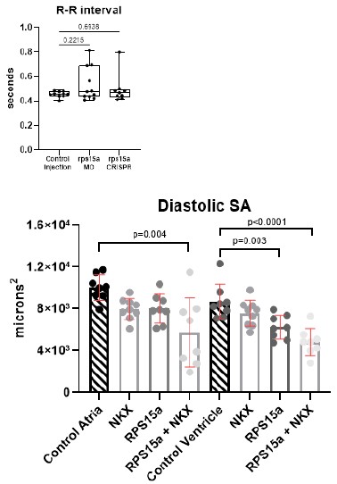
Finally, the use of the mouse to model HLHS in potential follow-up studies should be discussed.
We have added a mouse model comment to the discussion (lines 571-74): “In conclusion, we propose that the approach outlined in this study provides a novel framework for rapidly prioritizing candidate genes and systematically testing them, individually or in combination, using a CRISPR/Cas9 genome-editing strategy in mouse embryos (PMID: 28794185)”.
(6) When the authors scored proliferation in cells from the proband in family 75H, did they validate that RPS15A expression is reduced, consistent with a regulatory region defect?
Good point. We examined RPS15A expression in these cells and found no significant reduction in gene expression in day 25 cardiomyocytes (data not shown). One possible explanation is that this variant may regulate RPS15A expression in a stage-specific manner during differentiation or under additional stress conditions.
(7) Minor point. Typo on line 494: comma should be placed after KD, not before.
Thank you, this has now been corrected (new line 490)
Reviewer #2 (Recommendations for the authors):
(1) The authors are invited to revise the part of the manuscript that describes the genetic analysis and provide a more balanced discussion of the WGS data, with a conclusion that aligns with the strength of the human genetic data.
We disagree with reviewer #2’s assessment. The goal of our study is not to apply a classical genetic approach to establish variant pathogenicity, but rather to employ a multidisciplinary framework to prioritize candidate genes and variants and to examine their roles in heart development using model systems. In this context, genetic analysis serves primarily as a filtering tool rather than as a means of definitively establishing causality.
(2) The genetic analysis of patients does not appear to provide strong evidence for an association between RP gene variants and HLHS. More information regarding methodology and the identified variants is needed.
HLHS is widely recognized as an oligogenic and heterogeneous genetic disease in which traditional genetic analyses have consistently failed to prioritize any specific gene class as reviewer#2 is pointing out. Therefore, relying solely on genetic analysis is unlikely to yield strong evidence for association with a given gene class. This limitation provides the rationale for our multidisciplinary gene prioritization strategy, which leverages model systems to interrogate candidate gene function. Ultimately, definitive validation of this approach will require studies in relevant in vivo models to establish causality within the context of a four-chambered heart (see also Discussion).
In Table S2, it would be appropriate to provide information on sequence, MAF, and CADD. Please note the source of MAF% (GnomAD version?, which population?).
As summarized in Figure 2A, the 292 genes from the families with the 25 proband with poor outcome displayed in Supplemental Table 2 fulfilled a comprehensive candidate gene prioritization algorithm based on the variant, gene, inheritance, and enrichment, which required all of the following: 1) variants identified by whole genome sequencing with minor allele frequency <1%; 2) missense, loss-of-function, canonical splice, or promoter variants; 3) upper quartile fetal heart expression; and 4)De novo or recessive inheritance. Unbiased network analysis of these 292 genes, which are displayed in Supplemental Table 2 for completeness, identified statistically significant enrichment of ribosomal proteins. The details about MAF, CADD score, and sequence highlighted by the Reviewer are provided for the RP genes in Table 1, which are central to the focus and findings of the manuscript.
It would also be helpful for the reader if genome coordinates (e.g., 16-11851493-G-A for RSL1D1 p.A7V) were provided for each variant in both Table 1 and S2.
Genome coordinates have been added to Table 1.
(3) The dataset from the hPSC-CM screen could be of high value for the community. It would be appropriate if the complete dataset were made available in a usable format.
The dataset from the hPSC-CM screen has been added to the manuscript as Supp Table 1
(4) The "rare predicted-damaging promoter variant in RPS15A" (c.-95G>A) does not appear so rare. Considering the MAF of 0,00662, the frequency of heterozygous carriers of this variant is 1 out of 76 individuals in the general population. Thus, considering the frequency of HLHS in the population (2-3 out of 10,000) and the small size of family 75H, the data do not appear to indicate any association between this particular variant and HLHS. The variants in Table 1 also appear to have relatively mild effects on the gene product, judging from the MAF and CADD scores. The authors are invited to discuss why they find these variants disease-causing in HLHS.
Our study design is based on the widely held premise that HLHS is an oligogenic disorder. Our multi-model systems platform centered on comprehensive filtering of coding and regulatory variants identified by whole genome sequencing of HLHS probands to identify candidate genes associated with susceptibility to this rare developmental phenotype. 75H proved to be a high-value family for generating a relatively short list of candidate genes for left-sided CHD. Given the rarity of both left-sided CHD and the RPS15A variant identified in the HLHS proband and his 5th degree relative, with a frequency consistent with a risk allele for an oligogenic disorder, we made the reasonable assumption that this was a bona fide genotype-phenotype association rather than a chance occurrence. Moreover, incomplete penetrance and variable expression is consistent with a genetically complex basis of disease whereby the shared variant is risk-conferring and acts in conjunction with additional genetic, epigenetic, and/or environmental factors that lead to a left-sided CHD phenotype. In sum, we do not claim these variants are definitively disease causing, but rather potentially contributing risk factors.
(5) Information is lacking on how clustering of RP genes was demonstrated using STRING (with P-values that support the conclusions). What is meant by "when the highest stringency filter was applied"? Does this refer to the STRING interaction score or something else? The authors could also explain which genes were used to search STRING (e.g., all 292 candidate genes) and provide information on the STRING interaction score used in the analysis, the number of nodes and edges in the network.
To determine whether certain gene networks were over-represented, two online bioinformatics tools were used. First, genes were inputted into STRING (Author response table 2 below) to investigate experimental and predicted protein-protein and genetic interactions. Clustering of ribosomal protein genes was demonstrated when applying the highest stringency filter. Next, genes were analyzed for potential enrichment of genes by ontology classification using PANTHER .Applying Fisher’s exact test and false discovery rate corrections, ribosomal proteins were the most enriched class when compared to the reference proteome, including data annotated by molecular function (4.84-fold, p=0.02), protein class (6.45-fold, p=0.00001), and cellular component (9.50fold, p=0.001). A majority of the identified RP candidate genes harbored variants that fit a recessive inheritance disease model.
Author response image 2.

Synthèse du Débat : Le Genre Précède-t-il le Sexe ?
Ce document de synthèse analyse le débat contradictoire portant sur l'affirmation « Le genre précède le sexe », opposant Lou Girard (position affirmative) et Franck Ramus (position négative).
Le débat met en lumière une divergence fondamentale entre deux cadres d'analyse :
l'un, issu des études de genre et de la sociologie, postule que les structures sociales (le genre) façonnent la conceptualisation scientifique de la biologie (le sexe) ;
l'autre, ancré dans la biologie évolutionniste, soutient que les réalités biologiques (le sexe) constituent le substrat sur lequel se développent les constructions culturelles (le genre).
Lou Girard, s'appuyant sur les travaux de Christine Delphy et Thomas Laqueur, argue que la notion de sexe binaire est une construction scientifique récente (XVIIIe siècle), historiquement contingente et influencée par le système patriarcal qu'elle visait à justifier.
Pour Girard, le genre, en tant que système social hiérarchique, est donc premier.
Franck Ramus contre-argumente sur trois niveaux : ontologique (le phénomène biologique du sexe existe depuis un milliard d'années), développemental (un individu est sexué dès la conception, bien avant l'influence du genre) et évolutionniste (les différences de stratégies reproductives entre mâles et femelles expliquent l'émergence de rôles de genre récurrents dans les sociétés humaines).
La divergence principale ne réside pas seulement dans la conclusion, mais dans l'épistémologie :
quel poids accorder aux preuves issues de la sociologie historique par rapport à celles de la biologie évolutionniste ?
Le débat révèle que même lorsque les deux intervenants partagent des sources communes, leurs cadres interprétatifs radicalement différents les mènent à des conclusions opposées, notamment sur la nature binaire du sexe et la validité des reconstructions historiques des concepts scientifiques.
--------------------------------------------------------------------------------
Le débat a été organisé dans un format de "débat constructif" visant à clarifier les points d'accord et de désaccord plutôt qu'à déterminer un vainqueur.
Les deux intervenants ont été invités à défendre des positions opposées sur la proposition "Le genre précède le sexe".
• Position Affirmative ("Oui") : Défendue par Lou Girard.
• Position Négative ("Non") : Défendue par Franck Ramus.
Le format incluait des phases distinctes :
une prise de position initiale, une session de clarification pour assurer la compréhension mutuelle,
une phase de "personne de fer" où chaque intervenant reformulait la position de l'autre de manière charitable,
et des discussions sur les racines des convictions, les limites des approches respectives,
et enfin les points de convergence et de divergence.
La position de Lou Girard s'ancre dans le champ pluridisciplinaire des études sur le genre (sociologie, philosophie, études féministes).
Son argument central est que notre compréhension du "sexe" biologique est une construction sociale façonnée par le système de genre préexistant.
Origine et Définitions Clés
• Source de l'affirmation : La sociologue Christine Delphy.
• Définition du Genre : Un "système bicatégorisé (hommes/femmes) et hiérarchisé" où les femmes sont subordonnées aux hommes, notamment par l'exploitation de leur travail domestique et reproductif (patriarcat).
• Définition du Sexe : Il ne s'agit pas des organes génitaux, mais du concept de sexe tel qu'utilisé en biologie, c'est-à-dire la "distinction antagoniste entre les mâles et les femelles".
L'affirmation "Le genre précède le sexe" signifie que le concept scientifique du sexe biologique a été construit épistémologiquement sur les bases du patriarcat.
Il s'agit d'une "justification scientifique d'un système social".
La science n'a pas découvert le sexe binaire dans un vide neutre ; elle a formalisé une catégorie qui servait à rationaliser une organisation sociale déjà en place.
Girard s'appuie fortement sur les travaux de l'historien Thomas Laqueur (La fabrique du sexe) pour démontrer que la conception binaire du sexe est une idée récente.
• Avant le XVIIIe siècle : Le sexe n'était pas conçu comme deux catégories distinctes.
◦ Antiquité : Un modèle à "sexe unique" prévalait, où les organes féminins étaient vus comme une version invertie des organes masculins.
◦ Moyen Âge : Le sexe était perçu comme un continuum basé sur la "chaleur vitale", les hommes représentant le plus haut degré de cette chaleur.
• À partir du XVIIIe siècle : Le modèle binaire s'impose, coïncidant avec une volonté de naturaliser les rôles sociaux.
Le modèle binaire, une fois établi, a eu des conséquences concrètes, servant d'outil de normalisation sociale.
• Personnes intersexes : Plutôt que de remettre en question le modèle binaire face à des cas qui ne s'y conforment pas, la médecine a historiquement "mutilé" les personnes intersexes pour les faire correspondre à l'une des deux catégories.
• Homosexuels et personnes trans : Leur existence contrevenant au modèle biomédical, ils ont été psychiatrisés et internés.
• Biais actuel : Ce biais patriarcal continue, selon Girard, d'influencer la recherche scientifique, qui tend à justifier inconsciemment les normes patriarcales plutôt qu'à décrire les faits de manière neutre.
La position de Franck Ramus repose sur une distinction claire entre le phénomène biologique du sexe et le concept humain de sexe.
Il soutient que le sexe, en tant que réalité biologique fondamentale, précède et influence l'émergence des constructions sociales comme le genre.
• Le Sexe comme Stratégie Reproductive : Ramus définit le sexe à son niveau le plus fondamental, stabilisé en biologie, comme la distinction entre deux types sexuels dans la reproduction sexuée anisogame :
◦ Femelles : Porteurs de gros gamètes (ovocytes). ◦ Mâles : Porteurs de petits gamètes (spermatozoïdes).
• Cette définition est primordiale, et les autres aspects (génétiques, hormonaux) en découlent.
Ramus défend que le sexe précède le genre à trois échelles distinctes :
1. Niveau Ontologique : Le phénomène du sexe existe dans la nature depuis environ un milliard d'années, bien avant l'apparition de l'humanité, du patriarcat ou de la conceptualisation humaine du sexe.
2. Niveau Développemental (Individuel) : Un individu possède un sexe dès la conception (chromosomes sexuels).
L'influence du genre et des représentations sociales n'intervient qu'après la naissance. Pour le fœtus, le sexe précède donc clairement le genre.
3. Niveau Évolutionniste (Espèce) : Le genre, en tant que phénomène social, n'émerge pas de rien.
Il se développe sur la base de prédispositions biologiques issues de l'évolution.
Ramus propose une explication évolutionniste à l'origine des rôles de genre.
• Investissement Parental Différentiel : L'anisogamie (différence de taille des gamètes) entraîne un investissement reproductif initial plus élevé pour les femelles.
Cela les incite à investir davantage dans la survie de la progéniture (gestation, allaitement, élevage).
L'investissement des mâles peut rester minimal.
• Conséquences Comportementales :
◦ Les mâles sont en compétition pour l'accès aux femelles, ce qui sélectionne des traits comme l'agressivité, la taille et la force.
◦ Les femelles, ayant plus à perdre, sont plus sélectives dans le choix de leurs partenaires.
• Origine de la Domination Masculine : La sélection pour une plus grande taille et force chez les mâles (pour la compétition inter-mâles) a pour "effet secondaire" de les rendre physiquement plus forts que les femelles, rendant ainsi la domination masculine possible.
• Division du Travail : Les contraintes reproductives (grossesse, allaitement) rendent les femelles plus sédentaires, tandis que les mâles sont plus mobiles.
Cela favorise une "répartition relativement naturelle des rôles et des tâches", que l'on retrouve dans de multiples cultures.
Ramus précise que ce n'est pas une justification morale, mais une explication causale.
Le débat a cristallisé plusieurs points de désaccord profonds, qui sont moins factuels qu'épistémologiques.
C'est l'opposition centrale du débat.
• Pour Girard : La culture précède la nature. Les systèmes sociaux (genre) déterminent la manière dont nous conceptualisons et même percevons la réalité biologique (sexe).
• Pour Ramus : La nature précède la culture. Les prédispositions biologiques humaines constituent le socle sur lequel les cultures se développent.
• Pour Ramus : Le sexe, défini par la stratégie reproductive (production de deux types de gamètes), est fondamentalement binaire.
• Pour Girard : Le sexe biologique n'est pas binaire. Cette vision est le produit d'un modèle social imposé à une réalité plus complexe (comme en témoignent les personnes intersexes).
Le cas de Thomas Laqueur est emblématique de cette divergence.
• Girard accepte les conclusions de Laqueur comme une preuve historique valide que la conception binaire du sexe est une construction récente.
• Ramus exprime son "incrédulité" face à cette affirmation, la trouvant contre-intuitive.
Il a du mal à imaginer qu'avant le XVIIIe siècle, les humains n'avaient pas conscience de l'existence de deux sexes.
Pour lui, le critère d'arbitrage serait le consensus scientifique parmi les historiens, pas la thèse d'un seul auteur.
Poids Épistémologique des Disciplines et des Données
Initialement présentée comme une opposition entre sociologie (Girard) et biologie (Ramus), la divergence est plus subtile.
• Girard accorde une grande valeur aux analyses des études de genre pour déconstruire les biais inhérents à la production du savoir scientifique.
• Ramus ne rejette pas les sciences humaines et sociales, mais se dit "non convaincu" par certains arguments et données spécifiques issus des études de genre, qu'il confronte à des données issues de la biologie ou de la psychologie.
Le débat a montré que même en lisant les mêmes auteurs (ex: Anne Fausto-Sterling), ils en tirent des conclusions radicalement opposées, révélant des cadres d'analyse irréconciliables.
• Franck Ramus : Son intérêt pour le sujet provient de ses recherches en sciences cognitives, où il a observé de manière répétée et non sollicitée des différences entre sexes (prévalence de l'autisme, dyslexie, développement du langage, neuroanatomie), le poussant à en chercher les origines.
• Lou Girard : Sa position est façonnée par son expérience de femme transgenre.
La confrontation au sexisme et à la transphobie l'a conduite à s'intéresser au féminisme, puis aux études de genre, dont elle a adopté le cadre d'analyse matérialiste comme étant le plus pertinent pour comprendre la société.
• Franck Ramus : Admet que l'approche évolutionniste est une "inférence à la meilleure explication" et qu'il ne peut apporter de "preuves irréfutables" pour chaque détail de ce récit historique.
Sa force réside dans sa cohérence et son pouvoir explicatif global.
• Lou Girard : Reconnaît ses limites personnelles en tant que non-experte diplômée, ce qui pourrait limiter sa compréhension des théories qu'elle expose.
Elle admet également la possibilité de faiblesses épistémologiques dans l'approche des études de genre elle-même, ainsi que l'existence de limites qu'elle ne perçoit pas.
Malgré les divergences profondes, quelques points d'accord ont été établis :
• L'existence du patriarcat en tant que système social qui désavantage les femmes.
• La préexistence de phénomènes biologiques ("nature") avant l'émergence de la culture humaine.
• Le fait que les individus sont biologiquement sexués avant d'être socialisés.
• Un désaccord commun sur la validité du premier modèle des "cinq sexes" d'Anne Fausto-Sterling, bien que leur analyse de l'évolution de son travail diverge par la suite.
Author response:
The following is the authors’ response to the original reviews.
Reviewer #1 (Public review):
“The study analyzes the gastric fluid DNA content identified as a potential biomarker for human gastric cancer. However, the study lacks overall logicality, and several key issues require improvement and clarification. In the opinion of this reviewer, some major revisions are needed:”
(1) “This manuscript lacks a comparison of gastric cancer patients' stages with PN and N+PD patients, especially T0-T2 patients.”
We are grateful for this astute remark. A comparison of gfDNA concentration among the diagnostic groups indicates a trend of increasing values as the diagnosis progresses toward malignancy. The observed values for the diagnostic groups are as follows:
Author response table 1.

The chart below presents the statistical analyses of the same diagnostic/tumor-stage groups (One-Way ANOVA followed by Tukey’s multiple comparison tests). It shows that gastric fluid gfDNA concentrations gradually increase with malignant progression. We observed that the initial tumor stages (T0 to T2) exhibit intermediate gfDNA levels, which in this group is significantly lower than in advanced disease (p = 0.0036), but not statistically different from non-neoplastic disease (p = 0.74).
Author response image 1.
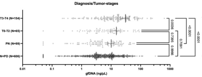
(2) “The comparison between gastric cancer stages seems only to reveal the difference between T3 patients and early-stage gastric cancer patients, which raises doubts about the authenticity of the previous differences between gastric cancer patients and normal patients, whether it is only due to the higher number of T3 patients.”
We appreciate the attention to detail regarding the numbers analyzed in the manuscript. Importantly, the results are meaningful because the number of subjects in each group is comparable (T0-T2, N = 65; T3, N = 91; T4, N = 63). The mean gastric fluid gfDNA values (ng/µL) increase with disease stage (T0-T2: 15.12; T3-T4: 30.75), and both are higher than the mean gfDNA values observed in non-neoplastic disease (10.81 ng/µL for N+PD and 10.10 ng/µL for PN). These subject numbers in each diagnostic group accurately reflect real-world data from a tertiary cancer center.
(3) “The prognosis evaluation is too simplistic, only considering staging factors, without taking into account other factors such as tumor pathology and the time from onset to tumor detection.”
Histopathological analyses were performed throughout the study not only for the initial diagnosis of tissue biopsies, but also for the classification of Lauren’s subtypes, tumor staging, and the assessment of the presence and extent of immune cell infiltrates. Regarding the time of disease onset, this variable is inherently unknown--by definition--at the time of a diagnostic EGD. While the prognosis definition is indeed straightforward, we believe that a simple, cost-effective, and practical approach is advantageous for patients across diverse clinical settings and is more likely to be effectively integrated into routine EGD practice.
(4) “The comparison between gfDNA and conventional pathological examination methods should be mentioned, reflecting advantages such as accuracy and patient comfort. “
We wish to reinforce that EGD, along with conventional histopathology, remains the gold standard for gastric cancer evaluation. EGD under sedation is routinely performed for diagnosis, and the collection of gastric fluids for gfDNA evaluation does not affect patient comfort. Thus, while gfDNA analysis was evidently not intended as a diagnostic EGD and biopsy replacement, it may provide added prognostic value to this exam.
(5) “There are many questions in the figures and tables. Please match the Title, Figure legends, Footnote, Alphabetic order, etc. “
We are grateful for these comments and apologize for the clerical oversight. All figures, tables, titles and figure legends have now been double-checked.
(6) “The overall logicality of the manuscript is not rigorous enough, with few discussion factors, and cannot represent the conclusions drawn. “
We assume that the unusual wording remark regarding “overall logicality” pertains to the rationale and/or reasoning of this investigational study. Our working hypothesis was that during neoplastic disease progression, tumor cells continuously proliferate and, depending on various factors, attract immune cell infiltrates. Consequently, both tumor cells and immune cells (as well as tumor-derived DNA) are released into the fluids surrounding the tumor at its various locations, including blood, urine, saliva, gastric fluids, and others. Thus, increases in DNA levels within some of these fluids have been documented and are clinically meaningful. The concurrent observation of elevated gastric fluid gfDNA levels and immune cell infiltration supports the hypothesis that increased gfDNA—which may originate not only from tumor cells but also from immune cells—could be associated with better prognosis, as suggested by this study of a large real-world patient cohort.
In summary, we thank Reviewer #1 for his time and effort in a constructive critique of our work.
Reviewer #2 (Public review):
Summary:
“The authors investigated whether the total DNA concentration in gastric fluid (gfDNA), collected via routine esophagogastroduodenoscopy (EGD), could serve as a diagnostic and prognostic biomarker for gastric cancer. In a large patient cohort (initial n=1,056; analyzed n=941), they found that gfDNA levels were significantly higher in gastric cancer patients compared to non-cancer, gastritis, and precancerous lesion groups. Unexpectedly, higher gfDNA concentrations were also significantly associated with better survival prognosis and positively correlated with immune cell infiltration. The authors proposed that gfDNA may reflect both tumor burden and immune activity, potentially serving as a cost-effective and convenient liquid biopsy tool to assist in gastric cancer diagnosis, staging, and follow-up.”
Strengths:
“This study is supported by a robust sample size (n=941) with clear patient classification, enabling reliable statistical analysis. It employs a simple, low-threshold method for measuring total gfDNA, making it suitable for large-scale clinical use. Clinical confounders, including age, sex, BMI, gastric fluid pH, and PPI use, were systematically controlled. The findings demonstrate both diagnostic and prognostic value of gfDNA, as its concentration can help distinguish gastric cancer patients and correlates with tumor progression and survival. Additionally, preliminary mechanistic data reveal a significant association between elevated gfDNA levels and increased immune cell infiltration in tumors (p=0.001).”
Reviewer #2 has conceptually grasped the overall rationale of the study quite well, and we are grateful for their assessment and comprehensive summary of our findings.
Weaknesses:
(1) “The study has several notable weaknesses. The association between high gfDNA levels and better survival contradicts conventional expectations and raises concerns about the biological interpretation of the findings.“
We agree that this would be the case if the gfDNA was derived solely from tumor cells. However, the findings presented here suggest that a fraction of this DNA would be indeed derived from infiltrating immune cells. The precise determination of the origin of this increased gfDNA remains to be achieved in future follow-up studies, and these are planned to be evaluated soon, by applying DNA- and RNA-sequencing methodologies and deconvolution analyses.
(2) “The diagnostic performance of gfDNA alone was only moderate, and the study did not explore potential improvements through combination with established biomarkers. Methodological limitations include a lack of control for pre-analytical variables, the absence of longitudinal data, and imbalanced group sizes, which may affect the robustness and generalizability of the results.“
Reviewer #2 is correct that this investigational study was not designed to assess the diagnostic potential of gfDNA. Instead, its primary contribution is to provide useful prognostic information. In this regard, we have not yet explored combining gfDNA with other clinically well-established diagnostic biomarkers. We do acknowledge this current limitation as a logical follow-up that must be investigated in the near future.
Moreover, we collected a substantial number of pre-analytical variables within the limitations of a study involving over 1,000 subjects. Longitudinal samples and data were not analyzed here, as our aim was to evaluate prognostic value at diagnosis. Although the groups are imbalanced, this accurately reflects the real-world population of a large endoscopy center within a dedicated cancer facility. Subjects were invited to participate and enter the study before sedation for the diagnostic EGD procedure; thus, samples were collected prospectively from all consenting individuals.
Finally, to maintain a large, unbiased cohort, we did not attempt to balance the groups, allowing analysis of samples and data from all patients with compatible diagnoses (please see Results: Patient groups and diagnoses).
(3) “Additionally, key methodological details were insufficiently reported, and the ROC analysis lacked comprehensive performance metrics, limiting the study's clinical applicability.“
We are grateful for this useful suggestion. In the current version, each ROC curve (Supplementary Figures 1A and 1B) now includes the top 10 gfDNA thresholds, along with their corresponding sensitivity and specificity values (please see Suppl. Table 1). The thresholds are ordered from-best-to-worst based on the classic Youden’s J statistic, as follows:
Youden Index = specificity + sensitivity – 1 [Youden WJ. Index for rating diagnostic tests. Cancer 3:32-35, 1950. PMID: 15405679]. We have made an effort to provide all the key methodological details requested, but we would be glad to add further information upon specific request.
Reviewer #1 (Recommendations for the authors):
The authors should pay attention to ensuring uniformity in the format of all cited references, such as the number of authors for each reference, the journal names, publication years, volume numbers, and page number formats, to the best extent possible.
Thank you for pointing this inconsistency. All cited references have now been revisited and adjusted properly. We apologize for this clerical oversight.
Reviewer #2 (Recommendations for the authors):
(1) “High gfDNA levels were surprisingly linked to better survival, which conflicts with the conventional understanding of cfDNA as a tumor burden marker. Was any qualitative analysis performed to distinguish DNA derived from immune cells versus tumor cells?“
Tumor-derived DNA is certainly present in gfDNA, as our group has unequivocally demonstrated in a previous publication [Pizzi M. P., et al. (2019) Identification of DNA mutations in gastric washes from gastric adenocarcinoma patients: Possible implications for liquid biopsies and patient follow-up Int J Cancer 145:1090–1097. DOI: 10.1002/ijc.32114]. However, in the present manuscript, our data suggest that gfDNA may also contain DNA derived from infiltrating immune cells. This may also be the case for other malignancies, and qualitative deconvolution studies could provide more informative information. To achieve this, DNA sequencing and RNA-Seq analyses may offer relevant evidence. Our study should be viewed as an original and preliminary analysis that may encourage such quantitative and qualitative studies in biofluids from cancer patients. Currently, this is a simple approach (which might be its essential beauty), but we hope to investigate this aspect further in future studies.
(2) “The ROC curve AUC was 0.66, indicating only moderate discrimination ability. Did the authors consider combining gfDNA with markers such as CEA or CA19-9 to improve diagnostic accuracy?“
This is indeed a logical idea, which shall certainly be explored in planned follow-up studies.
(3) “DNA concentration could be influenced by non-biological factors, including gastric fluid pH, sampling location, time delay, or freeze-thaw cycles. Were these operational variables assessed for their effect on data stability?“
We appreciate the rigor of the evaluation. Yes, information regarding gastric fluid pH was collected. All samples were collected from the stomach during EGD procedure. Samples were divided in aliquots and were thawed only once. This information is now provided in the updated manuscript text.
(4) “This cross-sectional study lacks data on gfDNA changes over time, limiting conclusions on its utility for monitoring treatment response or predicting recurrence.“
Again, temporal evaluation is another excellent point, and it will be the subject of future analyses. In this exploratory study, samples were collected at diagnosis, at a single point. We have not obtained serial samples, as participants received appropriate therapy soon following diagnosis.
(5) The normal endoscopy group included only 10 patients, the precancerous lesion group 99 patients, while the gastritis group had 596 patients. Such uneven sample sizes may affect statistical reliability and generalizability. Has weighted analysis or optimized sampling been considered for future studies?“
Yes, in future studies this analysis will be considered, probably by employing stratified random sampling with relevant patient attributes recorded.
(6) “The SciScore was only 2 points, indicating that key methodological details such as inclusion/exclusion criteria, randomization, sex variables, and power calculation were not clearly described. It is recommended that these basic research elements be supplemented in the Methods section. “
This was an exploratory research, the first of its kind, to evaluate prognostic potential of gfDNA in the context of gastric cancer. Patients were not included if they did not sign the informed consent or excluded if they withdrew after consenting. Other exclusion criteria included diagnoses of conditions such as previous gastrectomy or esophagectomy, or the presence of non-gastric malignancies. Randomization and power analyses were not applicable, as no prior data were available regarding gfDNA concentration values or its diagnostic/prognostic potential. All subjects, regardless of sex, were invited to participate without discrimination or selection.
(7) “Although a ROC curve was provided in the supplementary materials (Supplementary Figure 1), only the curve and AUC value were shown without sensitivity, specificity, predictive values, or cutoff thresholds. The authors are advised to provide a full ROC performance assessment to strengthen the study's clinical relevance.
These data are now given alongside the ROC curves in the Supplementary Information section, specifically in Supplementary Figure 1 and in the newly added Supplementary Table 1.
We thank Reviewer #2 for an insightful and positive overall assessment of our work.
L'Idéologie et l'Esprit Critique : Synthèse du Débat
Ce document synthétise les arguments et les conclusions du débat sur la compatibilité entre l'idéologie et l'esprit critique, opposant Gwen Pallarès (position positive) et Pascal Wagner-Egger (position négative).
Gwen Pallarès soutient que l'idéologie est non seulement compatible mais souvent un prérequis et un moteur pour l'esprit critique, arguant que tout individu possède une idéologie qui structure sa pensée et motive sa curiosité.
Pascal Wagner-Egger défend la position selon laquelle l'idéologie est fondamentalement un obstacle à la pensée critique et à la démarche scientifique, un ensemble de préconceptions qu'il faut activement chercher à minimiser en s'appuyant sur des données empiriques.
Malgré leurs positions de départ opposées, un consensus significatif a émergé sur plusieurs points.
Les deux intervenants s'accordent sur l'existence d'un "point de bascule" ou d'un "saut qualitatif" où l'idéologie devient incompatible avec l'esprit critique, notamment dans les cas de fanatisme, de radicalisation ou lorsque les croyances fondamentales liées à l'identité sont menacées.
Ils reconnaissent également que l'idéologie peut agir comme une puissante "motivation épistémique", incitant à la recherche et à l'analyse.
La divergence principale réside dans la nature de cette relation.
Pour Pascal, la motivation induite par l'idéologie est une arme à double tranchant qui exige une vigilance épistémique accrue pour contrer les biais.
Pour Gwen, cette motivation est un moteur fondamental, et la volonté de se placer dans une position "centriste" pour éviter les biais est elle-même une position idéologique.
Cette différence de perspective trouve sa source dans des divergences épistémologiques plus profondes sur la nature des sciences, la construction des données et la porosité entre les domaines scientifique et politique.
Le débat, animé par Peter Barret, a pour objectif d'explorer la question "L’idéologie est-elle compatible avec l’esprit critique ?" dans un format visant à être constructif et à clarifier les positions plutôt qu'à encourager la contre-argumentation.
Les deux intervenants sont :
• Gwen Pallarès : Maîtresse de conférence en didactique des sciences à l'Université de Reims Champagne-Ardenne, défendant la position positive.
• Pascal Wagner-Egger : Psychologue social à l'Université de Fribourg, défendant la position négative.
Les intervenants se sont accordés sur les définitions suivantes pour encadrer le débat.
Terme
Définition de Gwen Pallarès (Psychologie Sociale)
Définition de Pascal Wagner-Egger (Larousse)
Idéologie
Un système d'attitudes, de croyances et de stéréotypes qui coordonne les actions des institutions et des individus.
Ce système vise notamment à justifier ou à critiquer les hiérarchies sociales existantes (ex: féminisme vs. masculinisme).
Un système d'idées générales constituant un corps de doctrine philosophique et politique à la base d'un comportement individuel ou collectif (ex: idéologie marxiste, nationaliste).
Esprit Critique : Défini par Gwen Pallarès comme un ensemble de compétences (analyse, évaluation d'arguments et d'informations) et de dispositions (humilité intellectuelle, curiosité, réflexivité).
Cet ensemble est orienté vers la prise de décision raisonnée ("Qu'est-ce qu'il convient de croire ou de faire ?") et s'opérationnalise souvent par une argumentation de bonne qualité.
L'argument central de Gwen Pallarès repose sur l'universalité de l'idéologie :
• Tout le monde a une idéologie : La pensée de chaque individu est structurée par des systèmes de croyances, d'attitudes et de stéréotypes.
Refuser cela serait nier une réalité fondamentale du fonctionnement humain.
• L'incompatibilité rendrait l'esprit critique impossible : Si l'idéologie était incompatible avec l'esprit critique, et puisque tout le monde a une idéologie, alors personne ne pourrait avoir d'esprit critique.
• L'esprit critique est un spectre : Tout le monde possède des compétences minimales d'analyse et d'argumentation, même si leur application peut être biaisée (ex: biais de confirmation où l'on critique plus durement les informations qui contredisent nos croyances).
• Limite de la compatibilité : Elle concède que les formes extrêmes d'idéologie (radicalisation, emprise sectaire, fanatisme) sont, elles, incompatibles avec l'esprit critique car elles poussent à une acceptation acritique des informations.
Pascal Wagner-Egger ancre sa position dans l'histoire des sciences et la psychologie sociale :
• La science s'est construite contre l'idéologie : Il cite l'exemple de la science luttant contre l'idéologie religieuse, qu'il qualifie de "régime totalitaire".
• La "méthode idéologique" : Elle postule que la vérité est contenue dans un texte fondateur (la Bible, Le Capital) et que toute observation doit s'y conformer. C'est l'inverse de la méthode scientifique.
• L'ennemi intérieur et extérieur : L'idéologie est un obstacle institutionnel (externe) mais aussi un obstacle interne aux chercheurs eux-mêmes.
Il cite Gaston Bachelard et ses "obstacles épistémologiques" (opinion, connaissance générale) comme précurseurs de la notion de biais cognitifs.
• Le rôle des données empiriques : La méthode scientifique est le principal outil pour limiter les effets de nos idéologies et tester nos préconceptions contre la réalité.
Il cite des études montrant plus de dogmatisme et de complotisme aux extrêmes politiques.
Les positions des deux débatteurs sont fortement influencées par leurs expériences personnelles et académiques.
• Pascal Wagner-Egger : Son parcours l'a mené des sciences "dures" vers les sciences sociales.
Il a été frappé par ce qu'il a perçu comme des positions idéologiques dogmatiques chez certains collègues, notamment le rejet des méthodes quantitatives qualifiées d'"impérialisme anglo-saxon".
Cette expérience a forgé sa conviction que l'idéologie peut nuire à la recherche de la vérité scientifique et qu'il faut s'en prémunir.
• Gwen Pallarès : Son parcours est inverse, des mathématiques vers la didactique des sciences.
L'étude approfondie des controverses socio-scientifiques (IA, genre, écologie) pour sa thèse l'a progressivement politisée.
Son engagement politique est devenu un moteur pour produire une recherche scientifique plus rigoureuse et utile socialement, notamment pour l'éducation.
Pour elle, l'idéologie n'est pas un obstacle à la rigueur, mais ce qui la motive.
Le débat a révélé un terrain d'entente plus large qu'attendu, tout en précisant la nature des désaccords.
1. Le "Point de Bascule" : Les deux intervenants s'accordent sur le fait qu'il existe un seuil où l'idéologie devient incompatible avec l'esprit critique.
Ce seuil est atteint dans les cas de fanatisme, de radicalisation, ou lorsque des croyances fondamentales liées à l'identité de la personne sont menacées, rendant le dialogue et la remise en question impossibles.
2. La Motivation Épistémique : Il est admis par les deux parties que l'idéologie est un puissant moteur.
Un engagement idéologique (ex: écologiste, féministe) peut stimuler la curiosité intellectuelle, la recherche d'informations et la volonté d'analyser des arguments, qui sont des dispositions centrales de l'esprit critique.
3. L'Universalité de l'Idéologie : Les deux débatteurs partagent le postulat que chaque individu, y compris les scientifiques, possède une ou plusieurs idéologies qui structurent sa vision du monde.
La principale divergence ne porte pas tant sur la compatibilité en soi, mais sur la nature de la relation entre idéologie et esprit critique.
Point de Divergence
Position de Pascal Wagner-Egger
Position de Gwen Pallarès
Nature du lien
Une arme à double tranchant : L'idéologie motive, mais elle biaise simultanément.
Il est donc crucial d'exercer une vigilance épistémique accrue et de chercher à minimiser l'influence de ses propres idéologies, notamment en les confrontant aux données empiriques.
Un moteur fondamental : L'idéologie est le moteur principal de la recherche et de l'engagement critique. Tenter de l'annuler est illusoire.
La posture qui consiste à se vouloir "au centre" pour être moins biaisé est elle-même une idéologie ("biais du juste milieu").
Épistémologie sous-jacente
Plus proche de l'empirisme et du rationalisme critique (citant Popper et se revendiquant de Lakatos).
Les données, bien que partiellement construites, permettent par triangulation de s'approcher d'une réalité indépendante de la méthode.
Plus proche du constructivisme et du pragmatisme. Les données sont fondamentalement construites par la méthodologie, qui est elle-même issue de cadres théoriques.
La distinction entre science et politique est plus poreuse.
Rapport Science / Politique
Vise à maintenir une distinction claire. Dans le domaine scientifique, les données doivent primer sur les préconceptions. Dans le domaine politique, l'idéologie et le militantisme sont utiles et nécessaires.
La distinction est moins nette. Le travail scientifique est intrinsèquement lié à des enjeux de société et peut être motivé par un engagement politique, cet engagement pouvant être un gage de rigueur pour rendre la science utile.
En tout cas, vous pouvez aller tester ces différentes propriétés et vous amuser à recréer l'élément ci-dessus avec le CodePen P2C4a.
bonjour, j'ai une preoccupation et elle est la suivante : je suis aller dans cette section de code pen j'ai constaté que les valeurs attribuées à l'attribu class ne sont declarées de la meme maniére dans le css. et j'aimerai comprendre pourquoi s'il vous plait.
aussi j'aimerai comprendre si Box apres l'espace dans le HTML lors de l'affectation des valeurs à l'attribut veut tout simplement dire que l'on aura des valeurs geometriques comme par exemple un carré et donc c'est la raison pour laquelle il ne figure pas dans le CSS. merci d'avance pour votre orientation
Note: This response was posted by the corresponding author to Review Commons. The content has not been altered except for formatting.
Learn more at Review Commons
Manuscript number: RC -2025-03175
Corresponding author(s): Gernot Längst
[Please use this template only if the submitted manuscript should be considered by the affiliate journal as a full revision in response to the points raised by the reviewers.
If you wish to submit a preliminary revision with a revision plan, please use our "Revision Plan" template. It is important to use the appropriate template to clearly inform the editors of your intentions.]
This section is optional. Insert here any general statements you wish to make about the goal of the study or about the reviews.
This section is mandatory. *Please insert a point-by-point reply describing the revisions that were already carried out and included in the transferred manuscript. *
We thank the reviewers for their efforts and detailed evaluation of our manuscript. We think that the comments of the reviewers allowed us to significantly improve the manuscript.
With best regards
The authors of the manuscript
Reviewer #1 (Evidence, reproducibility and clarity (Required)):
Summary: Holzinger et al. present a new automated pipeline, nucDetective, designed to provide accurate nucleosome positioning, fuzziness, and regularity from MNase-seq data. The pipeline is structured around two main workflows-Profiler and Inspector-and can also be applied to time-series datasets. To demonstrate its utility, the authors re-analyzed a Plasmodium falciparum MNase-seq time-series dataset (Kensche et al., 2016), aiming to show that nucDetective can reliably characterize nucleosomes in challenging AT-rich genomes. By integrating additional datasets (ATAC-seq, RNA-seq, ChIP-seq), they argue that the nucleosome positioning results from their pipeline have biological relevance.
Major Comments:
Despite being a useful pipeline, the authors draw conclusions directly from the pipeline's output without integrating necessary quality controls. Some claims either contradict existing literature or rely on misinterpretation or insufficient statistical support. In some instances, the pipeline output does not align with known aspects of Plasmodium biology. I outline below the key concerns and suggested improvements to strengthen the manuscript and validate the pipeline:
Clarification of +1 Nucleosome Positioning in P. falciparum The authors should acknowledge that +1 nucleosomes have been previously reported in P. falciparum. For example, Kensche et al. (2016) used MNase-seq to map ~2,278 TSSs (based on enriched 5′-end RNA data) and found that the +1 nucleosome is positioned directly over the TSS in most genes:
"Analysis of 2278 start sites uncovered positioning of a +1 nucleosome right over the TSS in almost all analysed regions" (Figure 3A).
They also described a nucleosome-depleted region (NDR) upstream of the TSS, which varies in size, while the +1 nucleosome frequently overlaps the TSS. The authors should nuance their claims accordingly. Nevertheless, I do agree that the +1 positioning in P. falciparum may be fuzzier as compared to yeast or mammals. Moreover, the correlation between +1 nucleosome occupancy and gene expression is often weak and that several genes show similar nucleosome profiles regardless of expression level. This raises my question: did the authors observe any of these patterns in their new data?
We appreciate the reviewer’s insightful comment and agree that +1 nucleosomes and nucleosome depleted promoter regions have been previously reported in P. falciparum, notably by the Bartfai and Le Roch groups, including Kensche et al. (PMID: 26578577). Our study advances this understanding by providing, for the first time, a comprehensive view of the entirety of a canonical eukaryotic promoter architecture in P. falciparum—encompassing the NDR, the well-positioned +1 nucleosome, and the downstream phased nucleosome array. This downstream nucleosome array structure has not been characterized before, as prior studies noted a “lack of downstream nucleosomal arrays” (PMID: 26578577) or “relatively random” nucleosome organization within gene bodies (PMID: 24885191). We have revised the manuscript to more clearly acknowledge previous work and highlight our contributions. The changes we applied in the manuscript are highlighted in yellow and shown as well below.
In the Abstract L26-L230: Contrary to the current view of irregular chromatin, we demonstrate for the first time regular phased nucleosome arrays downstream of TSSs, which, together with the established +1 nucleosome and upstream nucleosome-depleted region, reveal a complete canonical eukaryotic promoter architecture in Pf.
Introduction L156-L159: For example, we identify a phased nucleosome array downstream of the TSS. Together with a well-positioned +1 nucleosome and an upstream nucleosome-free region. These findings support a promoter architecture in Pf that resembles classical eukaryotic promoters (Bunnik et al. 2014, Kensche et al. 2016).
Results L181-L183: These new Pf nucleosome maps reveal a nucleosome organisation at transcription start sites (TSS) reminiscent of the general eukaryotic chromatin structure, featuring a reported well-positioned +1 nucleosome , an upstream nucleosome-free region (NFR, Bunnik et al. 2014, Kensche et al. 2016), and shown for the first time in Pf, a phased nucleosome array downstream of the TSS.
Discussion L414-L419: Previous analyses of Pf chromatin have identified +1 nucleosomes and NFRs (Bunnik et al 2014, Kensche et al. 2016). Here we extend this understanding by demonstrating phased nucleosome array structures throughout the genome. This finding provides evidence for a spatial regulation of nucleosome positioning in Pf, challenging the notion that nucleosome positioning is relatively random in gene bodies (Bunnik et al. 2014, Kensche et al. 2016). Consequently our results contribute to the understanding that Pf exhibits a typical eukaryotic chromatin structure, including well-defined nucleosome positioning at the TSS and regularly spaced nucleosome arrays (Schones et al. 2008; Yuan et al. 2005).
Regarding the reviewer’s question on +1 nucleosome dynamics. Our data agrees with the reviewer and other studies (e.g. PMID: 31694866), that the +1 nucleosome position is robust and does not correlate with gene expression strength. In the manuscript we show that dynamic nucleosomes are preferentially detected at the –1 nucleosome position (Figure 2C). In line with that we show that the +1 nucleosome position does not markedly change during transcription initiation of a subset of late transcribed genes (Figure 5A). However, we observe an opening of the NDR and within the gene body increased fuzziness and decreased nucleosome array regularity (Figure S4A). To illustrate the relationship between the +1 nucleosome positioning and expression strength, we have included a heatmap showing nucleosome occupancy at the TSS, ordered according to expression strength (NEW Figure S4C):
We included a sentence describing the relationship of +1 nucleosome position with gene expression in L257-L258: Furthermore, the +1 nucleosome positioning is unaffected by the strength of gene expression (Figure S2C).
__ Lack of Quality Control in the Pipeline __
The authors claim (lines 152-153) that QC is performed at every stage, but this is not supported by the implementation. On the GitHub page (GitHub - uschwartz/nucDetective), QC steps are only marked at the Profiler stage using standard tools (FastQC, MultiQC). The Inspector stage, which is crucial for validating nucleosome detection, lacks QC entirely. The authors should implement additional steps to assess the quality of nucleosome calls. For example, how are false positives managed? ROC curves should be used to evaluate true positive vs. false positive rates when defining dynamic nucleosomes. How sequencing biases are adressed?
The workflow overview chart on GitHub was not properly color coded. Therefore, we changed the graphics and highlighted the QC steps in the overview charts accordingly:
Based on our long standing expertise of analysing MNase-seq data (PMID: 38959309, PMID: 37641864, PMID: 30496478, PMID: 25608606), the best quality metrics to assess the performance of the challenging MNase experiment are the fragment size distributions revealing the typical nucleosomal DNA lengths and the TSS plots showing a positioned +1 nucleosome and regularly phased nucleosome arrays downstream of the +1 nucleosome. Additionally, visual inspection of the nucleosome profiles in a genome browser is advisable. We make those quality metrics easily available in the nucDetective Profiler workflow (Insertsize Histogram, TSS plot and provide nucleosome profile bigwig files). Furthermore, the PC and correlation analysis based on the nucleosome occupancy in the inspector workflow allows to evaluate replicate reproducibility or integrity of time series data, as shown for data evaluated in this manuscript.
The inspector workflow uses the well-established DANPOS toolkit to call nucleosome positions. Based on our experience, this step is particularly robust and well-established in the DANPOS toolkit (PMID: 23193179), so there is no need to reinvent it. Nevertheless, appropriate pre-processing of the data as done in the nucDetective pipeline is crucial to obtain highly resolved nucleosome positions. Using the final nucleosome profiles (bigwig) and the nucleosome reference positions (bed) as output of the Inspector workflow allows visual inspection of the called nucleosomes in a genome viewer. Furthermore, to avoid using false positive nucleosome positions for dynamic nucleosome analysis, we take only the 20% best positioned nucleosomes of each sample, as determined by the fuzziness score.
We understand the value of a gold standard of dynamic nucleosomes to test performance using ROC curves. However, we are not aware that such a gold standard exists in the nucleosome analysis field, especially not when using multi-sample settings, such as time series data. One alternative would be to use simulated data; however, this has several limitations:
Poor Model Fidelity and Hidden Assumptions: The authenticity of simulated data is bounded by the fidelity of the underlying models. If those models are inaccurate or make untested assumptions, the generated data may not reflect real experimental or clinical scenarios. This can mask software shortcomings or bias validation toward specific, perhaps irrelevant, scenarios. Therefore, we decided to validate the performance of the pipeline in the biological context of the analyzed data:
PCA analysis of the individual nucleosome features shows a cyclic structure as expected for the IDC (Fig. 1D-G).
We included a paragraph describing the limitations to the discussion (L447-457):
Depending on the degree of MNase digestion, preferentially nucleosomes from GC rich regions are revealed in MNase-seq experiments (Schwartz et al. 2019). However, no sequence or gDNA normalisation step was included in the nucDetective pipeline. To identify dynamic nucleosomes, comparisons are performed between the same nucleosome positions at the same genomic sites across multiple samples. Hence, the sequence context is constant and does not confound the analysis. Introducing a sequence normalization step might even distort and bias the results. Nevertheless, it is highly advisable to use low MNase concentrations in chromatin digestions to reduce the sequence bias in nucleosome extractions. This turned out to be a crucial condition to obtain a homogenous nucleosome distribution in the AT-rich intergenic regions of eukaryotic genomes and especially in the AT-rich genome of Pf (Schwartz et al. 2019, Kensche et al. 2016).
__ Use of Mono-nucleosomes Only __
The authors re-analyze the Kensche et al. (2016) dataset using only mono-nucleosomes and claim improved nucleosome profiles, including identification of tandem arrays previously unreported in P. falciparum. Two key issues arise: 1. Is the apparent improvement due simply to focusing on mono-nucleosomes (as implied in lines 342-346)?
The default setting in nucDetective is to use fragment sizes of 140 – 200 bp, which corresponds to the main mono-nucleosome fraction in standard MNase-seq experiments. However, the correct selection of fragment sizes may vary depending on the organism and the variations in MNase-seq protocols. Therefore, the pipeline offers the option of changing the cutoff parameter (--minLen; --maxLen), accordingly. Kensche et al thoroughly tested and established the best parameters for the data set. We agree with their selected parameters and used the same cutoffs (75-175 bp) in this manuscript. For this particular data set, the fragment size selection is not the reason why we obtain a better resolution. MNase-seq analysis is a multistep process which is optimized in the nucDetective pipeline. Differences in the analysis to Kensche et al are at the pre-processing stage and alignment step:
Kensche et al. : “Paired-end reads were clipped to 72 bp and all data was mapped with BWA sample (Version 0.6.2-r126)”
nucDetective:
This is achieved using MNase-seq optimized alignment settings, and proper selection of the fragment sizes corresponding to mono-nucleosomal DNA to obtain high resolution nucleosome profiles.
How does the pipeline perform with di- or tri-nucleosomes, which are also biologically relevant (Kensche et al., 2016 and others)? Furthermore, the limitation to mono-nucleosomes is only mentioned in the methods, not in the results or discussion, which could mislead readers.
The pipeline is optimized for mono-nucleosome analysis. However, the cutoffs for fragment size selection can be adjusted to analyse other fragment populations in MNase-seq data (--minLen; --maxLen). For example we know from previous studies that the settings in the pipeline could be used for sub-nucleosome analysis as well (PMID: 38959309). Di- or Tri-nucleosome analysis we have not explicitly tested. However, in a previous study (PMID: 30496478) we observed that the inherited MNase sequence bias is more pronounced in di-nucleosomes, which are preferentially isolated from GC-rich regions. This is in line with the depletion of di-nucleosomes in AT-rich intergenic regions in Pf, as was already described by Kensche et al.
Changes to the manuscript text: We included a paragraph describing the limitations to the discussion (L428-434):
The nucDetective pipeline has been optimized for the analysis of mono-nucleosomes. However, the selection of fragment sizes can be adjusted manually, enabling the pipeline to be used for other nucleosome categories. The pipeline is suitable to map and annotate sub-nucleosomal particles (
__ Reference Nucleosome Numbers __
The authors identify 49,999 reference nucleosome positions. How does this compare to previous analyses of similar datasets? This should be explicitly addressed.
We thank the reviewer for this suggestion. In order to put our results in perspective, it is important to distinguish between reference nucleosome positions (what we reported in the manuscript) and all detectable nucleosomes. The reference positions are our attempt to build a set of nucleosome positions with strong evidence, allowing confident further analysis across timepoints. The selection of a well positioned subset of nucleosomes for downstream analysis has been done previously (PMID: 26578577) and the merging algorithm we used across timepoints is also used by DANPOS to decide if a MNase-Seq peak is a new nucleosome position or belongs to an existing position (PMID: 23193179).
To be able to address the reviewer suggestion we prepared and added a table to the supplementary data, including the total number of all nucleosomes detected by our pipeline at each timepoint. We adjusted the results to the following (L223-226):
“The pipeline identified a total of 127370 ± 1151 (mean ± SD) nucleosomes at each timepoint (Supplementary Data X). To exclude false positive positions in our analysis, we conservatively selected 49,999 reference nucleosome positions, representing sites with a well-positioned nucleosome at least at one time point (see Methods). Among these 1192 nucleosomes exhibited […]”
Several groups reported nucleosome positioning data for P. falciparum (PMID: 20015349, PMID: 20054063, PMID: 24885191, PMID: 26578577), however only Ponts et al (2010) reported resolved numbers (~45000-90000 nucleosomes depending in development stage) and Bunnik et al reported ~ 75000 nucleosomes in a graph. Although we do not know the reason of why the other studies did not include specific numbers, we speculate that the data quality did not allow them to confidently report a number. In fact, nucleosomal reads are severely depleted in AT-rich intergenic regions in the Ponts and Bunnik datasets. In contrast, Kensche et al (and our analysis) shows that nucleosomes can be identified throughout the genome of Pf. Therefore, the nucleosome numbers reported by Ponts et al and Bunnik et al are very likely underestimated.
We included the following text in the discussion, addressing previously published datasets (L404 – 405):
“For example, our pipeline was able to identify a total of ~127,000 nucleosomes per timepoint (=5.4 per kb) in range with observed nucleosome densities in other eukaryotes (typically 5 to 6 per kb). From these, we extracted 49,999 reference nucleosome positions with strong positioning evidence across all timepoints, which we used to characterize nucleosome dynamics of Pf longitudinally. Previous studies of P. falciparum chromatin organization, did not report a total number of nucleosomes (Westenberger et al. 2009, Kensche et al. 2016), or estimated approximately ~45000-90000 nucleosomes across the genome at different developmental stages (Bunnik et al. 2014, Ponts et al. 2010). However, this value likely represents an underestimation due to the depletion of nucleosomal reads in AT-rich intergenic regions observed in their datasets.”
__ Figure 1B and Nucleosome Spacing __
The authors claim that Figure 1B shows developmental stage-specific variation in nucleosome spacing. However, only T35 shows a visible upstream change at position 0. In A4, A6, and A8 (Figure S4), no major change is apparent. Statistical tests are needed to validate whether the observed differences are significant and should be described in the figure legends and main text.
We would like to thank the reviewer for bringing this issue to our attention. We apologize for an error we made, wrongly labelling the figure numbers. The differences in nucleosome spacing across time are visible in Figure 1C. Figure 1B shows the precise array structure of the Pf nucleosomes, when centered on the +1 nucleosome, and is mentioned before. The mistake is now corrected.
In Figure 1C the mean NRL and 95% confidence interval are depicted, allowing a visual assessment of data significance (non-overlapping 95% CI-Intervals correspond to p Taken together we corrected this mistake and edited the text as follows (L194 – 199):
“With this +1 nucleosome annotation, regularly spaced nucleosome arrays downstream of the TSS were detected, revealing a precise nucleosome organization in Pf (Figure 1B). Due to the high resolution maps of nucleosomes we can now observe significantvariations in nucleosome spacing depending on the developmental stage (Figure 1C, ANOVA on bootstrapped values (3 per timepoint) F₇,₇₂ = 35.10, p
__ Genome-wide Occupancy Claims __
The claim that nucleosomes are "evenly distributed throughout the genome" (Figure S2A) is questionable. Chromosomes 3 and 11 show strong peaks mid-chromosome, and chromosome 14 shows little to no signal at the ends. This should be discussed. Subtelomeric regions, such as those containing var genes, are known to have unique chromatin features. For instance, Lopez-Rubio et al. (2009) show that subtelomeric regions are enriched for H3K9me3 and HP1, correlating with gene silencing. Should these regions not display different nucleosome distributions? Do you expect the Plasmodium genome (or any genome) to have uniform nucleosome distribution?
On global scale (> 10 kb) we would expect a homogenous distribution of nucleosomes genome wide, regardless of euchromatin or heterochromatin. We have shown this in a previous study for human cells (PMID: 30496478), which was later confirmed for drosophila melongaster (PMID: 31519205,PMID: 30496478) and yeast (PMID: 39587299).
However, Figure S2A shows the distribution of the dynamic nucleosome features during the IDC, called with our pipeline. We agree with the reviewer, that there are a few exceptions of the uniform distribution, which we address now in the manuscript.
Furthermore, we agree with the reviewer that the H3K9me3 / HP1 subtelomeric regions are special. Those regions are depleted of dynamic nucleosomes in the IDC as shown in Fig. 2D and now mentioned in L280 - L282.
We included an additional genome browser snapshot in Supplemental Figure S2B and changed the text accordingly (L245-249):
We observed a few exceptions to the even distribution of the nucleosomes in the center of chromosome 3, 11 and 12, where nucleosome occupancy changes accumulated at centromeric regions (Figure S2B). Furthermore, the ends of the chromosomes are rather depleted of dynamic nucleosome features.
Genome browser snapshot illustrating accumulation of nucleosome occupancy changes at a centromeric site. Centered nucleosome coverage tracks (T5-T40 colored coverage tracks), nucleosomes occupancy changes (yellow bar) and annotated centromers (grey bar) taken from (Hoeijmakers et al., 2012)
Dependence on DANPOS
The authors criticize the DANPOS pipeline for its limitations but use it extensively within nucDetective. This contradiction confuses the reader. Is nucDetective an original pipeline, or a wrapper built on existing tools?
One unique feature of the nucDetective pipeline is to identify dynamic nucleosomes (occupancy, fuzziness, regularity, shifts) in complex experimental designs, such as time series data (Inspector workflow). To our knowledge, there is no other tool for MNase-seq data which allows multi-condition/time-series comparisons (PMID: 35061087). For example, DANPOS allows only pair-wise comparisons, which cannot be used for time-series data. For the analysis of dynamic nucleosome features we require nucleosome profiles and positions at high resolution. For this purpose, several tools do already exist (PMID: 35061087). However, researchers without experience in MNase-seq analysis often find the plethora of available tools overwhelming, which makes it challenging to select the most appropriate ones. Here we share our experience and provide the user an automated workflow (Profiler), which builds on existing tools.
In summary the Profiler workflow is a wrapper built on existing tools and the Inspector workflow is partly a wrapper (uses DANPOS to normalize nucleosome profiles and call nucleosome positions) and implements our original algorithm to detect dynamic nucleosome features in multiple conditions / time-series data.
__ Control Data Usage __
The authors should clarify whether gDNA controls were used throughout the analysis, as done in Kensche et al. (2016). Currently, this is mentioned only in the figure legend for Figure 5, not in the methods or results.
We used the gDNA normalisation to optimize the visualization of the nucleosome depleted region upstream of the TSS in Fig 5A. Otherwise, we did not normalize the data by the gDNA control. The reason is the same as we did not include sequence normalization in the pipeline (see comment above)
We included a paragraph describing the limitations to the discussion (L447-457):
Depending on the degree of MNase digestion, preferentially nucleosomes from GC rich regions are revealed in MNase-seq experiments (Schwartz et al. 2019). However, no sequence or gDNA normalisation step was included in the nucDetective pipeline. To identify dynamic nucleosomes, comparisons are performed between the same nucleosome positions at the same genomic sites across multiple samples. Hence, the sequence context is constant and does not confound the analysis. Introducing a sequence normalization step might even distort and bias the results. Nevertheless, it is highly advisable to use low MNase concentrations in chromatin digestions to reduce the sequence bias in nucleosome extractions. This turned out to be a crucial condition to obtain a homogenous nucleosome distribution in the AT-rich intergenic regions of eukaryotic genomes and especially in the AT-rich genome of Pf (Schwartz et al. 2019, Kensche et al. 2016).
We added following statement to the methods part: Additionally, the TSS profile shown in Figure 5A was normalized by the gDNA control for better NDR visualization.
__ Lack of Statistical Power for Time-Series Analyses __
Although the pipeline is presented as suitable for time-series data, it lacks statistical tools to determine whether differences in nucleosome positioning or fuzziness are significant across conditions. Visual interpretation alone is insufficient. Statistical support is essential for any differential analysis.
We understand the value of statistical support in such an analysis. However, in biology we often face the limitations in terms of the appropriate sample sizes needed to accurately estimate the variance parameters required for statistical modeling. As MNase-seq experiments require a large amount of input material and high sequencing depth, the number of samples in most experiments is low, often with only two replicates (PMID: 23193179). Therefore, we decided that the nucDetective pipeline should be rather handled as a screening method to identify nucleosome features with high variance across all conditions. This prevents misuse of p-values. A common misinterpretation we observed is the use of non-significant p-values to conclude that no biological change exists, despite inadequate statistical power to detect such changes. We included a paragraph in the limitations section discussing the limitations of statistical analysis of MNase-Seq data.
Changes to the manuscript text: We included a paragraph describing the limitations to the discussion (L435-446).
As MNase-seq experiments require a large amount of input material and high sequencing depths, most published MNase-seq experiments do not provide the appropriate sample sizes required to accurately estimate the variance parameters necessary for statistical modelling (Chen et al. 2013). Therefore, dynamic nucleosomes are not identified through statistical testing but rather by ranking nucleosome features according to their variance across all samples and applying a variance threshold to distinguish them. This concept is well established to identify super-enhancers (Whyte et al. 2013). In this study we set the variance cutoff to a slope of 3, resulting in a high data confidence. However, other data sets might require further adjustment of the variance cutoff, depending on data quality or sequencing depth. The nucDetective identification of dynamic nucleosomes can be seen as a screening approach to provide a holistic overview of nucleosome dynamics in the system, which provides a basis for further research.
Reproducibility of Methods
The Methods section is not sufficient to reproduce the results. The GitHub repository lacks the necessary code to generate the paper's figures and focuses on an exemplary yeast dataset. The authors should either: o Update the repository with relevant scripts and examples, o Clearly state the repository's purpose, or o Remove the link entirely. Readers must understand that nucDetective is dedicated to assessing nucleosome fuzziness, occupancy, shift, and regularity dynamics-not downstream analyses presented in the paper.
We thank the reviewer for this helpful comment. In addition to the main nucDetective repository, a second GitHub link is provided in the Data Availability section, which contains the scripts used to generate the figures presented in the paper. This separation was intentional to distinguish the general-purpose nucDetective tool from the project-specific analyses performed for this study. We acknowledge that this may not have been sufficiently clear.
To have all resources available at a single citable permanent location we included a link to the corresponding Zenodo repository (https://doi.org/10.5281/zenodo.16779899) in the Data and materials availability statement.
The Zenodo repository contains:
Code (scripts.zip) and annotation of Plasmodium falciparum (Annotation.zip) to reproduce the nucDetective v1.1 (nucDetective-1.1.zip) analysis as done in the research manuscript entitled "Deciphering chromatin architecture and dynamics in Plasmodium falciparum using the nucDetective pipeline".
The folder "output_nucDetective" conains the complete output of the nucDetective analysis pipeline as generated by the "01_nucDetective_profiler.sh" and "02_nucDetective_inspector.sh" scripts.
Nucleosome coverage tracks, annotation of nucleosome positions and dynamic nucleosomes are deposited additonally in the folder "Pf_nucleosome_annotation_of_nucDetective".
To make this clearer we added following text to Material and Methods in ”The nucDetective pipeline” section:
Changes in the manuscript text (L518-519):
The code, software and annotations used to run the nucDetective pipeline along with the output have been deposited on Zenodo (https://doi.org/10.5281/zenodo.16779899).
__ Supplementary Tables __
Including supplementary tables showing pipeline outputs (e.g., nucleosome scores, heatmaps, TSS extraction) would help readers understand the input-output structure and support figure interpretations.
See comments above.
We included a link to the corresponding Zenodo repository (https://doi.org/10.5281/zenodo.16779899) in the Data and materials availability statement.
The repository contains:
Code (scripts.zip) and annotation of Plasmodium falciparum (Annotation.zip) to reproduce the nucDetective v1.1 (nucDetective-1.1.zip) analysis as done in the research manuscript entitled "Deciphering chromatin architecture and dynamics in Plasmodium falciparum using the nucDetective pipeline".
The folder "output_nucDetective" conains the complete output of the nucDetective analysis pipeline as generated by the "01_nucDetective_profiler.sh" and "02_nucDetective_inspector.sh" scripts.
Minor Comments:
The authors should moderate claims such as "no studies have reported a well-positioned +1 nucleosome" in P. falciparum, as this contradicts existing literature. Similarly, avoid statements like "poorly understood chromatin architecture of Pf," which undervalue extensive prior work (e.g., discovery of histone lactylation in Plasmodium, Merrick et al., 2023).
We would like to clarify that we neither wrote that ““no studies have reported a well-positioned +1 nucleosome”” in P. falciparum nor did we intend to imply such thing. However, we acknowledge that our original wording may have been unclear. To address this, we have revised the manuscript to explicitly acknowledge prior studies on chromatin organization and highlight our contribution.
In the Abstract L26-L30: Contrary to the current view of irregular chromatin, we demonstrate for the first time regular phased nucleosome arrays downstream of TSSs, which, together with the established +1 nucleosome and upstream nucleosome-depleted region, reveal a complete canonical eukaryotic promoter architecture in Pf.
Introduction L156-L159: For example, we identify a phased nucleosome array downstream of the TSS. Together with a well-positioned +1 nucleosome and an upstream nucleosome-free region. These findings support a promoter architecture in Pf that resembles classical eukaryotic promoters (Bunnik et al. 2014, Kensche et al. 2016).
Results L180-L183: These new Pf nucleosome maps reveal a nucleosome organisation at transcription start sites (TSS) reminiscent of the general eukaryotic chromatin structure, featuring a reported well-positioned +1 nucleosome , an upstream nucleosome-free region (NFR, Bunnik et al. 2014, Kensche et al. 2016), and shown for the first time in Pf, a phased nucleosome array downstream of the TSS.
Discussion L412-L421: Previous analyses of Pf chromatin have identified +1 nucleosomes and NFRs (Bunnik et al 2014, Kensche et al. 2016). Here we extend this understanding by demonstrating phased nucleosome array structures throughout the genome. This finding provides evidence for a spatial regulation of nucleosome positioning in Pf, challenging the notion that nucleosome positioning is relatively random in gene bodies (Bunnik et al. 2014, Kensche et al. 2016). Consequently our results contribute to the understanding that Pf exhibits a typical eukaryotic chromatin structure, including well-defined nucleosome positioning at the TSS and regularly spaced nucleosome arrays (Schones et al. 2008; Yuan et al. 2005).
The phrase “poorly understood chromatin architecture” has been modified to “underexplored chromatin architecture” in order to more accurately reflect the potential for further analyses and contributions to the field, while avoiding any potential misinterpretation of an attempt to undervalue previous work.
Track labels in figures (e.g., Figure 5B) are too small to be legible.
We made the labels bigger.
Several figures (e.g., Figure 5B, S4B) lack statistical significance tests. Are the differences marked with stars statistically significant or just visually different?
We added statistics to S4B.
Differences in 5B were identified by visual inspection. To clarify this, we exchanged the asterisks to arrows in Fig.5B and changed the text in the legend:
Arrows mark descriptive visual differences in nucleosome occupancy.
Figure S3 includes a small black line on top of the table. Is this an accidental crop?
We checked the figure carefully; however, the black line does not appear in our PDF viewer or on the printed paper
The authors should state the weaknesses and limitations of this pipeline.
We added a limitation section in discussion, see comments above
Reviewer #1 (Significance (Required)):
The proposed pipeline is useful and timely. It can benefit research groups willing to analyse MNase-Seq data of complex genomes such as P. falciparum. The tool requires users to have extensive experience in coding as the authors didn't include any clear and explicit codes on how to start processing the data from raw files. Nevertheless, there are multiple tool that can detect nucleosome occupancy and that are not cited by the authors not mention. I have included for the authors a link where a large list of tools for analysis of nucleosome positioning experiments tools/pipelines were developed for (Software to analyse nucleosome positioning experiments - Gene Regulation - Teif Lab). I think it would be useful for the authors to direct the reference this.
We appreciate the reviewer’s valuable suggestion. We included a citation to the comprehensive database of nucleosome analysis tools curated by the Teif lab (Shtumpf et al., 2022). We chose to reference only selected tools in addition to this resource rather than listing all individual tools to maintain clarity and avoid overloading the manuscript with numerous citations.
Despite valid, I still believe that controlling their pipeline by filtering out false positives and including more QC steps at the Inspector stage is strongly needed. That would boost the significance of this pipeline.
We thank the reviewer for the assessment of our study and for recognizing that our MNase-seq analysis pipeline nucDetective can be a useful tool for the chromatin community utilizing MNase-Seq in complex settings.
Reviewer #2 (Evidence, reproducibility and clarity (Required)):
In this manuscript, Holzinger and colleagues have developed a new pipeline to assess chromatin organization in linear space and time. They used this pipeline to reevaluate nucleosome organization in the malaria parasite, P. falciparum. Their analysis revealed typical arrangement of nucleosomes around the transcriptional start site. Furthermore, it further strengthened and refined the connection between specific nucleosome dynamics and epigenetic marks, transcription factor binding sites or transcriptional activity.
Major comments
- I am wondering what is the main selling point of this manuscript is. If it is the development of the nucDetective pipeline, perhaps it would be best to first benchmark it and directly compare it to existing tools on a dataset where nucleosome fussiness, shifting and regularity has been analyzed before. If on the other hand, new insights into Plasmodium chromatin biology is the primary target validation of some of the novel findings would be advantageous (e.g. refinement of TSS positions, relevance of novel motifs, etc).
NucDetective presents a novel pipeline to identify dynamic nucleosome properties within different datasets, like time series or developmental stages, as analysed for the erythrocytic cycle in this manuscript. As such kind of a pipeline, allowing direct comparisons, does not exist for MNase-Seq data, we used the existing analysis and high quality dataset of Kensche et al., to visualize the strong improvements of this kind of analysis. Accordingly, we combined the pipeline development and the reasearch of chromatin structure analysis, being able to showcase the utility of this new pipeline.
- The authors identify a strong positioning of +1 nucleosome by searching for a positioned nucleosomes in the vicinity of the assigned TSS. Given the ill-defined nature of TSSs, this approach sounds logic at first glance. However, given the rather broad search space from -100 till +300bp, I am wondering whether it is a sort of "self-fulfilling prophecy". Conversely, it would be good to validate that this approach indeed helps to refine TSS positions.
We thank the reviewer for raising this important point. We would like to clarify that we do not claim to redefine or precisely determine TSS positions in our study. Instead, we use annotated TSS coordinates as a reference to identify nucleosomes that correspond to the +1 nucleosome, based on their proximity to the TSS.
We selected the search window from -100 to +300 bp to account for known variability in Pf TSS annotation. For example, dominant transcription start sites identified by 5'UTR-seq tag clusters can differ by several hundred base pairs within a single time point (Chappell et al., 2020). The broad window thus allows us to capture the principal nucleosome positions near a TSS, even when the TSS itself is imprecise or heterogeneous. Based on the TSS centered plots (Figure 2C and Figure S1B), we reasoned that a window of -100 to +300 is sufficient to capture the majority of the +1 nucleosomes, which would have been missed by using smaller window sizes. This strategy aligns with well-established conventions in yeast chromatin biology, where the +1 nucleosome is defined relative to the TSS (Jiang and Pugh, 2009; Zhang et al. 2011) and commonly used as an anchor point to visualize downstream phased nucleosome arrays and upstream nucleosome-depleted regions (Rossi et al., 2021; Oberbeckmann et al., 2019; Krietenstein et al., 2016 and many more). Accordingly, our approach leverages these accepted standards to interpret nucleosome positioning without re-defining TSS annotations.
- Figure 1C: I am wondering how should the reader interpret the changes in nucleosomal repeat length changes throughout the cycle. Is linker DNA on average 10 nucleotides shorter at T30 compared to T5 timepoint? If so how could such "dramatic reorganization" be achieved at the molecular level in absence of a known linker DNA-binding protein. More importantly is this observation supported by additional evidence (e.g. dinucleosomal fragment length) or could it be due to slightly different digestion of the chromatin at the different stages or other technical variables?
We thank the reviewer for this insightful question regarding the interpretation of NRL changes across the cell cycle. The reviewer is right in her or his interpretation – linker DNA is on average ~10 bp shorter at T30 than at T5.
To address concerns about additional evidence and potential MNase digestion variability, we now analyzed MNase-seq fragment sizes by shifting mononucleosome peaks of each time point to the canonical 147 bp length, to correct for MNase digestion differences. After this normalisation, dinucleosome fragment length distributions revealed the shortest linker lengths at T30 and T35, whereas T5 and T10 showed longer DNA linkers. These results confirm our previous NRL measurements based on mononucleosomal read distances while controlling for MNase digestion bias.
The molecular basis of this reorganization, is still unclear. While linker histone H1 is considered absent in Plasmodium falciparum, presence of an uncharacterized linker DNA–binding protein or alternative factors fulfilling a similar role can not be excluded (Gill et al. 2010). However, H1 absence across all developmental stages, fails to explain stage-specific chromatin changes. We hypothesize that Apicomplexans evolved specialized chromatin remodelers to compensate for the missing H1, which may also drive the dynamic NRL changes observed. The low NRL coincides with high transcriptional activity in Pf during trophozoite stage is consistent with previous reports linking elevated transcription to reduced NRL in other eukaryotes (Baldi et al. 2018). In addition, the schizont stage involves multiple rounds of DNA replication requiring large histone supplies being produced during that time. It may well be that a high level of histone synthesis and DNA amplification, results in a short time period with increased nucleosome density and shorter NRL, until the system reaches again equilibrium (Beshnova et al. 2014). Although speculative we suggest a model wherein increased transcription promotes elevated nucleosome turnover and re-assembly by specialized remodeling enzymes, combined with high abundance of histones, resulting in higher nucleosome density and decreased NRL. Unfortunately, absolute quantification of nucleosome levels from this MNase-seq dataset is not possible without spike-in controls, which makes it infeasible to test the hypothesis with the available data set (Chen et al. 2016).
Minor comments
- I am wondering whether fuzziness and occupancy changes are truly independent categories. I am asking as both could lead to reduction of the signal at the nucleosome dyad and because they show markedly similar distribution in relation to the TSS and associate with identical epigenetic features (Figure 2B-D). Figure 2A indicates minimal overlap between them, but this could be due to the fact that the criteria to define these subtypes is defined such to place nucleosomes to one or the other category, but at the end they represent two flavors of the same thing.
Indeed, changes in occupancy and fuzziness can appear related because both features may reduce signal intensity at the nucleosome dyad and both are connected to “poor nucleosome positioning”. However, their definitions and measurements are clearly distinct and technically independent. Occupancy reflects the peak height at the nucleosome dyad, while fuzziness quantifies the spread of reads around the peak, measured as the standard deviation of read positions within each nucleosome peak (Jiang and Pugh, 2009; Chen et al., 2013). Although a reduction in occupancy can contribute to increased fuzziness by diminishing the dyad axis signal, fuzziness primarily arises from increased variability in the flanking regions around the nucleosome position center. While this distinction is established in the field, it is also often confused by the concept of well (high occupancy, low fuzziness) and poorly (high fuzziness, low occupancy) positioned nucleosomes, where both of these features are considered.
- Do the authors detect spatial relationship between fuzzy and repositioned/evicted nucleosomes at the level of individual nucleosomes pairs. With other words, can fuzziness be the consequence of repositioning/eviction of the neighboring nucleosome?
In Figure 2A we analyse the spatial overlap of all features to each other. The analysis clearly shows that fuzziness, occupancy changes and position changes occur mostly at distinct spatial sites (overlaps between 3 and 10%, Fig. 2A). Therefore, we suggest that the features correspond to independent processes. Likewise, we do observe an overlap between occupancy and ATAC-seq peaks, but not nucleosome positioning shifts, clearly discriminating different processes.
- Figure 4: enrichment values and measure of statistical significance for the different motifs are missing. Also have there been any other motifs identified.
This information is present in Supplemental Figure S3. Here we show the top 3 hits in each cluster. In the figure legend of Figure 4 we reference to Fig. S3:
L1054 –1055:
“Additional enriched motifs along with the significance of motif enrichment and the fraction of motifs at the respective nucleosome positions are shown in Figure S3”
- The M&M would benefit from some more details, e.g. settings in the piepline, or which fragment sizes were used to map the MNase-seq data?
We included a link to the corresponding Zenodo repository (https://doi.org/10.5281/zenodo.16779899) in the Data and materials availability statement.
The repository contains:
Code (scripts.zip) and annotation of Plasmodium falciparum (Annotation.zip) to reproduce the nucDetective v1.1 (nucDetective-1.1.zip) analysis as done in the research manuscript entitled "Deciphering chromatin architecture and dynamics in Plasmodium falciparum using the nucDetective pipeline".
The folder "output_nucDetective" conains the complete output of the nucDetective analysis pipeline as generated by the "01_nucDetective_profiler.sh" and "02_nucDetective_inspector.sh" scripts.
Nucleosome coverage tracks, annotation of nucleosome positions and dynamic nucleosomes are deposited additonally in the folder "Pf_nucleosome_annotation_of_nucDetective".
To make this clearer we added following text to Material and Methods in ”The nucDetective pipeline” section:
Changes in the manuscript (L518-519):
The code, software and annotations used to run the nucDetective pipeline along with the output have been deposited on Zenodo (https://doi.org/10.5281/zenodo.16779899).
which fragment sizes were used to map the MNase-seq data?
The default setting in nucDetective is to use fragment sizes of 140 – 200 bp, which corresponds to the main mono-nucleosome fraction in standard MNase-seq experiments. However, the correct selection of fragment sizes may vary depending on the organism and the variations in MNase-seq protocols. Therefore, the pipeline offers the option of changing the cutoff parameter (--minLen; --maxLen), accordingly. Kensche et al thoroughly tested the best selection of the fragment sizes for the data set, which is used in this manuscript. We agree with their selection and used the same cutoffs (75-175 bp).
This is stated in line 535-536:
The fragments are further filtered to mono-nucleosome sized fragments (here we used 75 – 175 bp)
We changed the text:
The fragments are further filtered to mono-nucleosome sized fragments (default setting 140-200 bp; changed in this study to 75 – 175 bp)
We highlighted other parameters used in this study in the material and methods part.
Reviewer #2 (Significance (Required)):
Overall, the manuscript is well written and findings are clearly and elegantly presented. The manuscript describes a new pipeline to map and analyze MNase-seq data across different stages or conditions, though the broader applicability of the pipeline and advancements over existing tools could be better demonstrated. Importantly, the manuscript make use of this pipeline to provide a refined and likely more accurate view on (the dynamics of) nucleosome positioning over the AT-rich genome of P. falciparum. While these observations make sense they remain rather descriptive/associative and lack further experimental validation. Overall, this manuscript could be interest to both researchers working on chromatin biology and Plasmodium gene-regulation.
We thank the reviewer for the assessment of our study and for recognizing that the results of our MNase-seq analysis pipeline nucDetective contribute to a better understanding of Pf chromatin biology.
Reviewer #3 (Evidence, reproducibility and clarity (Required)):
The manuscript "Deciphering chromatin architecture and dynamics in Plasmodium 2 falciparum using the nucDetective pipeline" describes computational analysis of previously published data of P falciparum chromatin. This work corrects the prevailing view that this parasitic organism has an unusually disorganized chromatin organization, which had been attributed to its high genomic AT content, lack of histone H1, and ancient derivation. The authors show that instead P falciparum has a very typical chromatin organization. Part of the refinement is due to aligning data on +1 nucleosome positions instead of TSSs, which have been poorly mapped. The computational tools corral some useful features, for querying epigenomic structure that make visualization straightforward, especially for fuzzy nucleosomes.
Reviewer #3 (Significance (Required)):
As a computational package this is a nice presentation of fairly central questions. The assessment and display of fuzzy nucleosomes is a nice feature.
We thank the reviewer for the assessment of our study and are pleased that the reviewer acknowledges the value and usability of our pipeline.
Note: This preprint has been reviewed by subject experts for Review Commons. Content has not been altered except for formatting.
Learn more at Review Commons
In this manuscript, Holzinger and colleagues have developed a new pipeline to assess chromatin organization in linear space and time. They used this pipeline to reevaluate nucleosome organization in the malaria parasite, P. falciparum. Their analysis revealed typical arrangement of nucleosomes around the transcriptional start site. Furthermore, it further strengthened and refined the connection between specific nucleosome dynamics and epigenetic marks, transcription factor binding sites or transcriptional activity.
Major comments
Minor comments
Overall, the manuscript is well written and findings are clearly and elegantly presented. The manuscript describes a new pipeline to map and analyze MNase-seq data across different stages or conditions, though the broader applicability of the pipeline and advancements over existing tools could be better demonstrated. Importantly, the manuscript make use of this pipeline to provide a refined and likely more accurate view on (the dynamics of) nucleosome positioning over the AT-rich genome of P. falciparum. While these observations make sense they remain rather descriptive/associative and lack further experimental validation. Overall, this manuscript could be interest to both researchers working on chromatin biology and Plasmodium gene-regulation.
Note: This preprint has been reviewed by subject experts for Review Commons. Content has not been altered except for formatting.
Learn more at Review Commons
Summary:
Holzinger et al. present a new automated pipeline, nucDetective, designed to provide accurate nucleosome positioning, fuzziness, and regularity from MNase-seq data. The pipeline is structured around two main workflows-Profiler and Inspector-and can also be applied to time-series datasets. To demonstrate its utility, the authors re-analyzed a Plasmodium falciparum MNase-seq time-series dataset (Kensche et al., 2016), aiming to show that nucDetective can reliably characterize nucleosomes in challenging AT-rich genomes. By integrating additional datasets (ATAC-seq, RNA-seq, ChIP-seq), they argue that the nucleosome positioning results from their pipeline have biological relevance.
Major Comments:
Despite being a useful pipeline, the authors draw conclusions directly from the pipeline's output without integrating necessary quality controls. Some claims either contradict existing literature or rely on misinterpretation or insufficient statistical support. In some instances, the pipeline output does not align with known aspects of Plasmodium biology. I outline below the key concerns and suggested improvements to strengthen the manuscript and validate the pipeline:
Minor Comments:
Document d'information : Rencontres interprofessionnelles de la Miprof 2025
Résumé Exécutif
Ce document synthétise les analyses, données et stratégies clés présentées lors des Rencontres interprofessionnelles de la Miprof 2025.
La conférence a souligné l'ampleur systémique des violences sexistes et sexuelles en France, tout en dressant un état des lieux des avancées législatives, des défis judiciaires et des nouvelles menaces. Les points saillants sont les suivants :
1. Une ambition d'éradication et un cadre législatif renforcé : L'objectif politique affirmé n'est pas de réduire mais d'éradiquer totalement les violences.
Des avancées législatives majeures ont été réalisées, notamment l'introduction de la notion de non-consentement dans la définition pénale du viol, la reconnaissance du contrôle coercitif et l'allongement des délais de prescription pour les crimes sexuels sur mineurs. Une loi-cadre transpartisane est en préparation pour unifier la réponse institutionnelle.
2. Des données alarmantes confirmant un fléau de masse : Les statistiques pour 2023-2024 révèlent une prévalence massive des violences. Chaque jour, 3,5 femmes sont victimes de féminicide (direct ou indirect) ou de tentative de féminicide par leur partenaire ou ex-partenaire.
Les enfants représentent plus de la moitié des victimes de violences sexistes et sexuelles enregistrées. L'analyse confirme que les femmes sont victimes de manière disproportionnée (85 % des victimes de violences sexuelles) et que les agresseurs, majoritairement des hommes, sont le plus souvent des proches, faisant du foyer le lieu le plus dangereux.
3. L'urgence de la prévention des féminicides et de la protection des enfants co-victimes : L'analyse des homicides conjugaux ("rétex") montre que dans la moitié des cas, des signaux d'alerte préexistaient.
Les experts appellent à un changement de paradigme : se focaliser sur l'auteur, mieux "criticiser" les situations à haut risque en identifiant des marqueurs clés comme la strangulation et les menaces de mort, et utiliser l'ordonnance de protection de manière préventive.
Le "suicide forcé", angle mort des féminicides, représente près de 300 décès de femmes par an. Les enfants exposés aux violences conjugales sont reconnus comme des victimes directes subissant des traumatismes sévères, nécessitant une protection judiciaire coordonnée et des outils de prévention ciblés comme le film "Selma".
4. L'émergence de nouveaux champs de bataille : la cyberviolence et les mouvements masculinistes : Les cyberviolences sexistes et sexuelles touchent massivement les jeunes, avec des conséquences psychologiques graves et un très faible taux de plainte (12 %).
Parallèlement, la montée en puissance de mouvements masculinistes organisés, professionnels et très bien financés (plus d'un milliard de dollars en Europe) constitue une menace directe. Ces mouvements attaquent les dispositifs d'aide comme le 3919, instrumentalisent les droits des enfants pour affaiblir ceux des mères et cherchent à saper les fondements de l'égalité via un lobbying politique et une présence médiatique accrus.
En conclusion, la journée a mis en lumière la nécessité d'une vigilance constante, d'une formation continue de tous les professionnels, d'une meilleure coordination inter-institutionnelle et d'une réponse ferme et structurée face aux nouvelles stratégies des agresseurs et de leurs relais idéologiques.
--------------------------------------------------------------------------------
Les rencontres ont été ouvertes par une intervention de la Ministre de l'égalité entre les femmes et les hommes, qui a fixé un cap clair : l'objectif n'est pas de réduire ou d'atténuer les violences, mais de les éradiquer complètement et définitivement. Cette ambition se traduit par un renforcement de l'arsenal juridique et une adaptation constante des stratégies d'intervention.
La ministre a rappelé la diversité des formes de violences faites aux femmes, qui ne cessent d'évoluer :
• Physiques, sexuelles, psychologiques
• Économiques, numériques, chimiques
• Liées à la traite des êtres humains, souvent dissimulées derrière des façades comme de prétendus salons de massage.
Cette adaptabilité des violences exige une réponse innovante et proactive de la part des pouvoirs publics.
L'année 2025 est présentée comme celle du "renforcement et de la clarté", marquée par plusieurs avancées législatives majeures :
• Définition du viol et non-consentement : La proposition de loi introduisant la notion de non-consentement dans la définition pénale du viol est une avancée historique. Elle inscrit dans la loi que "ne pas dire non, ce n'est pas dire oui", mettant fin à une ambiguïté qui protégeait les auteurs. Le silence, la sidération ou la peur ne sont pas des consentements.
• Délais de prescription pour les viols sur mineurs : Une loi a prolongé les délais de prescription, reconnaissant qu'il faut parfois des décennies pour que la parole se libère. L'objectif final reste cependant l'imprescriptibilité des crimes sexuels commis sur les enfants.
• Reconnaissance du contrôle coercitif : Pour la première fois, le droit français reconnaît le contrôle coercitif, un pas décisif pour identifier les violences conjugales avant les coups.
Celles-ci commencent par des actes comme la confiscation du téléphone, l'isolement social, l'installation de la peur, le contrôle des comptes bancaires, l'hypercontrôle et l'humiliation répétée.
Pour assurer une vision globale et cohérente, un groupe de travail parlementaire transpartisan a été mis en place pour préparer une loi-cadre contre les violences sexuelles et intrafamiliales.
L'objectif est de bâtir une "nation mobilisée" où la détection, l'écoute, la protection et la coordination deviennent des réflexes pour tous les professionnels et citoyens.
Une alerte a été lancée contre la montée des mouvements masculinistes qui cherchent à relativiser la violence et à banaliser les inégalités.
Leur discours, souvent masqué derrière la "liberté d'expression", vise à faire reculer les droits des femmes.
La réponse doit être ferme : "La liberté d'expression n'a jamais été la liberté de nuire" et l'égalité femmes-hommes est un principe fondateur de la République, non une opinion.
--------------------------------------------------------------------------------
La présentation de la Lettre n°25 de l'Observatoire national des violences faites aux femmes a objectivé l'ampleur du phénomène à travers des données multi-sources (Ministères de l'Intérieur et de la Justice, associations).
Catégorie de Violence
Donnée Clé
Source
Fréquence
Toutes les 23 secondes, une femme subit du harcèlement, de l'exhibition sexuelle ou un envoi non sollicité de contenu sexuel.
Miprof
Toutes les 2 minutes, une femme est victime de viol, tentative de viol ou agression sexuelle.
Miprof
Violences Sexuelles (Victimation déclarée 2023)
1 809 000 personnes majeures se sont déclarées victimes.
Enquête VRS (SSMSI)
Détail pour les femmes
Harcèlement sexuel : 1 155 000
Enquête VRS (SSMSI)
Exhibition / Envoi contenu sexuel non sollicité : 369 000
Enquête VRS (SSMSI)
Viol ou tentative de viol : 159 000
Enquête VRS (SSMSI)
Agression sexuelle : 222 000
Enquête VRS (SSMSI)
Violences au sein du couple (Victimation déclarée 2023)
376 000 femmes majeures se sont déclarées victimes.
Enquête VRS (SSMSI)
Violences enregistrées par les forces de l'ordre (2024)
Violences sexuelles : 94 900 filles et femmes victimes (52 % de mineures).
Police / Gendarmerie
Violences au sein du couple : 228 000 femmes victimes.
Police / Gendarmerie
L'analyse des féminicides inclut désormais les "féminicides indirects", à savoir le harcèlement conduisant au suicide.
• Féminicides directs : 107 femmes tuées.
• Tentatives de féminicides directs : 270 femmes.
• Harcèlement par conjoint/ex ayant conduit au suicide ou à sa tentative : 906 femmes.
• Total combiné : 1 283 femmes que leur partenaire ou ex-partenaire a tuées, tenté de tuer ou poussées au suicide. Cela représente 3,5 femmes par jour.
• Enfants devenus orphelins en 2024 : 94. Depuis 2011, ce chiffre s'élève à 1 473.
Indicateur
Chiffre 2024 / 2025
Source
Poursuites (Violences sexuelles)
11 200 mis en cause poursuivis (sur 43 700 cas traités).
SDSE (Justice)
Condamnations (Violences sexuelles)
7 000 condamnations définitives.
SDSE (Justice)
Poursuites (Violences au sein du couple)
54 400 mis en cause poursuivis (sur 145 400 cas traités).
SDSE (Justice)
Condamnations (Violences au sein du couple)
42 200 condamnations définitives.
SDSE (Justice)
Accueil en Unité Médico-Judiciaire (UMJ)
74 000 victimes de violences sexistes et sexuelles.
Données administratives
Hébergement et logement dédiés
11 300 places au 31 décembre 2024.
Données administratives
Ordonnances de Protection
4 200 délivrées.
SDSE (Justice)
Téléphones Grave Danger (TGD) actifs
5 400 (début novembre 2025).
Données administratives
Bracelets Anti-Rapprochement (BAR) actifs
660 (début novembre 2025).
Données administratives
Appels traités par le 3919
Plus de 100 000.
FNSF
Signalements traités par le 119 (enfants co-victimes)
5 200.
SNATED
• Dimension genrée : Les femmes représentent 85 % des victimes de violences sexuelles.
Pour 9 victimes sur 10, quel que soit leur sexe, l'agresseur est un homme. 84 % des victimes de violences au sein du couple sont des femmes (98 % pour les violences sexuelles au sein du couple).
• Danger au sein du foyer : Le discours public se focalise souvent sur le danger extérieur, mais les données démontrent le contraire. 46 % des viols enregistrés sur des femmes ont été commis dans le cadre conjugal. 58 % des femmes tuées en 2024 l'ont été par un membre de leur famille ou leur partenaire/ex-partenaire.
• Sous-déclaration massive : La loi du silence reste prégnante. Seules 2 % des femmes victimes de harcèlement sexuel ou d'exhibitionnisme déposent plainte. Ce taux monte à seulement 7 % pour les viols et agressions sexuelles.
--------------------------------------------------------------------------------
Une enquête nationale menée par un consortium d'associations (Point de contact, Féministes contre le cyberharcèlement, Stop Fisha) a révélé l'ampleur et les spécificités des violences en ligne.
• Cibles principales : Les femmes et les filles, dont plus de la moitié sont mineures.
• L'image comme arme : Plus d'un quart des victimes ont subi une diffusion non consentie de leurs contenus intimes. Ce chiffre atteint 36 % chez les mineurs.
• Proximité de l'agresseur : Dans 85 % des cas où l'agresseur est connu, il s'agit d'un homme. Deux tiers des victimes connaissaient leur agresseur, qui provenait majoritairement de l'entourage proche (relation de couple pour 52 %, camarades de classe pour un tiers).
• Impact psychologique : Les conséquences sont lourdes, même sans contact physique.
◦ Pensées suicidaires : 1 victime sur 10 (cyberviolence seule) ; 1 sur 3 (si les violences se prolongent hors ligne).
◦ Tentatives de suicide : 7 % (cyberviolence seule) ; 1 sur 4 (si les violences se prolongent hors ligne).
• Taux de plainte : Seulement 12 % des victimes portent plainte (10 % pour les mineurs).
• Freins au dépôt de plainte :
◦ Méconnaissance : Un tiers des mineurs ne savaient pas qu'ils pouvaient porter plainte.
◦ Sentiment d'inutilité : Un tiers des victimes estiment que la plainte ne les aiderait pas.
◦ Culpabilisation : Deux tiers des victimes qui ont porté plainte déclarent s'être senties culpabilisées lors du processus.
• Prévention : Renforcer massivement la prévention, la sensibilisation et la formation en milieu scolaire et auprès du grand public, avec un discours de réduction des risques et de déculpabilisation.
• Formation : Former tous les professionnels (justice, police, santé, éducation) dans une perspective de genre.
• Accompagnement : Créer une plateforme unique et holistique pour les victimes adultes.
• Régulation : Généraliser le retrait préventif des contenus signalés par les plateformes, sans attendre la décision de modération finale.
--------------------------------------------------------------------------------
Une table ronde a mis en lumière la situation souvent invisible des femmes françaises victimes de violences à l'étranger, estimées entre 3 et 3,5 millions de personnes.
Les chiffres officiels (186 situations suivies en 2024) sous-estiment largement la réalité. Les femmes à l'étranger font face à des difficultés supplémentaires :
• Dépendance : Dépendance économique et administrative vis-à-vis du conjoint (le visa est souvent lié).
• Isolement : Barrière linguistique et isolement social, loin du réseau de soutien.
• Risques juridiques : Contexte local où les violences ne sont pas toujours reconnues ou poursuivies, et risque de déplacement illicite d'enfants en cas de départ du pays.
• Stéréotypes : L'image des "expatriés privilégiés" masque la réalité des violences et freine la prise de conscience et l'action.
4.2. Stratégies de Réponse et Initiatives Modèles
• Feuille de route de la diplomatie féministe : Le Ministère de l'Europe et des Affaires étrangères a intégré la protection des Françaises à l'étranger dans sa stratégie, autour de trois axes : mieux informer, mieux protéger, mieux accompagner.
• Le modèle de Singapour : Une initiative pilote a été présentée : une clinique juridique gratuite et bilingue, fruit d'un partenariat entre le Barreau de Paris, la Law Society de Singapour et l'Ambassade de France.
Elle offre un accès au droit sécurisé et anonyme, articule les systèmes juridiques français et local, et oriente vers un réseau de partenaires (hébergement, psychologues).
• Formation du réseau consulaire : Des formations spécifiques, élaborées avec la Miprof, sont en cours de déploiement pour les 186 agents référents dans les consulats.
• Accès aux dispositifs nationaux : La plateforme numérique arretonslesviolences.gouv.fr est désormais accessible depuis l'étranger, mais le 3919 ne l'est pas encore, ce qui constitue un combat prioritaire.
--------------------------------------------------------------------------------
Une table ronde d'experts (magistrats, médecin légiste, avocate) a analysé les leviers pour mieux prévenir les passages à l'acte.
L'analyse systématique des homicides conjugaux par les parquets a permis d'identifier des axes d'amélioration :
• Dans 50 % des cas, des signaux d'alerte ou des antécédents judiciaires existaient.
• Les failles se situent souvent au niveau du traitement des premiers signalements, de la communication entre acteurs judiciaires et de l'évaluation du danger.
• Focalisation sur l'auteur : La magistrate Gwnola Joly-Coz a insisté sur la nécessité de déplacer le regard de la victime vers l'auteur et ses stratégies, notamment via la notion de contrôle coercitif.
• "Criticiser" les situations : Les magistrats doivent identifier les situations de "très haute intensité" en se basant sur des critères objectifs et prédictifs.
• Marqueurs de danger imminent :
1. La strangulation : Un acte "sexo-spécifique" visant à faire taire et à arrêter la respiration, qui doit être considéré comme un critère de gravité absolue.
2. Les menaces de mort : Elles ne doivent jamais être euphémisées ou minimisées, car elles manifestent une intention criminelle.
• Ordonnance de Protection : Ernestine Ronai a rappelé que cet outil (4 200 délivrées en France contre 33 000 en Espagne) est sous-utilisé et intervient trop tard.
Il doit devenir une première marche de protection accessible avant le dépôt de plainte, dès que des violences sont "vraisemblables".
• Suicide forcé : Yael Mellul a souligné que cet "angle mort" représente environ 300 féminicides par an.
La loi existe mais est très peu appliquée. Elle préconise une "autopsie psychologique" systématique en cas de suicide pour rechercher un contexte de harcèlement et de violences.
--------------------------------------------------------------------------------
Les enfants exposés aux violences conjugales sont désormais reconnus comme des victimes directes, mais leur protection reste un défi majeur.
• Les enfants sont profondément affectés, même sans subir de coups directs. 60 % présentent un diagnostic de trouble de stress post-traumatique.
• L'enfant est souvent utilisé comme une arme dans le cadre du contrôle coercitif exercé sur la mère.
• Silos institutionnels : La complexité du système judiciaire (Juge aux Affaires Familiales, Juge des Enfants, juge pénal) peut conduire à des décisions contradictoires et à une vision parcellaire de la situation familiale.
Des initiatives comme les "chambres des VIF" en cour d'appel visent à décloisonner en jugeant le civil et le pénal de manière coordonnée.
• Exercice de l'autorité parentale : C'est un enjeu central, car elle est un levier majeur du contrôle coercitif post-séparation.
La loi a évolué pour permettre sa suspension ou son retrait, mais son application reste complexe.
• Rôle des services de protection de l'enfance (ASE) : Les professionnels doivent être formés à ne pas symétriser les violences et à toujours recentrer l'analyse sur le contexte de violence, même lorsque l'intervention porte sur les symptômes de l'enfant.
• Objectif : Un court-métrage de fiction commandé par la Direction de la Jeunesse (DJEPVA) et réalisé par Johanna Benaïnous pour sensibiliser les animateurs et directeurs d'accueils collectifs de mineurs.
• Thématiques : Le film aborde la difficulté de signaler pour un jeune professionnel, la stratégie de l'agresseur pour déstabiliser et inverser la culpabilité, et un modèle d'accueil bienveillant par les forces de l'ordre.
• Déploiement : Il s'accompagne d'un livret de formation et sera déployé nationalement pour former les formateurs et les acteurs de terrain, en insistant sur le contrôle d'honorabilité, l'obligation de signalement et l'éducation au consentement.
--------------------------------------------------------------------------------
La dernière table ronde a alerté sur la structuration et la professionnalisation des mouvements masculinistes, qui représentent une contre-offensive organisée face aux avancées féministes.
• Postulat de base : Le féminisme serait allé trop loin et les hommes seraient désormais les principales victimes, menacés d'éradication par un "complot" féministe.
• Tactique : Ils se présentent comme des "groupes de soutien" pour des hommes en souffrance, en leur offrant un bouc émissaire (les femmes, les féministes) et des solutions simplistes à des problèmes complexes (confiance en soi, relations).
• Recrutement : Ils ciblent particulièrement les jeunes hommes en quête identitaire via des influenceurs sur les réseaux sociaux, capitalisant financièrement et politiquement sur leur mal-être.
7.2. Une Offensive Financée et Professionnalisée
• Financement : Le rapport "La Nouvelle Vague" révèle qu'au moins 1,2 milliard de dollars ont financé les mouvements anti-genre en Europe entre 2019 et 2023.
Les fonds proviennent des États-Unis (droite chrétienne), de la Russie, mais sont majoritairement européens.
• Professionnalisation : Cet argent a permis de créer une infrastructure de lobbying à haut niveau, un écosystème de think tanks, une forte présence médiatique et la création de "services anti-genre" (ex: centres de "crise de grossesse" pour dissuader de l'IVG).
• Attaques contre les dispositifs d'aide : La FNSF a témoigné des attaques ciblées contre le 3919 : tentatives de saturation de la ligne, harcèlement des professionnelles, et lobbying politique pour "ouvrir la ligne aux hommes" dans une logique de fausse symétrie qui nie la nature systémique des violences.
• Instrumentalisation des droits des enfants : Des propositions de loi (comme la PPL 819 sur la résidence alternée de principe) sont portées par des groupes masculinistes sous couvert de "défense des enfants", alors que leur objectif est de renforcer les droits des pères, y compris violents, au détriment de la sécurité des mères et des enfants.
• Infiltration politique : Ces mouvements ne sont plus marginaux. Ils sont "en costard-cravate" et obtiennent des rendez-vous dans les ministères et les parlements, faisant sauter les "digues républicaines".
• Médias : Traiter le masculinisme comme un fait et une menace terroriste, non comme une "opinion".
• Prévention : Renforcer l'éducation à l'égalité dès le plus jeune âge en s'appuyant sur les acteurs de terrain.
• Régulation : Contraindre légalement les plateformes numériques à modérer ces contenus haineux.
• Écoute des associations : Prendre au sérieux les alertes lancées par les associations féministes sur la banalisation des discours de haine et la revictimisation des femmes dans le système judiciaire (ex: contre-plaintes, stages pour auteurs imposés aux victimes).
Reviewer #2 (Public review):
Streptococcus pyogenes, or group A streptococci (GAS) can cause diseases ranging skin and mucosal infections, plasma invasion, and post-infection autoimmune syndromes. M proteins are essential GAS virulence factors that include an N-terminal hypervariable region (HVR). M proteins are known to bind to numerous human proteins; a small subset of M proteins were reported to bind collagen, which is thought to promote tissue adherence. In this paper, authors characterize M3 interactions with collagen and its role in biofilm formation. Specifically, they screened different collagen type II and III variants for full-length M3 protein binding using an ELISA-like method, detecting anti-GST antibody signal. By statistical analysis, hydrophobic amino acids and hydroxyproline found to positively support binding, whereas acidic residues and proline negatively impacted binding. The authors applied X-ray crystallography to determine the structure of the N-terminal domain (42-151 amino acids) of M3 protein (M3-NTD). M3-NTD dimmer (PDB 8P6K) forms a T-shaped structure with three helices (H1, H2, H3), which are stabilized by a hydrophobic core, inter-chain salt bridges and hydrogen bonds on H1, H2 helices, and H3 coiled coil. The conserved Gly113 serves as the turning point between H2 and H3. The M3-NTD is co-crystalized with a 24-residue peptide, JDM238, to determine the structure of M3-collagen binding. The structure (PDB 8P6J) shows that two copies of collagen in parallel bind to H1 and H2 of M3-NTD. Among the residues involved binding, conserved Try96 is shown to play a critical role supported by structure and isothermal titration calorimetry (ITC). The authors also apply a crystal-violet assay and fluorescence microscopy to determine that M3 is involved in collagen type I binding, but not M1 or M28. Tissue biopsy staining indicates that M3 strains co-localize with collagen IV-containing tissue, while M1 strains do not. The authors provide generally compelling evidence to show that GAS M3 protein binds to collagen, and plays a critical role in forming biofilms, which contribute to disease pathology. This is a very well-executed study and a well-written report relevant to understanding GAS pathogenesis and approaches to combatting disease; data are also applicable to emerging human pathogen Streptococcus dysgalactiae. One caveat that was not entirely resolved is if/how different collagen types might impact M3 binding and function. Due to the technical constrains, the in vitro structure and other binding assays use type II collagen whereas in vivo, biofilm formation assays and tissue biopsy staining use type I and IV collagen; it was unclear if this difference is significant. One possibility is that M3 has an unbiased binding to all types of collagens, only the distribution of collagens leads to the finding that M3 binds to type IV (basement membrane) and type I (varies of tissue including skin), rather than type II (cartilage).
Comments on revisions:
We are glad to see that the authors addressed our prior comments on M3 binding to different types of collagens in discussion section; adding a prediction of M3 binding to type I collagen (Figure 8-figure supplement 1B and 1C) is helpful to fill in the gap. Although it would be nice to experimentally fill in the gap by putting all types of collagens into one experiment (For example, like Figure 9A, use different types of human collagens to test biofilm formation; or Figure 10, use different types of human collagens to compete for biofilm formation), this appears to be beyond the scope of this paper. Meanwhile, the changes they have made are constructive.
The authors have addressed the majority of our prior comments.
Author response:
The following is the authors’ response to the previous reviews.
Reviewer #1 (Public Review):
The weaknesses of the study include the following.
(1) It remains unclear how CDK is regulated during viral infection and how it specifically recruits E3 ligase to TBK1.
We would like to express our gratitude to the reviewer for highlighting this significant issue. The present study demonstrates that CDK2 expression is significantly upregulated upon SVCV infection in multiple fish tissues and cell lines (see Fig. 1C-F), thus suggesting that viral infection triggers CDK2 induction. However, the precise upstream signaling pathways that regulate CDK2 during viral infection remain to be fully elucidated. It is hypothesized that viral RNA sensors may activate transcription factors that bind to the cdk2 promoter; however, further investigation is required to confirm this. We have added a sentence in the Discussion (Lines 409-412) acknowledging this as a limitation and a focus for future work, suggesting potential involvement of viral sensor pathways.
With regard to the mechanism by which CDK2 recruits the E3 ligase Dtx4 to TBK1, evidence is provided that CDK2 directly interacts with both TBK1 (via its kinase domain) and Dtx4 (see Fig. 4F-I, 6A-C). Furthermore, evidence is presented demonstrating that CDK2 enhances the interaction between Dtx4 and TBK1 (Fig. 6D), thus suggesting that CDK2 functions as a scaffold protein to facilitate the formation of a ternary complex. However, further study is required to ascertain the precise structural basis of this interaction, including whether CDK2's kinase activity is required. We have added a note in the Discussion (Lines 417-421) acknowledging this limitation and proposing future structural studies to elucidate the precise binding interfaces.
(2) The implications and mechanisms for a relationship between the cell cycle and IFN production will be a fascinating topic for future studies.
We concur with the reviewer's assertion that the interplay between cell cycle progression and innate immunity constitutes a promising and under-explored research domain. Whilst the present study concentrates on the function of CDK2 in antiviral signaling, independent of its cell cycle functions, it is acknowledged that CDK2's activity is cell cycle-dependent. It is hypothesized that CDK2 may function as a molecular link between cell proliferation and immune responses, particularly in light of the observation that viral infections frequently modify host cell cycle progression. In the Discussion (lines 387-391), we now briefly propose a model wherein CDK2 activity during the S phase may suppress TBK1-mediated IFN production to allow viral replication, while CDK2 inhibition (e.g., in G1) may enhance IFN responses. This hypothesis will be the subject of our future work, including cell cycle synchronization experiments and time-course analyses of CDK2 activity and IFN output during infection.
Reviewer #1 (Recommendations for the authors):
(1) A control showing that the CDK2 inhibitor blocked kinase activity would be appropriate.
We thank the reviewer for this suggestion. We have performed experiments using the CDK2-specific inhibitor SNS-032. As shown in the Author response image 1, the treatment of EPC cells with SNS-032 (2 µM) still affect TBK1 expression. However, the selection of this inhibitor was based on literature references (ref. 1 and 2), and it is uncertain whether it directly inhibits the kinase activity of CDK2. However, our result demonstrated that CDK2 retains the capacity to degrade TBK1 even in the absence of its kinase domain (Fig. 6I), yielding outcomes that are consistent with this inhibitor.
Author response image 1.
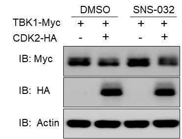
References:
(1) Mechanism of action of SNS-032, a novel cyclin-dependent kinase inhibitor, in chronic lymphocytic leukemia. Blood. 2009 May 7;113(19):4637-45.
(2) SNS-032 is a potent and selective CDK 2, 7 and 9 inhibitor that drives target modulation in patient samples. Cancer Chemother Pharmacol. 2009 Sep;64(4):723-32.
intention ontologique,
Je ne comprend pas la formulation. Peut-être pourrait-on formuler les choses en disant qu'on part d'une conversion éthique à partir de laquelle un nouveau rapport à soi, à autrui et au monde se construit.
à l’intérieur de ce charisme
Je ne comprends pas la formulation. Le terme de charisme devrait être plus introduit, même s'il est par ailleurs commun en management.
d’une praxis du leader et des subordonnés
Qualifier une telle praxis ainsi, n'est-ce pas d'emblée la figer dans un rapport pratico-inerte?
Chicago and Lasalle, Illinois, Open Court Publishing.
Respecter la même norme de citation pour toutes les références
renvoie l’être au monde sans essence.
formulation incorrecte: "il renvoie à l'être au monde sans essence"? Ne s'agit-il pas plutôt de la liberté, dont Sartre dit qu'elle n'a pas d'essence.
Anthropologie de la morale et de l'éthique
Titre à souligner
Sartre, J. P. (1976). L’être et le néant (1943). Gallimard, coll.«Tel» Sartre, J. P. (1992). L’existentialisme est un humanisme (1945). Folio. Sartre, J. P. (1960). Critique de la raison dialectique. Gallimard.
Les citations seront à normaliser. Si l'on suit la norme APA 7, l'éditeur Gallimard suffit, me semble-t-il
On expurge, on vide, on supprime toutes choses ou êtres dont notre conscience n’a pas besoin et qui ne sont pas prépondérants à notre existence.
J'ai du mal à comprendre la formule. De plus elle ne correspond pas au sens sartrien de la néantisation. le passage semble reprendre des analyses de l'absence. Elles se situe au niveau de la perception et vise une interprétation dynamique du phénomène forme/fond
Sartre, 1943
Le terme est absent à ma connaissance en 1943. La référence à la critique de la raison dialectique suffit.
l’énigmatique pour-soi-en-soi.
Ce point ne serait-il pas à éclaircir? Vise-t-on le pour-soi devenu en-soi comme passé ou le pour-soi-en-soi comme antivaleur? Il semble que l'analyse fasse référence à la reprise sartrienne de l'angoisse et à l'effondrement des déterminisme et engagement antérieurs face à vertige du dilemme actuel.
et même libre de ne pas exercer cette liberté
La formule sartrienne "nous sommes condamnés à la liberté" semble dire l'inverse. Il s'agit plutôt de fuir notre liberté dans la mauvaise foi, ce que nous faisons librement.
ontroverse de l’œuvre
de la controverse sur l'oeuvre
La figure suivante
La figure n'a pu être consultée.
d’être soi-même et pour soi-même
erreur dans la citation. Citation correcte: "d'être à soi-même et pour soi-même" (p. 490)
La conversion peut se révéler
La conversion ne peut se révéler
L’authenticité
Une question importante et qui n'est pas abordée est celle du lien entre la notion sartrienne d'authenticité et son acceptation actuelle dans l'étude du leadership. Il n'est pas sûr que les deux notions se recouvrent. La question devrait être posée si certaines manières de comprendre l'authenticité ne relèvent pas en fait de la mauvaise foi.
Note: This preprint has been reviewed by subject experts for Review Commons. Content has not been altered except for formatting.
Learn more at Review Commons
The study has carefully controlled and rigorous data. For the most part, the results are consistent with their claims. Except for a few modifications, it should be published. My suggestions are:
This manuscript describes an interesting study of developmental robustness and its intersection with organismal metabolism. It builds upon prior papers that have addressed the link between metabolism and development. It describes an ingenious approach to the problem and uncovers maltose metabolism in Drosophila as one such connection to sensory organ development and patterning. The important take home message for me is that they found natural genetic variants from the wild that confer greater robustness to the fly's morphological development, and these genetic variants are found in an enzyme that broadly metabolizes maltose, a simple sugar. Whereas previous studies used genetic manipulation to impact metabolism, this study shows that genetic variants in the wild exhibit effects on robustness. It suggests there might be a tradeoff between more vigorous carbohydrate metabolism and fidelity in morphological development.
Note: This preprint has been reviewed by subject experts for Review Commons. Content has not been altered except for formatting.
Learn more at Review Commons
Summary:
In this study, the authors performed GWAS to identify associations between the mean bristle number in Drosophila melanogaster adults and different SNPs present in 95 lines of the DGRP panel rear at 18C. They selected genes harboring those SNPs linked to bristle number that also had a moderate or high expression at the third insta larva stage to perform an RNAi screen. This RNAi screen, which included 43 genes, identified Maltase-A1 (Mal-A1) as a contributor to bristle number. Therefore, the authors then focus on investigating possible metabolic and transcriptional changes underlying the effect of Mal-A1 knockdown on bristle number. After whole-body knockdown using the da-gal4 driver, the authors identified decreased glucose in whole body and hemolymph, and decreased dilp3 mRNA expression in whole body, intestine, and insulin producing cells (IPC) in the larva brain. Similar to a whole-body Mal-A1 knockdown, a gut epithelial cell-specific gal4 driver (NP1) also decreased dilp3 mRNA expression in the whole body and larva brain. The authors suggest that Mal-A1 activity in the intestine may affect bristle number through lowering available glucose in the intestine, which decreases circulating glucose levels in the hemolymph, and in turn decreases dilp3 mRNA expression in the larva brain, leading to decreased bristle number. Finally, to validate the influence of bristle number via dilp3-mediated insulin signaling in the brain, the authors reared larvae at 18C, which they showed increased bristle number. Supporting their proposed model, rearing larvae at 18C increased dilp3 mRNA expression in the brain, which correlated with increased bristle number.
Major comments:
Minor comments
While the significance of identifying a novel regulatory mechanism for developmental robustness in Drosophila melanogaster is high and would be interesting for a broad audience, the authors do not present convincing experimental evidence to support their hypothesis. This is due to the insufficient number of replicates as well as the lack of experiments showing a direct role of insulin signaling.
RRID:AB_2827374
DOI: 10.1101/2025.10.17.683101
Resource: (Cell Signaling Technology Cat# 55506, RRID:AB_2827374)
Curator: @scibot
SciCrunch record: RRID:AB_2827374
AWS is 10x slower than a dedicated server for the same price
The discussion was split between criticizing the video's methodology and debating the fundamental value proposition of hyperscale cloud providers versus traditional hosting.
Par conséquent, je mets la notion d’édition critique numérique du théâtre au centre de ma réflexion. En partant de l’étude approfondie de l’histoire de l’édition dramatique dans l’environnement numérique, je considère reprendre le paradigme de l’édition traditionnelle et je veux proposer une nouvelle manière d’éditer qui nous permet de rester dans le sillage de la tradition tout en produisant, avec le même outil, une version numérique augmentée et complémentaire. Robert Alessi (Alessi, 2020) a développé cette dynamique en particulier à travers son outil ekdosis et l’a appliquée notamment aux textes classiques. Bien qu’il existe des applications au théâtre, elles se font au sein de la littérature fragmentaire latine (Debouy, 2021) ; par conséquent, cet outil s’avère incomplet pour l’édition du théâtre classique.
Conclusion très claire
avec l’édition critique
je rappellerais : "la mise en relation entre édition numérique et édition critique"
(Vitali-Rosati et Eberle Sinatra, 2014)
à placer après la citation ?
la couple
l'association entre "édition" et "numérique" ?
Matriz de experimentos
tra la la la
These items ask about different skills, from text editing in digital services to identifying the source of an error in software.
Deberíamos identificar en este párrafo la diferencia entre PISA e ICILS en considerar las nuevas dimensiones del DIig Comp...
Despite distinct approach, the two studies contain tasks that can be categorized into a more general dimension and a specialized one. PISA and ICILS share items that focus on tasks with a low degree of technical complexity, such as searching for information online and/or editing text for a school subject, but both studies also include items that refer to the creation and maintenance of web pages or programming software.
esto no debería enfatizar que es posible hacer la distinción en PISA? (en ICILS viene por diseño)
Digital self-efficacy
este párrafo es el central, y no está lo suficientemente enfatizado, parece que fuera una información adicional, y no se entiende la relación de la bidimensionalidad con la primera oración.
Studies focusing on capabilities usually emphasize the magnitude of the task, i.e., its degree of difficulty or complexity, and the linear achievement of the masterization process. By contrast, studies focused on attitudinal
no queda clara la conexión con lo anterior: task are capabilities?
Digital Self-efficacy
pero esto no es lo que ya aparecía arriba? o sea, no queda claro si lo de Ulfert-Blank es otro tipo de DSE?
Note: This response was posted by the corresponding author to Review Commons. The content has not been altered except for formatting.
Learn more at Review Commons
Reviewer #1 (Evidence, reproducibility and clarity (Required)):
These authors have developed a method to induce MI or MII arrest. While this was previously possible in MI, the advantage of the method presented here is it works for MII, and chemically inducible because it is based on a system that is sensitive to the addition of ABA. Depending on when the ABA is added, they achieve a MI or MII delay. The ABA promotes dimerizing fragments of Mps1 and Spc105 that can't bind their chromosomal sites. The evidence that the MI arrest is weaker than the MII arrest is convincing and consistent with published data and indicating the SAC in MI is less robust than MII or mitosis. The authors use this system to find evidence that the weak MI arrest is associated with PP1 binding to Spc105. This is a nice use of the system.
The remainder of the paper uses the SynSAC system to isolate populations enriched for MI or MII stages and conduct proteomics. This shows a powerful use of the system but more work is needed to validate these results, particularly in normal cells.
Overall the most significant aspect of this paper is the technical achievement, which is validated by the other experiments. They have developed a system and generated some proteomics data that maybe useful to others when analyzing kinetochore composition at each division. Overall, I have only a few minor suggestions.
We appreciate the reviewers’ support of our study.
1) In wild-type - Pds1 levels are high during M1 and A1, but low in MII. Can the authors comment on this? In line 217, what is meant by "slightly attenuated? Can the authors comment on how anaphase occurs in presence of high Pds1? There is even a low but significant level in MII.
The higher levels of Pds1 in meiosis I compared to meiosis II has been observed previously using immunofluorescence and live imaging1–3. Although the reasons are not completely clear, we speculate that there is insufficient time between the two divisions to re-accumulate Pds1 prior to separase re-activation.
We agree “slightly attenuated” was confusing and we have re-worded this sentence to read “Addition ABA at the time of prophase release resulted in Pds1securin stabilisation throughout the time course, consistent with delays in both metaphase I and II”.
We do not believe that either anaphase I or II occur in the presence of high Pds1. Western blotting represents the amount of Pds1 in the population of cells at a given time point. The time between meiosis I and II is very short even when treated with ABA. For example, in Figure 2B, spindle morphology counts show that the anaphase I peak is around 40% at its maxima (105 min) and around 40% of cells are in either metaphase I or metaphase II, and will be Pds1 positive. In contrast, due to the better efficiency of meiosis II, anaphase II hardly occurs at all in these conditions, since anaphase II spindles (and the second nuclear division) are observed at very low frequency (maximum 10%) from 165 minutes onwards. Instead, metaphase II spindles partially or fully breakdown, without undergoing anaphase extension. Taking Pds1 levels from the western blot and the spindle data together leads to the conclusion that at the end of the time-course, these cells are biochemically in metaphase II, but unable to maintain a robust spindle. Spindle collapse is also observed in other situations where meiotic exit fails, and potentially reflects an uncoupling of the cell cycle from the programme governing gamete differentiation3–5. We will explain this point in a revised version while referring to representative images that from evidence for this, as also requested by the reviewer below.
2) The figures with data characterizing the system are mostly graphs showing time course of MI and MII. There is no cytology, which is a little surprising since the stage is determined by spindle morphology. It would help to see sample sizes (ie. In the Figure legends) and also representative images. It would also be nice to see images comparing the same stage in the SynSAC cells versus normal cells. Are there any differences in the morphology of the spindles or chromosomes when in the SynSAC system?
This is an excellent suggestion and will also help clarify the point above. We will provide images of cells at the different stages. For each timepoint, 100 cells were scored. We have already included this information in the figure legends
3) A possible criticism of this system could be that the SAC signal promoting arrest is not coming from the kinetochore. Are there any possible consequences of this? In vertebrate cells, the RZZ complex streams off the kinetochore. Yeast don't have RZZ but this is an example of something that is SAC dependent and happens at the kinetochore. Can the authors discuss possible limitations such as this? Does the inhibition of the APC effect the native kinetochores? This could be good or bad. A bad possibility is that the cell is behaving as if it is in MII, but the kinetochores have made their microtubule attachments and behave as if in anaphase.
In our view, the fact that SynSAC does not come from kinetochores is a major advantage as this allows the study of the kinetochore in an unperturbed state. It is also important to note that the canonical checkpoint components are all still present in the SynSAC strains, and perturbations in kinetochore-microtubule interactions would be expected to mount a kinetochore-driven checkpoint response as normal. Indeed, it would be interesting in future work to understand how disrupting kinetochore-microtubule attachments alters kinetochore composition (presumably checkpoint proteins will be recruited) and phosphorylation but this is beyond the scope of this work. In terms of the state at which we are arresting cells – this is a true metaphase because cohesion has not been lost but kinetochore-microtubule attachments have been established. This is evident from the enrichment of microtubule regulators but not checkpoint proteins in the kinetochore purifications from metaphase I and II. While this state is expected to occur only transiently in yeast, since the establishment of proper kinetochore-microtubule attachments triggers anaphase onset, the ability to capture this properly bioriented state will be extremely informative for future studies. We appreciate the reviewers’ insight in highlighting these interesting discussion points which we will include in a revised version.
Reviewer #1 (Significance (Required)):
These authors have developed a method to induce MI or MII arrest. While this was previously possible in MI, the advantage of the method presented here is it works for MII, and chemically inducible because it is based on a system that is sensitive to the addition of ABA. Depending on when the ABA is added, they achieve a MI or MII delay. The ABA promotes dimerizing fragments of Mps1 and Spc105 that can't bind their chromosomal sites. The evidence that the MI arrest is weaker than the MII arrest is convincing and consistent with published data and indicating the SAC in MI is less robust than MII or mitosis. The authors use this system to find evidence that the weak MI arrest is associated with PP1 binding to Spc105. This is a nice use of the system.
The remainder of the paper uses the SynSAC system to isolate populations enriched for MI or MII stages and conduct proteomics. This shows a powerful use of the system but more work is needed to validate these results, particularly in normal cells.
Overall the most significant aspect of this paper is the technical achievement, which is validated by the other experiments. They have developed a system and generated some proteomics data that maybe useful to others when analyzing kinetochore composition at each division.
We appreciate the reviewer’s enthusiasm for our work.
Reviewer #2 (Evidence, reproducibility and clarity (Required)):
The manuscript submitted by Koch et al. describes a novel approach to collect budding yeast cells in metaphase I or metaphase II by synthetically activating the spinde checkpoint (SAC). The arrest is transient and reversible. This synchronization strategy will be extremely useful for studying meiosis I and meiosis II, and compare the two divisions. The authors characterized this so-named syncSACapproach and could confirm previous observations that the SAC arrest is less efficient in meiosis I than in meiosis II. They found that downregulation of the SAC response through PP1 phosphatase is stronger in meiosis I than in meiosis II. The authors then went on to purify kinetochore-associated proteins from metaphase I and II extracts for proteome and phosphoproteome analysis. Their data will be of significant interest to the cell cycle community (they compared their datasets also to kinetochores purified from cells arrested in prophase I and -with SynSAC in mitosis).
I have only a couple of minor comments:
1) I would add the Suppl Figure 1A to main Figure 1A. What is really exciting here is the arrest in metaphase II, so I don't understand why the authors characterize metaphase I in the main figure, but not metaphase II. But this is only a suggestion.
This is a good suggestion, we will do this in our full revision.
2) Line 197, the authors state: ...SyncSACinduced a more pronounced delay in metaphase II than in metaphase I. However, line 229 and 240 the auhtors talk about a "longer delay in metaphase Thank you for pointing this out, this is indeed a typo and we have corrected it.
3) The authors describe striking differences for both protein abundance and phosphorylation for key kinetochore associated proteins. I found one very interesting protein that seems to be very abundant and phosphorylated in metaphase I but not metaphase II, namely Sgo1. Do the authors think that Sgo1 is not required in metaphase II anymore? (Top hit in suppl Fig 8D).
This is indeed an interesting observation, which we plan to investigate as part of another study in the future. Indeed, data from mouse indicates that shugoshin-dependent cohesin deprotection is already absent in meiosis II in mouse oocytes6, though whether this is also true in yeast is not known. Furthermore, this does not rule out other functions of Sgo1 in meiosis II (for example promoting biorientation). We will include this point in the discussion.
Reviewer #2 (Significance (Required)):
The technique described here will be of great interest to the cell cycle community. Furthermore, the authors provide data sets on purified kinetochores of different meiotic stages and compare them to mitosis. This paper will thus be highly cited, for the technique, and also for the application of the technique.
Reviewer #3 (Evidence, reproducibility and clarity (Required)):
In their manuscript, Koch et al. describe a novel strategy to synchronize cells of the budding yeast Saccharomyces cerevisiae in metaphase I and metaphase II, thereby facilitating comparative analyses between these meiotic stages. This approach, termed SynSAC, adapts a method previously developed in fission yeast and human cells that enables the ectopic induction of a synthetic spindle assembly checkpoint (SAC) arrest by conditionally forcing the heterodimerization of two SAC components upon addition of the plant hormone abscisic acid (ABA). This is a valuable tool, which has the advantage that induces SAC-dependent inhibition of the anaphase promoting complex without perturbing kinetochores. Furthermore, since the same strategy and yeast strain can be also used to induce a metaphase arrest during mitosis, the methodology developed by Koch et al. enables comparative analyses between mitotic and meiotic cell divisions. To validate their strategy, the authors purified kinetochores from meiotic metaphase I and metaphase II, as well as from mitotic metaphase, and compared their protein composition and phosphorylation profiles. The results are presented clearly and in an organized manner.
We are grateful to the reviewer for their support.
Despite the relevance of both the methodology and the comparative analyses, several main issues should be addressed: 1.- In contrast to the strong metaphase arrest induced by ABA addition in mitosis (Supp. Fig. 2), the SynSAC strategy only promotes a delay in metaphase I and metaphase II as cells progress through meiosis. This delay extends the duration of both meiotic stages, but does not markedly increase the percentage of metaphase I or II cells in the population at a given timepoint of the meiotic time course (Fig. 1C). Therefore, although SynSAC broadens the time window for sample collection, it does not substantially improve differential analyses between stages compared with a standard NDT80 prophase block synchronization experiment. Could a higher ABA concentration or repeated hormone addition improve the tightness of the meiotic metaphase arrest?
For many purposes the enrichment and extended time for sample collection is sufficient, as we demonstrate here. However, as pointed out by the reviewer below, the system can be improved by use of the 4A-RASA mutations to provide a stronger arrest (see our response below). We did not experiment with higher ABA concentrations or repeated addition since the very robust arrest achieved with the 4A-RASA mutant deemed this unnecessary.
2.- Unlike the standard SynSAC strategy, introducing mutations that prevent PP1 binding to the SynSAC construct considerably extended the duration of the meiotic metaphase arrests. In particular, mutating PP1 binding sites in both the RVxF (RASA) and the SILK (4A) motifs of the Spc105(1-455)-PYL construct caused a strong metaphase I arrest that persisted until the end of the meiotic time course (Fig. 3A). This stronger and more prolonged 4A-RASA SynSAC arrest would directly address the issue raised above. It is unclear why the authors did not emphasize more this improved system. Indeed, the 4A-RASA SynSAC approach could be presented as the optimal strategy to induce a conditional metaphase arrest in budding yeast meiosis, since it not only adapts but also improves the original methods designed for fission yeast and human cells. Along the same lines, it is surprising that the authors did not exploit the stronger arrest achieved with the 4A-RASA mutant to compare kinetochore composition at meiotic metaphase I and II.
We agree that the 4A-RASA mutant is the best tool to use for the arrest and going forward this will be our approach. We collected the proteomics data and the data on the SynSAC mutant variants concurrently, so we did not know about the improved arrest at the time the proteomics experiment was done. Because very good arrest was already achieved with the unmutated SynSAC construct, we could not justify repeating the proteomics experiment which is a large amount of work using significant resources. However, we will highlight the potential of the 4A-RASA mutant more prominently in our full revision.
3.- The results shown in Supp. Fig. 4C are intriguing and merit further discussion. Mitotic growth in ABA suggest that the RASA mutation silences the SynSAC effect, yet this was not observed for the 4A or the double 4A-RASA mutants. Notably, in contrast to mitosis, the SynSAC 4A-RASA mutation leads to a more pronounced metaphase I meiotic delay (Fig. 3A). It is also noteworthy that the RVAF mutation partially restores mitotic growth in ABA. This observation supports, as previously demonstrated in human cells, that Aurora B-mediated phosphorylation of S77 within the RVSF motif is important to prevent PP1 binding to Spc105 in budding yeast as well.
We agree these are intriguing findings that highlight key differences as to the wiring of the spindle checkpoint in meiosis and mitosis and potential for future studies, however, currently we can only speculate as to the underlying cause. The effect of the RASA mutation in mitosis is unexpected and unexplained. However, the fact that the 4A-RASA mutation causes a stronger delay in meiosis I compared to mitosis can be explained by a greater prominence of PP1 phosphatase in meiosis. Indeed, our data (Figure 4A) show that the PP1 phosphatase Glc7 and its regulatory subunit Fin1 are highly enriched on kinetochores at all meiotic stages compared to mitosis.
We agree that the improved growth of the RVAF mutant is intriguing and points to a role of Aurora B-mediated phosphorylation, though previous work has not supported such a role 7.
We will include a discussion of these important points in a revised version.
4.- To demonstrate the applicability of the SynSAC approach, the authors immunoprecipitated the kinetochore protein Dsn1 from cells arrested at different meiotic or mitotic stages, and compared kinetochore composition using data independent acquisition (DIA) mass spectrometry. Quantification and comparative analyses of total and kinetochore protein levels were conducted in parallel for cells expressing either FLAG-tagged or untagged Dsn1 (Supp. Fig. 7A-B). To better detect potential changes, protein abundances were next scaled to Dsn1 levels in each sample (Supp. Fig. 7C-D). However, it is not clear why the authors did not normalize protein abundance in the immunoprecipitations from tagged samples at each stage to the corresponding untagged control, instead of performing a separate analysis. This would be particularly relevant given the high sensitivity of DIA mass spectrometry, which enabled quantification of thousands of proteins. Furthermore, the authors compared protein abundances in tagged-samples from mitotic metaphase and meiotic prophase, metaphase I and metaphase II (Supp. Fig. 7E-F). If protein amounts in each case were not normalized to the untagged controls, as inferred from the text (lines 333 to 338), the observed differences could simply reflect global changes in protein expression at different stages rather than specific differences in protein association to kinetochores.
While we agree with the reviewer that at first glance, normalising to no tag makes the most sense, in practice there is very low background signal in the no tag sample which means that any random fluctuations have a big impact on the final fold change. This approach therefore introduces artefacts into the data rather than improving normalisation.
To provide reassurance that our kinetochore immunoprecipitations are specific, and that the background (no tag) signal is indeed very low, we will provide a new supplemental figure showing the volcanos comparing kinetochore purifications at each stage with their corresponding no tag control. These volcano plots show very clearly that the major enriched proteins are kinetochore proteins and associated factors, in all cases.
It is also important to note that our experiment looks at relative changes of the same protein over time, which we expect to be relatively small in the whole cell lysate. We previously documented proteins that change in abundance in whole cell lysates throughout meiosis8. In this study, we found that relatively few proteins significantly change in abundance, supporting this view.
Our aim in the current study was to understand how the relative composition of the kinetochore changes and for this, we believe that a direct comparison to Dsn1, a central kinetochore protein which we immunoprecipitated is the most appropriate normalisation.
5.- Despite the large amount of potentially valuable data generated, the manuscript focuses mainly on results that reinforce previously established observations (e.g., premature SAC silencing in meiosis I by PP1, changes in kinetochore composition, etc.). The discussion would benefit from a deeper analysis of novel findings that underscore the broader significance of this study.
We strongly agree with this point and we will re-frame the discussion to focus on the novel findings, as also raised by the other reviewers.
Finally, minor concerns are: 1.- Meiotic progression in SynSAC strains lacking Mad1, Mad2 or Mad3 is severely affected (Fig. 1D and Supp. Fig. 1), making it difficult to assess whether, as the authors state, the metaphase delays depend on the canonical SAC cascade. In addition, as a general note, graphs displaying meiotic time courses could be improved for clarity (e.g., thinner data lines, addition of axis gridlines and external tick marks, etc.).
We will generate the data to include a checkpoint mutant +/- ABA for direct comparison. We will take steps to improve the clarity of presentation of the meiotic timecourse graphs, though our experience is that uncluttered graphs make it easier to compare trends.
2.- Spore viability following SynSAC induction in meiosis was used as an indicator that this experimental approach does not disrupt kinetochore function and chromosome segregation. However, this is an indirect measure. Direct monitoring of genome distribution using GFP-tagged chromosomes would have provided more robust evidence. Notably, the SynSAC mad3Δ mutant shows a slight viability defect, which might reflect chromosome segregation defects that are more pronounced in the absence of a functional SAC.
Spore viability is a much more sensitive way of analysing segregation defects that GFP-labelled chromosomes. This is because GFP labelling allows only a single chromosome to be followed. On the other hand, if any of the 16 chromosomes mis-segregate in a given meiosis this would result in one or more aneuploid spores in the tetrad, which are typically inviable. The fact that spore viability is not significantly different from wild type in this analysis indicates that there are no major chromosome segregation defects in these strains, and we therefore do not plan to do this experiment.
3.- It is surprising that, although SAC activity is proposed to be weaker in metaphase I, the levels of CPC/SAC proteins seem to be higher at this stage of meiosis than in metaphase II or mitotic metaphase (Fig. 4A-B).
We agree, this is surprising and we will point this out in the revised discussion. We speculate that the challenge in biorienting homologs which are held together by chiasmata, rather than back-to-back kinetochores results in a greater requirement for error correction in meiosis I. Interestingly, the data with the RASA mutant also point to increased PP1 activity in meiosis I, and we additionally observed increased levels of PP1 (Glc7 and Fin1) on meiotic kinetochores, consistent with the idea that cycles of error correction and silencing are elevated in meiosis I.
4.- Although a more detailed exploration of kinetochore composition or phosphorylation changes is beyond the scope of the manuscript, some key observations could have been validated experimentally (e.g., enrichment of proteins at kinetochores, phosphorylation events that were identified as specific or enriched at a certain meiotic stage, etc.).
We agree that this is beyond the scope of the current study but will form the start of future projects from our group, and hopefully others.
5.- Several typographical errors should be corrected (e.g., "Knetochores" in Fig. 4 legend, "250uM ABA" in Supp. Fig. 1 legend, etc.)
Thank you for pointing these out, they have been corrected.
Reviewer #3 (Significance (Required)):
Koch et al. describe a novel methodology, SynSAC, to synchronize budding yeast cells in metaphase I or metaphase II during meiosis, as well and in mitotic metaphase, thereby enabling differential analyses among these cell division stages. Their approach builds on prior strategies originally developed in fission yeast and human cells models to induce a synthetic spindle assembly checkpoint (SAC) arrest by conditionally forcing the heterodimerization of two SAC proteins upon addition of abscisic acid (ABA). The results from this manuscript are of special relevance for researchers studying meiosis and using Saccharomyces cerevisiae as a model. Moreover, the differential analysis of the composition and phosphorylation of kinetochores from meiotic metaphase I and metaphase II adds interest for the broader meiosis research community. Finally, regarding my expertise, I am a researcher specialized in the regulation of cell division.
Note: This preprint has been reviewed by subject experts for Review Commons. Content has not been altered except for formatting.
Learn more at Review Commons
In their manuscript, Koch et al. describe a novel strategy to synchronize cells of the budding yeast Saccharomyces cerevisiae in metaphase I and metaphase II, thereby facilitating comparative analyses between these meiotic stages. This approach, termed SynSAC, adapts a method previously developed in fission yeast and human cells that enables the ectopic induction of a synthetic spindle assembly checkpoint (SAC) arrest by conditionally forcing the heterodimerization of two SAC components upon addition of the plant hormone abscisic acid (ABA). This is a valuable tool, which has the advantage that induces SAC-dependent inhibition of the anaphase promoting complex without perturbing kinetochores. Furthermore, since the same strategy and yeast strain can be also used to induce a metaphase arrest during mitosis, the methodology developed by Koch et al. enables comparative analyses between mitotic and meiotic cell divisions. To validate their strategy, the authors purified kinetochores from meiotic metaphase I and metaphase II, as well as from mitotic metaphase, and compared their protein composition and phosphorylation profiles. The results are presented clearly and in an organized manner. Despite the relevance of both the methodology and the comparative analyses, several main issues should be addressed:
1.- In contrast to the strong metaphase arrest induced by ABA addition in mitosis (Supp. Fig. 2), the SynSAC strategy only promotes a delay in metaphase I and metaphase II as cells progress through meiosis. This delay extends the duration of both meiotic stages, but does not markedly increase the percentage of metaphase I or II cells in the population at a given timepoint of the meiotic time course (Fig. 1C). Therefore, although SynSAC broadens the time window for sample collection, it does not substantially improve differential analyses between stages compared with a standard NDT80 prophase block synchronization experiment. Could a higher ABA concentration or repeated hormone addition improve the tightness of the meiotic metaphase arrest? 2.- Unlike the standard SynSAC strategy, introducing mutations that prevent PP1 binding to the SynSAC construct considerably extended the duration of the meiotic metaphase arrests. In particular, mutating PP1 binding sites in both the RVxF (RASA) and the SILK (4A) motifs of the Spc105(1-455)-PYL construct caused a strong metaphase I arrest that persisted until the end of the meiotic time course (Fig. 3A). This stronger and more prolonged 4A-RASA SynSAC arrest would directly address the issue raised above. It is unclear why the authors did not emphasize more this improved system. Indeed, the 4A-RASA SynSAC approach could be presented as the optimal strategy to induce a conditional metaphase arrest in budding yeast meiosis, since it not only adapts but also improves the original methods designed for fission yeast and human cells. Along the same lines, it is surprising that the authors did not exploit the stronger arrest achieved with the 4A-RASA mutant to compare kinetochore composition at meiotic metaphase I and II. 3.- The results shown in Supp. Fig. 4C are intriguing and merit further discussion. Mitotic growth in ABA suggest that the RASA mutation silences the SynSAC effect, yet this was not observed for the 4A or the double 4A-RASA mutants. Notably, in contrast to mitosis, the SynSAC 4A-RASA mutation leads to a more pronounced metaphase I meiotic delay (Fig. 3A). It is also noteworthy that the RVAF mutation partially restores mitotic growth in ABA. This observation supports, as previously demonstrated in human cells, that Aurora B-mediated phosphorylation of S77 within the RVSF motif is important to prevent PP1 binding to Spc105 in budding yeast as well. 4.- To demonstrate the applicability of the SynSAC approach, the authors immunoprecipitated the kinetochore protein Dsn1 from cells arrested at different meiotic or mitotic stages, and compared kinetochore composition using data independent acquisition (DIA) mass spectrometry. Quantification and comparative analyses of total and kinetochore protein levels were conducted in parallel for cells expressing either FLAG-tagged or untagged Dsn1 (Supp. Fig. 7A-B). To better detect potential changes, protein abundances were next scaled to Dsn1 levels in each sample (Supp. Fig. 7C-D). However, it is not clear why the authors did not normalize protein abundance in the immunoprecipitations from tagged samples at each stage to the corresponding untagged control, instead of performing a separate analysis. This would be particularly relevant given the high sensitivity of DIA mass spectrometry, which enabled quantification of thousands of proteins. Furthermore, the authors compared protein abundances in tagged-samples from mitotic metaphase and meiotic prophase, metaphase I and metaphase II (Supp. Fig. 7E-F). If protein amounts in each case were not normalized to the untagged controls, as inferred from the text (lines 333 to 338), the observed differences could simply reflect global changes in protein expression at different stages rather than specific differences in protein association to kinetochores. 5.- Despite the large amount of potentially valuable data generated, the manuscript focuses mainly on results that reinforce previously established observations (e.g., premature SAC silencing in meiosis I by PP1, changes in kinetochore composition, etc.). The discussion would benefit from a deeper analysis of novel findings that underscore the broader significance of this study.
Finally, minor concerns are:
1.- Meiotic progression in SynSAC strains lacking Mad1, Mad2 or Mad3 is severely affected (Fig. 1D and Supp. Fig. 1), making it difficult to assess whether, as the authors state, the metaphase delays depend on the canonical SAC cascade. In addition, as a general note, graphs displaying meiotic time courses could be improved for clarity (e.g., thinner data lines, addition of axis gridlines and external tick marks, etc.). 2.- Spore viability following SynSAC induction in meiosis was used as an indicator that this experimental approach does not disrupt kinetochore function and chromosome segregation. However, this is an indirect measure. Direct monitoring of genome distribution using GFP-tagged chromosomes would have provided more robust evidence. Notably, the SynSAC mad3Δ mutant shows a slight viability defect, which might reflect chromosome segregation defects that are more pronounced in the absence of a functional SAC. 3.- It is surprising that, although SAC activity is proposed to be weaker in metaphase I, the levels of CPC/SAC proteins seem to be higher at this stage of meiosis than in metaphase II or mitotic metaphase (Fig. 4A-B). 4.- Although a more detailed exploration of kinetochore composition or phosphorylation changes is beyond the scope of the manuscript, some key observations could have been validated experimentally (e.g., enrichment of proteins at kinetochores, phosphorylation events that were identified as specific or enriched at a certain meiotic stage, etc.). 5.- Several typographical errors should be corrected (e.g., "Knetochores" in Fig. 4 legend, "250uM ABA" in Supp. Fig. 1 legend, etc.)
Koch et al. describe a novel methodology, SynSAC, to synchronize budding yeast cells in metaphase I or metaphase II during meiosis, as well and in mitotic metaphase, thereby enabling differential analyses among these cell division stages. Their approach builds on prior strategies originally developed in fission yeast and human cells models to induce a synthetic spindle assembly checkpoint (SAC) arrest by conditionally forcing the heterodimerization of two SAC proteins upon addition of abscisic acid (ABA). The results from this manuscript are of special relevance for researchers studying meiosis and using Saccharomyces cerevisiae as a model. Moreover, the differential analysis of the composition and phosphorylation of kinetochores from meiotic metaphase I and metaphase II adds interest for the broader meiosis research community. Finally, regarding my expertise, I am a researcher specialized in the regulation of cell division.
Note: This preprint has been reviewed by subject experts for Review Commons. Content has not been altered except for formatting.
Learn more at Review Commons
The manuscript submitted by Koch et al. describes a novel approach to collect budding yeast cells in metaphase I or metaphase II by synthetically activating the spinde checkpoint (SAC). The arrest is transient and reversible. This synchronization strategy will be extremely useful for studying meiosis I and meiosis II, and compare the two divisions. The authors characterized this so-named syncSACapproach and could confirm previous observations that the SAC arrest is less efficient in meiosis I than in meiosis II. They found that downregulation of the SAC response through PP1 phosphatase is stronger in meiosis I than in meiosis II. The authors then went on to purify kinetochore-associated proteins from metaphase I and II extracts for proteome and phosphoproteome analysis. Their data will be of significant interest to the cell cycle community (they compared their datasets also to kinetochores purified from cells arrested in prophase I and -with SynSAC in mitosis).
I have only a couple of minor comments:
1) I would add the Suppl Figure 1A to main Figure 1A. What is really exciting here is the arrest in metaphase II, so I don't understand why the authors characterize metaphase I in the main figure, but not metaphase II. But this is only a suggestion.
2) Line 197, the authors state: ...SyncSACinduced a more pronounced delay in metaphase II than in metaphase I. However, line 229 and 240 the auhtors talk about a "longer delay in metaphase <i compared to metaphase II"... this seems to be a mix-up.
3) The authors describe striking differences for both protein abundance and phosphorylation for key kinetochore associated proteins. I found one very interesting protein that seems to be very abundant and phosphorylated in metaphase I but not metaphase II, namely Sgo1. Do the authors think that Sgo1 is not required in metaphase II anymore? (Top hit in suppl Fig 8D).
The technique described here will be of great interest to the cell cycle community. Furthermore, the authors provide data sets on purified kinetochores of different meiotic stages and compare them to mitosis. This paper will thus be highly cited, for the technique, and also for the application of the technique.
Author response:
The following is the authors’ response to the original reviews.
Reviewer #1 (Public review):
Summary
This work performed Raman spectral microscopy at the single-cell level for 15 different culture conditions in E. coli. The Raman signature is systematically analyzed and compared with the proteome dataset of the same culture conditions. With a linear model, the authors revealed correspondence between Raman pattern and proteome expression stoichiometry indicating that spectrometry could be used for inferring proteome composition in the future. With both Raman spectra and proteome datasets, the authors categorized co-expressed genes and illustrated how proteome stoichiometry is regulated among different culture conditions. Co-expressed gene clusters were investigated and identified as homeostasis core, carbon-source dependent, and stationary phase-dependent genes. Overall, the authors demonstrate a strong and solid data analysis scheme for the joint analysis of Raman and proteome datasets.
Strengths and major contributions
(1) Experimentally, the authors contributed Raman datasets of E. coli with various growth conditions.
(2) In data analysis, the authors developed a scheme to compare proteome and Raman datasets. Protein co-expression clusters were identified, and their biological meaning was investigated.
Weaknesses
The experimental measurements of Raman microscopy were conducted at the single-cell level; however, the analysis was performed by averaging across the cells. The author did not discuss if Raman microscopy can used to detect cell-to-cell variability under the same condition.
We thank the reviewer for raising this important point. Though this topic is beyond the scope of our study, some of our authors have addressed the application of single-cell Raman spectroscopy to characterizing phenotypic heterogeneity in individual Staphylococcus aureus cells in another paper (Kamei et al., bioRxiv, doi: 10.1101/2024.05.12.593718). Additionally, one of our authors demonstrated that single-cell RNA sequencing profiles can be inferred from Raman images of mouse cells (Kobayashi-Kirschvink et al., Nat. Biotechnol. 42, 1726–1734, 2024). Therefore, detecting cell-to-cell variability under the same conditions has been shown to be feasible. Whether averaging single-cell Raman spectra is necessary depends on the type of analysis and the available dataset. We will discuss this in more detail in our response to Comment (1) by Reviewer #1 (Recommendation for the authors).
Discussion and impact on the field
Raman signature contains both proteomic and metabolomic information and is an orthogonal method to infer the composition of biomolecules. It has the advantage that single-cell level data could be acquired and both in vivo and in vitro data can be compared. This work is a strong initiative for introducing the powerful technique to systems biology and providing a rigorous pipeline for future data analysis.
Reviewer #2 (Public review):
Summary and strengths:
Kamei et al. observe the Raman spectra of a population of single E. coli cells in diverse growth conditions. Using LDA, Raman spectra for the different growth conditions are separated. Using previously available protein abundance data for these conditions, a linear mapping from Raman spectra in LDA space to protein abundance is derived. Notably, this linear map is condition-independent and is consequently shown to be predictive for held-out growth conditions. This is a significant result and in my understanding extends the earlier Raman to RNA connection that has been reported earlier.
They further show that this linear map reveals something akin to bacterial growth laws (ala Scott/Hwa) that the certain collection of proteins shows stoichiometric conservation, i.e. the group (called SCG - stoichiometrically conserved group) maintains their stoichiometry across conditions while the overall scale depends on the conditions. Analyzing the changes in protein mass and Raman spectra under these conditions, the abundance ratios of information processing proteins (one of the large groups where many proteins belong to "information and storage" - ISP that is also identified as a cluster of orthologous proteins) remain constant. The mass of these proteins deemed, the homeostatic core, increases linearly with growth rate. Other SCGs and other proteins are condition-specific.
Notably, beyond the ISP COG the other SCGs were identified directly using the proteome data. Taking the analysis beyond they then how the centrality of a protein - roughly measured as how many proteins it is stoichiometric with - relates to function and evolutionary conservation. Again significant results, but I am not sure if these ideas have been reported earlier, for example from the community that built protein-protein interaction maps.
As pointed out, past studies have revealed that the function, essentiality, and evolutionary conservation of genes are linked to the topology of gene networks, including protein-protein interaction networks. However, to the best of our knowledge, their linkage to stoichiometry conservation centrality of each gene has not yet been established.
Previously analyzed networks, such as protein-protein interaction networks, depend on known interactions. Therefore, as our understanding of the molecular interactions evolves with new findings, the conclusions may change. Furthermore, analysis of a particular interaction network cannot account for effects from different types of interactions or multilayered regulations affecting each protein species.
In contrast, the stoichiometry conservation network in this study focuses solely on expression patterns as the net result of interactions and regulations among all types of molecules in cells. Consequently, the stoichiometry conservation networks are not affected by the detailed knowledge of molecular interactions and naturally reflect the global effects of multilayered interactions. Additionally, stoichiometry conservation networks can easily be obtained for non-model organisms, for which detailed molecular interaction information is usually unavailable. Therefore, analysis with the stoichiometry conservation network has several advantages over existing methods from both biological and technical perspectives.
We added a paragraph explaining this important point to the Discussion section, along with additional literature.
Finally, the paper built a lot of "machinery" to connect ¥Omega_LE, built directly from proteome, and ¥Omega_B, built from Raman, spaces. I am unsure how that helps and have not been able to digest the 50 or so pages devoted to this.
The mathematical analyses in the supplementary materials form the basis of the argument in the main text. Without the rigorous mathematical discussions, Fig. 6E — one of the main conclusions of this study — and Fig. 7 could never be obtained. Therefore, we believe the analyses are essential to this study. However, we clarified why each analysis is necessary and significant in the corresponding sections of the Results to improve the manuscript's readability.
Please see our responses to comments (2) and (7) by Reviewer #1 (Recommendations for the authors) and comments (5) and (6) by Reviewer #2 (Recommendations for the authors).
Strengths:
The rigorous analysis of the data is the real strength of the paper. Alongside this, the discovery of SCGs that are condition-independent and that are condition-dependent provides a great framework.
Weaknesses:
Overall, I think it is an exciting advance but some work is needed to present the work in a more accessible way.
We edited the main text to make it more accessible to a broader audience. Please see our responses to comments (2) and (7) by Reviewer #1 (Recommendations for the authors) and comments (5) and (6) by Reviewer #2 (Recommendations for the authors).
Reviewer #1 (Recommendations for the authors):
(1) The Raman spectral data is measured from single-cell imaging. In the current work, most of the conclusions are from averaged data. From my understanding, once the correspondence between LDA and proteome data is established (i.e. the matrix B) one could infer the single-cell proteome composition from B. This would provide valuable information on how proteome composition fluctuates at the single-cell level.
We can calculate single-cell proteomes from single-cell Raman spectra in the manner suggested by the reviewer. However, we cannot evaluate the accuracy of their estimation without single-cell proteome data under the same environmental conditions. Likewise, we cannot verify variations of estimated proteomes of single cells. Since quantitatively accurate single-cell proteome data is unavailable, we concluded that addressing this issue was beyond the scope of this study.
Nevertheless, we agree with the reviewer that investigating how proteome composition fluctuates at the single-cell level based on single-cell Raman spectra is an intriguing direction for future research. In this regard, some of our authors have studied the phenotypic heterogeneity of Staphylococcus aureus cells using single-cell Raman spectra in another paper (Kamei et al., bioRxiv, doi: 10.1101/2024.05.12.593718), and one of our authors has demonstrated that single-cell RNA sequencing profiles can be inferred from Raman images of mouse cells (Kobayashi-Kirschvink et al., Nat. Biotechnol. 42, 1726–1734, 2024). Therefore, it is highly plausible that single-cell Raman spectroscopy can also characterize proteomic fluctuations in single cells. We have added a paragraph to the Discussion section to highlight this important point.
(2) The establishment of matrix B is quite confusing for readers who only read the main text. I suggest adding a flow chart in Figure 1 to explain the data analysis pipeline, as well as state explicitly what is the dimension of B, LDA matrix, and proteome matrix.
We thank the reviewer for the suggestion. Following the reviewer's advice, we have explicitly stated the dimensions of the vectors and matrices in the main text. We have also added descriptions of the dimensions of the constructed spaces. Rather than adding another flow chart to Figure 1, we added a new table (Table 1) to explain the various symbols representing vectors and matrices, thereby improving the accessibility of the explanation.
(3) One of the main contributions for this work is to demonstrate how proteome stoichiometry is regulated across different conditions. A total of m=15 conditions were tested in this study, and this limits the rank of LDA matrix as 14. Therefore, maximally 14 "modes" of differential composition in a proteome can be detected.
As a general reader, I am wondering in the future if one increases or decreases the number of conditions (say m=5 or m=50) what information can be extracted? It is conceivable that increasing different conditions with distinct cellular physiology would be beneficial to "explore" different modes of regulation for cells. As proof of principle, I am wondering if the authors could test a lower number (by sub-sampling from m=15 conditions, e.g. picking five of the most distinct conditions) and see how this would affect the prediction of proteome stoichiometry inference.
We thank the reviewer for bringing an important point to our attention. To address the issue raised, we conducted a new subsampling analysis (Fig. S14).
As we described in the main text (Fig. 6E) and the supplementary materials, the m x m orthogonal matrix, Θ, represents to what extent the two spaces Ω<sub>LE</sub> and Ω<sub>B</sub> are similar (m is the number of conditions; in our main analysis, m = 15). Thus, the low-dimensional correspondence between the two spaces connected by an orthogonal transformation, such as an m-dimensional rotation, can be evaluated by examining the elements of the matrix Θ. Specifically, large off-diagonal elements of the matrix mix higher dimensions and lower dimensions, making the two spaces spanned by the first few major axes appear dissimilar. Based on this property, we evaluated the vulnerability of the low-dimensional correspondence between Ω<sub>LE</sub> and Ω<sub>B</sub> to the reduced number of conditions by measuring how close Θ was to the identity matrix when the analysis was performed on the subsampled datasets.
In the new figure (Fig. S14), we first created all possible smaller condition sets by subsampling the conditions. Next, to evaluate the closeness between the matrix Θ and the identity matrix for each smaller condition set, we generated 10,000 random orthogonal matrices of the same size as . We then evaluated the probability of obtaining a higher level of low-dimensional correspondence than that of the experimental data by chance (see section 1.8 of the Supplementary Materials). This analysis was already performed in the original manuscript for the non-subsampled case (m = 15) in Fig. S9C; the new analysis systematically evaluates the correspondence for the subsampled datasets.
The results clearly show that low-dimensional correspondence is more likely to be obtained with more conditions (Fig. S14). In particular, when the number of conditions used in the analysis exceeds five, the median of the probability that random orthogonal matrices were closer to the identity matrix than the matrix Θ calculated from subsampled experimental data became lower than 10<sup>-4</sup>. This analysis provides insight into the number of conditions required to find low-dimensional correspondence between Ω<sub>LE</sub> and Ω<sub>B</sub>.
What conditions are used in the analysis can change the low-dimensional structures of Ω<sub>LE</sub> and Ω<sub>B</sub> . Therefore, it is important to clarify whether including more conditions in the analysis reduces the dependence of the low-dimensional structures on conditions. We leave this issue as a subject for future study. This issue relates to the effective dimensionality of omics profiles needed to establish the diverse physiological states of cells across conditions. Determining the minimum number of conditions to attain the condition-independent low-dimensional structures of Ω<sub>LE</sub> and Ω<sub>B</sub> would provide insight into this fundamental problem. Furthermore, such an analysis would identify the range of applications of Raman spectra as a tool for capturing macroscopic properties of cells at the system level.
We now discuss this point in the Discussion section, referring to this analysis result (Fig. S14). Please also see our reply to the comment (1) by Reviewer #2 (Recommendations for the authors).
(4) In E. coli cells, total proteome is in mM concentration while the total metabolites are between 10 to 100 mM concentration. Since proteins are large molecules with more functional groups, they may contribute to more Raman signal (per molecules) than metabolites. Still, the meaningful quantity here is the "differential Raman signal" with different conditions, not the absolute signal. I am wondering how much percent of differential Raman signature are from proteome and how much are from metabolome.
It is an important and interesting question to what extent changes in the proteome and metabolome contribute to changes in Raman spectra. Though we concluded that answering this question is beyond the scope of this study, we believe it is an important topic for future research.
Raman spectral patterns convey the comprehensive molecular composition spanning the various omics layers of target cells. Changes in the composition of these layers can be highly correlated, and identifying their contributions to changes in Raman spectra would provide insight into the mutual correlation of different omics layers. Addressing the issue raised by the reviewer would expand the applications of Raman spectroscopy and highlight the advantage of cellular Raman spectra as a means of capturing comprehensive multi-omics information.
We note that some studies have evaluated the contributions of proteins, lipids, nucleic acids, and glycogen to the Raman spectra of mammalian cells and how these contributions change in different states (e.g., Mourant et al., J Biomed Opt, 10(3), 031106, 2005). Additionally, numerous studies have imaged or quantified metabolites in various cell types (see, for example, Cutshaw et al., Chemical Reviews, 123(13), 8297–8346, 2023, for a comprehensive review). Extending these approaches to multiple omics layers in future studies would help resolve the issue raised by the reviewer.
(5) It is known that E. coli cells in different conditions have different cell sizes, where cell width increases with carbon source quality and growth rate. Does this effect be normalized when processing the Raman signal?
Each spectrum was normalized by subtracting the average and dividing it by the standard deviation. This normalization minimizes the differences in signal intensities due to different cell sizes and densities. This information is shown in the Materials and Methods section of the Supplementary Materials.
(6) I have a question about interpretation of the centrality index. A higher centrality indicates the protein expression pattern is more aligned with the "mainstream" of the other proteins in the proteome. However, it is possible that the proteome has multiple" mainstream modes" (with possibly different contributions in magnitudes), and the centrality seems to only capture the "primary mode". A small group of proteins could all have low centrality but have very consistent patterns with high conservation of stoichiometry. I wondering if the author could discuss and clarify with this.
We thank the reviewer for drawing our attention to the insufficient explanation in the original manuscript. First, we note that stoichiometry conserving protein groups are not limited to those composed of proteins with high stoichiometry conservation centrality. The SCGs 2–5 are composed of proteins that strongly conserve stoichiometry within each group but have low stoichiometry conservation centrality (Fig. 5A, 5K, 5L, and 7A). In other words, our results demonstrate the existence of the "primary mainstream mode" (SCG 1, i.e., the homeostatic core) and condition-specific "non-primary mainstream modes" (SCGs 2–5). These primary and non-primary modes are distinguishable by their position along the axis of stoichiometry conservation centrality (Fig. 5A, 5K, and 5L).
However, a single one-dimensional axis (centrality) cannot capture all characteristics of stoichiometry-conserving architecture. In our case, the "non-primary mainstream modes" (SCGs 2–5) were distinguished from each other by multiple csLE axes.
To clarify this point, we modified the first paragraph of the section where we first introduce csLE (Revealing global stoichiometry conservation architecture of the proteomes with csLE). We also added a paragraph to the Discussion section regarding the condition-specific SCGs 2–5.
(7) Figures 3, 4, and 5A-I are analyses on proteome data and are not related to Raman spectral data. I am wondering if this part of the analysis can be re-organized and not disrupt the mainline of the manuscript.
We agree that the structure of this manuscript is complicated. Before submitting this manuscript to eLife, we seriously considered reorganizing it. However, we concluded that this structure was most appropriate because our focus on stoichiometry conservation cannot be explained without analyzing the coefficients of the Raman-proteome correspondence using COG classification (see Fig. 3; note that Fig. 3A relates to Raman data). This analysis led us to examine the global stoichiometry conservation architecture of proteomes (Figs. 4 and 5) and discover the unexpected similarity between the low-dimensional structures of Ω<sub>LE</sub> and Ω<sub>B</sub>
Therefore, we decided to keep the structure of the manuscript as it is. To partially resolve this issue, however, we added references to Fig. S1, the diagram of this paper’s mainline, to several places in the main text so that readers can more easily grasp the flow of the manuscript.
(8) Supplementary Equation (2.6) could be wrong. From my understanding of the coordinate transformation definition here, it should be [w1 ... ws] X := RHS terms in big parenthesis.
We checked the equation and confirmed that it is correct.
Reviewer #2 (Recommendations for the authors):
(1) The first main result or linear map between raman and proteome linked via B is intriguing in the sense that the map is condition-independent. A speculative question I have is if this relationship may become more complex or have more condition-dependent corrections as the number of conditions goes up. The 15 or so conditions are great but it is not clear if they are often quite restrictive. For example, they assume an abundance of most other nutrients. Now if you include a growth rate decrease due to nitrogen or other limitations, do you expect this to work?
In our previous paper (Kobayashi-Kirschvink et al., Cell Systems 7(1): 104–117.e4, 2018), we statistically demonstrated a linear correspondence between cellular Raman spectra and transcriptomes for fission yeast under 10 environmental conditions. These conditions included nutrient-rich and nutrient-limited conditions, such as nitrogen limitation. Since the Raman-transcriptome correspondence was only statistically verified in that study, we analyzed the data from the standpoint of stoichiometry conservation in this study. The results (Fig. S11 and S12) revealed a correspondence in lower dimensions similar to that observed in our main results. In addition, similar correspondences were obtained even for different E. coli strains under common culture conditions (Fig. S11 and S12). Therefore, it is plausible that the stoichiometry-conservation low-dimensional correspondence between Raman and gene expression profiles holds for a wide range of external and internal perturbations.
We agree with the reviewer that it is important to understand how Raman-omics correspondences change with the number of conditions. To address this issue, we examined how the correspondence between Ω<sub>LE</sub> and Ω<sub>B</sub> changes by subsampling the conditions used in the analysis. We focused on , which was introduced in Fig. 5E, because the closeness of Θ to the identity matrix represents correspondence precision. We found a general trend that the low-dimensional correspondence becomes more precise as the number of conditions increases (Fig. S14). This suggests that increasing the number of conditions generally improves the correspondence rather than disrupting it.
We added a paragraph to the Discussion section addressing this important point. Please also refer to our response to Comment (3) of Reviewer #1 (Recommendations for the authors).
(2) A little more explanation in the text for 3C/D would help. I am imagining 3D is the control for 3C. Minor comment - 3B looks identical to S4F but the y-axis label is different.
We thank the reviewer for pointing out the insufficient explanation of Fig. 3C and 3D in the main text. Following this advice, we added explanations of these plots to the main text. We also added labels ("ISP COG class" and "non-ISP COG class") to the top of these two figures.
Fig. 3B and S4F are different. For simplicity, we used the Pearson correlation coefficient in Fig. 3B. However, cosine similarity is a more appropriate measure for evaluating the degree of conservation of abundance ratios. Thus, we presented the result using cosine similarity in a supplementary figure (Fig. S4F). Please note that each point in Fig. S4F is calculated between proteome vectors of two conditions. The dimension of each proteome vector is the number of genes in each COG class.
(3) Can we see a log-log version of 4C to see how the low-abundant proteins are behaving? In fact, the same is in part true for Figure 3A.
We added the semi-log version of the graph for SCG1 (the homeostatic core) in Fig. 4C to make low-abundant proteins more visible. Please note that the growth rates under the two stationary-phase conditions were zero; therefore, plotting this graph in log-log format is not possible.
Fig. 3A cannot be shown as a log-log plot because many of the coefficients are negative. The insets in the graphs clarify the points near the origin.
(4) In 5L, how should one interpret the other dots that are close to the center but not part of the SCG1? And this theme continues in 6ACD and 7A.
The SCGs were obtained by setting a cosine similarity threshold. Therefore, proteins that are close to SCG 1 (the homeostatic core) but do not belong to it have a cosine similarity below the threshold with any protein in SCG 1. Fig. 7 illustrates the expression patterns of the proteins in question.
(5) Finally, I do not fully appreciate the whole analysis of connecting ¥Omega_csLE and ¥Omega_B and plots in 6 and 7. This corresponds to a lot of linear algebra in the 50 or so pages in section 1.8 in the supplementary. If the authors feel this is crucial in some way it needs to be better motivated and explained. I philosophically appreciate developing more formalism to establish these connections but I did not understand how this (maybe even if in the future) could lead to a new interpretation or analysis or theory.
The mathematical analyses included in the supplementary materials are important for readers who are interested in understanding the mathematics behind our conclusions. However, we also thought these arguments were too detailed for many readers when preparing the original submission and decided to show them in the supplemental materials.
To better explain the motivation behind the mathematical analyses, we revised the section “Representing the proteomes using the Raman LDA axes”.
Please also see our reply to the comment (6) by Reviewer #2 (Recommendations for the authors) below.
(6) Along the lines of the previous point, there seems to be two separate points being made: a) there is a correspondence between Raman and proteins, and b) we can use the protein data to look at centrality, generality, SCGs, etc. And the two don't seem to be linked until the formalism of ¥Omegas?
The reviewer is correct that we can calculate and analyze some of the quantities introduced in this study, such as stoichiometry conservation centrality and expression generality, without Raman data. However, it is difficult to justify introducing these quantities without analyzing the correspondence between the Raman and proteome profiles. Moreover, the definition of expression generality was derived from the analysis of Raman-proteome correspondence (see section 2.2 of the Supplementary Materials). Therefore, point b) cannot stand alone without point a) from its initial introduction.
To partially improve the readability and resolve the issue of complicated structure of this manuscript, we added references to Fig. S1, which is a diagram of the paper’s mainline, to several places in the main text. Please also see our reply to the comment (7) by Reviewer #1 (Recommendations for the authors).
Reviewer #2 (Public review):
Summary:
Sennesh and colleagues analyzed LFP data from 6 regions of rodents while they were habituated to a stimulus sequence containing a local oddball (xxxy) and later exposed to either the same (xxxY) or a deviant global oddball (xxxX). Subsequently, they were exposed to a controlled random sequence (XXXY) or a controlled deterministic sequence (xxxx or yyyy). From these, the authors looked for differences in spectral properties (both oscillatory and aperiodic) between three contrasts (only for the last stimulus of the sequence).
(1) Deviance detection: unpredictable random (XXXY) versus predictable habituation (xxxy)
(2) Global oddball: unpredictable global oddball (xxxX) versus predictable deterministic (xxxx), and
(3) "Stimulus-specific adaptation:" locally unpredictable oddball (xxxY) versus predictable deterministic (yyyy).
They found evidence for an increase in gamma (and theta in some cases) for unpredictable versus predictable stimuli, and a reduction in alpha/beta, which they consider evidence towards the "predictive routing" scheme.
While the dataset and analyses are well-suited to test evidence for predictive coding versus alternative hypotheses, I felt that the formulation was ambiguous, and the results were not very clear. My major concerns are as follows:
(1) The authors set up three competing hypotheses, in which H1 and H2 make directly opposite predictions. However, it must be noted that H2 is proposed for spatial prediction, where the predictability is computed from the part of the image outside the RF. This is different from the temporal prediction that is tested here. Evidence in favor of H2 is readily observed when large gratings are presented, for which there is substantially more gamma than in small images. Actually, there are multiple features in the spectral domain that should not be conflated, namely (i) the transient broadband response, which includes all frequencies, (ii) contribution from the evoked response (ERP), which is often in frequencies below 30 Hz, (iii) narrow-band gamma oscillations which are produced by large and continuous stimuli (which happen to be highly predictive), and (iv) sustained low-frequency rhythms in theta and alpha/beta bands which are prominent before stimulus onset and reduce after ~200 ms of stimulus onset. The authors should be careful to incorporate these in their formulation of PC, and in particular should not conflate narrow-band and broadband gamma.
(2) My understanding is that any aspect of predictive coding must be present before the onset of stimulus (expected or unexpected). So, I was surprised to see that the authors have shown the results only after stimulus onset. For all figures, the authors should show results from -500 ms to 500 ms instead of zero to 500 ms.
(3) In many cases, some change is observed in the initial ~100 ms of stimulus onset, especially for the alpha/beta and theta ranges. However, the evoked response contributes substantially in the transient period in these frequencies, and this evoked response could be different for different conditions. The authors should show the evoked responses to confirm the same, and if the claim really is that predictions are carried by genuine "oscillatory" activity, show the results after removing the ERP (as they had done for the CSD analysis).
(4) I was surprised by the statistics used in the plots. Anything that is even slightly positive or negative is turning out to be significant. Perhaps the authors could use a more stringent criterion for multiple comparisons?
(5) Since the design is blocked, there might be changes in global arousal levels. This is particularly important because the more predictive stimuli in the controlled deterministic stimuli were presented towards the end of the session, when the animal is likely less motivated. One idea to check for this is to do the analysis on the 3rd stimulus instead of the 4th? Any general effect of arousal/attention will be reflected in this stimulus.
(6) The authors should also acknowledge/discuss that typical stimulus presentation/attention modulation involves both (i) an increase in broadband power early on and (ii) a reduction in low-frequency alpha/beta power. This could be just a sensory response, without having a role in sending prediction signals per se. So the predictive routing hypothesis should involve testing for signatures of prediction while ruling out other confounds related to stimulus/cognition. It is, of course, very difficult to do so, but at the same time, simply showing a reduction in low-frequency power coupled with an increase in high-frequency power is not sufficient to prove PR.
(7) The CSD results need to be explained better - you should explain on what basis they are being called feedforward/feedback. Was LFP taken from Layer 4 LFP (as was done by van Kerkoerle et al, 2014)? The nice ">" and "<" CSD patterns (Figure 3B and 3F of their paper) in that paper are barely observed in this case, especially for the alpha/beta range.
(8) Figure 4a-c, I don't see a reduction in the broadband signal in a compared to b in the initial segment. Maybe change the clim to make this clearer?
(9) Figure 5 - please show the same for all three frequency ranges, show all bars (including the non-significant ones), and indicate the significance (p-values or by *, **, ***, etc) as done usually for bar plots.
(10) Their claim of alpha/beta oscillations being suppressed for unpredictable conditions is not as evident. A figure akin to Figure 5 would be helpful to see if this assertion holds.
(11) To investigate the prediction and violation or confirmation of expectation, it would help to look at both the baseline and stimulus periods in the analyses.
Author response:
We would like to thank the three Reviewers for their thoughtful comments and detailed feedback. We are pleased to hear that the Reviewers found our paper to be “providing more direct evidence for the role of signals in different frequency bands related to predictability and surprise” (R1), “well-suited to test evidence for predictive coding versus alternative hypotheses” (R2), and “timely and interesting” (R3).
We perceive that the reviewers have an overall positive impression of the experiments and analyses, but find the text somewhat dense and would like to see additional statistical rigor, as well as in some cases additional analyses to be included in supplementary material. We therefore here provide a provisional letter addressing revisions we have already performed and outlining the revision we are planning point-by-point. We begin each enumerated point with the Reviewer’s quoted text and our responses to each point are made below.
Reviewer 1:
(1) Introduction:
The authors write in their introduction: "H1 further suggests a role for θ oscillations in prediction error processing as well." Without being fleshed out further, it is unclear what role this would be, or why. Could the authors expand this statement?”
We have edited the text to indicate that theta-band activity has been related to prediction error processing as an empirical observation, and must regrettably leave drawing inferences about its functional role to future work, with experiments designed specifically to draw out theta-band activity.
(2) Limited propagation of gamma band signals:
Some recent work (e.g. https://www.cell.com/cell-reports/fulltext/S2211-1247(23)00503-X) suggests that gamma-band signals reflect mainly entrainment of the fast-spiking interneurons, and don't propagate from V1 to downstream areas. Could the authors connect their findings to these emerging findings, suggesting no role in gamma-band activity in communication outside of the cortical column?”
We have not specifically claimed that gamma propagates between columns/areas in our recordings, only that it synchronizes synaptic current flows between laminar layers within a column/area. We nonetheless suggest that gamma can locally synchronize a column, and potentially local columns within an area via entrainment of local recurrent spiking, to update an internal prediction/representation upon onset of a prediction error. We also point the Reviewer to our Discussion section, where we state that our results fit with a model “whereby θ oscillations synchronize distant areas, enabling them to exchange relevant signals during cognitive processing.” In our present work, we therefore remain agnostic about whether theta or gamma or both (or alternative mechanisms) are at play in terms of how prediction error signals are transmitted between areas.
(3) Paradigm:
While I agree that the paradigm tests whether a specific type of temporal prediction can be formed, it is not a type of prediction that one would easily observe in mice, or even humans. The regularity that must be learned, in order to be able to see a reflection of predictability, integrates over 4 stimuli, each shown for 500 ms with a 500 ms blank in between (and a 1000 ms interval separating the 4th stimulus from the 1st stimulus of the next sequence). In other words, the mouse must keep in working memory three stimuli, which partly occurred more than a second ago, in order to correctly predict the fourth stimulus (and signal a 1000 ms interval as evidence for starting a new sequence).
A problem with this paradigm is that positive findings are easier to interpret than negative findings. If mice do not show a modulation to the global oddball, is it because "predictive coding" is the wrong hypothesis, or simply because the authors generated a design that operates outside of the boundary conditions of the theory? I think the latter is more plausible. Even in more complex animals, (eg monkeys or humans), I suspect that participants would have trouble picking up this regularity and sequence, unless it is directly task-relevant (which it is not, in the current setting). Previous experiments often used simple pairs (where transitional probability was varied, eg, Meyer and Olson, PNAS 2012) of stimuli that were presented within an intervening blank period. Clearly, these regularities would be a lot simpler to learn than the highly complex and temporally spread-out regularity used here, facilitating the interpretation of negative findings (especially in early cortical areas, which are known to have relatively small temporal receptive fields).
I am, of course, not asking the authors to redesign their study. I would like to ask them to discuss this caveat more clearly, in the Introduction and Discussion, and situate their design in the broader literature. For example, Jeff Gavornik has used much more rapid stimulus designs and observed clear modulations of spiking activity in early visual regions. I realize that this caveat may be more relevant for the spiking paper (which does not show any spiking activity modulation in V1 by global predictability) than for the current paper, but I still think it is an important general caveat to point out.”
We appreciate the Reviewer’s concern about working memory limitations in mice. Our paradigm and training followed on from previous paradigms such as Gavornik and Bear (2014), in which predictive effects were observed in mouse V1 with presentation times of 150ms and interstimulus intervals of 1500ms. In addition, we note that Jamali et al. (2024) recently utilized a similar global/local paradigm in the auditory domain with inter-sequence intervals as long as 28-30 seconds, and still observed effects of a predicted sequence (https://elifesciences.org/articles/102702). For the revised manuscript, we plan to expand on this in the Discussion section.
That being said, as the Reviewer also pointed out, this would be a greater concern had we not found any positive findings in our study. However, even with the rather long sequence periods we used, we did find positive evidence for predictive effects, supporting the use of our current paradigm. We agree with the reviewer that these positive effects are easier to interpret than negative effects, and plan to expand upon this in the Discussion when we resubmit.
(4) Reporting of results:
I did not see any quantification of the strength of evidence of any of the results, beyond a general statement that all reported results pass significance at an alpha=0.01 threshold. It would be informative to know, for all reported results, what exactly the p-value of the significant cluster is; as well as for which performed tests there was no significant difference.”
For the revised manuscript, we can include the p-values after cluster-based testing for each significant cluster, as well as show data that passes a more stringent threshold of p<0.001 (1/1000) or p<0.005 (1/200) rather than our present p<0.01 (1/100).
(5) Cluster test:
The authors use a three-dimensional cluster test, clustering across time, frequency, and location/channel. I am wondering how meaningful this analytical approach is. For example, there could be clusters that show an early difference at some location in low frequencies, and then a later difference in a different frequency band at another (adjacent) location. It seems a priori illogical to me to want to cluster across all these dimensions together, given that this kind of clustering does not appear neurophysiologically implausible/not meaningful. Can the authors motivate their choice of three-dimensional clustering, or better, facilitating interpretability, cluster eg at space and time within specific frequency bands (2d clustering)?”
We are happy to include a 3D plot of a time-channel-frequency cluster in the revised manuscript to clarify our statistical approach for the reviewer. We consider our current three-dimensional cluster-testing an “unsupervised” way of uncovering significant contrasts with no theory-driven assumptions about which bounded frequency bands or layers do what.
Reviewer 2:
Sennesh and colleagues analyzed LFP data from 6 regions of rodents while they were habituated to a stimulus sequence containing a local oddball (xxxy) and later exposed to either the same (xxxY) or a deviant global oddball (xxxX). Subsequently, they were exposed to a controlled random sequence (XXXY) or a controlled deterministic sequence (xxxx or yyyy). From these, the authors looked for differences in spectral properties (both oscillatory and aperiodic) between three contrasts (only for the last stimulus of the sequence).
(1) Deviance detection: unpredictable random (XXXY) versus predictable habituation (xxxy)
(2) Global oddball: unpredictable global oddball (xxxX) versus predictable deterministic (xxxx), and
(3) "Stimulus-specific adaptation:" locally unpredictable oddball (xxxY) versus predictable deterministic (yyyy).
They found evidence for an increase in gamma (and theta in some cases) for unpredictable versus predictable stimuli, and a reduction in alpha/beta, which they consider evidence towards the "predictive routing" scheme.
While the dataset and analyses are well-suited to test evidence for predictive coding versus alternative hypotheses, I felt that the formulation was ambiguous, and the results were not very clear. My major concerns are as follows:”
We appreciate the reviewer’s concerns and outline how we will address them below:
(1) The authors set up three competing hypotheses, in which H1 and H2 make directly opposite predictions. However, it must be noted that H2 is proposed for spatial prediction, where the predictability is computed from the part of the image outside the RF. This is different from the temporal prediction that is tested here. Evidence in favor of H2 is readily observed when large gratings are presented, for which there is substantially more gamma than in small images. Actually, there are multiple features in the spectral domain that should not be conflated, namely (i) the transient broadband response, which includes all frequencies, (ii) contribution from the evoked response (ERP), which is often in frequencies below 30 Hz, (iii) narrow-band gamma oscillations which are produced by large and continuous stimuli (which happen to be highly predictive), and (iv) sustained low-frequency rhythms in theta and alpha/beta bands which are prominent before stimulus onset and reduce after ~200 ms of stimulus onset. The authors should be careful to incorporate these in their formulation of PC, and in particular should not conflate narrow-band and broadband gamma.”
We have clarified in the manuscript that while the gamma-as-prediction hypothesis (our H2) was originally proposed in a spatial prediction domain, further work (specifically Singer (2021)) has extended the hypothesis to cover temporal-domain predictions as well.
To address the reviewer’s point about multiple features in the spectral domain: Our analysis has specifically separated aperiodic components using FOOOF analysis (Supp. Fig. 1) and explicitly fit and tested aperiodic vs. periodic components (Supp. Figs 1&2). We did not find strong effects in the aperiodic components but did in the periodic components (Supp. Fig. 2), allowing us to be more confident in our conclusions in terms of genuine narrow-band oscillations. In the revised manuscript, we will include analysis of the pre-stimulus time window to address the reviewer’s point (iv) on sustained low frequency oscillations.
(2) My understanding is that any aspect of predictive coding must be present before the onset of stimulus (expected or unexpected). So, I was surprised to see that the authors have shown the results only after stimulus onset. For all figures, the authors should show results from -500 ms to 500 ms instead of zero to 500 ms.
In our revised manuscript we will include a pre-stimulus analysis and supplementary figures with time ranges from -500ms to 500ms. We have only refrained from doing so in the initial manuscript because our paradigm’s short interstimulus interval makes it difficult to interpret whether activity in the ISI reflects post-stimulus dynamics or pre-stimulus prediction. Nonetheless, we can easily show that in our paradigm, alpha/beta-band activity is elevated in the interstimulus activity after the offset of the previous stimulus, assuming that we baseline to the pre-trial period.
(3) In many cases, some change is observed in the initial ~100 ms of stimulus onset, especially for the alpha/beta and theta ranges. However, the evoked response contributes substantially in the transient period in these frequencies, and this evoked response could be different for different conditions. The authors should show the evoked responses to confirm the same, and if the claim really is that predictions are carried by genuine "oscillatory" activity, show the results after removing the ERP (as they had done for the CSD analysis).
We have included an extra sentence in our Materials and Methods section clarifying that the evoked potential/ERP was removed in our existing analyses, prior to performing the spectral decomposition of the LFP signal. We also note that the FOOOF analysis we applied separates aperiodic components of the spectral signal from the strictly oscillatory ones.
In our revised manuscript we will include an analysis of the evoked responses as suggested by the reviewer.
(4) I was surprised by the statistics used in the plots. Anything that is even slightly positive or negative is turning out to be significant. Perhaps the authors could use a more stringent criterion for multiple comparisons?
As noted above to Reviewer 1 (point 4), we are happy to include supplemental figures in our resubmission showing the effects on our results of setting the statistical significance threshold with considerably greater stringency.
(5) Since the design is blocked, there might be changes in global arousal levels. This is particularly important because the more predictive stimuli in the controlled deterministic stimuli were presented towards the end of the session, when the animal is likely less motivated. One idea to check for this is to do the analysis on the 3rd stimulus instead of the 4th? Any general effect of arousal/attention will be reflected in this stimulus.
In order to check for the brain-wide effects of arousal, we plan to perform similar analyses to our existing ones on the 3rd stimulus in each block, rather than just the 4th “oddball” stimulus. Clusters that appear significantly contrasting in both the 3rd and 4th stimuli may be attributable to arousal. We will also analyze pupil size as an index of arousal to check for arousal differences between conditions in our contrasts, possibly stratifying our data before performing comparisons to equalize pupil size within contrasts. We plan to include these analyses in our resubmission.
(6) The authors should also acknowledge/discuss that typical stimulus presentation/attention modulation involves both (i) an increase in broadband power early on and (ii) a reduction in low-frequency alpha/beta power. This could be just a sensory response, without having a role in sending prediction signals per se. So the predictive routing hypothesis should involve testing for signatures of prediction while ruling out other confounds related to stimulus/cognition. It is, of course, very difficult to do so, but at the same time, simply showing a reduction in low-frequency power coupled with an increase in high-frequency power is not sufficient to prove PR.
Since many different predictive coding and predictive processing hypotheses make very different hypotheses about how predictions might encoded in neurophysiological recordings, we have focused on prediction error encoding in this paper.
For the hypothesis space we have considered (H1-H3), each hypothesis makes clearly distinguishable predictions about the spectral response during the time period in the task when prediction errors should be present. As noted by the reviewer, a transient increase in broadband frequencies would be a signature of H3. Changes to oscillatory power in the gamma band in distinct directions (e.g., increasing or decreasing with prediction error) would support either H1 and H2, depending on the direction of change. We believe our data, especially our use of FOOOF analysis and separation of periodic from aperiodic components, coupled to the three experimental contrasts, speaks clearly in favor of the Predictive Routing model, but we do not claim we have “proved” it. This study provides just one datapoint, and we will acknowledge this in our revised Discussion in our resubmission.
(7) The CSD results need to be explained better - you should explain on what basis they are being called feedforward/feedback. Was LFP taken from Layer 4 LFP (as was done by van Kerkoerle et al, 2014)? The nice ">" and "<" CSD patterns (Figure 3B and 3F of their paper) in that paper are barely observed in this case, especially for the alpha/beta range.
We consider a feedforward pattern as flowing from L4 outwards to L2/3 and L5/6, and a feedback pattern as flowing in the opposite direction, from L1 and L6 to the middle layers. We will clarify this in the revised manuscript.
Since gamma-band oscillations are strongest in L2/3, we re-epoched LFPs to the oscillation troughs in L2/3 in the initial manuscript. We can include in the revised manuscript equivalent plots after finding oscillation troughs in L4 instead, as well as calculating the difference in trough times within-band between layers to quantify the transmission delay and add additional rigor to our feedforward vs. feedback interpretation of the CSD data.
(8) Figure 4a-c, I don't see a reduction in the broadband signal in a compared to b in the initial segment. Maybe change the clim to make this clearer?
We are looking into the clim/colorbar and plot-generation code to figure out the visibility issue that the Reviewer has kindly pointed out to us.
(9) Figure 5 - please show the same for all three frequency ranges, show all bars (including the non-significant ones), and indicate the significance (p-values or by *, **, ***, etc) as done usually for bar plots.
We will add the requested bar-plots for all frequency ranges, though we note that the bars given here are the results of adding up the spectral power in the channel-time-frequency clusters that already passed significance tests and that adding secondary significance tests here may not prove informative.
(10) Their claim of alpha/beta oscillations being suppressed for unpredictable conditions is not as evident. A figure akin to Figure 5 would be helpful to see if this assertion holds.
As noted above, we will include the requested bar plot, as well as examining alpha/beta in the pre-stimulus time-series rather than after the onset of the oddball stimulus.
(11) To investigate the prediction and violation or confirmation of expectation, it would help to look at both the baseline and stimulus periods in the analyses.
We will include for the Reviewer’s edification a supplementary figure showing the spectrograms for the baseline and full-trial periods to look at the difference between baseline and prestimulus expectation.
Reviewer 3:
Summary:
In their manuscript entitled "Ubiquitous predictive processing in the spectral domain of sensory cortex", Sennesh and colleagues perform spectral analysis across multiple layers and areas in the visual system of mice. Their results are timely and interesting as they provide a complement to a study from the same lab focussed on firing rates, instead of oscillations. Together, the present study argues for a hypothesis called predictive routing, which argues that non-predictable stimuli are gated by Gamma oscillations, while alpha/beta oscillations are related to predictions.
Strengths:
(1) The study contains a clear introduction, which provides a clear contrast between a number of relevant theories in the field, including their hypotheses in relation to the present data set.
(2) The study provides a systematic analysis across multiple areas and layers of the visual cortex.”
We thank the Reviewer for their kind comments.
Weaknesses:
(1) It is claimed in the abstract that the present study supports predictive routing over predictive coding; however, this claim is nowhere in the manuscript directly substantiated. Not even the differences are clearly laid out, much less tested explicitly. While this might be obvious to the authors, it remains completely opaque to the reader, e.g., as it is also not part of the different hypotheses addressed. I guess this result is meant in contrast to reference 17, by some of the same authors, which argues against predictive coding, while the present work finds differences in the results, which they relate to spectral vs firing rate analysis (although without direct comparison).
We agree that in this manuscript we should restrict ourselves to the hypotheses that were directly tested. We have revised our abstract accordingly, and softened our claim to note only that our LFP results are compatible with predictive routing.
(2) Most of the claims about a direction of propagation of certain frequency-related activities (made in the context of Figures 2-4) are - to the eyes of the reviewer - not supported by actual analysis but glimpsed from the pictures, sometimes, with very little evidence/very small time differences to go on. To keep these claims, proper statistical testing should be performed.
In our revised manuscript, we will either substantiate (with quantification of CSD delays between layers) or soften the claims about feedforward/feedback direction of flow within the cortical column.
(3) Results from different areas are barely presented. While I can see that presenting them in the same format as Figures 2-4 would be quite lengthy, it might be a good idea to contrast the right columns (difference plots) across areas, rather than just the overall averages.
In our revised manuscript we will gladly include a supplementary figure showing the right-column difference plots across areas, in order to make sure to include aspects of our dataset that span up and down the cortical hierarchy.
(4) Statistical testing is treated very generally, which can help to improve the readability of the text; however, in the present case, this is a bit extreme, with even obvious tests not reported or not even performed (in particular in Figure 5).
We appreciate the Reviewer’s concern for statistical rigor, and as noted to the other reviewers, we can add different levels of statistical description and describe the p-values associated with specific clusters. Regarding Figure 5, we must protest as the bar heights were computed came from clusters already subjected to statistical testing and found significant. We could add a supplementary figure which considers untested narrowband activity and tests it only in the “bar height” domain, if the Reviewer would like.
(5) The description of the analysis in the methods is rather short and, to my eye, was missing one of the key descriptions, i.e., how the CSD plots were baselined (which was hinted at in the results, but, as far as I know, not clearly described in the analysis methods). Maybe the authors could section the methods more to point out where this is discussed.
We have added some elaboration to our Materials and Methods section, especially to specify that CSD, having physical rather than arbitrary units, does not require baselining.
(6) While I appreciate the efforts of the authors to formulate their hypotheses and test them clearly, the text is quite dense at times. Partly this is due to the compared conditions in this paradigm; however, it would help a lot to show a visualization of what is being compared in Figures 2-4, rather than just showing the results.
In the revised manuscript we will add a visual aid for the three contrasts we consider.
We are happy to inform the editors that we have implemented, for the Reviewed Preprint, the direct textual Recommendations for the Authors given by Reviewers 2 and 3. We will implement the suggested Figure changes in our revised manuscript. We thank them for their feedback in strengthening our manuscript.
esearch strate
add ISSP como estudio central para este tema en comparación internacional, trackear preguntas cumulative, y mencionar que esto ha sido un elemento fundamental de la agenda de market justice
Author response:
The following is the authors’ response to the original reviews
Public Reviews:
Reviewer #1 (Public review):
Summary:
This study develops and validates a neural subspace similarity analysis for testing whether neural representations of graph structures generalize across graph size and stimulus sets. The authors show the method works in rat grid and place cell data, finding that grid but not place cells generalize across different environments, as expected. The authors then perform additional analyses and simulations to show that this method should also work on fMRI data. Finally, the authors test their method on fMRI responses from the entorhinal cortex (EC) in a task that involves graphs that vary in size (and stimulus set) and statistical structure (hexagonal and community). They find neural representations of stimulus sets in lateral occipital complex (LOC) generalize across statistical structure and that EC activity generalizes across stimulus sets/graph size, but only for the hexagonal structures.
Strengths:
(1) The overall topic is very interesting and timely and the manuscript is well-written.
(2) The method is clever and powerful. It could be important for future research testing whether neural representations are aligned across problems with different state manifestations.
(3) The findings provide new insights into generalizable neural representations of abstract task states in the entorhinal cortex.
We thank the reviewer for their kind comments and clear summary of the paper and its strengths.
Weaknesses:
(1) The manuscript would benefit from improving the figures. Moreover, the clarity could be strengthened by including conceptual/schematic figures illustrating the logic and steps of the method early in the paper. This could be combined with an illustration of the remapping properties of grid and place cells and how the method captures these properties.
We agree with the reviewer and have added a schematic figure of the method (figure 1a).
(2) Hexagonal and community structures appear to be confounded by training order. All subjects learned the hexagonal graph always before the community graph. As such, any differences between the two graphs could thus be explained (in theory) by order effects (although this is practically unlikely). However, given community and hexagonal structures shared the same stimuli, it is possible that subjects had to find ways to represent the community structures separately from the hexagonal structures. This could potentially explain why the authors did not find generalizations across graph sizes for community structures.
We thank the reviewer for their comments. We agree that the null result regarding the community structures does not mean that EC doesn’t generalise over these structures, and that the training order could in theory contribute to the lack of an effect. The decision to keep the asymmetry of the training order was deliberate: we chose this order based on our previous study (Mark et al. 2020), where we show that learning a community structure first changes the learning strategy of subsequent graphs. We could have perhaps overcome this by increasing the training periods, but 1) the training period is already very long; 2) there will still be asymmetry because the group that first learn community structure will struggle in learning the hexagonal graph more than vice versa, as shown in Mark et al. 2020.
We have added the following sentences on this decision to the Methods section:
“We chose to first teach hexagonal graphs for all participants and not randomize the order because of previous results showing that first learning community structure changes participants’ learning strategy (mark et al. 2020).”
(3) The authors include the results from a searchlight analysis to show the specificity of the effects of EC. A better way to show specificity would be to test for a double dissociation between the visual and structural contrast in two independently defined regions (e.g., anatomical ROIs of LOC and EC).
Thanks for this suggestion. We indeed tried to run the analysis in a whole-ROI approach, but this did not result in a significant effect in EC. Importantly, we disagree with the reviewer that this is a “better way to show specificity” than the searchlight approach. In our view, the two analyses differ with respect to the spatial extent of the representation they test for. The searchlight approach is testing for a highly localised representation on the scale of small spheres with only 100 voxels. The signal of such a localised representation is likely to be drowned in the noise in an analysis that includes thousands of voxels which mostly don’t show the effect - as would be the case in the whole-ROI approach.
(4) Subjects had more experience with the hexagonal and community structures before and during fMRI scanning. This is another confound, and possible reason why there was no generalization across stimulus sets for the community structure.
See our response to comment (2).
Reviewer #2 (Public review):
Summary:
Mark and colleagues test the hypothesis that entorhinal cortical representations may contain abstract structural information that facilitates generalization across structurally similar contexts. To do so, they use a method called "subspace generalization" designed to measure abstraction of representations across different settings. The authors validate the method using hippocampal place cells and entorhinal grid cells recorded in a spatial task, then perform simulations that support that it might be useful in aggregated responses such as those measured with fMRI. Then the method is applied to fMRI data that required participants to learn relationships between images in one of two structural motifs (hexagonal grids versus community structure). They show that the BOLD signal within an entorhinal ROI shows increased measures of subspace generalization across different tasks with the same hexagonal structure (as compared to tasks with different structures) but that there was no evidence for the complementary result (ie. increased generalization across tasks that share community structure, as compared to those with different structures). Taken together, this manuscript describes and validates a method for identifying fMRI representations that generalize across conditions and applies it to reveal entorhinal representations that emerge across specific shared structural conditions.
Strengths:
I found this paper interesting both in terms of its methods and its motivating questions. The question asked is novel and the methods employed are new - and I believe this is the first time that they have been applied to fMRI data. I also found the iterative validation of the methodology to be interesting and important - showing persuasively that the method could detect a target representation - even in the face of a random combination of tuning and with the addition of noise, both being major hurdles to investigating representations using fMRI.
We thank the reviewer for their kind comments and the clear summary of our paper.
Weaknesses:
In part because of the thorough validation procedures, the paper came across to me as a bit of a hybrid between a methods paper and an empirical one. However, I have some concerns, both on the methods development/validation side, and on the empirical application side, which I believe limit what one can take away from the studies performed.
We thank the reviewer for the comment. We agree that the paper comes across as a bit of a methods-empirical hybrid. We chose to do this because we believe (as the reviewer also points out) that there is value in both aspects of the paper.
Regarding the methods side, while I can appreciate that the authors show how the subspace generalization method "could" identify representations of theoretical interest, I felt like there was a noticeable lack of characterization of the specificity of the method. Based on the main equation in the results section of the paper, it seems like the primary measure used here would be sensitive to overall firing rates/voxel activations, variance within specific neurons/voxels, and overall levels of correlation among neurons/voxels. While I believe that reasonable pre-processing strategies could deal with the first two potential issues, the third seems a bit more problematic - as obligate correlations among neurons/voxels surely exist in the brain and persist across context boundaries that are not achieving any sort of generalization (for example neurons that receive common input, or voxels that share spatial noise). The comparative approach (ie. computing difference in the measure across different comparison conditions) helps to mitigate this concern to some degree - but not completely - since if one of the conditions pushes activity into strongly spatially correlated dimensions, as would be expected if univariate activations were responsive to the conditions, then you'd expect generalization (driven by shared univariate activation of many voxels) to be specific to that set of conditions.
We thank the reviewer for their comments. We would like to point out that we demean each voxel within all states/piles (3-pictures sequences) in a given graph/task (what the reviewer is calling “a condition”). Hence there is no shared univariate activation of many voxels in response to a graph going into the computation, and no sensitivity to the overall firing rate/voxel activation. Our calculation captures the variance across states conditions within a task (here a graph), over and above the univariate effect of graph activity. In addition, we spatially pre-whiten the data within each searchlight, meaning that noisy voxels with high noise variance will be downweighted and noise correlations between voxels are removed prior to applying our method.
A second issue in terms of the method is that there is no comparison to simpler available methods. For example, given the aims of the paper, and the introduction of the method, I would have expected the authors to take the Neuron-by-Neuron correlation matrices for two conditions of interest, and examine how similar they are to one another, for example by correlating their lower triangle elements. Presumably, this method would pick up on most of the same things - although it would notably avoid interpreting high overall correlations as "generalization" - and perhaps paint a clearer picture of exactly what aspects of correlation structure are shared. Would this method pick up on the same things shown here? Is there a reason to use one method over the other?
We thank the reviewer for this important and interesting point. We agree that calculating correlation between the upper triangular elements of the covariance or correlation matrices picks up similar, but not identical aspects of the data (see below the mathematical explanation that was added to the supplementary). When we repeated the searchlight analysis and calculated the correlation between the upper triangular entries of the Pearson correlation matrices we obtained an effect in the EC, though weaker than with our subspace generalization method (t=3.9, the effect did not survive multiple comparisons). Similar results were obtained with the correlation between the upper triangular elements of the covariance matrices(t=3.8, the effect did not survive multiple comparisons).
The difference between the two methods is twofold: 1) Our method is based on the covariance matrix and not the correlation matrix - i.e. a difference in normalisation. We realised that in the main text of the original paper we mistakenly wrote “correlation matrix” rather than “covariance matrix” (though our equations did correctly show the covariance matrix). We have corrected this mistake in the revised manuscript. 2) The weighting of the variance explained in the direction of each eigenvector is different between the methods, with some benefits of our method for identifying low-dimensional representations and for robustness to strong spatial correlations. We have added a section “Subspace Generalisation vs correlating the Neuron-by-Neuron correlation matrices” to the supplementary information with a mathematical explanation of these differences.
Regarding the fMRI empirical results, I have several concerns, some of which relate to concerns with the method itself described above. First, the spatial correlation patterns in fMRI data tend to be broad and will differ across conditions depending on variability in univariate responses (ie. if a condition contains some trials that evoke large univariate activations and others that evoke small univariate activations in the region). Are the eigenvectors that are shared across conditions capturing spatial patterns in voxel activations? Or, related to another concern with the method, are they capturing changing correlations across the entire set of voxels going into the analysis? As you might expect if the dynamic range of activations in the region is larger in one condition than the other?
This is a searchlight analysis, therefore it captures the activity patterns within nearby voxels. Indeed, as we show in our simulation, areas with high activity and therefore high signal to noise will have better signal in our method as well. Note that this is true of most measures.
My second concern is, beyond the specificity of the results, they provide only modest evidence for the key claims in the paper. The authors show a statistically significant result in the Entorhinal Cortex in one out of two conditions that they hypothesized they would see it. However, the effect is not particularly large. There is currently no examination of what the actual eigenvectors that transfer are doing/look like/are representing, nor how the degree of subspace generalization in EC may relate to individual differences in behavior, making it hard to assess the functional role of the relationship. So, at the end of the day, while the methods developed are interesting and potentially useful, I found the contributions to our understanding of EC representations to be somewhat limited.
We agree with this point, yet believe that the results still shed light on EC functionality. Unfortunately, we could not find correlation between behavioral measures and the fMRI effect.
Reviewer #3 (Public review):
Summary:
The article explores the brain's ability to generalize information, with a specific focus on the entorhinal cortex (EC) and its role in learning and representing structural regularities that define relationships between entities in networks. The research provides empirical support for the longstanding theoretical and computational neuroscience hypothesis that the EC is crucial for structure generalization. It demonstrates that EC codes can generalize across non-spatial tasks that share common structural regularities, regardless of the similarity of sensory stimuli and network size.
Strengths:
(1) Empirical Support: The study provides strong empirical evidence for the theoretical and computational neuroscience argument about the EC's role in structure generalization.
(2) Novel Approach: The research uses an innovative methodology and applies the same methods to three independent data sets, enhancing the robustness and reliability of the findings.
(3) Controlled Analysis: The results are robust against well-controlled data and/or permutations.
(4) Generalizability: By integrating data from different sources, the study offers a comprehensive understanding of the EC's role, strengthening the overall evidence supporting structural generalization across different task environments.
Weaknesses:
A potential criticism might arise from the fact that the authors applied innovative methods originally used in animal electrophysiology data (Samborska et al., 2022) to noisy fMRI signals. While this is a valid point, it is noteworthy that the authors provide robust simulations suggesting that the generalization properties in EC representations can be detected even in low-resolution, noisy data under biologically plausible assumptions. I believe this is actually an advantage of the study, as it demonstrates the extent to which we can explore how the brain generalizes structural knowledge across different task environments in humans using fMRI. This is crucial for addressing the brain's ability in non-spatial abstract tasks, which are difficult to test in animal models.
While focusing on the role of the EC, this study does not extensively address whether other brain areas known to contain grid cells, such as the mPFC and PCC, also exhibit generalizable properties. Additionally, it remains unclear whether the EC encodes unique properties that differ from those of other systems. As the authors noted in the discussion, I believe this is an important question for future research.
We thank the reviewer for their comments. We agree with the reviewer that this is a very interesting question. We tried to look for effects in the mPFC, but we did not obtain results that were strong enough to report in the main manuscript, but we do report a small effect in the supplementary.
Recommendations for the authors:
Reviewer #1 (Recommendations for the authors):
(1) I wonder how important the PCA on B1(voxel-by-state matrix from environment 1) and the computation of the AUC (from the projection on B2 [voxel-by-state matrix from environment 1]) is for the analysis to work. Would you not get the same result if you correlated the voxel-by-voxel correlation matrix based on B1 (C1) with the voxel-by-voxel correlation matrix based on B2 (C2)? I understand that you would not have the subspace-by-subspace resolution that comes from the individual eigenvectors, but would the AUC not strongly correlate with the correlation between C1 and C2?
We agree with the reviewer comments - see our response to reviewer 2 second issue above.
(2) There is a subtle difference between how the method is described for the neural recording and fMRI data. Line 695 states that principal components of the neuron x neuron intercorrelation matrix are computed, whereas line 888 implies that principal components of the data matrix B are computed. Of note, B is a voxel x pile rather than a pile x voxel matrix. Wouldn't this result in U being pile x pile rather than voxel x voxel?
The PCs are calculated on the neuron x neuron (or voxel x voxel) covariance matrix of the activation matrix. We’ve added the following clarification to the relevant part of the Methods:
“We calculated noise normalized GLM betas within each searchlight using the RSA toolbox. For each searchlight and each graph, we had a nVoxels (100) by nPiles (10) activation matrix (B) that describes the activation of a voxel as a result of a particular pile (three pictures’ sequence). We exploited the (voxel x voxel) covariance matrix of this matrix to quantify the manifold alignment within each searchlight.”
(3) It would be very helpful to the field if the authors would make the code and data publicly available. Please consider depositing the code for data analysis and simulations, as well as the preprocessed/extracted data for the key results (rat data/fMRI ROI data) into a publicly accessible repository.
The code is publicly available in git (https://github.com/ShirleyMgit/subspace_generalization_paper_code/tree/main).
(4) Line 219: "Kolmogorov Simonov test" should be "Kolmogorov Smirnov test".
thanks!
(5) Please put plots in Figure 3F on the same y-axis.
(6) Were large and small graphs of a given statistical structure learned on the same days, and if so, sequentially or simultaneously? This could be clarified.
The graphs are learned on the same day. We clarified this in the Methods section.
Reviewer #2 (Recommendations for the authors):
Perhaps the advantage of the method described here is that you could narrow things down to the specific eigenvector that is doing the heavy lifting in terms of generalization... and then you could look at that eigenvector to see what aspect of the covariance structure persists across conditions of interest. For example, is it just the highest eigenvalue eigenvector that is likely picking up on correlations across the entire neural population? Or is there something more specific going on? One could start to get at this by looking at Figures 1A and 1C - for example, the primary difference for within/between condition generalization in 1C seems to emerge with the first component, and not much changes after that, perhaps suggesting that in this case, the analysis may be picking up on something like the overall level of correlations within different conditions, rather than a more specific pattern of correlations.
The nature of the analysis means the eigenvectors are organized by their contribution to the variance, therefore the first eigenvector is responsible for more variance than the other, we did not check rigorously whether the variance is then splitted equally by the remaining eigenvectors but it does not seems to be the case.
Why is variance explained above zero for fraction EVs = 0 for figure 1C (but not 1A) ? Is there some plotting convention that I'm missing here?
There was a small bug in this plot and it was corrected - thank you very much!
The authors say:
"Interestingly, the difference in AUCs was also 190 significantly smaller than chance for place cells (Figure 1a, compare dotted and solid green 191 lines, p<0.05 using permutation tests, see statistics and further examples in supplementary 192 material Figure S2), consistent with recent models predicting hippocampal remapping that is 193 not fully random (Whittington et al. 2020)."
But my read of the Whittington model is that it would predict slight positive relationships here, rather than the observed negative ones, akin to what one would expect if hippocampal neurons reflect a nonlinear summation of a broad swath of entorhinal inputs.
Smaller differences than chance imply that the remapping of place cells is not completely random.
Figure 2:
I didn't see any description of where noise amplitude values came from - or any justification at all in that section. Clearly, the amount of noise will be critical for putting limits on what can and cannot be detected with the method - I think this is worthy of characterization and explanation. In general, more information about the simulations is necessary to understand what was done in the pseudovoxel simulations. I get the gist of what was done, but these methods should clear enough that someone could repeat them, and they currently are not.
Thanks, we added noise amplitude to the figure legend and Methods.
What does flexible mean in the title? The analysis only worked for the hexagonal grid - doesn't that suggest that whatever representations are uncovered here are not flexible in the sense of being able to encode different things?
Flexible here means, flexible over stimulus’ characteristics that are not related to the structural form such as stimuli, the size of the graph etc.
Reviewer #3 (Recommendations for the authors):
I have noticed that the authors have updated the previous preprint version to include extensive simulations. I believe this addition helps address potential criticisms regarding the signal-to-noise ratio. If the authors could share the code for the fMRI data and the simulations in an open repository, it would enhance the study's impact by reaching a broader readership across various research fields. Except for that, I have nothing to ask for revision.
Thanks, the code will be publicly available: (https://github.com/ShirleyMgit/subspace_generalization_paper_code/tree/main).
Los conjuntos I y J constituyen estructuras matemáticas esenciales que determinan la escala, la conectividad y la complejidad del modelo. Su correcta definición resulta crucial para la formalización posterior de variables, restricciones y dependencias del sistema.
sobra ... muy IA
J:={1,2,…,n},n∈N,n≥1, el conjunto finito y numerable de zonas afectadas o potenciales de demanda. C
lo mismo ... ya esta definido antes. Se deinie con claridad y completamente una vez y luego se hace referencia cruzada de la definición
Sea I:={1,2,…,m},m∈N,m≥1, el conjunto finito y numerable de ubicaciones candidatas
ya está definido este espacio ... unifica
Google Font : Montserrat et Manrope
J'ai mis les deux liens mais sur la solution il est en une seule. C'est quoi la méthode pour les regrouper ?
Note: This response was posted by the corresponding author to Review Commons. The content has not been altered except for formatting.
Learn more at Review Commons
Manuscript number: RC-2025-03160
Corresponding author(s) Padinjat, Raghu
[The “revision plan” should delineate the revisions that authors intend to carry out in response to the points raised by the referees. It also provides the authors with the opportunity to explain their view of the paper and of the referee reports.
The document is important for the editors of affiliate journals when they make a first decision on the transferred manuscript. It will also be useful to readers of the reprint and help them to obtain a balanced view of the paper.
If you wish to submit a full revision, please use our "Full Revision" template. It is important to use the appropriate template to clearly inform the editors of your intentions.]
We thank all three reviewers for appreciating the novelty of our analysis of CERT function in a physiological context in vivo. While many studies have been published on the biochemistry and function of CERT in cultured cells, there are limited studies, if any, relating the impact of CRT function at the biochemical level to its function on a physiological process, in our case the electrical response to light.
We also that all reviewers for commenting on the importance of our rescue of dcert mutants with hCERT and the scientific insights raised by this experiment. All reviewers have also noted the importance of strengthening our observation that hCERT, in these cells, is localized at ER-PM MCS rather that the more widely reported localization at the Golgi. We highlight that many excellent studies which have localized CERT at the Golgi are performed in cultured, immortalized, mammalian cells. There are limited studies on the localization of this protein in primary cells, neurons or in polarized cells. With the additional experiments we have proposed in the revision for this aspect of the manuscript, we believe the findings will be of great novelty and widespread interest.
We believe we can address almost all points raised by reviewers thereby strengthening this exciting manuscript.
Insert here a point-by-point reply that explains what revisions, additional experimentations and analyses are planned to address the points raised by the referees.
Reviewer #1 (Evidence, reproducibility and clarity (Required)):
This manuscript dissects the physiological function of ceramide transfer protein (CERT) by studying the phenotype of CERT null Drosophila.
dCERT null animals have a reduced electrical response to light in their photoreceptors, reduced baseline PIP2 accumulation in the cells and delayed re-synthesis of PIP2 and its precursor, PI4P after light stimulation. There are also reduced ER:PM contact sites at the rhabdomere and a corresponding reduction in the localization of PI/PA exchange protein, RDGB at this site. Therefore, the animals seem to have an impaired ability for sustaining phototransduction, which is nonetheless milder than that seen after loss of RDGB, for example. In terms of biochemical function, there is no overall change in ceramides, with some minor increases in specific short chain pools. There is however a large decrease in PE-ceramide species, again selective for a few molecular species. Curiously, decreasing ceramides with a mutant in ceramide synthesis is able to partially rescue both the electrical response and RDGB localization in dCERT flies, implying the increased ceramide species contribute to the phenotype. In addition, a mutation in PE-ceramide synthase largely phenocopies the dCERT null, exhiniting both increases ceramides and decreased PE-ceramide.
In addition, dCERT flies were shown to have reduced localization of some plasma membrane proteins to detergent-resistant membrane fractions, as well as up regulation of the IRE1 and PERK stress-response pathways. Finally, dCERT nulls could be rescued with the human CERT protein, demonstrating conservation of core physiological function between these animals. Surprisingly, CERT is reported to localize to the ER:PM junctions at rhabdomeres, as opposed to the expected ER:Golgi contact sites. Specific areas where the manuscript could be strengthened include:
Figure 2 studies the phototransduction system. Although clear changes in PI4P and PIP2 are seen, it would be interesting to see if changed PA accumulation occur in the dCERT animals, since RDGB localization is disrupted: this is expected to cause PM PA accumulation along with reduced PIP2 synthesis.
It is an important question raised by the reviewer to check PA levels. In the present study we have noticed that localization of RDGB at the base of the rhabdomere in dcert1 is reduced but not completely removed. Consequently, one may consider the situation on dcert1 as a partial loss of function of RDGB and consistent with this, the delay in PI4P and PI(4,5)P2 resynthesis is not as severe as in rdgB9 which is a strong hypomorph (PMID: 26203165).
rdgB9 mutants also show an elevation in PA levels and the reviewer is right that one might expect changes in PA levels too as RDGB is a PI/PA transfer protein. We expect that if measured, there will be a modest elevation in PA levels. However, previous work has shown that elevation of PA levels at the or close to the rhabdomere lead to retinal degeneration Specifically, elevated PA levels by dPLD overexpression disrupts rhabdomere biogenesis and leads to retinal degeneration (PMID: 19349583). Similarly, loss of the lipid transfer protein RDGB leads to photoreceptor degeneration (PMID: 26203165). In this study, we report that retinal degeneration is not a phenotype of dcert1. Thus measurements of PA levels though interesting may not be that informative in the context of the present study. However, if necessary, we can measure PA levels in dcert1.
Lines 228-230 state: "These findings suggest an important contribution for reduced PE - Cer levels in the eye phenotypes of dcert". Does it not also suggest a contribution of the elevated ceramide species, since these are also observed in the CPES animals?
We agree with the reviewer that not only reduced PE-Ceramide but also elevated ceramide levels in GMR>CPESi could contribute to the eye phenotype. This statement will be revised to reflect this conclusion.
Figure 6D is a key finding that human CERT localized to the rhabdomere at ER:PM contact sites, though the reviewer was not convinced by these images. Is the protein truly localized to the contact sites, or simply have a pool of over-expressed protein localized to the surrounding cytoplasm? It also does not rule out localization (and therefore function) at ER:PM contact sites.
Since hCERT completely rescued eye phenotype of dcert1 the localization we observe for hCERT must be at least partly relevant. We will perform additional IHC experiments to
Statistics: There are a large number of t-tests employed that do not correct for multiple comparisons, for example in figures 3B, 3D, 3H, 4C, 6C, S2A, S2B, S3B and S3C.
We will performed multiple comparisons with mentioned data and incorporate in the revised manuscript.
There are two Western blotting sections in the methods.
The first Western blotting methods is for general blots in the paper. The second western blotting section is related to the samples from detergent resistant membrane (DRM) fractions. We will clearly explain this information in the methods section of the manuscript.
Reviewer #1 (Significance (Required)):
Overall, the manuscript is clearly and succinctly written, with the data well presented and mostly convincing. The paper demonstrates clear phenotypes associated with loss of dCERT function, with surprising consequences for the function of a signaling system localized to ER:PM contact sites. To this reviewer, there seem to be three cogent observations of the paper: (i) loss of dCERT leads to accumulation of ceramides and loss of PE-ceramide, which together drive the phenotype. (ii) this ceramide alteration disrupts ER:PM contact sites and thus impairs phototransduction and (iii) rescue by human CERT and its apparent localization to ER:PM contact sites implies a potential novel site of action. Although surprising and novel, the significance of these observations are a little unclear: there is no obvious mechanism by which the elevated ceramide species and decreased PE-ceramide causes the specific failure in phototrasnduction, and the evidence for a novel site of action of CERT at the ER:PM contact sites is not compelling. Therefore, although an interesting and novel set of observations, the manuscript does not reveal a clear mechanistic basis for CERT physiological function.
We thank reviewer for appreciating the quality of our manuscript while also highlighting points through which its impact can be enhanced. To our knowledge this is one of the first studies to tackle the challenging problem of a role for CERT in physiological function. We would like to highlight two points raised:
The multi-protein INAD-TRP-NORPA complex, central to phototransduction have previously been shown to localise to DRMs in photoreceptors. PE-Ceramides are important contributors to the formation of plasma membrane DRMs and we have presented biochemical evidence that the formation of these DRMs are reduced in the dcert1. This may be a mechanism contributing to reduced phototransduction. This latter mechanism has been proposed as a physiological function of DRMs but we think our data may be the first to show it in a physiological model.
Reviewer #2 (Evidence, reproducibility and clarity (Required)):
Summary Non-vesicular lipid transfer by lipid transfer proteins regulates organelle lipid compositions and functions. CERT transfers ceramide from the ER to Golgi to produce sphingomyelin, although CERT function in animal development and physiology is less clear. Using dcert1 (a protein-null allele), this paper shows a disruption of the sole Drosophila CERT gene causes reduced ERG amplitude in photoreceptors. While the level and localization of phototransduction machinery appears unaffected, the level of PIP2 and the localization of RDGB are perturbed. Collectively, these observations establish a novel link between CERT and phospholipase signaling in phototransduction. To understand the molecular mechanism further, the authors performed lipid chromatography and mass spec to characterize ceramide species in dcert1. This analysis reveals that whereas the total ceramide remains unaffected, most PE-ceramide species are reduced. The authors use lace mutant (serine palmitoyl transferase) and CPES (ceramide phosphoethanolamine synthase) RNAi to distinguish whether it is the accumulation of ceramide in the ER or the reduction of sphingolipid derivates in the Golgi that is the cause for the reduced ERG amplitude. Mutating one copy of lace reduces ceramide level by 50% and partially rescues the ERG defect, suggesting that the accumulation of ceramide in the ER is a cause. CPES RNAi phenocopies the reduced ERG amplitude, suggesting the production of certain sphingolipid is also relevant.
Major comments: 1. By showing the reduced PIP2 level, the decreased SMC sites at the base of rhabdomeres, and the diffused RDGB localization in dcert1, the authors favor the model, in which the disruption of ceramide metabolism affects PIP transport. However, it is unclear if the reduced PIP2 level (i.e., reduced PH-PLCd::GFP staining) is specific to the rhabdomeres. It should be possible to compare PH-PLCd::GFP signals in different plasma membranes between wildtype and dcert1. If PH-PLCd::GFP signal is specifically reduced at the rhabdomeres, this conclusion will be greatly strengthened. In addition, the photoreceptor apical plasma membrane includes rhabdomere and stalk membrane. Is the PH-PLCd::GFP signal at the stalk membrane also affected?
Due to the physical organization of optics in the fly eye, the pseudopupil imaging method used in this study collects the signal for the PIP2 probe (PH-PLCd::GFP) mainly from the apical rhabdomere membrane of photoreceptors in live imaging experimental mode. Therefore, the PIP2 signal from these experiments cannot be used to interpret the level of PIP2 either at the stalk membrane or indeed the basolateral membrane.
The point raised by the reviewer, i.e whether CERT selectively controls PIP2 levels at the rhabdomere membrane or not, is an interesting one. To do this, we will need to fix fly photoreceptors and determine the PH-PLCd::GFP signal using single slice confocal imaging. When combined with a stalk marker such as CRUMBS, it should be possible to address the question of which are the membrane domains at which dCERT controls PIP2 levels. If the sole mechanism of action of dCERT is via disruption of ER-PM MCS then only the apical rhabdomere membrane PIP2 should be affected leaving the stalk membrane and basolateral membrane unaffected.
Thank you very much for raising this specific point.
The analysis of RDGB localization should be done in mosaic dcert1 retinas, which will be more convincing with internal control for each comparison. In addition, the phalloidin staining in Figure 2J shows distinct patterns of adherens junctions, indicating that the wildtype and dcert1 were imaged at different focal planes.
We understand that having mosaics is an alternative an elegant way to perform a a side by side analysis of control and mutant. However this would require significant investment of time and effort, perhaps beyond the scope of this study. If we were to perform a mosaic analysis, this would compromise our ERG analysis since ERG is an extracellular recording We feel that this is beyond the scope of this study and perhaps may not be necessary as such (see below).
In the revision we will present equivalent sections of control and dcert1 taken from the nuclear plane of the photoreceptor. This should resolve the reviewer’s concerns.
The significance of ceramide species levels in dcert1 and GMR>CPESRNAi needs to be explained better. Do certain alterations represent accumulation of ceramides in the ER?
Species level analysis of changes in ceramides reveal that elevations in dcert1 are seen mainly in the short chain ceramides (14 and 16 carbon chains). These most likely represent the short chain ceramides synthesised in the ER and accumulating due to the block in further metabolism to PE-Cer due to depletion in CPES.
Species level analysis of changes in ceramides reveal that in dcert1 there is a ceramide transport related defect leading to elevation, primarily, in the short chain ceramides (14 and 16 carbon chains), and this selective supply defect leads to a reduction in PE-Cer levels, with a maximum change in the ratio of short-chain Cer:PE Cer (Figure 3A-D). Though there is no apparent change in the total ceramide level the species specific elevation in the ceramides disturb the fine -balance between the short-chain ceramides and the long and very-long chain ceramides. As the function of long and very-long chain ceramides are implicated in dendrite development and neuronal morphology (doi: 10.1371/journal.pgen.1011880), therefore this alteration in the fine balance between different ceramide species probably impacts the integrity and fluidity of the membrane environment. On the other hand it leads to a possibility of a defined function of the short-chain ceramides in electrical responses to light signalling in the eye, especially with respect to the PE-ceramides that are reduced by around 50%.
In contrast the GMR>CPESRNAi leads to more of a substrate accumulation showing ceramide increase (14, 16, 18, 20 carbon chains) and decrease in PE-Cer levels (Figure 4D, E). In this case Cer accumulation is due to the block in further metabolism to PE-Cer arising from depletion in CPES.
We will include this in the discussion of a revised version.
The suppression by lace is interpreted as evidence that the reduced ERG amplitude in dcert1 is caused by ceramide accumulation in the ER. This interpretation seems preliminary as lace may interact with dcert genetically by other mechanisms.
The dcert1 mutant exhibits increased levels of short-chain ceramides (Fig 3B), whereas the lace heterozygous mutant (laceK05305/+) displays reduced short-chain ceramide levels (Supp Fig 2B). In the laceK05305/+; dcert1 double mutant, ceramide levels are lower than those observed in the dcert1 mutant alone (Supp Fig 2B), indicating a partial genetic rescue of the elevated ceramide phenotype.
Furthermore, through multiple independent genetic manipulations that modulate ceramide metabolism (alterations of dcert, cpes and lace), we consistently observe that increased ceramide levels correlate with a reduction in ERG amplitude, suggesting that ceramide accumulation negatively impacts photoreceptor function. Taken together, these observations indicate that the reduction in ceramide levels in the laceK05305/+; dcert1 double mutant likely contributes to the suppression of the ERG defect observed in the dcert1 mutant.
The authors show that ERG amplitude is reduced in GMR>CPESRNAi. While this phenocopying is consistent with the reduced ERG amplitude in dcert1 being caused by reduced production of PE-ceramide, GMR>CPESRNAi also shows an increase in total ceramide level. Could this support the hypothesis that reduced ERG amplitude is caused by an accumulation of ceramide elsewhere? In addition, is the ERG amplitude reduction in GMR>CPESRNAi sensitive to lace?
We agree that in addition to reduced PE-Ceramide, the elevated ceramide levels in GMR>CPESi could contribute to the eye phenotype. We will introduce lace heterozygous mutant in the GMR>CPESi background to test the contribution of elevated ceramide levels in the *GMR>CPESi * background and incorporate the data in the revision. Thank you for this suggestion.
Along the same line, while the total ceramide level is significantly reduced in lace heterozygotes, is the PE-ceramide level also reduced? If yes, wouldn't this be contradictory to PE-ceramide production being important for ERG amplitude?
Mass spec measurements show that levels of PE-Cer were not reduced in lacek05305/+ compared to wild type. This data will be included in the revised manuscript. However, the ERG amplitude of these flies and also in those with lace depletion using two independent RNAi lines were not reduced.
What is the explanation and significance for the age-dependent deterioration of ERG amplitude in dcert1? Likewise, the significance of no retinal degeneration is not clearly presented.
There could be multiple reasons for the age dependent deterioration of the ERG amplitude, in the absence of retinal degeneration. Drosophila phototransduction cascade depends heavily on ATP production. The age dependent reduction in ATP synthesis could lead to deterioration in the ERG amplitude. These may include instability of the DRMs due to reduced PE-Cer, lower ATP levels due to mitochondrial dysfunction, an perhaps others. A previous study has shown that ATP production is highly reduced along with oxidative stress and metabolic dysfunction in dcert1 flies aged to 10 days and beyond (PMID: 17592126). The same study has also found no neuronal degeneration in dcert1 that phenocopies absence of photoreceptor degeneration in the present study. We will attempt a few experiments to rule in or rule out the these and revise the discussion accordingly.
The rescue of dcert1 phenotype by the expression of human CERT is a nice result. In addition to demonstrating a functional conservation, it allows a determination of CERT protein localization. However, the quality of images in Figure 6D should be improved. The phalloidin staining was rather poor, and the CNX99A in the lower panel was over-exposed, generating bleed-through signals at the rhabdomeres. In addition, the localization of hCERT should be explored further. For instance, does hCERT colocalize with RDGB? Is the hCERT localization altered in lace or GMR>CPESRNAi background?
As indicated in response to reviewer 1:
We will perform additional IHC experiments to
We will also attempt to perform hCERT localization in lace or GMR>CPESRNAi background
Minor comments: 1. In Line 128, Df(732) should be Df(3L)BSC732.
Changes will be incorporated in the main manuscript.
GMR-SMSrRNAi shows an increase in ERG peak amplitude. Is there an explanation for this?
GMR-SMSrRNAi did show slight increase in ERG peak amplitude but was not statistically significant.
Reviewer #2 (Significance (Required)):
Significance As CERT mutations are implicated in human learning disability, a better understanding of CERT function in neuronal cells is certainly of interest. While the link between ceramide transport and phospholipase signaling is novel and interesting, this paper does not clearly explain the mechanism. In addition, as the ERG were measured long after the retinal cells were deficient in CERT or CPES, it is difficult to assess whether the observed phenotype is a primary defect. Furthermore, the quality of some images needs to be improved. Thus, I feel the manuscript in its current form is too preliminary.
We thank reviewer for highlighting the importance and significance of our work in the light of recent studies of CERT function in ID. As with all genetic studies it is difficult to completely disentangle the role of a gene during development from a role only in the adult. However, we will attempt to perhaps use the GAL80ts system to uncouple these two potential components of CERT function in photoreceptors. The goal will be to determine if CERT has a specific role only in adult photoreceptors or if this is coupled to a developmental role. Since ID is as a neurodevelopmental disorder, a developmental role for CERT would be equally interesting.
As previously indicated images will be improved bearing in mind the reviewer comments.
Reviewer #3 (Evidence, reproducibility and clarity (Required)):
Summary: Lipid transfer proteins (LTPs) shuttle lipids between organelle membranes at membrane contact sites (MCSs). While extensive biochemical and cell culture studies have elucidated many aspects of LTP function, their in vivo physiological roles are only beginning to be understood. In this manuscript, the authors investigate the physiological role of the ceramide transfer protein (CERT) in Drosophila adult photoreceptors-a model previously employed by this group to study LTP function at ER-PM contact sites under physiological conditions. Using a combination of genetic, biochemical, and physiological approaches, they analyze a protein-null mutant of dcert. They show that loss of dcert causes a reduction in electrical response to light with progressive decrease in electroretinogram (ERG) amplitude with age but no retinal degeneration. Lipidomic analysis shows that while the total levels of ceramides are not changed in dcert mutants, they do observe significant change in certain species of ceramides and depletion of downstream metabolite phosphoethanolamine ceramide (PE-Cer). Using fluorescent biosensors, the authors demonstrate reduced PIP2 levels at the plasma membrane, unchanged basal PI4P levels and slower resynthesis kinetics of both lipids following depletion. Electron microscopy and immunolabeling further reveal a reduced density of ER-PM MCSs and mislocalization of the MCS-resident lipid transfer protein RDGB. Genetic interaction studies with lace and RNAi-mediated knockdown of CPES support the conclusion that both ER ceramide accumulation and PM PE-Cer depletion contribute to the observed defects in dcert mutants. In addition, detergent-resistant membrane fractionation indicates altered plasma membrane organization in the absence of dcert. The study also reports upregulation of unfolded protein response transcripts, including IRE1 and PERK, suggesting increased ER stress. Finally, expression of human CERT rescues the reduced electrical response, demonstrating functional conservation across species. Overall the manuscript is well written that builds on established work and experiments are technically rigorous. The results are clearly presented and provide valuable insights into the physiological role of CERT.
Major comments: 1.The reduced ERG amplitude appears to be the central phenotype associated with the loss of dcert, and most of the experiments in this manuscript effectively build a mechanistic framework to explain this observation. However, the experiments addressing detergent-resistant membrane domains (DRMs) and the unfolded protein response (UPR) seem somewhat disconnected from the main focus of the study. The DRM and UPR data feel peripheral and could benefit from few experiments for functional linkage to the ERG defect or should be moved to supplementary.
We agree with the reviewer that further experiments are needed to link the DRM data to the ERG defects. That would need specific biochemical alteration at the PM to modulate PE-Cer species and their effect on scaffolding proteins required for phototransduction (that is beyond the scope of the present study). We will consider moving these to the supplementary section as suggested by the reviewer.
2.The changes in ceramide species and reduction in PE-Cer are key findings of the study. These results should be further validated by performing a genetic rescue using the BAC or hCERT fly line to confirm that the lipidomic changes are specifically due to loss of CERT function.
Thank you for this comment. We will include this in the revised manuscript.
3.Figure 2B-C and 2E-F: Representative images corresponding to the quantified data should be included to illustrate the changes in PIP2 and PI4P reporters. Given that the fluorescence intensity of the PIP2 reporter at the PM is reduced in the dcert mutant relative to control, the authors should also verify that the reporter is expressed at comparable levels across genotypes.
Western blot of reporters (PH-PLCd::GFP and P4M::GFP) across genotypes will be added to the revised manuscript. 4.Figure 2J-K: The partial mislocalization of RDGB represents an important observation that could mechanistically explain the reduced resynthesis of PI4P and PIP2 and consequently, the decreased ERG amplitude in dcert mutants. However, this result requires further validation. First, the authors should confirm whether this mislocalization is specific to RDGB by performing co-staining with another ER-PM MCS marker, such as VAP-A, to assess whether overall MCS organization is disrupted. Second, the quantification of RDGB enrichment at ER-PM MCSs should be refined. From the representative images, RDGB appears redistributed toward the photoreceptor cell body, but the presented quantification does not clearly reflect this shift. The authors should therefore include an analysis comparing RDGB levels in the cell body versus the submicrovillar region across genotypes. This analysis should be repeated for similar experiments across the study. Additionally, the total RDGB protein level should be quantified and reported. Finally, since RDGB mislocalization could directly contribute to the decreased ERG amplitude, it would be valuable to test whether overexpression of RDGB in dcert mutants can rescue the ERG phenotype.
In our ultrastructural studies (Fig. 2H, 2I and Sup. Fig. 1A, 1B) we did see reduction in PM-SMC MCS that was corroborated with RDGB staining.
5.Figure 3F and I-J: Inclusion of appropriate WT and laceK05205/+ controls is necessary to allow proper interpretation of the results. These controls would strengthen the conclusions regarding the functional relationship between dcert and lace.
Changes will be incorporated as per the suggestion.
6.Figure 5C: The representative images shown here appear to contradict the findings described in Figure 2A. In Figure 5C, Rhodopsin 1 levels seem markedly reduced in the dcert mutants, whereas the text states that Rh1 levels are comparable between control and mutant photoreceptors. The authors should replace or reverify the representative images to ensure that they accurately reflect the conclusions presented in the text.
We will reverify the representative images and changes will be accordingly incorporated.
7.Figure 6D: The reported localization of hCERT to ER-PM MCSs is a key and potentially insightful observation, as it suggests the subcellular site of dcert activity in photoreceptors. However, the representative images provided are not sufficiently conclusive to support this claim. The authors should validate hCERT localization by co-staining with established markers like RDGB for ER-PM CNX99A for the ER and a Golgi marker since mammalian CERT is classically localized to ER-Golgi interfaces. Optionally, the authors could also quantify the relative distribution of hCERT among these compartments to provide a clearer assessment of its subcellular localization.
As indicated in response to reviewer 1:
We will perform additional IHC experiments to
Minor comments: 1.In the first paragraph of introduction, authors should consider citing few of the key MCS literature.
Additional literature will be included as per the suggestion.
2.Line 132: data not shown is not acceptable. Authors should consider presenting the findings in the supplemental figure.
Data will be added in supplement as per the suggestion.
3.The authors should include a comprehensive table or Excel sheet summarizing all statistical analyses. This should include the sample size, type of statistical test used and exact p-values. Providing this information will improve the transparency, reproducibility and overall rigor of the study.
We will provide all the statistical analyses in mentioned format as per the suggestion.
4.The materials and methods section can be reorganized to include citation for flystocks which do not have stock number or RRIDs if the stocks were previously described but are not available from public repositories. They should expand on the details of various quantification methods used in the study. Finally including a section of Statistical analyses would further enhance transparency and reproducibility
1.I concur with Reviewer 1 regarding the need for more detailed reporting of statistical analyses.
We will perform multiple comparisons with mentioned data and incorporate in the revised manuscript.
2.I also agree with Reviewer 3 that the discussion should be expanded to address the age-dependent deterioration of ERG amplitude observed in the dcert mutants. This progressive decline could provide valuable insight into the long-term requirement of CERT function and signaling capacity at the photoreceptor membrane.
Expanded discussion on the age dependent ERG amplitude decline will be incorporated in the discussion as per the suggestion.
Reviewer #3 (Significance (Required)):
This study explores the physiological function of CERT, a LTP localized at MCSs in Drosophila photoreceptors and uncovers a novel role in regulating plasma membrane PE-Cer levels and GPCR-mediated signaling. These findings significantly advances our understanding of how CERT-mediated lipid transport regulates G-protein coupled phospholipase C signaling in vivo. This work also highlights Drosophila photoreceptors as a powerful system to analyze the physiological significance of lipid-dependent signaling processes. This work will be of interest to researchers in neuronal cell biology, membrane dynamics and lipid signaling community. This review is based on my expertise in neuronal cell biology.
We thank the reviewer for appreciating the significance of our work from a neuroscience perspective.
Please insert a point-by-point reply describing the revisions that were already carried out and included in the transferred manuscript. If no revisions have been carried out yet, please leave this section empty.
Please include a point-by-point response explaining why some of the requested data or additional analyses might not be necessary or cannot be provided within the scope of a revision. This can be due to time or resource limitations or in case of disagreement about the necessity of such additional data given the scope of the study. Please leave empty if not applicable.
We can address all reviewer points in the revision. However, we will not be able to perform a mosaic analysis of the impact of dcert1 mutant in the retina. We feel this is beyond the scope of this revision. In our response, we have highlighted how controls included in the revision offset the need for a mosaic analysis at this stage.
Note: This preprint has been reviewed by subject experts for Review Commons. Content has not been altered except for formatting.
Learn more at Review Commons
Summary:
Lipid transfer proteins (LTPs) shuttle lipids between organelle membranes at membrane contact sites (MCSs). While extensive biochemical and cell culture studies have elucidated many aspects of LTP function, their in vivo physiological roles are only beginning to be understood. In this manuscript, the authors investigate the physiological role of the ceramide transfer protein (CERT) in Drosophila adult photoreceptors-a model previously employed by this group to study LTP function at ER-PM contact sites under physiological conditions. Using a combination of genetic, biochemical, and physiological approaches, they analyze a protein-null mutant of dcert. They show that loss of dcert causes a reduction in electrical response to light with progressive decrease in electroretinogram (ERG) amplitude with age but no retinal degeneration. Lipidomic analysis shows that while the total levels of ceramides are not changed in dcert mutants, they do observe significant change in certain species of ceramides and depletion of downstream metabolite phosphoethanolamine ceramide (PE-Cer). Using fluorescent biosensors, the authors demonstrate reduced PIP2 levels at the plasma membrane, unchanged basal PI4P levels and slower resynthesis kinetics of both lipids following depletion. Electron microscopy and immunolabeling further reveal a reduced density of ER-PM MCSs and mislocalization of the MCS-resident lipid transfer protein RDGB. Genetic interaction studies with lace and RNAi-mediated knockdown of CPES support the conclusion that both ER ceramide accumulation and PM PE-Cer depletion contribute to the observed defects in dcert mutants. In addition, detergent-resistant membrane fractionation indicates altered plasma membrane organization in the absence of dcert. The study also reports upregulation of unfolded protein response transcripts, including IRE1 and PERK, suggesting increased ER stress. Finally, expression of human CERT rescues the reduced electrical response, demonstrating functional conservation across species.Overall the manuscript is well written that builds on established work and experiments are technically rigorous. The results are clearly presented and provide valuable insights into the physiological role of CERT.
Major comments:
1.The reduced ERG amplitude appears to be the central phenotype associated with the loss of dcert, and most of the experiments in this manuscript effectively build a mechanistic framework to explain this observation. However, the experiments addressing detergent-resistant membrane domains (DRMs) and the unfolded protein response (UPR) seem somewhat disconnected from the main focus of the study. The DRM and UPR data feel peripheral and could benefit from few experiments for functional linkage to the ERG defect or should be moved to supplementary. 2.The changes in ceramide species and reduction in PE-Cer are key findings of the study. These results should be further validated by performing a genetic rescue using the BAC or hCERT fly line to confirm that the lipidomic changes are specifically due to loss of CERT function. 3.Figure 2B-C and 2E-F: Representative images corresponding to the quantified data should be included to illustrate the changes in PIP2 and PI4P reporters. Given that the fluorescence intensity of the PIP2 reporter at the PM is reduced in the dcert mutant relative to control, the authors should also verify that the reporter is expressed at comparable levels across genotypes. 4.Figure 2J-K: The partial mislocalization of RDGB represents an important observation that could mechanistically explain the reduced resynthesis of PI4P and PIP2 and consequently, the decreased ERG amplitude in dcert mutants. However, this result requires further validation. First, the authors should confirm whether this mislocalization is specific to RDGB by performing co-staining with another ER-PM MCS marker, such as VAP-A, to assess whether overall MCS organization is disrupted. Second, the quantification of RDGB enrichment at ER-PM MCSs should be refined. From the representative images, RDGB appears redistributed toward the photoreceptor cell body, but the presented quantification does not clearly reflect this shift. The authors should therefore include an analysis comparing RDGB levels in the cell body versus the submicrovillar region across genotypes. This analysis should be repeated for similar experiments across the study. Additionally, the total RDGB protein level should be quantified and reported. Finally, since RDGB mislocalization could directly contribute to the decreased ERG amplitude, it would be valuable to test whether overexpression of RDGB in dcert mutants can rescue the ERG phenotype. 5.Figure 3F and I-J: Inclusion of appropriate WT and laceK05205/+ controls is necessary to allow proper interpretation of the results. These controls would strengthen the conclusions regarding the functional relationship between dcert and lace. 6.Figure 5C: The representative images shown here appear to contradict the findings described in Figure 2A. In Figure 5C, Rhodopsin 1 levels seem markedly reduced in the dcert mutants, whereas the text states that Rh1 levels are comparable between control and mutant photoreceptors. The authors should replace or reverify the representative images to ensure that they accurately reflect the conclusions presented in the text. 7.Figure 6D: The reported localization of hCERT to ER-PM MCSs is a key and potentially insightful observation, as it suggests the subcellular site of dcert activity in photoreceptors. However, the representative images provided are not sufficiently conclusive to support this claim. The authors should validate hCERT localization by co-staining with established markers like RDGB for ER-PM CNX99A for the ER and a Golgi marker since mammalian CERT is classically localized to ER-Golgi interfaces. Optionally, the authors could also quantify the relative distribution of hCERT among these compartments to provide a clearer assessment of its subcellular localization.
Minor comments:
1.In the first paragraph of introduction, authors should consider citing few of the key MCS literature. 2.Line 132: data not shown is not acceptable. Authors should consider presenting the findings in the supplemental figure. 3.The authors should include a comprehensive table or Excel sheet summarizing all statistical analyses. This should include the sample size, type of statistical test used and exact p-values. Providing this information will improve the transparency, reproducibility and overall rigor of the study. 4.The materials and methods section can be reorganized to include citation for flystocks which do not have stock number or RRIDs if the stocks were previously described but are not available from public repositories. They should expand on the details of various quantification methods used in the study. Finally including a section of Statistical analyses would further enhance transparency and reproducibility
Referee cross-commenting
1.I concur with Reviewer 1 regarding the need for more detailed reporting of statistical analyses. 2.I also agree with Reviewer 3 that the discussion should be expanded to address the age-dependent deterioration of ERG amplitude observed in the dcert mutants. This progressive decline could provide valuable insight into the long-term requirement of CERT function and signaling capacity at the photoreceptor membrane.
This study explores the physiological function of CERT, a LTP localized at MCSs in Drosophila photoreceptors and uncovers a novel role in regulating plasma membrane PE-Cer levels and GPCR-mediated signaling. These findings significantly advances our understanding of how CERT-mediated lipid transport regulates G-protein coupled phospholipase C signaling in vivo. This work also highlights Drosophila photoreceptors as a powerful system to analyze the physiological significance of lipid-dependent signaling processes. This work will be of interest to researchers in neuronal cell biology, membrane dynamics and lipid signaling community. This review is based on my expertise in neuronal cell biology.
Reviewer #1 (Public review):
The authors present exciting new experimental data on the antigenic recognition of 78 H3N2 strains (from the beginning of the 2023 Northern Hemisphere season) against a set of 150 serum samples. The authors compare protection profiles of individual sera and find that the antigenic effect of amino acid substitutions at specific sites depends on the immune class of the sera, differentiating between children and adults. Person-to-person heterogeneity in the measured titers is strong, specifically in the group of children's sera. The authors find that the fraction of sera with low titers correlates with the inferred growth rate using maximum likelihood regression (MLR), a correlation that does not hold for pooled sera. The authors then measure the protection profile of the sera against historical vaccine strains and find that it can be explained by birth cohort for children. Finally, the authors present data comparing pre- and post- vaccination protection profiles for 39 (USA) and 8 (Australia) adults. The data shows a cohort-specific vaccination effect as measured by the average titer increase, and also a virus-specific vaccination effect for the historical vaccine strains. The generated data is shared by the authors and they also note that these methods can be applied to inform the bi-annual vaccine composition meetings, which could be highly valuable.
Thanks to the authors for the revised version of the manuscript. A few concerns remain after the revision:
(1) We appreciate the additional computational analysis the authors have performed on normalizing the titers with the geometric mean titer for each individual, as shown in the new Supplemental Figure 6. We agree with the authors statement that, after averaging again within specific age groups, "there are no obvious age group-specific patterns." A discussion of this should be added to the revised manuscript, for example in the section "Pooled sera fail to capture the heterogeneity of individual sera," referring to the new Supplemental Figure 6.
However, we also suggested that after this normalization, patterns might emerge that are not necessarily defined by birth cohort. This possibility remains unexplored and could provide an interesting addition to support potential effects of substitutions at sites 145 and 275/276 in individuals with specific titer profiles, which as stated above do not necessarily follow birth cohort patterns.
(2) Thank you for elaborating further on the method used to estimate growth rates in your reply to the reviewers. To clarify: the reason that we infer from Fig. 5a that A/Massachusetts has a higher fitness than A/Sydney is not because it reaches a higher maximum frequency, but because it seems to have a higher slope. The discrepancy between this plot and the MLR inferred fitness could be clarified by plotting the frequency trajectories on a log-scale.
For the MLR, we understand that the initial frequency matters in assessing a variant's growth. However, when starting points of two clades differ in time (i.e., in different contexts of competing clades), this affects comparability, particularly between A/Massachusetts and A/Ontario, as well as for other strains. We still think that mentioning these time-dependent effects, which are not captured by the MLR analysis, would be appropriate. To support this, it could be helpful to include the MLR fits as an appendix figure, showing the different starting and/or time points used.
(3) Regarding my previous suggestion to test an older vaccine strain than A/Texas/50/2012 to assess whether the observed peak in titer measurements is virus-specific: We understand that the authors want to focus the scope of this paper on the relative fitness of contemporary strains, and that this additional experimental effort would go beyond the main objectives outlined in this manuscript. However, the authors explicitly note that "Adults across age groups also have their highest titers to the oldest vaccine strain tested, consistent with the fact that these adults were first imprinted by exposure to an older strain." This statement gives the impression that imprinting effects increase titers for older strains, whereas this does not seem to be true from their results, but only true for A/Texas. It should be modified accordingly.
Author response:
The following is the authors’ response to the original reviews.
Reviewer #1 (Public review):
The authors present exciting new experimental data on the antigenic recognition of 78 H3N2 strains (from the beginning of the 2023 Northern Hemisphere season) against a set of 150 serum samples. The authors compare protection profiles of individual sera and find that the antigenic effect of amino acid substitutions at specific sites depends on the immune class of the sera, differentiating between children and adults. Person-to-person heterogeneity in the measured titers is strong, specifically in the group of children's sera. The authors find that the fraction of sera with low titers correlates with the inferred growth rate using maximum likelihood regression (MLR), a correlation that does not hold for pooled sera. The authors then measure the protection profile of the sera against historical vaccine strains and find that it can be explained by birth cohort for children. Finally, the authors present data comparing pre- and post- vaccination protection profiles for 39 (USA) and 8 (Australia) adults. The data shows a cohort-specific vaccination effect as measured by the average titer increase, and also a virus-specific vaccination effect for the historical vaccine strains. The generated data is shared by the authors and they also note that these methods can be applied to inform the bi-annual vaccine composition meetings, which could be highly valuable.
Thanks for this nice summary of our paper.
The following points could be addressed in a revision:
(1) The authors conclude that much of the person-to-person and strain-to-strain variation seems idiosyncratic to individual sera rather than age groups. This point is not yet fully convincing. While the mean titer of an individual may be idiosyncratic to the individual sera, the strain-to-strain variation still reveals some patterns that are consistent across individuals (the authors note the effects of substitutions at sites 145 and 275/276). A more detailed analysis, removing the individual-specific mean titer, could still show shared patterns in groups of individuals that are not necessarily defined by the birth cohort.
As the reviewer suggests, we normalized the titers for all sera to the geometric mean titer for each individual in the US-based pre-vaccination adults and children. This is only for the 2023-circulating viral strains. We then faceted these normalized titers by the same age groups we used in Figure 6, and the resulting plot is shown. Although there are differences among virus strains (some are better neutralized than others), there are not obvious age group-specific patterns (eg, the trends in the two facets are similar). This observation suggests that at least for these relatively closely related recent H3N2 strains, the strain-to-strain variation does not obviously segregate by age group. Obviously, it is possible (we think likely) that there would be more obvious age-group specific trends if we looked at a larger swath of viral strains covering a longer time range (eg, over decades of influenza evolution). We have added the new plots shown as a Supplemental Figure 6 in the revised manuscript.
(2) The authors show that the fraction of sera with a titer 138 correlates strongly with the inferred growth rate using MLR. However, the authors also note that there exists a strong correlation between the MLR growth rate and the number of HA1 mutations. This analysis does not yet show that the titers provide substantially more information about the evolutionary success. The actual relation between the measured titers and fitness is certainly more subtle than suggested by the correlation plot in Figure 5. For example, the clades A/Massachusetts and A/Sydney both have a positive fitness at the beginning of 2023, but A/Massachusetts has substantially higher relative fitness than A/Sydney. The growth inference in Figure 5b does not appear to map that difference, and the antigenic data would give the opposite ranking. Similarly, the clades A/Massachusetts and A/Ontario have both positive relative fitness, as correctly identified by the antigenic ranking, but at quite different times (i.e., in different contexts of competing clades). Other clades, like A/St. Petersburg are assigned high growth and high escape but remain at low frequency throughout. Some mention of these effects not mapped by the analysis may be appropriate.
Thanks for the nice summary of our findings in Figure 5. However, the reviewer is misreading the growth charts when they say that A/Massachusetts/18/2022 has a substantially higher fitness than A/Sydney/332/2023. Figure 5a (reprinted at left panel) shows the frequency trajectory of different variants over time. While A/Massachusetts/18/2022 reaches a higher frequency than A/Sydney/332/2023, the trajectory is similar and the reason that A/Massachusetts/18/2022 reached a higher max frequency is that it started at a higher frequency at the beginning of 2023. The MLR growth rate estimates differ from the maximum absolute frequency reached: instead, they reflect how rapidly each strain grows relative to others. In fact, A/Massachusetts/18/2022 and A/Sydney/332/2023 have similar growth rates, as shown in Supplemental Figure 6b (reprinted at right). Similarly, A/Saint-Petersburg/RII-166/2023 starts at a low initial frequency but then grows even as A/Massachusetts/18/2022 and A/Sydney/332/2023 are declining, and so has a higher growth rate than both of those.
In the revised manuscript, we have clarified how viral growth rates are estimated from frequency trajectories, and how growth rate differs from max frequency in the text below:
“To estimate the evolutionary success of different human H3N2 influenza strains during 2023, we used multinomial logistic regression, which analyzes strain frequencies over time to calculate strain-specific relative growth rates [51–53]. There were sufficient sequencing counts to reliably estimate growth rates in 2023 for 12 of the HAs for which we measured titers using our sequencing-based neutralization assay libraries (Figure 5a,b and Supplemental Figure 9a,b). Note that these growth rates estimate how rapidly each strain grows relative to the other strains, rather than the absolute highest frequency reached by each strain “.
(3) For the protection profile against the vaccine strains, the authors find for the adult cohort that the highest titer is always against the oldest vaccine strain tested, which is A/Texas/50/2012. However, the adult sera do not show an increase in titer towards older strains, but only a peak at A/Texas. Therefore, it could be that this is a virus-specific effect, rather than a property of the protection profile. Could the authors test with one older vaccine virus (A/Perth/16/2009?) whether this really can be a general property?
We are interested in studying immune imprinting more thoroughly using sequencing-based neutralization assays, but we note that the adults in the cohorts we studied would have been imprinted with much older strains than included in this library. As this paper focuses on the relative fitness of contemporary strains with minor secondary points regarding imprinting, these experiments are beyond the scope of this study. We’re excited for future work (from our group or others) to explore these points by making a new virus library with strains from multiple decades of influenza evolution.
Reviewer #2 (Public review):
This is an excellent paper. The ability to measure the immune response to multiple viruses in parallel is a major advancement for the field, which will be relevant across pathogens (assuming the assay can be appropriately adapted). I only have a few comments, focused on maximising the information provided by the sera.
Thanks very much!
Firstly, one of the major findings is that there is wide heterogeneity in responses across individuals. However, we could expect that individuals' responses should be at least correlated across the viruses considered, especially when individuals are of a similar age. It would be interesting to quantify the correlation in responses as a function of the difference in ages between pairs of individuals. I am also left wondering what the potential drivers of the differences in responses are, with age being presumably key. It would be interesting to explore individual factors associated with responses to specific viruses (beyond simply comparing adults versus children).
We thank the reviewer for this interesting idea. We performed this analysis (and the related analyses described) and added this as a new Supplemental Figure 7, which is pasted after the response to the next related comment by the reviewer.
For 2023-circulating strains, we observed basically no correlation between the strength of correlation between pairs of sera and the difference in age between those pairs of sera (Supplemental Figure 7), which was unsurprising given the high degree of heterogeneity between individual sera (Figure 3, Supplemental Figure 6, and Supplemental Figure 8). For vaccine strains, there is a moderate negative correlation only in the children, but not in the adults or the combined group of adults and children. This could be because the children are younger with limited and potentially more similar vaccine and exposure histories than the adults. It could also be because the children are overall closer in age than the adults.
Relatedly, is the phylogenetic distance between pairs of viruses associated with similarity in responses?
For 2023-circulating strains, across sera cohorts we observed a weak-to-moderate correlation between the strength of correlation between the neutralizing titers across all sera to pairs of viruses and the Hamming distances between virus pairs. For the same comparison with vaccine strains, we observed moderate correlations, but this must be caveated with the slightly larger range of Hamming distances between vaccine strains. Notably, many of the points on the negative correlation slope are a mix of egg- and cell-produced vaccine strains from similar years, but there are some strain comparisons where the same year’s egg- and cell-produced vaccine strains correlate poorly.
Figure 5C is also a really interesting result. To be able to predict growth rates based on titers in the sera is fascinating. As touched upon in the discussion, I suspect it is really dependent on the representativeness of the sera of the population (so, e.g., if only elderly individuals provided sera, it would be a different result than if only children provided samples). It may be interesting to compare different hypotheses - so e.g., see if a population-weighted titer is even better correlated with fitness - so the contribution from each individual's titer is linked to a number of individuals of that age in the population. Alternatively, maybe only the titers in younger individuals are most relevant to fitness, etc.
We’re very interested in these analyses, but suggest they may be better explored in subsequent works that could sample more children, teenagers and adults across age groups. Our sera set, as the reviewer suggests, may be under-powered to perform the proposed analysis on subsetted age groups of our larger age cohorts.
In Figure 6, the authors lump together individuals within 10-year age categories - however, this is potentially throwing away the nuances of what is happening at individual ages, especially for the children, where the measured viruses cross different groups. I realise the numbers are small and the viruses only come from a small numbers of years, however, it may be preferable to order all the individuals by age (y-axis) and the viral responses in ascending order (x-axis) and plot the response as a heatmap. As currently plotted, it is difficult to compare across panels
This is a good suggestion. In the revised manuscript we have included a heatmap of the children and pre-vaccination adults, ordered by the year of birth of each individual, as Supplemental figure 8. That new figure is also pasted in this response.
Reviewer #3 (Public review):
The authors use high-throughput neutralisation data to explore how different summary statistics for population immune responses relate to strain success, as measured by growth rate during the 2023 season. The question of how serological measurements relate to epidemic growth is an important one, and I thought the authors present a thoughtful analysis tackling this question, with some clear figures. In particular, they found that stratifying the population based on the magnitude of their antibody titres correlates more with strain growth than using measurements derived from pooled serum data. However, there are some areas where I thought the work could be more strongly motivated and linked together. In particular, how the vaccine responses in US and Australia in Figures 6-7 relate to the earlier analysis around growth rates, and what we would expect the relationship between growth rate and population immunity to be based on epidemic theory.
Thank you for this nice summary. This reviewer also notes that the text related to figures 6 and 7 are more secondary to the main story presented in figures 3-5. The main motivation for including figures 6 and 7 were to demonstrate the wide-ranging applications of sequencing-based neutralization data. We have tried to clarify this with the following minor text revisions, which do not add new content but we hope smooth the transition between results sections.
While the preceding analyses demonstrated the utility of sequencing-based neutralization assays for measuring titers of currently circulating strains, our library also included viruses with HAs from each of the H3N2 influenza Northern Hemisphere vaccine strains from the last decade (2014 to 2024, see Supplemental Table 1). These historical vaccine strains cover a much wider span of evolutionary diversity that the 2023-circulating strains analyzed in the preceding sections (Figure 2a,b and Supplemental Figure 2b-e). For this analysis, we focused on the cell-passaged strains for each vaccine, as these are more antigenically similar to their contemporary circulating strains than the egg-passaged vaccine strains since they lack the mutations that arise during growth of viruses in eggs [55–57] (Supplemental Table 1).
Our sequencing-based assay could also be used to assess the impact of vaccination on neutralization titers against the full set of strains in our H3N2 library. To do this, we analyzed matched 28-day post-vaccination samples for each of the above-described 39 pre-vaccination samples from the cohort of adults based in the USA (Table 1). We also analyzed a smaller set of matched pre- and post-vaccination sera samples from a cohort of eight adults based in Australia (Table 1). Note that there are several differences between these cohorts: the USA-based cohort received the 2023-2024 Northern Hemisphere egg-grown vaccine whereas the Australia-based cohort received the 2024 Southern Hemisphere cell-grown vaccine, and most individuals in the USA-based cohort had also been vaccinated in the prior season whereas most individuals in the Australia-based cohort had not. Therefore, multiple factors could contribute to observed differences in vaccine response between the cohorts.
Reviewer #3 (Recommendations for the authors):
Main comments:
(1) The authors compare titres of the pooled sera with the median titres across individual sera, finding a weak correlation (Figure 4). I was therefore interested in the finding that geometric mean titre and median across a study population are well correlated with growth rate (Supplemental Figure 6c). It would be useful to have some more discussion on why estimates from a pool are so much worse than pooled estimates.
We thank this reviewer for this point. We would clarify that pooling sera is the equivalent of taking the arithmetic mean of the individual sera, rather than the geometric mean or median, which tends to bias the measurements of the pool to the outliers within the pool. To address this reviewer’s point, we’ve added the following text to the manuscript:
“To confirm that sera pools are not reflective of the full heterogeneity of their constituent sera, we created equal volume pools of the children and adult sera and measured the titers of these pools using the sequencing-based neutralization assay. As expected, neutralization titers of the pooled sera were always higher than the median across the individual constituent sera, and the pool titers against different viral strains were only modestly correlated with the median titers across individual sera (Figure 4). The differences in titers across strains were also compressed in the serum pools relative to the median across individual sera (Figure 4). The failure of the serum pools to capture the median titers of all the individual sera is especially dramatic for the children sera (Figure 4) because these sera are so heterogeneous in their individual titers (Figure 3b). Taken together, these results show that serum pools do not fully represent individual-level heterogeneity, and are similar to taking the arithmetic mean of the titers for a pool of individuals, which tends to be biased by the highest titer sera”.
(2) Perhaps I missed it, but are growth rates weekly growth rates? (I assume so?)
The growth rates are relative exponential growth rates calculated assuming a serial interval of 3.6 days. We also added clarifying language and a citation for the serial growth interval to the methods section:
The analysis performing H3 HA strain growth rate estimates using the evofr[51] package is at https://github.com/jbloomlab/flu_H3_2023_seqneut_vs_growth. Briefly, we sought to make growth rate estimates for the strains in 2023 since this was the same timeframe when the sera were collected. To achieve this, we downloaded all publicly-available H3N2 sequences from the GISAID[88] EpiFlu database, filtering to only those sequences that closely matched a library HA1 sequence (within one HA1 amino-acid mutation) and were collected between January 2023 and December 2023. If a sequence was within one HA1 amino-acid mutation of multiple library HA1 proteins then it was assigned to the closest one; if there were multiple equally close matches then it was assigned fractionally to each match. We only made growth rate estimates for library strains with at least 80 sequencing counts (Supplemental Figure 9a), and ignored counts for sequences that did not match a library strain (equivalent results were obtained if we instead fit a growth rate for these sequences as an “other” category). We then fit multinomial logistic regression models using the evofr[51] package assuming a serial interval of 3.6 days[101] to the strain counts. For the plot in Figure 5a the frequencies are averaged over a 14-day sliding window for visual clarity, but the fits were to the raw sequencing counts. For most of the analyses in this paper we used models based on requiring 80 sequencing counts to make an estimate for strain growth rates, and counting a sequence as a match if it was within one amino-acid mutation; see https://jbloomlab.github.io/flu_H3_2023_seqneut_vs_growth/ for comparable analyses using different reasonable sequence count cutoffs (e.g., 60, 50, 40 and 30, as depicted in Supplemental Figure 9). Across sequence cutoffs, we found that the fraction of individuals with low neutralization titers and number of HA1 mutations correlated strongly with these MLR-estimated strain growth rates.
(3) I found Figure 3 useful in that it presents phylogenetic structure alongside titres, to make it clearer why certain clusters of strains have a lower response. In contrast, I found it harder to meaningfully interpret Figure 7a beyond the conclusion that vaccines lead to a fairly uniform rise in titre. Do the 275 or 276 mutations that seem important for adults in Figure 3 have any impact?
We are certainly interested in the questions this reviewer raises, and in trying to understand how well a seasonal vaccine protects against the most successful influenza variants that season. However, these post-vaccination sera were taken when neutralizing titers peak ~30 days after vaccination. Because of this, in the larger cohort of US-based post-vaccination adults, the median titers across sera to most strains appear uniformly high. In the Australian-based post-vaccination adults, there was some strain-to-strain variation in median titers across sera, but of course this must be caveated with the much smaller sample size. It might be more relevant to answer this question with longitudinally sampled sera, when titers begin to wane in the following months.
(4) It could be useful to define a mechanistic relationship about how you would expect susceptibility (e.g. fraction with titre < X, where X is a good correlate) to relate to growth via the reproduction number: R = R0 x S. For example, under the assumption the generation interval G is the same for all, we have R = exp(r*G), which would make it possible to make a prediction about how much we would expect the growth rate to change between S = 0.45 and 0.6, as in Fig 5c. This sort of brief calculation (or at least some discussion) could add some more theoretical underpinning to the analysis, and help others build on the work in settings with different fractions with low titres. It would also provide some intuition into whether we would expect relationships to be linear.
This is an interesting idea for future work! However, the scope of our current study is to provide these experimental data and show a correlation with growth; we hope this can be used to build more mechanistic models in future.
(5) A key conclusion from the analysis is that the fraction above a threshold of ~140 is particularly informative for growth rate prediction, so would it be worth including this in Figure 6-7 to give a clearer indication of how much vaccination reduces contribution to strain growth among those who are vaccinated? This could also help link these figures more clearly with the main analysis and question.
Although our data do find ~140 to be the threshold that gives max correlation with growth rate, we are not comfortable strongly concluding 140 is a correlate of protection, as titers could influence viral fitness without completely protecting against infection. In addition, inspection of Figure 5d shows that while ~140 does give the maximal correlation, a good correlation is observed for most cutoffs in the range from ~40 to 200, so we are not sure how robustly we can be sure that ~140 is the optimal threshold.
(6) In Figure 5, the caption doesn't seem to include a description for (e).
Thank you to the reviewer for catching this – this is fixed now.
(7) The US vs Australia comparison could have benefited from more motivation. The authors conclude ,"Due to the multiple differences between cohorts we are unable to confidently ascribe a cause to these differences in magnitude of vaccine response" - given the small sample sizes, what hypotheses could have been tested with these data? The comparison isn't covered in the Discussion, so it seems a bit tangential currently.
Thank you to the reviewer for this comment, but we should clarify our aim was not to directly compare US and Australian adults. We are interested in regional comparisons between serum cohorts, but did not have the numbers to adequately address those questions here. This section (and the preceding question) were indeed both intended to be tangential to the main finding, and hopefully this will be clarified with our text additions in response to Reviewer #3’s public reviews.
RRID:AB_2313581
DOI: 10.1530/RAF-25-0113
Resource: (Vector Laboratories Cat# BA-2000, RRID:AB_2313581)
Curator: @scibot
SciCrunch record: RRID:AB_2313581
Briefing : Actualités, Innovations et Stratégies Parentales pour le TDAH avec le Programme PEPS
Ce document de briefing synthétise les points clés d'un webinaire portant sur le Trouble du Déficit de l'Attention avec ou sans Hyperactivité (TDAH) et présentant le programme d'entraînement aux habiletés parentales (PEHP) "PEPS".
Développé par l'équipe du CHU de Montpellier, le programme PEPS constitue une évolution modernisée et adaptée du programme de Barkley, enrichie de 15 années de pratique clinique.
Les recommandations de 2024 de la Haute Autorité de Santé (HAS) positionnent la psychoéducation et les programmes d'entraînement aux habiletés parentales comme les interventions de première ligne pour le TDAH chez l'enfant, avant même les suivis psychologiques individuels.
Le TDAH, un trouble du neurodéveloppement affectant 5% des enfants et persistant souvent à l'âge adulte, a un impact majeur sur la qualité de vie, la santé et le fonctionnement familial.
Le programme PEPS se distingue par plusieurs innovations majeures :
1. Ajout de modules essentiels : Il intègre des séances dédiées à la gestion des écrans, à la régulation des émotions et des crises de colère, à la gestion du temps, et au bien-être parental ("prendre soin de soi").
2. Adaptation pour les adolescents : Une section spécifique aborde les enjeux de l'adolescence (autonomie, situations à risque) en s'appuyant sur des stratégies de résistance non violente.
3. Flexibilité et accessibilité : Le programme abandonne l'approche "scolaire" et rigide de certains modèles pour une plus grande souplesse, évitant de culpabiliser les parents.
Il est conçu pour être dispensé sous divers formats, notamment en visioconférence, un modèle jugé plus pratique, plus inclusif (favorisant la participation des pères) et essentiel pour un déploiement à grande échelle.
L'objectif principal du programme n'est pas d'éliminer les symptômes du TDAH, mais d'améliorer les relations intrafamiliales, de réduire le stress parental et d'augmenter le sentiment de compétence des parents.
En cassant le cycle des interactions coercitives, il vise à renforcer l'estime de soi de l'enfant et à prévenir les complications à long terme, comme les troubles des conduites.
--------------------------------------------------------------------------------
• Nature : Le TDAH est un trouble du neurodéveloppement, au même titre que les troubles du spectre de l'autisme (TSA) ou les troubles "dys".
• Prévalence : Il concerne environ 5 % des enfants et adolescents, un chiffre considéré comme stable et internationalement reconnu.
• Persistance : Les symptômes persistent fréquemment à l'âge adulte, ce qui constitue un enjeu majeur pour l'accompagnement des familles.
• Impact : Le TDAH a un impact significatif sur la qualité de vie, la santé (comorbidités psychiatriques, mortalité) et engendre des coûts économiques considérables.
En 2024, la HAS a publié des recommandations de bonnes pratiques pour la prise en charge du TDAH, établissant un algorithme clair pour les interventions chez l'enfant et l'adolescent.
L'algorithme de prise en charge :
1. Étape Incontournable : La Psychoéducation
◦ C'est le point de départ de toute prise en charge. Il est essentiel d'expliquer aux parents, à l'enfant ou à l'adolescent la nature du TDAH, ses causes et les stratégies possibles.
On ne peut pas "faire l'économie" de cette étape.
2. Interventions de Première Ligne
◦ Aménagements de l'environnement : Principalement les aménagements scolaires.
◦ Programmes d'Entraînement aux Habiletés Parentales (PEHP) : Ils constituent la première chose à mettre en place pour travailler sur la dynamique familiale et l'environnement.
3. Traitement Pharmacologique
◦ Il peut être envisagé d'emblée dans les formes sévères de TDAH.
◦ Dans les autres cas, il est discuté après la mise en place des interventions de première ligne.
Il n'est pas une intervention "exceptionnelle" ou de dernier recours.
Point important : Les recommandations actuelles ne placent pas le suivi psychologique individuel de l'enfant en première ligne, car son efficacité n'a pas un niveau de preuve suffisant.
L'accent est mis sur l'environnement (famille, école).
Les PEHP ne sont pas de simples "groupes de parole". Ce sont des programmes structurés et validés scientifiquement.
• Objectif : Transmettre des techniques et stratégies éducatives concrètes aux parents.
• Structure : Ils comportent un nombre de séances défini à l'avance, chacune avec des objectifs précis (ex: mettre en place un système de points, gérer le time out).
• Cadre : Ils s'appuient sur un manuel de référence et ont fait l'objet d'une validation scientifique.
Plusieurs programmes existent en France, partageant une base commune inspirée des thérapies comportementales et cognitives :
• Programme de Barkley : Le plus répandu et le premier importé en France.
• Incredible Years
• Triple P (programme souvent en ligne)
• Mieux vivre avec un TDAH
• Programme PEPS (objet du webinaire)
Le programme PEPS a été développé par l'équipe du CHU de Montpellier (Nathalie Franc, Jessica Chan-Chee et Sylvie Borona) sur la base de plus de 15 ans d'expérience avec le programme de Barkley.
Il vise à moderniser et adapter ce dernier aux réalités contemporaines et aux besoins spécifiques des familles.
Limites de Barkley (programme des années 80)
Innovations du Programme PEPS
Ne traite pas de la question des écrans.
Intégration d'une séance sur la gestion des écrans, une préoccupation majeure des parents.
Moins d'accent sur la régulation émotionnelle.
Accent mis sur la régulation des émotions et la gestion des crises de colère, avec des séances dédiées.
Approche jugée trop "scolaire", rigide et parfois culpabilisante.
Introduction de plus de souplesse, en acceptant que les parents n'appliquent pas toujours les "devoirs" à la lettre. L'objectif est d'éviter la culpabilisation et la perte de motivation.
Pas d'outils spécifiques pour les crises violentes.
Implémentation d'outils issus de la résistance non violente pour répondre à cette problématique.
Pas de contenu spécifique pour les adolescents.
Ajout d'une section entière dédiée aux adolescents, avec des stratégies adaptées.
Le programme est conçu pour être flexible dans son application :
• En individuel : Souvent en pratique libérale, pour les familles ne souhaitant pas ou ne pouvant pas participer à un groupe.
• En groupe : Le format classique (10-12 familles), avec une séance toutes les deux semaines.
• En stage intensif : Toutes les séances sont condensées sur deux jours.
• En visioconférence (online) : Ce format, développé depuis la crise sanitaire, est présenté comme l'avenir des PEHP.
Avantages du format en visioconférence :
• Praticité : Évite les contraintes de déplacement, de stationnement et de temps.
• Accessibilité : Permet de toucher des familles géographiquement éloignées.
• Inclusivité : Augmentation notable de la participation des pères et facilite l'accès pour les parents socialement plus réservés.
• Flexibilité : Permet aux parents de participer tout en gérant d'autres tâches.
Le programme s'articule autour de deux phases principales : la psychoéducation et les 13 séances de guidance parentale.
Cette phase est indispensable et vise à transformer les parents en "parents experts" de leur enfant.
• Objectifs :
◦ Expliquer le diagnostic, le trouble et ses comorbidités.
◦ Confronter les idées reçues aux données médicales. ◦ Déculpabiliser et rassurer les familles.
◦ Éviter les fausses interprétations ("il le fait exprès", "c'est un fainéant").
◦ Orienter vers des solutions efficaces pour ne pas "perdre de temps et d'argent".
◦ Permettre aux parents de s'interroger sur leur propre TDAH parental éventuel.
Rien que cette étape permet souvent une meilleure tolérance des symptômes par les parents, avant même l'apprentissage des techniques.
Les séances suivent une progression logique, allant du renforcement des comportements positifs à la gestion des situations de crise.
N°
Thème de la Séance
Description et Objectifs
1
Comprendre la non-obéissance et le renforcement positif
Changer la balance de l'attention vers les comportements positifs pour en augmenter la fréquence.
2
Mettre en place un temps privilégié (moment spécial)
Améliorer la relation parent-enfant par des temps de qualité, sans attente éducative.
3
Optimiser l'efficacité des consignes
Apprendre à donner des ordres clairs et efficaces.
4
Améliorer la gestion du temps (Nouveau)
Donner des outils pour gérer une difficulté majeure et persistante du TDAH.
5
Apprendre à l'enfant à ne pas déranger
Valoriser les moments où l'enfant joue seul pour lui apprendre à s'occuper.
6
Proposer un système de points (économie de jetons)
Motiver l'enfant à automatiser les routines du quotidien grâce à un système de récompenses.
7
Gérer les comportements problématiques avec le time-out
Utiliser une technique de retrait d'attention (non punitive) pour les refus d'obtempérer. Efficace surtout chez les plus jeunes.
8
La gestion des crises émotionnelles (Nouveau)
Comprendre le mécanisme de la crise (effet "cocotte-minute") et apprendre à gérer la phase de "plateau" où la communication est inutile.
9
Réparer plutôt que punir
Remplacer les punitions (souvent toxiques et inefficaces) par des actes de réparation pour compenser un préjudice sans altérer la relation.
10
Prendre soin de soi en tant que parent (Nouveau)
Prévenir le burn-out parental, une étape essentielle pour l'efficacité des autres stratégies.
11
Apprendre à l'enfant à bien se comporter dans les lieux publics
Stratégies pour gérer les sorties (plus adapté aux plus jeunes).
12
Accompagner les devoirs scolaires et faire le lien avec l'école
Gérer un point de friction majeur et collaborer avec l'équipe pédagogique.
13
Gérer les écrans (Nouveau)
Communiquer, comprendre l'usage des écrans et montrer l'exemple.
Cette section reconnaît que les problématiques évoluent après 12 ans.
• Comprendre l'adolescent TDAH : Expliquer les enjeux spécifiques de cette période.
• Mettre en place des compromis : Remplacer le système de points (infantilisant) par des négociations pour augmenter l'autonomie.
• Gestion des situations à risque : Aborder directement les sujets comme les addictions ou les mises en danger, fréquents chez les adolescents avec TDAH.
• Base théorique : Les stratégies s'appuient sur les principes de la résistance non violente et de la "nouvelle autorité".
L'efficacité des programmes comme PEPS est largement documentée.
• Ce qui ne change pas : Le niveau des symptômes cardinaux du TDAH (inattention, hyperactivité) de l'enfant.
• Ce qui s'améliore :
◦ La tolérance familiale face aux symptômes.
◦ Les relations intrafamiliales.
◦ La diminution du stress parental.
◦ L'augmentation du sentiment de compétence parentale.
◦ Indirectement, l'estime de soi de l'enfant, qui est moins puni et davantage valorisé.
Un point central est que l'éducation coercitive (punitions, cris, violence éducative) est le principal facteur de risque de développement de troubles des conduites chez les enfants, et particulièrement ceux avec un TDAH.
L'objectif des PEHP est donc de casser cette "spirale infernale" en proposant des stratégies positives et bienveillantes pour modifier la trajectoire développementale de l'enfant.
• Déstigmatisation : La prise de parole de personnalités publiques (Louane, Amir, Squeezie, Pomme) sur leur TDAH est un outil puissant pour offrir des modèles d'identification positifs aux jeunes et à leurs parents, montrant qu'un TDAH n'empêche pas de réussir.
• Ressources recommandées :
◦ Le livre détaillant le programme PEPS. ◦ Le site de l'association TDAH France (HyperSupers), pour ses ressources fiables et son actualité scientifique.
◦ Le document de la HAS répertoriant les programmes de guidance parentale pour les troubles du neurodéveloppement.
General Assembly
how GA has
The Economic and Financial Committee (Second Committee) of the General Assembly plays a pivotalrole in promoting sustainable transportation.
How GA 2 helps
advancing economic and socialdevelopment to benefit today’s and future generations—in a manner that is safe, affordable, accessible,efficient, and resilient, while minimizing carbon and other emissions and environmental impacts.”31Realizing sustainable transport can help achieve 92% of the SDGs, including SDG 9 (industry, innovationand infrastructure) and SDG 11 (sustainable cities and communities)
How GA 2 fits into the SDGs
Bien que les sources se concentrent sur le contrôle coercitif dans le contexte des violences conjugales et familiales, certains aspects peuvent être transposés au harcèlement scolaire, avec prudence et adaptation.
Il est important de souligner que les dynamiques et les enjeux diffèrent entre une relation intime et une relation entre pairs dans un contexte scolaire, mais certaines similitudes peuvent être observées.
De même, dans le harcèlement scolaire, un élève ou un groupe d'élèves exerce un pouvoir sur une victime, cherchant à la dominer et à la contrôler [conversation history]. Cette dynamique de pouvoir est centrale dans les deux phénomènes.
Ces stratégies d'isolement et d'intimidation visent à briser la résistance de la victime.
Cette micro-régulation peut être vue comme une forme de contrôle.
Le harcèlement scolaire a un impact similaire sur l'estime de soi de la victime, qui peut se sentir humiliée, rejetée et dévalorisée [conversation history].
Dans les deux cas, l'objectif est de briser l'identité et la confiance en soi de la victime.
Dans le harcèlement scolaire, les agresseurs peuvent manipuler les autres élèves, les incitant à participer au harcèlement ou à rejeter la victime [conversation history].
Cette manipulation des relations contribue à renforcer l'isolement et le sentiment d'impuissance de la victime.
Les victimes de harcèlement scolaire peuvent également éprouver un sentiment de terreur et d'impuissance, se sentant piégées dans une situation dont elles ne voient pas d'issue [conversation history].
Dans les deux cas, la victime est soumise à une forme de violence psychologique constante qui affecte son bien-être.
Dans le harcèlement scolaire, un échec des tentatives de contrôler ou d'intimider une victime peut aussi mener à une escalade dans la violence physique, verbale ou psychologique.
Points importants à considérer lors de la transposition de ces notions :
Dans le harcèlement scolaire, l'intention des agresseurs peut être variée, allant de la recherche de pouvoir à la volonté de nuire [conversation history].
Ces contextes différents impliquent des dynamiques relationnelles différentes.
Intervention : Il est crucial de noter que l'intervention dans les cas de harcèlement scolaire doit se faire de manière adaptée au contexte scolaire et au développement des jeunes.
Prévention: L'éducation et la sensibilisation sur les dynamiques de pouvoir et de contrôle sont essentielles pour prévenir le harcèlement et le contrôle coercitif.
La formation des enseignants et du personnel scolaire, à l'instar de la formation des magistrats, pourrait contribuer à une meilleure compréhension de ces phénomènes.
En résumé, bien que le contrôle coercitif et le harcèlement scolaire soient des phénomènes distincts, il existe des parallèles importants dans les dynamiques de pouvoir, d'isolement, d'intimidation et de manipulation qu'ils impliquent [conversation history].
Comprendre ces similitudes peut aider à mieux détecter et prévenir ces formes de violence, tant dans les relations intimes qu'au sein des établissements scolaires.
Voici un sommaire minuté de la transcription, mettant en évidence les idées fortes :
Les chercheurs tentaient de comprendre pourquoi ils avaient collaboré avec l'ennemi, les études sur le lavage de cerveau, puis les travaux d'Albert Biderman qui s'interroge sur les méthodes des tortionnaires pour obtenir la soumission. * 1:23-1:51 : Le contrôle coercitif est une forme de soumission sans violence physique, comme démontré dans les expériences de Milgram sur la soumission à l'autorité.
1:52-2:07 : L'application du concept aux violences intrafamiliales et la nécessité de comprendre les comportements qui structurent le contrôle coercitif.
2:08-2:32 : Les violences conjugales touchent majoritairement les femmes et les enfants.
En France, 82% des victimes de violences conjugales sont des mères. L'échec à prévenir et protéger ces victimes souligne l'importance d'une approche globale de la violence conjugale.
L'agresseur impose des règles strictes dans l'espace familial, contrôlant des aspects anodins de la vie quotidienne pour obtenir la soumission.
3:25-3:49 : Exemples de micro-régulations : contrôle de la façon de s'habiller, du temps passé sous la douche, des interactions des enfants, etc.
3:50-4:02 : Le contrôle coercitif se concentre sur le comportement de l'agresseur et comment il empêche la victime de partir, changeant ainsi la question de "pourquoi n'est-elle pas partie ?" à "comment l'en a-t-il empêché ?".
4:03-4:31 : L'identification de faits mineurs pris isolément, qui échappent habituellement à la justice, permet de saisir le climat conjugal ou familial.
Tous les comportements de contrôle coercitif ne mènent pas au féminicide, mais tous les féminicides passent par le contrôle coercitif.
4:51-5:28 : Le féminicide comme échec du contrôle : lorsque l'agresseur échoue à contrôler sa victime, il y a une escalade de la violence pouvant mener au féminicide, aux suicides forcés, et aux homicides d'enfants. Le contrôle coercitif est un précurseur majeur de ces violences.
5:29-5:50 : Les enfants sont aussi victimes de la captivité et le contrôle ne cesse pas avec la séparation, ce qui est souvent exercé au détriment des enfants.
5:51-6:20 : La recherche internationale montre que le contrôle coercitif des femmes par les hommes est la cause principale des violences faites aux enfants.
6:21-6:46 : Le contrôle peut s'exercer notamment dans le contexte de procédures judiciaires liées à la séparation, l'agresseur utilisant son droit parental au détriment de la sécurité des enfants.
L'enfant devient une cible, un informateur ou un espion.
6:47-7:04 : Exemples tragiques comme la petite Chloé, tuée par son père, soulignent l'importance de la protection des enfants, même après une séparation et une ordonnance de protection.
7:05-7:25 : L'Écosse a intégré le contrôle coercitif dès 2018, suivie par la Cour européenne des droits de l'homme et les premiers arrêts en France, notamment ceux de la cour d'appel de Poitier.
Voici un document de synthèse pour un briefing sur le contrôle coercitif, basé sur les informations de la transcription et notre conversation précédente :
Introduction : Le Contrôle Coercitif, une Nouvelle Réalité Juridique et Sociale
Origines et Définition du Contrôle Coercitif
Les études sur le lavage de cerveau ont évolué vers l'analyse des méthodes des tortionnaires pour obtenir la soumission.
Le Contrôle Coercitif dans le Contexte des Violences Conjugales
Il se caractérise aussi par une micro-régulation du quotidien de la victime et de ses enfants : contrôle de la manière de s'habiller, du temps passé sous la douche, des interactions avec les enfants, etc.
Le contrôle coercitif attaque la relation de la victime avec son enfant. L'agresseur impose des règles strictes dans l'espace familial, cherchant à obtenir la soumission de la victime et de ses enfants.
L'approche change la question de "pourquoi n'est-elle pas partie?" à "comment l'en a-t-il empêché?".
Le Contrôle Coercitif : Un Précurseur des Formes Ultimes de Violence
La recherche internationale montre que le contrôle coercitif des femmes par les hommes est la cause principale des violences faites aux enfants.
Implications Juridiques et Avancées Législatives
Conclusion : Nécessité d'une Approche Globale
bevölkerungsaustausch okay, aber was ich noch nicht verstehe, welche "goldene zukunft" erhoffen sich die neubürger hier in europa?<br /> aktuell zeigt ja alles in richtung crash, hungersnot, massensterben, deindustrialisierung, renaturierung, brache, urwald, ...
ObligationsLe conducteur doit stationner son véhicule dans le sens de la circulationet à une distance d’au plus 30 cm de la bordure de la chaussée.S’il stationne dans une pente, il devra :▶ appliquer le frein de stationnement ;▶ orienter les roues avant de façon que tout déplacement de l’avantdu véhicule se fasse vers la bordure la plus rapprochée.
Les obligations a un stationnement en bordure
Corridor de sécuritéLe corridor de sécurité vise à protéger certains travailleurs de la routequi doivent sortir de leur véhicule pour exercer leur travail. Lorsqueleur véhicule est arrêté et que les feux clignotants ou pivotantsou que la flèche jaune lumineuse fonctionnent, le conducteur doit :▶ Ralentir ;▶ S’éloigner autant que possible du véhicule arrêté après s’êtreassuré de pouvoir le faire sans danger ;▶ Arrêter son véhicule si nécessaire.Véhicules visés▶ Les véhicules d’urgence : véhicule de police, ambulance, véhiculed’un service d’incendie, véhicule de Contrôle routier Québec ;▶ Les véhicules de surveillance munis du signal lumineux d’uneflèche jaune ;▶ Les dépanneuses.Règles à suivreLes règles sont différentes s’il s’agit d’une chaussée à voie uniqueou à plusieurs voies.▶ Chaussée à une voie▷ Se déplacer le plus près possible de la ligne du milieu pours’éloigner le plus possible des travailleurs de la route.▷ Réintégrer le milieu de la voie après avoir dépassé lestravailleurs et les véhicules.▶ Chaussée à plusieurs voies▷ Changer de voie pour se déplacer dans celle de gauche aprèss’être assuré que la manœuvre est sécuritaire.▷ Réintégrer la voie de droite après avoir dépassé lestravailleurs et les véhicules.
Corridor de sécurité
Comment y circulerPour circuler dans un carrefour giratoire, le conducteur doit :1. RalentirÀ l’approche, réduire la vitesse et regarder les panneaux.Être prêt à s’arrêter complètement :▷ si un piéton traverse ou s’apprête à le faire ;▷ si une voiture est déjà à l’intérieur du carrefour giratoire,sur la gauche.2. Céder le passageAvant d’y entrer, céder le passage aux véhicules déjà engagés,car ils ont la priorité.3. Entrer par la droiteLorsque le passage est libre.4. Circuler dans le sens de la circulationSans dépasser ni s’arrêter, à moins d’une urgence, comme pouréviter une collision.5. Sortir du carrefour :▷ indiquer l’intention avec le clignotant ;▷ sortir du carrefour (attention aux piétons).
Comment circuler dans un carrefour giratoire?
Dépasser un cyclisteLe conducteur qui dépasse un cycliste doit prévoir une distance de :▶ 1 m dans une zone de 50 km/h ou moins ;▶ 1,5 m dans une zone de plus de 50 km/h.Si l’espace n’est pas suffisant pour effectuer la manoeuvre, il doitdemeurer dans sa voie, réduire sa vitesse en restant derrière le cyclisteet attendre le moment opportun.Dépasser un piétonLe conducteur qui croise ou dépasse un piéton circulant sur la chausséeou sur l’accotement doit prévoir une distance de :▶ 1 m sur dans une zone de 50 km/h ou moins ;▶ 1,5 m dans une zone de plus de 50 km/h.
Dépasser un cyclise / piéton
En outre, le conducteur d’un véhicule routier doit respecter les limitesde vitesse suivantes :▶ Sur les autoroutes :▷ minimum de 60 km/h ;▷ maximum de 100 km/h.▶ Sur un chemin dont le pavage est de béton ou d’asphalte :▷ maximum de 90 km/h.▶ Sur un chemin de gravier :▷ maximum de 70 km/h.▶ Dans une zone scolaire :▷ maximum de 50 km/h à moins qu’un panneau de signalisationn’indique une vitesse différente que le conducteur devraalors respecter.▶ Dans une ville ou un village, sauf si une signalisation contraireapparaît :▷ maximum de 50 km/h.
Limites de vitesse selon le guide de la route
Author response:
The following is the authors’ response to the original reviews.
Reviewer #1 (Public Review):
This study presents an exploration of PPGL tumour bulk transcriptomics and identifies three clusters of samples (labeled as subtypes C1-C3). Each subtype is then investigated for the presence of somatic mutations, metabolism-associated pathways and inflammation correlates, and disease progression. The proposed subtype descriptions are presented as an exploratory study. The proposed potential biomarkers from this subtype are suitably caveated and will require further validation in PPGL cohorts together with a mechanistic study.
The first section uses WGCNA (a method to identify clusters of samples based on gene expression correlations) to discover three transcriptome-based clusters of PPGL tumours. The second section inspects a previously published snRNAseq dataset, and labels some of the published cells as subtypes C1, C2, C3 (Methods could be clarified here), among other cells labelled as immune cell types. Further details about how the previously reported single-nuclei were assigned to the newly described subtypes C1-C3 require clarification.
Thank you for your valuable suggestion. In response to the reviewer’s request for further clarification on “how previously published single-nuclei data were assigned to the newly defined C1-C3 subtypes,” we have provided additional methodological details in the revised manuscript (lines 103-109). Specifically, we aggregated the single-nucleus RNA-seq data to the sample level by summing gene counts across nuclei to generate pseudo-bulk expression profiles. These profiles were then normalized for library size, log-transformed (log1p), and z-scaled across samples. Using genesets scores derived from our earlier WGCNA analysis of PPGLs, we defined transcriptional subtypes within the Magnus cohort (Supplementary Figure. 1C). We further analyzed the single-nucleus data by classifying malignant (chromaffin) nuclei as C1, C2, or C3 based on their subtype scores, while non-malignant nuclei (including immune, stromal, endothelial, and others) were annotated using canonical cell-type markers (Figure. 4A).
The tumour samples are obtained from multiple locations in the body (Figure 1A). It will be important to see further investigation of how the sample origin is distributed among the C1C3 clusters, and whether there is a sample-origin association with mutational drivers and disease progression.
Thank you for your valuable suggestion. In the revised manuscript (lines 74-79), Figure. 1A, Table S1 and Supplementary Figure. 1A, we harmonized anatomic site annotations from our PPGL cohort and the TCGA cohort and analyzed the distribution of tumor origin (adrenal vs extra-adrenal) across subtypes. The site composition is essentially uniform across C1-C3— approximately 75% pheochromocytoma (PC) and 25% paraganglioma (PG)—with only minimal variation. Notably, the proportion of extra-adrenal origin (paraganglioma origin) is slightly higher in the C1 subtype (see Supplementary Figure 1A), which aligns with the biological characteristics of tumors from this anatomical site, which typically exhibit more aggressive behavior.
Reviewer #2 (Public Review):
A study that furthers the molecular definition of PPGL (where prognosis is variable) and provides a wide range of sub-experiments to back up the findings. One of the key premises of the study is that identification of driver mutations in PPGL is incomplete and that compromises characterisation for prognostic purposes. This is a reasonable starting point on which to base some characterisation based on different methods. The cohort is a reasonable size, and a useful validation cohort in the form of TCGA is used. Whilst it would be resource-intensive (though plausible given the rarity of the tumour type) to perform RNA-seq on all PPGL samples in clinical practice, some potential proxies are proposed.
We sincerely thank the reviewer for their positive assessment of our study’s rationale. We fully agree that RNA sequencing for all PPGL samples remains resource-intensive in current clinical practice, and its widespread application still faces feasibility challenges. It is precisely for this reason that, after defining transcriptional subtypes, we further focused on identifying and validating practical molecular markers and exploring their detectability at the protein level.
In this study, we validated key markers such as ANGPT2, PCSK1N, and GPX3 using immunohistochemistry (IHC), demonstrating their ability to effectively distinguish among molecular subtypes (see Figure. 5). This provides a potential tool for the clinical translation of transcriptional subtyping, similar to the transcription factor-based subtyping in small cell lung cancer where IHC enables low-cost and rapid molecular classification.
It should be noted that the subtyping performance of these markers has so far been preliminarily validated only in our internal cohort of 87 PPGL samples. We agree with the reviewer that largerscale, multi-center prospective studies are needed in the future to further establish the reliability and prognostic value of these markers in clinical practice.
The performance of some of the proxy markers for transcriptional subtype is not presented.
We agree with your comment regarding the need to further evaluate the performance of proxy markers for transcriptional subtyping. In our study, we have in fact taken this point into full consideration. To translate the transcriptional subtypes into a clinically applicable classification tool, we employed a linear regression model to compare the effect values (β values) of candidate marker genes across subtypes (Supplementary Figure. 1D-F). Genes with the most significant β values and statistical differences were selected as representative markers for each subtype.
Ultimately, we identified ANGPT2, PCSK1N, and GPX3—each significantly overexpressed in subtypes C1, C2, and C3, respectively, and exhibiting the most pronounced β values—as robust marker genes for these subtypes (Figure. 5A and Supplementary Figure. 1D-F). These results support the utility of these markers in subtype classification and have been thoroughly validated in our analysis.
There is limited prognostic information available.
Thank you for your valuable suggestion. In this exploratory revision, we present the available prognostic signal in Figure. 5C. Given the current event numbers and follow-up time, we intentionally limited inference. We are continuing longitudinal follow-up of the PPGL cohort and will periodically update and report mature time-to-event analyses in subsequent work.
Reviewer #1 (Recommendations for the authors):
There is no deposition reference for the RNAseq transcriptomics data. Have the data been deposited in a suitable data repository?
Thank you for your valuable suggestion. We have updated the Data availability section (lines 508–511) to clarify that the bulk-tissue RNA-seq datasets generated in this study are available from the corresponding author upon reasonable request.
In the snRNAseq analysis of existing published data, clarify how cells were labelled as "C1", "C2", "C3", alongside cells labelled by cell type (the latter is described briefly in the Methods).
Thank you for your valuable suggestion. In response to the reviewer’s request for further clarification on “how previously published single-nuclei data were assigned to the newly defined C1-C3 subtypes,” we have provided additional methodological details in the revised manuscript (lines 103-109). Specifically, we aggregated the single-nucleus RNA-seq data to the sample level by summing gene counts across nuclei to generate pseudo-bulk expression profiles. These profiles were then normalized for library size, log-transformed (log1p), and z-scaled across samples. Using genesets scores derived from our earlier WGCNA analysis of PPGLs, we defined transcriptional subtypes within the Magnus cohort (Supplementary Figure. 1C). We further analyzed the single-nucleus data by classifying malignant (chromaffin) nuclei as C1, C2, or C3 based on their subtype scores, while non-malignant nuclei (including immune, stromal, endothelial, and others) were annotated using canonical cell-type markers (Figure. 4A).
Package versions should be included (e.g., CellChat, monocle2).
We greatly appreciate your comments and have now added a dedicated “Software and versions” subsection in Methods. Specifically, we report Seurat (v4.4.0), sctransform (v0.4.2), CellChat (v2.2.0), monocle (v2.36.0; monocle2), pheatmap (v1.0.13), clusterProfiler (v4.16.0), survival (v3.8.3), and ggplot2 (v3.5.2) (lines 514-516). We also corrected a typographical error (“mafools” → “maftools”) (lines 463).
Reviewer #2 (Recommendations for the authors):
It would be helpful to provide a little more detail on the clinical composition of the cohort (e.g., phaeo vs paraganglioma, age, etc.) in the text, acknowledging that this is done in Figure 1.
Thank you for your valuable suggestion. In the revision, we added Table S1 that provides a detailed summary of the clinical composition of the PPGL cohort. Specifically, we report the numbers and proportions (Supplementary Figure. 1A) of pheochromocytoma (PC) versus paraganglioma (PG), further subclassifying PG into head and neck (HN-PG), retroperitoneal (RPPG), and bladder (BC-PG).
How many of each transcriptional subtype had driver mutations (germline or somatic)? This is included in the figures but would be worth mentioning in the text. Presumably, some of these may be present but not detected (e.g., non-coding variants), and this should be commented on. It is feasible that if methods to detect all the relevant genomic markers were improved, then the rate of tumours without driver mutations would be less and their prognostic utility would be more comprehensive.
Thank you for your valuable suggestion. In the revision (lines 113–116), we now report the prevalence of driver mutations (germline or somatic) overall and by transcriptional subtype. We analyzed variant data across 84 PPGL-relevant genes from 179 tumors in the TCGA cohort and 30 tumors in Magnus’s cohort (Fig. 2A; Table S2). High-frequency genes were consistent with known biology—C1 enriched for [e.g., VHL/SDHB], C2 for [e.g., RET/HRAS], and C3 for [e.g., SDHA/SDHD]. We also note that a subset of tumors lacked an identifiable driver, which likely reflects current assay limitations (e.g., non-coding or structural variants, subclonality, and purity effects). Broader genomic profiling (deep WGS/long-read, RNA fusion, methylation) would be expected to reduce the “driver-negative” fraction and further enhance the prognostic utility of these classifiers.
ANGPT2 provides a reasonable predictive capacity for the C1 subtype as defined by the ROC AUC. What was the performance of the PCSK1N and GPX3 as markers of the other subtypes?
We agree with your comment regarding the need to further evaluate the performance of proxy markers for transcriptional subtyping, and we have supplemented the analysis with ROC and AUC values for two additional parameters (Author response image 1 , see below). Furthermore, in our study, we have in fact taken this point into full consideration. To translate the transcriptional subtypes into a clinically applicable classification tool, we employed a linear regression model to compare the effect values (β values) of candidate marker genes across subtypes (Supplementary Figure. 1D-F). Genes with the most significant β values and statistical differences were selected as representative markers for each subtype.
Ultimately, we identified ANGPT2, PCSK1N, and GPX3—each significantly overexpressed in subtypes C1, C2, and C3, respectively, and exhibiting the most pronounced β values—as robust marker genes for these subtypes (Figure. 5A and Supplementary Figure. 1D-F). These results support the utility of these markers in subtype classification and have been thoroughly validated in our analysis.
Author response image 1.
Extended Data Figure A-B. (A) The ROC curve illustrates the diagnostic ability to distinguish PCSK1N expression in PPGLs, specifically differentiating subtype C2 from non-C2 subtypes. The red dot indicates the point with the highest sensitivity (93.1%) and specificity (82.8%). AUC, the area under the curve. (B) The ROC curve illustrates the diagnostic ability to distinguish GPX3 expression in PPGLs, specifically differentiating subtype C3 from non-C3 subtypes. The red dot indicates the point with the highest sensitivity (83.0%) and specificity (58.8%). AUC, the area under the curve.
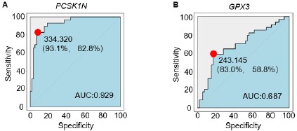
In the discussion, I think it would be valuable to summarise existing clinical/molecular predictors in PPGL and, acknowledging that their performance may be limited, compare them to the potential of these novel classifiers.
Thank you for your valuable suggestion. We have added a concise overview of established clinical and molecular predictors in PPGL and compared them with the potential of our transcriptional classifiers. The new paragraph (Discussion, lines 315–338) now reads:
“Compared to existing clinical and molecular predictors, risk assessment in PPGL has long relied on the following indicators: clinicopathological features (e.g., tumor size, non-adrenal origin, specific secretory phenotype, Ki-67 index), histopathological scoring systems (such as PASS/GAPP), and certain genetic alterations (including high-risk markers like SDHB inactivation mutations, as well as susceptibility gene mutations in ATRX, TERT promoter, MAML3, VHL, NF1, among others). Although these metrics are highly actionable in clinical practice, they exhibit several limitations: first, current molecular markers only cover a subset of patients, and technical constraints hinder the detection of many potentially significant variants (e.g., non-coding mutations), thereby compromising the comprehensiveness of prognostic evaluation; second, histopathological scoring is susceptible to interobserver variability; furthermore, the lack of standardized detection and evaluation protocols across institutions limits the comparability and generalizability of results. Our transcriptomic classification system—comprising C1 (pseudohypoxic/angiogenic signature), C2 (kinase-signaling signature), and C3 (SDHx-related signature)—provides a complementary approach to PPGL risk assessment. These subtypes reflect distinct biological backgrounds tied to specific genetic alterations and can be approximated by measuring the expression of individual genes (e.g., ANGPT2, PCSK1N, or GPX3). This study demonstrates that the classifier offers three major advantages: first, it accurately distinguishes subtypes with coherent biological features; second, it retains significant predictive value even after adjusting for clinical covariates; third, it can be implemented using readily available assays such as immunohistochemistry. These findings suggest that integrating transcriptomic subtyping with conventional clinical markers may offer a more comprehensive and generalizable risk stratification framework. However, this strategy would require validation through multi-center prospective studies and standardization of detection protocols.”
A little more explanation of the principles behind WGCNA would be useful in the methods.
We are grateful for your comments. We have expanded the Methods to briefly explain the principles of WGCNA (lines 426-454). In short, WGCNA constructs a weighted coexpression network from normalized gene expression, identifies modules of tightly co-expressed genes, summarizes each module by its eigengene (the first principal component), and then correlates module eigengenes with phenotypes (e.g., transcriptional subtypes) to highlight biologically meaningful gene sets and candidate hub genes. We now specify our preprocessing, choice of softthresholding power to approximate scale-free topology, module detection/merging criteria, and the statistics used for module–trait association and downstream gene-set scoring.
On line 234, I think the figure should be 5C?
We greatly appreciate your comments and Correct to Figure 5C.
when colonial explorers in Al-rica, Asia, and the Americas described species they encountered, the diversityof those species astonished and overwhelmed. When Linnaeus began his ca-reer, “natural history was a mess, and people needed guidelines,”
a
Dans le roman d’Asimov, les Solariens ont développé une véritable phobie des rapports directs, des rencontres en chair et en os.
L’auteur utilise la science-fiction pour illustrer la dérive possible : à force de virtualité, le contact réel devient menaçant.
Il n’empêche que cette crise sanitaire et les mesures imposées auront sans aucun doute contribué à en accélérer le processus.
La pandémie a fonctionné comme un accélérateur massif de l’hyperconnexion, rendant la virtualisation incontournable.
Bien sûr, nous n’avons pas attendu la pandémie de COVID-19 pour amorcer une transition vers un monde où le numérique s’impose de plus en plus, où les relations se virtualisent annihilant les distances géographiques, multipliant les possibilités de contacts immédiats tout en favorisant au quotidien l’évitement de contacts interpersonnels directs.
Janssen souligne que l’hyper-connexion n’est pas née avec le Covid : la pandémie n’a fait que révéler et amplifier une tendance déjà en cours.
Author response:
The following is the authors’ response to the original reviews
Reviewer #1 (Public review):
Weakness:
I wonder how task difficulty and linguistic labels interact with the current findings. Based on the behavioral data, shapes with more geometric regularities are easier to detect when surrounded by other shapes. Do shape labels that are readily available (e.g., "square") help in making accurate and speedy decisions? Can the sensitivity to geometric regularity in intraparietal and inferior temporal regions be attributed to differences in task difficulty? Similarly, are the MEG oddball detection effects that are modulated by geometric regularity also affected by task difficulty?
We see two aspects to the reviewer’s remarks.
(1) Names for shapes.
On the one hand, is the question of the impact of whether certain shapes have names and others do not in our task. The work presented here is not designed to specifically test the effect of formal western education; however, in previous work (Sablé-Meyer et al., 2021), we noted that the geometric regularity effect remains present even for shapes that do not have specific names, and even in participants who do not have names for them. Thus, we replicated our main effects with both preschoolers and adults that did not attend formal western education and found that our geometric feature model remained predictive of their behavior; we refer the reader to this previous paper for an extensive discussion of the possible role of linguistic labels, and the impact of the statistics of the environment on task performance.
What is more, in our behavior experiments we can discard data from any shape that is has a name in English and run our model comparison again. Doing so diminished the effect size of the geometric feature model, but it remained predictive of human behavior: indeed, if we removed all shapes but kite, rightKite, rustedHinge, hinge and random (i.e., more than half of our data, and shapes for which we came up with names but there are no established names), we nevertheless find that both models significantly correlate with human behavior—see plot in Author response image 1, equivalent of our Fig. 1E with the remaining shapes.
Author response image 1.
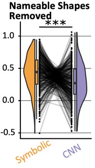
An identical analysis on the MEG leads to two noisy but significant clusters (CNN: 64.0ms to 172.0ms; then 192.0ms to 296.0ms; both p<.001: Geometric Features: 312.0ms to 364.0ms with p=.008). We have improved our manuscript thanks to the reviewer’s observation by adding a figure with the new behavior analysis to the supplementary figures and in the result section of the behavior task. We now refer to these analysis where appropriate:
(intro) “The effect appeared as a human universal, present in preschoolers, first-graders, and adults without access to formal western math education (the Himba from Namibia), and thus seemingly independent of education and of the existence of linguistic labels for regular shapes.”
(behavior results) “Finally, to separate the effect of name availability and geometric features on behavior, we replicated our analysis after removing the square, rectangle, trapezoids, rhombus and parallelogram from our data (Fig. S5D). This left us with five shapes, and an RDM with 10 entries, When regressing it in a GLM with our two models, we find that both models are still significant predictors (p<.001). The effect size of the geometric feature model is greatly reduced, yet remained significantly higher than that of the neural network model (p<.001).”
(meg results) “This analysis yielded similar clusters when performed on a subset of shapes that do not have an obvious name in English, as was the case for the behavior analysis (CNN Encoding: 64.0ms to 172.0ms; then 192.0ms to 296.0ms; both p<.001: Geometric Features: 312.0ms to 364.0ms with p=.008).”
(discussion, end of behavior section) “Previously, we only found such a significant mixture of predictors in uneducated humans (whether French preschoolers or adults from the Himba community, mitigating the possible impact of explicit western education, linguistic labels, and statistics of the environment on geometric shape representation) (Sablé-Meyer et al., 2021).”
Perhaps the referee’s point can also be reversed: we provide a normative theory of geometric shape complexity which has the potential to explain why certain shapes have names: instead of seeing shape names as the cause of their simpler mental representation, we suggest that the converse could occur, i.e. the simpler shapes are the ones that are given names.
(2) Task difficulty
On the other hand is the question of whether our effect is driven by task difficulty. First, we would like to point out that this point could apply to the fMRI task, which asks for an explicit detection of deviants, but does not apply to the MEG experiment. In MEG, participants passively looked at sequences of shapes which, for a given block, comprising many instances of a fixed standard shape and rare deviants–even if they notice deviants, they have no task related to them. Yet two independent findings validated the geometric features model: there was a large effect of geometric regularity on the MEG response to deviants, and the MEG dissimilarity matrix between standard shapes correlated with a model based on geometric features, better than with a model based on CNNs. While the response to rare deviants might perhaps be attributed to “difficulty” (assuming that, in spite of the absence of an explicit task, participants try to spot the deviants and find this self-imposed task more difficult in runs with less regular shapes), it seems very hard to explain the representational similarity analysis (RSA) findings based on difficulty. Indeed, what motivated us to use RSA analysis in both fMRI and MEG was to stop relying on the response to deviants, and use solely the data from standard or “reference” shapes, and model their neural response with theory-derived regressors.
We have updated the manuscript in several places to make our view on these points clearer:
(experiment 4) “This design allowed us to study the neural mechanisms of the geometric regularity effect without confounding effects of task, task difficulty, or eye movements.”
(figure 4, legend) “(A) Task structure: participants passively watch a constant stream of geometric shapes, one per second (presentation time 800ms). The stimuli are presented in blocks of 30 identical shapes up to scaling and rotation, with 4 occasional deviant shape. Participants do not have a task to perform beside fixating.”
Reviewer #2 (Public review):
Weakness:
Given that the primary take away from this study is that geometric shape information is found in the dorsal stream, rather than the ventral stream there is very little there is very little discussion of prior work in this area (for reviews, see Freud et al., 2016; Orban, 2011; Xu, 2018). Indeed, there is extensive evidence of shape processing in the dorsal pathway in human adults (Freud, Culham, et al., 2017; Konen & Kastner, 2008; Romei et al., 2011), children (Freud et al., 2019), patients (Freud, Ganel, et al., 2017), and monkeys (Janssen et al., 2008; Sereno & Maunsell, 1998; Van Dromme et al., 2016), as well as the similarity between models and dorsal shape representations (Ayzenberg & Behrmann, 2022; Han & Sereno, 2022).
We thank the reviewer for this opportunity to clarify our writing. We want to use this opportunity to highlight that our primary finding is not about whether the shapes of objects or animals (in general) are processed in the ventral versus or the dorsal pathway, but rather about the much more restricted domain of geometric shapes such as squares and triangles. We propose that simple geometric shapes afford additional levels of mental representation that rely on their geometric features – on top of the typical visual processing. To the best of our knowledge, this point has not been made in the above papers.
Still, we agree that it is useful to better link our proposal to previous ones. We have updated the discussion section titled “Two Visual Pathways” to include more specific references to the literature that have reported visual object representations in the dorsal pathway. Following another reviewer’s observation, we have also updated our analysis to better demonstrate the overlap in activation evoked by math and by geometry in the IPS, as well as include a novel comparison with independently published results.
Overall, to address this point, we (i) show the overlap between our “geometry” contrast (shape > word+tools+houses) and our “math” contrast (number > words); (ii) we display these ROIs side by side with ROIs found in previous work (Amalric and Dehaene, 2016), and (iii) in each math-related ROIs reported in that article, we test our “geometry” (shape > word+tools+houses) contrast and find almost all of them to be significant in both population; see Fig. S5.
Finally, within the ROIs identified with our geometry localizer, we also performed similarity analyses: for each region we extracted the betas of every voxel for every visual category, and estimated the distance (cross-validated mahalanobis) between different visual categories. In both ventral ROIs, in both populations, numbers were closer to shapes than to the other visual categories including text and Chinese characters (all p<.001). In adults, this result also holds for the right ITG (p=.021) and the left IPS (p=.014) but not the right IPS (p=.17). In children, this result did not hold in the areas.
Naturally, overlap in brain activation does not suffice to conclude that the same computational processes are involved. We have added an explicit caveat about this point. Indeed, throughout the article, we have been careful to frame our results in a way that is appropriate given our evidence, e.g. saying “Those areas are similar to those active during number perception, arithmetic, geometric sequences, and the processing of high-level math concepts” and “The IPS areas activated by geometric shapes overlap with those active during the comprehension of elementary as well as advanced mathematical concepts”. We have rephrased the possibly ambiguous “geometric shapes activated math- and number-related areas, particular the right aIPS.” into “geometric shapes activated areas independently found to be activated by math- and number-related tasks, in particular the right aIPS”.
Reviewer #3 (Public review):
Weakness:
Perhaps the manuscript could emphasize that the areas recruited by geometric figures but not objects are spatial, with reduced processing in visual areas. It also seems important to say that the images of real objects are interpreted as representations of 3D objects, as they activate the same visual areas as real objects. By contrast, the images of geometric forms are not interpreted as representations of real objects but rather perhaps as 2D abstractions.
This is an interesting possibility. Geometric shapes are likely to draw attention to spatial dimensions (e.g. length) and to do so in a 2D spatial frame of reference rather than the 3D representations evoked by most other objects or images. However, this possibility would require further work to be thoroughly evaluated, for instance by comparing usual 3D objects with rare instances of 2D ones (e.g. a sheet of paper, a sticker etc). In the absence of such a test, we refrained from further speculation on this point.
The authors use the term "symbolic." That use of that term could usefully be expanded here.
The reviewer is right in pointing out that “symbolic” should have been more clearly defined. We now added in the introduction:
(introduction) “[…] we sometimes refer to this model as “symbolic” because it relies on discrete, exact, rule-based features rather than continuous representations (Sablé-Meyer et al., 2022). In this representational format, geometric shapes are postulated to be represented by symbolic expressions in a “language-of-thought”, e.g. “a square is a four-sided figure with four equal sides and four right angles” or equivalently by a computer-like program from drawing them in a Logo-like language (Sablé-Meyer et al., 2022).”
Here, however, the present experiments do not directly probe this format of a representation. We have therefore simplified our wording and removed many of our use of the word “symbolic” in favor of the more specific “geometric features”.
Pigeons have remarkable visual systems. According to my fallible memory, Herrnstein investigated visual categories in pigeons. They can recognize individual people from fragments of photos, among other feats. I believe pigeons failed at geometric figures and also at cartoon drawings of things they could recognize in photos. This suggests they did not interpret line drawings of objects as representations of objects.
The comparison of geometric abilities across species is an interesting line of research. In the discussion, we briefly mention several lines of research that indicate that non-human primates do not perceive geometric shapes in the same way as we do – but for space reasons, we are reluctant to expand this section to a broader review of other more distant species. The referee is right that there is evidence of pigeons being able to perceive an invariant abstract 3D geometric shape in spite of much variation in viewpoint (Peissig et al., 2019) – but there does not seem to be evidence that they attend to geometric regularities specifically (e.g. squares versus non-squares). Also, the referee’s point bears on the somewhat different issue of whether humans and other animals may recognize the object depicted by a symbolic drawing (e.g. a sketch of a tree). Again, humans seem to be vastly superior in this domain, and research on this topic is currently ongoing in the lab. However, the point that we are making in the present work is specifically about the neural correlates of the representation of simple geometric shapes which by design were not intended to be interpretable as representations of objects.
Categories are established in part by contrast categories; are quadrilaterals, triangles, and circles different categories?
We are not sure how to interpret the referee’s question, since it bears on the definition of “category” (Spontaneous? After training? With what criterion?). While we are not aware of data that can unambiguously answer the reviewer’s question, categorical perception in geometric shapes can be inferred from early work investigating pop-out effects in visual search, e.g. (Treisman and Gormican, 1988): curvature appears to generate strong pop-out effects, and therefore we would expect e.g. circles to indeed be a different category than, say, triangles. Similarly, right angles, as well as parallel lines, have been found to be perceived categorically (Dillon et al., 2019).
This suggests that indeed squares would be perceived as categorically different from triangles and circles. On the other hand, in our own previous work (Sablé-Meyer et al., 2021) we have found that the deviants that we generated from our quadrilaterals did not pop out from displays of reference quadrilaterals. Pop-out is probably not the proper criterion for defining what a “category” is, but this is the extent to which we can provide an answer to the reviewer’s question.
It would be instructive to investigate stimuli that are on a continuum from representational to geometric, e.g., table tops or cartons under various projections, or balls or buildings that are rectangular or triangular. Building parts, inside and out. like corners. Objects differ from geometric forms in many ways: 3D rather than 2D, more complicated shapes, and internal texture. The geometric figures used are flat, 2-D, but much geometry is 3-D (e. g. cubes) with similar abstract features.
We agree that there is a whole line of potential research here. We decided to start by focusing on the simplest set of geometric shapes that would give us enough variation in geometric regularity while being easy to match on other visual features. We agree with the reviewer that our results should hold both for more complex 2-D shapes, but also for 3-D shapes. Indeed, generative theories of shapes in higher dimensions following similar principles as ours have been devised (I. Biederman, 1987; Leyton, 2003). We now mention this in the discussion:
“Finally, this research should ultimately be extended to the representation of 3-dimensional geometric shapes, for which similar symbolic generative models have indeed been proposed (Irving Biederman, 1987; Leyton, 2003).”
The feature space of geometry is more than parallelism and symmetry; angles are important, for example. Listing and testing features would be fascinating. Similarly, looking at younger or preferably non-Western children, as Western children are exposed to shapes in play at early ages.
We agree with the reviewer on all point. While we do not list and test the different properties separately in this work, we would like to highlight that angles are part of our geometric feature model, which includes features of “right-angle” and “equal-angles” as suggested by the reviewer.
We also agree about the importance of testing populations with limited exposure to formal training with geometric shapes. This was in fact a core aspect of a previous article of ours which tests both preschoolers, and adults with no access to formal western education – though no non-Western children (Sablé-Meyer et al., 2021). It remains a challenge to perform brain-imaging studies in non-Western populations (although see Dehaene et al., 2010; Pegado et al., 2014).
What in human experience but not the experience of close primates would drive the abstraction of these geometric properties? It's easy to make a case for elaborate brain processes for recognizing and distinguishing things in the world, shared by many species, but the case for brain areas sensitive to processing geometric figures is harder. The fact that these areas are active in blind mathematicians and that they are parietal areas suggests that what is important is spatial far more than visual. Could these geometric figures and their abstract properties be connected in some way to behavior, perhaps with fabrication and construction as well as use? Or with other interactions with complex objects and environments where symmetry and parallelism (and angles and curvature--and weight and size) would be important? Manual dexterity and fabrication also distinguish humans from great apes (quantitatively, not qualitatively), and action drives both visual and spatial representations of objects and spaces in the brain. I certainly wouldn't expect the authors to add research to this already packed paper, but raising some of the conceptual issues would contribute to the significance of the paper.
We refrained from speculating about this point in the previous version of the article, but share some of the reviewers’ intuitions about the underlying drive for geometric abstraction. As described in (Dehaene, 2026; Sablé-Meyer et al., 2022), our hypothesis, which isn’t tested in the present article, is that the emergence of a pervasive ability to represent aspects of the world as compact expressions in a mental “language-of-thought” is what underlies many domains of specific human competence, including some listed by the reviewer (tool construction, scene understanding) and our domain of study here, geometric shapes.
Recommendations for the Authors:
Reviewer #1 (Recommendations for the authors):
Overall, I enjoyed reading this paper. It is clearly written and nicely showcases the amount of work that has gone into conducting all these experiments and analyzing the data in sophisticated ways. I also thought the figures were great, and I liked the level of organization in the GitHub repository and am looking forward to seeing the shared data on OpenNeuro. I have some specific questions I hope the authors can address.
(1) Behavior
- Looking at Figure 1, it seemed like most shapes are clustering together, whereas square, rectangle, and maybe rhombus and parallelogram are slightly more unique. I was wondering whether the authors could comment on the potential influence of linguistic labels. Is it possible that it is easier to discard the intruder when the shapes are readily nameable versus not?
This is an interesting observation, but the existence of names for shapes does not suffice to explain all of our findings ; see our reply to the public comment.
(2) fMRI
- As mentioned in the public review, I was surprised that the authors went with an intruder task because I would imagine that performance depends on the specific combination of geometric shapes used within a trial. I assume it is much harder to find, for example, a "Right Hinge" embedded within "Hinge" stimuli than a "Right Hinge" amongst "Squares". In addition, the rotation and scaling of each individual item should affect regular shapes less than irregular shapes, creating visual dissimilarities that would presumably make the task harder. Can the authors comment on how we can be sure that the differences we pick up in the parietal areas are not related to task difficulty but are truly related to geometric shape regularities?
Again, please see our public review response for a larger discussion of the impact of task difficulty. There are two aspects to answering this question.
First, the task is not as the reviewer describes: the intruder task is to find a deviant shape within several slightly rotated and scaled versions of the regular shape it came from. During brain imaging, we did not ask participants to find an exemplar of one of our reference shape amidst copies of another, but rather a deviant version of one shape against copies of its reference version. We only used this intruder task with all pairs of shapes to generate the behavioral RSA matrix.
Second, we agree that some of the fMRI effect may stem from task difficulty, and this motivated our use of RSA analysis in fMRI, and a passive MEG task. RSA results cannot be explained by task difficulty.
Overall, we have tried to make the limitations of the fMRI design, and the motivation for turning to passive presentation in MEG, clearer by stating the issues more clearly when we introduce experiment 4:
“The temporal resolution of fMRI does not allow to track the dynamic of mental representations over time. Furthermore, the previous fMRI experiment suffered from several limitations. First, we studied six quadrilaterals only, compared to 11 in our previous behavioral work. Second, we used an explicit intruder detection, which implies that the geometric regularity effect was correlated with task difficulty, and we cannot exclude that this factor alone explains some of the activations in figure 3C (although it is much less clear how task difficulty alone would explain the RSA results in figure 3D). Third, the long display duration, which was necessary for good task performance especially in children, afforded the possibility of eye movements, which were not monitored inside the 3T scanner and again could have affected the activations in figure 3C.”
- How far in the periphery were the stimuli presented? Was eye-tracking data collected for the intruder task? Similar to the point above, I would imagine that a harder trial would result in more eye movements to find the intruder, which could drive some of the differences observed here.
A 1-degree bar was added to Figure 3A, which faithfully illustrates how the stimuli were presented in fMRI. Eye-tracking data was not collected during fMRI. Although the participants were explicitly instructed to fixate at the center of the screen and avoid eye movements, we fully agree with the referee that we cannot exclude that eye movements were present, perhaps more so for more difficult displays, and would therefore have contributed to the observed fMRI activations in experiment 3 (figure 3C). We now mention this limitation explicity at the end of experiment 3. However, crucially, this potential problem cannot apply to the MEG data. During the MEG task, the stimuli were presented one by one at the center of screen, without any explicit task, thus avoiding issues of eye movements. We therefore consider the MEG geometrical regularity effect, which comes at a relatively early latency (starting at ~160 ms) and even in a passive task, to provide the strongest evidence of geometric coding, unaffected by potential eye movement artefacts.
- I was wondering whether the authors would consider showing some un-thresholded maps just to see how widespread the activation of the geometric shapes is across all of the cortex.
We share the uncorrected threshold maps in Fig. S3. for both adults and children in the category localizer, copied here as well. For the geometry task, most of the clusters identified are fairly big and survive cluster-corrected permutations; the uncorrected statistical maps look almost fully identical to the one presented in Fig. 3 (p<.001 map).
- I'm missing some discussion on the role of early visual areas that goes beyond the RSA-CNN comparison. I would imagine that early visual areas are not only engaged due to top-down feedback (line 258) but may actually also encode some of the geometric features, such as parallel lines and symmetry. Is it feasible to look at early visual areas and examine what the similarity structure between different shapes looks like?
If early visual areas encoded the geometric features that we propose, then even early sensor-level RSA matrices should show a strong impact of geometric features similarity, which is not what we find (figure 4D). We do, however, appreciate the referee’s request to examine more closely how this similarity structure looks like. We now provide a movie showing the significant correlation between neural activity and our two models (uncorrected participants); indeed, while the early occipital activity (around 110ms) is dominated by a significant correlation with the CNN model, there are also scattered significant sources associated to the symbolic model around these timepoints already.
To test this further, we used beamformers to reconstruct the source-localized activity in calcarine cortex and performed an RSA analysis across that ROI. We find that indeed the CNN model is strongly significant at t=110ms (t=3.43, df=18, p=.003) while the geometric feature model is not (t=1.04, df=18, p=.31), and the CNN is significantly above the geometric feature model (t=4.25, df=18, p<.001). However, this result is not very stable across time, and there are significant temporal clusters around these timepoints associated to each model, with no significant cluster associated to a CNN > geometric (CNN: significant cluster from 88ms to 140ms, p<.001 in permutation based with 10000 permutations; geometric features has a significant cluster from 80ms to 104ms, p=.0475; no significant cluster on the difference between the two).
(3) MEG
- Similar to the fMRI set, I am a little worried that task difficulty has an effect on the decoding results, as the oddball should pop out more in more geometric shapes, making it easier to detect and easier to decode. Can the authors comment on whether it would matter for the conclusions whether they are decoding varying task difficulty or differences in geometric regularity, or whether they think this can be considered similarly?
See above for an extensive discussion of the task difficulty effect. We point out that there is no task in the MEG data collection part. We have clarified the task design by updating our Fig. 4. Additionally, the fact that oddballs are more perceived more or less easily as a function of their geometric regularity is, in part, exactly the point that we are making – but, in MEG, even in the absence of a task of looking for them.
- The authors discuss that the inflated baseline/onset decoding/regression estimates may occur because the shapes are being repeated within a mini-block, which I think is unlikely given the long ISIs and the fact that the geometric features model is not >0 at onset. I think their second possible explanation, that this may have to do with smoothing, is very possible. In the text, it said that for the non-smoothed result, the CNN encoding correlates with the data from 60ms, which makes a lot more sense. I would like to encourage the authors to provide readers with the unsmoothed beta values instead of the 100-ms smoothed version in the main plot to preserve the reason they chose to use MEG - for high temporal resolution!
We fully agree with the reviewer and have accordingly updated the figures to show the unsmoothed data (see below). Indeed, there is now no significant CNN effect before ~60 ms (up to the accuracy of identifying onsets with our method).
- In Figure 4C, I think it would be useful to either provide error bars or show variability across participants by plotting each participant's beta values. I think it would also be nice to plot the dissimilarity matrices based on the MEG data at select timepoints, just to see what the similarity structure is like.
Following the reviewer’s recommendation, we plot the timeseries with SEM as shaded area, and thicker lines for statistically significant clusters, and we provide the unsmoothed version in figure Fig. 4. As for the dissimilarity matrices at select timepoints, this has now been added to figure Fig. 4.
- To evaluate the source model reconstruction, I think the reader would need a little more detail on how it was done in the main text. How were the lead fields calculated? Which data was used to estimate the sources? How are the models correlated with the source data?
We have imported some of the details in the main text as follows (as well as expanding the methods section a little):
“To understand which brain areas generated these distinct patterns of activations, and probe whether they fit with our previous fMRI results, we performed a source reconstruction of our data. We projected the sensor activity onto each participant's cortical surfaces estimated from T1-images. The projection was performed using eLORETA and emptyroom recordings acquired on the same day to estimate noise covariance, with the default parameters of mne-bids-pipeline. Sources were spaced using a recursively subdivided octahedron (oct5). Group statistics were performed after alignement to fsaverage. We then replicated the RSA analysis […]”
- In addition to fitting the CNN, which is used here to model differences in early visual cortex, have the authors considered looking at their fMRI results and localizing early visual regions, extracting a similarity matrix, and correlating that with the MEG and/or comparing it with the CNN model?
We had ultimately decided against comparing the empirical similarity matrices from the MEG and fMRI experiments, first because the stimuli and tasks are different, and second because this would not be directly relevant to our goal, which is to evaluate whether a geometric-feature model accounts for the data. Thus, we systematically model empirical similarity matrices from fMRI and from MEG with our two models derived from different theories of shape perception in order to test predictions about their spatial and temporal dynamic. As for comparing the similarity matrix from early visual regions in fMRI with that predicted by the CNN model, this is effectively visible from our Fig. 3D where we perform searchlight RSA analysis and modeling with both the CNN and the geometric feature model; bilaterally, we find a correlation with the CNN model, although it sometimes overlap with predictions from the geometric feature model as well. We now include a section explaining this reasoning in appendix:
“Representational similarity analysis also offers a way to directly compared similarity matrices measured in MEG and fMRI, thus allowing for fusion of those two modalities and tentatively assigning a “time stamp” to distinct MRI clusters. However, we did not attempt such an analysis here for several reasons. First, distinct tasks and block structures were used in MEG and fMRI. Second, a smaller list of shapes was used in fMRI, as imposed by the slower modality of acquisition. Third, our study was designed as an attempt to sort out between two models of geometric shape recognition. We therefore focused all analyses on this goal, which could not have been achieved by direct MEG-fMRI fusion, but required correlation with independently obtained model predictions.”
Minor comments
- It's a little unclear from the abstract that there is children's data for fMRI only.
We have reworded the abstract to make this unambiguous
- Figures 4a & b are missing y-labels.
We can see how our labels could be confused with (sub-)plot titles and have moved them to make the interpretation clearer.
- MEG: are the stimuli always shown in the same orientation and size?
They are not, each shape has a random orientation and scaling. On top of a task example at the top of Fig. 4, we have now included a clearer mention of this in the main text when we introduce the task:
“shapes were presented serially, one at a time, with small random changes in rotation and scaling parameters, in miniblocks with a fixed quadrilateral shape and with rare intruders with the bottom right corner shifted by a fixed amount (Sablé-Meyer et al., 2021)”
- To me, the discussion section felt a little lengthy, and I wonder whether it would benefit from being a little more streamlined, focused, and targeted. I found that the structure was a little difficult to follow as it went from describing the result by modality (behavior, fMRI, MEG) back to discussing mostly aspects of the fMRI findings.
We have tried to re-organize and streamline the discussion following these comments.
Then, later on, I found that especially the section on "neurophysiological implementation of geometry" went beyond the focus of the data presented in the paper and was comparatively long and speculative.
We have reexamined the discussion, but the citation of papers emphasizing a representation of non-accidental geometric properties in non-human animals was requested by other commentators on our article; and indeed, we think that they are relevant in the context of our prior suggestion that the composition of geometric features might be a uniquely human feature – these papers suggest that individual features may not, and that it is therefore compositionality which might be special to the human brain. We have nevertheless shortened it.
Furthermore, we think that this section is important because symbolic models are often criticized for lack of a plausible neurophysiological implementation. It is therefore important to discuss whether and how the postulated symbolic geometric code could be realized in neural circuits. We have added this justification to the introduction of this section.
Reviewer #2 (Recommendations for the authors):
(1) If the authors want to specifically claim that their findings align with mathematical reasoning, they could at least show the overlap between the activation maps of the current study and those from prior work.
This was added to the fMRI results. See our answers to the public review.
(2) I wonder if the reason the authors only found aIPS in their first analysis (Figure 2) is because they are contrasting geometric shapes with figures that also have geometric properties. In other words, faces, objects, and houses also contain geometric shape information, and so the authors may have essentially contrasted out other areas that are sensitive to these features. One indication that this may be the case is that the geometric regularity effect and searchlight RSA (Figure 3) contains both anterior and posterior IPS regions (but crucially, little ventral activity). It might be interesting to discuss the implications of these differences.
Indeed, we cannot exclude that the few symmetries, perpendicularity and parallelism cues that can be presented in faces, objects or houses were processed as such, perhaps within the ventral pathway, and that these representations would have been subtracted out. We emphasize that our subtraction isolates the geometrical features that are present in simple regular geometric shapes, over and above those that might exist in other categories. We have added this point to the discussion:
“[… ] For instance, faces possess a plane of quasi-symmetry, and so do many other man-made tools and houses. Thus, our subtraction isolated the geometrical features that are present in simple regular geometric shapes (e.g. parallels, right angles, equality of length) over and above those that might already exist, in a less pure form, in other categories.”
(3) I had a few questions regarding the MEG results.
a. I didn't quite understand the task. What is a regular or oddball shape in this context? It's not clear what is being decoded. Perhaps a small example of the MEG task in Figure 4 would help?
We now include an additional sub-figure in Fig. 4 to explain the paradigm. In brief: there is no explicit task, participants are simply asked to fixate. The shapes come in miniblocks of 30 identical reference shapes (up to rotation and scaling), among which some occasional deviant shapes randomly appear (created by moving the corner of the reference shape by some amount).
b. In Figure 4A/B they describe the correlation with a 'symbolic model'. Is this the same as the geometric model in 4C?
It is. We have removed this ambiguity by calling it “geometric model” and setting its color to the one associated to this model thought the article.
c. The author's explanation for why geometric feature coding was slower than CNN encoding doesn't quite make sense to me. As an explanation, they suggest that previous studies computed "elementary features of location or motor affordance", whereas their study work examines "high-level mathematical information of an abstract nature." However, looking at the studies the authors cite in this section, it seems that these studies also examined the time course of shape processing in the dorsal pathway, not "elementary features of location or motor affordance." Second, it's not clear how the geometric feature model reflects high-level mathematical information (see point above about claiming this is related to math).
We thank the referee for pointing out this inappropriate phrase, which we removed. We rephrased the rest of the paragraph to clarify our hypothesis in the following way:
“However, in this work, we specifically probed the processing of geometric shapes that, if our hypothesis is correct, are represented as mental expressions that combine geometrical and arithmetic features of an abstract categorical nature, for instance representing “four equal sides” or “four right angles”. It seems logical that such expressions, combining number, angle and length information, take more time to be computed than the first wave of feedforward processing within the occipito-temporal visual pathway, and therefore only activate thereafter.”
One explanation may be that the authors' geometric shapes require finer-grained discrimination than the object categories used in prior studies. i.e., the odd-ball task may be more of a fine-grained visual discrimination task. Indeed, it may not be a surprise that one can decode the difference between, say, a hammer and a butterfly faster than two kinds of quadrilaterals.
We do not disagree with this intuition, although note that we do not have data on this point (we are reporting and modelling the MEG RSA matrix across geometric shapes only – in this part, no other shapes such as tools or faces are involved). Still, the difference between squares, rectangles, parallelograms and other geometric shapes in our stimuli is not so subtle. Furthermore, CNNs do make very fine grained distinctions, for instance between many different breeds of dogs in the IMAGENET corpus. Still, those sorts of distinctions capture the initial part of the MEG response, while the geometric model is needed only for the later part. Thus, we think that it is a genuine finding that geometric computations associated with the dorsal parietal pathway are slower than the image analysis performed by the ventral occipito-temporal pathway.
d. CNN encoding at time 0 is a little weird, but the author's explanation, that this is explained by the fact that temporal smoothed using a 100 ms window makes sense. However, smoothing by 100 ms is quite a lot, and it doesn't seem accurate to present continuous time course data when the decoding or RSA result at each time point reflects a 100 ms bin. It may be more accurate to simply show unsmoothed data. I'm less convinced by the explanation about shape prediction.
We agree. Following the reviewer’s advice, as well as the recommendation from reviewer 1, we now display unsmoothed plots, and the effects now exhibit a more reasonable timing (Figure 4D), with effects starting around ~60 ms for CNN encoding.
(4) I appreciate the author's use of multiple models and their explanation for why DINOv2 explains more variance than the geometric and CNN models (that it represents both types of features. A variance partitioning analysis may help strengthen this conclusion (Bonner & Epstein, 2018; Lescroart et al., 2015).
However, one difference between DINOv2 and the CNN used here is that it is trained on a dataset of 142 million images vs. the 1.5 million images used in ImageNet. Thus, DINOv2 is more likely to have been exposed to simple geometric shapes during training, whereas standard ImageNet trained models are not. Indeed, prior work has shown that lesioning line drawing-like images from such datasets drastically impairs the performance of large models (Mayilvahanan et al., 2024). Thus, it is unlikely that the use of a transformer architecture explains the performance of DINOv2. The authors could include an ImageNet-trained transformer (e.g., ViT) and a CNN trained on large datasets (e.g., ResNet trained on the Open Clip dataset) to test these possibilities. However, I think it's also sufficient to discuss visual experience as a possible explanation for the CNN and DINOv2 results. Indeed, young children are exposed to geometric shapes, whereas ImageNet-trained CNNs are not.
We agree with the reviewer’s observation. In fact, new and ongoing work from the lab is also exploring this; we have included in supplementary materials exactly what the reviewer is suggesting, namely the time course of the correlation with ViT and with ConvNeXT. In line with the reviewers’ prediction, these networks, trained on much larger dataset and with many more parameters, can also fit the human data as well as DINOv2. We ran additional analysis of the MEG data with ViT and ConvNeXT, which we now report in Fig. S6 as well as in an additional sentence in that section:
“[…] similar results were obtained by performing the same analysis, not only with another vision transformer network, ViT, but crucially using a much larger convolutional neural network, ConvNeXT, which comprises ~800M parameters and has been trained on 2B images, likely including many geometric shapes and human drawings. For the sake of completeness, RSA analysis in sensor space of the MEG data with these two models is provided in Fig. S6.”
We conclude that the size and nature of the training set could be as important as the architecture – but also note that humans do not rely on such a huge training set. We have updated the text, as well as Fig. S6, accordingly by updating the section now entitled “Vision Transformers and Larger Neural Networks”, and the discussion section on theoretical models.
(5) The authors may be interested in a recent paper from Arcaro and colleagues that showed that the parietal cortex is greatly expanded in humans (including infants) compared to non-human primates (Meyer et al., 2025), which may explain the stronger geometric reasoning abilities of humans.
A very interesting article indeed! We have updated our article to incorporate this reference in the discussion, in the section on visual pathways, as follows:
“Finally, recent work shows that within the visual cortex, the strongest relative difference in growth between human and non-human primates is localized in parietal areas (Meyer et al., 2025). If this expansion reflected the acquisition of new processing abilities in these regions, it might explain the observed differences in geometric abilities between human and non-human primates (Sablé-Meyer et al., 2021).”
Also, the authors may want to include this paper, which uses a similar oddity task and compelling shows that crows are sensitive to geometric regularity:
Schmidbauer, P., Hahn, M., & Nieder, A. (2025). Crows recognize geometric regularity. Science Advances, 11(15), eadt3718. https://doi.org/10.1126/sciadv.adt3718
We have ongoing discussions with the authors of this work and are have prepared a response to their findings (Sablé-Meyer and Dehaene, 2025)–ultimately, we think that this discussion, which we agree is important, does not have its place in the present article. They used a reduced version of our design, with amplified differences in the intruders. While they did not test the fit of their model with CNN or geometric feature models, we did and found that a simple CNN suffices to account for crow behavior. Thus, we disagree that their conclusions follow from their results and their conclusions. But the present article does not seem to be the right platform to engage in this discussion.
References
Ayzenberg, V., & Behrmann, M. (2022). The Dorsal Visual Pathway Represents Object-Centered Spatial Relations for Object Recognition. The Journal of Neuroscience, 42(23), 4693-4710. https://doi.org/10.1523/jneurosci.2257-21.2022
Bonner, M. F., & Epstein, R. A. (2018). Computational mechanisms underlying cortical responses to the affordance properties of visual scenes. PLoS Computational Biology, 14(4), e1006111. https://doi.org/10.1371/journal.pcbi.1006111
Bueti, D., & Walsh, V. (2009). The parietal cortex and the representation of time, space, number and other magnitudes. Philosophical Transactions of the Royal Society B: Biological Sciences, 364(1525), 1831-1840.
Dehaene, S., & Brannon, E. (2011). Space, time and number in the brain: Searching for the foundations of mathematical thought. Academic Press.
Freud, E., Culham, J. C., Plaut, D. C., & Bermann, M. (2017). The large-scale organization of shape processing in the ventral and dorsal pathways. eLife, 6, e27576.
Freud, E., Ganel, T., Shelef, I., Hammer, M. D., Avidan, G., & Behrmann, M. (2017). Three-dimensional representations of objects in dorsal cortex are dissociable from those in ventral cortex. Cerebral Cortex, 27(1), 422-434.
Freud, E., Plaut, D. C., & Behrmann, M. (2016). 'What 'is happening in the dorsal visual pathway. Trends in Cognitive Sciences, 20(10), 773-784.
Freud, E., Plaut, D. C., & Behrmann, M. (2019). Protracted developmental trajectory of shape processing along the two visual pathways. Journal of Cognitive Neuroscience, 31(10), 1589-1597.
Han, Z., & Sereno, A. (2022). Modeling the Ventral and Dorsal Cortical Visual Pathways Using Artificial Neural Networks. Neural Computation, 34(1), 138-171. https://doi.org/10.1162/neco_a_01456
Janssen, P., Srivastava, S., Ombelet, S., & Orban, G. A. (2008). Coding of shape and position in macaque lateral intraparietal area. Journal of Neuroscience, 28(26), 6679-6690.
Konen, C. S., & Kastner, S. (2008). Two hierarchically organized neural systems for object information in human visual cortex. Nature Neuroscience, 11(2), 224-231.
Lescroart, M. D., Stansbury, D. E., & Gallant, J. L. (2015). Fourier power, subjective distance, and object categories all provide plausible models of BOLD responses in scene-selective visual areas. Frontiers in Computational Neuroscience, 9(135), 1-20. https://doi.org/10.3389/fncom.2015.00135
Mayilvahanan, P., Zimmermann, R. S., Wiedemer, T., Rusak, E., Juhos, A., Bethge, M., & Brendel, W. (2024). In search of forgotten domain generalization. arXiv Preprint arXiv:2410.08258.
Meyer, E. E., Martynek, M., Kastner, S., Livingstone, M. S., & Arcaro, M. J. (2025). Expansion of a conserved architecture drives the evolution of the primate visual cortex. Proceedings of the National Academy of Sciences, 122(3), e2421585122. https://doi.org/10.1073/pnas.2421585122
Orban, G. A. (2011). The extraction of 3D shape in the visual system of human and nonhuman primates. Annual Review of Neuroscience, 34, 361-388.
Romei, V., Driver, J., Schyns, P. G., & Thut, G. (2011). Rhythmic TMS over Parietal Cortex Links Distinct Brain Frequencies to Global versus Local Visual Processing. Current Biology, 21(4), 334-337. https://doi.org/10.1016/j.cub.2011.01.035
Sereno, A. B., & Maunsell, J. H. R. (1998). Shape selectivity in primate lateral intraparietal cortex. Nature, 395(6701), 500-503. https://doi.org/10.1038/26752
Summerfield, C., Luyckx, F., & Sheahan, H. (2020). Structure learning and the posterior parietal cortex. Progress in Neurobiology, 184, 101717. https://doi.org/10.1016/j.pneurobio.2019.101717
Van Dromme, I. C., Premereur, E., Verhoef, B.-E., Vanduffel, W., & Janssen, P. (2016). Posterior Parietal Cortex Drives Inferotemporal Activations During Three-Dimensional Object Vision. PLoS Biology, 14(4), e1002445. https://doi.org/10.1371/journal.pbio.1002445
Xu, Y. (2018). A tale of two visual systems: Invariant and adaptive visual information representations in the primate brain. Annu. Rev. Vis. Sci, 4, 311-336.
Reviewer #3 (Recommendations for the authors):
Bring into the discussion some of the issues outlined above, especially a) the spatial rather than visual of the geometric figures and b) the non-representational aspects of geometric form aspects.
We thank the reviewer for their recommendations – see our response to the public review for more details.
Note: This response was posted by the corresponding author to Review Commons. The content has not been altered except for formatting.
Learn more at Review Commons
Reviewer #1
Evidence, reproducibility and clarity
This paper addresses a very interesting problem of non-centrosomal microtubule organization in developing Drosophila oocytes. Using genetics and imaging experiments, the authors reveal an interplay between the activity of kinesin-1, together with its essential cofactor Ensconsin, and microtubule organization at the cell cortex by the spectraplakin Shot, minus-end binding protein Patronin and Ninein, a protein implicated in microtubule minus end anchoring. The authors demonstrate that the loss of Ensconsin affects the cortical accumulation non-centrosomal microtubule organizing center (ncMTOC) proteins, microtubule length and vesicle motility in the oocyte, and show that this phenotype can be rescued by constitutively active kinesin-1 mutant, but not by Ensconsin mutants deficient in microtubule or kinesin binding. The functional connection between Ensconsin, kinesin-1 and ncMTOCs is further supported by a rescue experiment with Shot overexpression. Genetics and imaging experiments further implicate Ninein in the same pathway. These data are a clear strength of the paper; they represent a very interesting and useful addition to the field.
The weaknesses of the study are two-fold. First, the paper seems to lack a clear molecular model, uniting the observed phenomenology with the molecular functions of the studied proteins. Most importantly, it is not clear how kinesin-based plus-end directed transport contributes to cortical localization of ncMTOCs and regulation of microtubule length.
Second, not all conclusions and interpretations in the paper are supported by the presented data.
We thank the reviewer for recognizing the impact of this work. In response to the insightful suggestions, we performed extensive new experiments that establish a well-supported cellular and molecular model (Figure 7). The discussion has been restructured to directly link each conclusion to its corresponding experimental evidence, significantly strengthening the manuscript.
Below is a list of specific comments, outlining the concerns, in the order of appearance in the paper/figures.
Figure 1. The statement: "Ens loading on MTs in NCs and their subsequent transport by Dynein toward ring canals promotes the spatial enrichment of the Khc activator Ens in the oocyte" is not supported by data. The authors do not demonstrate that Ens is actually transported from the nurse cells to the oocyte while being attached to microtubules. They do show that the intensity of Ensconsin correlates with the intensity of microtubules, that the distribution of Ensconsin depends on its affinity to microtubules and that an Ensconsin pool locally photoactivated in a nurse cell can redistribute to the oocyte (and throughout the nurse cell) by what seems to be diffusion. The provided images suggest that Ensconsin passively diffuses into the oocyte and accumulates there because of higher microtubule density, which depends on dynein. To prove that Ensconsin is indeed transported by dynein in the microtubule-bound form, one would need to measure the residence time of Ensconsin on microtubules and demonstrate that it is longer than the time needed to transport microtubules by dynein into the oocyte; ideally, one would like to see movement of individual microtubules labelled with photoconverted Ensconsin from a nurse cell into the oocyte. Since microtubules are not enriched in the oocyte of the dynein mutant, analysis of Ensconsin intensity in this mutant is not informative and does not reveal the mechanism of Ensconsin accumulation.
As noted by Reviewer 3, the directional movement of microtubules traveling at ~140 nm/s from nurse cells toward the oocyte through Ring Canals was previously reported using a tagged Ens-MT binding domain reporter line by Lu et al. (2022). We have therefore added the citation of this crucial work in the novel version of the manuscript (lane 155-157) and removed the photo-conversion panel.
Critically, however, our study provides mechanistic insight that was missing from this earlier work: this mechanism is also crucial to enrich MAPs in the oocyte. The fact that Dynein mutants fail to enrich Ensconsin is a crucial piece of evidence: it supports a model of Ensconsin-loaded MT transport (Figure 1D-1F).
Figure 2. According to the abstract, this figure shows that Ensconsin is "maintained at the oocyte cortex by Ninein". However, the figure doesn't seem to prove it - it shows that oocyte enrichment of Ensonsin is partially dependent on Ninein, but this applies to the whole cell and not just to the cell cortex. Furthermore, it is not clear whether Ninein mutation affects microtubule density, which in turn would affect Ensconsin enrichment, and therefore, it is not clear whether the effect of Ninein loss on Ensconsin distribution is direct or indirect.
Ninein plays a critical role in Ensconsin enrichment and microtubule organization in the oocyte (new Figure 2, Figure 3, Figure S3). Quantification of total Tubulin signal shows no difference between control and Nin mutant oocytes (new Figure S3 panels A, B). We found decreased Ens enrichment in the oocyte, and Ens localization on MTs and to the cell cortex (Figure 2E, 2F, and Figure S3C and S3D).
Novel quantitative analyses of microtubule orientation at the anterior cortex, where MTs are normally preferentially oriented toward the posterior pole (Parton et al. 2011), demonstrate that Nin mutants exhibit randomized MT orientation compared to wild-type oocytes (new Figure 3C-3E).These findings establish that Ninein (although not essential) favors Ensconsin localization on MTs, Ens enrichment in the oocyte, ncMTOC cortical localization, and more robust MT orientation toward the posterior cortex. It also suggests that Ens levels in the oocyte acts as a rheostat to control Khc activation.
The observation that the aggregates formed by overexpressed Ninein accumulate other proteins, including Ensconsin, supports, though does not prove their interactions. Furthermore, there is absolutely no proof that Ninein aggregates are "ncMTOCs". Unless the authors demonstrate that these aggregates nucleate or anchor microtubules (for example, by detailed imaging of microtubules and EB1 comets), the text and labels in the figure would need to be altered.
We have modified the manuscript, we now refer to an accumulation of these components in large puncta, rather than aggregates, consistent with previous observations (Rosen et al., 2000). We acknowledge in the revised version that these puncta recruit Shot, Patronin and Ens without mentioning direct interaction (lane 218).
Importantly, we conducted a more detailed characterization of these Ninein/Shot/Patronin/Ens-containing puncta in a novel Figure S4. To rigorously assess their nucleation capacity, we analyzed Eb1-GFP-labeled MT comets, a robust readout of MT nucleation (Parton et al., 2011, Nashchekin et al., 2016). While few Eb1-positive comets occasionally emanate from these structures, confirming their identity as putative ncMTOCs, these puncta function as surprisingly weak nucleation centers (new Figure S4 E, Video S1) and, their presence does not alter overall MT architecture (new Figure S4 F). Moreover, these puncta disappear over time, are barely visible at stage 10B, they do not impair oocyte development or fertility (Figure S4 G and Table 1).
Minor comment: Note that a "ratio" (Figure 2C) is just a ratio, and should not be expressed in arbitrary units.
We have amended this point in all the figures.
Figure 3B: immunoprecipitation results cannot be interpreted because the immunoprecipitated proteins (GFP, Ens-GFP, Shot-YFP) are not shown. It is also not clear that this biochemical experiment is useful. If the authors would like to suggest that Ensconsin directly binds to Patronin, the interaction would need to be properly mapped at the protein domain level.
This is a good point: the GFP and Ens-GFP immunoprecipitated proteins are now much clearly identified on the blots and in the figure legend (new Figure 4G). Shot-YFP IP, was used as a positive control but is difficult to be detected by Western blot due to its large size (>106 Da) using conventional acrylamide gels (Nashchekin et al., 2016).
We now explicitly state that immunoprecipitations were performed at 4°C, where microtubules are fully depolymerized, thereby excluding undirect microtubule-mediated interactions. We agree with this reviewer: we cannot formally rule out interactions through bridging by other protein components. This is stated in the revised manuscript (lane 238-239).
One of the major phenotypes observed by the authors in Ens mutant is the loss of long microtubules. The authors make strong conclusions about the independence of this phenotype from the parameters of microtubule plus-end growth, but in fact, the quality of their data does not allow to make such a conclusion, because they only measured the number of EB1 comets and their growth rate but not the catastrophe, rescue or pausing frequency."Note that kinesin-1 has been implicated in promoting microtubule damage and rescue (doi: 10.1016/j.devcel.2021).In the absence of such measurements, one cannot conclude whether short microtubules arise through defects in the minus-end, plus-end or microtubule shaft regulation pathways.
We thank the reviewer for raising this important point. Our data demonstrate that microtubule (MT) nucleation and polymerization rates remain unaffected under Khc RNAi and ens mutant conditions, indicating that MT dynamics alterations must arise through alternative mechanisms.
As the reviewer suggested, recent studies on Kinesin activity and MT network regulation are indeed highly relevant. Two key studies from the Verhey and Aumeier laboratories examined Kinesin-1 gain-of-function conditions and revealed that constitutively active Kinesin-1 induces MT lattice damage (Budaitis et al., 2022). While damaged MTs can undergo self-repair, Aumeier and colleagues demonstrated that GTP-tubulin incorporation generates "rescue shafts" that promote MT rescue events (Andreu-Carbo et al., 2022). Extrapolating from these findings, loss of Kinesin-1 activity could plausibly reduce rescue shaft formation, thereby decreasing MT rescue frequency and stability. Although this hypothesis is challenging to test directly in our system, it provides a mechanistic framework for the observed reduction in MT number and stability.
Additionally, the reviewer highlighted the role of Khc in transporting the dynactin complex, an anti-catastrophe factor, to MT plus ends (Nieuwburg et al., 2017), which could further contribute to MT stabilization. This crucial reference is now incorporated into the revised Discussion.
Importantly, our work also demonstrates the contribution of Ens/Khc to ncMTOC targeting to the cell cortex. Our new quantitative analyses of MT organization (new Figure 5 B) reveal a defective anteroposterior orientation of cortical MTs in mutant conditions, pointing to a critical role for cortical ncMTOCs in organizing the MT network.
Taken together, we propose that the observed MT reduction and disorganization result from multiple interconnected mechanisms: (1) reduced rescue shaft formation affecting MT stability; (2) impaired transport of anti-catastrophe factors to MT plus ends; and (3) loss of cortical ncMTOCs, which are essential for minus-end MT stabilization and network organization. The Discussion has been revised to reflect this integrated model in a dedicated paragraph (“A possible regulation of MT dynamics in the oocyte at both plus end minus MT ends by Ens and Khc” lane 415-432).
It is important to note in that a spectraplakin, like Shot, can potentially affect different pathways, particularly when overexpressed.
We agree that Shot harbors multiple functional domains and acts as a key organizer of both actin and microtubule cytoskeletons. Overexpression of such a cytoskeletal cross-linker could indeed perturb both networks, making interpretation of Ens phenotype rescue challenging due to potential indirect effects.
To address this concern, we selected an appropriate Shot isoform for our rescue experiments that displayed similar localization to “endogenous” Shot-YFP (a genomic construct harboring shot regulatory sequences) and importantly that was not overexpressed.
Elevated expression of the Shot.L(A) isoform (see Western Blot Figure S8 A), considered as the wild-type form with two CH1 and CH2 actin-binding motifs (Lee and Kolodziej, 2002), showed abnormal localization such as strong binding to the microtubules in nurse cells and oocyte confirming the risk of gain-of-function artifacts and inappropriate conclusions (Figure S8 B, arrows).
By contrast, our rescue experiments using the Shot.L(C) isoform (that only harbors the CH2 motif) provide strong evidence against such artifacts for three reasons. First, Shot-L(C) is expressed at slightly lower levels than a Shot-YFP genomic construct (not overexpressed), and at much lower levels than Shot-L(A), despite using the same driver (Figure S8 A). Second, Shot-L(C) localization in the oocyte is similar to that of endogenous Shot-YFP, concentrating at the cell cortex (Figure S8 B, compare lower and top panels). Taken together, these controls rather suggest our rescue with the Shot-L(C) is specific.
Note that this Shot-L(C) isoform is sufficient to complement the absence of the shot gene in other cell contexts (Lee and Kolodziej, 2002).
Unjustified conclusions should be removed: the authors do not provide sufficient data to conclude that "ens and Khc oocytes MT organizational defects are caused by decreased ncMTOC cortical anchoring", because the actual cortical microtubule anchoring was not measured.
This is a valid point. We acknowledge that we did not directly measure microtubule anchoring in this study. In response, we have revised the discussion to more accurately reflect our observations. Throughout the manuscript, we now refer to "cortical microtubule organization" rather than "cortical microtubule anchoring," which better aligns with the data presented.
Minor comment: Microtubule growth velocity must be expressed in units of length per time, to enable evaluating the quality of the data, and not as a normalized value.
This is now amended in the revised version (modified Figure S7).
A significant part of the Discussion is dedicated to the potential role of Ensconsin in cortical microtubule anchoring and potential transport of ncMTOCs by kinesin. It is obviously fine that the authors discuss different theories, but it would be very helpful if the authors would first state what has been directly measured and established by their data, and what are the putative, currently speculative explanations of these data.
We have carefully considered the reviewer's constructive comments and are confident that this revised version fully addresses their concerns.
First, we have substantially strengthened the connection between the Results and Discussion sections, ensuring that our interpretations are more directly anchored in the experimental data. This restructuring significantly improves the overall clarity and logical flow of the manuscript.
Second, we have added a new comprehensive figure presenting a molecular-scale model of Kinesin-1 activation upon release of autoinhibition by Ensconsin (new Figure 7D). Critically, this figure also illustrates our proposed positive feedback loop mechanism: Khc-dependent cytoplasmic advection promotes cortical recruitment of additional ncMTOCs, which generates new cortical microtubules and further accelerates cytoplasmic transport (Figure 7 A-C). This self-amplifying cycle provides a mechanistic framework consistent with emerging evidence that cytoplasmic flows are essential for efficient intracellular transport in both insect and mammalian oocytes.
Minor comment: The writing and particularly the grammar need to be significantly improved throughout, which should be very easy with current language tools. Examples: "ncMTOCs recruitment" should be "ncMTOC recruitment"; "Vesicles speed" should be "Vesicle speed", "Nin oocytes harbored a WT growth,"- unclear what this means, etc. Many paragraphs are very long and difficult to read. Making shorter paragraphs would make the authors' line of thought more accessible to the reader.
We have amended and shortened the manuscript according to this reviewer feed-back. We have specifically built more focused paragraphs to facilitates the reading.
Significance
This paper represents significant advance in understanding non-centrosomal microtubule organization in general and in developing Drosophila oocytes in particular by connecting the microtubule minus-end regulation pathway to the Kinesin-1 and Ensconsin/MAP7-dependent transport. The genetics and imaging data are of good quality, are appropriately presented and quantified. These are clear strengths of the study which will make it interesting to researchers studying the cytoskeleton, microtubule-associated proteins and motors, and fly development.
The weaknesses of this study are due to the lack of clarity of the overall molecular model, which would limit the impact of the study on the field. Some interpretations are not sufficiently supported by data, but this can be solved by more precise and careful writing, without extensive additional experimentation.
We thank the reviewer for raising these important concerns regarding clarity and data interpretation. We have thoroughly revised the manuscript to address these issues on multiple fronts. First, we have substantially rewritten key sections to ensure that our conclusions are clearly articulated and directly supported by the data. Second, we have performed several new experiments that now allow us to propose a robust mechanistic model, presented in new figures. These additions significantly strengthen the manuscript and directly address the reviewer's concerns.
My expertise is cell biology and biochemistry of the microtubule cytoskeleton, including both microtubule-associated proteins and microtubule motors.
Reviewer #2
Evidence, reproducibility and clarity
In this manuscript, Berisha et al. investigate how microtubule (MT) organization is spatially regulated during Drosophila oogenesis. The authors identify a mechanism in which the Kinesin-1 activator Ensconsin/MAP7 is transported by dynein and anchored at the oocyte cortex via Ninein, enabling localized activation of Kinesin-1. Disruption of this pathway impairs ncMTOC recruitment and MT anchoring at the cortex. The authors combine genetic manipulation with high-resolution microscopy and use three key readouts to assess MT organization during mid-to-late oogenesis: cortical MT formation, localization of posterior determinants, and ooplasmic streaming. Notably, Kinesin-1, in concert with its activator Ens/MAP7, contributes to organizing the microtubule network it travels along. Overall, the study presents interesting findings, though we have several concerns we would like the authors to address. Ensconsin enrichment in the oocyte 1. Enrichment in the oocyte • Ensconsin is a MAP that binds MTs. Given that microtubule density in the oocyte significantly exceeds that in the nurse cells, its enrichment may passively reflect this difference. To assess whether the enrichment is specific, could the authors express a non-Drosophila MAP (e.g., mammalian MAP1B) to determine whether it also preferentially localizes to the oocyte?
To address this point, we performed a new series of experiments analyzing the enrichment of other Drosophila and non-Drosophila MAPs, including Jupiter-GFP, Eb1-GFP, and bovine Tau-GFP, all widely used markers of the microtubule cytoskeleton in flies (see new Figure S2). Our results reveal that Jupiter-GFP, Eb1-GFP, and bovine Tau-GFP all exhibit significantly weaker enrichment in the oocyte compared to Ens-GFP. Khc-GFP also shows lower enrichment. These findings indicate that MAP enrichment in the oocyte is MAP-dependent, rather than solely reflecting microtubule density or organization. Of note, we cannot exclude that microtubule post-translational modifications contribute to differential MAP binding between nurse cells and the oocyte, but this remains a question for future investigation.
The ability of ens-wt and ens-LowMT to induce tubulin polymerization according to the light scattering data (Fig. S1J) is minimal and does not reflect dramatic differences in localization. The authors should verify that, in all cases, the polymerization product in their in vitro assays is microtubules rather than other light-scattering aggregates. What is the control in these experiments? If it is just purified tubulin, it should not form polymers at physiological concentrations.
The critical concentration Cr for microtubule self-assembly in classical BRB80 buffer found by us and others is around 20 µM (see Fig. 2c in Weiss et al., 2010). Here, microtubules were assembled at 40 µM tubulin concentration, i.e., largely above the Cr. As stated in the materials and methods section, we systematically induced cooling at 4°C after assembly to assess the presence of aggregates, since those do not fall apart upon cooling. The decrease in optical density upon cooling is a direct control that the initial increase in DO is due to the formation of microtubules. Finally, aggregation and polymerization curves are widely different, the former displaying an exponential shape and the latter a sigmoid assembly phase (see Fig. 3A and 3B in Weiss et al., 2010).
Photoconversion caveatsMAPs are known to dynamically associate and dissociate from microtubules. Therefore, interpretation of the Ens photoconversion data should be made with caution. The expanding red signal from the nurse cells to the oocyte may reflect a any combination of dynein-mediated MT transport and passive diffusion of unbound Ensconsin. Notably, photoconversion of a soluble protein in the nurse cells would also result in a gradual increase in red signal in the oocyte, independent of active transport. We encourage the authors to more thoroughly discuss these caveats. It may also help to present the green and red channels side by side rather than as merged images, to allow readers to assess signal movement and spatial patterns better.
This is a valid point that mirrors the comment of Reviewers 1 and 3. The directional movement of microtubules traveling at ~140 nm/s from nurse cells toward the oocyte via the ring canals was previously reported by Lu et al. (2022) with excellent spatial resolution. Notably, this MT transport was measured using a fusion protein containing the Ens MT-binding domain. We now cite this relevant study in our revised manuscript and have removed this redundant panel in Figure 1.
Reduction of Shot at the anterior cortex• Shot is known to bind strongly to F-actin, and in the Drosophila ovary, its localization typically correlates more closely with F-actin structures than with microtubules, despite being an MT-actin crosslinker. Therefore, the observed reduction of cortical Shot in ens, nin mutants, and Khc-RNAi oocytes is unexpected. It would be important to determine whether cortical F-actin is also disrupted in these conditions, which should be straightforward to assess via phalloidin staining.
As requested by the reviewer, we performed actin staining experiments, which are now presented in a new Figure S5. These data demonstrate that the cortical actin network remains intact in all mutant backgrounds analyzed, ruling out any indirect effect of actin cytoskeleton disruption on the observed phenotypes.
MTs are barely visible in Fig. 3A, which is meant to demonstrate Ens-GFP colocalization with tubulin. Higher-quality images are needed.
The revised version now provides significantly improved images to show the different components examined. Our data show that Ens and Ninein localize at the cell cortex where they co-localize with Shot and Patronin (Figure 2 A-C). In addition, novel images show that Ens extends along microtubules (new Figure 4 A).
MT gradient in stage 9 oocytesIn ens-/-, nin-/-, and Khc-RNAi oocytes, is there any global defect in the stage 9 microtubule gradient? This information would help clarify the extent to which cortical localization defects reflect broader disruptions in microtubule polarity.
We now provide quantitative analysis of microtubule (MT) array organization in novel figures (Figure 3D and Figure 5B). Our data reveal that both Khc RNAi and ens mutant oocytes exhibit severe disruption of MT orientation toward the posterior (new Figure 5B). Importantly, this defect is significantly less pronounced in Nin-/- oocytes, which retain residual ncMTOCs at the cortex (new Figure 3D). This differential phenotype supports our model that cortical ncMTOCs are critical for maintaining proper MT orientation toward the posterior side of the oocyte.
Role of Ninein in cortical anchoringThe requirement for Ninein in cortical anchorage is the least convincing aspect of the manuscript and somewhat disrupts the narrative flow. First, it is unclear whether Ninein exhibits the same oocyte-enriched localization pattern as Ensconsin. Is Ninein detectable in nurse cells? Second, the Ninein antibody signal appears concentrated in a small area of the anterior-lateral oocyte cortex (Fig. 2A), yet Ninein loss leads to reduced Shot signal along a much larger portion of the anterior cortex (Fig. 2F)-a spatial mismatch that weakens the proposed functional relationship. Third, Ninein overexpression results in cortical aggregates that co-localize with Shot, Patronin, and Ensconsin. Are these aggregates functional ncMTOCs? Do microtubules emanate from these foci?
We now provide a more comprehensive analysis of Ninein localization. Similar to Ensconsin (Ens), endogenous Ninein is enriched in the oocyte during the early stages of oocyte development but is also detected in NCs (see modified Figure 2 A and Lasko et al., 2016). Improved imaging of Ninein further shows that the protein partially co-localizes with Ens, and ncMTOCs at the anterior cortex and with Ens-bound MTs (Figure 2B, 2C).
Importantly, loss of Ninein (Nin) only partially reduces the enrichment of Ens in the oocyte (Figure 2E). Both Ens and Kinesin heavy chain (Khc) remain partially functional and continue to target non-centrosomal microtubule-organizing centers (ncMTOCs) to the cortex (Figure 3A). In Nin-/- mutants, a subset of long cortical microtubules (MTs) is present, thereby generating cytoplasmic streaming, although less efficiently than under wild-type (WT) conditions (Figure 3F and 3G). As a non-essential gene, we envisage Ninein as a facilitator of MT organization during oocyte development.
Finally, our new analyses demonstrate that large puncta containing Ninein, Shot, Patronin, and despite their size, appear to be relatively weak nucleation centers (revised Figure S4 E and Video 1). In addition, their presence does not bias overall MT architecture (Figure S4 F) nor impair oocyte development and fertility (Figure S4 G and Table 1).
Inconsistency of Khc^MutEns rescueThe Khc^MutEns variant partially rescues cortical MT formation and restores a slow but measurable cytoplasmic flow yet it fails to rescue Staufen localization (Fig. 5). This raises questions about the consistency and completeness of the rescue. Could the authors clarify this discrepancy or propose a mechanistic rationale?
This is a good point. The cytoplasmic flows (the consequence of cargo transport by Khc on MTs) generated by a constitutively active KhcMutEns in an ens mutant condition, are less efficient than those driven by Khc activated by Ens in a control condition (Figure 6C). The rescued flow is probably not efficient enough to completely rescue the Staufen localization at stage 10.
Additionally, this KhcMutEns variant rescues the viability of embryos from Khc27 mutant germline clones oocytes but not from ens mutants (Table1). One hypothesis is that Ens harbors additional functions beyond Khc activation.
This incomplete rescue of Ens by an active Khc variant could also be the consequence of the “paradox of co-dependence”: Kinesin-1 also transport the antagonizing motor Dynein that promotes cargo transport in opposite directions (Hancock et al., 2016). The phenotype of a gain of function variant is therefore complex to interpret. Consistent with this, both KhcMutEns-GFP and KhcDhinge2 two active Khc only rescues partially centrosome transport in ens mutant Neural Stem Cells (Figure S10).
Minor points: 1. The pUbi-attB-Khc-GFP vector was used to generate the Khc^MutEns transgenic line, presumably under control of the ubiquitous ubi promoter. Could the authors specify which attP landing site was used? Additionally, are the transgenic flies viable and fertile, given that Kinesin-1 is hyperactive in this construct?
All transgenic constructs were integrated at defined genomic landing sites to ensure controlled expression levels. Specifically, both GFP-tagged KhcWT and KhcMutEns were inserted at the VK05 (attP9A) site using PhiC31-mediated integration. Full details of the landing sites are provided in the Materials and Methods section. Both transgenic flies are homozygous lethal and the transgenes are maintained over TM6B balancers.
On page 11 (Discussion, section titled "A dual Ensconsin oocyte enrichment mechanism achieves spatial relief of Khc inhibition"), the statement "many mutations in Kif5A are causal of human diseases" would benefit from a brief clarification. Since not all readers may be familiar with kinesin gene nomenclature, please indicate that KIF5A is one of the three human homologs of Kinesin heavy chain.
We clarified this point in the revised version (lane 465-466).
On page 16 (Materials and Methods, "Immunofluorescence in fly ovaries"), the sentence "Ovaries were mounted on a slide with ProlonGold medium with DAPI (Invitrogen)" should be corrected to "ProLong Gold."
This is corrected.
Significance
This study shows that enrichment of MAP7/ensconsin in the oocyte is the mechanism of kinesin-1 activation there and is important for cytoplasmic streaming and localization non-centrosomal microtubule-organizing centers to the oocyte cortex
We thank the reviewers for the accurate review of our manuscript and their positive feed-back.
Reviewer #3
Evidence, reproducibility and clarity
The manuscript of Berisha et al., investigates the role of Ensconsin (Ens), Kinesin-1 and Ninein in organisation of microtubules (MT) in Drosophila oocyte. At stage 9 oocytes Kinesin-1 transports oskar mRNA, a posterior determinant, along MT that are organised by ncMTOCs. At stage 10b, Kinesin-1 induces cytoplasmic advection to mix the contents of the oocyte. Ensconsin/Map7 is a MT associated protein (MAP) that uses its MT-binding domain (MBD) and kinesin binding domain (KBD) to recruit Kinesin-1 to the microtubules and to stimulate the motility of MT-bound Kinesin-1. Using various new Ens transgenes, the authors demonstrate the requirement of Ens MBD and Ninein in Ens localisation to the oocyte where Ens activates Kinesin-1 using its KBD. The authors also claim that Ens, Kinesin-1 and Ninein are required for the accumulation of ncMTOCs at the oocyte cortex and argue that the detachment of the ncMTOCs from the cortex accounts for the reduced localisation of oskar mRNA at stage 9 and the lack of cytoplasmic streaming at stage 10b. Although the manuscript contains several interesting observations, the authors' conclusions are not sufficiently supported by their data. The structure function analysis of Ensconsin (Ens) is potentially publishable, but the conclusions on ncMTOC anchoring and cytoplasmic streaming not convincing.
We are grateful that the regulation of Khc activity by MAP7 was well received by all reviewers. While our study focuses on Drosophila oogenesis, we believe this mechanism may have broader implications for understanding kinesin regulation across biological systems.
For the novel function of the MAP7/Khc complex in organizing its own microtubule networks through ncMTOC recruitment, we have carefully considered the reviewers' constructive recommendations. We now provide additional experimental evidence supporting a model of flux self-amplification in which ncMTOC recruitment plays a key role. It is well established that cytoplasmic flows are essential for posterior localization of cell fate determinants at stage 10B. Slow flows have also been described at earlier oogenesis stages by the groups of Saxton and St Johnston. Building on these early publications and our new experiments, we propose that these flows are essential to promote a positive feedback loop that reinforces ncMTOC recruitment and MT organization (Figure 7).
1) The main conclusion of the manuscript is that "MT advection failure in Khc and ens in late oogenesis stems from defective cortical ncMTOCs recruitment". This completely overlooks the abundant evidence that Kinesin-1 directly drives cytoplasmic streaming by transporting vesicles and microtubules along microtubules, which then move the cytoplasm by advection (Palacios et al., 2002; Serbus et al, 2005; Lu et al, 2016). Since Kinesin-1 generates the flows, one cannot conclude that the effect of khc and ens mutants on cortical ncMTOC positioning has any direct effect on these flows, which do not occur in these mutants.
We regret the lack of clarity of the first version of the manuscript and some missing references. We propose a model in which the Kinesin-1- dependent slow flows (described by Serbus/Saxton and Palacios/StJohnston) play a central role in amplifying ncMTOC anchoring and cortical MT network formation (see model in the new Figure 7).
2) The authors claim that streaming phenotypes of ens and khs mutants are due to a decrease in microtubule length caused by the defective localisation of ncMTOCs. In addition to the problem raised above, However, I am not convinced that they can make accurate measurements of microtubule length from confocal images like those shown in Figure 4. Firstly, they are measuring the length of bundles of microtubules and cannot resolve individual microtubules. This problem is compounded by the fact that the microtubules do not align into parallel bundles in the mutants. This will make the "microtubules" appear shorter in the mutants. In addition, the alignment of the microtubules in wild-type allows one to choose images in which the microtubule lie in the imaging plane, whereas the more disorganized arrangement of the microtubules in the mutants means that most microtubules will cross the imaging plane, which precludes accurate measurements of their length.
As mentioned by Reviewer 4, we have been transparent with the methodology, and the limitations that were fully described in the material and methods section.
Cortical microtubules in oocytes are highly dynamic and move rapidly, making it technically impossible to capture their entire length using standard Z-stack acquisitions. We therefore adopted a compromise approach: measuring microtubules within a single focal plane positioned just below the oocyte cortex. This strategy is consistent with established methods in the field, such as those used by Parton et al. (2011) to track microtubule plus-end directionality. To avoid overinterpretation, we explicitly refer to these measurements as "minimum detectable MT length," acknowledging that microtubules may extend beyond the focal plane, particularly at stage 10, where long, tortuous bundles frequently exit the plane of focus. These methodological considerations and potential biases are clearly described in the Materials and Methods section and the text now mentions the possible disorganization of the MT network in the mutant conditions (lane 272-273).
In this revised version, we now provide complementary analyses of MT network organization.Beyond length measurements (and the mentioned limitations), we also quantified microtubule network orientation at stage 9, assessing whether cortical microtubules are preferentially oriented toward the posterior axis as observed in controls (revised Figure 3D and Figure 5B). While this analysis is also subject to the same technical limitations, it reveals a clear biological difference: microtubules exhibit posterior-biased orientation in control oocytes similar to a previous study (Parton et al., 2011) but adopt a randomized orientation in Nin-/-, ens, and Khc RNAi-depleted oocytes (revised Figure 3D and Figure 5B).
Taken together, these complementary approaches, despite their technical constraints, provide convergent evidence for the role of the Khc/Ens complex in organizing cortical microtubule networks during oogenesis.
3) "To investigate whether the presence of these short microtubules in ens and Khc RNAi oocytes is due to defects in microtubule anchoring or is also associated with a decrease in microtubule polymerization at their plus ends, we quantified the velocity and number of EB1comets, which label growing microtubule plus ends (Figure S3)." I do not understand how the anchoring or not of microtubule minus ends to the cortex determines how far their plus ends grow, and these measurements fall short of showing that plus end growth is unaffected. It has already been shown that the Kinesin-1-dependent transport of Dynactin to growing microtubule plus ends increases the length of microtubules in the oocyte because Dynactin acts as an anti-catastrophe factor at the plus ends. Thus, khc mutants should have shorter microtubules independently of any effects on ncMTOC anchoring. The measurements of EB1 comet speed and frequency in FigS2 will not detect this change and are not relevant for their claims about microtubule length. Furthermore, the authors measured EB1 comets at stage 9 (where they did not observe short MT) rather than at stage 10b. The authors' argument would be better supported if they performed the measurements at stage 10b.
We thank the reviewer for raising this important point. The short microtubule (MT) length observed at stage 10B could indeed result from limited plus-end growth. Unfortunately, we were unable to test this hypothesis directly: strong endogenous yolk autofluorescence at this stage prevented reliable detection of Eb1-GFP comets, precluding velocity measurements.
At least during stage 9, our data demonstrate that MT nucleation and polymerization rates are not reduced in both KhcRNAi and ens mutant conditions, indicating that the observed MT alterations must arise through alternative mechanisms.
In the discussion, we propose the following interconnected explanations, supported by recent literature and the reviewers’ suggestions:
1- Reduced MT rescue events. Two seminal studies from the Verhey and Aumeier laboratories have shown that constitutively active Kinesin-1 induces MT lattice damage (Budaitis et al., 2022), which can be repaired through GTP-tubulin incorporation into "rescue shafts" that promote MT rescue (Andreu-Carbo et al., 2022). Extrapolating from these findings, loss of Kinesin-1 activity could plausibly reduce rescue shaft formation, thereby decreasing MT stability. While challenging to test directly in our system, this mechanism provides a plausible framework for the observed phenotype.
2- Impaired transport of stabilizing factors. As that reviewer astutely points out, Khc transports the dynactin complex, an anti-catastrophe factor, to MT plus ends (Nieuwburg et al., 2017). Loss of this transport could further compromise MT plus end stability. We now discuss this important mechanism in the revised manuscript.
3- Loss of cortical ncMTOCs. Critically, our new quantitative analyses (revised Figure 3 and Figure 5) also reveal defective anteroposterior orientation of cortical MTs in mutant conditions. These experiments suggest that Ens/Khc-mediated localization of ncMTOCs to the cortex is essential for proper MT network organization, and possibly minus-end stabilization as suggested in several studies (Feng et al., 2019, Goodwin and Vale, 2011, Nashchekin et al., 2016).
Altogether, we now propose an integrated model in which MT reduction and disorganization may result from multiple complementary mechanisms operating downstream of Kinesin-1/Ensconsin loss. While some aspects remain difficult to test directly in our in vivo system, the convergence of our data with recent mechanistic studies provides an interesting conceptual framework. The Discussion has been revised to reflect this comprehensive view in a dedicated paragraph (“A possible regulation of MT dynamics in the oocyte at both plus end minus MT ends by Ens and Khc” lane 415-432).
4) The Shot overexpression experiments presented in Fig.3 E-F, Fig.4D and TableS1 are very confusing. Originally , the authors used Shot-GFP overexpression at stage 9 to show that there is a decrease of ncMTOCs at the cortex in ens mutants (Fig.3 E-F) and speculated that this caused the defects in MT length and cytoplasmic advection at stage 10B. However the authors later state on page 8 that : "Shot overexpression (Shot OE) was sufficient to rescue the presence of long cortical MTs and ooplasmic advection in most ens oocytes (9/14), resembling the patterns observed in controls (Figures 4B right panel and 4D). Moreover, while ens females were fully sterile, overexpression of Shot was sufficient to restore that loss of fertility (Table S1)". Is this the same UAS Shot-GFP and VP16 Gal4 used in both experiments? If so, this contradictions puts the authors conclusions in question.
This is an important point that requires clarification regarding our experimental design.
The Shot-YFP construct is a genomic insertion on chromosome 3. The ens mutation is also located on chromosome 3 and we were unable to recombine this transgene with the ens mutant for live quantification of cortical Shot. To circumvent this technical limitation, we used a UAS-Shot.L(C)-GFP transgenic construct driven by a maternal driver, expressed in both wild-type (control) and ens mutant oocytes. We validated that the expression level and subcellular localization of UAS-Shot.L(C)-GFP were comparable to those of the genomic Shot-YFP (new Figure S8 A and B).
From these experiments, we drew two key conclusions. First, cortical Shot.L(C)-GFP is less abundant in ens mutant oocytes compared to wild-type (the quantification has been removed from this version). Second, despite this reduced cortical accumulation, Shot.L(C)-GFP expression partially rescues ooplasmic flows and microtubule streaming in stage 10B ens mutant oocytes, and restores fertility to ens mutant females.
5) The authors based they conclusions about the involvement of Ens, Kinesin-1 and Ninein in ncMTOC anchoring on the decrease in cortical fluorescence intensity of Shot-YFP and Patronin-YFP in the corresponding mutant backgrounds. However, there is a large variation in average Shot-YFP intensity between control oocytes in different experiments. In Fig. 2F-G the average level of Shot-YFP in the control sis 130 AU while in Fig.3 G-H it is only 55 AU. This makes me worry about reliability of such measurements and the conclusions drawn from them.
To clarify this point, we have harmonized the method used to quantify the Shot-YFP signals in Figure 4E with the methodology used in Figure 3B, based on the original images. The levels are not strictly identical (Control Figure 2 B: 132.7+/-36.2 versus Control Figure 4 E: 164.0+/- 37.7). These differences are usual when experiments are performed at several-month intervals and by different users.
6) The decrease in the intensity of Shot-YFP and Patronin-YFP cortical fluorescence in ens mutant oocytes could be because of problems with ncMTOC anchoring or with ncMTOCs formation. The authors should find a way to distinguish between these two possibilities. The authors could express Ens-Mut (described in Sung et al 2008), which localises at the oocyte posterior and test whether it recruits Shot/Patronin ncMTOCs to the posterior.
We tried to obtain the fly stocks described in the 2008 paper by contacting former members of Pernille Rørth's laboratory. Unfortunately, we learned that the lab no longer exists and that all reagents, including the requested stocks, were either discarded or lost over time. To our knowledge, these materials are no longer available from any source. We regret that this limitation prevented us from performing the straightforward experiments suggested by the reviewer using these specific tools.
7) According to the Materials and Methods, the Shot-GFP used in Fig.3 E-F and Fig.4 was the BDSC line 29042. This is Shot L(C), a full-length version of Shot missing the CH1 actin-binding domain that is crucial for Shot anchoring to the cortex. If the authors indeed used this version of Shot-GFP, the interpretation of the above experiments is very difficult.
The Shot.L(C) isoform lacks the CH1 domain but retains the CH2 actin-binding motif. Truncated proteins with this domain and fused to GST retains a weak ability to bind actin in vitro. Importantly, the function of this isoform is context-dependent: it cannot rescue shot loss-of-function in neuron morphogenesis but fully restores Shot-dependent tracheal cell remodeling (Lee and Kolodziej, 2002).
In our experiments, when the Shot.L(C) isoform was expressed under the control of a maternal driver, its localization to the oocyte cortex was comparable to that of the genomic Shot-YFP construct (new Figure S8). This demonstrates unambiguously that the CH1 domain is dispensable for Shot cortical localization in oocytes, and that CH2-mediated actin binding is sufficient for this localization. Of note, a recent study showed that actin network are not equivalent highlighting the need for specific Shot isoforms harboring specialized actin-binding domain (Nashchekin et al., 2024).
We note that the expression level of Shot.L(C)-GFP in the oocyte appeared slightly lower than that of Shot-YFP (expressed under endogenous Shot regulatory sequences), as assessed by Western blot (Figure S8 A).
Critically, Shot.L(C)-GFP expression was substantially lower than that of Shot.L(A)-GFP (that harbored both the CH1 and CH2 domain). Shot.L(A)-GFP was overexpressed (Figure 8 A) and ectopically localized on MTs in both nurse cells and the ooplasm (Figure S8 B middle panel and arrow). These observations are in agreement that the Shot.L(C)-GFP rescue experiment was performed at near-physiological expression levels, strengthening the validity of our conclusions.
8) Page 6 "converted in NCs, in a region adjacent to the ring canals, Dendra-Ens-labeled MTs were found in the oocyte compartment indicating they are able to travel from NC toward the oocyte through ring canals". I have difficulty seeing the translocation of MT through the ring canals. Perhaps it would be more obvious with a movie/picture showing only one channel. Considering that f Dendra-Ens appears in the oocyte much faster than MT transport through ring canals (140nm/s, Lu et al 2022), the authors are most probably observing the translocation of free Ens rather than Ens bound to MT. The authors should also mention that Ens movement from the NC to the oocyte has been shown before with Ens MBD in Lu et al 2022 with better resolution.
We fully agree on the caveat mentioned by this reviewer: we may observe the translocation of free Dendra-Ensconsin. The experiment, was removed and replaced by referring to the work of the Gelfand lab. The movement of MTs that travel at ~140 nm/s between nurse cells toward the oocyte through the Ring Canals was reported before by Lu et al. (2022) with a very good resolution. Notably, this directional directed movement of MTs was measured using a fusion protein encompassing Ens MT-binding domain. We decided to remove this inclusive experiment and rather refer to this relevant study.
9) Page 6: The co-localization of Ninein with Ens and Shot at the oocyte cortex (Figure 2A). I have difficulty seeing this co-localisation. Perhaps it would be more obvious in merged images of only two channels and with higher resolution images
10) "a pool of the Ens-GFP co-localized with Ch-Patronin at cortical ncMTOCs at the anterior cortex (Figure 3A)". I also have difficulty seeing this.
We have performed new high-resolution acquisitions that provide clearer and more convincing evidence for the localization cortical distribution of these proteins (revised Figure 2A-2C and Figure 4A). These improved images demonstrate that Ens, Ninein, Shot, and Patronin partially colocalize at cortical ncMTOCs, as initially proposed. Importantly, the new data also reveal a spatial distinction: while Ens localizes along microtubules extending from these cortical sites, Ninein appears confined to small cytoplasmic puncta adjacent but also present on cortical microtubules.
11) "Ninein co-localizes with Ens at the oocyte cortex and partially along cortical microtubules, contributing to the maintenance of high Ens protein levels in the oocyte and its proper cortical targeting". I could not find any data showing the involvement of Ninein in the cortical targeting of Ens.
We found decreased Ens localization to MTs and to the cell cortex region (new Figure S3 A-B).
12) "our MT network analyses reveal the presence of numerous short MTs cytoplasmic clustered in an anterior pattern." "This low cortical recruitment of ncMTOCs is consistent with poor MT anchoring and their cytoplasmic accumulation." I could not find any data showing that short cortical MT observed at stage 10b in ens mutant and Khc RNAi were cytoplasmic and poorly anchored.
The sentence was removed from the revised manuscript.
13) "The egg chamber consists of interconnected cells where Dynein and Khc activities are spatially separated. Dynein facilitates transport from NCs to the oocyte, while Khc mediates both transport and advection within the oocyte." Dynein is involved in various activities in the oocyte. It anchors the oocyte nucleus and transports bcd and grk mRNA to mention a few.
The text was amended to reflect Dynein involvement in transport activities in the oocyte, with the appropriate references (lane 105-107).
14) The cartoons in Fig.2H and 3I exaggerate the effect of Ninein and Ens on cortical ncMTOCs. According to the corresponding graphs, there is a 20 and 50% decrease in each case.
New cartoons (now revised Figure 3E and 4F), are amended to reflect the ncMTOC values but also MT orientation (Figure 3E).
Significance
Given the important concerns raised, the significance of the findings is difficult to assess at this stage.
We sincerely thank the reviewer for their thorough evaluation of our manuscript. We have carefully addressed their concerns through substantial new experiments and analyses. We hope that the revised manuscript, in its current form, now provides the clarifications and additional evidence requested, and that our responses demonstrate the significance of our findings.
Reviewer #4 (Evidence, reproducibility and clarity (Required)):
Summary: This manuscript presents an investigation into the molecular mechanisms governing spatial activation of Kinesin-1 motor protein during Drosophila oogenesis, revealing a regulatory network that controls microtubule organization and cytoplasmic transport. The authors demonstrate that Ensconsin, a MAP7 family protein and Kinesin-1 activator, is spatially enriched in the oocyte through a dual mechanism involving Dynein-mediated transport from nurse cells and cortical maintenance by Ninein. This spatial enrichment of Ens is crucial for locally relieving Kinesin-1 auto-inhibition. The Ens/Khc complex promotes cortical recruitment of non-centrosomal microtubule organizing centers (ncMTOCs), which are essential for anchoring microtubules at the cortex, enabling the formation of long, parallel microtubule streams or "twisters" that drive cytoplasmic advection during late oogenesis. This work establishes a paradigm where motor protein activation is spatially controlled through targeted localization of regulatory cofactors, with the activated motor then participating in building its own transport infrastructure through ncMTOC recruitment and microtubule network organization.
There's a lot to like about this paper! The data are generally lovely and nicely presented. The authors also use a combination of experimental approaches, combining genetics, live and fixed imaging, and protein biochemistry.
We thank the reviewer for this enthusiastic and supportive review, which helped us further strengthen the manuscript.
Concerns: Page 6: "to assay if elevation of Ninein levels was able to mis-regulate Ens localization, we overexpressed a tagged Ninein-RFP protein in the oocyte. At stage 9 the overexpressed Ninein accumulated at the anterior cortex of the oocyte and also generated large cortical aggregates able to recruit high levels of Ens (Figures 2D and 2H)... The examination of Ninein/Ens cortical aggregates obtained after Ninein overexpression showed that these aggregates were also able to recruit high levels of Patronin and Shot (Figures 2E and 2H)." Firstly, I'm not crazy about the use of "overexpressed" here, since there isn't normally any Ninein-RFP in the oocyte. In these experiments it has been therefore expressed, not overexpressed. Secondly, I don't understand what the reader is supposed to make of these data. Expression of a protein carrying a large fluorescent tag leads to large aggregates (they don't look cortical to me) that include multiple proteins - in fact, all the proteins examined. I don't understand this to be evidence of anything in particular, except that Ninein-RFP causes the accumulation of big multi-protein aggregates. While I can understand what the authors were trying to do here, I think that these data are inconclusive and should be de-emphasized.
We have revised the manuscript by replacing overexpressed with expressed (lanes 211 and 212). In addition, we now provide new localization data in both cortical (new Figure S4 A, top) and medial focal planes (new Figure S4 A, bottom), demonstrating that Ninein puncta (the word used in Rosen et al, 2019), rather than aggregates are located cortically. We also show that live IRP-labelled MTs do not colocalize with Ninein-RFP puncta. In light of the new experiments and the comments from the other reviewers, the corresponding text has been revised and de-emphasized accordingly.
Page 7: "Co-immunoprecipitations experiments revealed that Patronin was associated with Shot-YFP, as shown previously (Nashchekin et al., 2016), but also with EnsWT-GFP, indicating that Ens, Shot and Patronin are present in the same complex (Figure 3B)." I do not agree that association between Ens-GFP and Patronin indicates that Ens is in the same complex as Shot and Patronin. It is also very possible that there are two (or more) distinct protein complexes. This conclusion could therefore be softened. Instead of "indicating" I suggest "suggesting the possibility."
We have toned down this conclusion and indicated “suggesting the possibility” (lane 238-239).
Page 7: "During stage 9, the average subcortical MT length, taken at one focal plane in live oocytes (see methods)..." I appreciate that the authors have been careful to describe how they measured MT length, as this is a major point for interpretation. I think the reader would benefit from an explanation of why they decided to measure in only one focal plane and how that decision could impact the results.
We appreciate this helpful suggestion. Cortical microtubules are indeed highly dynamic and extend in multiple directions, including along the Z-axis. Moreover, their diameter is extremely small (approximately 25 nm), making it technically challenging to accurately measure their full length with high resolution using our Zeiss Airyscan confocal microscope (over several, microns): the acquisition of Z-stacks is relatively slow and therefore not well suited to capturing the rapid dynamics of these microtubules. Consequently, our length measurements represent a compromise and most likely underestimate the actual lengths of microtubules growing outside the focal plane. We note that other groups have encountered similar technical limitations (Parton et al., 2011).
Page 7: "... the MTs exhibited an orthogonal orientation relative to the anterior cortex (Figures 4A left panels, 4C and 4E)." This phenotype might not be obvious to readers. Can it be quantified?
We have now analyzed the orientation of microtubules (MTs) along the dorso-ventral axis. Our analysis shows that ens, Khc RNAi oocytes (new Figure 5B), and, to a lesser extent, Nin mutant oocytes (new Figure 3D), display a more random MT orientation compared to wild-type (WT) oocytes. In WT oocytes, MTs are predominantly oriented toward the posterior pole, consistent with previous findings (Parton et al., 2011).
Page 8: "Altogether, the analyses of Ens and Khc defective oocytes suggested that MT organization defects during late oogenesis (stage 10B) were caused by an initial failure of ncMTOCs to reach the cell cortex. Therefore, we hypothesized that overexpression of the ncMTOC component Shot could restore certain aspects of microtubule cortical organization in ens-deficient oocytes. Indeed, Shot overexpression (Shot OE) was sufficient to rescue the presence of long cortical MTs and ooplasmic advection in most ens oocytes (9/14)..." The data are clear, but the explanation is not. Can the authors please explain why adding in more of an ncMTOC component (Shot) rescues a defect of ncMTOC cortical localization?
We propose that cytoplasmic ncMTOCs can bind the cell cortex via the Shot subunit that is so far the only component that harbors actin-binding motifs. Therefore, we propose that elevating cytoplasmic Shot increase the possibility of Shot to encounter the cortex by diffusion when flows are absent. This is now explained lane 282-285.
I'm grateful to the authors for their inclusion of helpful diagrams, as in Figures 1G and 2H. I think the manuscript might benefit from one more of these at the end, illustrating the ultimate model.
We have carefully considered and followed the reviewer’s suggestions. In response, we have included a new figure illustrating our proposed model: the recruitment of ncMTOCs to the cell cortex through low Khc-mediated flows at stage 9 enhances cortical microtubule density, which in turn promotes self-amplifying flows (new Figure 7, panels A to C). Note that this Figure also depicts activation of Khc by loss of auto-inhibition (Figure 7, panel D).
I'm sorry to say that the language could use quite a bit of polishing. There are missing and extraneous commas. There is also regular confusion between the use of plural and singular nouns. Some early instances include:
- Page 3: thought instead of "thoughted."
- Page 5: "A previous studies have revealed"
- Page 5: "A significantly loss"
- Page 6: "troughs ring canals" should be "through ring canals"
- Page 7: lives stage 9 oocytes
- Page 7: As ens and Khc RNAi oocytes exhibits
- Page 7: we examined in details
- Page 7: This average MT length was similar in Khc RNAi and ens mutant oocyte..
We apologize for errors. We made the appropriate corrections of the manuscript.
Reviewer #4 (Significance (Required)):
This work makes a nice conceptual advance by showing that motor activation controls its own transport infrastructure, a paradigm that could extend to other systems requiring spatially regulated transport.
We thank the reviewers for their evaluation of the manuscript and helpful comments.
Note: This preprint has been reviewed by subject experts for Review Commons. Content has not been altered except for formatting.
Learn more at Review Commons
Summary: This manuscript presents an investigation into the molecular mechanisms governing spatial activation of Kinesin-1 motor protein during Drosophila oogenesis, revealing a regulatory network that controls microtubule organization and cytoplasmic transport. The authors demonstrate that Ensconsin, a MAP7 family protein and Kinesin-1 activator, is spatially enriched in the oocyte through a dual mechanism involving Dynein-mediated transport from nurse cells and cortical maintenance by Ninein. This spatial enrichment of Ens is crucial for locally relieving Kinesin-1 auto-inhibition. The Ens/Khc complex promotes cortical recruitment of non-centrosomal microtubule organizing centers (ncMTOCs), which are essential for anchoring microtubules at the cortex, enabling the formation of long, parallel microtubule streams or "twisters" that drive cytoplasmic advection during late oogenesis. This work establishes a paradigm where motor protein activation is spatially controlled through targeted localization of regulatory cofactors, with the activated motor then participating in building its own transport infrastructure through ncMTOC recruitment and microtubule network organization.
There's a lot to like about this paper! The data are generally lovely and nicely presented. The authors also use a combination of experimental approaches, combining genetics, live and fixed imaging, and protein biochemistry.
Concerns:
Page 6: "to assay if elevation of Ninein levels was able to mis-regulate Ens localization, we overexpressed a tagged Ninein-RFP protein in the oocyte. At stage 9 the overexpressed Ninein accumulated at the anterior cortex of the oocyte and also generated large cortical aggregates able to recruit high levels of Ens (Figures 2D and 2H)... The examination of Ninein/Ens cortical aggregates obtained after Ninein overexpression showed that these aggregates were also able to recruit high levels of Patronin and Shot (Figures 2E and 2H)." Firstly, I'm not crazy about the use of "overexpressed" here, since there isn't normally any Ninein-RFP in the oocyte. In these experiments it has been therefore expressed, not overexpressed. Secondly, I don't understand what the reader is supposed to make of these data. Expression of a protein carrying a large fluorescent tag leads to large aggregates (they don't look cortical to me) that include multiple proteins - in fact, all the proteins examined. I don't understand this to be evidence of anything in particular, except that Ninein-RFP causes the accumulation of big multi-protein aggregates. While I can understand what the authors were trying to do here, I think that these data are inconclusive and should be de-emphasized.
Page 7: "Co-immunoprecipitations experiments revealed that Patronin was associated with Shot-YFP, as shown previously (Nashchekin et al., 2016), but also with EnsWT-GFP, indicating that Ens, Shot and Patronin are present in the same complex (Figure 3B)." I do not agree that association between Ens-GFP and Patronin indicates that Ens is in the same complex as Shot and Patronin. It is also very possible that there are two (or more) distinct protein complexes. This conclusion could therefore be softened. Instead of "indicating" I suggest "suggesting the possibility."
Page 7: "During stage 9, the average subcortical MT length, taken at one focal plane in live oocytes (see methods)..." I appreciate that the authors have been careful to describe how they measured MT length, as this is a major point for interpretation. I think the reader would benefit from an explanation of why they decided to measure in only one focal plane and how that decision could impact the results.
Page 7: "... the MTs exhibited an orthogonal orientation relative to the anterior cortex (Figures 4A left panels, 4C and 4E)." This phenotype might not be obvious to readers. Can it be quantified?
Page 8: "Altogether, the analyses of Ens and Khc defective oocytes suggested that MT organization defects during late oogenesis (stage 10B) were caused by an initial failure of ncMTOCs to reach the cell cortex. Therefore, we hypothesized that overexpression of the ncMTOC component Shot could restore certain aspects of microtubule cortical organization in ens-deficient oocytes. Indeed, Shot overexpression (Shot OE) was sufficient to rescue the presence of long cortical MTs and ooplasmic advection in most ens oocytes (9/14)..." The data are clear, but the explanation is not. Can the authors please explain why adding in more of an ncMTOC component (Shot) rescues a defect of ncMTOC cortical localization?
I'm grateful to the authors for their inclusion of helpful diagrams, as in Figures 1G and 2H. I think the manuscript might benefit from one more of these at the end, illustrating the ultimate model.
I'm sorry to say that the language could use quite a bit of polishing. There are missing and extraneous commas. There is also regular confusion between the use of plural and singular nouns. Some early instances include:
This work makes a nice conceptual advance by showing that motor activation controls its own transport infrastructure, a paradigm that could extend to other systems requiring spatially regulated transport.
Note: This preprint has been reviewed by subject experts for Review Commons. Content has not been altered except for formatting.
Learn more at Review Commons
The manuscript of Berisha et al., investigates the role of Esconsin (Ens), Kinesin-1 and Ninein in organisation of microtubules (MT) in Drosophila oocyte. At stage 9 oocytes Kinesin-1 transports oskar mRNA, a posterior determinant, along MT that are organised by ncMTOCs. At stage 10b, Kinesin-1 induces cytoplasmic advection to mix the contents of the oocyte. Ensconsin/Map7 is a MT associated protein (MAP) that uses its MT-binding domain (MBD) and kinesin binding domain (KBD) to recruit Kinesin-1 to the microtubules and to stimulate the motility of MT-bound Kinesin-1. Using various new Ens transgenes, the authors demonstrate the requirement of Ens MBD and Ninein in Ens localisation to the oocyte where Ens activates Kinesin-1 using its KBD. The authors also claim that Ens, Kinesin-1 and Ninein are required for the accumulation of ncMTOCs at the oocyte cortex and argue that the detachment of the ncMTOCs from the cortex accounts for the reduced localisation of oskar mRNA at stage 9 and the lack of cytoplasmic streaming at stage 10b.
Although the manuscript contains several interesting observations, the authors' conclusions are not sufficiently supported by their data. The structure function analysis of Ensconsin (Ens) is potentially publishable, but the conclusions on ncMTOC anchoring and cytoplasmic streaming not convincing
Given the important concerns raised, the significance of the findings is difficult to assess at this stage.
Note: This preprint has been reviewed by subject experts for Review Commons. Content has not been altered except for formatting.
Learn more at Review Commons
In this manuscript, Berisha et al. investigate how microtubule (MT) organization is spatially regulated during Drosophila oogenesis. The authors identify a mechanism in which the Kinesin-1 activator Ensconsin/MAP7 is transported by dynein and anchored at the oocyte cortex via Ninein, enabling localized activation of Kinesin-1. Disruption of this pathway impairs ncMTOC recruitment and MT anchoring at the cortex. The authors combine genetic manipulation with high-resolution microscopy and use three key readouts to assess MT organization during mid-to-late oogenesis: cortical MT formation, localization of posterior determinants, and ooplasmic streaming. Notably, Kinesin-1, in concert with its activator Ens/MAP7, contributes to organizing the microtubule network it travels along. Overall, the study presents interesting findings, though we have several concerns we would like the authors to address.
Ensconsin enrichment in the oocyte
Minor points:
This study shows that enrichment of MAP7/ensconsin in the oocyte is the mechanism of kinesin-1 activation there and is important for cytoplasmic streaming and localization non-centrosomal microtubule-organizing centers to the oocyte cortex
Author response:
The following is the authors’ response to the previous reviews.
Reviewer #1 (Public review):
This study investigates how ant group demographics influence nest structures and group behaviors of Camponotus fellah ants, a ground-dwelling carpenter ant species (found locally in Israel) that build subterranean nest structures. Using a quasi-2D cell filled with artificial sand, the authors perform two complementary sets of experiments to try to link group behavior and nest structure: first, the authors place a mated queen and several pupae into their cell and observe the structures that emerge both before and after the pupae eclose (i.e., "colony maturation" experiments); second, the authors create small groups (of 5,10, or 15 ants, each including a queen) within a narrow age range (i.e., "fixed demographic" experiments) to explore the dependence of age on construction. Some of the fixed demographic instantiations included a manually induced catastrophic collapse event; the authors then compared emergency repair behavior to natural nest creation. Finally, the authors introduce a modified logistic growth model to describe the time-dependent nest area. The modification introduced parameters that allow for age-dependent behavior, and the authors use their fixed demographic experiments to set these parameters, and then apply the model to interpret the behavior of the colony maturation experiments. The main results of this paper are that for natural nest construction, nest areas, and morphologies depend on the age demographics of ants in the experiments: younger ants create larger nests and angled tunnels, while older ants tend to dig less and build predominantly vertical tunnels; in contrast, emergency response seems to elicit digging in ants of all ages to repair the nest.
The experimental results are solid, providing new information and important insights into nest and colony growth in a social insect species. As presented, I still have some reservations about the model's contribution to a deeper understanding of the system. Additional context and explanation of the model, implications, and limitations would be helpful for readers.
We sincerely thank Reviewer #1 for the time and effort dedicated to our manuscript's detailed review and assessment. The new revision suggestions were constructive, and we have provided a point-by-point response to address them.
Reviewer #2 (Public review):
I enjoyed this paper and its examination of the relationship between overall density and age polyethism to reduce the computational complexity required to match nest size with population. I had some questions about the requirement that growth is infinite in such a solution, but these have been addressed by the authors in the responses and the updated manuscript. I also enjoyed the discussion of whether collective behaviour is an appropriate framework in systems in which agents (or individuals) differ in the behavioural rules they employ, according to age, location, or information state. This is especially important in a system like social insects, typically held as a classic example of individual-as-subservient to whole, and therefore most likely to employ universal rules of behaviour. The current paper demonstrates a potentially continuous age-related change in target behaviour (excavation), and suggests an elegant and minimal solution to the requirement for building according to need in ants, avoiding the invocation of potentially complex cognitive mechanisms, or information states that all individuals must have access to in order to have an adaptive excavation output.
The authors have addressed questions I had in the review process and the manuscript is now clear in its communication and conclusions.
The modelling approach is compelling, also allowing extrapolation to other group sizes and even other species. This to me is the main strength of the paper, as the answer to the question of whether it is younger or older ants that primarily excavate nests could have been answered by an individual tracking approach (albeit there are practical limitations to this, especially in the observation nest setup, as the authors point out). The analysis of the tunnel structure is also an important piece of the puzzle, and I really like the overall study.
We sincerely thank Reviewer #2 for the time and effort dedicated to our manuscript's detailed review and assessment.
Reviewer #1 (Recommendations for the authors):
Thank you for the modifications. I found much of the additional information very helpful. I do still have a few comments, which I will include below.
We thank the reviewer for this comment
The authors provide some additional citations for the model, however, the ODE in refs 24 and 30 is different from what the authors present here, and different from what is presented in ref 29. Specifically, the additional "volume" term that multiplies the entire equation. Can the authors provide some additional context for their model in comparison to these models as well as how their model relates to other work?
We thank the reviewer for this question. The primary difference between the logistic model (reference number: 24,30), and the saturation model (reference number: 29) is rooted in their assumptions on the scaling of the active number of ants that participate in the nest excavation and the nest volume.
The logistic growth model ( 𝑑𝑉/𝑑𝑡 = α𝑉(1-V/Vs) describes the excavation in fixed-sized colonies (50, 100, 200) through a balance of two key processes : (1) positive feedback (α𝑉), where the digging efficiency increases with the nest size, and (2) negative feedback (1-V/Vs), where growth slows as the nest approaches a saturation (Vs). The model assumes that the number of actively excavating ants is linearly proportional to the nest volume (V). This represents a scenario where a large nest contains or can support more workers, which in turn increases the digging rates. While this does not require explicit communication between individuals, ants indirectly sense the global nest volume through stigmergic cues, such as pheromone depositions, encounter rates, while ignoring individual differences in age.
In contrast, the saturation model (𝑑𝑉/𝑑𝑡 = α𝑉(1-V/Vs) assumes a constant number of ants is working throughout the excavation. The digging rate is therefore independent of the nest volume, this model imposes a different cognitive requirement ants must somehow assess the global nest slowing only due to the saturation term (1-V/Vs) as the nest approaches its target size. However, volume (V) and the overall number of ants in the nest. Thus, rather than relying on local cues, ants need more explicit communication or a sophisticated global perception mechanism that allows ants to sense the nest volume and the nest population to adjust the digging rates accordingly. Therefore, this model requires a more complex and less biologically plausible mechanism than the logistic model.
In our age-dependent digging model in the manuscript, we explicitly sum the contribution of each ant towards the nest area expansion based on its age-dependent digging threshold (quantified from fixed demographics experiments) the sum over Thus, the term ‘V’ in the ‘ 𝑉(1-V/Vs) takes the same effect as sum over all ants in the equation (2) of our manuscript; they describe how the total excavation rate scales with the number of individuals. Under the simplifying assumption that the number of ants is proportional to the nest volume ‘V’, and that all ants dig at a constant rate, our equation (2) in the manuscript reduces to the logistic equation ‘𝑉(1-V/Vs)’ This implies that each ant individually assesses the nest volume and then digs at a rate ‘(1-V/Vs)’.
Thus, we adopted the simpler model from the previously published ones, in which ants individually react to the local density cues and regulate their digging. This approach does not require a global assessment of the nest volume or the number of ants; a local perception of density triggers each ant’s decision to dig, likely modulated by the frequency of social contacts or chemical concentration, which serves as an indicator of the global nest area. The ant compares this locally perceived density to an innate, age-specific threshold. If the perceived local density exceeds its threshold (indicating insufficient area), it digs; otherwise, there is no digging. Thus, excavation dynamics in maturing colonies emerge from this collective response to local density cues, without any individual need to directly assess the global nest volume (V) or having explicit knowledge of the colony size (N).
As suggested by the reviewer, we have added these points to the discussion, contrasting the previously published models with our age-dependent excavation models (line numbers: 283-290) “In our study, we adopted the simpler version of previously published age-independent excavation models, where individuals respond to local stigmergic cues such as encounter rates or pheromone concentrations, which serve as a proxy for the global nest volume (24,30). We minimally modified this model to include age-dependent density targets. According to our age-dependent digging model, each ant compares this perceived local density to its own innate age-specific digging threshold as quantified from the fixed demographics experiments. If the perceived local density exceeds its age-dependent area threshold (indicating insufficient area), it digs; otherwise, there is no digging. This mechanism eliminates the need for cognitively demanding global assessment of the total nest volume or the overall colony population, a requirement for the saturation model (29)”.
I still find it a little concerning that the age-independent model, though it cannot be correct, fits the data better than the age-dependent modification. It seems to me the models presented in refs 24, 29, and 30, which served as inspiration for the one presented here, do not have any deep theoretical origin, but were chosen for "being consistent with" the observed overall excavated volumes. Is this correct, and if so, how much can/should be gleaned about behavior from these models? Please provide some discussion of what is reasonable to expect from such a model as well as what the limitations might be.
We thank the reviewer for the comment.
In our study, we make an important assumption, as described in the lines (line number : 161 - 164) of the manuscript, that ants rely on local cues during nest excavation, and individuals cannot distinguish between the fixed demographics and colony maturation conditions. This implies that the age-dependent target area identified in the fixed demographics experiments should also account for the excavation dynamics seen in the colony maturation experiments.
From the fixed demographics young and old experiments, we directly quantified that the younger ants excavate a significantly larger area than the older ants for the same group size. This age-dependent digging propensity is an experimental result, and not a model output.
We agree that the age-independent model fits the colony maturation experiments well, even though it's not a statistically better fit than the age-dependent model. However, the age-independent models in the references (24,29,30) fail to explain the empirically obtained excavation dynamics in the fixed demographics, young and old colonies. If indeed these models were true, then we would have observed similar excavated areas between the colony maturation, fixed demographics, young, and older colonies of the same size. Thus, the inconsistency of these models confirms that age-independent assumptions are biologically inadequate. These details are explicitly mentioned in lines (304 - 309).
We believe that our model’s value is in providing a plausible explanation for the observed excavation dynamics in the colony maturation experiments, and generating testable predictions (Figure 4. C, and 4.D, described in lines 199 - 216) about the percentage contribution of different age cohorts and queens to the excavated area from the colony maturation experiments. This prediction would not be possible with an age-independent model.
Minor comments:
Figure 2A: Please use a color other than white for the model... this curve is still very hard to see
We thank the reviewer for the comment. The colour is changed to yellow.
Figure 4A: Should quoted confidence intervals for slope and intercept be swapped?
Yes, we thank the reviewer for pointing this out. The labels for the slope and intercept were swapped. We corrected this in the current revised version 2.
Figure 5 D-F: Can the authors show data points and confidence intervals instead of bar graphs? The error bars dipping below zero do not clearly represent the data.
We thank the reviewer for the comment. We now show the individual data points from each treatment with the 95% Confidence Interval of the mean.
Reviewer #1 (Public review):
In this manuscript, the authors aimed to identify the molecular target and mechanism by which α-Mangostin, a xanthone from Garcinia mangostana, produces vasorelaxation that could explain the antihypertensive effects. Building on prior reports of vascular relaxation and ion channel modulation, the authors convincingly show that large-conductance potassium BK channels are the primary site of action. Using electrophysiological, pharmacological, and computational evidence, the authors achieved their aims and showed that BK channels are the critical molecular determinant of mangostin's vasodilatory effects, even though the vascular studies are quite preliminary in nature.
Strengths:
(1) The broad pharmacological profiling of mangostin across potassium channel families, revealing BK channels - and the vascular BK-alpha/beta1 complex - as the potently activated target in a concentration-dependent manner.
(2) Detailed gating analyses showing large negative shifts in voltage-dependence of activation and altered activation and deactivation kinetics.
(3) High-quality single-channel recordings for open probability and dwell times.
(4) Convincing activation in reconstituted BKα/β1-Caᵥ nanodomains mimicking physiological conditions and functional proof-of-concept validation in mouse aortic rings.
Weaknesses are minor:
(1) Some mutagenesis data (e.g., partial loss at L312A) could benefit from complementary structural validation.
(2) While Cav-BK nanodomains were reconstituted, direct measurement of calcium signals after mangostin application onto native smooth muscle could be valuable.
(3) The work has an impact on ion channel physiology and pharmacology, providing a mechanistic link between a natural product and vasodilation. Datasets include electrophysiology traces, mutagenesis scans, docking analyses, and aortic tension recordings. The latter, however, are preliminary in nature.
Reviewer #2 (Public review):
Summary:
In the present manuscript, Cordeiro et al. show that α-mangostin, a xanthone obtained from the fruit of the Garcinia mangostana tree, behaves as an agonist of the BK channels. The authors arrive at this conclusion through the effect of mangostin on macroscopic and single-channel currents elicited by BK channels formed by the α subunit and α + β1sununits, as well as αβ1 channels coexpressed with voltage-dependent Ca2+ (CaV1,2) channels. The single-channel experiments show that α-mangostin produces a robust increase in the probability of opening without affecting the single-channel conductance. The authors contend that α-mangostin activation of the BK channel is state-independent and molecular docking and mutagenesis suggest that α-mangostin binds to a site in the internal cavity. Importantly, α-mangostin (10 μM) alleviates the contracture promoted by noradrenaline. Mangostin is ineffective if the contracted muscles are pretreated with the BK toxin iberiotoxin.
Strengths:
The set of results combining electrophysiological measurements, mutagenesis, and molecular docking reveals α-mangostin as a potent activator of BK channels and the putative location of the α-mangostin binding site. Moreover, experiments conducted on aortic preparations from mice suggest that α-mangostin can aid in developing drugs to treat a myriad of diverse diseases involving the BK channel.
Weaknesses:
Major:
(1) Although the results indicate that α-mangostin is modifying the closed-open equilibrium, the conclusion that this can be due to a stabilization of the voltage sensor in its active configuration may prove to be wrong. It is more probable that, as has been demonstrated for other activators, the α-mangostin is increasing the equilibrium constant that defines the closed-open reaction (L in the Horrigan, Aldrich allosteric gating model for BK). The paper will gain much if the authors determine the probability of opening in a wide range of voltages, to determine how the drug is affecting (or not), the channel voltage dependence, the coupling between the voltage sensor and the pore, and the closed-open equilibrium (L).
(2) Apparently, the molecular docking was performed using the truncated structure of the human BK channel. However, it is unclear which one, since the PDB ID given in the Methods (6vg3), according to what I could find, corresponds to the unliganded, inactive PTK7 kinase domain. Be as it may, the apo and Ca2+ bound structures show that there is a rotation and a displacement of the S6 transmembrane domain. Therefore, the positions of the residues I308, L312, and A316 in the closed and open configurations of the BK channel are not the same. Hence, it is expected that the strength of binding will be different whether the channel is closed or open. This point needs to be discussed.
Minor:
(1) From Figure 3A, it is apparent that the increase in Po is at the expense of the long periods (seconds) that the channel remains closed. One might suggest that α-mangostin increases the burst periods. It would be beneficial if the authors measured both closed and open dwell times to test whether α-mangostin primarily affects the burst periods.
(2) In several places, the authors make similarities in the mode of action of other BK activators and α-mangostin; however, the work of Gessner et al. PNAS 2012 indicates that NS1619 and Cym04 interact with the S6/RCK linker, and Webb et al. demonstrated that GoSlo-SR-5-6 agonist activity is abolished when residues in the S4/S5 linker and in the S6C region are mutated. These findings indicate that binding of the agonist is not near the selectivity filter, as the authors' results suggest that α-mangostin binds.
(3) The sentence starting in line 452 states that there is a pronounced allosteric coupling between the voltage sensors and Ca2+ binding. If the authors are referring to the coupling factor E in the Horrigan-Aldrich gating model, the references cited, in particular, Sun and Horrigan, concluded that the coupling between those sensors is weak.
Reviewer #1 (Public review):
Summary:
This study identifies three redundant pathways-glycine cleavage system (GCS), serine hydroxymethyltransferase (GlyA), and formate-tetrahydrofolate ligase/FolD-that feed the one-carbon tetrahydrofolate (1C-THF) pool essential for Listeria monocytogenes growth and virulence. Reactivation of the normally inactive fhs gene rescues 1C-THF deficiency, revealing metabolic plasticity and vulnerability for potential antimicrobial targeting
Strengths:
(1) Novel evolutionary insight - reversible reactivation of a pseudogene (fhs) shows adaptive metabolic plasticity, relevant for pathogen evolution.
(2) They systematically combine targeted gene deletions with suppressor screening to dissect the folate/one-carbon network (GCS, GlyA, Fhs/FolD).
Weaknesses:
(1) The study infers 1C-THF depletion mostly genetically and indirectly (growth rescue with adenine) without direct quantification of folate intermediates or fluxes. Biochemical confirmation, LC-MS-based metabolomics of folates/1C donors, or isotopic tracing would strengthen mechanistic claims.
(2) In multiple result sections, the authors report data from technical triplicates but do not mention independent biological replicates (e.g., Figure 2C, Figure 4A-B, Figure 6D). In addition, some results mention statistical significance but without a detailed description of the specific statistical tests used or replicates, such as Figure 2A-C, Figure 2E, and Figure 2G-I.
Reviewer #1 (Public review):
In this study, the authors investigated a specific subtype of SST-INs (layer 5 Chrna2-expressing Martinotti cells) and examined its functional role in motor learning. Using endoscopic calcium imaging combined with chemogenetics, they showed that activation of Chrna2 cells reduces the plasticity of pyramidal neuron (PyrN) assemblies but does not affect the animals' performance. However, activating Chrna2 cells during re-training improved performance. The authors claim that activating Chrna2 cells likely reduces PyrN assembly plasticity during learning and possibly facilitates the expression of already acquired motor skills.
There are many major issues with the study. The findings across experiments are inconsistent, and it is unclear how the authors performed their analyses or why specific time points and comparisons were chosen. The study requires major re-analysis and additional experiments to substantiate its conclusions.
Major Points:
(1a) Behavior task - the pellet-reaching task is a well-established paradigm in the motor learning field. Why did the authors choose to quantify performance using "success pellets per minute" instead of the more conventional "success rate" (see PMID 19946267, 31901303, 34437845, 24805237)? It is also confusing that the authors describe sessions 1-5 as being performed on a spoon, while from session 6 onward, the pellets are presented on a plate. However, in lines 710-713, the authors define session 1 as "naïve," session 2 as "learning," session 5 as "training," and "retraining" as a condition in which a more challenging pellet presentation was introduced. Does "naïve session 1" refer to the first spoon session or to session 6 (when the food is presented on a plate)? The same ambiguity applies to "learning session 2," "training session 5," and so on. Furthermore, what criteria did the authors use to designate specific sessions as "learning" versus "training"? Are these definitions based on behavioral performance thresholds or some biological mechanisms? Clarifying these distinctions is essential for interpreting the behavioral results.
(1b) Judging from Figures 1F and 4B, even in WT mice, it is not convincing that the animals have actually learned the task. In all figures, the mice generally achieve ~10-20 pellets per minute across sessions. The only sessions showing slightly higher performance are session 5 in Figure 1F ("train") and sessions 12 and 13 in Figure 4B ("CLZ"). In the classical pellet-reaching task, animals are typically trained for 10-12 sessions (approximately 60 trials per session, one session per day), and a clear performance improvement is observed over time. The authors should therefore present performance data for each individual session to determine whether there is any consistent improvement across days. As currently shown, performance appears largely unchanged across sessions, raising doubts about whether motor learning actually occurred.
(1c) The authors also appear to neglect existing literature on the role of SST-INs in motor learning and local circuit plasticity (e.g., PMID 26098758, 36099920). Although the current study focuses on a specific subpopulation of SST-INs, the results reported here are entirely opposite to those of previous studies. The authors should, at a minimum, acknowledge these discrepancies and discuss potential reasons for the differing outcomes in the Discussion section.
(2a) Calcium imaging - The methodology for quantifying fluorescence changes is confusing and insufficiently described. The use of absolute ΔF values ("detrended by baseline subtraction," lines 565-567) for analyses that compare activity across cells and animals (e.g., Figure 1H) is highly unconventional and problematic. Calcium imaging is typically reported as ΔF/F₀ or z-scores to account for large variations in baseline fluorescence (F₀) due to differences in GCaMP expression, cell size, and imaging quality. Absolute ΔF values are uninterpretable without reference to baseline intensity - for example, a ΔF of 5 corresponds to a 100% change in a dim cell (F₀ = 5) but only a 1% change in a bright cell (F₀ = 500). This issue could confound all subsequent population-level analyses (e.g., mean or median activity) and across-group comparisons. Moreover, while some figures indicate that normalization was performed, the Methods section lacks any detailed description of how this normalization was implemented. The critical parameters used to define the baseline are also omitted. The authors should reprocess the imaging data using a standardized ΔF/F₀ or z-score approach, explicitly define the baseline calculation procedure, and revise all related figures and statistical analyses accordingly.
(2b) Figure 1G - It is unclear why neural activity during successful trials is already lower one second before movement onset. Full traces with longer duration before and after movement onset should also be shown. Additionally, only data from "session 2 (learning)" and a single neuron are presented. The authors should present data across all sessions and multiple neurons to determine whether this observation is consistent and whether it depends on the stage of learning.
(2c) Figure 1H - The authors report that chemogenetic activation of Chrna2 cells induces differential changes in PyrN activity between successful and failed trials. However, one would expect that activating all Chrna2 cells would strongly suppress PyrN activity rather than amplifying the activity differences between trials. The authors should clarify the mechanism by which Chrna2 cell activation could exaggerate the divergence in PyrN responses between successful and failed trials. Perhaps, performing calcium imaging of Chrna2 cells themselves during successful versus failed trials would provide insight into their endogenous activity patterns and help interpret how their activation influences PyrN activity during successful and failed trials.
(2d) Figure 1H - Also, in general, the Cre⁺ (red) data points appear consistently higher in activity than the Cre⁻ (black) points. This is counterintuitive, as activating Chrna2 cells should enhance inhibition and thereby reduce PyrN activity. The authors should clarify how Cre⁺ animals exhibit higher overall PyrN activity under a manipulation expected to suppress it. This discrepancy raises concerns about the interpretation of the chemogenetic activation effects and the underlying circuit logic.
(3) The statistical comparisons throughout the manuscript are confusing. In many cases, the authors appear to perform multiple comparisons only among the N, L, T, and R conditions within the WT group. However, the central goal of this study should be to assess differences between the WT and hM3D groups. In fact, it is unclear why the authors only provide p-values for some comparisons but not for the majority of the groups.
(4a) Figure 4 - It is hard to understand why the authors introduce LFP experiments here, and the results are difficult to interpret in isolation. The authors should consider combining LFP recordings with calcium imaging (as in Figure 1) or, alternatively, repeating calcium imaging throughout the entire re-training period. This would provide a clearer link between circuit activity and behavior and strengthen the conclusions regarding Chrna2 cell function during re-training.
(4b) It is unclear why CLZ has no apparent effect in session 11, yet induces a large performance increase in sessions 12 and 13. Even then, the performance in sessions 12 and 13 (~30 successful pellets) is roughly comparable to Session 5 in Figure 1F. Given this, it is questionable whether the authors can conclude that Chrna2 cell activation truly facilitates previously acquired motor skills?
(5) Figure 5 - The authors report decreased performance in the pasta-handling task (presumably representing a newly learned skill) but observe no difference in the pellet-reaching task (presumably an already acquired skill). This appears to contradict the authors' main claim that Chrna2 cell activation facilitates previously acquired motor skills.
(6) Supplementary Figure 1 - The c-fos staining appears unusually clean. Previous studies have shown that even in home-cage mice, there are substantial numbers of c-fos⁺ cells in M1 under basal conditions (PMID 31901303, 31901303). Additionally, the authors should present Chrna2 cell labeling and c-fos staining in separate channels. As currently shown, it is difficult to determine whether the c-fos⁺ cells are truly Chrna2 cells⁺.
Overall, the authors selectively report statistical comparisons only for findings that support their claims, while most other potentially informative comparisons are omitted. Complete and transparent reporting is necessary for proper interpretation of the data.
Reviewer #1 (Public review):
In this manuscript, Domingo et al. present a novel perturbation-based approach to experimentally modulate the dosage of genes in cell lines. Their approach is capable of gradually increasing and decreasing gene expression. The authors then use their approach to perturb three key transcription factors and measure the downstream effects on gene expression. Their analysis of the dosage response curve of downstream genes reveals marked non-linearity.
One of the strengths of this study is that many of the perturbations fall within the physiological range for each cis gene. This range is presumably between a single-copy state of heterozygous loss-of-function (log fold change of -1) and a three-copy state (log fold change of ~0.6). This is in contrast with CRISPRi or CRISPRa studies that attempt to maximize the effect of the perturbation, which may result in downstream effects that are not representative of physiological responses.
Another strength of the study is that various points along the dosage-response curve were assayed for each perturbed gene. This allowed the authors to effectively characterize the degree of linearity and monotonicity of each dosage-response relationship. Ultimately, the study revealed that many of these relationships are non-linear, and that the response to activation can be dramatically different than the response to inhibition.
To test their ability to gradually modulate dosage, the authors chose to measure three transcription factors and around 80 known downstream targets. As the authors themselves point out in their discussion about MYB, this biased sample of genes makes it unclear how this approach would generalize genome-wide. In addition, the data generated from this small sample of genes may not represent genome-wide patterns of dosage response. Nevertheless, this unique data set and approach represents a first step in understanding dosage-response relationships between genes.
Another point of general concern in such screens is the use of the immortalized K562 cell line. It is unclear how the biology of these cell lines translates to the in vivo biology of primary cells. However, the authors do follow up with cell-type-specific analyses (Figures 4B, 4C, and 5A) to draw correspondence between their perturbation results and the relevant biology in primary cells and complex diseases.
The conclusions of the study are generally well supported with statistical analysis throughout the manuscript. As an example, the authors utilize well-known model selection methods to identify when there was evidence for non-linear dosage response relationships.
Gradual modulation of gene dosage is a useful approach to model physiological variation in dosage. Experimental perturbation screens that use CRISPR inhibition or activation often use guide RNAs targeting the transcription start site to maximize their effect on gene expression. Generating a physiological range of variation will allow others to better model physiological conditions.
There is broad interest in the field to identify gene regulatory networks using experimental perturbation approaches. The data from this study provides a good resource for such analytical approaches, especially since both inhibition and activation were tested. In addition, these data provide a nuanced, continuous representation of the relationship between effectors and downstream targets, which may play a role in the development of more rigorous regulatory networks.
Human geneticists often focus on loss-of-function variants, which represent natural knock-down experiments, to determine the role of a gene in the biology of a trait. This study demonstrates that dosage response relationships are often non-linear, meaning that the effect of a loss-of-function variant may not necessarily carry information about increases in gene dosage. For the field, this implies that others should continue to focus on both inhibition and activation to fully characterize the relationship between gene and trait.
Comments on revisions:
Thank you for responding to our comments. We have no further comments for the authors.
Author response:
The following is the authors’ response to the original reviews.
Reviewer #1 (Public review):
In this manuscript, Domingo et al. present a novel perturbation-based approach to experimentally modulate the dosage of genes in cell lines. Their approach is capable of gradually increasing and decreasing gene expression. The authors then use their approach to perturb three key transcription factors and measure the downstream effects on gene expression. Their analysis of the dosage response curve of downstream genes reveals marked non-linearity.
One of the strengths of this study is that many of the perturbations fall within the physiological range for each cis gene. This range is presumably between a single-copy state of heterozygous loss-of-function (log fold change of -1) and a three-copy state (log fold change of ~0.6). This is in contrast with CRISPRi or CRISPRa studies that attempt to maximize the effect of the perturbation, which may result in downstream effects that are not representative of physiological responses.
Another strength of the study is that various points along the dosage-response curve were assayed for each perturbed gene. This allowed the authors to effectively characterize the degree of linearity and monotonicity of each dosage-response relationship. Ultimately, the study revealed that many of these relationships are non-linear, and that the response to activation can be dramatically different than the response to inhibition.
To test their ability to gradually modulate dosage, the authors chose to measure three transcription factors and around 80 known downstream targets. As the authors themselves point out in their discussion about MYB, this biased sample of genes makes it unclear how this approach would generalize genome-wide. In addition, the data generated from this small sample of genes may not represent genome-wide patterns of dosage response. Nevertheless, this unique data set and approach represents a first step in understanding dosage-response relationships between genes.
Another point of general concern in such screens is the use of the immortalized K562 cell line. It is unclear how the biology of these cell lines translates to the in vivo biology of primary cells. However, the authors do follow up with cell-type-specific analyses (Figures 4B, 4C, and 5A) to draw a correspondence between their perturbation results and the relevant biology in primary cells and complex diseases.
The conclusions of the study are generally well supported with statistical analysis throughout the manuscript. As an example, the authors utilize well-known model selection methods to identify when there was evidence for non-linear dosage response relationships.
Gradual modulation of gene dosage is a useful approach to model physiological variation in dosage. Experimental perturbation screens that use CRISPR inhibition or activation often use guide RNAs targeting the transcription start site to maximize their effect on gene expression. Generating a physiological range of variation will allow others to better model physiological conditions.
There is broad interest in the field to identify gene regulatory networks using experimental perturbation approaches. The data from this study provides a good resource for such analytical approaches, especially since both inhibition and activation were tested. In addition, these data provide a nuanced, continuous representation of the relationship between effectors and downstream targets, which may play a role in the development of more rigorous regulatory networks.
Human geneticists often focus on loss-of-function variants, which represent natural knock-down experiments, to determine the role of a gene in the biology of a trait. This study demonstrates that dosage response relationships are often non-linear, meaning that the effect of a loss-of-function variant may not necessarily carry information about increases in gene dosage. For the field, this implies that others should continue to focus on both inhibition and activation to fully characterize the relationship between gene and trait.
We thank the reviewer for their thoughtful and thorough evaluation of our study. We appreciate their recognition of the strengths of our approach, particularly the ability to modulate gene dosage within a physiological range and to capture non-linear dosage-response relationships. We also agree with the reviewer’s points regarding the limitations of gene selection and the use of K562 cells, and we are encouraged that the reviewer found our follow-up analyses and statistical framework to be well-supported. We believe this work provides a valuable foundation for future genome-wide applications and more physiologically relevant perturbation studies.
Reviewer #2 (Public review):
Summary:
This work investigates transcriptional responses to varying levels of transcription factors (TFs). The authors aim for gradual up- and down-regulation of three transcription factors GFI1B, NFE2, and MYB in K562 cells, by using a CRISPRa- and a CRISPRi line, together with sgRNAs of varying potency. Targeted single-cell RNA sequencing is then used to measure gene expression of a set of 90 genes, which were previously shown to be downstream of GFI1B and NFE2 regulation. This is followed by an extensive computational analysis of the scRNA-seq dataset. By grouping cells with the same perturbations, the authors can obtain groups of cells with varying average TF expression levels. The achieved perturbations are generally subtle, not reaching half or double doses for most samples, and up-regulation is generally weak below 1.5-fold in most cases. Even in this small range, many target genes exhibit a non-linear response. Since this is rather unexpected, it is crucial to rule out technical reasons for these observations.
We thank the reviewer for their detailed and thoughtful assessment of our work. We are encouraged by their recognition of the strengths of our study, including the value of quantitative CRISPR-based perturbation coupled with single-cell transcriptomics, and its potential to inform gene regulatory network inference. Below, we address each of the concerns raised:
Strengths:
The work showcases how a single dataset of CRISPRi/a perturbations with scRNA-seq readout and an extended computational analysis can be used to estimate transcriptome dose responses, a general approach that likely can be built upon in the future.
Weaknesses:
(1) The experiment was only performed in a single replicate. In the absence of an independent validation of the main findings, the robustness of the observations remains unclear.
We acknowledge that our study was performed in a single pooled experiment. While additional replicates would certainly strengthen the findings, in high-throughput single-cell CRISPR screens, individual cells with the same perturbation serve as effective internal replicates. This is a common practice in the field. Nevertheless, we agree that biological replicates would help control for broader technical or environmental effects.
(2) The analysis is based on the calculation of log-fold changes between groups of single cells with non-targeting controls and those carrying a guide RNA driving a specific knockdown. How the fold changes were calculated exactly remains unclear, since it is only stated that the FindMarkers function from the Seurat package was used, which is likely not optimal for quantitative estimates. Furthermore, differential gene expression analysis of scRNA-seq data can suffer from data distortion and mis-estimations (Heumos et al. 2023 (https://doi.org/10.1038/s41576-023-00586-w), Nguyen et al. 2023 (https://doi.org/10.1038/s41467-023-37126-3)). In general, the pseudo-bulk approach used is suitable, but the correct treatment of drop-outs in the scRNA-seq analysis is essential.
We thank the reviewer for highlighting recent concerns in the field. A study benchmarking association testing methods for perturb-seq data found that among existing methods, Seurat’s FindMarkers function performed the best (T. Barry et al. 2024).
In the revised Methods, we now specify the formula used to calculate fold change and clarify that the estimates are derived from the Wilcoxon test implemented in Seurat’s FindMarkers function. We also employed pseudo-bulk grouping to mitigate single-cell noise and dropout effects.
(3) Two different cell lines are used to construct dose-response curves, where a CRISPRi line allows gene down-regulation and the CRISPRa line allows gene upregulation. Although both lines are derived from the same parental line (K562) the expression analysis of Tet2, which is absent in the CRISPRi line, but expressed in the CRISPRa line (Figure S3A) suggests substantial clonal differences between the two lines. Similarly, the PCA in S4A suggests strong batch effects between the two lines. These might confound this analysis.
We agree that baseline differences between CRISPRi and CRISPRa lines could introduce confounding effects if not appropriately controlled for. We emphasize that all comparisons are made as fold changes relative to non-targeting control (NTC) cells within each line, thereby controlling for batch- and clone-specific baseline expression. See figures S4A and S4B.
(4) The study uses pseudo-bulk analysis to estimate the relationship between TF dose and target gene expression. This requires a system that allows quantitative changes in TF expression. The data provided does not convincingly show that this condition is met, which however is an essential prerequisite for the presented conclusions. Specifically, the data shown in Figure S3A shows that upon stronger knock-down, a subpopulation of cells appears, where the targeted TF is not detected anymore (drop-outs). Also Figure 3B (top) suggests that the knock-down is either subtle (similar to NTCs) or strong, but intermediate knock-down (log2-FC of 0.5-1) does not occur. Although the authors argue that this is a technical effect of the scRNA-seq protocol, it is also possible that this represents a binary behavior of the CRISPRi system. Previous work has shown that CRISPRi systems with the KRAB domain largely result in binary repression and not in gradual down-regulation as suggested in this study (Bintu et al. 2016 (https://doi.org/10.1126/science.aab2956), Noviello et al. 2023 (https://doi.org/10.1038/s41467-023-38909-4)).
Figure S3A shows normalized expression values, not fold changes. A pseudobulk approach reduces single-cell noise and dropout effects. To test whether dropout events reflect true binary repression or technical effects, we compared trans-effects across cells with zero versus low-but-detectable target gene expression (Figure S3B). These effects were highly concordant, supporting the interpretation that dropout is largely technical in origin. We agree that KRAB-based repression can exhibit binary behavior in some contexts, but our data suggest that cells with intermediate repression exist and are biologically meaningful. In ongoing unpublished work, we pursue further analysis of these data at the single cell level, and show that for nearly all guides the dosage effects are indeed gradual rather than driven by binary effects across cells.
(5) One of the major conclusions of the study is that non-linear behavior is common. This is not surprising for gene up-regulation, since gene expression will reach a plateau at some point, but it is surprising to be observed for many genes upon TF down-regulation. Specifically, here the target gene responds to a small reduction of TF dose but shows the same response to a stronger knock-down. It would be essential to show that his observation does not arise from the technical concerns described in the previous point and it would require independent experimental validations.
This phenomenon—where relatively small changes in cis gene dosage can exceed the magnitude of cis gene perturbations—is not unique to our study. This also makes biological sense, since transcription factors are known to be highly dosage sensitive and generally show a smaller range of variation than many other genes (that are regulated by TFs). Empirically, these effects have been observed in previous CRISPR perturbation screens conducted in K562 cells, including those by Morris et al. (2023), Gasperini et al. (2019), and Replogle et al. (2022), to name but a few studies that our lab has personally examined the data of.
(6) One of the conclusions of the study is that guide tiling is superior to other methods such as sgRNA mismatches. However, the comparison is unfair, since different numbers of guides are used in the different approaches. Relatedly, the authors point out that tiling sometimes surpassed the effects of TSS-targeting sgRNAs, however, this was the least fair comparison (2 TSS vs 10 tiling guides) and additionally depends on the accurate annotation of TSS in the relevant cell line.
We do not draw this conclusion simply from observing the range achieved but from a more holistic observation. We would like to clarify that the number of sgRNAs used in each approach is proportional to the number of base pairs that can be targeted in each region: while the TSS-targeting strategy is typically constrained to a small window of a few dozen base pairs, tiling covers multiple kilobases upstream and downstream, resulting in more guides by design rather than by experimental bias. The guides with mismatches do not have a great performance for gradual upregulation.
We would also like to point out that the observation that the strongest effects can arise from regions outside the annotated TSS is not unique to our study and has been demonstrated in prior work (referenced in the text).
To address this concern, we have revised the text to clarify that we do not consider guide tiling to be inherently superior to other approaches such as sgRNA mismatches. Rather, we now describe tiling as a practical and straightforward strategy to obtain a wide range of gene dosage effects without requiring prior knowledge beyond the approximate location of the TSS. We believe this rephrasing more accurately reflects the intent and scope of our comparison.
(7) Did the authors achieve their aims? Do the results support the conclusions?: Some of the most important conclusions are not well supported because they rely on accurately determining the quantitative responses of trans genes, which suffers from the previously mentioned concerns.
We appreciate the reviewer’s concern, but we would have wished for a more detailed characterization of which conclusions are not supported, given that we believe our approach actually accounts for the major concerns raised above. We believe that the observation of non-linear effects is a robust conclusion that is also consistent with known biology, with this paper introducing new ways to analyze this phenomenon.
(8) Discussion of the likely impact of the work on the field, and the utility of the methods and data to the community:
Together with other recent publications, this work emphasizes the need to study transcription factor function with quantitative perturbations. Missing documentation of the computational code repository reduces the utility of the methods and data significantly.
Documentation is included as inline comments within the R code files to guide users through the analysis workflow.
Reviewer #1 (Recommendations for the authors):
In Figure 3C (and similar plots of dosage response curves throughout the manuscript), we initially misinterpreted the plots because we assumed that the zero log fold change on the horizontal axis was in the middle of the plot. This gives the incorrect interpretation that the trans genes are insensitive to loss of GFI1B in Figure 3C, for instance. We think it may be helpful to add a line to mark the zero log fold change point, as was done in Figure 3A.
We thank the reviewer for this helpful suggestion. To improve clarity, we have added a vertical line marking the zero log fold change point in Figure 3C and all similar dosage-response plots. We agree this makes the plots easier to interpret at a glance.
Similarly, for heatmaps in the style of Figure 3B, it may be nice to have a column for the non-targeting controls, which should be a white column between the perturbations that increase versus decrease GFI1B.
We appreciate the suggestion. However, because all perturbation effects are computed relative to the non-targeting control (NTC) cells, explicitly including a separate column for NTC in the heatmap would add limited interpretive value and could unnecessarily clutter the figure. For clarity, we have emphasized in the figure legend that the fold changes are relative to the NTC baseline.
We found it challenging to assess the degree of uncertainty in the estimation of log fold changes throughout the paper. For example, the authors state the following on line 190: "We observed substantial differences in the effects of the same guide on the CRISPRi and CRISPRa backgrounds, with no significant correlation between cis gene fold-changes." This claim was challenging to assess because there are no horizontal or vertical error bars on any of the points in Figure 2A. If the log fold change estimates are very noisy, the data could be consistent with noisy observations of a correlated underlying process. Similarly, to our understanding, the dosage response curves are fit assuming that the cis log fold changes are fixed. If there is excessive noise in the estimation of these log fold changes, it may bias the estimated curves. It may be helpful to give an idea of the amount of estimation error in the cis log fold changes.
We agree that assessing the uncertainty in log fold change estimates is important for interpreting both the lack of correlation between CRISPRi and CRISPRa effects (Figure 2A) and the robustness of the dosage-response modeling.
In response, we have now updated Figure 2A to include both vertical and horizontal error bars, representing the standard errors of the log2 fold-change estimates for each guide in the CRISPRi and CRISPRa conditions. These error estimates were computed based on the differential expression analysis performed using the FindMarkers function in Seurat, which models gene expression differences between perturbed and control cells. We also now clarify this in the figure legend and methods.
The authors mention hierarchical clustering on line 313, which identified six clusters. Although a dendrogram is provided, these clusters are not displayed in Figure 4A. We recommend displaying these clusters alongside the dendrogram.
We have added colored bars indicating the clusters to improve the clarity. Thank you for the suggestion.
In Figures 4B and 4C, it was not immediately clear what some of the gene annotations meant. For example, neither the text nor the figure legend discusses what "WBCs", "Platelets", "RBCs", or "Reticulocytes" mean. It would be helpful to include this somewhere other than only the methods to make the figure more clear.
To improve clarity, we have updated the figure legends for Figures 4B and 4C to explicitly define these abbreviations.
We struggled to interpret Figure 4E. Although the authors focus on the association of MYB with pHaplo, we would have appreciated some general discussion about the pattern of associations seen in the figure and what the authors expected to observe.
We have changed the paragraph to add more exposition and clarification:
“The link between selective constraint and response properties is most apparent in the MYB trans network. Specifically, the probability of haploinsufficiency (pHaplo) shows a significant negative correlation with the dynamic range of transcriptional responses (Figure 4G): genes under stronger constraint (higher pHaplo) display smaller dynamic ranges, indicating that dosage-sensitive genes are more tightly buffered against changes in MYB levels. This pattern was not reproduced in the other trans networks (Figure 4E)”.
Line 71: potentially incorrect use of "rending" and incorrect sentence grammar.
Fixed
Line 123: "co-expression correlation across co-expression clusters" - authors may not have intended to use "co-expression" twice.
Original sentence was correct.
Line 246: "correlations" is used twice in "correlations gene-specific correlations."
Fixed.
Reviewer #2 (Recommendations for the authors):
(1) To show that the approach indeed allows gradual down-regulation it would be important to quantify the know-down strength with a single-cell readout for a subset of sgRNAs individually (e.g. flowfish/protein staining flow cytometry).
We agree that single-cell validation of knockdown strength using orthogonal approaches such as flowFISH or protein staining would provide additional support. However, such experiments fall outside the scope of the current study and are not feasible at this stage. We note that the observed transcriptomic changes and dosage responses across multiple perturbations are consistent with effective and graded modulation of gene expression.
(2) Similarly, an independent validation of the observed dose-response relationships, e.g. with individual sgRNAs, can be helpful to support the conclusions about non-linear responses.
Fig. S4C includes replication of trans-effects for a handful of guides used both in this study and in Morris et al. While further orthogonal validation of dose-response relationships would be valuable, such extensive additional work is not currently feasible within the scope of this study. Nonetheless, the high degree of replication in Fig. S4C as well as consistency of patterns observed across multiple sgRNAs and target genes provides strong support for the conclusions drawn from our high-throughput screen.
(3) The calculation of the log2 fold changes should be documented more precisely. To perform a pseudo-bulk analysis, the raw UMI counts should be summed up in each group (NTC, individual targeting sgRNAs), including zero counts, then the data should be normalized and the fold change should be calculated. The DESeq package for example would be useful here.
We have updated the methods in the manuscript to provide more exposition of how the logFC was calculated:
“In our differential expression (DE) analysis, we used Seurat’s FindMarkers() function, which computes the log fold change as the difference between the average normalized gene expression in each group on the natural log scale:
Logfc = log_e(mean(expression in group 1)) - log_e(mean(expression in group 2))
This is calculated in pseudobulk where cells with the same sgRNA are grouped together and the mean expression is compared to the mean expression of cells harbouring NTC guides. To calculate per-gene differential expression p-value between the two cell groups (cells with sgRNA vs cells with NTC), Wilcoxon Rank-Sum test was used”.
(4) A more careful characterization of the cell lines used would be helpful. First, it would be useful to include the quality controls performed when the clonal lines were selected, in the manuscript. Moreover, a transcriptome analysis in comparison to the parental cell line could be performed to show that the cell lines are comparable. In addition, it could be helpful to perform the analysis of the samples separately to see how many of the response behaviors would still be observed.
Details of the quality control steps used during the selection of the CRISPRa clonal line are already included in the Methods section, and Fig. S4A shows the transcriptome comparison of CRISPRi and CRISPRa lines also for non-targeting guides. Regarding the transcriptomic comparison with the parental cell line, we agree that such an analysis would be informative; however, this would require additional experiments that are not feasible within the scope of the current study. Finally, while analyzing the samples separately could provide further insight into response heterogeneity, we focused on identifying robust patterns across perturbations that are reproducible in our pooled screening framework. We believe these aggregate analyses capture the major response behaviors and support the conclusions drawn.
(5) In general we were surprised to see such strong responses in some of the trans genes, in some cases exceeding the fold changes of the cis gene perturbation more than 2x, even at the relatively modest cis gene perturbations (Figures S5-S8). How can this be explained?
This phenomenon—where trans gene responses can exceed the magnitude of cis gene perturbations—is not unique to our study. Similar effects have been observed in previous CRISPR perturbation screens conducted in K562 cells, including those by Morris et al. (2023), Gasperini et al. (2019), and Replogle et al. (2022).
Several factors may contribute to this pattern. One possibility is that certain trans genes are highly sensitive to transcription factor dosage, and therefore exhibit amplified expression changes in response to relatively modest upstream perturbations. Transcription factors are known to be highly dosage sensitive and generally show a smaller range of variation than many other genes (that are regulated by TFs). Mechanistically, this may involve non-linear signal propagation through regulatory networks, in which intermediate regulators or feedback loops amplify the downstream transcriptional response. While our dataset cannot fully disentangle these indirect effects, the consistency of this observation across multiple studies suggests it is a common feature of transcriptional regulation in K562 cells.
(6) In the analysis shown in Figure S3B, the correlation between cells with zero count and >0 counts for the cis gene is calculated. For comparison, this analysis should also show the correlation between the cells with similar cis-gene expression and between truly different populations (e.g. NTC vs strong sgRNA).
The intent of Figure S3B was not to compare biologically distinct populations or perform differential expression analyses—which we have already conducted and reported elsewhere in the manuscript—but rather to assess whether fold change estimates could be biased by differences in the baseline expression of the target gene across individual cells. Specifically, we sought to determine whether cells with zero versus non-zero expression (as can result from dropouts or binary on/off repression from the KRAB-based CRISPRi system) exhibit systematic differences that could distort fold change estimation. As such, the comparisons suggested by the reviewer do not directly relate to the goal of the analysis which Figure S3B was intended to show.
(7) It is unclear why the correlation between different lanes is assessed as quality control metrics in Figure S1C. This does not substitute for replicates.
The intent of Figure S1C was not to serve as a general quality control metric, but rather to illustrate that the targeted transcript capture approach yielded consistent and specific signal across lanes. We acknowledge that this may have been unclear and have revised the relevant sentence in the text to avoid misinterpretation.
“We used the protein hashes and the dCas9 cDNA (indicating the presence or absence of the KRAB domain) to demultiplex and determine the cell line—CRISPRi or CRISPRa. Cells containing a single sgRNA were identified using a Gaussian mixture model (see Methods). Standard quality control procedures were applied to the scRNA-seq data (see Methods). To confirm that the targeted transcript capture approach worked as intended, we assessed concordance across capture lanes (Figure S1C)”.
(8) Figures and legends often miss important information. Figure 3B and S5-S8: what do the transparent bars represent? Figure S1A: color bar label missing. Figure S4D: what are the lines?, Figure S9A: what is the red line? In Figure S8 some of the fitted curves do not overlap with the data points, e.g. PKM. Fig. 2C: why are there more than 96 guide RNAs (see y-axis)?
We have addressed each point as follows:
Figure 3B: The figure legend has been updated to clarify the meaning of the transparent bars.
Figures S5–S8: There are no transparent bars in these figures; we confirmed this in the source plots.
Figure S1A: The color bar label is already described in the figure legend, but we have reformulated the caption text to make this clearer.
Figure S4D: The dashed line represents a linear regression between the x and y variables. The figure caption has been updated accordingly.
Figure S9A: We clarified that the red line shows the median ∆AIC across all genes and conditions.
Figure S8: We agree that some fitted curves (e.g., PKM) do not closely follow the data points. This reflects high noise in these specific measurements; as noted in the text, TET2 is not expected to exert strong trans effects in this context.
Figure 2C: Thank you for catching this. The y-axis numbers were incorrect because the figure displays the proportion of guides (summing to 100%), not raw counts. We have corrected the y-axis label and updated the numbers in the figure to resolve this inconsistency.
(9) The code is deposited on Github, but documentation is missing.
Documentation is included as inline comments within the R code files to guide users through the analysis workflow.
(10) The methods miss a list of sgRNA target sequences.
We thank the reviewer for this observation. A complete table containing all processed data, including the sequences of the sgRNAs used in this study, is available at the following GEO link:
(11) In some parts, the language could be more specific and/or the readability improved, for example:
Line 88: "quantitative landscape".
Changed to “quantitative patterns”.
Lines 88-91: long sentence hard to read.
This complex sentence was broken up into two simpler ones:
“We uncovered quantitative patterns of how gradual changes in transcription dosage lead to linear and non-linear responses in downstream genes. Many downstream genes are associated with rare and complex diseases, with potential effects on cellular phenotypes”.
Line 110: "tiling sgRNAs +/- 1000 bp from the TSS", could maybe be specified by adding that the average distance was around 100 or 110 bps?
Lines 244-246: hard to understand.
We struggle to see the issue here and are not sure how it can be reworded.
Lines 339-342: hard to understand.
These sentences have been reworded to provide more clarity.
(12) A number of typos, and errors are found in the manuscript:
Line 71: "SOX2" -> "SOX9".
FIXED
Line 73: "rending" -> maybe "raising" or "posing"?
FIXED
Line 157: "biassed".
FIXED
Line 245: "exhibited correlations gene-specific correlations with".
FIXED
Multiple instances, e.g. 261: "transgene" -> "trans gene".
FIXED
Line 332: "not reproduced with among the other".
FIXED
Figure S11: betweenness.
This is the correct spelling
There are more typos that we didn't list here.
We went through the manuscript and corrected all the spelling errors and typos.
AB_2576208
DOI: 10.6084/m9.figshare.30084784.v1
Resource: (Abcam Cat# ab150113, RRID:AB_2576208)
Curator: @scibot
SciCrunch record: RRID:AB_2576208
RRID:SCR_014688
DOI: 10.22541/au.176358713.31161656/v1
Resource: SIMCA (RRID:SCR_014688)
Curator: @scibot
SciCrunch record: RRID:SCR_014688
RRID:AB_354459
DOI: 10.1101/2025.11.18.689087
Resource: (R and D Systems Cat# AF-307-NA, RRID:AB_354459)
Curator: @scibot
SciCrunch record: RRID:AB_354459
RRID:SCR_016643
DOI: 10.1007/s00705-025-06451-x
Resource: Open Reading Frame Finder (RRID:SCR_016643)
Curator: @scibot
SciCrunch record: RRID:SCR_016643
In other words, when two languagers commu-nicate, Languager A (La) will intentionally use linguistic fea-tures (e.g., vocabulary, grammar) that they assume are high“quality” with Languager B (Lb).
These are the fundamentals of Code Meshing.
ndidates i snd provide were able to describe two forms of teacher-student interactions ind provi ons general description of student-student interaction. Candidate: p teacher—student interactions as (1) behavior-oriented and (2) int inter- at facilita $ dent responses. Three out of 19 candidates desc b d actions th ted tu. r1be teacher—student i i os nteractions as “disciplinarian,’“ : narian,” “enforcing th ” ee e rules” and “enfor C- ing the rules set.” These candidates were described as having a d i edge of teacher—student interactions. Ba cevcloping nowt Four ou i ons vor 2 canes atendsd to specific student-student interactions. ene candicate nore’ aia s Me ents aided each other as the practitioner walked veleatateneed wre of ng for answer to the warm-up question; however, whe analogies ood ceamole a me language, the ability to clarify directions and ane anges xamples used by students were not described. There were no questions that students or the practitioner asked, analogi
This is what I have been sharing with my teacher recently. How do we include more student to studnet interaction so they can own their learning and teachers can become facilitators of learning. there is room for both.