RRID:AB_2881629
DOI: 10.1016/j.isci.2025.114450
Resource: (Proteintech Cat# 66240-1-Ig, RRID:AB_2881629)
Curator: @scibot
SciCrunch record: RRID:AB_2881629
RRID:AB_2881629
DOI: 10.1016/j.isci.2025.114450
Resource: (Proteintech Cat# 66240-1-Ig, RRID:AB_2881629)
Curator: @scibot
SciCrunch record: RRID:AB_2881629
"modernización",
Creo que hace falta más hincapié en el aspecto regresivo y hacen falta más que comillas para desarticular la potencia de la palabra "modernización" que, no por nada, es la elegida para presentar esta reforma. Sugiero no usar la palabra modernización a menos que este acompañada por nuestra propia definición que podría ser, simplemente, "retroceso" laboral.
937.500 trabajadores
Al mostrar estos números, entiendo que lo que están suponiendo es que cada año se van a despedir casi 1 millón de trabajadores con antigüedad. De manera similar, en el siguiente punto, suponen que cada año se van a desvincular a 1 millón y medio de trabajadores en periodo de prueba. Por supuesto que en los casos en los que haya despidos significa una transferencia de ingresos y un ataque grave al ingreso, y aun si no los hubiera, la amenaza de que podría haberlos es un golpe a la capacidad organizativa de los trabajadores. Pero si están haciendo lo que creo que están haciendo, no sería así como debería calcularse.
Para que se den una idea, un informe retomado en esta nota calcula 200.000 despidos en los primeros 5 meses de la era Milei https://www.ambito.com/economia/advierten-que-hubo-casi-200000-despidos-los-primeros-5-meses-la-era-javier-milei-n6036930
Ya es malo de por si, pero los números que ustedes presentan exceden esto por muchísimo. Quizás me equivoco, pero me parece que están tomando los totales de trabajadores que pertenecen a ciertas categorías, cuando en estos casos tendrían que tomar números de despidos reales y proyectarlos para 2025.
Quizás si incluyesen un apartado metodológico explicando de dónde sacan esos números se podría entender mejor
We saw block-based editors as the future, not just for productivity but for social interactions. We centered Anytype on unique and extendable primitives: objects, types and relations. Why couldn’t a page be a blog post, a forum thread or some other object? Why not connect everything in a unified graph database, viewable as sets and collections? We were thrilled with the possibilities, though the complexity was immense.
Es interesante esta generalidad desde los bloques (objetos, tipos y relaciones, que se juntan en un grafo). Los Dumems en Cardumem son otra forma de generalización desde el hipertexto programable (gracias al scripting en YueScript) y los metadatos personalizables que permiten las tablas de Lua.
Sin embargo, para disminuir la complejidad y aumentar la practicidad, en Cardumem no apuntamos a tecnologías de la llamada web 3.0, sino que usamos las buenas y confliables web 2.0 con algo de retrofuturismo en los sistemas hipermedia.
Author response:
The following is the authors’ response to the original reviews.
eLife Assessment
This Review Article explores the intricate relationship between humans and Mycobacterium tuberculosis (Mtb), providing an additional perspective on TB disease. Specifically, this review focuses on the utilization of systems-level approaches to study TB, while highlighting challenges in the frameworks used to identify the relevant immunologic signals that may explain the clinical spectrum of disease. The work could be further enhanced by better defining key terms that anchor the review, such as "unified mechanism" and "immunological route." This review will be of interest to immunologists as well as those interested in evolution and host-pathogen interactions.
We thank the editors for reviewing our article and for the primarily positive comments. We accept that better definition and terminology will improve the clarity of the message, and so have changed the wording as suggested above in the revised manuscript.
Public Reviews:
Reviewer #1 (Public review):
Summary:
This is an interesting and useful review highlighting the complex pathways through which pulmonary colonisation or infection with Mycobacterium tuberculosis (Mtb) may progress to develop symptomatic disease and transmit the pathogen. I found the section on immune correlates associated with individuals who have clearly been exposed to and reacted to Mtb but did not develop latent infections particularly valuable. However, several aspects would benefit from clarification.
Strengths:
The main strengths lie in the arguments presented for a multiplicity of immune pathways to TB disease.
Weaknesses:
The main weaknesses lie in clarity, particularly in the precise meanings of the three figures.
We accept this point, and have completely changed figure 2, and have expanded the legends for figure 1 and 3 to maximise clarity.
I accept that there is a 'goldilocks zone' that underpins the majority of TB cases we see and predominantly reflects different patterns of immune response, but the analogies used need to be more clearly thought through.
We are glad the reviewer agrees with the fundamental argument of different patterns of immunity, and have revised the manuscript throughout where we feel the analogies could be clarified.
Reviewer #2 (Public review):
Summary:
This is a thought-provoking perspective by Reichmann et al, outlining supportive evidence that Mycobacterium tuberculosis co-evolved with its host Homo Sapiens to both increase susceptibility to infection and reduce rates of fatal disease through decreased virulence. TB is an ancient disease where two modes of virulence are likely to have evolved through different stages of human evolution: one before the Neolithic Demographic Transition, where humans lived in sparse hunter-gatherer communities, which likely selected for prolonged Mtb infection with reduced virulence to allow for transmission across sparse populations. Conversely, following the agricultural and industrial revolutions, Mtb virulence is likely to have evolved to attack a higher number of susceptible individuals. These different disease modalities highlight the central idea that there are different immunological routes to TB disease, which converge on a disease phenotype characterized by high bacterial load and destruction of the extracellular matrix. The writing is very clear and provides a lot of supportive evidence from population studies and the recent clinical trials of novel TB vaccines, like M72 and H56. However, there are areas to support the thesis that have been described only in broad strokes, including the impact of host and Mtb genetic heterogeneity on this selection, and the alternative model that there are likely different TB diseases (as opposed to different routes to the same disease), as described by several groups advancing the concept of heterogeneous TB endotypes. I expand on specific points below.
Strengths:
The idea that Mtb evolved to both increase transmission (and possible commensalism with humans) with low rates of reactivation is intriguing. The heterogeneous TB phenotypes in the collaborative cross model (PMID: 35112666) support this idea, where some genetic backgrounds can tolerate a high bacterial load with minimal pathology, while others show signs of pathogenesis with low bacterial loads. This supports the idea that the underlying host state, driven by a number of factors like genetics and nutrition, is likely to explain whether someone will co-exist with Mtb without pathology, or progress to disease. I particularly enjoyed the discussion of the protective advantages provided by Mtb infection, which may have rewired the human immune system to provide protection against heterologous pathogens- this is supported by recent studies showing that Mtb infection provides moderate protection against SARS-CoV-2 (PMID: 35325013, and 37720210), and may have applied to other viruses that are likely to have played a more significant role in the past in the natural selection of Homo Sapiens.
We thank the reviewer for their positive comments, and also for pointing out work that we have overlooked citing previously. We now discuss and cite the work above as suggested
Modeling from Marcel Behr and colleagues (PMID: 31649096) indeed suggests that there are at least TB clinical phenotypes that likely mirror the two distinct phases of Mtb co-evolution with humans. Most of the TB disease progression occurs rapidly (within 1-2 years of exposure), and the rest are slow cases of reactivation over time. I enjoyed the discussion of the difference between the types of immune hits needed to progress to disease in the two scenarios, where you may need severe immune hits for rapid progression, a phenotype that likely evolved after the Neolithic transition to larger human populations. On the other hand, a series of milder immune events leading to reactivation after a long period of asymptomatic infection likely mirrors slow progression in the hunter-gatherer communities, to allow for prolonged transmission in scarce populations. Perhaps a clearer analysis of these models would be helpful for the reader.
We agree that we did not present these concepts in as much detail as we should, and so we now discuss this more on lines 81 – 83 and 184 - 187)
Weaknesses:
The discussion of genetic heterogeneity is limited and only discusses evidence from MSMD studies. Genetics is an important angle to consider in the co-evolution of Mtb and humans. There is a large body of literature on both host and Mtb genetic associations with TB disease. The very fact that host variants in one population do not necessarily cross-validate across populations is evidence in support of population-specific adaptations. Specific Mtb lineages are likely to have co-evolved with distinct human populations. A key reference is missing (PMID: 23995134), which shows that different lineages co-evolved with human migrations. Also, meta-analyses of human GWAS studies to define variants associated with TB are very relevant to the topic of co-evolution (e.g., PMID: 38224499). eQTL studies can also highlight genetic variants associated with regulating key immune genes involved in the response to TB. The authors do mention that Mtb itself is relatively clonal with ~2K SNPs marking Mtb variation, much of which has likely evolved under the selection pressure of modern antibiotics. However, some of this limited universe of variants can still explain co-adaptations between distinct Mtb lineages and different human populations, as shown recently in the co-evolution of lineage 2 with a variant common in Peruvians (PMID: 39613754).
We thank the reviewer for these comments and agree we failed to cite and discuss the work from Sebastian Gagneux’s group on co-migration, which we now discuss. We include a new paragraph discussing co-evolution as suggested on lines 145 – 155 and 218 -220 , citing the work proposed, which we agree enhances the arguments about co-evolution.
Although the examples of anti-TNF and anti-PD1 treatments are relevant as drivers of TB in limited clinical contexts, the bigger picture is that they highlight major distinct disease endotypes. These restricted examples show that TB can be driven by immune deficiency (as in the case of anti-TNF, HIV, and malnutrition) or hyperactivation (as in the case of anti-PD1 treatment), but there are still certainly many other routes leading to immune suppression or hyperactivation. Considering the idea of hyper-activation as a TB driver, the apparent higher rate of recurrence in the H56 trial referenced in the review is likely due to immune hyperactivation, especially in the context of residual bacteria in the lung. These different TB manifestations (immune suppression vs immune hyperactivation) mirror TB endotypes described by DiNardo et al (PMID: 35169026) from analysis of extensive transcriptomic data, which indicate that it's not merely different routes leading to the same final endpoint of clinical disease, but rather multiple different disease endpoints. A similar scenario is shown in the transcriptomic signatures underlying disease progression in BCG-vaccinated infants, where two distinct clusters mirrored the hyperactivation and immune suppression phenotypes (PMID: 27183822). A discussion of how to think about translating the extensive information from system biology into treatment stratification approaches, or adjunct host-directed therapies, would be helpful.
We agree with the points made and that the two publications above further enhance the paper. We have added discussion of the different disease endpoints on line 65 - 67, the evidence regarding immune herpeactivation versus suppression in the vaccination study on lines 162 - 164, and expanded on the translational implications on lines 349 – 352.
Reviewer #3 (Public review):
Summary:
This perspective article by Reichmann et al. highlights the importance of moving beyond the search for a single, unified immune mechanism to explain host-Mtb interactions. Drawing from studies in immune profiling, host and bacterial genetics, the authors emphasize inconsistencies in the literature and argue for broader, more integrative models. Overall, the article is thought-provoking and well-articulated, raising a concept that is worth further exploration in the TB field.
Strengths:
Timely and relevant in the context of the rapidly expanding multi-omics datasets that provide unprecedented insights into host-Mtb interactions.
Weaknesses (Minor):
Clarity on the notion of a "unified mechanism". It remains unclear whether prior studies explicitly proposed a single unifying immunological model. While inconsistencies in findings exist, they do not necessarily demonstrate that earlier work was uniformly "single-minded". Moreover, heterogeneity in TB has been recognized previously (PMIDs: 19855401, 28736436), which the authors could acknowledge.
We accept this point and have toned down the language, acknowledging that we are expanding on an argument that others have made, whilst focusing on the implications for the systems immunology era, and cite the previous work as suggested.
Evolutionary timeline and industrial-era framing. The evolutionary model is outdated. Ancient DNA studies place the Mtb's most recent common ancestor at ~6,000 years BP (PMIDs: 25141181; 25848958). The Industrial Revolution is cited as a driver of TB expansion, but this remains speculative without bacterial-genomics evidence and should be framed as a hypothesis. Additionally, the claim that Mtb genomes have been conserved only since the Industrial Revolution (lines 165-167) is inaccurate; conservation extends back to the MRCA (PMID: 31448322).
Our understanding is that the evolutionary timeline is not fully resolved, with conflicting evidence proposing different dates. The ancient DNA studies giving a timeline of 6,000 years seem to oppose the evidence of evidence of Mtb infection of humans in the middle east 10,000 years ago, and other estimates suggesting 70,000 years. Therefore, we have cited the work above and added a sentence highlighting that different studies propose different timelines. We would propose the industrial revolution created the ideal societal conditions for the expansion of TB, and this would seem widely accepted in the field, but have added a proviso as suggested. We did not intent to claim that Mtb genomes have been conserved since the industrial revolution, the point we were making is that despite rapid expansion within human populations, it has still remained conserved. We therefore have revised our discussion of the conservation of the Mtb genomes on lines and 72 – 74, 81 – 83 and 185 – 190.
Trained immunity and TB infection. The treatment of trained immunity is incomplete. While BCG vaccination is known to induce trained immunity (ref 59), revaccination does not provide sustained protection (ref 8), and importantly, Mtb infection itself can also impart trained immunity (PMID: 33125891). Including these nuances would strengthen the discussion.
We have refined this section. We did cite PMID: 33125891 in the original submission but have changed the wording to emphasise the point on line …
Recommendations for the authors:
Reviewer #1 (Recommendations for the authors):
Abstract
Line 30: What is an immunological route? Suggest
”...host-pathogen interaction, with diverse immunological processes leading to TB disease (10%) or stable lifelong association or elimination. We suggest these alternate relationships result from the prolonged co-evolution of the pathogen with humans and may even confer a survival advantage in the 90% of exposures that do not progress to disease.”
Thank you, we have reworded the abstract along the lines suggested above, but not identically to allow for other reviewer comments.
Introduction
Ln 43: It is misleading to suggest that the study of TB was the leading influence in establishing the Koch's postulates framework. Many other infections were involved, and Jacob Henle, one of Koch's teachers, is credited with the first clear formulation (see Evans AS. 1976 THE YALE JOURNAL OF BIOLOGY AND MEDICIN PMID: 782050).
We have downplayed the language, stating that TB “contributed” to the formulation if Koch’s postulated.
Ln 46: While the review rightly emphasises intracellular infection in macrophages, the importance and abundance of extracellular bacilli should not be ignored, particularly in transmission and in cavities.
We agree, and have added text on the importance of extracellular bacteria and transmission.
Ln: 56: This is misleading as primary disease prevention is implied, whereas the vaccine was given to individuals presumed to be already infected (TST or IGRA positive). Suggest ..."reduces by 50% progression to overt TB disease when given to those with immunological evidence of latent infection.
Thank you, edit made as suggested
Ln 62: Not sure why it is urgent. Suggest "high priority".
Wording changed as suggested.
Figure 1 needs clarification. The colour scale appears to signify the strength or vigour of the immune response so that disease is associated with high (orange/red) or low (green/blue) activity. The arrows seem to imply either a sequence or a route map when all we really have is an association with a plausible mechanistic link. They might also be taken to imply a hierarchy that is not appropriate. I'm not sure that the X-rays and arrows add anything, and the rectangle provides the key information on its own. Clarify please.
We have clarified the figure legend. We feel the X-rays give the clinical context, and so have kept them, and now state in the legend that this is highlighting that there are diverse pathways leading to active disease to try to emphasise the point the figure is illustrating.
Ln 149-157: I agree that the current dogma is that overt pulmonary disease is required to spread Mtb and fuel disease prevalence. It is vitally important to distinguish the spread of the organism from the occurrence of disease (which does not, of itself, spread). However, both epidemiological (e.g. Ryckman TS, et al. 2022Proc Natl Acad Sci U S A:10.1073/pnas.2211045119) and recent mechanistic (Dinkele R, et al. 2024iScience:10.1016/j.isci.2024.110731, Patterson B, et al. 2024Proc Natl Acad Sci U S A:10. E1073/pnas.2314813121, Warner DF, et al. 2025Nat Rev Microbiol:10.1038/s41579-025-01201-x) studies indicate the importance of asymptomatic infections, and those associated with sputum positivity have recently been recognised by WHO. I think it will be important to acknowledge the importance of this aspect and consider how immune responses may or may not contribute. I regard the view that Mtb is an obligate pathogen, dependent on overt pTB for transmission, as needing to be reviewed.
We agree that we did not give sufficient emphasis to the emerging evidence on asymptomatic infections, and that this may play an important part in transmission in high incidence settings. We now include a discussion on this, and citation of the papers above, on lines 168 – 170.
Ln 159: The terms colonise and colonisation are used, without a clear definition, several times. My view is that both refer to the establishment and replication of an organism on or within a host without associated damage. Where there is associated damage, this is often mediated by immune responses. In this header, I think "establishment in humanity" would be appropriate.
We agree with this point and have changed the header as suggested, and clarified our meaning when we use the term colonisation, which the reviewer correctly interprets.
Ln 181-: I strongly support the view that Mtb has contributed to human selection, even to the suggestion that humanity is adapted to maintain a long-term relationship with Mtb
Thank you, and we have expanded on this evidence as suggested by other reviewers.
Ln 189: improved.
Apologies, typo corrected.
Figure 2: I was also confused by this. The x-axis does not make sense, as a single property should increase. Moreover, does incidence refer to incidence in individuals with that specific balance of resistance and susceptibility, or contribution to overall global incidence - I suspect the latter (also, prevalence would make more sense). At the same time, the legend implies that those with high resistance to colonisation will be infrequent in the population, suggesting that the Y axis should be labelled "frequency in human population". Finally, I can't see what single label could apply to the X axis. While the implication that the majority of global infections reflect a balance between the resistance and susceptibilities is indicated, a frequency distribution does not seem an appropriate representation.
The reviewer is correct that the X axis is aiming to represent two variables, which is not logical, and so we have completely changed this figure to a simple one that we hope makes the point clearly and have amended the legend appropriately. We are aiming to highlight the selective pressures of Mtb on the human population over millennia.
Ln 244: Immunological failure - I agree with the statement but again find the figure (3) unhelpful. Do we start or end in the middle? Is the disease the outside - if so, why are different locations implied? The notion of a maze has some value, but the bacteria should start and finish in the same place by different routes.
We are attempting to illustrate the concept that escape from host immunological control can occur through different mechanisms. As this comment was just from one reviewer, we have left the figure unchanged but have expanded the legend to try to make the point that this is just a conceptual illustration of multiple routes to disease.
Ln 262 onward: I broadly agree with the points made about omic technologies, but would wish to see major emphasis on clear phenotyping of cases. There is something of a contradiction in the review between the emphasis on the multiplicity of immunological processes leading ultimately to disease and the recommendation to analyse via omics, which, in their most widely applied format, bundle these complexities into analyses of the humoral and cellular samples available in blood. Admittedly, the authors point out opportunities for 3-dimensional and single-cell analyses, but it is difficult to see where these end without extrapolation ad infinitum.
We totally agree that clear phenotyping of infection is critical, and expand on this further on lines 307 - 309.
Reviewer #2 (Recommendations for the authors):
I suggest expanding on the genetic determinants of Mtb/host co-evolution.
Thank you, we have now expanded on these sections as suggested.
Reviewer #3 (Recommendations for the authors):
We are in an era of exploding large-scale datasets from multi-omics profiling of Mtb and host interactions, offering an unprecedented lens to understand the complexity of the host immune response to Mtb-a pathogen that has infected human populations for thousands of years. The guiding philosophy for how to interpret this tremendous volume of data and what models can be built from it will be critical. In this context, the perspective article by Reichmann et al. raises an interesting concept: to "avoid unified immune mechanisms" when attempting to understand the immunology underpinning host-Mtb interactions. To support their arguments, the authors review studies and provide evidence from immune profiling, host and bacterial genetics, and showcase several inconsistencies. Overall, this perspective article is well articulated, and the concept is worthwhile for further exploration. A few comments for consideration:
Clarity on the notion of a "unified mechanism". Was there ever a single, clearly proposed unified immunological mechanism? For example, in lines 64-65, the authors criticize that almost all investigations into immune responses to Mtb are based on the premise that a unifying disease mechanism exists. However, after reading the article, it was not clear to me how previous studies attempted to unify the model or what that unifying mechanism was. While inconsistencies in findings certainly exist, they do not necessarily indicate that prior work was guided by a unified framework. I agree that interpreting and exploring data from a broader perspective is valuable, but I am not fully convinced that previous studies were uniformly "single-minded". In fact, the concept of heterogeneity in TB has been previously discussed (e.g., PMIDs: 19855401, 28736436).
We accept this point, and that we have overstated the argument and not acknowledged previous work sufficiently. We now downplay the language and cite the work as proposed.
However, we would propose that essentially all published studies imply that single mechanisms underly development of disease. The authors are not aware of any manuscript that concludes “Therefore, xxxx pathway is one of several that can lead to TB disease”, instead they state “Therefore, xxxx pathway leads to TB disease”. The implication of this language is that the mechanism described occurs in all patients, whilst in fact it likely only is involved in a subset. We have toned down the language and expand on this concept on line 268 – 270.
Evolutionary timeline and industrial-era framing. The evolutionary model needs updating. The manuscript cites a "70,000-year" origin for Mtb, but ancient-DNA studies place the most recent common ancestor at ~6,000 years BP (PMIDs: 25141181; 25848958). The Industrial Revolution is invoked multiple times as a driver of TB expansion, yet the magnitude of its contribution remains debated and, to my knowledge, lacks direct bacterial-genomics evidence for causal attribution; this should be framed as a hypothesis rather than a conclusion. In addition, the statement in lines 165-167 is inaccurate: at the genome level, Mtb has remained highly conserved since its most recent common ancestor-not specifically since the Industrial Revolution (PMID: 31448322).
We accept these points and have made the suggested amendments, as outlined in the public responses. Our understanding is that the evidence about the most common ancestor is controversial; if the divergence of human populations occurred concurrently with Mtb, then this must have been significantly earlier than 6,000 years ago, and so there are conflicting arguments in this domain.
Trained immunity and TB infection. The discussion of trained immunity could be expanded. Reference 59 suggests the induction of innate immune training, but reference 8 reports that revaccination does not confer protection against sustained TB infection, indicating that at least "re"-vaccination may not enhance protection. Furthermore, while BCG is often highlighted as a prototypical inducer of trained immunity, real-world infection occurs through Mtb itself. Importantly, a later study demonstrated that Mtb infection can also impart trained immunity (PMID: 33125891). Integrating these findings would provide a more nuanced view of how both vaccination and infection shape innate immune training in the TB context.
We thank the reviewer for these suggestions and have edited the relevant section to include these studies.
d.
Pondría algo: En esta investigación, nos enfocamos en preferencias por justicia de mercado en pensiones, entendido cómo el grado en que las personas consideran que es justo que el bienestar de las pensiones dependa del ingreso y contribución individual.
Recent literature on market preferences has found striking associations with both individual and contextual factors.
creo que esto tiene que ver con la relevancia del concepto, y creo que lo dejaría antes de la operacionalización
Meritocracy
El apartado es claro y autoexplicativo, bien. Solo tengo dos comentarios generales: 1.- Creo necesario explicitar vínculo entre meritocracia y pensiones (la relevancia de estudiar esta relación, así como investigaciones previas que respalden lo dicho), porque hasta ahora no se menciona nada sobre el objeto de estudio, por lo que se pierde un poco con el relato general. 2.- Gran parte del párrafo de medición se dedica a explicar la distinción entre percepciones y preferencias meritocráticas. Sin embargo, este marco no es utilizado en el paper, por lo que a mi parecer queda en el aire, e implícitamente pareciera que nos estamos pisando la cola. Pienso que sí hay que mencionarlo como una de las nuevas maneras para medir creencias meritocráticas, pero le daría más espacio a presentar estudios que usen la misma medición que estamos utilizando ahora. Por ej: estudio pionero, evolución de la medición (cambios en fraseos, categorías de respuestas, etc).
Analysing these justice principles—and their influence on support for different pension arrangements—is therefore crucial for understanding the legitimacy of welfare institutions
Sugeriría que este párrafo vaya después y que el caso chileno fuera de entrada en la sección. De lo contrario, se pierde un poco la presencia del contexto. Asimismo, se podría agregar un párrafo para hacer ese puente.
However, the relatively modest effect sizes indicate that the relationship is not deterministic and that other factors—such as social class position, political ideology, and individual experiences with the pension system—likely play important moderating or confounding roles.
En esta seccion de bivariados solo se muestran asociaciones entre merito y mjp, y clase? Sugiero que:
i) se parta por clase, mostrando ese grafico que hicimos en el html de analysis ii) luego merito, eligiendo entre el scatter o la matriz de correlaciones iii) clase es fija, por lo que con un grafico de medias está bueno, pero merito no, por ende, podriamos incorporar el rol tiempo en lo bivariado
The extremes—strong rejection (dark red) and strong agreement (dark blue)—maintain relative stability, representing hard cores of opinion that persist over time.
Pienso que si bien se observan varios flows, lo central en cuanto tendencia es que, por un lado, la gran mayoria está en contra de esta idea, pero por otro lado, hay un creciente grupo que si lo está (reflejado en el crecimiento del agree+strongly agree desde el 2018 al 2023 por ejemplo). Por eso creo que lo central de este dato es eso, mostrar que aunque la mayoría lo rechaza, hay un crecimiento en el acuerdo y en consecuencia una dismincion en el desacuerdo. Creo que sería bueno nombrar esas diferencias de numero en el parrfao, como está en el paper ya publicado
However, policy feedback theories emphasise that social policy institutions structure both economic incentives and normative frames of reference (Pierson, 1993; Rothstein, 1998; Svallfors, 2007). This perspective suggests that class conflict is shaped by institutions, and that normative beliefs about the market may be influenced by the social and institutional context in which citizens are embedded (Svallfors, 2006).
Esta idea está como no conectada con la que le sigue. Y la idea que le sigue (clase y actitudes) es más del parrafo anterior
Author response:
The following is the authors’ response to the original reviews.
Public reviews:
Reviewer #1 (Public review):
In this important study, the authors characterized the transformation of neural representations of olfactory stimuli from the primary sensory cortex to multisensory regions in the medial temporal lobe and investigated how they were affected by non-associative learning. The authors used high-density silicon probe recordings from five different cortical regions while familiar vs. novel odors were presented to a head-restrained mouse. This is a timely study because unlike other sensory systems (e.g., vision), the progressive transformation of olfactory information is still poorly understood. The authors report that both odor identity and experience are encoded by all of these five cortical areas but nonetheless some themes emerge. Single neuron tuning of odor identity is broad in the sensory cortices but becomes narrowly tuned in hippocampal regions. Furthermore, while experience affects neuronal response magnitudes in early sensory cortices, it changes the proportion of active neurons in hippocampal regions. Thus, this study is an important step forward in the ongoing quest to understand how olfactory information is progressively transformed along the olfactory pathway.
The study is well-executed. The direct comparison of neuronal representations from five different brain regions is impressive. Conclusions are based on single neuronal level as well as population level decoding analyses. Among all the reported results, one stands out for being remarkably robust. The authors show that the anterior olfactory nucleus (AON), which receives direct input from the olfactory bulb output neurons, was far superior at decoding odor identity as well as novelty compared to all the other brain regions. This is perhaps surprising because the other primary sensory region - the piriform cortex - has been thought to be the canonical site for representing odor identity. A vast majority of studies have focused on aPCx, but direct comparisons between odor coding in the AON and aPCx are rare. The experimental design of this current study allowed the authors to do so and the AON was found to convincingly outperform aPCx. Although this result goes against the canonical model, it is consistent with a few recent studies including one that predicted this outcome based on anatomical and functional comparisons between the AON-projecting tufted cells vs. the aPCx-projecting mitral cells in the olfactory bulb (Chae, Banerjee et. al. 2022). Future experiments are needed to probe the circuit mechanisms that generate this important difference between the two primary olfactory cortices as well as their potential causal roles in odor identification.
The authors were also interested in how familiarity vs. novelty affects neuronal representation across all these brain regions. One weakness of this study is that neuronal responses were not measured during the process of habituation. Neuronal responses were measured after four days of daily exposure to a few odors (familiar) and then some other novel odors were introduced. This creates a confound because the novel vs. familiar stimuli are different odorants and that itself can lead to drastic differences in evoked neural responses. Although the authors try to rule out this confound by doing a clever decoding and Euclidian distance analysis, an alternate more straightforward strategy would have been to measure neuronal activity for each odorant during the process of habituation.
Reviewer #2 (Public review):
This manuscript investigates how olfactory representations are transformed along the cortico-hippocampal pathway in mice during a non-associative learning paradigm involving novel and familiar odors. By recording single-unit activity in several key brain regions (AON, aPCx, LEC, CA1, and SUB), the authors aim to elucidate how stimulus identity and experience are encoded and how these representations change across the pathway.
The study addresses an important question in sensory neuroscience regarding the interplay between sensory processing and signaling novelty/familiarity. It provides insights into how the brain processes and retains sensory experiences, suggesting that the earlier stations in the olfactory pathway, the AON aPCx, play a central role in detecting novelty and encoding odor, while areas deeper into the pathway (LEC, CA1 & Sub) are more sparse and encodes odor identity but not novelty/familiarity. However, there are several concerns related to methodology, data interpretation, and the strength of the conclusions drawn.
Strengths:
The authors combine the use of modern tools to obtain high-density recordings from large populations of neurons at different stages of the olfactory system (although mostly one region at a time) with elegant data analyses to study an important and interesting question.
Weaknesses:
(1) The first and biggest problem I have with this paper is that it is very confusing, and the results seem to be all over the place. In some parts, it seems like the AON and aPCx are more sensitive to novelty; in others, it seems the other way around. I find their metrics confusing and unconvincing. For example, the example cells in Figure 1C show an AON neuron with a very low spontaneous firing rate and a CA1 with a much higher firing rate, but the opposite is true in Figure 2A. So, what are we to make of Figure 2C that shows the difference in firing rates between novel vs. familiar odors measured as a difference in spikes/sec. This seems nearly meaningless. The authors could have used a difference in Z-scored responses to normalize different baseline activity levels. (This is just one example of a problem with the methodology.)
We appreciate the reviewer’s concerns regarding clarity and methodology. It is less clear why all neurons in a given brain area should have similar firing rates. Anatomically defined brain areas typically comprise of multiple cell types, which can have diverse baseline firing rates. Since we computed absolute firing rate differences per neuron (i.e., novel vs. familiar odor responses within the same neuron), baseline differences across neurons do not have a major impact.
The suggestion to use Z-scores instead of absolute firing rate differences is well taken. However, Z-scoring assumes that the underlying data are normally distributed, which is not the case in our dataset. Specifically, when analyzing odor-evoked firing rates on a per-neuron basis, only 4% of neurons exhibit a normal distribution. In cases of skewed distributions, Z-scoring can distort the data by exaggerating small variations, leading to misleading conclusions. We acknowledge that different analysis methods exist, we believe that our chosen approach best reflects the properties of the dataset and avoids potential misinterpretations introduced by inappropriate normalization techniques.
(2) There are a lot of high-level data analyses (e.g., decoding, analyzing decoding errors, calculating mutual information, calculating distances in state space, etc.) but very little neural data (except for Figure 2C, and see my comment above about how this is flawed). So, if responses to novel vs. familiar odors are different in the AON and aPCx, how are they different? Why is decoding accuracy better for novel odors in CA1 but better for familiar odors in SUB (Figure 3A)? The authors identify a small subset of neurons that have unusually high weights in the SVM analyses that contribute to decoding novelty, but they don't tell us which neurons these are and how they are responding differently to novel vs. familiar odors.
We performed additional analyses to address the reviewer’s feedback (Figures 2C-E and lines 118-132) and added more single-neuron data (Figures 1, S3 and S4).
(3) The authors call AON and aPCx "primary sensory cortices" and LEC, CA1, and Sub "multisensory areas". This is a straw man argument. For example, we now know that PCx encodes multimodal signals (Poo et al. 2021, Federman et al., 2024; Kehl et al., 2024), and LEC receives direct OB inputs, which has traditionally been the criterion for being considered a "primary olfactory cortical area". So, this terminology is outdated and wrong, and although it suits the authors' needs here in drawing distinctions, it is simplistic and not helpful moving forward.
We appreciate the reviewer’s concern regarding the classification of brain regions as “primary sensory” versus “multisensory.” Of note, the cited studies (Poo et al., 2021; Federman et al., 2024; Kehl et al., 2024) focus on posterior PCx (pPCx), while our recordings were conducted in very anterior section of anterior PCx. The aPCx and pPCx have distinct patterns of connectivity, both anatomically and functionally. To the best of our knowledge, there is no evidence for multimodal responses in aPCx, whereas there is for LEC, CA1 and SUB. Furthermore, our distinction is not based on a connectivity argument, as the reviewer suggests, but on differences in the α-Poisson ratio (Figure 1E and F).
To avoid confusion due to definitions of what constitutes a “primary sensory” region, we adopted a more neutral description throughout the manuscript.
(4) Why not simply report z-scored firing rates for all neurons as a function of trial number? (e.g., Jacobson & Friedrich, 2018). Figure 2C is not sufficient.
Regarding z-scores, please see response to 1). We further added a figure showing responses of all neurons to novel stimuli (using ROC instead of z-scoring, as described previously (e.g. Cohen et al. Nature 2012). We added the following figure to the supplementary for the completeness of the analysis (S2E).
For example, in the Discussion, they say, "novel stimuli caused larger increases in firing rates than familiar stimuli" (L. 270), but what does this mean?
This means that on average, the population of neurons exhibit higher firing rates in response to novel odors compared to familiar ones.
Odors typically increase the firing in some neurons and suppress firing in others. Where does the delta come from? Is this because novel odors more strongly activate neurons that increase their firing or because familiar odors more strongly suppress neurons?
We thank the reviewer for this valuable feedback and extended the characterization of firing rate properties, including a separate analysis of neurons i) significantly excited by odorants, ii) significantly inhibited by odorants and iii) not responsive to odorants. We added the analysis and corresponding discussion to the main manuscript (Figures 2C-E and lines 118-132)
(5) Lines 122-124 - If cells in AON and aPCx responded the same way to novel and familiar odors, then we would say that they only encode for odor and not at all for experience. So, I don't understand why the authors say these areas code for a "mixed representation of chemical identity and experience." "On the other hand," if LEC, CA1, and SUB are odor selective and only encode novel odors, then these areas, not AON and aPCx, are the jointly encoding chemical identity and experience. Also, I do not understand why, here, they say that AON and PCx respond to both while LEC, CA1, and SUB were selective for novel stimuli, but the authors then go on to argue that novelty is encoded in the AON and PCx, but not in the LEC, CA1, and SUB.
We appreciate the reviewer’s request for clarification. Throughout the brain areas we studied, odorant identity and experience can be decoded. However, the way information is represented is different between regions. We acknowledge that that “mixed” representation is a misleading term and removed it from the manuscript.
In AON and aPCx, neurons significantly respond to both novel and familiar odors. However, the magnitude of their responses to novel and familiar odors is sufficiently distinct to allow for decoding of odor experience (i.e., whether an odor is novel or familiar). Moreover, novelty engages more neurons in encoding the stimulus (Figure 2D). In neural space, the position of an odor’s representation in AON and aPCx shifts depending on whether it is novel or familiar, meaning that experience modifies the neural representation of odor identity. This suggests that in these regions the two representations are intertwined.
In contrast, some neurons in LEC, CA1, and SUB exhibit responses to novel odors, but few neurons respond to familiar odors at all. This suggests a more selective encoding of novelty.
(6) Lines 132-140 - As presented in the text and the figure, this section is poorly written and confusing. Their use of the word "shuffled" is a major source of this confusion, because this typically is the control that produces outcomes at the chance level. More importantly, they did the wrong analysis here. The better and, I think, the only way to do this analysis correctly is to train on some of the odors and test on an untrained odor (i.e., what Bernardi et al., 2021 called "cross-condition generalization performance"; CCGP).
We appreciate the feedback and thank the reviewer for the recommendation to implement cross-condition generalization performance (CCGP) as used in Bernardi et al., 2020. We acknowledge that the term "shuffled" may have caused confusion, as it typically refers to control analyses producing chance-level outcomes. In our case, by "shuffling" we shuffled the identity of novel and familiar odors to assess how much the decoder relies on odor identity when distinguishing novelty. This test provided insight into how novelty-based structure exists within neural activity beyond random grouping but does not directly assess generalization.
As suggested, we used CCGP to measure how well novelty-related representations generalize across different odors. Our findings show that in AON and aPCx, novelty-related information is indeed highly generalizable, supporting the idea that these regions encode novelty in a less odor-selective manner (Figure 2K).
Reviewer #3 (Public review):
In this manuscript, the authors investigate how odor-evoked neural activity is modulated by experience within the olfactory-hippocampal network. The authors perform extracellular recordings in the anterior olfactory nucleus (AON), the anterior piriform (aPCx) and lateral entorhinal cortex (LEC), the hippocampus (CA1), and the subiculum (SUB), in naïve mice and in mice repeatedly exposed to the same odorants. They determine the response properties of individual neurons and use population decoding analyses to assess the effect of experience on odor information coding across these regions.
The authors' findings show that odor identity is represented in all recorded areas, but that the response magnitude and selectivity of neurons are differentially modulated by experience across the olfactory-hippocampal pathway.
Overall, this work represents a valuable multi-region data set of odor-evoked neural activity. However, limitations in the interpretability of odor experience of the behavioral paradigm, and limitations in experimental design and analysis, restrict the conclusions that can be drawn from this study.
Recommendations for the authors:
Reviewer #1 (Recommendations for the authors):
Some suggestions, in no particular order, to further improve the manuscript:
(1) The example neuronal responses for CA1 and SUB in Figure 1 are not very inspiring. To my eyes, the odor period response is not that different from the baseline period. In general, a thorough characterization of firing rate properties during the odor period between the different brain regions would be informative.
We thank the reviewer for this valuable feedback. We have replaced the example neurons from CA1 and SUB in Figure 1C. We further extended the characterization of firing rate properties, including a separate analysis of neurons i) significantly excited by odorants, ii) significantly inhibited by odorants and iii) not responsive to odorants. We added the analysis and corresponding discussion to the main manuscript (Figures 2C-E and lines 118-132)
(2) For the summary in Figure 1, why not show neuronal responses as z-scored firing rates as opposed to auROC?
We chose to use auROC instead of z-scored firing rates due to the non-normality of the dataset, which can distort results when using z-scores. Specifically, z-scoring can exaggerate small deviations in neurons with low responsiveness, potentially leading to misleading conclusions. auROC provides a more robust measure of response change that is less sensitive to these distortions because it does not assume any specific distribution. This approach has been used previously (e.g. Cohen et al. 2012, Nature).
(3) To study novelty, the authors presented odorants that were not used during four days of habituation. But this design makes it hard to dissociate odor identity from novelty. Why not track the response of the same odorants during the habituation process itself?
We respectfully disagree with the argument that using different stimuli as novel and familiar constitutes a confound in our analysis. In our study, we used multiple different, structurally dissimilar single molecule chemicals which were randomly assigned to novel and familiar categories in each animal. If individual stimuli did cause “drastic differences in evoked neural responses”, these would be evenly distributed between novel and familiar stimuli. It is therefore extremely unlikely that the clear differences we observed between novel and familiar conditions and between brain areas can be attributed to the contribution of individual stimuli, in particular given our analyses was performed at the population level. In fact, we observed that responses between novel and familiar conditions were qualitatively very similar in the short time window after odor onset (Figure 1G and H).
Importantly, the goal of this study was to investigate the impact of long-term habituation over more than 4 days, rather than short term habituation during one behavioral session. However, tracking the activity of large numbers of neurons across multiple days presents a significant technical challenge, due to the difficulty of identifying stable single-unit recordings over extended periods of time with sufficient certainty. Tools that facilitate tracking have recently been developed (e.g. Yuan AX et al., Elife. 2024) and it will be interesting to apply them to our dataset in the future.
(4) Since novel odors lead to greater sniffing and sniffing strongly influences firing rates in the olfactory system, the authors decided to focus on a 400 ms window with similar sniffing rates for both novel vs. familiar odors. Although I understand the rationale for this choice, I worry that this is too restrictive, and it may not capture the full extent of the phenomenology.
Could the authors model the effect of sniffing on firing rates of individual neurons from the data, and then check whether the odor response for novel context can be fully explained just by increased sniffing or not?
It is an interesting suggestion to extend the window of analysis and observe how responses evolve with sniffing (and other behavioral reactions). To address this, we added an additional figure to the supplementary material, showing the mean responses of all neurons to novel stimuli during the entire odor presentation window (Fig. S1B).
As suggested, we further created a Generalized Linear Model (GLM) for the entire 2s odor stimulation period, incorporating sniffing and novelty as independent variables. As expected, sniffing had a dominant impact on firing rate in all brain areas. A smaller proportion of neurons was modulated by novelty or by the interaction between novelty x breathing, suggesting the entrainment of neural activity by sniffing during the response to novel odors. These results support our decision to focus the analysis on the early 400ms window in order to dissociate the effects of novelty and behavioral responses. Taken together, our results suggest that odorant responses are modulated by novelty early during odorant processing, whereas at later stages sniffing becomes the predominant factor driving firing (Figure S2C-D).
(5) The authors conclude that aPCx has a subset of neurons dedicated to familiar odors based on the distribution of SVM weights in Figure 3D. To me, this is the weakest conclusion of the paper because although significant, the effect size is paltry; the central tendencies are hardly different for the two conditions in aPCx. Could the authors show the PSTHs of some of these neurons to make this point more convincing?
We appreciate the reviewer’s concern regarding the effect size. To strengthen our conclusion, we now include PSTHs of representative neurons in the least 10% and best 10% of neuronal population based on the SVM analysis (Figures S3 and S4). We hope this provides more clarity and support for the interpretation that there is a subset of neurons in aPCx that show greater sensitivity to familiar odors, despite the relatively modest central tendency differences.
In the revised manuscript, we discuss the effect size more explicitly in the text to provide context for its significance (lines 193 - 195).
Reviewer #2 (Recommendations for the authors):
(1) The authors only talk about "responsive" neurons. Does this include neurons whose activity increases significantly (activated) and neurons whose activity decreases (suppressed)?
Yes, the term "responsive" refers to neurons whose activity either increases significantly (excited) or decreases (inhibited) in response to the odor stimuli. We performed additional analyses to characterize responses separately for the different groups (Figure 2C-E and lines 118-132).
(2) Line 54 - The Schoonover paper doesn't show that cells lose their responses to odors, but rather that the population of cells that respond to odors changes with time. That is, population responses don't become more sparse
The fact that “the population of cells that respond to odors changes with time”, implies that some neurons lose their responsiveness (e.g. unit 2 in Figure 1 of Schoonover et al., 2021), while others become responsive (e.g. unit 1 in Figure 1 of Schoonover et al., 2021). Frequent responses reduce drift rate (Figure 4 of Schoonover et al., 2021), thus fewer neurons loose or gain responsiveness. We have revised the manuscript to clarify this.
(3) Line 104 - "Recurrent" is incorrectly used here. I think the authors mean "repeated" or something more like that.
Thank you for pointing this out. We replaced "recurrent" with "repeated".
(4) Figure 3D - What is the scale bar here?
We apologize for the accidental omission. The scale bar was be added to Figure 3D in the revised version of the manuscript.
(5) Line 377 - They say they lowered their electrodes to "200 um/s per second." This must be incorrect. Is this just a typo, or is it really 200 um/s, because that's really fast?
Thank you for pointing this out. It was 20 to 60 um/s, the change has been made in the manuscript.
(6) Line 431: The authors say they used auROC to calculate changes in firing rates (which I think is only shown in Figure 1D). Note that auROC measures the discriminability of two distributions, not the strength or change in the strength of response.
Indeed we used auROC to measure the discriminability of firing between baseline and during stimulus response. We have corrected the wording in the methods.
(7) Figure 1B: The anatomical locations of the five areas they recorded from are straightforward, and this figure is not hugely helpful. However, the reader would benefit tremendously by including an experimental schematic. As is, we needed to scour the text and methods sections to understand exactly what they did when.
We thank the reviewer for this suggestion. We included an experimental schematic in the supplementary material.
(8) Figure 1F(left): This plot is much less useful without showing a pre-odor window, even if only times after the odor onset were used for calculation alpha
We appreciate this concern, however the goal of Figure 1F is to illustrate the meaning of the alpha value itself. We chose not to include a pre-odor window comparison to avoid confusing the reader.
(9) Figure 2A: What are the bar plots above the raster plots? Are these firing rates? Are the bars overlaid or stacked? Where is the y-axis scale bar?
The bar plots above the raster plots represent a histogram of the spike count/trials over time, with a bin width of 50 ms. These bars are overlaid on the raster plot. We will include a y-axis scale bar in the revised figure to clarify the presentation.
(10) Figure 4G: This makes no sense. First, the Y axis is supposed to measure standard deviation, but the axis label is spikes/s. Second, if responses in the AON are much less reliable than responses in "deeper" areas, why is odor decoding in AON so much better than in the other areas?
We acknowledge the error in the axis label, and we will correct it to indicate the correct units. AON has a larger response variability but also larger responses magnitudes, which can explain the higher decoding accuracy.
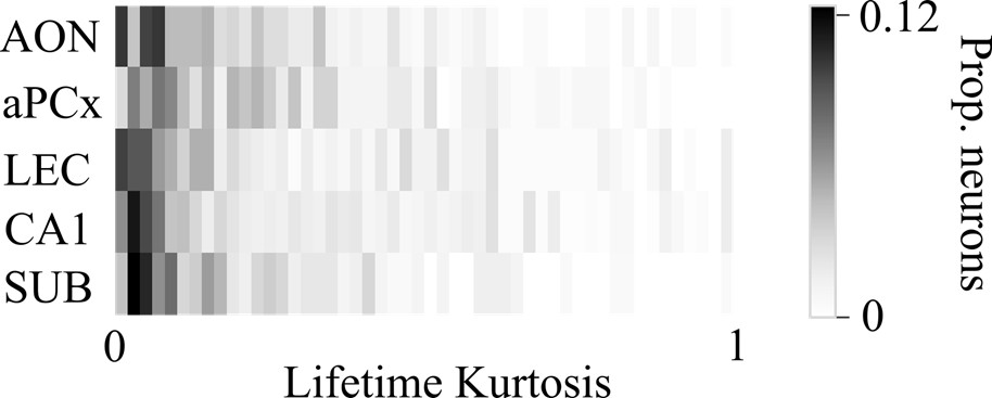
(11) From the model and text, one predicts that the lifetime sparseness increases along the pathway. The authors should use this metric as well/instead of "odor selectivity" because of problems with arbitrary thresholding.
We acknowledge that lifetime sparseness, often computed using lifetime kurtosis, can be an informative measure of selectivity. However, we believe it has limitations that make it less suitable for our analysis. One key issue is that lifetime sparseness does not account for the stability of responses across multiple presentations of the same stimulus. In contrast, our odor selectivity measure incorporates trial-to-trial variability by considering responses over 10 trials and assessing significance using a Wilcoxon test compared to baseline. While the choice of a p-value threshold (e.g., 0.05) is somewhat arbitrary, it is a widely accepted statistical convention. Additionally, lifetime sparseness does not account for excitatory and inhibitory responses. For example, if a neuron X is strongly inhibited by odor A, strongly excited by odor B, and unresponsive to odors C and D, lifetime sparseness would classify it as highly selective for odor B, without capturing its inhibitory selectivity for odor A. The lifetime sparseness will be higher than if X was simply unresponsive for A.
Our odor selectivity measure addresses this by considering both excitation and inhibition as potential responses. Thus, while lifetime sparseness could provide a useful complementary perspective in another type of dataset, it does not fully capture the dynamics of odor selectivity here.
Author response 1.
Lifetime Kurtosis distribution per region.
Reviewer #3 (Recommendations for the authors):
Main points:
(1) The authors use a non-associative learning paradigm - repeated odor exposure - to test how experience modulates odor responses along the olfactory-hippocampal pathway. While repeated odor exposure clearly modulates odor-evoked neural activity, the relevance of this modulation and its differential effect across different brain areas are difficult to assess in the absence of any behavioral read-outs.
Our experimental paradigm involves a robust, reliable behavioral readout of non-associative learning. Novel olfactory stimuli evoke a well-characterized orienting reaction, which includes a multitude of physiological reactions, including exploratory sniffing, facial movements and pupil dilation (Modirshanechi et al., Trends Neuroscience 2023). In our study, we focused on exploration sniffing.
Compared to associative learning, non-associative learning might have received less attention. However, it is critically important because it forms the foundation for how organisms adapt to their environment through experience without forming associations. This is highlighted by the fact that non-instrumental stimuli can be remembered in large number (Standing, 1973) and with remarkable detail (Brady et al., 2008). While non-associative learning can thus create vast, implicit memory of stimuli in the environment, it is unclear how stimulus representations reflect this memory. Our study contributes to answering this question. We describe the impact of experience on olfactory sensory representations and reveal a transformation of representations from olfactory cortical to hippocampal structures. Our findings also indicate that sensory responses to familiar stimuli persist within sensory cortical and hippocampal regions, even after spontaneous orienting behaviors habituated. Further studies involving experimental manipulation techniques are needed to elucidate the causal mechanisms underlying the formation of stimulus memory during non-associative learning.
(2) The authors discuss the olfactory-hippocampal pathway as a transition from primary sensory (AON, aPCx) to associative areas (LEC, CA1, SUB). While this is reasonable, given the known circuit connectivity, other interpretations are possible. For example, AON, aPCx, and LEC receive direct inputs from the olfactory bulb ('primary cortex'), while CA1 and SUB do not; AON receives direct top-down inputs from CA1 ('associative cortex'), while aPCx does not. In fact, the data presented in this manuscript does not appear to support a consistent, smooth transformation from sensory to associative, as implied by the authors (e.g. Figure 4A, F, and G).
Thank you for this insightful comment. Indeed, there are complexities in the circuitry, and the relationships between different areas are not linear. We believe that AON and aPCx are distinctly different from LEC, CA1 and SUB, as the latter areas have been shown to integrate multimodal sensory information. To avoid confusion due to definitions of what constitutes a “primary sensory” region, we adopted a more neutral description throughout the manuscript. We also removed the term “gradual” to describe the transition of neural representations from olfactory cortical to hippocampal areas.
(3) The analysis of odor-evoked responses is focused on a 400 ms window to exclude differences in sniffing behavior. This window spans 200 ms before and after the first inhalation after odor onset. Inhalation onset initiates neural odor responses - why do the authors include neural data before inhalation onset?
The reason to include a brief time window prior to odor onset is to account for what is often called “partical” sniffs. In our experimental setup, odor delivery is not triggered by the animal’s inhalation. Therefore, it can happen that an animal has just begun to inhale when the stimulus is delivered. In this case, the animal is exposed to odorant molecules prior to the first complete inhalation after odor onset. We acknowledge that this limits the temporal resolution of our measurements, but it does not affect the comparison of sensory representations between different brain areas.
It would also be interesting to explore the effect of sniffing behavior (see point 2) on odor-evoked neural activity.
Thank you for your comment, we performed additional analysis including a GLM to address this question (Figure S2C-D).
Minor points:
(4) Figure 2A represents raster plots for 2 neurons per area - it is unclear how to distinguish between the 2 neurons in the plots.
Figure 2A shows one example neuron per brain area. Each neurons has two raster plot which indicate responses to either a novel (orange) or a familiar stimulus (blue). We have revised the figure caption for clarity.
(5) Overall, axes should be kept consistent and labeled in more detail. For example, Figure 2H and I are difficult to compare, given that the y-axis changes and that decoding accuracies are difficult to estimate without additional marks on the y-axis.
Axes are indeed different, because chance level decoding accuracy is different between those two figures. The decoding between novel and familiar odors has a chance level of 0.5, while chance level decoding odors is 0.1 (there are 10 odors to decode the identity from).
(6) Some parts of the discussion seem only loosely related to the data presented in this manuscript. For example, the statement that 'AON rather than aPCx should be considered as the primary sensory cortex in olfaction' seems out of context. Similarly, it would be helpful to provide data on the stability of subpopulations of neurons tuned to familiar odors, rather than simply speculate that they could be stable. The authors could summarize more speculative statements in an 'Ideas and Speculation' subsection.
Thank you for your comment. We appreciate your perspective on our hypotheses. We have revised the discussion accordingly. Specifically, we removed the discussion of stable subpopulations, since we have not performed longitudinal tracking in this study.
(7) The authors should try to reference relevant published work more comprehensively.
Thank you for your comment. We attempted to include relevant published work without exceeding the limit for references but might have overseen important contributions. We apologize to our colleagues, whose relevant work might not have been cited.
Author response:
The following is the authors’ response to the original reviews.
Public Reviews:
Reviewer #1 (Public review):
Summary:
The main contributions of this paper are: (1) a replication of the surprising prior finding that information about peripherally-presented stimuli can be decoded from foveal V1 (Williams et al 2008), (2) a new demonstration of cross-decoding between stimuli presented in the periphery and stimuli presented at the fovea, (3) a demonstration that the information present in the fovea is based on shape not semantic category, and (4) a demonstration that the strength of foveal information about peripheral targets is correlated with the univariate response in the same block in IPS.
Strengths:
The design and methods appear sound, and finding (2) above is new, and importantly constrains our understanding of this surprising phenomenon. The basic effect investigated here is so surprising that even though it has been replicated several times since it was first reported in 2008, it is useful to replicate it again.
We thank the reviewer for their summary. While we agree with many points, we would like to respectfully push back on the notion that this work is a replication of Williams et al. (2008). What our findings share with those of Williams is a report of surprising decoding at the fovea without foveal stimulation. Beyond this similarity, we treat these as related but clearly separate findings, for the following reasons:
(1) Foveal feedback, as shown by Williams et al. (2008) and others during fixation, was only observed during a shape discrimination task, specific to the presented stimulus. Control experiments without such a task (or a color-related task) did not show effects of foveal feedback. In contrast, in the present study, the participants’ task was merely to perform saccades towards stimuli, independently of target features. We thus show that foveal feedback can occur independently of a task related to stimulus features. This dissociation demonstrates that our study must be tapping into something different than reported by Williams.
(2) In a related study, Kroell and Rolfs (2022, 2025) demonstrated a connection between foveal feedback and saccade preparation, including the temporal details of the onset of this effect before saccade execution, highlighting the close link of this effect to saccade preparation. Here we used a very similar behavioral task to capture this saccade-related effect in neural recordings and investigate how early it occurs and what its nature is. Thus, there is a clear motivation for this study in the context of eye movement preparation that is separate from the previous work by Williams.
(3) Lastly, decoding in the experimental task was positively associated with activity in FEF and IPS, areas that have been reliably linked to saccade preparation. We have now also performed an additional analysis (see our response to Specific point 2 of Reviewer 2) showing that decoding in the control condition did not show the same association, further supporting the link of foveal feedback to saccade preparation.
Despite our emphasis on these critical differences in studies, covert peripheral attention, as required by the task in Williams et al., and saccade preparation in natural vision, as in our study, are tightly coupled processes. Indeed, the task in Williams et al. would, during natural vision, likely involve an eye movement to the peripheral target. While speculative, a parsimonious and ecologically valid explanation is that both ours and earlier studies involve eye movement preparation, for which execution is suppressed, however, in studies enforcing fixation (e.g., Williams et al., 2008). We now discuss this idea of a shared underlying mechanism more extensively in the revised manuscript (pg 8 ln 228-240).
Weaknesses:
(1) The paper, including in the title ("Feedback of peripheral saccade targets to early foveal cortex") seems to assume that the feedback to foveal cortex occurs in conjunction with saccade preparation. However, participants in the original Williams et al (2008) paper never made saccades to the peripheral stimuli. So, saccade preparation is not necessary for this effect to occur. Some acknowledgement and discussion of this prior evidence against the interpretation of the effect as due to saccade preparation would be useful. (e.g., one might argue that saccade preparation is automatic when attending to peripheral stimuli.)
We agree that the effects Williams et al. showed were not sufficiently discussed in the first version of this manuscript. To more clearly engage with these findings we now introduce saccade related foveal feedback (foveal prediction) and foveal feedback during fixation separately in the introduction (pg 2 ln 46-59).
We further added another section in the discussion called “Foveal feedback during saccade preparation” in which we discuss how our findings are related to Williams et al. and how they differ (pg 8 ln 211-240).
As described in our previous response, we believe that our findings go beyond those described by Williams et al. (2008) and others in significant ways. However, during natural vision, the paradigm used by Williams et al. (2008) would likely be solved using an eye movement. Thus, while participants in Williams et al. (2008) did not execute saccades, it appears plausible that they have prepared saccades. Given the fact that covert peripheral attention and saccade preparation are tightly coupled processes (Kowler et al., 1995, Vis Res; Deubel & Schneider, 1996, Vis Res; Montagnini & Castet, 2007, J Vis; Rolfs & Carrasco, 2012, J Neurosci; Rolfs et al., 2011, Nat Neurosci), their results are parsimoniously explained by saccade preparation (but not execution) to a behaviorally relevant target.
(2) The most important new finding from this paper is the cross-decodability between stimuli presented in the fovea and stimuli presented in the periphery. This finding should be related to the prior behavioral finding (Yu & Shim, 2016) that when a foveal foil stimulus identical to a peripheral target is presented 150 ms after the onset of the peripheral target, visual discrimination of the peripheral target is improved, and this congruency effect occurred even though participants did not consciously perceive the foveal stimulus (Yu, Q., & Shim, W. M., 2016). Modulating foveal representation can influence visual discrimination in the periphery (Journal of Vision, 16(3), 15-15).
We thank the reviewer for highlighting this highly relevant reference. In the revised version of the manuscript, we now put more emphasis on the finding of cross-decodability (pg 2 ln 60-61). We now also discuss Yu et al.’s finding, which support our conclusion that foveal feedback and direct stimulus presentation share representational formats in early visual areas (pg 9 ln 277-279).
(3) The prior literature should be laid out more clearly. For example, most readers will not realize that the basic effect of decodability of peripherally-presented stimuli in the fovea was first reported in 2008, and that that original paper already showed that the effect cannot arise from spillover effects from peripheral retinotopic cortex because it was not present in a retinotopic location between the cortical locus corresponding to the peripheral target and the fovea. (For example, this claim on lines 56-57 is not correct: "it remains unknown 1) whether information is fed back all the way to early visual areas".) What is needed is a clear presentation of the prior findings in one place in the introduction to the paper, followed by an articulation and motivation of the new questions addressed in this paper. If I were writing the paper, I would focus on the cross-decodability between foveal and peripheral stimuli, as I think that is the most revealing finding.
We agree that the structure of the introduction did not sufficiently place our work in the context of prior literature. We have now expanded upon our Introduction section to discuss past studies of saccade- and fixation-related foveal feedback (pg 2 ln 49-59), laying out how this effect has been studied previously. We also removed the claim that "it remains unknown 1) whether information is fed back all the way to early visual areas", where our intention was to specifically focus on foveal prediction. We realize that this was not clear and hence removed this section. Instead, we now place a stronger focus on the cross-decodability finding (pg 2 ln 60-61).
Reviewer #2 (Public review):
Summary:
This study investigated whether the identity of a peripheral saccade target object is predictively fed back to the foveal retinotopic cortex during saccade preparation, a critical prediction of the foveal prediction hypothesis proposed by Kroell & Rolfs (2022). To achieve this, the authors leveraged a gaze-contingent fMRI paradigm, where the peripheral saccade target was removed before the eyes landed near it, and used multivariate decoding analysis to quantify identity information in the foveal cortex. The results showed that the identity of the saccade target object can be decoded based on foveal cortex activity, despite the fovea never directly viewing the object, and that the foveal feedback representation was similar to passive viewing and not explained by spillover effects. Additionally, exploratory analysis suggested IPS as a candidate region mediating such foveal decodability. Overall, these findings provide neural evidence for the foveal cortex processing the features of the saccade target object, potentially supporting the maintenance of perceptual stability across saccadic eye movements.
Strengths:
This study is well-motivated by previous theoretical findings (Kroell & Rolfs, 2022), aiming to provide neural evidence for a potential neural mechanism of trans-saccadic perceptual stability. The question is important, and the gaze-contingent fMRI paradigm is a solid methodological choice for the research goal. The use of stimuli allowing orthogonal decoding of stimulus category vs stimulus shape is a nice strength, and the resulting distinctions in decoded information by brain region are clean. The results will be of interest to readers in the field, and they fill in some untested questions regarding pre-saccadic remapping and foveal feedback.
We thank the reviewer for the positive assessment of our study.
Weaknesses:
The conclusions feel a bit over-reaching; some strong theoretical claims are not fully supported, and the framing of prior literature is currently too narrow. A critical weakness lies in the inability to test a distinction between these findings (claiming to demonstrate that "feedback during saccade preparation must underlie this effect") and foveal feedback previously found during passive fixation (Williams et al., 2008). Discussions (and perhaps control analysis/experiments) about how these findings are specific to the saccade target and the temporal constraints on these effects are lacking. The relationship between the concepts of foveal prediction, foveal feedback, and predictive remapping needs more thorough treatment. The choice to use only 4 stimuli is justified in the manuscript, but remains an important limitation. The IPS results are intriguing but could be strengthened by additional control analysis. Finally, the manuscript claims the study was pre-registered ("detailing the hypotheses, methodology, and planned analyses prior to data collection"), but on the OSF link provided, there is just a brief summary paragraph, and the website says "there have been no completed registrations of this project".
We thank the reviewer for these helpful considerations. We agree that some of the claims were not sufficiently supported by the evidence, and in the revised manuscript, we added nuance to those claims (pg 8 ln 211-240). Furthermore, we now address more directly the distinction between foveal feedback during fixation and foveal feedback (foveal prediction) during saccade preparation. In particular, we now describe the literature about these two effects separately in the introduction (pg 2 ln 46-59), and we have added a new section in the discussion (“Foveal feedback during saccade preparation”) that more thoroughly explains why a passive fixation condition would have been unlikely to produce the same results we find (pg 8 ln 211-227). We also adapted the section about “Saccadic remapping or foveal prediction”, clearly delineating foveal prediction from feature remapping and predictive updating of attention pointers. As recommended by the reviewer, we conducted the parametric modulation analyses on the control condition, strengthening the claim that our findings are saccade-related. These results were added as Supplementary Figure 2 and are discussed in (pg 7 ln 190-191) and (pg 8 ln 224-227).
Lastly, we would like to apologize about a mistake we made with the pre-registration. We realized that the pre-registration had indeed not been submitted. We have now done so without changing the pre-registration itself, which can be seen from the recent activity of the preregistration (screenshot attached in the end). After consulting an open science expert at the University of Leipzig, we added a note of this mistake to the methods section of the revised manuscript (pg 10 ln 326-332). We could remove reference to this preregistration altogether, but would keep it at the discretion of the editor.
Specifics:
(1) In the eccentricity-dependent decoding results (Figure 2B), are there any statistical tests to support the results being a U-shaped curve? The dip isn't especially pronounced. Is 4 degrees lower than the further ones? Are there alternative methods of quantifying this (e.g., fitting it to a linear and quadratic function)?
We statistically tested the U-shaped relationship using a weighted quadratic regression, which showed significant positive curvature for decoding between fovea and periphery in all early visual areas (V1: t(27) = 3.98, p = 0.008, V2: t(27) = 3.03, p = 0.02, V3: t(27)= 2.776, p = 0.025, one-sided). We now report these results in the revised manuscript (pg 5 ln 137-138).
(2) In the parametric modulation analysis, the evidence for IPS being the only region showing stronger fovea vs peripheral beta values was weak, especially given the exploratory nature of this analysis. The raw beta value can reflect other things, such as global brain fluctuations or signal-to-noise ratio. I would also want to see the results of the same analysis performed on the control condition decoding results.
We appreciate the reviewer’s suggestion and repeated the same parametric modulation analysis on the control condition to assess the influence of potential confounds on the overall beta values (Supplementary Figure 2). The results show a negative association between foveal decoding and FEF and IPS (likely because eye movements in the control condition lead to less foveal presentation of the stimulus) and a positive association with LO. Peripheral decoding was not associated with significant changes in any of the ROIs, indicating that global brain fluctuations alone are not responsible for the effects reported in the experimental condition. The results of this analysis thus show a specific positive association of IPS activity with the experimental condition, not the control condition, which is in line with the idea that the foveal feedback effect reported in this study may be related to saccade preparation.
(3) Many of the claims feel overstated. There is an emphasis throughout the manuscript (including claims in the abstract) that these findings demonstrate foveal prediction, specifically that "image-specific feedback during saccade preparation must underlie this effect." To my understanding, one of the key aspects of the foveal prediction phenomenon that ties it closely to trans-saccadic stability is its specificity to the saccade target but not to other objects in the environment. However, it is not clear to what degree the observed findings are specific to saccade preparation and the peripheral saccade target. Should the observers be asked to make a saccade to another fixation location, or simply maintain passive fixation, will foveal retinotopic cortex similarly contain the object's identity information? Without these control conditions, the results are consistent with foveal prediction, but do not definitively demonstrate that as the cause, so claims need to be toned down.
We fully agree with the reviewer and toned down claims about foveal prediction. We engage with the questions raised by the reviewer more thoroughly in the new discussion section “Foveal feedback during saccade preparation”.
In addition, we agree that another condition in which subjects make a saccade towards a different location would have been a great addition that we also considered, but due to concerns with statistical power did not add. While including such a condition exceeds the scope of the current study, we included this limitation in the Discussion section (pg 10 ln 316) and hope that future studies will address this question.
(4) Another critical aspect is the temporal locus of the feedback signal. In the paradigm, the authors ensured that the saccade target object was never foveated via the gaze-contingent procedure and a conservative data exclusion criterion, thus enabling the test of feedback signals to foveal retinotopic cortex. However, due to the temporal sluggishness of fMRI BOLD signals, it is unclear when the feedback signal arrives at the foveal retinotopic cortex. In other words, it is possible that the feedback signal arrives after the eyes land at the saccade target location. This possibility is also bolstered by Chambers et al. (2013)'s TMS study, where they found that TMS to the foveal cortex at 350-400 ms SOA interrupts the peripheral discrimination task. The authors should qualify their claims of the results occurring "during saccade preparation" (e.g., pg 1 ln 22) throughout the manuscript, and discuss the importance of temporal dynamics of the effect in supporting stability across saccades.
We fully agree that the sluggishness of the fMRI signal presents an important challenge in investigating foveal feedback. We have now included this limitation in the discussion (pg 10 ln 306-318). We also clarify that our argument connects to previous studies investigating the temporal dynamics of foveal feedback using similar tasks (pg 10 ln 313-316). Specifically, in their psychophysical work, Kroell and Rolfs (2022) and (2025) showed that foveal feedback occurs before saccade execution with a peak around 80 ms before the eye movement.
(5) Relatedly, the claims that result in this paradigm reflect "activity exclusively related to predictive feedback" and "must originate from predictive rather than direct visual processes" (e.g., lines 60-65 and throughout) need to be toned down. The experimental design nicely rules out direct visual foveal stimulation, but predictive feedback is not the only alternative to that. The activation could also reflect mental imagery, visual working memory, attention, etc. Importantly, the experiment uses a block design, where the same exact image is presented multiple times over the block, and the activation is taken for the block as a whole. Thus, while at no point was the image presented at the fovea, there could still be more going on than temporally-specific and saccade-specific predictive feedback.
We agree that those claims could have misled the reader. Our intention was to state that the activation originates from feedback rather than direct foveal stimulation because of the nature of the design. We have now clarified these statements (pg 2 ln 65) and also included a discussion of other effects including imagery and working memory in the limitations section (pg 10 ln 306-313).
(6) The authors should avoid using the terms foveal feedback and foveal prediction interchangeably. To me, foveal feedback refers to the findings of Williams et al. (2008), where participants maintained passive fixation and discriminated objects in the periphery (see also Fan et al., 2016), whereas foveal prediction refers to the neural mechanism hypothesized by Kroell & Rolfs (2022), occurring before a saccade to the target object and contains task irrelevant feature information.
We agree, and we have now adopted a clearer distinction between these terms, referring to foveal prediction only when discussing the distinct predictive nature of the effect discovered by Kroell and Rolfs (2022). Otherwise we referred to this effect as foveal feedback.
(7) More broadly, the treatment of how foveal prediction relates to saccadic remapping is overly simplistic. The authors seem to be taking the perspective that remapping is an attentional phenomenon marked by remapping of only attentional/spatial pointers, but this is not the classic or widely accepted definition of remapping. Within the field of saccadic remapping, it is an ongoing debate whether (/how/where/when) information about stimulus content is remapped alongside spatial location (and also whether the attentional pointer concept is even neurophysiologically viable). This relationship between saccadic remapping and foveal prediction needs clarification and deeper treatment, in both the introduction and discussion.
We thank the reviewer for their remarks. We reformulated the discussion section on “Saccadic remapping or foveal prediction” to include the nuances about spatial and feature remapping laid out in the reviewer’s comment (pg 8-9 ln 241-269). We also put a stronger focus on the special role the fovea seems to be playing regarding the feedback of visual features (pg 8-9 ln 265-269).
(8) As part of this enhanced discussion, the findings should be better integrated with prior studies. E.g., there is some evidence for predictive remapping inducing integration of non-spatial features (some by the authors themselves; Harrison et al., 2013; Szinte et al., 2015). How do these findings relate to the observed results? Can the results simply be a special case of non-spatial feature integration between the currently attended and remapped location (fovea)? How are the results different from neurophysiological evidence for facilitation of the saccade target object's feature across the visual field (Burrow et al., 2014)? How might the results be reconciled with a prior fMRI study that failed to find decoding of stimulus content in remapped responses (Lescroart et al, 2016)? Might this reflect a difference between peripheral-to-peripheral vs peripheral-to-foveal remapping? A recent study by Chiu & Golomb (2025) provided supporting evidence for peripheral-to-fovea remapping (but not peripheral-to-peripheral remapping) of object-location binding (though in the post-saccadic time window), and suggested foveal prediction as the underlying mechanism.
We thank the reviewer for raising these intriguing questions. We now address them in the revised discussion. We argue that the findings by Harrison et al., 2013 and Szinte et al., 2015 of presaccadic integration of features across two peripheral locations can be explained by presaccadic updating of spatial attention pointers rather than remapping of feature information (pg 8 ln 248-253). The lack of evidence for periphery-to-periphery remapping (Lescroart et al, 2016) and the recent study by Chiu & Golomb (2025) showing object-location binding from periphery to fovea nicely align with our characterization of foveal processing as unique in predicting feature information of upcoming stimuli (pg 8-9 ln 265-269). Finally, we argue that the global (i.e., space-invariant) selection task-irrelevant saccadic target features (Burrows et al., 2014) is well-established at the neural level, but does not suffice to explain the spatially specific nature of foveal prediction (pg 8 ln 220-224). We now include these studies in the revised discussion section.
Reviewer #3 (Public review):
Summary:
In this paper, the authors used fMRI to determine whether peripherally viewed objects could be decoded from the foveal cortex, even when the objects themselves were never viewed foveally. Specifically, they investigated whether pre-saccadic target attributes (shape, semantic category) could be decoded from the foveal cortex. They found that object shape, but not semantic category, could be decoded, providing evidence that foveal feedback relies on low-mid-level information. The authors claim that this provides evidence for a mechanism underlying visual stability and object recognition across saccades.
Strengths:
I think this is another nice demonstration that peripheral information can be decoded from / is processed in the foveal cortex - the methods seem appropriate, and the experiments and analyses are carefully conducted, and the main results seem convincing. The paper itself was very clear and well-written.
We thank the reviewer for this positive evaluation of our work. As discussed in our response to Reviewer 1, we now elaborate on the differences between previous work showing decoding of peripheral information from foveal cortex from the effect shown here. While there are important similarities between these findings, foveal prediction in our study occurs in a saccade condition and in the absence of a task that is specific to stimulus features.
Weaknesses:
There are a couple of reasons why I think the main theoretical conclusions drawn from the study might not be supported, and why a more thorough investigation might be needed to draw these conclusions.
(1) The authors used a blocked design, with each object being shown repeatedly in the same block. This meant that the stimulus was entirely predictable on each block, which weakens the authors' claims about this being a predictive mechanism that facilitates object recognition - if the stimulus is 100% predictable, there is no aspect of recognition or discrimination actually being tested. I think to strengthen these claims, an experiment would need to have unpredictable stimuli, and potentially combine behavioural reports with decoding to see whether this mechanism can be linked to facilitating object recognition across saccades.
We appreciate the reviewer’s point and would like to highlight that it was not our intention to claim a behavioral effect on object recognition. We believe that an ambiguous formulation in the original abstract may have been interpreted this way, and we thus removed this reference. We also speculated in our Discussion that a potential reason for foveal prediction could be a headstart in peripheral object recognition and in the revised manuscript more clearly highlight that this is a potential future direction only.
(2) Given that foveal feedback has been found in previous studies that don't incorporate saccades, how is this a mechanism that might specifically contribute to stability across saccades, rather than just being a general mechanism that aids the processing/discrimination of peripherally-viewed stimuli? I don't think this paper addresses this point, which would seem to be crucial to differentiate the results from those of previous studies.
We fully agree that this point had not been sufficiently addressed in the previous version of the manuscript. As described in our responses to similar comments from reviewers 1 and 2, we included an additional section in the Discussion (“Foveal feedback during saccade preparation”) to more clearly delineate the present study from previous findings of foveal feedback. Previous studies (Williams et al., 2008) only found foveal feedback during narrow discrimination tasks related to spatial features of the target stimulus, not during color-discrimination or fixation-only tasks, concluding that the observed effect must be related to the discrimination behavior. In contrast, we found foveal feedback (as evidenced by decoding of target features) during a saccade condition that was independent of the target features, suggesting a different role of foveal feedback than hypothesized by Williams et al. (2008).
Recommendations for the authors:
Reviewer #2 (Recommendations for the authors):
(A) Minor comments:
(1) The task should be clarified earlier in the manuscript.
We now characterise the task in the abstract and clarified its description in the third paragraph, right after introducing the main literature.
(2) Is there actually only 0.5 seconds between saccades? This feels very short/rushed.
The inter-trial-interval was 0.5 seconds, though effectively it varied because the target only appeared once participants fixated on the fixation dot. Note that this pacing is slower than the rate of saccades in natural vision (about 3 to 4 saccades per second).Participants did not report this paradigm as rushed.
(3) Typo on pg2 ln64 (whooe).
Fixed.
(4) Can the authors also show individual data points for Figures 3 and 4?
We added individual data points for Figures 4 and S2
(5) The MNI coordinates on Figure 4A seem to be incorrect.
We took out those coordinates.
(6) Pg4 ln126 and pg6 ln194, why cite Williams et al. (2008)?
We included this reference here to acknowledge that Williams et al. raised the same issues. We added a “cf.” before this reference to clarify this.
(7) Pg7 ln207 Fabius et al. (2020) showed slow post-saccadic feature remapping, rather than predictive remapping of spatial attention.
We have corrected this mistake.
(8) The OSF link is valid, but I couldn't find a pre-registration.
The issue with the OSF link has been resolved. The pre-registration had been set up but not published. We now published it without changing the original pre-registration (see the screenshot attached).
(9) I couldn't access the OpenNeuro repository.
The issue with the OpenNeuro link has been resolved.
(B) Additional references you may wish to include:
(1) Burrows, B. E., Zirnsak, M., Akhlaghpour, H., Wang, M., & Moore, T. (2014). Global selection of saccadic target features by neurons in area v4. Journal of Neuroscience.
(2) Chambers, C. D., Allen, C. P., Maizey, L., & Williams, M. A. (2013). Is delayed foveal feedback critical for extra-foveal perception?. Cortex.
(3) Chiu, T. Y., & Golomb, J. D. (2025). The influence of saccade target status on the reference frame of object-location binding. Journal of Experimental Psychology. General.
(4) Harrison, W. J., Retell, J. D., Remington, R. W., & Mattingley, J. B. (2013). Visual crowding at a distance during predictive remapping. Current Biology.
(5) Lescroart, M. D., Kanwisher, N., & Golomb, J. D. (2016). No evidence for automatic remapping of stimulus features or location found with fMRI. Frontiers in Systems Neuroscience.
(6) Moran, C., Johnson, P. A., Hogendoorn, H., & Landau, A. N. (2025). The representation of stimulus features during stable fixation and active vision. Journal of Neuroscience.
(7) Szinte, M., Jonikaitis, D., Rolfs, M., Cavanagh, P., & Deubel, H. (2016). Presaccadic motion integration between current and future retinotopic locations of attended objects. Journal of Neurophysiology.
We thank the reviewer for pointing out these references. We have included them in the revised version of the manuscript.
Reviewer #3 (Recommendations for the authors):
I just have a few minor points where I think some clarifications could be made.
(1) Line 64 - "whooe" should be "whoose" I think.
Fixed.
(2) Around line 53 - you might consider citing this review on foveal feedback - https://doi.org/10.1167/jov.20.12.2
We included the reference (pg 2 ln 55).
(3) Line 129 - you mention a u-shaped relationship for decoding - I wasn't quite sure of the significance/relevance of this relationship - it would be helpful to expand on this / clarify what this means.
We have expanded this section and added statistical tests of the u-shaped relationship in decoding using a weighted quadratic regression. We found significant positive curvature in all early visual areas between fovea and periphery (V1: t(27) = 3.98, p = 0.008, V2: t(27) = 3.03, p = 0.02, V3: t(27)= 2.776, p = 0.025). These findings support a u-shaped relationship. We now report these results in the revised manuscript (pg 5 ln 137-138).
(4) Figure 1 - it would be helpful to indicate how long the target was viewed in the "stim on" panels - I assume it was for the saccade latency, but it would be good to include those values in the main text.
We included that detail in the text (pg 3 ln 96-97).
Author response:
The following is the authors’ response to the current reviews.
Public Reviews:
Reviewer #1 (Public review):
Summary:
This study examines whether changes in pupil size index prediction-error-related updating during associative learning, formalised as information gain via Kullback-Leibler (KL) divergence. Across two independent tasks, pupil responses scaled with KL divergence shortly after feedback, with the timing and direction of the response varying by task. Overall, the work supports the view that pupil size reflects information-theoretic processes in a context-dependent manner.
Strengths:
This study provides a novel and convincing contribution by linking pupil dilation to informationtheoretic measures, such as KL divergence, supporting Zénon's hypothesis that pupil responses reflect information gain during learning. The robust methodology, including two independent datasets with distinct task structures, enhances the reliability and generalisability of the findings. By carefully analysing early and late time windows, the authors capture the timing and direction of prediction-error-related responses, oPering new insights into the temporal dynamics of model updating. The use of an ideal-learner framework to quantify prediction errors, surprise, and uncertainty provides a principled account of the computational processes underlying pupil responses. The work also highlights the critical role of task context in shaping the direction and magnitude of these ePects, revealing the adaptability of predictive processing mechanisms. Importantly, the conclusions are supported by rigorous control analyses and preprocessing sanity checks, as well as convergent results from frequentist and Bayesian linear mixed-ePects modelling approaches.
Weaknesses:
Some aspects of directionality remain context-dependent, and on current evidence cannot be attributed specifically to whether average uncertainty increases or decreases across trials. DiPerences between the two tasks (e.g., sensory modality and learning regime) limit direct comparisons of ePect direction and make mechanistic attribution cautious. In addition, subjective factors such as confidence were not measured and could influence both predictionerror signals and pupil responses. Importantly, the authors explicitly acknowledge these limitations, and the manuscript clearly frames them as areas for future work rather than settled conclusions.
Reviewer #2 (Public review):
Summary:
The authors investigate whether pupil dilation reflects information gain during associative learning, formalised as Kullback-Leibler divergence within an ideal observer framework. They examine pupil responses in a late time window after feedback and compare these to informationtheoretic estimates (information gain, surprise, and entropy) derived from two diPerent tasks with contrasting uncertainty dynamics.
Strength:
The exploration of task evoked pupil dynamics beyond the immediate response/feedback period and then associating them with model estimates was interesting and inspiring. This oPered a new perspective on the relationship between pupil dilation and information processing.
Weakness:
However, the interpretability of the findings remains constrained by the fundamental diPerences between the two tasks (stimulus modality, feedback type, and learning structure), which confound the claimed context-dependent ePects. The later time-window pupil ePects, although intriguing, are small in magnitude and may reflect residual noise or task-specific arousal fluctuations rather than distinct information-processing signals. Thus, while the study oPers valuable methodological insight and contributes to ongoing debates about the role of the pupil in cognitive inference, its conclusions about the functional significance of late pupil responses should be treated with caution.
Reviewer #3 (Public review):
Summary:
Thank you for inviting me to review this manuscript entitled "Pupil dilation oPers a time-window on prediction error" by Colizoli and colleagues. The study examines prediction errors, information gain (Kullback-Leibler [KL] divergence), and uncertainty (entropy) from an information-theory perspective using two experimental tasks and pupillometry. The authors aim to test a theoretical proposal by Zénon (2019) that the pupil response reflects information gain (KL divergence). The conclusion of this work is that (post-feedback) pupil dilation in response to information gain is context dependent.
Strengths:
Use of an established Bayesian model to compute KL divergence and entropy.
Pupillometry data preprocessing and multiple robustness checks.
Weaknesses:
Operationalization of prediction errors based on frequency, accuracy, and their interaction:
The authors rely on a more model-agnostic definition of the prediction error in terms of stimulus frequency ("unsigned prediction error"), accuracy, and their interaction ("signed prediction error"). While I see the point, I would argue that this approach provides a simple approximation of the prediction error, but that a model-based approach would be more appropriate.
Model validation:
My impression is that the ideal learner model should work well in this case. However, the authors don't directly compare model behavior to participant behavior ("posterior predictive checks") to validate the model. Therefore, it is currently unclear if the model-derived terms like KL divergence and entropy provide reasonable estimates for the participant data.
Lack of a clear conclusion:
The authors conclude that this study shows for the first time that (post-feedback) pupil dilation in response to information gain is context dependent. However, the study does not oPer a unifying explanation for such context dependence. The discussion is quite detailed with respect to taskspecific ePects, but fails to provide an overarching perspective on the context-dependent nature of pupil signatures of information gain. This seems to be partly due to the strong diPerences between the experimental tasks.
Recommendations for the authors:
Reviewer #1 (Recommendations for the authors):
I highly appreciate the care and detail in the authors' response and thank them for the ePort invested in revising the manuscript. They addressed the core concerns to a high standard, and the manuscript has substantially improved in methodological rigour (through additional controls/sanity checks and complementary mixed-ePects analyses) and in clarity of interpretation (by explicitly acknowledging context-dependence and tempering stronger claims). The present version reads clearly and is much strengthened overall. I only have a few minor points below:
Minor suggestions:
Abstract:
In the abstract KL is introduced as abbreviation, but at first occurence it should be written out as "Kullback-Leibler (KL)" for readers not familiar with it.
We thank the reviewer for catching this error. It has been correct in the version of record.
Methods:
I appreciate the additional bayesian LME analysis. I only had a few things that I thought were missing from knowing the parameters: 1) what was the target acceptance rate (default of .95?), 2) which family was used to model the response distribution: (default) "gaussian" or robust "student-t"? Depending on the data a student-t would be preferred, but since the author's checked the fit & the results corroborate the correlation analysis, using the default would also be fine! Just add the information for completeness.
Thank you for bringing this to our attention. We have now noted that default parameters were used in all cases unless otherwise mentioned.
Thank you once again for your time and consideration.
Reviewer #2 (Recommendations for the authors):
Thanks to the authors' ePort on revision. I am happy with this new version of manuscript.
Thank you once again for your time and consideration.
Reviewer #3 (Recommendations for the authors):
(1) Regarding comments #3 and #6 (first round) on model validation and posterior predictive checks, the authors replied that since their model is not a "generative" one, they can't perform posterior predictive checks. Crucially, in eq. 2, the authors present the p{tilde}^j_k variable denoting the learned probability of event k on trial j. I don't see why this can't be exploited for simulations. In my opinion, one could (and should) generate predictions based on this variable. The simplest implementation would translate the probability into a categorical choice (w/o fitting any free parameter). Based on this, they could assess whether the model and data are comparable.
We thank the reviewer for this clarification. The reviewer suggests using the probability distributions at each trial to predict which event should be chosen on each trial. More specifically, the event(s) with the highest probability on trial j could be used to generate a prediction for the choice of the participant on trial j. We agree that this would indeed be an interesting analysis. However, the response options of each task are limited to two-alternatives. In the cue-target task, four events are modeled (representing all possible cue-target conditions) while the participants’ response options are only “left” and “right”. Similarly, in the letter-color task, 36 events are modeled while the participants’ response options are “match” and “no-match”. In other words, we do not know which event (either four or 36, for the two tasks) the participant would have indicated on each trial. As an approximation to this fine-grained analysis, we investigated the relationship between the information-theoretic variables separately for error and correct trials. Our rationale was that we would have more insight into how the model fits depended on the participants’ actual behavior as compared with the ideal learner model.
(2) I recommend providing a plot of the linear mixed model analysis of the pupil data. Currently, results are only presented in the text and tables, but a figure would be much more useful.
We thank the reviewer for the suggestion to add a plot of the linear mixed model results. We appreciate the value of visualizing model estimates; however, we feel that the current presentation in the text and tables clearly conveys the relevant findings. For this reason, and to avoid further lengthening the manuscript, we prefer to retain the current format.
(3) I would consider only presenting the linear mixed ePects for the pupil data in the main results, and the correlation results in the supplement. It is currently quite long.
We thank the reviewer for this recommendation. We agree that the results section is detailed; however, we consider the correlation analyses to be integral to the interpretation of the pupil data and therefore prefer to keep them in the main text rather than move them to the supplement.
The following is the authors’ response to the original reviews
eLife Assessment
This important study seeks to examine the relationship between pupil size and information gain, showing opposite effects dependent upon whether the average uncertainty increases or decreases across trials. Given the broad implications for learning and perception, the findings will be of broad interest to researchers in cognitive neuroscience, decision-making, and computational modelling. Nevertheless, the evidence in support of the particular conclusion is at present incomplete - the conclusions would be strengthened if the authors could both clarify the differences between model-updating and prediction error in their account and clarify the patterns in the data.
Public Reviews:
Reviewer #1 (Public review):
Summary:
This study investigates whether pupil dilation reflects prediction error signals during associative learning, defined formally by Kullback-Leibler (KL) divergence, an information-theoretic measure of information gain. Two independent tasks with different entropy dynamics (decreasing and increasing uncertainty) were analyzed: the cue-target 2AFC task and the lettercolor 2AFC task. Results revealed that pupil responses scaled with KL divergence shortly after feedback onset, but the direction of this relationship depended on whether uncertainty (entropy) increased or decreased across trials. Furthermore, signed prediction errors (interaction between frequency and accuracy) emerged at different time windows across tasks, suggesting taskspecific temporal components of model updating. Overall, the findings highlight that pupil dilation reflects information-theoretic processes in a complex, context-dependent manner.
Strengths:
This study provides a novel and convincing contribution by linking pupil dilation to informationtheoretic measures, such as KL divergence, supporting Zénon's hypothesis that pupil responses reflect information gained during learning. The robust methodology, including two independent datasets with distinct entropy dynamics, enhances the reliability and generalisability of the findings. By carefully analysing early and late time windows, the authors capture the temporal dynamics of prediction error signals, offering new insights into the timing of model updates. The use of an ideal learner model to quantify prediction errors, surprise, and entropy provides a principled framework for understanding the computational processes underlying pupil responses. Furthermore, the study highlights the critical role of task context - specifically increasing versus decreasing entropy - in shaping the directionality and magnitude of these effects, revealing the adaptability of predictive processing mechanisms.
Weaknesses:
While this study offers important insights, several limitations remain. The two tasks differ significantly in design (e.g., sensory modality and learning type), complicating direct comparisons and limiting the interpretation of differences in pupil dynamics. Importantly, the apparent context-dependent reversal between pupil constriction and dilation in response to feedback raises concerns about how these opposing effects might confound the observed correlations with KL divergence.
We agree with the reviewer’s concerns and acknowledge that the speculation concerning the directional effect of entropy across trials can not be fully substantiated by the current study. As the reviewer points out, the directional relationship between pupil dilation and information gain must be due to other factors, for instance, the sensory modality, learning type, or the reversal between pupil constriction and dilation across the two tasks. Also, we would like to note that ongoing experiments in our lab already contradict our original speculation. In line with the reviewer’s point, we noted these differences in the section on “Limitations and future research” in the Discussion. To better align the manuscript with the above mentioned points, we have made several changes in the Abstract, Introduction and Discussion summarized below:
We have removed the following text from the Abstract and Introduction: “…, specifically related to increasing or decreasing average uncertainty (entropy) across trials.”
We have edited the following text in the Introduction (changes in italics) (p. 5):
“We analyzed two independent datasets featuring distinct associative learning paradigms, one characterized by increasing entropy and the other by decreasing entropy as the tasks progressed. By examining these different tasks, we aimed to identify commonalities (if any) in the results across varying contexts. Additionally, the contrasting directions of entropy in the two tasks enabled us to disentangle the correlation between stimulus-pair frequency and information gain in the postfeedback pupil response.
We have removed the following text from the Discussion:
“…and information gain in fact seems to be driven by increased uncertainty.”
“We speculate that this difference in the direction of scaling between information gain and the pupil response may depend on whether entropy was increasing or decreasing across trials.”
“…which could explain the opposite direction of the relationship between pupil dilation and information gain”
“… and seems to relate to the direction of the entropy as learning progresses (i.e., either increasing or decreasing average uncertainty).”
We have edited the following texts in the Discussion (changes in italics):
“For the first time, we show that the direction of the relationship between postfeedback pupil dilation and information gain (defined as KL divergence) was context dependent.” (p. 29):
Finally, we have added the following correction to the Discussion (p. 30):
“Although it is tempting to speculate that the direction of the relationship between pupil dilation and information gain may be due to either increasing or decreasing entropy as the task progressed, we must refrain from this conclusion. We note that the two tasks differ substantially in terms of design with other confounding variables and therefore cannot be directly compared to one another. We expand on these limitations in the section below (see Limitations and future research).”
Finally, subjective factors such as participants' confidence and internal belief states were not measured, despite their potential influence on prediction errors and pupil responses.
Thank you for the thoughtful comment. We agree with the reviewer that subjective factors, such as participants' confidence, can be important in understanding prediction errors and pupil responses. As per the reviewer’s point, we have included the following limitation in the Discussion (p. 33):
“Finally, while we acknowledge the potential relevance of subjective factors, such as the participants’ overt confidence reports, in understanding prediction errors and pupil responses, the current study focused on the more objective, model-driven measure of information-theoretic variables. This approach aligns with our use of the ideal learner model, which estimates information-theoretic variables while being agnostic about the observer's subjective experience itself. Future research is needed to explore the relationship between information-gain signals in pupil dilation and the observer’s reported experience of or awareness about confidence in their decisions.”
Reviewer #2 (Public review):
Summary:
The authors proposed that variability in post-feedback pupillary responses during the associative learning tasks can be explained by information gain, which is measured as KL divergence. They analysed pupil responses in a later time window (2.5s-3s after feedback onset) and correlated them with information-theory-based estimates from an ideal learner model (i.e., information gain-KL divergence, surprise-subjective probability, and entropy-average uncertainty) in two different associative decision-making tasks.
Strength:
The exploration of task-evoked pupil dynamics beyond the immediate response/feedback period and then associating them with model estimates was interesting and inspiring. This offered a new perspective on the relationship between pupil dilation and information processing.
Weakness:
However, disentangling these later effects from noise needs caution. Noise in pupillometry can arise from variations in stimuli and task engagement, as well as artefacts from earlier pupil dynamics. The increasing variance in the time series of pupillary responses (e.g., as shown in Figure 2D) highlights this concern.
It's also unclear what this complicated association between information gain and pupil dynamics actually means. The complexity of the two different tasks reported made the interpretation more difficult in the present manuscript.
We share the reviewer’s concerns. To make this point come across more clearly, we have added the following text to the Introduction (p. 5):
“The current study was motivated by Zenon’s hypothesis concerning the relationship between pupil dilation and information gain, particularly in light of the varying sources of signal and noise introduced by task context and pupil dynamics. By demonstrating how task context can influence which signals are reflected in pupil dilation, and highlighting the importance of considering their temporal dynamics, we aim to promote a more nuanced and model-driven approach to cognitive research using pupillometry.”
Reviewer #3 (Public review):
Summary:
This study examines prediction errors, information gain (Kullback-Leibler [KL] divergence), and uncertainty (entropy) from an information-theory perspective using two experimental tasks and pupillometry. The authors aim to test a theoretical proposal by Zénon (2019) that the pupil response reflects information gain (KL divergence). In particular, the study defines the prediction error in terms of KL divergence and speculates that changes in pupil size associated with KL divergence depend on entropy. Moreover, the authors examine the temporal characteristics of pupil correlates of prediction errors, which differed considerably across previous studies that employed different experimental paradigms. In my opinion, the study does not achieve these aims due to several methodological and theoretical issues.
Strengths:
(1) Use of an established Bayesian model to compute KL divergence and entropy.
(2) Pupillometry data preprocessing, including deconvolution.
Weaknesses:
(1) Definition of the prediction error in terms of KL divergence:
I'm concerned about the authors' theoretical assumption that the prediction error is defined in terms of KL divergence. The authors primarily refer to a review article by Zénon (2019): "Eye pupil signals information gain". It is my understanding that Zénon argues that KL divergence quantifies the update of a belief, not the prediction error: "In short, updates of the brain's internal model, quantified formally as the Kullback-Leibler (KL) divergence between prior and posterior beliefs, would be the common denominator to all these instances of pupillary dilation to cognition." (Zénon, 2019).
From my perspective, the update differs from the prediction error. Prediction error refers to the difference between outcome and expectation, while update refers to the difference between the prior and the posterior. The prediction error can drive the update, but the update is typically smaller, for example, because the prediction error is weighted by the learning rate to compute the update. My interpretation of Zénon (2019) is that they explicitly argue that KL divergence defines the update in terms of the described difference between prior and posterior, not the prediction error.
The authors also cite a few other papers, including Friston (2010), where I also could not find a definition of the prediction error in terms of KL divergence. For example [KL divergence:] "A non-commutative measure of the non-negative difference between two probability distributions." Similarly, Friston (2010) states: Bayesian Surprise - "A measure of salience based on the Kullback-Leibler divergence between the recognition density (which encodes posterior beliefs) and the prior density. It measures the information that can be recognized in the data." Finally, also in O'Reilly (2013), KL divergence is used to define the update of the internal model, not the prediction error.
The authors seem to mix up this common definition of the model update in terms of KL divergence and their definition of prediction error along the same lines. For example, on page 4: "KL divergence is a measure of the difference between two probability distributions. In the context of predictive processing, KL divergence can be used to quantify the mismatch between the probability distributions corresponding to the brain's expectations about incoming sensory input and the actual sensory input received, in other words, the prediction error (Friston, 2010; Spratling, 2017)."
Similarly (page 23): "In the current study, we investigated whether the pupil's response to decision outcome (i.e., feedback) in the context of associative learning reflects a prediction error as defined by KL divergence."
This is problematic because the results might actually have limited implications for the authors' main perspective (i.e., that the pupil encodes prediction errors) and could be better interpreted in terms of model updating. In my opinion, there are two potential ways to deal with this issue:
(a) Cite work that unambiguously supports the perspective that it is reasonable to define the prediction error in terms of KL divergence and that this has a link to pupillometry. In this case, it would be necessary to clearly explain the definition of the prediction error in terms of KL divergence and dissociate it from the definition in terms of model updating.
(b) If there is no prior work supporting the authors' current perspective on the prediction error, it might be necessary to revise the entire paper substantially and focus on the definition in terms of model updating.
We thank the reviewer for pointy out these inconsistencies in the manuscript and appreciate their suggestions for improvement. We take approach (a) recommended by the reviewer, and provide our reasoning as to why prediction error signals in pupil dilation are expected to correlate with information gain (defined as the KL divergence between posterior and prior belief distributions). This can be found in a new section in the introduction, copied here for convenience (p. 3-4):
“We reasoned that the link between prediction error signals and information gain in pupil dilation is through precision-weighting. Precision refers to the amount of uncertainty (inverse variance) of both the prior belief and sensory input in the prediction error signals [6,64–67]. More precise prediction errors receive more weighting, and therefore, have greater influence on model updating processes. The precisionweighting of prediction error signals may provide a mechanism for distinguishing between known and unknown sources of uncertainty, related to the inherent stochastic nature of a signal versus insufficient information of the part of the observer, respectively [65,67,68]. In Bayesian frameworks, information gain is fundamentally linked to prediction error, modulated by precision [65,66,69–75]. In non-hierarchical Bayesian models, information gain can be derived as a function of prediction errors and the precision of the prior and likelihood distributions, a relationship that can be approximately linear [70]. In hierarchical Bayesian inference, the update in beliefs (posterior mean changes) at each level is proportional to the precision-weighted prediction error; this update encodes the information gained from new observations [65,66,69,71,72]. Neuromodulatory arousal systems are well-situated to act as precision-weighting mechanisms in line with predictive processing frameworks [76,77]. Empirical evidence suggests that neuromodulatory systems broadcast precisionweighted prediction errors to cortical regions [11,59,66,78]. Therefore, the hypothesis that feedback-locked pupil dilation reflects a prediction error signal is similarly in line with Zenon’s main claim that pupil dilation generally reflects information gain, through precision-weighting of the prediction error. We expected a prediction error signal in pupil dilation to be proportional to the information gain.”
We have referenced previous work that has linked prediction error and information gain directly (p. 4): “The KL divergence between posterior and prior belief distributions has been previously considered to be a proxy of (precision-weighted) prediction errors [68,72].”
We have taken the following steps to remedy this error of equating “prediction error” directly with the information gain.
First, we have replaced “KL divergence” with “information gain” whenever possible throughout the manuscript for greater clarity.
Second, we have edited the section in the introduction defining information gain substantially (p. 4):
“Information gain can be operationalized within information theory as the KullbackLeibler (KL) divergence between the posterior and prior belief distributions of a Bayesian observer, representing a formalized quantity that is used to update internal models [29,79,80]. Itti and Baldi (2005)81 termed the KL divergence between posterior and prior belief distributions as “Bayesian surprise” and showed a link to the allocation of attention. The KL divergence between posterior and prior belief distributions has been previously considered to be a proxy of (precision-weighted) prediction errors[68,72]. According to Zénon’s hypothesis, if pupil dilation reflects information gain during the observation of an outcome event, such as feedback on decision accuracy, then pupil size will be expected to increase in proportion to how much novel sensory evidence is used to update current beliefs [29,63]. ”
Finally, we have made several minor textual edits to the Abstract and main text wherever possible to further clarify the proposed relationship between prediction errors and information gain.
(2) Operationalization of prediction errors based on frequency, accuracy, and their interaction:
The authors also rely on a more model-agnostic definition of the prediction error in terms of stimulus frequency ("unsigned prediction error"), accuracy, and their interaction ("signed prediction error"). While I see the point here, I would argue that this approach offers a simple approximation to the prediction error, but it is possible that factors like difficulty and effort can influence the pupil signal at the same time, which the current approach does not take into account. I recommend computing prediction errors (defined in terms of the difference between outcome and expectation) based on a simple reinforcement-learning model and analyzing the data using a pupillometry regression model in which nuisance regressors are controlled, and results are corrected for multiple comparisons.
We agree with the reviewer’s suggestion that alternatively modeling the data in a reinforcement learning paradigm would be fruitful. We adopted the ideal learner model as we were primarily focused on Information Theory, stemming from our aim to test Zenon’s hypothesis that information gain drives pupil dilation. However, we agree with the reviewer that it is worthwhile to pursue different modeling approaches in future work. We have now included a complementary linear mixed model analysis in which we controlled for the effects of the information-theoretic variables on one another, while also including the nuisance regressors of pre-feedback baseline pupil dilation and reaction times (explained in more detail below in our response to your point #4). Results including correction for multiple comparisons was reported for all pupil time course data as detailed in Methods section 2.5.
(3) The link between model-based (KL divergence) and model-agnostic (frequency- and accuracy-based) prediction errors:
I was expecting a validation analysis showing that KL divergence and model-agnostic prediction errors are correlated (in the behavioral data). This would be useful to validate the theoretical assumptions empirically.
The model limitations and the operalization of prediction error in terms of post-feedback processing do not seem to allow for a comparison of information gain and model-agnostic prediction errors in the behavioral data for the following reasons. First, the simple ideal learner model used here is not a generative model, and therefore, cannot replicate or simulate the participants responses (see also our response to your point #6 “model validation” below). Second, the behavioral dependent variables obtained are accuracy and reaction times, which both occur before feedback presentation. While accuracy and reaction times can serve as a marker of the participant’s (statistical) confidence/uncertainty following the decision interval, these behavioral measures cannot provide access to post-feedback information processing. The pupil dilation is of interest to us because the peripheral arousal system is able to provide a marker of post-feedback processing. Through the analysis presented in Figure 3, we indeed aimed to make the comparison of the model-based information gain to the model-agnostic prediction errors via the proxy variable of post-feedback pupil dilation instead of behavioral variables. To bridge the gap between the “behaviorally agnostic” model parameters and the actual performance of the participants, we examined the relationship between the model-based information gain and the post-feedback pupil dilation separately for error and correct trials as shown in Figure 3D-F & Figure 3J-L. We hope this addresses the reviewers concern and apologize in case we did not understand the reviewers suggestion here.
(4) Model-based analyses of pupil data:
I'm concerned about the authors' model-based analyses of the pupil data. The current approach is to simply compute a correlation for each model term separately (i.e., KL divergence, surprise, entropy). While the authors do show low correlations between these terms, single correlational analyses do not allow them to control for additional variables like outcome valence, prediction error (defined in terms of the difference between outcome and expectation), and additional nuisance variables like reaction time, as well as x and y coordinates of gaze.
Moreover, including entropy and KL divergence in the same regression model could, at least within each task, provide some insights into whether the pupil response to KL divergence depends on entropy. This could be achieved by including an interaction term between KL divergence and entropy in the model.
In line with the reviewer’s suggestions, we have included a complementary linear mixed model analysis in which we controlled for the effects of the information-theoretic variables on one another, while also including the nuisance regressors of pre-feedback baseline pupil dilation and reaction times. We compared the performance of two models on the post-feedback pupil dilation in each time window of interest: Modle 1 had no interaction between information gain and entropy and Model 2 included an interaction term as suggested. We did not include the x- and y- coordinates of gaze in the mixed linear model analysis, as there are multiple values of these coordinates per trial. Furthermore, regressing out the x and y- coordinates of gaze can potentially remove signal of interest in the pupil dilation data in addition to the gaze-related confounds and we did not measure absolute pupil size (Mathôt, Melmi & Castet, 2015; Hayes & Petrov, 2015). We present more sanity checks on the pre-processing pipeline as recommended by Reviewer 1.
This new analysis resulted in several additions to the Methods (see Section 2.5) and Results. In sum, we found that including an interaction term for information gain and entropy did not lead to better model fits, but sometimes lead to significantly worse fits. Overall, the results of the linear mixed model corroborated the “simple” correlation analysis across the pupil time course while accounting for the relationship to the pre-feedback baseline pupil and preceeding reaction time differences. There was only one difference to note between the correlation and linear mixed modeling analyses: for the error trials in the cue-target 2AFC task, including entropy in the model accounted for the variance previously explained by surprise.
(5) Major differences between experimental tasks:
More generally, I'm not convinced that the authors' conclusion that the pupil response to KL divergence depends on entropy is sufficiently supported by the current design. The two tasks differ on different levels (stimuli, contingencies, when learning takes place), not just in terms of entropy. In my opinion, it would be necessary to rely on a common task with two conditions that differ primarily in terms of entropy while controlling for other potentially confounding factors. I'm afraid that seemingly minor task details can dramatically change pupil responses. The positive/negative difference in the correlation with KL divergence that the authors interpret to be driven by entropy may depend on another potentially confounding factor currently not controlled.
We agree with the reviewer’s concerns and acknowledge that the speculation concerning the directional effect of entropy across trials can not be fully substantiated by the currect study. We note that Review #1 had a similar concern. Our response to Reviewer #1 addresses this concern of Reviewer #3 as well. To better align the manuscript with the above mentioned points, we have made several changes that are detailed in our response to Reviewer #1’s public review (above).
(6) Model validation:
My impression is that the ideal learner model should work well in this case. However, the authors don't directly compare model behavior to participant behavior ("posterior predictive checks") to validate the model. Therefore, it is currently unclear if the model-derived terms like KL divergence and entropy provide reasonable estimates for the participant data.
Based on our understanding, posterior predictive checks are used to assess the goodness of fit between generated (or simulated) data and observed data. Given that the “simple” ideal learner model employed in the current study is not a generative model, a posterior predictive check would not apply here (Gelman, Carlin, Stern, Dunson, Vehtari, & Rubin (2013). The ideal learner model is unable to simulate or replicate the participants’ responses and behaviors such as accuracy and reaction times; it simply computes the probability of seeing each stimulus type at each trial based on the prior distribution and the exact trial order of the stimuli presented to each participant. The model’s probabilities are computed directly from a Dirichlet distribution of values that represent the number of occurences of each stimulus-pair type for each task. The information-theoretic variables are then directly computed from these probabilities using standard formulas. The exact formulas used in the ideal learner model can be found in section 2.4.
We have now included a complementary linear mixed model analysis which also provides insight into the amount of explained variance of these information-theoretic predictors on the post-feedback pupil response, while also including the pre-feedback baseline pupil and reaction time differences (see section 3.3, Tables 3 & 4). The R<sup>2</sup> values ranged from 0.16 – 0.50 across all conditions tested.
(7) Discussion:
The authors interpret the directional effect of the pupil response w.r.t. KL divergence in terms of differences in entropy. However, I did not find a normative/computational explanation supporting this interpretation. Why should the pupil (or the central arousal system) respond differently to KL divergence depending on differences in entropy?
The current suggestion (page 24) that might go in this direction is that pupil responses are driven by uncertainty (entropy) rather than learning (quoting O'Reilly et al. (2013)). However, this might be inconsistent with the authors' overarching perspective based on Zénon (2019) stating that pupil responses reflect updating, which seems to imply learning, in my opinion. To go beyond the suggestion that the relationship between KL divergence and pupil size "needs more context" than previously assumed, I would recommend a deeper discussion of the computational underpinnings of the result.
Since we have removed the original speculative conclusion from the manuscript, we will refrain from discussing the computational underpinnings of a potential mechanism. To note as mentioned above, we have preliminary data from our own lab that contradicts our original hypothesis about the relationship between entropy and information gain on the post-feedback pupil response.
Recommendations for the authors:
Reviewer #1 (Recommendations for the authors):
Apart from the points raised in the public review above, I'd like to use the opportunity here to provide a more detailed review of potential issues, questions, and queries I have:
(1) Constriction vs. Dilation Effects:
The study observes a context-dependent relationship between KL divergence and pupil responses, where pupil dilation and constriction appear to exhibit opposing effects. However, this phenomenon raises a critical concern: Could the initial pupil constriction to visual stimuli (e.g., in the cue-target task) confound correlations with KL divergence? This potential confound warrants further clarification or control analyses to ensure that the observed effects genuinely reflect prediction error signals and are not merely a result of low-level stimulus-driven responses.
We agree with the reviewers concern and have added the following information to the limitations section in the Discussion (changes in italics below; p. 32-33).
“First, the two associative learning paradigms differed in many ways and were not directly comparable. For instance, the shape of the mean pupil response function differed across the two tasks in accordance with a visual or auditory feedback stimulus (compare Supplementary Figure 3A with Supplementary Figure 3D), and it is unclear whether these overall response differences contributed to any differences obtained between task conditions within each task. We are unable to rule out whether so-called “low level” effects such as the initial constriction to visual stimuli in the cue-target 2AFC task as compared with the dilation in response auditory stimuli in letter-color 2AFC task could confound correlations with information gain. Future work should strive to disentangle how the specific aspects of the associative learning paradigms relate to prediction errors in pupil dilation by systematically manipulating design elements within each task.”
Here, I also was curious about Supplementary Figure 1, showing 'no difference' between the two tones (indicating 'error' or 'correct'). Was this the case for FDR-corrected or uncorrected cluster statistics? Especially since the main results also showed sig. differences only for uncorrected cluster statistics (Figure 2), but were n.s. for FDR corrected. I.e. can we be sure to rule out a confound of the tones here after all?
As per the reviewer’s suggestion, we verified that there were also no significant clusters after feedback onset before applying the correction for multiple comparisons. We have added this information to Supplemenatary section 1.2 as follows:
“Results showed that the auditory tone dilated pupils on average (Supplementary Figure 1C). Crucially, however, the two tones did not differ from one another in either of the time windows of interest (Supplementary Figure 1D; no significant time points after feedback onset were obtained either before or after correcting for multiple comparisons using cluster-based permutation methods; see Section 2.5.”
Supplementary Figure 1 is showing effects cluster-corrected for multiple comparisons using cluster-based permutation tests from the MNE software package in Python (see Methods section 2.5). We have clarified that the cluster-correction was based on permutation testing in the figure legend.
(2) Participant-Specific Priors:
The ideal learner models do not account for individualised priors, assuming homogeneous learning behaviour across participants. Could incorporating participant-specific priors better reflect variability in how individuals update their beliefs during associative learning?
We have clarified in the Methods (see section 2.4) that the ideal learner models did account for participant-specific stimuli including participant-specific priors in the letter-color 2AFC task. We have added the following texts:
“We also note that while the ideal learner model for the cue-target 2AFC task used a uniform (flat) prior distribution for all participants, the model parameters were based on the participant-specific cue-target counterbalancing conditions and randomized trial order.” (p. 13)
“The prior distributions used for the letter-color 2AFC task were estimated from the randomized letter-color pairs and randomized trial order presentation in the preceding odd-ball task; this resulted in participant-specific prior distributions for the ideal learner model of the letter-color 2AFC task. The model parameters were likewise estimated from the (participant-specific) randomized trial order presented in the letter-color 2AFC task.” (p. 13)
(3) Trial-by-Trial Variability:
The analysis does not account for random effects or inter-trial variability using mixed-effects models. Including such models could provide a more robust statistical framework and ensure the observed relationships are not influenced by unaccounted participant- or trial-specific factors.
We have included a complementary linear mixed model analysis in which “subject” was modeled as a random effect on the post-feedback pupil response in each time window of interest and for each task. Across all trials, the results of the linear mixed model corroborated the “simple” correlation analysis across the pupil time course while accounting for the relationship to the prefeedback baseline pupil and preceeding reaction time differences (see section 3.3, Tables 3 & 4).
(4) Preprocessing/Analysis choices:
Before anything else, I'd like to highlight the authors' effort in providing public code (and data) in a very readable and detailed format!
We appreciate the compliment - thank you for taking the time to look at the data and code provided.
I found the idea of regressing the effect of Blinks/Saccades on the pupil trace intriguing. However, I miss a complete picture here to understand how well this actually worked, especially since it seems to be performed on already interpolated data. My main points here are:
(4.1) Why is the deconvolution performed on already interpolated data and not on 'raw' data where there are actually peaks of information to fit?
To our understanding, at least one critical reason for interpolating the data before proceeding with the deconvolution analysis is that the raw data contain many missing values (i.e., NaNs) due to the presence of blinks. Interpolating over the missing data first ensures that there are valid numerical elements in the linear algebra equations. We refer the reviewer to the methods detailed in Knapen et al. (2016) for more details on this pre-processing method.
(4.2) What is the model fit (e.g. R-squared)? If this was a poor fit for the regressors in the first place, can we trust the residuals (i.e. clean pupil trace)? Is it possible to plot the same Pupil trace of Figure 1D with a) the 'raw' pupil time-series, b) after interpolation only (both of course also mean-centered for comparison), on top of the residuals after deconvolution (already presented), so we can be sure that this is not driving the effects in a 'bad' way? I'd just like to make sure that this approach did not lead to artefacts in the residuals rather than removing them.
We thank the reviewer for this suggestion. In the Supplementary Materials, we have included a new figure (Supplementary Figure 2, copied below for convience), which illustrates the same conditions as in Figure 1D and Figure 2D, with 1) the raw data, and 2) the interpolated data before the nuisance regression. Both the raw data and interpolated data have been band-pass filtered as was done in the original pre-processing pipeline and converted to percent signal change. These figures can be compared directly to Figure 1D and Figure 2D, for the two tasks, respectively.
Of note is that the raw data seem to be dominated by responses to blinks (and/or saccades). Crucially, the pattern of results remains overall unchaged between the interpolated-only and fully pre-processed version of the data for both tasks.
In the Supplementary Materials (see Supplementary section 2), we have added the descriptives of the model fits from the deconvolution method. Model fits (R<sup>2</sup>) for the nuisance regression were generally low: cue-target 2AFC task, M = 0.03, SD = 0.02, range = [0.00, 0.07]; letter-color visual 2AFC, M = 0.08, SD = 0.04, range = [0.02, 0.16].
Furthermore, a Pearson correlation analysis between the interpolated and fully pre-processed data within the time windows of interest for both task indicated high correspondence:
Cue-target 2AFC task
Early time window: M = 0.99, SD = 0.01, range = [0.955, 1.000]
Late time window: M = 0.99, SD = 0.01, range = [0.971, 1.000]
Letter-color visual 2AFC
Early time window: M = 0.95, SD = 0.04, range = [0.803, 0.998]
Late time window: M = 0.97, SD = 0.02, range = [0.908, 0.999]
In hindsight, including the deconvolution (nuisance regression) method may not have changed the pattern of results much. However, the decision to include this deconvolution method was not data-driven; instead, it was based on the literature establishing the importance of removing variance (up to 5 s) of these blinks and saccades from cognitive effects of interest in pupil dilation (Knapen et al., 2016).
(4.3) Since this should also lead to predicted time series for the nuisance-regressors, can we see a similar effect (of what is reported for the pupil dilation) based on the blink/saccade traces of a) their predicted time series based on the deconvolution, which could indicate a problem with the interpretation of the pupil dilation effects, and b) the 'raw' blink/saccade events from the eye-tracker? I understand that this is a very exhaustive analysis so I would actually just be interested here in an averaged time-course / blink&saccade frequency of the same time-window in Figure 1D to complement the PD analysis as a sanity check.
Also included in the Supplementary Figure 2 is the data averaged as in Figure 1D and Figure 2D for the raw data and nuisance-predictor time courses (please refer to the bottom row of the sub-plots). No pattern was observed in either the raw data or the nuisance predictors as was shown in the residual time courses.
(4.4) How many samples were removed from the time series due to blinks/saccades in the first place? 150ms for both events in both directions is quite a long bit of time so I wonder how much 'original' information of the pupil was actually left in the time windows of interest that were used for subsequent interpretations.
We thank the reviewer for bringing this issue to our attention. The size of the interpolation window was based on previous literature, indicating a range of 100-200 ms as acceptable (Urai et al., 2017; Knapen et al., 2016; Winn et al., 2018). The ratio of interpolated-to-original data (across the entire trial) varied greatly between participants and between trials: cue-target 2AFC task, M = 0.262, SD = 0.242, range = [0,1]; letter-color 2AFC task, M = 0.194, SD = 0.199, range = [0,1].
We have now included a conservative analysis in which only trials with more than half (threshold = 60%) of original data are included in the analyses. Crucially, we still observe the same pattern of effects as when all data are considered across both tasks (compare the second to last row in the Supplementary Figure 2 to Figure 1D and Figure 2D).
(4.5) Was the baseline correction performed on the percentage change unit?
Yes, the baseline correction was performed on the pupil timeseries after converting to percentsignal change. We have added that information to the Methods (section 2.3).
(4.6) What metric was used to define events in the derivative as 'peaks'? I assume some sort of threshold? How was this chosen?
The threshold was chosen in a data-driven manner and was kept consistent across both tasks. The following details have been added to the Methods:
“The size of the interpolation window preceding nuisance events was based on previous literature [13,39,99]. After interpolation based on data-markers and/or missing values, remaining blinks and saccades were estimated by testing the first derivative of the pupil dilation time series against a threshold rate of change. The threshold for identifying peaks in the temporal derivative is data-driven, partially based on past work[10,14,33]. The output of each participant’s pre-processing pipeline was checked visually. Once an appropriate threshold was established at the group level, it remained the same for all participants (minimum peak height of 10 units).” (p. 8 & 11).
(5) Multicollinearity Between Variables:
Lastly, the authors state on page 13: "Furthermore, it is expected that these explanatory variables will be correlated with one another. For this reason, we did not adopt a multiple regression approach to test the relationship between the information-theoretic variables and pupil response in a single model". However, the very purpose of multiple regression is to account for and disentangle the contributions of correlated predictors, no? I might have missed something here.
We apologize for the ambiguity of our explanation in the Methods section. We originally sought to assess the overall relationship between the post-feedback response and information gain (primarily), but also surprise and entropy. Our reasoning was that these variables are often investigated in isolation across different experiments (i.e., only investigating Shannon surprise), and we would like to know what the pattern of results would look like when comparing a single information-theoretic variable to the pupil response (one-by-one). We assumed that including additional explanatory variables (that we expected to show some degree of collinearity with each other) in a regression model would affect variance attributed to them as compared with the one-on-one relationships observed with the pupil response (Morrissey & Ruxton 2018). We also acknowledge the value of a multiple regression approach on our data. Based on the suggestions by the reviewers we have included a complementary linear mixed model analysis in which we controlled for the effects of the information-theoretic variables on one another, while also including the nuisance regressors of pre-feedback baseline pupil dilation and reaction times.
This new analysis resulted in several additions to the Methods (see Section 2.5) and Results (see Tables 3 and 4). Overall, the results of the linear mixed model corroborated the “simple” correlation analysis across the pupil time course while accounting for the relationship to the prefeedback baseline pupil and preceeding reaction time differences. There was only one difference to note between the correlation and linear mixed modeling analyses: for the error trials in the cue-target 2AFC task, including entropy in the model accounted for the variance previously explained by surprise.
Reviewer #2 (Recommendations for the authors):
(1) Given the inherent temporal dependencies in pupil dynamics, characterising later pupil responses as independent of earlier ones in a three-way repeated measures ANOVA may not be appropriate. A more suitable approach might involve incorporating the earlier pupil response as a covariate in the model.
We thank the reviewer for bringing this issue to our attention. From our understanding, a repeated-measures ANOVA with factor “time window” would be appropriate in the current context for the following reasons. First, autocorrelation (closely tied to sphericity) is generally not considered a problem when only two timepoints are compared from time series data (Field, 2013; Tabachnick & Fidell, 2019). Second, the repeated-measures component of the ANOVA takes the correlated variance between time points into account in the statistical inference. Finally, as a complementary analysis, we present the results testing the interaction between the frequency and accuracy conditions across the full time courses (see Figures 1D and 2D); in these pupil time courses, any difference between the early and late time windows can be judged by the reader visually and qualitatively.
(2) Please clarify the correlations between KL divergence, surprise, entropy, and pupil response time series. Specifically, state whether these correlations account for the interrelationships between these information-theoretic measures. Given their strong correlations, partialing out these effects is crucial for accurate interpretation.
As mentioned above, based on the suggestions by the reviewers we have included a complementary linear mixed model analysis in which we controlled for the effects of the information-theoretic variables on one another, while also including the nuisance regressors of pre-feedback baseline pupil dilation and reaction times.
This new analysis resulted in several additions to the Methods (see Section 2.5) and Results (see Tables 3 and 4). Overall, the results of the linear mixed model corroborated the “simple” correlation analysis across the pupil time course while accounting for the relationship to the prefeedback baseline pupil and preceeding reaction time differences. There was only one difference to note between the correlation and linear mixed modeling analyses: for the error trials in the cue-target 2AFC task, including entropy in the model accounted for the variance previously explained by surprise.
(3) The effects observed in the late time windows appear weak (e.g., Figure 2E vs. 2F, and the generally low correlation coefficients in Figure 3). Please elaborate on the reliability and potential implications of these findings.
We have now included a complementary linear mixed model analysis which also provides insight into the amount of explained variance of these information-theoretic predictors on the post-feedback pupil response, while also including the pre-feedback baseline pupil and reaction time differences (see section 3.3, Tables 3 & 4). The R<sup>2</sup> values ranged from 0.16 – 0.50 across all conditions tested. Including the pre-feedback baseline pupil dilation as a predictor in the linear mixed model analysis consistently led to more explained variance in the post-feedback pupil response, as expected.
(4) In Figure 3 (C-J), please clarify how the trial-by-trial correlations were computed (averaged across trials or subjects). Also, specify how the standard error of the mean (SEM) was calculated (using the number of participants or trials).
The trial-by-trial correlations between the pupil signal and model parameters were computed for each participant, then the coefficients were averaged across participants for statistical inference. We have added several clarifications in the text (see section 2.5 and legends of Figure 3 and Supplementary Figure 4).
We have added “the standard error of the mean across participants” to all figure labels.
(5) For all time axes (e.g., Figure 2D), please label the ticks at 0, 0.5, 1, 1.5, 2, 2.5, and 3 seconds. Clearly indicate the duration of the feedback on the time axes. This is particularly important for interpreting the pupil dilation responses evoked by auditory feedback.
We have labeled the x-ticks every 0.5 seconds in all figures and indicated the duration of the auditory feedback in the letter-color decision task and as well as the stimuli presented in the control tasks in the Supplementary Materials.
Reviewer #3 (Recommendations for the authors):
(1) Introduction page 3: "In information theory, information gain quantifies the reduction of uncertainty about a random variable given the knowledge of another variable. In other words, information gain measures how much knowing about one variable improves the prediction or understanding of another variable."
(2) In my opinion, the description of information gain can be clarified. Currently, it is not very concrete and quite abstract. I would recommend explaining it in the context of belief updating.
We have removed these unclear statements in the Introduction. We now clearly state the following:
“Information gain can be operationalized within information theory as the KullbackLeibler (KL) divergence between the posterior and prior belief distributions of a Bayesian observer, representing a formalized quantity that is used to update internal models [29,79,80].” (p. 4)
(3) Page 4: The inconsistencies across studies are described in extreme detail. I recommend shortening this part and summarizing the inconsistencies instead of listing all of the findings separately.
As per the reviewer’s recommendation, we have shortened this part of the introduction to summarize the inconsistencies in a more concise manner as follows:
“Previous studies have shown different temporal response dynamics of prediction error signals in pupil dilation following feedback on decision outcome: While some studies suggest that the prediction error signals arise around the peak (~1 s) of the canonical impulse response function of the pupil [11,30,41,61,62,90], other studies have shown evidence that prediction error signals (also) arise considerably later with respect to feedback on choice outcome [10,25,32,41,62]. A relatively slower prediction error signal following feedback presentation may suggest deeper cognitive processing, increased cognitive load from sustained attention or ongoing uncertainty, or that the brain is integrating multiple sources of information before updating its internal model. Taken together, the literature on prediction error signals in pupil dilation following feedback on decision outcome does not converge to produce a consistent temporal signature.” (p. 5)
We would like to note some additional minor corrections to the preprint:
We have clarified the direction of the effect in Supplementary Figure 3 with the following:
“Participants who showed a larger mean difference between the 80% as compared with the 20% frequency conditions in accuracy also showed smaller differences (a larger mean difference in magnitude in the negative direction) in pupil responses between frequency conditions (see Supplementary Figure 4).”
The y-axis labels in Supplementary Figure 3 were incorrect and have been corrected as the following: “Pupil responses (80-20%)”.
We corrected typos, formatting and grammatical mistakes when discovered during the revision process. Some minor changes were made to improve clarity. Of course, we include a version of the manuscript with Tracked Changes as instructed for consideration.
Note: This response was posted by the corresponding author to Review Commons. The content has not been altered except for formatting.
Learn more at Review Commons
Manuscript number: RC-2025-03206
Corresponding author(s____): Teresa M. Przytycka
We thank all the reviewers for their time and their constructive criticism, based on which we have revised our manuscript. All review comments in are italics. Our responses are indicated in normal font except the excerpts from manuscript which are shown within double quote and in italics. The line numbers indicated here refer to those in the revised manuscript.
Reviewer #1 (Evidence, reproducibility and clarity (Required)):
This paper addresses the interesting question of how cell size may scale with organ size in different tissues. The approach is to mine data from the fly single cell atlas (FCA) which despite its name is a database of gene expression levels in single isolated nuclei. Using this data, they infer cell size based on ribosomal protein gene expression, and based on this approach infer that there are tissue and sex specific differences in scaling, some of which may be driven by differences in ribosomal protein gene expression.
Response: Indeed, using the FCA dataset, we infer sex-specific differences in both cell size and cell number, which we validated with targeted experiments. We show that Drosophila cell types scale through distinct strategies-via cell size, cell number, or a mix of both-in an allometric rather than uniform fashion. We further propose that these scaling differences are driven, at least in part, by variation in translational activity, reflected in the expression of ribosomal proteins, translation elongation factors, and Myc.
-----------------------------------------------------------
I think the idea of mining this database is a clever one, however there a number of concerns about whether the existing data can really be used to draw the conclusions that are stated.
__Response: __We are pleased to see that the reviewer found the question and our approach interesting.
-----------------------------------------------------------
*One concern has to do with the assumption that RP (ribosome protein) expression is a proxy for cell size. It is well established that ribosome abundance scales with cell size, but is there reason to believe that ribosome nuclear gene EXPRESSION correlates with ribosome abundance? *
I'm not saying that this can't be true, but it seems like a big assumption that needs to be justified with some data. Maybe this is well known in the Drosophila literature, but in that case the relevant literature really needs to be cited.
__Response: __To avoid any misunderstanding: we use sex-biased RP expression as an indicator of sex differences in cell size only within the same cell type or subtype, as defined by expression-based clustering in the FCA-not as a general estimator of cell size. This measure is applied strictly within the same clusters, never between different ones. To prevent overinterpretation, we replaced the term 'proxy' with 'indicator,' since the earlier wording might have implied that ribosomal gene expression was being used to estimate cell size more broadly.
We should have begun by providing more background on the well-established link between ribosomal protein gene dosage and cell growth. This context was missing from the introduction, so we have now added a full paragraph outlining what is known about this connection:
*Added at line 85: *
"Cell growth, which supports both cell enlargement and cell division, demands elevated protein synthesis, accomplished by boosting translation rates. Indeed, ribosome abundance is known to scale with cell size in many organisms (Schmoller and Skotheim 2015; Cadart and Heald 2022; Serbanescu et al. 2022). Long before it was known that DNA was the carrier of genetic information, Drosophila researchers had identified a large class of mutations known as "Minutes" (Schultz 1929). These were universally haplo-insufficient. A single wild type copy resulted in a tiny slowly growing fly, and the homozygous loss-of-function alleles were lethal. In clones, the Minute cells are clearly smaller and compete poorly with surrounding wild type cells. We now know that most of the Minute loci encode ribosomal proteins (Marygold et al. 2007). Similarly, the Drosophila diminutive locus, also characterized by small flies almost a century ago, is now known to encode the Myc oncogene (Gallant 2013). This is significant as Myc is a regulator of ribosomal protein encoding genes in metazoans, including Drosophila (Grewal et al. 2005). The ribosome is assembled in a specialized nuclear structure called the nucleolus (Ponti 2025). Across species, including Drosophila (Diegmiller et al. 2021) and C. elegans (Ma et al. 2018), nucleolar size scales with cell size and is broadly correlated with growth in cell size and/or cell number, processes that are directly relevant to sex-specific allometry. Collectively, these and many other studies offer compelling evidence that ribosomal biogenesis is positively associated with cell size and growth, underscoring the value of measuring ribosome biogenesis as a metric."
We understand that the reviewer is asking whether reduced RP mRNA expression directly leads to reduced functional ribosome assembly. We do not have a definitive answer to that specific question. However, we directly measured translation in fat body cells (section: Female bias in ribosomal gene expression in fat body cells leads to sex-biased protein synthesis), and the results show a clear correlation between RP gene expression and biosynthetic activity; even though we did not track every step from transcription to ribosome assembly to polysome loading across all cell types. This would indeed be an excellent direction for future work, including polysome profiling and related assays. Importantly, we did examine the nucleolus (Figure 4), where ribosome assembly occurs, and showed that nucleolar volume scales with RP gene expression. This strongly supports the presence of sex-specific differences in ribosome biogenesis.
Added at line 115:
"Building on the earlier studies noted above, as well as our direct measurements of translation bias in the fat body, nucleolar size, and cell size, we used sex-biased expression of ribosomal proteins as an indicator of sex differences in per-nucleus cell size."
-----------------------------------------------------------
Second, the interpretation of RP expression as a proxy for cell size seems potentially at odds with the fact that some cells are multi-nucleate. Those cells are big because of multiple nuclei, and so they might not show any increase in ribosome expression per nucleus. presumably for multi-nucleate cells, RP expression if it reflects anything at all would be something to do with cell size PER nucleus.
Response: Yes, this is a very important point, and this is why we chose multinucleated indirect flight muscles for our direct experimental analysis. We show that in indirect flight muscle cells, adult cell size is greatly influenced by the sex-specific number of nuclei per cell. The female muscle cells are larger and have larger nuclei count per cell. Additionally, they also have higher expression of ribosomal protein coding genes. As the latter data are from the single nucleus sequencing atlas, this already demonstrates what this reviewer is asking for: per nucleus, female muscle cells express more ribosome protein coding mRNAs.
-----------------------------------------------------------
*Third, it is well known that many tissues in Drosophila are polyploid or polytene. I don't know enough about the methodology used to produce the FCA to know whether this is somehow normalized. Otherwise, my hypothesis would be that nuclei showing higher RP expression might just be polyploid or polytene. You might say that this could be controlled by asking if all genes are similary upregulated, but that isn't the case since at least in polytene chromosomes it is well known that only a small number of genes are expressed at a given time, while many are silent. *
Response: Yes, this is an excellent point. As noted above, our study does not distinguish among the different potential causes of sex differences in ribosomal mRNA copy number, as these may vary across cell types. We now explicitly acknowledge it in the discussion (line 327). Importantly, even in the cases when ribosomal gene expression bias primarily reflects differences in DNA content, this still represents a plausible mechanistic route linking ribosomal gene expression to increased nucleolar ribosome biogenesis and, ultimately, larger cell size. This possibility does not alter our main conclusions.
-----------------------------------------------------------
Overall, I think a lot more foundational work would need to be done in order to allow the inference of cell size from RP expression. In a way, it is a bit unfortunate that they chose to do this work in Drosophila where so many cells are polyploid, although I gather that even in humans some tissues have this issue, for example large neurons in the brain.
Response: We acknowledge that we did not clearly reference some of the foundational work in the literature. To address this, we have expanded the introduction to provide additional background and context. We also clarify that our fat body experiment offers independent support for the relationship between ribosomal gene expression bias, nuclear size bias, and corresponding biases in protein synthesis, thereby reinforcing the use of sex-specific ribosomal gene expression as an indicator of sex-specific cell size. Importantly, we assess this bias only within clusters, not between them. These clusters are derived from gene-expression-based clustering and are therefore relatively homogeneous. For example, as discussed in our response to Reviewer #3, the fat body contains several clusters that correspond to expression-defined subtypes of fat body cells. Our previous terminology may have inadvertently implied that we were using ribosomal gene expression to estimate cell size more broadly, which was not our intention.
As for the choice of the organism, most of the authors are Drosophila researchers and we benefit from the unique, highly replicated data from whole head and whole body of both sexes. Such data is necessary for a non-biased estimation of the differences in nuclear number.
-----------------------------------------------------------
*Reviewer #1 (Significance (Required)):
The idea that gene regulatory networks could "program" differences in scaling by changing levels of ribosomal protein gene expression is a tremendously important one if it can be established, because it would show a simple way for size scaling to be placed under control of developmental regulatory pathways. My original concern when I first looked at the abstract was going to be that yeah the results are interesting but a mechanism is not provided, but as I read it, that concern went away. showing that RP gene expression, which could be programmed by various driving pathways, can affect allometric scaling, would be extremely impactful and really change how we think about scaling, but putting it into the framework of gene expression networks that control other aspects of developmewnht. it would not be necessary to show which pathways actually drive these expression differences, the fact that they are different would be interesting enough to make everyone want to read this paper. But as discussed above I am not, however, convinced by the evidence presented here. So while I think it would be very significant if true, I am not convinced that the conclusion is well supported. This doesn't mean I have a reason to think it is false, just that its not well supported for the reasons I have given.*
Response: We are grateful to the reviewer for this positive assessment of our findings despite lack of a specific mechanism. We also regret that our initial writing did not clearly situate our work within the foundational literature on the relationship between ribosomal biogenesis and scaling. The key contribution of our study is to demonstrate that sex-biased ribosomal biogenesis plays a role in allometric scaling, providing a basis for future mechanistic exploration. We hope that the revised manuscript now offers clear and compelling support for the conclusion that RP gene expression bias can influence allometric scaling.
-----------------------------------------------------------
I hasten to point out that I could be entirely wrong, if the missing bits of logic (i.e. that RP expression matches ribosome abundance and that gene expression in the FCA dataset isn't influenced by ploidy of the nucleus). If suitable references can be provided to support these underlying assumptions, then in fact I think these concerns could be answered with very little effort. Otherwise, I think experiments would be needed to support these assumptions, and that might be non-trivial to do in a reasonable time frame. for that reason, in the next question I have put "cannot tell" for the time estimate.
Response: While gene expression in some FCA cell types may indeed be influenced by ploidy, our analysis does not depend on distinguishing among the possible sources of gene expression bias, which may vary across cell types. Rather, our key point is that-regardless of its origin-an increase in ribosomal gene expression is associated with enhanced ribosome biogenesis in the nucleolus and, ultimately, larger cell size. Thus, our main conclusions do not rely on any specific mechanism underlying RP gene expression upregulation. We now include additional references supporting the relationship between RP expression bias and cell size bias. We also strengthen the link between ribosomal gene expression and biosynthetic activity by clarifying its relationship with sex-biased Myc expression and the strong correlation with expression bias of EF1. We now include additional references supporting the relationship between RP expression bias and cell size bias. We also strengthen the link between ribosomal gene expression and biosynthetic activity by clarifying its relationship with sex-biased Myc expression and the strong correlation with expression bias of EF1.
We thank the reviewer for their thoughtful and constructive comments, which have prompted us to clarify both our reasoning and the relevant literature more fully.
-----------------------------------------------------------
*Reviewer #2 (Evidence, reproducibility and clarity (Required)):
The authors analyzed the FlyAtlas single-nucleus dataset to identify sex differences in gene expression and cell numbers. This led them to focus on muscles, cardiomyocytes, and fat body cells. They then measured cell and nucleolus size across different tissues and showed that reducing Myc function decreases sex differences in fat body cells. Overall, the manuscript provides a characterization of dimorphic differences in cell and organ size across three tissues.*
Response: This is a nice synopsis of the work.
-----------------------------------------------------------
Major Comments: The major claims of the manuscript are well supported by the reported experiments and analyses. While Reviewer #2 considered the major claims of the manuscript to be well supported, by the reported experiments and analysesStatistical analyses appear adequate.
Response: We agree, and we are glad that the reviewer found our work well supported.
-----------------------------------------------------------
*Minor Comments: The following minor issues should be addressed through textual edits:In the Introduction:
"Disruptions in proportionality, whether due to undergrowth or overgrowth, can lead to reduced fitness or diseases such as cancer." Could the authors provide a reference for this statement, particularly for the claim that disruptions in proportion*
Response: We apologize for this omission. The following explanation is now included starting at line 39:
"For example, scaled cell growth is a driver of symmetry in Myc-dependent scaling of bone growth in the skeleton by chondrocyte proliferation (Ota et al. 2007; Zhou et al. 2011). Increased nucleolus size is a well known marker of cancer progression in a histopathological setting (Pianese 1896; Derenzini et al. 1998; Elhamamsy et al. 2022)."
-----------------------------------------------------------
*The authors state:
"This study offers a comprehensive, cellular-resolution analysis of sexual size dimorphism in a model organism, uncovering how differences in cell number and size contribute to sex-specific body plans."*
The study cannot be considered comprehensive, as not all organs were examined.
Response: Indeed, "comprehensive" is a loaded word and in the revised manuscript we just omitted it.
-----------------------------------------------------------
*The following sentence from the abstract is unclear:
"By uncovering how a conserved developmental system produces sex-specific proportions through distinct cellular strategies..."*
* What do the authors mean by a conserved developmental system? Do they refer to a commonly used developmental model, or to a developmental system that is evolutionarily conserved?*
Response: We acknowledge that the use of the word 'conserved' was inappropriate, and we have therefore removed it from the statement.
-----------------------------------------------------------
*Reviewer #2 (Significance (Required)):
The manuscript presents a relevant exploration of sex-specific differences in cell size and cell number in Drosophila males and females. The limitations of the study are clearly acknowledged in the "Limitations" section. The work does not provide mechanistic insight into the causes or functional consequences of the observed differences. Nonetheless, the study extends our understanding of sexual dimorphism and establishes a foundation for future investigations into the autonomous and systemic mechanistic factors that regulate these differences.*
Response: Thank you.
-----------------------------------------------------------
*Reviewer #3 (Evidence, reproducibility and clarity (Required)):
The manuscript by Pal and colleagues addresses an important question: the cellular mechanisms underlying sex differences in organ size. By leveraging single-nucleus transcriptomic data from the adult Drosophila Cell Atlas, the authors show that different cell types adopt distinct strategies to achieve sex differences in organ size-either by increasing cell size or by altering cell number. They then focus on three organs-the indirect flight muscles, the heart, and the fat body-and provide supporting evidence for their transcriptomic analyses.*
Response: This is a nice summary of the study. Thank you.
-----------------------------------------------------------
This study tackles a highly relevant and often overlooked question, as our understanding of the molecular and cellular events driving sex differences remains incomplete. The work presents interesting observations; however, it is largely descriptive, establishing correlations without providing functional evidence or mechanistic insight.
Response: We agree that this is an often overlooked problem that has been difficult to address experimentally without single-cell genomics. Our work aims to help fill this gap. While the paper does contain descriptive elements, we believe such characterization is important at the early stages of developing a new area of inquiry. The study explores a unique dataset and includes experimental validation to support key observations. We also propose how allometry may be shaped by cell division and cell size, drawing on well-established molecular mechanisms. Thus, the reviewer's comment regarding a lack of mechanistic insight likely pertains to the absence of a direct connection to the sex-determination pathway, which is beyond the scope of the current study.
-----------------------------------------------------------
Below are four main points that should be addressed before publication: 1. Introduction and contextualisation of prior work The introduction does not adequately present the current state of knowledge. Several key studies are missing or insufficiently discussed. In particular, the following works should be included and integrated into the introduction: - PMID: 26710087 - shows that the sex determination gene transformer regulates male-female differences in Drosophila body size. - PMID: 28064166 - describes how differences in Myc gene dosage contribute to sex differences in body size. - PMID: 26887495 - demonstrates that the intrinsic sexual identity of adult stem cells can control sex-biased organ size through sex-biased proliferation. - PMID: 28976974 - reveals that Sxl modulates body growth through both tissue-autonomous and non-autonomous mechanisms. - PMID: 39138201 - shows that transformer drives sex differences in organ size and body weight. Incorporating and discussing these references would provide a more comprehensive and up-to-date framework for the study.
Response: We agree that the literature suggested by the reviewer strengthens the introduction and improves the contextualization of prior work relevant to our study. Although much of it was previously included in the discussion section on cell-autonomous and hormonal regulation, it has now been moved to the introduction, along with the discussion of the papers suggested by the reviewer (beginning at line 58).
"In Drosophila melanogaster, adult females are substantially larger than males (Fig. 1A1), yet both sexes develop from genetically similar zygotes and share most organs and cell types. In wild type flies, sex is determined by the number of X chromosomes in embryos, with XX flies developing as females and X(Y) flies developing as males due to the activation and stable expression of Sex-lethal only in XX flies (Erickson and Quintero 2007). While it is not entirely clear how sexually dimorphic size is regulated, the sex determination pathway is implicated in size regulation. Sex-reversed flies often show a size based on the X chromosome number rather than sexual morphology. Female Sex-lethal contributes to larger female size independently of sexual identity (Cline 1984), and Sex-lethal expression in insulin producing neurons in the brain also impacts body size (Sawala and Gould 2017). Female-specific Transformer protein is produced as a consequence of female-specific Sex-lethal and also contributes to increased female size (Rideout et al. 2015). This size scaling also applies to individual organs. For example, the Drosophila female gut is longer than the male gut due Transformer activity (Hudry et al. 2016). It has also been suggested that Myc dose (it is X-linked) is a regulator of body size (Mathews et al. 2017), although the failed dosage compensation model proposed has not been demonstrated."
And again at line 74:
"These studies show that size is regulated, but they do not address whether scaling is uniform or non-uniform and the mechanism for sexual size differences (SSD). The origins of SSD can, in principle, arise from differences in (i) gene expression, (ii) the presence of sex-specific cell types, (iii) the number of cell-specific nuclei, or (iv) the size (per nucleus) of those cells. Previous research in Drosophila has largely focused on gene expression in sex-specific organs like the gonads (Arbeitman et al. 2002; Parisi et al. 2004; Graveley et al. 2011; Pal et al. 2023), which are governed by a well-characterized sex-determination pathway (Salz and Erickson 2010; Clough and Oliver 2012; Raz et al. 2023) However, whether and how scaling differences in shared, non-sex-specific tissues are achieved via changes in cell size and number remains largely unexamined (Fig. 1A2). These studies show that size is regulated, but they do not address whether scaling is uniform or non-uniform and the mechanism for size differences."
-----------------------------------------------------------
2. Use of ribosomal gene expression as a proxy for cell size The authors use ribosomal gene expression levels as a proxy for cell size, but this assumption is not adequately justified. The cited references (refs. 20-22) focus on unicellular organisms (bacteria and yeast) or cleavage divisions in frog embryos, which are fundamentally different from adult Drosophila tissues. The authors should provide evidence that ribosome abundance scales with cell size across the distinct adult Drosophila cell types. Given that most adult fly tissues are post-mitotic, it is more likely that ribosomal gene expression reflects protein synthesis activity rather than cell size, particularly in secretory cell types.
Response: Reviewer 1 raised a similar point, and we agree. We recognize that the term "proxy" may have been misleading. We use this measure only in the context of sex bias within homogeneous cell clusters, and not between clusters, even when such clusters share the same cell-type annotation. To avoid overinterpretation, we changed "poxy" to "indicator".
In response to the reviewer's concern, we have expanded our discussion of the relevant supporting literature (additional text starting line 75). We have also directly measured translation in the fat body cells (section: Female bias in ribosomal gene expression in fat body cells leads to sex biased protein synthesis), which clearly demonstrates a correlation between ribosomal protein gene expression and biosynthetic activity. Although, we have not traced the chain of events from expression to ribosome assembly to polysome loading in all cell types, we did examine the nucleolus (Figure 4), where ribosomes are assembled, and we make a strong point that the volume of the nucleolus scales like ribosome protein gene expression. This provides strong evidence for sex-specific ribosome biogenesis contributing to cell size.
Furthermore, the observation that ribosomal gene expression likely reflects protein synthesis activity is not at odds with increased cell size: biosynthesis increases in larger cells (Schmoller and Skotheim 2015). We have added a panel to Figure 4 showing the relationship between ribosomal gene expression bias and the average expression bias of Eukaryotic Elongation Factor 1 (eEF1).
-----------------------------------------------------------
3. Relationship between Myc and sex-biased Rp expression The proposed link between Myc and sex-biased Rp expression is unclear. Panels D and E of Figure 1 show no consistent relationship: some cell types with strong Rp sex bias exhibit either high or low female Myc bias, or even a male bias. The linear regression in Figure 4I (R = 0.07, p = 0.59) confirms the lack of correlation. The authors should clarify this point and adopt a more cautious interpretation regarding Myc as a potential regulator of sex-biased Rp expression and cell size differences. Experimentally, using Myc hypomorph or heterozygous conditions would be more appropriate than complete knockdown to test its role.
Response: Thank you for noting that the relationship between Myc expression bias and sex-biased RP expression required clarification. This response was prepared in consultation with Myc expert Dr. David Levens.
We demonstrate that both Myc and RP gene expression exhibit an overall female bias in the body. The absence of a strong correlation across cell clusters does not invalidate this conclusion. Myc is a well-established master regulator of ribosome biogenesis, but its quantitative effects are complex. According to recent models of Myc-mediated gene regulation (Nie et al. 2012; Lin et al. 2012), Myc upregulates all actively transcribed genes. Because this regulation is global, the relationship between changes in Myc expression and corresponding changes in ribosomal protein gene expression depends on cell type. Moreover, (Lorenzin et al. 2016) demonstrated that ribosomal protein genes saturate at relatively low levels of Myc, which helps explain why we observe a correlation in head cell clusters-where Myc expression is lower-but not in body clusters.
Importantly, on average, the female-specific Myc expression bias is stronger in body cell clusters than in head cell clusters, consistent with the stronger female bias in ribosomal protein gene expression observed in the head relative to the body.
To make this relationship more transparent, we combined the head and body clusters, which yielded a strong overall correlation (Fig. 4J, replacing the previous Fig. 4H).
To further strengthen the evidence linking ribosomal gene expression to cell size, we also examined the relationship between ribosomal gene expression bias and Elongation Factor 1 (eEF1) expression bias, a key component of protein biosynthesis during the elongation step of translation. The resulting correlation exceeds 0.9 (new Fig. 4H, added as an additional panel in Fig. 4).
-----------------------------------------------------------
4. Conclusions about fat body cell number I have concerns about drawing conclusions on sex differences in fat body cell number from single-nucleus transcriptomic data for two reasons:
1- Drosophila fat body tissue is heterogeneous, comprising distinct subpopulations (e.g., visceral fat cells, subcuticular fat cells), some of which are sex-specific-such as fat cells associated with the spermathecae in females.
Response: Thank you for giving us the opportunity to clarify our analysis of the FCA data. Our approach does account for subpopulations within the fat body as well as within other cell types. Based on gene expression profiles, we identify three fat body clusters, all of which are reported in Table S3. One small female-specific cluster (
When all fat body clusters are combined into a single supercluster, this supercluster still shows a male bias. We have now clarified this point in the manuscript (line 113). Note that both subclusters of fat body are already shown in Fig. 1C and 1D.
-----------------------------------------------------------
2- Adult fat body cells can be multinucleated (PMID: 13723227). Apparent sex differences in nucleus number may reflect differences in specific subpopulations or degrees of multinucleation rather than true differences in cell number. To strengthen the conclusions, the analysis should be performed at the level of fat body subpopulations, distinguishing clusters where possible. Additionally, quantifying nuclei relative to actual cell number-as done for muscle tissue-would clarify whether observed sex differences reflect true variation in cell number or differences in nuclear content per cell.
Response: Yes, some cells can be multinucleate. We specifically address this in the context of muscle cells, where multinucleation is prominent, and we also conducted experimental validation in this tissue. As noted above, our analysis is performed at the subpopulation level, since clusters are defined by expression similarity (Leiden resolution 4.0) rather than by annotation.
Because our work relies on single-nucleus data, each nucleus is treated as an individual unit of analysis. Nevertheless, we observe genuine nuclear differences within each cluster. Importantly, the presence of multinucleated cells does not alter our conclusions; it simply represents one form of variation in cell number that can be thought of as a subcomponent of cell/nuclei number.
-----------------------------------------------------------
Minor corrections/points: 1-The term body size in the title does not accurately reflect the content of the paper. I recommend replacing it with organ size to better align with the study's focus.
Response: Thank you for the suggestion.
----------------------------------------------------------- 2-The term sexual size dimorphism is somewhat inaccurate in this context. Sex differences in size would be more appropriate. The term sexual dimorphism typically refers to traits that exhibit two distinct forms in males and females-such as primary or secondary sexual characteristics like sex organs or sex combs. In contrast, size is a quantitative trait that follows a normal distribution. Although the average female may be larger than the average male, the distributions overlap, making the term dimorphism imprecise.
Response: Thank you for the suggestion.
-----------------------------------------------------------
3-In Figure 2E, there appears to be an inconsistency between the text, figure legend, and the data presented. The text and legend state that the total volume of dorsal longitudinal flight muscle cells was quantified, whereas the graph indicates measurements of nuclear size. This discrepancy should be clarified.
Response: Thank you for pointing this out. We figured out that Y-axis label in the graph was incorrect and it is now fixed.
-----------------------------------------------------------
4-The authors proposed: "This increased biosynthetic activity in fat body cells may contribute to cell size differences, but also to the regulation of body size via production of factors that mediate body growth via interorgan communication". Please note that this hypothesis has already been tested functionally in PMID: 39138201 and was shown to be incorrect. Sex differences in body size are completely independent of fat body sexual identity or any intrinsic sex differences within fat cells.
__Response: __We thank the reviewer for the opportunity to discuss why the data shown in PMID 39138201 (Hérault et al. 2024) do not rule out a model in which the fat body contributes to the sex-specific regulation of body size via interorgan communication. The main reason data in Herault et al cannot rule out such a model is that they use wing size as a proxy for body size. This is in contrast to prior studies, such as (Rideout et al. 2015), in which pupal volume was used to directly measure body size and show a non-autonomous effect of sex determination gene transformer on body size. Measuring body size directly is a more precise readout of growth during the larval stages of development, as opposed to using adult wing area which reflects the growth of a single organ. It is also important to note that the diets used to rear flies in Herault and Rideout differ, which is an important consideration as females do not achieve their maximal size without high dietary protein levels (Millington et al. 2021). To ensure all these points are communicated to readers, we added text to this effect in the revised version of our manuscript.
Added at line 254:
"This increased biosynthetic activity in fat body cells may contribute to cell size differences, but also to the regulation of body size via production of factors that mediate body growth via interorgan communication (Colombani et al. 2003; Géminard et al. 2009; Rajan and Perrimon 2012; Sano et al. 2015; Koyama and Mirth 2016). Indeed, one study showed the sexual identity of the fat body influenced pupal volume, which is an accurate readout of larval growth (Rideout et al. 2015; Delanoue et al. 2010). While a recent study suggests that male-female differences in body size were regulated independently of fat body sexual identity (Hérault et al. 2024), this study measured the growth of a single organ, the wing, as a proxy for body size. Additional studies are therefore needed to resolve whether fat body protein synthesis plays an important role in regulating sex differences in body size."
-----------------------------------------------------------
*5-The authors state: "This demonstrate that Myc plays a key role in regulating the sex difference in nucleolar size." This is an overstatement given the functional data presented. The claim should be toned down to reflect the limited evidence.
**Referee cross-commenting**
I completely agree with the main comments of Reviewer 1, as they address the paper's core.*
Response: We have addressed the comments of Reviewer 1 in the response to reviewer's comments above.
-----------------------------------------------------------
*Reviewer #3 (Significance (Required)):
The main novelty and strongest aspect of this study is its use of single-nucleus transcriptomic data from the adult Drosophila Cell Atlas to investigate how different cell types adopt distinct strategies to generate sex differences in organ size-either by increasing cell size or by altering cell number. Previous studies have largely focused on specific tissues, whereas this work provides a comprehensive, organism-wide view that encompasses all tissues, enabling direct cross-comparison between organs. This represents a clear advance in the field, primarily from a technical perspective, by leveraging organism-wide single-cell transcriptomics. The main limitations lie in the lack of functional experiments and mechanistic insights. Moreover, the proposed mechanism-differences in Myc gene dosage or expression levels-is not entirely novel, as Myc dosage has previously been implicated in contributing to sex differences in body size (PMID: 28064166).*
Response: We do have some functional testing in the 3 tissues, flight muscle, heart and fat body, however, providing mechanistic insights is beyond the scope of this paper. The paper suggested by the reviewer is an example of one attempt to provide such a mechanism, probably not the only one. We hope that our rich data that we have assembled in this paper provide resources for generating hypotheses and stimulate further research.
-----------------------------------------------------------
Cadart, Clotilde, and Rebecca Heald. 2022. "Scaling of Biosynthesis and Metabolism with Cell Size." Molecular Biology of the Cell 33 (9): pe5. https://doi.org/10.1091/mbc.E21-12-0627.
Diegmiller, Rocky, Caroline A. Doherty, Tomer Stern, Jasmin Imran Alsous, and Stanislav Y. Shvartsman. 2021. "Size Scaling in Collective Cell Growth." Development (Cambridge, England) 148 (18): dev199663. https://doi.org/10.1242/dev.199663.
Gallant, Peter. 2013. "Myc Function in Drosophila." Cold Spring Harbor Perspectives in Medicine 3 (10): a014324. https://doi.org/10.1101/cshperspect.a014324.
Grewal, Savraj S., Ling Li, Amir Orian, Robert N. Eisenman, and Bruce A. Edgar. 2005. "Myc-Dependent Regulation of Ribosomal RNA Synthesis during Drosophila Development." Nature Cell Biology 7 (3): 295-302. https://doi.org/10.1038/ncb1223.
Hérault, Chloé, Thomas Pihl, and Bruno Hudry. 2024. "Cellular Sex throughout the Organism Underlies Somatic Sexual Differentiation." Nature Communications 15 (1): 6925. https://doi.org/10.1038/s41467-024-51228-6.
Lin, Charles Y., Jakob Lovén, Peter B. Rahl, et al. 2012. "Transcriptional Amplification in Tumor Cells with Elevated C-Myc." Cell 151 (1): 56-67. https://doi.org/10.1016/j.cell.2012.08.026.
Lorenzin, Francesca, Uwe Benary, Apoorva Baluapuri, et al. 2016. "Different Promoter Affinities Account for Specificity in MYC-Dependent Gene Regulation." eLife 5 (July): e15161. https://doi.org/10.7554/eLife.15161.
Ma, Tian-Hsiang, Po-Hsiang Chen, Bertrand Chin-Ming Tan, and Szecheng J. Lo. 2018. "Size Scaling of Nucleolus in Caenorhabditis Elegans Embryos." Biomedical Journal 41 (5): 333-36. https://doi.org/10.1016/j.bj.2018.07.003.
Marygold, Steven J., John Roote, Gunter Reuter, et al. 2007. "The Ribosomal Protein Genes and Minute Loci of Drosophila Melanogaster." Genome Biology 8 (10): R216. https://doi.org/10.1186/gb-2007-8-10-r216.
Millington, Jason W., George P. Brownrigg, Charlotte Chao, et al. 2021. "Female-Biased Upregulation of Insulin Pathway Activity Mediates the Sex Difference in Drosophila Body Size Plasticity." eLife 10 (January): e58341. https://doi.org/10.7554/eLife.58341.
Nie, Zuqin, Gangqing Hu, Gang Wei, et al. 2012. "C-Myc Is a Universal Amplifier of Expressed Genes in Lymphocytes and Embryonic Stem Cells." Cell 151 (1): 68-79. https://doi.org/10.1016/j.cell.2012.08.033.
Ponti, Donatella. 2025. "The Nucleolus: A Central Hub for Ribosome Biogenesis and Cellular Regulatory Signals." International Journal of Molecular Sciences 26 (9): 4174. https://doi.org/10.3390/ijms26094174.
Rideout, Elizabeth J., Marcus S. Narsaiya, and Savraj S. Grewal. 2015. "The Sex Determination Gene Transformer Regulates Male-Female Differences in Drosophila Body Size." PLOS Genetics 11 (12): e1005683. https://doi.org/10.1371/journal.pgen.1005683.
Schmoller, Kurt M., and Jan M. Skotheim. 2015. "The Biosynthetic Basis of Cell Size Control." Trends in Cell Biology 25 (12): 793-802. https://doi.org/10.1016/j.tcb.2015.10.006.
Schultz, J. 1929. "The Minute Reaction in the Development of DROSOPHILA MELANOGASTER." Genetics 14 (4): 366-419. https://doi.org/10.1093/genetics/14.4.366.
Serbanescu, Diana, Nikola Ojkic, and Shiladitya Banerjee. 2022. "Cellular Resource Allocation Strategies for Cell Size and Shape Control in Bacteria." The FEBS Journal 289 (24): 7891-906. https://doi.org/10.1111/febs.16234.
RRID:SCR_021630
DOI: 10.1038/s41467-025-67075-y
Resource: International Institute of Molecular and Cell Biology in Warsaw Biophysics and Structural Biology Core Facility (RRID:SCR_021630)
Curator: @scibot
SciCrunch record: RRID:SCR_021630
Los retos educativos están planteados con base en los requerimientos que la dinámica social sugiere, con el propósito de que la participación de los ciudadanos sea coherente y pertinente.
en base a esto necesito que realicen un comentario, ahora!
El costo de los retrocesos
Animate y comentá
Web.Activities-App.Discovery|Mozilla%20Labs
/💻/asus/🧊/me/🏛️/2025/12/15/ann0tate
Author response:
The following is the authors’ response to the previous reviews.
Public Reviews:
Reviewer #1 (Public Review):
Summary:
This research group has consistently performed cutting-edge research aiming to understand the role of hormones in the control of social behaviors, specifically by utilizing the genetically-tractable teleost fish, medaka, and the current work is no exception. The overall claim they make, that estrogens modulate social behaviors in males and females is supported, with important caveats. For one, there is no evidence these estrogens are generated by "neurons" as would be assumed by their main claim that it is NEUROestrogens that drive this effect. While indeed the aromatase they have investigated is expressed solely in the brain, in most teleosts, brain aromatase is only present in glial cells (astrocytes, radial glia). The authors should change this description so as not to mislead the reader. Below I detail more specific strengths and weaknesses of this manuscript.
We thank the reviewer for this positive evaluation of our work and for the helpful comments and suggestions. Regarding the concern that the term “neuroestrogens” may be misleading, we addressed this in the previous revision by consistently replacing it throughout the manuscript with “brain-derived estrogens” or “brain estrogens.”
In addition, the following sentence was added to the Introduction (line 61): “In teleost brains, including those of medaka, aromatase is exclusively localized in radial glial cells, in contrast to its neuronal localization in rodent brains (Forlano et al., 2001; Diotel et al., 2010; Takeuchi and Okubo, 2013).”
Strenghth:
Excellent use of the medaka model to disentangle the control of social behavior by sex steroid hormones
The findings are strong for the most part because deficits in the mutants are restored by the molecule (estrogens) that was no longer present due to the mutation
Presentation of the approach and findings are clear, allowing the reader to make their own inferences and compare them with the authors'
Includes multiple follow-up experiments, which leads to tests of internal replication and an impactful mechanistic proposal
Findings are provocative not just for teleost researchers, but for other species since, as the authors point out, the data suggest mechanisms of estrogenic control of social behaviors may be evolutionary ancient
We thank the reviewer again for their positive evaluation of our work.
Weakness:
As stated in the summary, the authors are attributing the estrogen source to neurons and there isn't evidence this is the case. The impact of the findings doesn't rest on this either
As mentioned above, we addressed this in the previous revision by replacing “neuroestrogens” with “brain-derived estrogens” or “brain estrogens” throughout the manuscript. In addition, the following sentence was added to the Introduction (line 61): “In teleost brains, including those of medaka, aromatase is exclusively localized in radial glial cells, in contrast to its neuronal localization in rodent brains (Forlano et al., 2001; Diotel et al., 2010; Takeuchi and Okubo, 2013).”
The d4 versus d8 esr2a mutants showed different results for aggression. The meaning and implications of this finding are not discussed, leaving the reader wondering
This comment is the same as one raised in the first review (Reviewer #1’s comment 2 on weaknesses), which we already addressed in our initial revision. For the reviewer’s convenience, we provide the response below:
Line 300: As the reviewer correctly noted, circles were significantly reduced in mutant males of the Δ8 line, whereas no significant reduction was observed in those of the Δ4 line. However, a tendency toward reduction was evident in the Δ4 line (P = 0.1512), and both lines showed significant differences in fin displays. Based on these findings, we believe our conclusion that esr2a<sup>−/−</sup> males exhibit reduced aggression remains valid. To clarify this point and address potential reader concerns, we have revised the text as follows: “esr2a<sup>−/−</sup> males exhibited significantly fewer fin displays (P = 0.0461 and 0.0293 for Δ8 and Δ4 lines, respectively) and circles (P = 0.0446 and 0.1512 for Δ8 and Δ4 lines, respectively) than their wild-type siblings (Fig. 5L; Fig. S8E), suggesting less aggression” was edited to read “esr2a<sup>−/−</sup> males from both the Δ8 and Δ4 lines exhibited significantly fewer fin displays than their wild-type siblings (P = 0.0461 and 0.0293, respectively). Circles followed a similar pattern, with a significant reduction in the Δ8 line (P = 0.0446) and a comparable but non-significant decrease in the Δ4 line (P =0.1512) (Figure 5L, Figure 5—figure supplement 3E), showing less aggression.”
Lack of attribution of previous published work from other research groups that would provide the proper context of the present study
This comment is also the same as one raised in the first review (Reviewer #1’s comment 3 on weaknesses). In our previous revision, in response to this comment, we cited the relevant references (Hallgren et al., 2006; O’Connell and Hofmann, 2012; Huffman et al., 2013; Jalabert et al., 2015; Yong et al., 2017; Alward et al., 2020; Ogino et al., 2023) in the appropriate sections. We also added the following new references and revised the Introduction and Discussion accordingly:
(2) Alward BA, Laud VA, Skalnik CJ, York RA, Juntti SA, Fernald RD. 2020. Modular genetic control of social status in a cichlid fish. Proceedings of the National Academy of Sciences of the United States of America 117:28167–28174. DOI: https://doi.org/10.1073/pnas.2008925117
(39) O’Connell LA, Hofmann HA. 2012. Social status predicts how sex steroid receptors regulate complex behavior across levels of biological organization. Endocrinology 153:1341–1351. DOI:https://doi.org/10.1210/en.2011-1663
(54) Yong L, Thet Z, Zhu Y. 2017. Genetic editing of the androgen receptor contributes to impaired male courtship behavior in zebrafish. Journal of Experimental Biology 220:3017–3021.DOI:https://doi.org/10.1242/jeb.161596
There are a surprising number of citations not included; some of the ones not included argue against the authors' claims that their findings were "contrary to expectation"
In our previous revision, we cited the relevant references (Hallgren et al., 2006; O’Connell and Hofmann, 2012; Huffman et al., 2013; Jalabert et al., 2015) in the Introduction. We also revised the text to remove phrases such as “contrary to expectation” and “unexpected.”
The experimental design for studying aggression in males has flaws. A standard test like a residentintruder test should be used.
Following this comment, we have attempted additional aggression assays using the resident-intruder paradigm. However, these experiments did not produce consistent or interpretable results. As noted in our previous revision, medaka naturally form shoals and exhibit weak territoriality, and even slight differences in dominance between a resident and an intruder can markedly increase variability, reducing data reliability. Therefore, we believe that the approach used in the present study provides a more suitable assessment of aggression in medaka, regardless of territorial tendencies. We will continue to explore potential refinements in future studies and respectfully ask the reviewer to evaluate the present work based on the assay used here.
While they investigate males and females, there are fewer experiments and explanations for the female results, making it feel like a small addition or an aside
While we did not adopt this comment in our previous revision, we have carefully reconsidered the reviewers’ feedback and have now decided to remove the female data. This change allows us to present a more focused and cohesive story centered on males. The specific revisions are outlined below:
Abstract
Line 25: The text “, thereby revealing a previously unappreciated mode of action of brain-derived estrogens. We additionally show that female fish lacking Cyp19a1b are less receptive to male courtship and conversely court other females, highlighting the significance of brain-derived estrogens in establishing sex-typical behaviors in both sexes.” has been revised to “. Taken together, these findings reveal a previously unappreciated mode of action of brain-derived estrogens in shaping male-typical behaviors.”
Results
Line 88: The text “Loss of cyp19a1b function in these fish was verified by measuring brain and peripheral levels of sex steroids. As expected, brain estradiol-17β (E2) in both male and female homozygous mutants (cyp19a1b<sup>−/−</sup>) was significantly reduced to 16% and 50%, respectively, of the levels in their wild-type (cyp19a1b<sup>+/+</sup>) siblings (P = 0.0037, males; P = 0.0092, females) (Fig. 1, A and B). In males, brain E2 in heterozygotes (cyp19a1b<sup>−/−</sup>) was also reduced to 45% of the level in wild-type siblings (P = 0.0284) (Fig. 1A), indicating a dosage effect of cyp19a1b mutation. In contrast, peripheral E2 levels were unaltered in both cyp19a1b<sup>−/−</sup> males and females (Fig. S1, C and D), consistent with the expected functioning of Cyp19a1b primarily in the brain. Strikingly, brain levels of testosterone, as opposed to E2, increased 2.2-fold in cyp19a1b<sup>−/−</sup> males relative to wild-type siblings (P = 0.0006) (Fig. 1A). Similarly, brain 11KT levels in cyp19a1b<sup>−/−</sup> males and females increased 6.2- and 1.9-fold, respectively, versus wild-type siblings (P = 0.0007, males; P = 0.0316, females) (Fig. 1, A and B). These results show that cyp19a1b-deficient fish have reduced estrogen levels coupled with increased androgen levels in the brain, confirming the loss of cyp19a1b function. They also suggest that the majority of estrogens in the male brain and half of those in the female brain are synthesized locally in the brain. In addition, peripheral 11KT levels in cyp19a1b<sup>−/−</sup> males and females increased 3.7- and 1.8-fold, respectively (P = 0.0789, males; P = 0.0118, females) (Fig. S1, C and D), indicating peripheral influence in addition to central effects.” has been revised to “Loss of cyp19a1b function in these fish was verified by measuring brain and peripheral levels of sex steroids in males. As expected, brain estradiol-17β (E2) in homozygous mutants (cyp19a1b<sup>−/−</sup>) was significantly reduced to 16% of the levels in wild-type (cyp19a1b<sup>+/+</sup>) siblings (P = 0.0037) (Figure 1A). Brain E2 in heterozygotes (cyp19a1b<sup>+/−</sup>) was also reduced to 45% of wild-type levels (P = 0.0284) (Figure 1A), indicating a dosage effect of the cyp19a1b mutation. In contrast, peripheral E2 levels were unaltered in cyp19a1b<sup>−/−</sup> males (Figure 1B), consistent with the expected functioning of Cyp19a1b primarily in the brain. Strikingly, brain testosterone levels, as opposed to E2, increased 2.2-fold in cyp19a1b<sup>−/−</sup> males relative to wild-type siblings (P = 0.0006) (Figure 1A). Similarly, brain 11KT levels increased 6.2-fold (P = 0.0007) (Figure 1A). These results indicate that cyp19a1b-deficient males have reduced estrogen coupled with elevated androgen levels in the brain, confirming the loss of cyp19a1b function. They also suggest that the majority of estrogens in the male brain are synthesized locally in the brain. Peripheral 11KT levels also increased 3.7-fold in cyp19a1b<sup>−/−</sup> males (P = 0.0789) (Figure 1B), indicating peripheral influence in addition to central effects.”
Line 211: “expression of vt in the pNVT of cyp19a1b<sup>−/−</sup> males was significantly reduced to 18% as compared with cyp19a1b<sup>+/+</sup> males (P = 0.0040), a level comparable to that observed in females” has been revised to “expression of vt in the pNVT of cyp19a1b<sup>−/−</sup> males was significantly reduced to 18% as compared with cyp19a1b<sup>+/+</sup> males (P = 0.0040).”
The subsection entitled “cyp19a1b-deficient females are less receptive to males and instead court other females,” which followed line 311, has been removed.
Discussion
The two paragraphs between lines 373 and 374, which addressed the female data, have been removed.
Materials and methods
Line 433: “males and females” has been changed to “males”.
Line 457: “focal fish” has been changed to “focal male”.
Line 458: “stimulus fish” has been changed to “stimulus female”.
Line 458: “Fig. 6, E and F, ” has been deleted.
Line 460: “; wild-type males in Fig. 6, A to C” has been deleted.
Line 466: The text “The period of interaction/recording was extended to 2 hours in tests of courtship displays received from the stimulus esr2b-deficient female and in tests of mating behavior between females, because they take longer to initiate courtship (12). In tests using an esr2b-deficient female as the stimulus fish, where the latency to spawn could not be calculated because these fish were unreceptive to males and did not spawn, the sexual motivation of the focal fish was instead assessed by counting the number of courtship displays and wrapping attempts in 30 min. The number of these mating acts was also counted in tests to evaluate the receptivity of females. In tests of mating behavior between two females, the stimulus female was marked with a small notch in the caudal fin to distinguish it from the focal female.” has been revised to “In tests using an esr2b-deficient female as the stimulus fish, the latency to spawn could not be calculated because the female was unreceptive to males and did not spawn. Therefore, the sexual motivation of the focal male was assessed by counting the number of courtship displays and wrapping attempts in 30 min. To evaluate courtship displays performed by stimulus esr2bdeficient females toward focal males, the recording period was extended to 2 hours, as these females take longer to initiate courtship (Nishiike et al., 2021). In all video analyses, the researcher was blind to the fish genotype and treatment.”
Line 499: “brains dissected from males and females of the cyp19a1b-deficient line (analysis of ara, arb, vt, gal, npba, and esr2b) and males of the esr1-, esr2a-, and esr2b-deficient lines” has been revised to “male brains from the cyp19a1b-deficient line (analysis of ara, arb, vt, and gal) and from the esr1-, esr2a-, and esr2b-deficient lines.”
Line 504: “After color development for 15 min (gal), 40 min (npba), 2 hours (vt), or overnight (ara, arb, and esr2b)” has been revised to “After color development for 15 min (gal), 2 hours (vt), or overnight (ara and arb).”
Line 516: “Thermo Fisher Scientific, Waltham, MA” has been changed to “Thermo Fisher Scientific” to avoid redundancy.
Line 565: The subsection entitled “Measurement of spatial distances between fish” has been removed.
Line 585: “6/10 cyp19a1b<sup>+/+</sup>, 3/10 cyp19a1b<sup>+/−</sup>, and 6/10 cyp19a1b<sup>−/−</sup> females were excluded in Fig. 6B;” has been deleted.
References
The following references have been removed:
Capel B. 2017. Vertebrate sex determination: evolutionary plasticity of a fundamental switch. Nature Reviews Genetics 18:675–689. DOI: https://doi.org/10.1038/nrg.2017.60
Hiraki T, Nakasone K, Hosono K, Kawabata Y, Nagahama Y, Okubo K. 2014. Neuropeptide B is femalespecifically expressed in the telencephalic and preoptic nuclei of the medaka brain. Endocrinology 155:1021–1032. DOI: https://doi.org/10.1210/en.2013-1806
Juntti SA, Hilliard AT, Kent KR, Kumar A, Nguyen A, Jimenez MA, Loveland JL, Mourrain P, Fernald RD. 2016. A neural basis for control of cichlid female reproductive behavior by prostaglandin F2α. Current Biology 26:943–949. DOI: https://doi.org/10.1016/j.cub.2016.01.067
Kimchi T, Xu J, Dulac C. 2007. A functional circuit underlying male sexual behaviour in the female mouse brain. Nature 448:1009–1014. DOI: https://doi.org/10.1038/nature06089
Kobayashi M, Stacey N. 1993. Prostaglandin-induced female spawning behavior in goldfish (Carassius auratus) appears independent of ovarian influence. Hormones and Behavior 27:38–55.
DOI:https://doi.org/10.1006/hbeh.1993.1004
Liu H, Todd EV, Lokman PM, Lamm MS, Godwin JR, Gemmell NJ. 2017. Sexual plasticity: a fishy tale. Molecular Reproduction and Development 84:171–194. DOI: https://doi.org/10.1002/mrd.22691
Munakata A, Kobayashi M. 2010. Endocrine control of sexual behavior in teleost fish. General and Comparative Endocrinology 165:456–468. DOI: https://doi.org/10.1016/j.ygcen.2009.04.011
Nugent BM, Wright CL, Shetty AC, Hodes GE, Lenz KM, Mahurkar A, Russo SJ, Devine SE, McCarthy MM. 2015. Brain feminization requires active repression of masculinization via DNA methylation. Nature Neuroscience 18:690–697. DOI: https://doi.org/10.1038/nn.3988
Shaw K, Therrien M, Lu C, Liu X, Trudeau VL. 2023. Mutation of brain aromatase disrupts spawning behavior and reproductive health in female zebrafish. Frontiers in Endocrinology 14:1225199.
DOI:https://doi.org/10.3389/fendo.2023.1225199
Stacey NE. 1976. Effects of indomethacin and prostaglandins on the spawning behaviour of female goldfish. Prostaglandins 12:113–126. DOI: https://doi.org/10.1016/s0090-6980(76)80010-x
Figure 1
Panel B, which originally showed steroid levels in female brains, has been replaced with steroid levels in the periphery of males, originally presented in Figure S1, panel C. Accordingly, the legend “(A and B) Levels of E2, testosterone, and 11KT in the brain of adult cyp19a1b<sup>+/+</sup>, cyp19a1b<sup>+/−</sup>, and cyp19a1b<sup>−/−</sup> males (A) and females (B) (n = 3 per genotype and sex).” has been revised to “(A, B) Levels of E2, testosterone, and 11KT in the brain (A) and periphery (B) of adult cyp19a1b<sup>+/+</sup>, cyp19a1b<sup>+/−</sup>, and cyp19a1b<sup>−/−</sup> males (n = 3 per genotype).”
Figure 3
The female data have been deleted from Figure 3. The revised Figure 3 is presented.
The corresponding legend text has been revised as follows:
Line 862: “males and females (n = 4 and 5 per genotype for males and females, respectively)” has been changed to “males (n = 4 per genotype)”.
Line 864: “males and females (n = 4 except for cyp19a1b<sup>+/+</sup> males, where n = 3)” has been changed to “males (n = 3 and 4, respectively)”.
Figure 6
Figure 6 and its legend have been removed.
Figure 1—figure supplement 1
Panel C, showing male data, has been moved to Figure 1B, as described above, while panel D, showing female data, has been deleted. The corresponding legend “(C and D) Levels of E2, testosterone, and 11KT in the periphery of adult cyp19a1b<sup>+/+</sup>, cyp19a1b<sup>+/−</sup>, and cyp19a1b<sup>−/−</sup> males (C) and females (D) (n = 3 per genotype and sex). Statistical differences were assessed by Bonferroni’s post hoc test (C and D). Error bars represent SEM. *P < 0.05.” has also been removed.
Line 804: Following this change, the figure title has been updated from “Generation of cyp19a1bdeficient medaka and evaluation of peripheral sex steroid levels” to “Generation of cyp19a1b-deficient medaka.”
The statistics comparing "experimental to experimental" and "control to experimental" isn't appropriate
This comment is the same as one raised in the first review (Reviewer #1’s comment 7 on weaknesses), which we already addressed in our initial revision. For the reviewer’s convenience, we provide the response below:
The reviewer raised concerns about the statistical analysis used for Figures 4C and 4E, suggesting that Bonferroni’s test should be used instead of Dunnett’s test. However, Dunnett’s test is commonly used to compare treatment groups to a reference group that receives no treatment, as in our study. Since we do not compare the treated groups with each other, we believe Dunnett’s test is the most appropriate choice.
Line 576: The reviewer’s concern may have arisen from the phrase “comparisons between control and experimental groups” in the Materials and methods. We have revised it to “comparisons between untreated and E2-treated groups in Figure 4C and D” for clarity.
Reviewer #3 (Public Review):
Summary:
Taking advantage of the existence in fish of two genes coding for estrogen synthase, the enzyme aromatase, one mostly expressed in the brain (Cyp19a1b) and the other mostly found in the gonads (Cyp19a1a), this study investigates the role of brain-derived estrogens in the control of sexual and aggressive behavior in medaka. The constitutive deletion of Cyp19a1b markedly reduced brain estrogen content in males and to a lesser extent in females. These effects are accompanied by reduced sexual and aggressive behavior in males and reduced preference for males in females. These effects are reversed by adult treatment with supporting a role for estrogens. The deletion of Cyp19a1b is associated with a reduced expression of the genes coding for the two androgen receptors, ara and arb, in brain regions involved in the regulation of social behavior. The analysis of the gene expression and behavior of mutants of estrogen receptors indicates that these effects are likely mediated by the activation of the esr1 and esr2a isoforms. These results provide valuable insight into the role of estrogens in social behavior in the most abundant vertebrate taxon, however the conclusion of brain-derived estrogens awaits definitive confirmation.
We thank this reviewer for their positive evaluation of our work and comments that have improved the manuscript.
Strength:
Evaluation of the role of brain "specific" Cyp19a1 in male teleost fish, which as a taxon are more abundant and yet proportionally less studied that the most common birds and rodents. Therefore, evaluating the generalizability of results from higher vertebrates is important. This approach also offers great potential to study the role of brain estrogen production in females, an understudied question in all taxa.
Results obtained from multiple mutant lines converge to show that estrogen signaling, likely synthesized in the brain drives aspects of male sexual behavior.
The comparative discussion of the age-dependent abundance of brain aromatase in fish vs mammals and its role in organization vs activation is important beyond the study of the targeted species. - The authors have made important corrections to tone down some of the conclusions which are more in line with the results.
We thank the reviewer again for their positive evaluation of our work and the revisions we have made.
weaknesses:
No evaluation of the mRNA and protein products of Cyp19a1b and ESR2a are presented, such that there is no proper demonstration that the mutation indeed leads to aromatase reduction. The conclusion that these effects dependent on brain derived estrogens is therefore only supported by measures of E2 with an EIA kit that is not validated. No discussion of these shortcomings is provided in the discussion thus further weakening the conclusion manuscript.
In response to this and other comments, we have now provided direct validation that the cyp19a1b mutation in our medaka leads to loss of function. Real-time PCR analysis showed that cyp19a1b transcript levels in the brain were reduced by approximately half in cyp19a1b<sup>+/−</sup> males and were nearly absent in cyp19a1b<sup>−/−</sup> males, consistent with nonsense-mediated mRNA decay
In addition, AlphaFold 3-based structural modeling indicated that the mutant Cyp19a1b protein lacks essential motifs, including the aromatic region and heme-binding loop, and exhibits severe conformational distortion (see figure; key structural features are annotated as follows: membrane helix (blue), aromatic region (red), and heme-binding loop (orange)).
Results:
Line 101: The following text has been added: “Loss of cyp19a1b function was further confirmed by measuring cyp19a1b transcript levels in the brain and by predicting the three-dimensional structure of the mutant protein. Real-time PCR revealed that transcript levels were reduced by half in cyp19a1b<sup>+/−</sup> males and were nearly undetectable in cyp19a1b<sup>−/−</sup> males, presumably as a result of nonsense-mediated mRNA decay (Lindeboom et al., 2019) (Figure 1C). The wild-type protein, modeled by AlphaFold 3, exhibited a typical cytochrome P450 fold, including the membrane helix, aromatic region, and hemebinding loop, all arranged in the expected configuration (Figure 1—figure supplement 1C). The mutant protein, in contrast, was severely truncated, retaining only the membrane helix (Figure 1—figure supplement 1C). The absence of essential domains strongly indicates that the allele encodes a nonfunctional Cyp19a1b protein. Together, transcript and structural analyses consistently demonstrate that the mutation generated in this study causes a complete loss of cyp19a1b function.”
Materials and methods
Line 438: A subsection entitled “Real-time PCR” has been added. The text of this subsection is as follows: “Total RNA was isolated from the brains of cyp19a1b<sup>+/+</sup>, cyp19a1b<sup>+/−</sup>, and cyp19a1b<sup>−/−</sup> males using the RNeasy Plus Universal Mini Kit (Qiagen, Hilden, Germany). cDNA was synthesized with the SuperScript VILO cDNA Synthesis Kit (Thermo Fisher Scientific, Waltham, MA). Real-time PCR was performed on the LightCycler 480 System II using the LightCycler 480 SYBR Green I Master (Roche Diagnostics). Melting curve analysis was conducted to verify that a single amplicon was obtained in each sample. The β-actin gene (actb; GenBank accession number NM_001104808) was used to normalize the levels of target transcripts. The primers used for real-time PCR are shown in Supplementary file 2.”
Line 448: A subsection entitled “Protein structure prediction” has been added. The text of this subsection is as follows: “Structural predictions of Cyp19a1b proteins were conducted using AlphaFold 3 (Abramson et al., 2024). Amino acid sequences corresponding to the wild-type allele and the mutant allele generated in this study were submitted to the AlphaFold 3 prediction server. The resulting models were visualized with PyMOL (Schrödinger, New York, NY), and key structural features, including the membrane helix, aromatic region, and heme-binding loop, were annotated.”
References
The following two references have been added:
Abramson J, Adler J, Dunger J, Evans R, Green T, Pritzel A, Ronneberger O, Willmore L, Ballard AJ, Bambrick J, Bodenstein SW, Evans DA, Hung CC, O'Neill M, Reiman D, Tunyasuvunakool K, Wu Z, Žemgulytė A, Arvaniti E, Beattie C, Bertolli O, Bridgland A, Cherepanov A, Congreve M, CowenRivers AI, Cowie A, Figurnov M, Fuchs FB, Gladman H, Jain R, Khan YA, Low CMR, Perlin K, Potapenko A, Savy P, Singh S, Stecula A, Thillaisundaram A, Tong C, Yakneen S, Zhong ED, Zielinski M, Žídek A, Bapst V, Kohli P, Jaderberg M, Hassabis D, Jumper JM. 2024. Accurate structure prediction of biomolecular interactions with AlphaFold 3. Nature 630:493–500. DOI: https://doi.org/10.1038/s41586-024-07487-w
Lindeboom RGH, Vermeulen M, Lehner B, Supek F. 2019. The impact of nonsense-mediated mRNA decay on genetic disease, gene editing and cancer immunotherapy. Nature Genetics 51:1645–1651.DOI:https://doi.org/10.1038/s41588-019-0517-5
Figure 1
The real-time PCR results described above have been incorporated in Figure 1, panel C, with the corresponding legend provided below (line 788).
(C) Brain cyp19a1b transcript levels in cyp19a1b<sup>+/+</sup>, cyp19a1b<sup>+/−</sup>, and cyp19a1b<sup>−/−</sup> males (n = 6 per genotype). Mean value for cyp19a1b<sup>+/+</sup> males was arbitrarily set to 1.
The subsequent panels have been renumbered accordingly. The entirety of the revised Figure 1.
Figure 1—figure supplement 1
The AlphaFold 3-generated structural models described above have been incorporated in Figure 1— figure supplement 1, panel C, with the corresponding legend provided below (line 811).
(C) Predicted three-dimensional structures of wild-type (left) and mutant (right) Cyp19a1b proteins. Key structural features are annotated as follows: membrane helix (blue), aromatic region (red), and heme-binding loop (orange).
The entirety of the revised Figure 1—figure supplement 1 is presented
The information on the primers used for real-time PCR has been included in Supplementary file 2.
The functional deficiency of esr2a was already addressed in the previous revision. For clarity, we have reproduced the relevant information here.
A previous study reported that female medaka lacking esr2a fail to release eggs due to oviduct atresia (Kayo et al., 2019, Sci Rep 9:8868). Similarly, in this study, some esr2a-deficient females exhibited spawning behavior but were unable to release eggs, although the sample size was limited (Δ8 line: 2/3; Δ4 line: 1/1). In contrast, this was not observed in wild-type females (Δ8 line: 0/12; Δ4 line: 0/11). These results support the effective loss of esr2a function. To incorporate this information into the manuscript, the following text has been added to the Materials and methods (line 423): “A previous study reported that esr2a-deficient female medaka cannot release eggs due to oviduct atresia (Kayo et al., 2019). Likewise, some esr2a-deficient females generated in this study, despite the limited sample size, exhibited spawning behavior but were unable to release eggs (Δ8 line: 2/3; Δ4 line: 1/1), while such failure was not observed in wild-type females (Δ8 line: 0/12; Δ4 line: 0/11). These results support the effective loss of esr2a function.”
Most experiments are weakly powered (low sample size).
This comment is essentially the same as one raised in the first review (Reviewer #3’s comment 7 on weaknesses). We acknowledge the reviewer’s concern that the histological analyses were weakly powered due to the limited sample size. In our earlier revision, we responded as follows:
Histological analyses were conducted with a relatively small sample size, as our previous experience suggested that interindividual variability in the results would not be substantial. Since significant differences were detected in many analyses, further increasing the sample size was deemed unnecessary.
The variability of the mRNA content for a same target gene between experiments (genotype comparison vs E2 treatment comparison) raises questions about the reproducibility of the data (apparent disappearance of genotype effect).
This comment is the same as one raised in the first review (Reviewer #3’s comment 8 on weaknesses), which we already addressed in our initial revision. For the reviewer’s convenience, we provide the response below:
As the reviewer pointed out, the overall area of ara expression is larger in Figure 2J than in Figure 2F. However, the relative area ratios of ara expression among brain nuclei are consistent between the two figures, indicating the reproducibility of the results. Thus, this difference is unlikely to affect the conclusions of this study.
Additionally, the differences in ara expression in pPPp and arb expression in aPPp between wild-type and cyp19a1b-deficient males appear less pronounced in Figures 2J and 2K than in Figures 2F and 2H. This is likely attributable to the smaller sample size used in the experiments for Figures 2J and 2K, resulting in less distinct differences. However, as the same genotype-dependent trends are observed in both sets of figures, the conclusion that ara and arb expression is reduced in cyp19a1b-deficient male brains remains valid.
Conclusions:
Overall, the claims regarding role of estrogens originating in the brain on male sexual behavior is supported by converging evidence from multiple mutant lines. The role of brain-derived estrogens on gene expression in the brain is weaker as are the results in females.
We appreciate the reviewer’s positive evaluation of our findings on male behavior. The concern regarding the role of brain-derived estrogens in gene expression has been addressed in our rebuttal, and the female data have been removed so that the analysis now focuses on males. The specific revisions for removing the female data are described in Response to reviewer #1’s comment 6 on weaknesses.
Recommendations For The Authors:
Reviewer #1 (Recommendations For The Authors):
The manuscript is improved slightly. I am thankful the authors addressed some concerns, but for several concerns the referees raised, the authors acknowledged them yet did not make corresponding changes to the manuscript or disagreed that they were issues at all without explanation. All reviewers had issues with the imbalanced focus on males versus females and the male aggression assay. Yet, they did not perform additional experiments or even make changes to the framing and scope of the manuscript. If the authors had removed the female data, they may have had a more cohesive story, but then they would still be left with inadequate behavior assays in the males. If the authors don't have the time or resources to perform the additional work, then they should have said so. However, the work would be incomplete relative to the claims. That is a key point here. If they change their scope and claims, the authors avoid overstating their findings. I want to see this work published because I believe it moves the field forward. But the authors need to be realistic in their interpretations of their data.
In response to this and related comments, we have removed the female data and focused the manuscript on analyses in males. The specific revisions are described in Response to reviewer #1’s comment 6 on weaknesses. Additionally, we have validated that the cyp19a1b mutation in our medaka leads to loss of function (see Response to reviewer #3’s comment 1 on weaknesses), which further strengthens the reliability of our conclusions regarding male behavior.
I agree with the reviewer who said we need to see validation of the absence of functional cyp19a1 b in the brain. However, the results from staining for the protein and performing in situ could be quizzical. Indeed, there aren't antibodies that could distinguish between aromatase a and b, and it is not uncommon for expression of a mutated gene to be normal. One approach they could do is measure aromatase activity, but they are *sort of* doing that by measuring brain E2. It's not perfect, but we teleost folks are limited in these areas. At the very least, they should show the predicted protein structure of the mutated aromatase alleles. It could show clearly that the tertiary structure is utterly absent, giving more support to the fact that their aromatase gene is non-functional.
As noted above, we have further validated the loss of cyp19a1b function by measuring cyp19a1b transcript levels in the brain and predicting the three-dimensional structure of the mutant protein. These analyses confirmed that cyp19a1b function is indeed lost, thereby increasing the reliability of our conclusions. For further details, please refer to Response to reviewer #3’s comment 1 on weaknesses.
With all of this said, the work is important, and it is possible that with a reframing of the impact of their work in the context of their findings, I could consider the work complete. I think with a proper reframing, the work is still impactful.
In accordance with this feedback, and as described above, we have reframed the manuscript by removing the female data and focusing exclusively on males. This revision clarifies the scope of our study and reinforces the support for our conclusions. For further details, please refer to Response to reviewer #1’s comment 6 on weaknesses.
(1) Clearly state in the Figure 1 legend that each data point for male aggressive behaviors represents the total # of behaviors calculated over the 4 males in each experimental tank.
In response to this comment, we have revised the legend of Figure 1K (line 797). The original legend, “(K) Total number of each aggressive act observed among cyp19a1b<sup>+/+</sup>, cyp19a1b<sup>+/−</sup>, or cyp19a1<sup>−/−</sup> males in the tank (n = 6, 7, and 5, respectively),” has been updated to “(K) Total number of each aggressive act performed by cyp19a1b<sup>+/+</sup>, cyp19a1b<sup>+/−</sup>, and cyp19a1b<sup>−/−</sup> males. Each data point represents the sum of acts recorded for the 4 males of the same genotype in a single tank (n = 6, 7, and 5 tanks, respectively).” This clarifies that each data point reflects the total behaviors of the 4 males within each tank.
(2) The authors wrote under "Response to reviewer #1's major comment "...the development of male behaviors may require moderate neuroestrogen levels that are sufficient to induce the expression of ara and arb, but not esr2b, in the underlying neural circuitry": "This may account for the lack of aggression recovery in E2-treated cyp19a1b-deficient males in this study.".
What is meant by the latter statement? What accounts for the lack of aggression? The lack of increase in esr2b? Please clarify.
Line 365: In response to this comment, “This may account for the lack of aggression recovery in E2treated cyp19a1b-deficient males in this study.” has been revised to “Considering this, the lack of aggression recovery in E2-treated cyp19a1b-deficient males in this study may be explained by the possibility that the E2 dose used was sufficient to induce not only ara and arb but also esr2b expression in aggression-relevant circuits, which potentially suppressed aggression.”
This revision clarifies that, while moderate brain estrogen levels are sufficient to promote male behaviors via induction of ara and arb, the E2 dose used in this study may have additionally induced esr2b in circuits relevant to aggression, potentially underlying the lack of aggression recovery.
(3) This is a continuation of my comment/concern directly above. If the induction of ara and arb aren't enough, then how can, as the authors state, androgen signaling be the primary driver of these behaviors?
In response to this follow-up comment, we would like to clarify that, as described above, the lack of aggression recovery in E2-treated cyp19a1b-deficient males is not due to insufficient induction of ara and arb, but instead is likely because esr2b was also induced in aggression-relevant circuits, which may have suppressed aggression. Therefore, the concern that androgen signaling cannot be the primary driver of these behaviors is not applicable.
(4) The authors' point about sticking with the terminology for the ar genes as "ara" and "arb" is not convincing. The whole point of needing a change to match the field of neuroendocrinology as a whole (that is, across all vertebrates) is researchers, especially those with high standing like the Okubo group, adopt the new terminology. Indeed, the Okubo group is THE leader in medaka neuroendocrinology. It would go a long way if they began adopting the new terminology of "ar1" and "ar2". I understand this may be laborious to a degree, and each group can choose to use their terminology, but I'd be remiss if I didn't express my opinion that changing the terminology could help our field as a whole.
We sincerely appreciate the reviewer’s thoughtful comments regarding nomenclature consistency in vertebrate neuroendocrinology. We understand the motivation behind the suggestion to adopt ar1 and ar2. However, we consider the established nomenclature of ara and arb to be more appropriate for the following reasons.
First, adopting the ar1/ar2 nomenclature would introduce a discrepancy between gene and protein symbols. According to the NCBI International Protein Nomenclature Guidelines (Section 2B.Abbreviations and symbols;
https://www.ncbi.nlm.nih.gov/genbank/internatprot_nomenguide/), the ZFIN Zebrafish Nomenclature Conventions (Section 2. PROTEINS:https://zfin.atlassian.net/wiki/spaces/general/pages/1818394635/ZFIN+Zebrafish+Nomenclature+Con ventions), and the author guidelines of many journal
(e.g.,https://academic.oup.com/molehr/pages/Gene_And_Protein_Nomenclature), gene and protein symbols should be identical (with proteins designated in non-italic font and with the first letter capitalized). Maintaining consistency between gene and protein symbols helps avoid unnecessary confusion. The ara/arb nomenclature allows this, whereas ar1/ar2 does not.
Second, the two androgen receptor genes in teleosts are paralogs derived from the third round of wholegenome duplication that occurred early in teleost evolution. For such duplicated genes, the ZFIN Zebrafish Nomenclature Conventions (Section 1.2. Duplicated genes) recommend appending the suffixes “a” and “b” to the approved symbol of the human or mouse ortholog. This convention clearly indicates that these genes are whole-genome duplication paralogs and provides an intuitive way to represent orthologous and paralogous relationships between teleost genes and those of other vertebrates. As a result, it has been widely adopted, and we consider it logical and beneficial to apply the same principle to androgen receptors.
In light of these considerations, we respectfully maintain that the ara/arb nomenclature is more suitable for the present manuscript than the alternative ar1/ar2 system.
(5) In the discussion please discuss these potentially unexpected findings.
(a) gal was unaffected in female cyp19a1 mutants, but they exhibit mating behaviors towards females. Given gal is higher in males and these females act like females, what does this mean about the function of gal/its utility in being a male-specific marker (is it one??)?
(b) esr2b expression is higher in female cyp19a1 mutants. this is unexpected as well given esr2b is required for female-typical mating and is higher in females compared to males and E2 increases esr2b expression. please explain...well, what this means for our idea of what esr2b expression tell us.
We thank the reviewer for the insightful comments. As the female data have been removed from the manuscript, discussion of these findings in female cyp19a1b mutants is no longer necessary.
Reviewer #3 (Recommendations For The Authors):
The authors have addressed a number of answers to the reviewer's comments, notably they provided missing methodological information and rephrased the text. However, the authors have not addressed the main issues raised by the reviewers. Notably, it is regrettable that the reduced amount of brain aromatase cannot be confirmed, this seems to be the primary step when validating a new mutant. Even if protein products of the two genes may not be discriminated (which I can understand), it should be possible to evaluate the expression of a common messenger and/or peptide and confirm that aromatase expression is reduced in the brain. Since Cyp19a1b is relatively more abundant in the brain Cyp19a1a, this would strengthen the conclusion and provide confidence that the mutant indeed does silence aromatase expression in the brain. Although these short comings are acknowledged in the rebuttal letter, this is not mentioned in the discussion. Doing so would make the manuscript more transparent and clearer.
As noted in Response to reviewer #3’s comment 1 on weaknesses, we have validated the loss of Cyp19a1b function by measuring its transcript levels in the brain and predicting the three-dimensional structure of the mutant protein. These analyses confirmed that Cyp19a1b function is indeed lost, thereby increasing the reliability of our conclusions.
FigS1 - panels C&D please indicate in which tissue were hormones measured. Blood?
We thank the reviewer for pointing this out. In our study, “peripheral” refers to the caudal half of the body excluding the head and visceral organs, not blood. Accordingly, we have revised the figure legend and the description in the Materials and Methods section as follows:
Legend for Figure 1B (line 787) now reads: “Levels of E2, testosterone, and 11KT in the brain (A) and peripheral tissues (caudal half of the body) (B) of adult cyp19a1b<sup>+/+</sup>, cyp19a1b<sup>+/−</sup>, and cyp19a1b<sup>−/−</sup> males (n = 3 per genotype).”
Materials and methods (line 431): The sentence “Total lipids were extracted from the brain and peripheral tissues (from the caudal half) of” has been revised to “Total lipids were extracted from the brain and from peripheral tissues, specifically the caudal half of the body excluding the head and visceral organs, of.”
Additional Alterations:
We have reformatted the text and supporting materials to comply with the journal’s Author Guidelines. The following changes have been made:
(1) Figures and supplementary files are now provided separately from the main text.
(2) The title page has been reformatted without any changes to its content.
(3) In-text citations have been changed from numerical references to the author–year format.
(4) Figure labels have been revised from “Fig. 1,” “Fig. S1,” etc., to “Figure 1,” “Figure 1—figure supplement 1,” etc.
(5) Table labels have been revised from “Table S1,” etc., to “Supplementary file 1,” etc.
(6) Line 324: The typo “is” has been corrected to “are”.
(7) Line 382: The section heading “Materials and Methods” has been changed to “Materials and methods” (lowercase “m”).
(8) Line 383: The Key Resources Table has been placed at the beginning of the Materials and methods section.
(9) Line 389: The sentence “Sexually mature adults (2–6 months) were used for experiments, and tissues were consistently sampled 1–5 hours after lights on.” has been revised to “Sexually mature adults (2–6 months) were used for experiments and assigned randomly to experimental groups. Tissues were consistently sampled 1–5 hours after lights on.”
(10) Line 393: The sentence “All fish were handled in accordance with the guidelines of the Institutional Animal Care and Use Committee of the University of Tokyo.” has been removed.
(11) Line 589: The following sentence has been added: “No power analysis was conducted due to the lack of relevant data; sample size was estimated based on previous studies reporting inter-individual variation in behavior and neural gene expression in medaka.”
(12) Line 598: The reference list has been reordered from numerical sequence to alphabetical order by author.
(13) In the figure legends, notations such as “A and B” have been revised to “A, B.”
Diagram of the Plugin Pipeline:
en maar een assenstelsel in de breedte
'... en dat de grafieken enkel afhankelijk zijn van één variabel zoals een simpele y=x functie' Om verwarring te vermijden en extra duidelijkheid toe te brengen.
Defense Mechanism
When the person doesn't acknowledge the truth rather hide it and the y use defense mechanisms such as regression denial dipsplacement etc.
42545
DOI: 10.1038/s41467-025-65900-y
Resource: RRID:BDSC_42545
Curator: @maulamb
SciCrunch record: RRID:BDSC_42545
44061
DOI: 10.1038/s41467-025-65900-y
Resource: RRID:BDSC_44061
Curator: @maulamb
SciCrunch record: RRID:BDSC_44061
43549
DOI: 10.1038/s41467-025-65900-y
Resource: RRID:BDSC_43549
Curator: @maulamb
SciCrunch record: RRID:BDSC_43549
36841
DOI: 10.1038/s41467-025-65900-y
Resource: RRID:BDSC_36841
Curator: @maulamb
SciCrunch record: RRID:BDSC_36841
42550
DOI: 10.1038/s41467-025-65900-y
Resource: RRID:BDSC_42550
Curator: @maulamb
SciCrunch record: RRID:BDSC_42550
34000
DOI: 10.1038/s41467-025-65900-y
Resource: RRID:BDSC_34000
Curator: @maulamb
SciCrunch record: RRID:BDSC_34000
42526
DOI: 10.1038/s41467-025-65900-y
Resource: RRID:BDSC_42526
Curator: @maulamb
SciCrunch record: RRID:BDSC_42526
58270
DOI: 10.1038/s41467-025-65900-y
Resource: RRID:BDSC_58270
Curator: @maulamb
SciCrunch record: RRID:BDSC_58270
32947
DOI: 10.1038/s41467-025-65900-y
Resource: RRID:BDSC_32947
Curator: @maulamb
SciCrunch record: RRID:BDSC_32947
31168
DOI: 10.1038/s41467-025-65900-y
Resource: RRID:BDSC_31168
Curator: @maulamb
SciCrunch record: RRID:BDSC_31168
31130
DOI: 10.1038/s41467-025-65900-y
Resource: RRID:BDSC_31130
Curator: @maulamb
SciCrunch record: RRID:BDSC_31130
53946
DOI: 10.1038/s41467-025-65900-y
Resource: RRID:BDSC_53946
Curator: @maulamb
SciCrunch record: RRID:BDSC_53946
54817
DOI: 10.1038/s41467-025-65900-y
Resource: RRID:BDSC_54817
Curator: @maulamb
SciCrunch record: RRID:BDSC_54817
35396
DOI: 10.1038/s41467-025-65900-y
Resource: RRID:BDSC_35396
Curator: @maulamb
SciCrunch record: RRID:BDSC_35396
33373
DOI: 10.1038/s41467-025-65900-y
Resource: RRID:BDSC_33373
Curator: @maulamb
SciCrunch record: RRID:BDSC_33373
61934
DOI: 10.1038/s41467-025-65900-y
Resource: RRID:BDSC_61934
Curator: @maulamb
SciCrunch record: RRID:BDSC_61934
48489
DOI: 10.1038/s41467-025-65900-y
Resource: RRID:BDSC_48489
Curator: @maulamb
SciCrunch record: RRID:BDSC_48489
39059
DOI: 10.1038/s41467-025-65900-y
Resource: RRID:BDSC_39059
Curator: @maulamb
SciCrunch record: RRID:BDSC_39059
8760
DOI: 10.1038/s41467-025-65900-y
Resource: RRID:BDSC_8760
Curator: @maulamb
SciCrunch record: RRID:BDSC_8760
34643
DOI: 10.1038/s41467-025-65900-y
Resource: RRID:BDSC_34643
Curator: @maulamb
SciCrunch record: RRID:BDSC_34643
60006
DOI: 10.1038/s41467-025-65900-y
Resource: RRID:BDSC_60006
Curator: @maulamb
SciCrunch record: RRID:BDSC_60006
48556
DOI: 10.1038/s41467-025-65900-y
Resource: RRID:BDSC_48556
Curator: @maulamb
SciCrunch record: RRID:BDSC_48556
39682
DOI: 10.1038/s41467-025-65900-y
Resource: RRID:BDSC_39682
Curator: @maulamb
SciCrunch record: RRID:BDSC_39682
8442
DOI: 10.1038/s41467-025-65900-y
Resource: RRID:BDSC_8442
Curator: @maulamb
SciCrunch record: RRID:BDSC_8442
7473
DOI: 10.1038/s41467-025-65900-y
Resource: RRID:BDSC_7473
Curator: @maulamb
SciCrunch record: RRID:BDSC_7473
77440
DOI: 10.1038/s41467-025-65900-y
Resource: RRID:BDSC_77440
Curator: @maulamb
SciCrunch record: RRID:BDSC_77440
BDSC stock no. 7470
DOI: 10.1038/s41467-025-65900-y
Resource: RRID:BDSC_7470
Curator: @scibot
SciCrunch record: RRID:BDSC_7470
BDSC 43987
DOI: 10.1038/s44319-025-00588-1
Resource: RRID:BDSC_43987
Curator: @scibot
SciCrunch record: RRID:BDSC_43987
AB_2200219
DOI: 10.1016/j.stem.2025.11.003
Resource: (Abcam Cat# ab31940, RRID:AB_2200219)
Curator: @scibot
SciCrunch record: RRID:AB_2200219
Author response:
The following is the authors’ response to the original reviews.
Public Reviews:
Reviewer #1 (Public Reviews):
Summary:
Argunşah et al. describe and investigate the mechanisms underlying the differential response dynamics of barrel vs septa domains of the whisker-related primary somatosensory cortex (S1). Upon repeated stimulation, the authors report that the response ratio between multi- and single-whisker stimulation increases in layer (L) 4 neurons of the septal domain, while remaining constant in barrel L4 neurons. This difference is attributed to the short-term plasticity properties of interneurons, particularly somatostatin-expressing (SST+) neurons. This claim is supported by the increased density of SST+ neurons found in L4 of the septa compared to barrels, along with a stronger response of (L2/3) SST+ neurons to repeated multi- vs single-whisker stimulation. The role of the synaptic protein Elfn1 is then examined. Elfn1 KO mice exhibited little to no functional domain separation between barrel and septa, with no significant difference in single- versus multi-whisker response ratios across barrel and septal domains. Consistently, a decoder trained on WT data fails to generalize to Elfn1 KO responses. Finally, the authors report a relative enrichment of S2- and M1-projecting cell densities in L4 of the septal domain compared to the barrel domain.
Strengths:
This paper describes and aims to study a circuit underlying differential response between barrel columns and septal domains of the primary somatosensory cortex. This work supports the view that barrel and septal domains contribute differently to processing single versus multi-whisker inputs, suggesting that the barrel cortex multiplexes sensory information coming from the whiskers in different domains.
We thank the reviewer for the very neat summary of our findings that barrel cortex multiplexes converging information in separate domains.
Weaknesses:
While the observed divergence in responses to repeated SWS vs MWS between the barrel and septal domains is intriguing, the presented evidence falls short of demonstrating that short-term plasticity in SST+ neurons critically underpins this difference. The absence of a mechanistic explanation for this observation limits the work’s significance. The measurement of SST neurons’ response is not specific to a particular domain, and the Elfn1 manipulation does not seem to be specific to either stimulus type or a particular domain.
We appreciate the reviewer’s perspective. Although further research is needed to understand the circuit mechanisms underlying the observed phenomenon, we believe our data suggest that altering the short-term dynamics of excitatory inputs onto SST neurons reduces the divergent spiking dynamics in barrels versus septa during repetitive single- and multi-whisker stimulation. Future work could examine how SST neurons, whose somata reside in barrels and septa, respond to different whisker stimuli and the circuits in which they are embedded. At this time, however, the authors believe there is no alternative way to test how the short-term dynamics of excitatory inputs onto SST neurons, as a whole, contribute to the temporal aspects of barrel versus septa spiking.
The study's reach is further constrained by the fact that results were obtained in anesthetized animals, which may not generalize to awake states.
We appreciate the reviewer’s concern regarding the generalizability of our findings from anesthetized animals to awake states. Anesthesia was employed to ensure precise individual whisker stimulation (and multi-whisker in the same animal), which is challenging in awake rodents due to active whisking. While anesthesia may alter higher-order processing, core mechanisms, such as short and long term plasticity in the barrel cortex, are preserved under anesthesia (Martin-Cortecero et al., 2014; Mégevand et al., 2009).
The statistical analysis appears inappropriate, with the use of repeated independent tests, dramatically boosting the false positive error rate.
Thank you for your feedback on our analysis using independent rank-based tests for each time point in wild-type (WT) animals. To address concerns regarding multiple comparisons and temporal dependencies (for Figure 1F and 4D for now but we will add more in our revision), we performed a repeated measures ANOVA for WT animals (13 Barrel, 8 Septa, 20 time points), which revealed a significant main effect of Condition (F(1,19) = 16.33, p < 0.001) and a significant Condition-Time interaction (F(19,361) = 2.37, p = 0.001). Post-hoc tests confirmed significant differences between Barrel and Septa at multiple time points (e.g., p < 0.0025 at times 3, 4, 6, 7, 8, 10, 11, 12, 16, 19 after Bonferroni posthoc correction), supporting a differential multi-whisker vs. single-whisker ratio response in WT animals. In contrast, a repeated measures ANOVA for knock-out (KO) animals (11 Barrel, 7 Septa, 20 time points) showed no significant main effect of Condition (F(1,14) = 0.17, p = 0.684) or Condition-Time interaction (F(19,266) = 0.73, p = 0.791), indicating that the BarrelSepta difference observed in WT animals is absent in KO animals.
Furthermore, the manuscript suffers from imprecision; its conclusions are occasionally vague or overstated. The authors suggest a role for SST+ neurons in the observed divergence in SWS/MWS responses between barrel and septal domains. However, this remains speculative, and some findings appear inconsistent. For instance, the increased response of SST+ neurons to MWS versus SWS is not confined to a specific domain. Why, then, would preferential recruitment of SST+ neurons lead to divergent dynamics between barrel and septal regions? The higher density of SST+ neurons in septal versus barrel L4 is not a sufficient explanation, particularly since the SWS/MWS response divergence is also observed in layers 2/3, where no difference in SST+ neuron density is found.
Moreover, SST+ neuron-mediated inhibition is not necessarily restricted to the layer in which the cell body resides. It remains unclear through which differential microcircuits (barrel vs septum) the enhanced recruitment of SST+ neurons could account for the divergent responses to repeated SWS versus MWS stimulation.
We fully appreciate the reviewer’s comment. We currently do not provide any evidence on the contribution of SST neurons in the barrels versus septa in layer 4 on the response divergence of spiking observed in SWS versus MWS. We only show that these neurons differentially distribute in the two domains in this layer. It is certainly known that there is molecular and circuit-based diversity of SST-positive neurons in different layers of the cortex, so it is plausible that this includes cells located in the two domains of vS1, something which has not been examined so far. Our data on their distribution are one piece of information that SST neurons may have a differential role in inhibiting barrel stellate cells versus septa ones. Morphological reconstructions of SST neurons in L4 of the somatosensory barrel cortex has shown that their dendrites and axons project locally and may confine to individual domains, even though not specifically examined (Fig. 3 of Scala F et al., 2019). The same study also showed that L4 SST cells receive excitatory input from local stellate cells) and is known that they are also directly excited by thalamocortical fibers (Beierlein et al., 2003; Tan et al., 2008), both of which facilitate.
As shown in our supplementary figure, the divergence is also observed in L2/3 where, as the reviewer also points out, where we do not have a differential distribution of SST cells, at least based on a columnar analysis extending from L4. There are multiple scenarios that could explain this “discrepancy” that one would need to examine further in future studies. One straightforward one is that the divergence in spiking in L2/3 domains may be inherited from L4 domains, where L4 SST act on. Another is that even though L2/3 SST neurons are not biased in their distribution their input-output function is, something which one would need to examine by detailed in vitro electrophysiological and perhaps optogenetic approaches in S1. Despite the distinctive differences that have been found between the L4 circuitry in S1 and V1 (Scala F et al., 2019), recent observations indicate that small but regular patches of V1 marked by the absence of muscarinic receptor 2 (M2) have high temporal acuity (Ji et al., 2015), and selectively receive input from SST interneurons (Meier et al., 2025). Regions lacking M2 have distinct input and output connectivity patterns from those that express M2 (Meier et al., 2021; Burkhalter et al., 2023). These findings, together with ours, suggest that SST cells preferentially innervate and regulate specific domains columns- in sensory cortices.
Regardless of the mechanism, the Elfn1 knock-out mouse line almost exclusively affects the incoming excitability onto SST neurons (see also reply to comment below), hence what can be supported by our data is that changing the incoming short-term synaptic plasticity onto these neurons brings the spiking dynamics between barrels and septa closer together.
The Elfn1 KO mouse model seems too unspecific to suggest the role of the short-term plasticity in SST+ neurons in the differential response to repeated SWS vs MWS stimulation across domains. Why would Elfn1-dependent short-term plasticity in SST+ neurons be specific to a pathway, or a stimulation type (SWS vs MWS)? Moreover, the authors report that Elfn1 knockout alters synapses onto VIP+ as well as SST+ neurons (Stachniak et al., 2021; previous version of this paper)-so why attribute the phenotype solely to SST+ circuitry? In fact, the functional distinctions between barrel and septal domains appear largely abolished in the Elfn1 KO.
Previous work by others and us has shown that globally removing Elfn1 selectively removes a synaptic process from the brain without altering brain anatomy or structure. This allows us to study how the temporal dynamics of inhibition shape activity, as opposed to inhibition from particular cell types. We will nevertheless update the text to discuss more global implications for SST interneuron dynamics and include a reference to VIP interneurons that contain Elfn1.
When comparing SWS to MWS, we find that MWS replaces the neighboring excitation which would normally be preferentially removed by short-term plasticity in SST interneurons, thus providing a stable control comparison across animals and genotypes. On average, VIP interneurons failed to show modulation by MWS. We were unable to measure a substantial contribution of VIP cells to this process and also note that the Elfn1 expressing multipolar neurons comprise only ~5% of VIP neurons (Connor and Peters, 1984; Stachniak et al., 2021), a fraction that may be lost when averaging from 138 VIP cells. Moreover, the effect of Elfn1 loss on VIP neurons is quite different and marginal compared to that of SST cells, suggesting that the primary impact of Elfn1 knockout is mediated through SST+ interneuron circuitry. Therefore, even if we cannot rule out that these 5% of VIP neurons contribute to barrel domain segregation, we are of the opinion that their influence would be very limited if any.
Reviewer #2 (Public Reviews):
Summary:
Argunsah and colleagues demonstrate that SST-expressing interneurons are concentrated in the mouse septa and differentially respond to repetitive multi-whisker inputs. Identifying how a specific neuronal phenotype impacts responses is an advance.
Strengths:
(1) Careful physiological and imaging studies.
(2) Novel result showing the role of SST+ neurons in shaping responses.
(3) Good use of a knockout animal to further the main hypothesis.
(4) Clear analytical techniques.
We thank the reviewer for their appreciation of the study.
Weaknesses:
No major weaknesses were identified by this reviewer. Overall, I appreciated the paper but feel it overlooked a few issues and had some recommendations on how additional clarifications could strengthen the paper. These include:
(1) Significant work from Jerry Chen on how S1 neurons that project to M1 versus S2 respond in a variety of behavioral tasks should be included (e.g. PMID: 26098757). Similarly, work from Barry Connor’s lab on intracortical versus thalamocortical inputs to SST neurons, as well as excitatory inputs onto these neurons (e.g. PMID: 12815025) should be included.
We thank the reviewer for these valuable resources that we overlooked. We will include Chen et al. (2015), Cruikshank et al. (2007) and Gibson et al. (1999) to contextualize S1 projections and SST+ inputs, strengthening the study’s foundation as well as Beierlein et al. (2003) which nicely show both local and thalamocortical facilitation of excitatory inputs onto L4 SST neurons, in contrast to PV cells. The paper also shows the gradual recruitment of SST neurons by thalamocortical inputs to provide feed-forward inhibition onto stellate cells (regular spiking) of the barrel cortex L4 in rat.
(2) Using Layer 2/3 as a proxy to what is happening in layer 4 (~line 234). Given that layer 2/3 cells integrate information from multiple barrels, as well as receiving direct VPm thalamocortical input, and given the time window that is being looked at can receive input from other cortical locations, it is not clear that layer 2/3 is a proxy for what is happening in layer 4.
We agree with the reviewer that what we observe in L2/3 is not necessarily what is taking place in L4 SST-positive cells. The data on L2/3 was included to show that these cells, as a population, can show divergent responses when it comes to SWS vs MWS, which is not seen in L2/3 VIP neurons. Regardless of the mechanisms underlying it, our overall data support that SST-positive neurons can change their activation based on the type of whisker stimulus and when the excitatory input dynamics onto these neurons change due to the removal of Elfn1 the recruitment of barrels vs septa spiking changes at the temporal domain. Having said that, the data shown in Supplementary Figure 3 on the response properties of L2/3 neurons above the septa vs above the barrels (one would say in the respective columns) do show the same divergence as in L4. This suggests that a circuit motif may exist that is common to both layers, involving SST neurons that sit in L4, L5 or even L2/3. This implies that despite the differences in the distribution of SST neurons in septa vs barrels of L4 there is an unidentified input-output spatial connectivity motif that engages in both L2/3 and L4. Please also see our response to a similar point raised by reviewer 1.
(3) Line 267, when discussing distinct temporal response, it is not well defined what this is referring to. Are the neurons no longer showing peaks to whisker stimulation, or are the responses lasting a longer time? It is unclear why PV+ interneurons which may not be impacted by the Elfn1 KO and receive strong thalamocortical inputs, are not constraining activity.
We thank the reviewer for their comment and will clarify the statement.
This convergence of response profiles was further clear in stimulus-aligned stacked images, where the emergent differences between barrels and septa under SWS were largely abolished in the KO (Figure 4B). A distinction between directly stimulated barrels and neighboring barrels persisted in the KO. In addition, the initial response continued to differ between barrel and septa and also septa and neighbor (Figure 4B). This initial stimulus selectivity potentially represents distinct feedforward thalamocortical activity, which includes PV+ interneuron recruitment that is not directly impacted by the Elfn1 KO (Sun et al., 2006; Tan et al., 2008). PV+ cells are strongly excited by thalamocortical inputs, but these exhibit short-term depression, as does their output, contrasting with the sustained facilitation observed in SST+ neurons. These findings suggest that in WT animals, activity spillover from principal barrels is normally constrained by the progressive engagement of SST+ interneurons in septal regions, driven by Elfn1-dependent facilitation at their excitatory synapses. In the absence of Elfn1, this local inhibitory mechanism is disrupted, leading to longer responses in barrels, delayed but stronger responses in septa, and persistently stronger responses in unstimulated neighbors, resulting in a loss of distinction between the responses of barrel and septa domains that normally diverge over time (see Author response image 1 below).
Author response image 1.
(A) Barrel responses are longer following whisker stimulation in KO. (B) Septal responses are slightly delayed but stronger in KO. (C) Unstimulated neighbors show longer persistent responses in KO.
(4) Line 585 “the earliest CSD sink was identified as layer 4…” were post-hoc measurements made to determine where the different shank leads were based on the post-hoc histology?
Post hoc histology was performed on plane-aligned brain sections which would allow us to detect barrels and septa, so as to confirm the insertion domains of each recorded shank. Layer specificity of each electrode therefore could therefore not be confirmed by histology as we did not have coronal sections in which to measure electrode depth.
(5) For the retrograde tracing studies, how were the M1 and S2 injections targeted (stereotaxically or physiologically)? How was it determined that the injections were in the whisker region (or not)?
During the retrograde virus injection, the location of M1 and S2 injections was determined by stereotaxic coordinates (Yamashita et al., 2018). After acquiring the light-sheet images, we were able to post hoc examine the injection site in 3D and confirm that the injections were successful in targeting the regions intended. Although it would have been informative to do so, we did not functionally determine the whisker-related M1 and whisker-related S2 region in this experiment.
(6) Were there any baseline differences in spontaneous activity in the septa versus barrel regions, and did this change in the KO animals?
Thank you for this interesting question. Our previous study found that there was a reduction in baseline activity in L4 barrel cortex of KO animals at postnatal day (P)12, but no differences were found at P21 (Stachniak et al., 2023).
Reviewer #3 (Public Reviews):
Summary:
This study investigates the functional differences between barrel and septal columns in the mouse somatosensory cortex, focusing on how local inhibitory dynamics, particularly involving Elfn1-expressing SST⁺ interneurons, may mediate temporal integration of multiwhisker (MW) stimuli in septa. Using a combination of in vivo multi-unit recordings, calcium imaging, and anatomical tracing, the authors propose that septa integrate MW input in an Elfn1-dependent manner, enabling functional segregation from barrel columns.
Strengths:
The core hypothesis is interesting and potentially impactful. While barrels have been extensively characterized, septa remain less understood, especially in mice, and this study's focus on septal integration of MW stimuli offers valuable insights into this underexplored area. If septa indeed act as selective integrators of distributed sensory input, this would add a novel computational role to cortical microcircuits beyond what is currently attributed to barrels alone. The narrative of this paper is intellectually stimulating.
We thank the reviewer for finding the study intellectually stimulating.
Weaknesses:
The methods used in the current study lack the spatial and cellular resolution needed to conclusively support the central claims. The main physiological findings are based on unsorted multi-unit activity (MUA) recorded via low-channel-count silicon probes. MUA inherently pools signals from multiple neurons across different distances and cell types, making it difficult to assign activity to specific columns (barrel vs. septa) or neuron classes (e.g., SST⁺ vs. excitatory).
The recording radius (~50-100 µm or more) and the narrow width of septa (~50-100 µm or less) make it likely that MUA from "septal" electrodes includes spikes from adjacent barrel neurons.
The authors do not provide spike sorting, unit isolation, or anatomical validation that would strengthen spatial attribution. Calcium imaging is restricted to SST⁺ and VIP⁺ interneurons in superficial layers (L2/3), while the main MUA recordings are from layer 4, creating a mismatch in laminar relevance.
We thank the reviewer for pointing out the possibility of contamination in septal electrodes. Importantly, it may not have been highlighted, although reported in the methods, but we used an extremely high threshold (7.5 std, in methods, line 583) for spike detection in order to overcome the issue raised here, which restricts such spatial contaminations. Since the spike amplitude decays rapidly with distance, at high thresholds, only nearby neurons contribute to our analysis, potentially one or two. We believe that this approach provides a very close approximation of single unit activity (SUA) in our reported data. We will include a sentence earlier in the manuscript to make this explicit and prevent further confusion.
Regarding the point on calcium imaging being performed on L2/3 SST and VIP cells instead of L4. Both reviewer 1 and 2 brought up the same issue and we responded as follows. As shown in our supplementary figure, the divergence is also observed in L2/3 where we do not have a differential distribution of SST cells, at least based on a columnar analysis extending from L4. There are multiple scenarios that could explain this “discrepancy” that one would need to examine further in future studies. One straightforward one is that the divergence in spiking in L2/3 domains may be inherited from L4 domains, where L4 SST act on. Another is that even though L2/3 SST neurons are not biased in their distribution their input-output function is, something which one would need to examine by detailed in vitro electrophysiological and perhaps optogenetic approaches in S1. Despite the distinctive differences that have been found between the L4 circuitry in S1 and V1 (Scala F et al., 2019), recent observations indicate that small but regular patches of V1 marked by the absence of muscarinic receptor 2 (M2) have high temporal acuity (Ji et al., 2015), and selectively receive input from SST interneurons (Meier et al., 2025). Regions lacking M2 have distinct input and output connectivity patterns from those that express M2 (Meier et al., 2021; Burkhalter et al., 2023). These findings, together with ours, suggest that SST cells preferentially innervate and regulate specific domains -columns- in sensory cortices.
Furthermore, while the role of Elfn1 in mediating short-term facilitation is supported by prior studies, no new evidence is presented in this paper to confirm that this synaptic mechanism is indeed disrupted in the knockout mice used here.
We thank Reviewer #3 for noting the absence of new evidence confirming Elfn1’s disruption of short-term facilitation in our knockout mice. We acknowledge that our study relies on previously strong published data demonstrating that Elfn1 mediates short-term synaptic facilitation of excitatory inputs onto SST+ interneurons (Sylwestrak and Ghosh, 2012; Tomioka et al., 2014; Stachniak et al., 2019, 2023). These studies consistently show that Elfn1 knockout abolishes facilitation in SST+ synapses, leading to altered temporal dynamics, which we hypothesize underlies the observed loss of barrel-septa response divergence in our Elfn1 KO mice (Figure 4). Nevertheless, to address the point raised, we will clarify in the revised manuscript (around lines 245-247 and 271-272) that our conclusions are based on these established findings, stating: “Building on prior evidence that Elfn1 knockout disrupts short-term facilitation in SST+ interneurons (Sylwestrak and Ghosh, 2012; Tomioka et al., 2014; Stachniak et al., 2019, 2023), we attribute the abolished barrel-septa divergence in Elfn1 KO mice to altered SST+ synaptic dynamics, though direct synaptic measurements were not performed here.”
Additionally, since Elfn1 is constitutively knocked out from development, the possibility of altered circuit formation-including changes in barrel structure and interneuron distribution, cannot be excluded and is not addressed.
We thank Reviewer #3 for raising the valid concern that constitutive Elfn1 knockout could potentially alter circuit formation, including barrel structure and interneuron distribution. To address this, we will clarify in the revised manuscript (around line ~271 and in the Discussion) that in our previous studies that included both whole-cell patch-clamp in acute brain slices ranging from postnatal day 11 to 22 (P11 - P21) and in vivo recordings from barrel cortex at P12 and P21, we saw no gross abnormalities in barrel structure, with Layer 4 barrels maintaining their characteristic size and organization, consistent with wildtype (WT) mice (Stachniak et al., 2019, 2023). While we cannot fully exclude subtle developmental changes, prior studies indicate that Elfn1 primarily modulates synaptic function rather than cortical cytoarchitecture (Tomioka et al., 2014). Elfn1 KO mice show no gross morphological or connectivity differences and the pattern and abundance of Elfn1 expressing cells (assessed by LacZ knock in) appears normal (Dolan and Mitchell, 2013).
We will add the following to the Discussion: “Although Elfn1 is constitutively knocked out, we find here and in previous studies that barrel structure is preserved (Stachniak et al., 2019, 2023). Further, the distribution of Elfn1 expressing interneurons is not different in KO mice, suggesting minimal developmental disruption (Dolan and Mitchell, 2013).
Nonetheless, we acknowledge that subtle circuit changes cannot be ruled out without the usage of time-depended conditional knockout of the gene.”
Recommendations for the authors:
Reviewer #1 (Recommendations for the authors):
(1) My biggest concern is regarding statistics. Did the authors repeatedly apply independent tests (Mann-Whitney) without any correction for multiple comparisons (Figures 1 and 4)? In that case, the chances of a spurious "significant" result rise dramatically.
In response to the reviewer’s comment, we now present new statistical results by utilizing ANOVA and blended these results in the manuscript between lines 172 and 192 for WT data and 282 and 298 for Elfn1 KO data. This new statistical approach shows the same differences as we had previously reported, hence consolidating the statements made.
(2) The findings only hint at a mechanism involving SST+ neurons for how SWS and MWS are processed differently in the barrel vs septal domains. As a direct test of SST+ neuron involvement in the divergence of barrel and septal responses, the authors might consider SST-specific manipulations - for example, inhibitory chemo- or optogenetics during SWS and MWS stimulation.
We thank the reviewer for this comment and agree that a direct manipulation of SST+ neurons via inhibitory chemo- or opto-genetics could provide further supporting evidence for the main claims in our study. We have opted out from performing these experiments for this manuscript as we feel they can be part of a future study. At the same time, it is conceivable that such manipulations and depending on how they are performed may lead to larger and non-specific effects on cortical activity, since SST neurons will likely be completely shut down. So even though we certainly appreciate and value the strengths of such approaches, our experiments have addressed a more nuanced hypothesis, namely that the synaptic dynamics onto SST+ neurons matter for response divergence of septa versus barrels, which could not have been easily and concretely addressed by manipulating SST+ cell firing activity.
(3) In general, it is hard to comprehend what microcircuit could lead to the observed divergence in the MWS/SWS ratio in the barrel vs septal domain. There preferential recruitment of SST+ neurons during MWS is not specific to a particular domain, and the higher density of SST+ neurons specifically in L4 septa cannot per se explain the diverging MWS/SWS ratio in L4 septal neurons since similar ratio divergence is observed across domains in L2/3 neurons without increase SST+ neuron density in L2/3. This view would also assume that SST+ inhibition remains contained to its own layer and domain. Is this the case? Is it that different microcircuits between barrels and septa differently shape the response to repeated MWS? This is partially discussed in the paper; can the authors develop on that? What would the proposed mechanism be? Can the short-term plasticity of the thalamic inputs (VPM vs POm) be part of the picture?
We thank the reviewer for raising this important point. We propose that the divergence in MWS/SWS ratios across barrel and septal domains arises from dynamic microcircuit interactions rather than static anatomical features such as SST+ density, which we describe and can provide a hint. In L2/3, where SST+ density is uniform, divergence persists, suggesting that trans-laminar and trans-domain interactions are key. Barrel domains, primarily receiving VPM inputs, exhibit short-term depression onto excitatory cells and engage PV+ and SST+ neurons to stabilize the MWS/SWS ratio, with Elfn1-dependent facilitation of SST+ neurons gradually increasing inhibition during repetitive SWS. Septal domains, in contrast, are targeted by facilitating POm inputs, combined with higher L4 SST+ density and Elfn1-mediated facilitation, producing progressive inhibitory buildup that amplifies the MWS/SWS ratio. SST+ projections in septa may extend trans-laminarly and laterally, influencing L2/3 and neighboring barrels, thereby explaining L2/3 divergence despite uniform SST+ density in L2/3. In this regards, direct laminar-dependent manipulations will be required to confirm whether L2/3 divergence is inherited from L4 dynamics. In Elfn1 KO mice, the loss of facilitation in SST+ neurons likely flattens these dynamics, disrupting functional segregation. Future experiments using VPM/POm-specific optogenetic activation and SST+ silencing will be critical to directly test this model.
We expanded the discussion accordingly.
(4) Can the decoder generalize between SWS and MWS? In this condition, if the decoder accuracy is higher for barrels than septa, it would support the idea that septa are processing the two stimuli differently.
Our results show that septal decoding accuracy is generally higher than barrel accuracy when generalizing from multi-whisker stimulation (MWS) to single-whisker stimulation (SWS), indicating distinct information processing in septa compared to barrels.
In wild-type (WT) mice, septal accuracy exceeds barrel accuracy across all time windows (150ms, 51-95ms, 1-95ms), with the largest difference in the 51-95ms window (0.9944 vs. 0.9214 at pulse 20, 10Hz stimulation). This septal advantage grows with successive pulses, reflecting robust, separable neural responses, likely driven by the posterior medial nucleus (POm)’s strong MWS integration contrasting with minimal SWS activation. Barrel responses, driven by consistent ventral posteromedial nucleus (VPM) input for both stimuli, are less distinguishable, leading to lower accuracy.
In Elfn1 knockout (KO) mice, which disrupt excitatory drive to somatostatin-positive (SST+) interneurons, barrel accuracy is higher initially in the 1-50ms window (0.8045 vs. 0.7500 at pulse 1), suggesting reduced early septal distinctiveness. However, septal accuracy surpasses barrels in later pulses and time windows (e.g., 0.9714 vs. 0.9227 in 51-95ms at pulse 20), indicating restored septal processing. This supports the role of SST+ interneurons in shaping distinct MWS responses in septa, particularly in late-phase responses (51-95ms), where inhibitory modulation is prominent, as confirmed by calcium imaging showing stronger SST+ activation during MWS.
These findings demonstrate that septa process SWS and MWS differently, with higher decoding accuracy reflecting structured, POm- and SST+-driven response patterns. In Elfn1 KO mice, early deficits in septal processing highlight the importance of SST+ interneurons, with later recovery suggesting compensatory mechanisms.
We have added Supplementary Figure 4 and included this interpretation between lines 338353.
We thank the reviewer for suggesting this analysis.
(5) It is not clear to me how the authors achieve SWS. How is it that the pipette tip "placed in contact with the principal whisker" does not detach from the principal whisker or stimulate other whiskers? Please clarify the methods.
Targeting the specific principal whisker is performed under the stereoscope.
Specifically, we have added this statement in line 628:
“We trimmed the whiskers where necessary, to avoid them touching each other and to avoid stimulating other whiskers. By putting the pipette tip very close (almost touching) to the principal whisker, the movement of the tip (limited to 1mm) would reliably move the targeted whisker. The specificity of the stimulation of the selected principal whisker was observed under the stereoscope.”
(6) The method for calculating decoder accuracy is not clearly described-how can accuracy exceed 1? The authors should clarify this metric and provide measures of variability (e.g., confidence intervals or standard deviations across runs) to assess the significance of their comparisons. Additionally, using a consistent scale across all plots would improve interoperability.
We thank the reviewer for raising this point. We have now changed the way accuracies are calculated and adopted a common scale among different plots (see updated Figure 5). We have also changed the methods section accordingly.
(7) Figure 1: The sample size is not specified. It looks like the numbers match the description in the methods, but the sample size should be clearly stated here.
These are the numbers the reviewer is inquiring about.
WT: (WT) animals: a 280 × 95 × 20 matrix for the stimulated barrel (14 Barrels, 95ms, 20 pulses), a 180 × 95 × 20 matrix for the septa (9 Septa, 95ms, 20 pulses), and a 360 × 95 × 20 matrix for the neighboring barrel (18 Neighboring barrels, 95ms, 20 pulses). N=4 mice.
KO: 11-barrel columns, 7 septal columns, 11 unstimulated neighbors from N=4 mice.
Panels D-F are missing axes and axis labels (firing rate, p-value). Panel D is mislabeled (left, middle, and right). I can't seem to find the yellow line.
Thank you for this observation. We made changes in the figures to make them easier to navigate based on the collective feedback from the reviewers.
Why is changing the way to compare the differences in the responses to repeated stimulation between SWS and MWS?
To assess temporal accumulation of information, we compared responses to repeated single-whisker stimulation (SWS) and multi-whisker stimulation (MWS) using an accumulative decoding approach rather than simple per-pulse firing rates. This method captures domain-specific integration dynamics over successive pulses.
The use of the term "principal whisker" is confusing, as it could refer to the whisker that corresponds to the recorded barrel.
When we use the term principal whisker, the intention is indeed to refer to the whisker corresponding to the recorded barrel during single whisker stimulation. The term principal whisker is removed from Figure legend 1 and legend S1C where it may have led to ambiguity.
Why the statement "after the start of active whisking"? Mice are under anesthesia here; it does not appear to be relevant for the figure.
“After the start of active whisking” refers to the state of the barrel cortex circuitry at the time of recordings. The particular reference we use comes from the habit of assessing sensory processing also from a developmental point of view. The reviewer is correct that it has nothing to do the with the status of the experiment. Nevertheless, since the reviewer found that it may create confusion, we have now taken it out.
(8) Figure 3: The y-axis label is missing for panel C.
This is now fixed. (dF/F).
(9) Figure 4: Axis labels are missing.
Added.
Minor:
(10) Line 36: "progressive increase in septal spiking activity upon multi-whisker stimulation". There is no increase in septal spiking activity upon MWS; the ratio MWS/SWS increases.
We have changed the sentence as follows: Genetic removal of Elfn1, which regulates the incoming excitatory synaptic dynamics onto SST+ interneurons, leads to the loss of the progressive increase in septal spiking ratio (MWS/SWS) upon stimulation.
(11) Line 105: domain-specific, rather than column-specific, for consistency.
We have changed it.
(12) Lines 173-174: "a divergence between barrel and septa domain activity also occurred in Layer 4 from the 2nd pulse onward (Figure 1E)". The authors only show a restricted number of comparisons. Why not show the p-values as for SWS?
The statistics is now presented in current Figure 1E.
(13) Lines 151-153: "Correspondingly, when a single whisker is stimulated repeatedly, the response to the first pulse is principally bottom-up thalamic-driven responses, while the later pulses in the train are expected to also gradually engage cortico-thalamo-cortical and cortico-cortical loops." Can the authors please provide a reference?
We have now added the following references : (Kyriazi and Simons, 1993; Middleton et al., 2010; Russo et al., 2025).
(14) Lines 184-186: "Our electrophysiological experiments show a significant divergence of responses over time upon both SWS and MWS in L4 between barrels (principal and neighboring) and adjacent septa, with minimal initial difference". The only difference between the neighboring barrel and septa is the responses to the initial pulse. Can the author clarify?
We have now changed the sentence as follows: Our electrophysiological experiments show a significant divergence of responses between domains upon both SWS and MWS in L4. (Line 198 now)
(15) Line 214: "suggest these interneurons may play a role in diverging responses between barrels and septa upon SWS". Why SWS specifically?
We have changed the sentence as follows: These results confirmed that SST+ and VIP+ interneurons have higher densities in septa compared to barrels in L4 and suggest these interneurons may play a role in diverging responses between barrels and septa. (Line 231 now).
(16) Line 235: "This result suggests that differential activation of SST+ interneurons is more likely to be involved in the domain-specific temporal ratio differences between barrels and septa". Why? The results here are not domain-specific.
We have now revised this statement to: This result suggested that temporal ratio differences specific to barrels and septa might involve differential activation of SST+ interneurons rather than VIP+ interneurons.
(17) Lines 241-243: "SST+ interneurons in the cortex are known to show distinct short-term synaptic plasticity, particularly strong facilitation of excitatory inputs, which enables them to regulate the temporal dynamics of cortical circuits." Please provide a reference.
We have now added the following references: (Grier et al., 2023; Liguz-Lecznar et al., 2016).
(18) Lines 245-247: "A key regulator of this plasticity is the synaptic protein Elfn1, which mediates short-term synaptic facilitation of excitation on SST+ interneurons (Stachniak et al., 2021, 2019; Tomioka et al., 2014)". Is Stachniak et al., 2021 not about the role of Elf1n in excitatory-to-VIP+ neuron synapses?
The reviewer correctly spotted this discrepancy . This reference has now been removed from this statement.
(19) Lines 271-272: "Building on our findings that Elfn1-dependent facilitation in SST+ interneurons is critical for maintaining barrel-septa response divergence". The authors did not show that.
We have now changed the statement to: Building on our findings that Elfn1 is critical for maintaining barrel-septa response divergence
(20) Line 280: second firing peak, not "peal".
Thank you, it is now fixed.
(21) Lines 304-305: "These results highlight the critical role of Elfn1 in facilitating the temporal integration of 305 sensory inputs through its effects on SST+ interneurons". This claim is also overstated.
We have now changed the statement to: These results highlight the contribution of Elfn1 to the temporal integration of sensory inputs. (Line 362)
(22) Line 329: Any reason why not cite Chen et al., Nature 2013?
We have now added this reference, as also pointed out by reviewer 1.
(23) Line 341-342: "wS1" and "wS2" instead of S1 and S2 for consistency.
Thanks, we have now updated the terms.
Reviewer #2 (Recommendations for the authors):
(1) Figure 3D - the SW conditions are labeled but not the MW conditions (two right graphs) - they should be labeled similarly (SSTMW, VIPMW).
The two right graphs in Figure 3D represent paired SW vs MW comparisons of the evoked responses for SST and VIP populations, respectively.
(2) Figure 6 D and E I think it would be better if the Depth measurements were to be on the yaxis, which is more typical of these types of plots.
We thank the reviewer for this comment. Although we appreciate this may be the case, we feel that the current presentation may be easier for the reader to navigate, and we have hence kept it.
(3) Having an operational definition of septa versus barrel would be useful. As the authors point out, this is a tough distinction in a mouse, and often you read papers that use Barrel Wall versus Barrel Hollow/Center - operationally defining how these areas were distinguished would be helpful.
We thank the reviewer for this comment and understand the point made.
We have now updated the methods section in line 611:
DiI marks contained within the vGlut2 staining were defined as barrel recordings, while DiI marks outside vGlut2 staining were septal recordings.
Reviewer #3 (Recommendations for the authors):
To support the manuscript's major claims, the authors should consider the following:
(1) Validate the septal identity of the neurons studied, either anatomically or functionally at the single-cell level (e.g., via Ca²⁺ imaging with confirmed barrel/septa mapping).
We thank the reviewer for this suggestion, but we feel that these extensive experiments are beyond the scope of this study.
(2) Provide both anatomical and physiological evidence to assess the possibility of altered cortical development in Elfn1 KO mice, including potential changes in barrel structure or SST⁺ cell distribution.
To address the reviewer’s point, we have now added the following to the Discussion: “Although Elfn1 is constitutively knocked out, we find here and in previous studies that barrel structure is preserved (Stachniak et al., 2019, 2023). Further, the distribution of Elfn1 expressing interneurons is not different in KO mice, suggesting minimal developmental disruption (Dolan and Mitchell, 2013). Nonetheless, we acknowledge that subtle circuit changes cannot be ruled out without conditional knockouts.”,
(3) Examine the sensory responses of SST⁺ and VIP⁺ interneurons in deeper cortical layers, particularly layer 4, which is central to the study's main conclusions.
We thank the reviewer for this suggestion and appreciate the value it would bring to the study. We nevertheless feel that these extensive experiments are beyond the scope of this study and hence opted out from performing them.
Minor Comments:
(1) The authors used a CLARITY-based passive clearing protocol, which is known to sometimes induce tissue swelling or distortion. This may affect anatomical precision, especially when assigning neurons to narrow domains such as septa versus barrels. Please clarify whether tissue expansion was measured, corrected, or otherwise accounted for during analysis.
Yes, the tissue expansion was accounted during analysis for the laminar specification. We excluded the brains with severe distortion.
(2) While the anatomical data are plotted as a function of "depth from the top of layer 4," the manuscript does not specify the precise depth ranges used to define individual cortical layers in the cleared tissue. Given the importance of laminar specificity in projection and cell type analyses, the criteria and boundaries used to delineate each layer should be explicitly stated.
Thank you for pointing this out. We now include the criteria for delineating each layer in the manuscript. “Given that the depth of Layer 4 (L4) can be reliably measured due to its welldefined barrel boundaries, and that the relative widths of other layers have been previously characterized (El-Boustani et al., 2018), we estimated laminar boundaries proportionally. Specifically, Layer 2/3 was set to approximately 1.3–1.5 times the width of L4, Layer 5a to ~0.5 times, and Layer 5b to a similar width as L4. Assuming uniform tissue expansion across the cortical column, we extrapolated the remaining laminar thicknesses proportionally.”
(3) In several key comparisons (e.g., SST⁺ vs. VIP⁺ interneurons, or S2-projecting vs. M1projecting neurons), it is unclear whether the same barrel columns were analyzed across conditions. Given the anatomical and functional heterogeneity across wS1 columns, failing to control for this may introduce significant confounds. We recommend analyzing matched columns across groups or, if not feasible, clearly acknowledging this limitation in the manuscript.
We thank the reviewer for raising this important point. For the comparison of SST⁺ versus VIP⁺ interneurons, it would in principle have been possible to analyze the same barrel columns across groups. However, because some of the cleared brains did not reach the optimal level of clarity, our choice of columns was limited, and we were not always able to obtain sufficiently clear data from the same columns in both groups. Similarly, for the analysis of S2- versus M1-projecting neurons, variability in the position and spread of retrograde virus injections made it difficult to ensure measurements from identical barrel columns. We have now added a statement in the Discussion to acknowledge this limitation.
(4) Figure 1C: Clarify what each point in the t-SNE plot represents-e.g., a single trial, a recording channel, or an averaged response. Also, describe the input features used for dimensionality reduction, including time windows and preprocessing steps.
In response to the reviewer’s comment, we have now added the following in the methods: In summary, each point in the t-SNE plots represents an averaged response across 20 trials for a specific domain (barrel, septa, or neighbor) and genotype (WT or KO), with approximately 14 points per domain derived from the 280 trials in each dataset. The input features are preprocessed by averaging blocks of 20 trials into 1900-dimensional vectors (95ms × 20), which are then reduced to 2D using t-SNE with the specified parameters. This approach effectively highlights the segregation and clustering patterns of neural responses across cortical domains in both WT and KO conditions.
(5) Figures 1D, E (left panels): The y-axes lack unit labeling and scale bars. Please indicate whether values are in spikes/sec, spikes/bin, or normalized units.
We have now clarified this.
(6) Figures 1D, E (right panels): The color bars lack units. Specify whether the values represent raw firing rates, z-scores, or other normalized measures. Replace the vague term "Matrix representation" with a clearer label such as "Pulse-aligned firing heatmap."
Thank you, we have now done it.
(7) Figure 1E (bottom panel): There appears to be no legend referring to these panels. Please define labels such as "B" and "S."
Thank you, we have now done it.
(8) Figure 1E legend: If it duplicates the legend from Figure 1D, this should be made explicit or integrated accordingly.
We have changed the structure of this figure.
(9) Figure 1F: Define "AUC" and explain how it was computed (e.g., area under the firing rate curve over 0-50 ms). Indicate whether the plotted values represent percentages and, if so, label the y-axis accordingly. If normalization was applied, describe the procedure. Include sample sizes (n) and specify what each data point represents (e.g., animal, recording site).
The following paragraph has been added in the methods section:
The Area Under the Curve (AUC) was computed as the integral of the smoothed firing rate (spikes per millisecond) over a 50ms window following each whisker stimulation pulse, using trapezoidal integration. Firing rate data for layer 4 barrel and septal regions in wild-type (WT) and knockout (KO) mice were smoothed with a 3-point moving average and averaged across blocks of 20 trials. Plotted values represent the percentage ratio of multi-whisker (MW) to single whisker (SW) AUC with error bars showing the standard error of the mean. Each data point reflects the mean AUC ratio for a stimulation pulse across approximately 11 blocks (220 trials total). The y-axis indicates percentages.
(10) Figure 3C: Add units to the vertical axis.
We have added them.
(11) Figure 3D: Specify what each line represents (e.g., average of n cells, individual responses?).
Each line represents an average response of a neuron.
(12) Figure 4C legend: Same with what?". No legend refers to the bottom panels - please revise to clarify.
Thank you. We have now changed the figure structure and legends and fixed the missing information issue.
(13) Supplementary Figure 1B: Indicate the physical length of the scale bar in micrometers.
This has been fixed. The scale bar is 250um.
(14) Indicate the catalog number or product name of the 8×8 silicon probe used for recordings.
We have added this information. It is the A8x8-Edge-5mm-100-200-177-A64
References
(1) Beierlein, M., Gibson, J. R. & Connors, B. W. (2003). Two dynamically distinct inhibitory networks in layer 4 of the neocortex. J. Neurophysiol. 90, 2987–3000.
(2) Burkhalter, A., D’Souza, R. D. & Ji, W. (2023). Integration of feedforward and feedback information streams in the modular architecture of mouse visual cortex. Annu. Rev. Neurosci. 46, 259–280.
(3) Chen, J. L., Margolis, D. J., Stankov, A., Sumanovski, L. T., Schneider, B. L. & Helmchen, F. (2015). Pathway-specific reorganization of projection neurons in somatosensory cortex during learning. Nat. Neurosci. 18, 1101–1108.
(4) Connor, J. R. & Peters, A. (1984). Vasoactive intestinal polypeptide-immunoreactive neurons in rat visual cortex. Neuroscience 12, 1027–1044.
(5) Cruikshank, S. J., Lewis, T. J. & Connors, B. W. (2007). Synaptic basis for intense thalamocortical activation of feedforward inhibitory cells in neocortex. Nat. Neurosci. 10, 462–468.
(6) Dolan, J. & Mitchell, K. J. (2013). Mutation of Elfn1 in mice causes seizures and hyperactivity. PLoS One 8, e80491.
(7) Gibson, J. R., Beierlein, M. & Connors, B. W. (1999). Two networks of electrically coupled inhibitory neurons in neocortex. Nature 402, 75–79.
(8) Ji, W., Gămănuţ, R., Bista, P., D’Souza, R. D., Wang, Q. & Burkhalter, A. (2015). Modularity in the organization of mouse primary visual cortex. Neuron 87, 632–643.
(9) Martin-Cortecero, J. & Nuñez, A. (2014). Tactile response adaptation to whisker stimulation in the lemniscal somatosensory pathway of rats. Brain Res. 1591, 27–37.
(10) Mégevand, P., Troncoso, E., Quairiaux, C., Muller, D., Michel, C. M. & Kiss, J. Z. (2009). Long-term plasticity in mouse sensorimotor circuits after rhythmic whisker stimulation. J. Neurosci. 29, 5326–5335.
(11) Meier, A. M., Wang, Q., Ji, W., Ganachaud, J. & Burkhalter, A. (2021). Modular network between postrhinal visual cortex, amygdala, and entorhinal cortex. J. Neurosci. 41, 4809– 4825.
(12) Meier, A. M., D’Souza, R. D., Ji, W., Han, E. B. & Burkhalter, A. (2025). Interdigitating modules for visual processing during locomotion and rest in mouse V1. bioRxiv 2025.02.21.639505.
(13) Scala, F., Kobak, D., Shan, S., Bernaerts, Y., Laturnus, S., Cadwell, C. R., Hartmanis, L., Froudarakis, E., Castro, J. R., Tan, Z. H., et al. (2019). Layer 4 of mouse neocortex differs in cell types and circuit organization between sensory areas. Nat. Commun. 10, 4174.
(14) Stachniak, T. J., Sylwestrak, E. L., Scheiffele, P., Hall, B. J. & Ghosh, A. (2019). Elfn1induced constitutive activation of mGluR7 determines frequency-dependent recruitment of somatostatin interneurons. J. Neurosci. 39, 4461–4475.
(15) Stachniak, T. J., Kastli, R., Hanley, O., Argunsah, A. Ö., van der Valk, E. G. T., Kanatouris, G. & Karayannis, T. (2021). Postmitotic Prox1 expression controls the final specification of cortical VIP interneuron subtypes. J. Neurosci. 41, 8150–8166.
(16) Stachniak, T. J., Argunsah, A. Ö., Yang, J. W., Cai, L. & Karayannis, T. (2023). Presynaptic kainate receptors onto somatostatin interneurons are recruited by activity throughout development and contribute to cortical sensory adaptation. J. Neurosci. 43, 7101–7118.
(17) Sun, Q.-Q., Huguenard, J. R. & Prince, D. A. (2006). Barrel cortex microcircuits: Thalamocortical feedforward inhibition in spiny stellate cells is mediated by a small number of fast-spiking interneurons. J. Neurosci. 26, 1219–1230.
(18) Sylwestrak, E. L. & Ghosh, A. (2012). Elfn1 regulates target-specific release probability at CA1-interneuron synapses. Science 338, 536–540.
(19) Tan, Z., Hu, H., Huang, Z. J. & Agmon, A. (2008). Robust but delayed thalamocortical activation of dendritic-targeting inhibitory interneurons. Proc. Natl. Acad. Sci. USA 105, 2187–2192.
(20) Tomioka, N. H., Yasuda, H., Miyamoto, H., Hatayama, M., Morimura, N., Matsumoto, Y., Suzuki, T., Odagawa, M., Odaka, Y. S., Iwayama, Y., et al. (2014). Elfn1 recruits presynaptic mGluR7 in trans and its loss results in seizures. Nat. Commun. 5, 4501.
(21) Yamashita, T., Vavladeli, A., Pala, A., Galan, K., Crochet, S., Petersen, S. S. & Petersen, C. C. (2018). Diverse long-range axonal projections of excitatory layer 2/3 neurons in mouse barrel cortex. Front. Neuroanat. 12, 33.
Author response:
The following is the authors’ response to the previous reviews.
Reviewer #1 (Public review):
Summary:
This manuscript by Pournejati et al investigates how BK (big potassium) channels and CaV1.3 (a subtype of voltage-gated calcium channels) become functionally coupled by exploring whether their ensembles form early-during synthesis and intracellular trafficking-rather than only after insertion into the plasma membrane. To this end, the authors use the PLA technique to assess the formation of ion channel associations in the different compartments (ER, Golgi or PM), single-molecule RNA in situ hybridization (RNAscope), and super-resolution microscopy.
Strengths:
The manuscript is well written and addresses an interesting question, combining a range of imaging techniques. The findings are generally well-presented and offer important insights into the spatial organization of ion channel complexes, both in heterologous and endogenous systems.
Weaknesses:
The authors have improved their manuscript after revisions, and some previous concerns have been addressed.
Still, the main concern about this work is that the current experiments do not quantitatively or mechanistically link the ensembles observed intracellularly (in the endoplasmic reticulum (ER) or Golgi) to those found at the plasma membrane (PM). As a result, it is difficult to fully integrate the findings into a coherent model of trafficking. Specifically, the manuscript does not address what proportion of ensembles detected at the PM originated in the ER. Without data on the turnover or halflife of these ensembles at the PM, it remains unclear how many persist through trafficking versus forming de novo at the membrane. The authors report the percentage of PLApositive ensembles localized to various compartments, but this only reflects the distribution of pre-formed ensembles. What remains unknown is the proportion of total BK and Ca<sub>V</sub>1.3 channels (not just those in ensembles) that are engaged in these complexes within each compartment. Without this, it is difficult to determine whether ensembles form in the ER and are then trafficked to the PM, or if independent ensemble formation also occurs at the membrane. To support the model of intracellular assembly followed by coordinated trafficking, it would be important to quantify the fraction of the total channel population that exists as ensembles in each compartment. A comparable ensemble-to-total ratio across ER and PM would strengthen the argument for directed trafficking of pre-assembled channel complexes.
We appreciate the reviewer’s thoughtful comment and agree that quantitatively linking intracellular hetero-clusters to those at the plasma membrane is an important and unresolved question. Our current study does not determine what proportion of ensembles at the plasma membrane originated during trafficking. It also does not quantify the fraction of total BK and Ca<sub>V</sub>1.3 channels engaged in these complexes within each compartment. Addressing this requires simultaneous measurement of multiple parameters—total BK channels, total Ca<sub>V</sub>1.3 channels, hetero-cluster formation (via PLA), and compartment identity—in the same cell. This is technically challenging. The antibodies used for channel detection are also required for the proximity ligation assay, which makes these measurements incompatible within a single experiment.
To overcome these limitations, we are developing new genetically encoded tools to enable real-time tracking of BK and Ca<sub>V</sub>1.3 dynamics in live cells. These approaches will enable us to monitor channel trafficking and the formation of hetero-clusters, as detected by colocalization. This kind of experiments will provide insight into their origin and turnover. While these experiments are beyond the scope of the current study, the findings in our current manuscript provide the first direct evidence that BK and CaV channels can form hetero-clusters intracellularly prior to reaching the plasma membrane. This mechanistic insight reveals a previously unrecognized step in channel organization and lays the foundation for future work aimed at quantifying ensemble-to-total ratios and determining whether coordinated trafficking of pre-assembled complexes occurs.
This limitation is acknowledged in the discussion section, page 23. It reads: “Our findings highlight the intracellular assembly of BK-Ca<sub>V</sub>1.3 hetero-clusters, though limitations in resolution and organelle-specific analysis prevent precise quantification of the proportion of intracellular complexes that ultimately persist on the cell surface.”
Reviewer #2 (Public review):
Summary:
The co-localization of large conductance calcium- and voltage activated potassium (BK) channels with voltage-gated calcium channels (CaV) at the plasma membrane is important for the functional role of these channels in controlling cell excitability and physiology in a variety of systems.
An important question in the field is where and how do BK and CaV channels assemble as 'ensembles' to allow this coordinated regulation - is this through preassembly early in the biosynthetic pathway, during trafficking to the cell surface or once channels are integrated into the plasma membrane. These questions also have broader implications for assembly of other ion channel complexes
Using an imaging based approach, this paper addresses the spatial distribution of BKCaV ensembles using both overexpression strategies in tsa201 and INS-1 cells and analysis of endogenous channels in INS-1 cells using proximity ligation and superesolution approaches. In addition, the authors analyse the spatial distribution of mRNAs encoding BK and Cav1.3.
The key conclusion of the paper that BK and Ca<sub>V</sub>1.3 are co-localised as ensembles intracellularly in the ER and Golgi is well supported by the evidence.However, whether they are preferentially co-translated at the ER, requires further work. Moreover, whether intracellular pre-assembly of BK-Ca<sub>V</sub>1.3 complexes is the major mechanism for functional complexes at the plasma membrane in these models requires more definitive evidence including both refinement of analysis of current data as well as potentially additional experiments.
The reviewer raises the question of whether BK and Ca<sub>V</sub>1.3 channels are preferentially co-translated. In fact, I would like to propose that co-translation has not yet been clearly defined for this type of interaction between ion channels. In our current work, we 1) observed the colocalization between BK and Ca<sub>V</sub>1.3 mRNAs and 2) determined that 70% of BK mRNA in active translation also colocalizes with Ca<sub>V</sub>1.3 mRNA. We think these results favor the idea of translational complexes that can underlie the process of co-translation. However, and in total agreement with the Reviewer, the conclusion that the mRNA for the two ion channels is cotranslated would require further experimentation. For instance, mRNA coregulation is one aspect that could help to define co-translation.
To avoid overinterpretation, we have revised the manuscript to remove references to “co-translation” in the Results section and included the word “potential” when referring to co-translation in the Discussion section. We also clarified the limitations of our evidence in the Discussion that can be found on page 25: “It is important to note that while our data suggest mRNA coordination, additional experiments are required to directly assess co-translation.”
Strengths & Weaknesses
(1) Using proximity ligation assays of overexpressed BK and CaV1.3 in tsa201 and INS1 cells the authors provide strong evidence that BK and CaV can exist as ensembles (ie channels within 40 nm) at both the plasma membrane and intracellular membranes, including ER and Golgi. They also provide evidence for endogenous ensemble assembly at the Golgi in INS-1 cells and it would have been useful to determine if endogenous complexes are also observe in the ER of INS-1 cells. There are some useful controls but the specificity of ensemble formation would be better determined using other transmembrane proteins rather than peripheral proteins (eg Golgi 58K).
We thank the reviewer for their thoughtful feedback and for recognizing the strength of our proximity ligation assay data supporting BK–Ca<sub>V</sub>1.3 hetero-clusters formation at both the plasma membrane and intracellular compartments. As for specificity controls, we appreciate the suggestion to use transmembrane markers. To strengthen our conclusion, we have performed an additional experiment comparing the number of PLA puncta formed by the interaction of Ca<sub>V</sub>1.3 and BK channels with the number of PLA puncta formed by the interaction of Ca<sub>V</sub>1.3 channels and ryanodine receptors in INS-1 cells. As shown in the figure below, the number of interactions between Ca<sub>V</sub>1.3 and BK channels is significantly higher than that between Ca<sub>V</sub>1.3 and RyR<sub>2</sub>. Of note, RyR<sub>2</sub> is a protein resident of the ER. These results provide additional evidence of the existence of endogenous complex formation in INS-1 cells. We have added this figure as a supplement.
(2) Ensemble assembly was also analysed using super-resolution (dSTORM) imaging in INS-1 cells. In these cells only 7.5% of BK and CaV particles (endogenous?) co-localise that was only marginally above chance based on scrambled images. More detailed quantification and validation of potential 'ensembles' needs to be made for example by exploring nearest neighbour characteristics (but see point 4 below) to define proportion of ensembles versus clusters of BK or Cav1.3 channels alone etc. For example, it is mentioned that a distribution of distances between BK and Cav is seen but data are not shown.
We thank the reviewer for this comment. To address the request for more detailed quantification and validation of ensembles, we performed additional analyses:
Proportion of ensembles vs isolated clusters: We quantified clusters within 200 nm and found that 37 ± 3% of BK clusters are near one or more CaV1.3 clusters, whereas 15 ± 2% of CaV1.3 clusters are near BK clusters. Figure 8– Supplementary 1A
Distance distribution: As shown in Figure 8–Supplementary 1B, the nearestneighbor distance distribution for BK-to-CaV1.3 in INS-1 cells (magenta) is shifted toward shorter distances compared to randomized controls (gray), supporting preferential localization of BK–CaV1.3 hetero-clusters.
Together, these analyses confirm that BK–CaV1.3 ensembles occur more frequently than expected by chance and exhibit an asymmetric organization favoring BK proximity to CaV1.3 in INS-1 cells. We have included these data and figures in the revised manuscript, as well as description in the Results section.
(3) The evidence that the intracellular ensemble formation is in large part driven by cotranslation, based on co-localisation of mRNAs using RNAscope, requires additional critical controls and analysis. The authors now include data of co-localised BK protein that is suggestive but does not show co-translation. Secondly, while they have improved the description of some controls mRNA co-localisation needs to be measured in both directions (eg BK - SCN9A as well as SCN9A to BK) especially if the mRNAs are expressed at very different levels. The relative expression levels need to be clearly defined in the paper. Authors also use a randomized image of BK mRNA to show specificity of co-localisation with Cav1.3 mRNA, however the mRNA distribution would not be expected to be random across the cell but constrained by ER morphology if cotranslated so using ER labelling as a mask would be useful?
We thank the reviewer for these constructive suggestions. We measured mRNA colocalization in both directions as recommended. As shown in the figure below, colocalization between KCNMA1 and SCN9A transcripts was comparable in both directions, with no statistically significant difference, supporting the specificity of the observed associations. We decided not to add this to the original figure to keep the figure simple.
We agree that co-localization of BK protein with BK mRNA is not conclusive evidence of co-translation, and we do not intend to mislead readers in our conclusion. Consequently, we were careful in avoiding the use of co-translation in the result section and added the word “potential” when referring to co-translation in the Discussion section. We added a sentence in the discussion to caution our interpretation: “It is important to note that while our data suggest mRNA coordination, additional experiments are required to directly assess cotranslation.”
Author response image 1.
(4) The authors attempt to define if plasma membrane assemblies of BK and CaV occur soon after synthesis. However, because the expression of BK and CaV occur at different times after transient transfection of plasmids more definitive experiments are required. For example, using inducible constructs to allow precise and synchronised timing of transcription. This would also provide critical evidence that co-assembly occurs very early in synthesis pathways - ie detecting complexes at ER before any complexes
We appreciate the reviewer’s insightful suggestion regarding the use of inducible constructs to synchronize transcription timing. This is an excellent approach and would allow direct testing of whether co-assembly occurs early in the synthesis pathway, including detection of complexes at the ER prior to plasma membrane localization. These experiments are beyond the scope of the present work but represent an important direction for future studies.
We have added the following sentence to the Discussion section (page 24) to highlight this idea. “Future experiments using inducible constructs to precisely control transcription timing will enable more precise quantification of heterocluster formation in the ER compartment prior to plasma membrane insertion and reduce the variability introduced by differences in expression timing after plasmid transfection.”
(5) While the authors have improved the definition of hetero-clusters etc it is still not clear in superesolution analysis, how they separate a BK tetramer from a cluster of BK tetramers with the monoclonal antibody employed ie each BK channel will have 4 binding sites (4 subunits in tetramer) whereas Cav1.3 has one binding site per channel. Thus, how do authors discriminate between a single BK tetramer (molecular cluster) with potential 4 antibodies bound compared to a cluster of 4 independent BK channels.
We appreciate the reviewer’s thoughtful comment regarding the interpretation of super-resolution data. We agree that distinguishing a single BK tetramer from a cluster of multiple BK channels is challenging when using an antibody that can bind up to four sites per channel. To clarify, our analysis does not attempt to resolve individual subunits within a tetramer; rather, it focuses on the nanoscale spatial proximity of BK and Ca<sub>V</sub>1.3 signals.
We want to note that this limitation applies only to the super-resolution maps in Figures 8C and 9D and does not affect Airyscan-based analyses or measurements of BK–Ca<sub>V</sub>1.3 proximity.
To address how we might distinguish between a single BK tetramer and a cluster of multiple BK channels, we considered two contrasting scenarios. In the first case, we assume that all four α-subunits within a tetramer are labeled. Based on cryoEM structures, a BK tetramer measures approximately 13 nm × 13 nm (≈169 nm²). Adding two antibody layers (primary and secondary) would increase the footprint by ~14 nm in each direction, resulting in an estimated area of ~41 nm × 41 nm (≈1681 nm²). Under this assumption, particles smaller than ~1681 nm² would likely represent individual tetramers, whereas larger particles would correspond to clusters of multiple tetramers.
In the second scenario, we propose that steric constraints at the S9–S10 segment, where the antibody binds, limit labeling to a single antibody per tetramer. If true, the localization precision would approximate 14 nm × 14 nm—the combined size of the antibody complex and the channel—close to the resolution limit of the microscope. To test this, we performed a control experiment using two antibodies targeting the BK C-terminal domain, raised in different species and labeled with distinct fluorophores. Super-resolution imaging revealed that only ~12% of particles were colocalized, suggesting that most channels bind a single antibody.
If multiple antibodies could bind each tetramer, we would expect much greater colocalization.
Although these data are not included in the manuscript, we have added the following clarification to the Results section (page 19): “It is important to note that this technique does not allow us to distinguish between labeling of four BK αsubunits within a tetramer and labeling of multiple BK channel clusters. Hence, particles smaller than ~1680 nm² may represent either a single tetramer or a cluster. This limitation applies to Figures 8C and 9D and does not affect measurements of BK–Ca<sub>V</sub>1.3 proximity.”
Author response image 2.
(6) The post-hoc tests used for one way ANOVA and ANOVA statistics need to be defined throughout
We thank the reviewer for highlighting the need for clarity regarding our statistical analyses. We have now specified the post-hoc tests used for all one-way ANOVA and ANOVA comparisons throughout the manuscript, and updated figure legends.
Reviewer #3 (Public review):
Summary:
The authors present a clearly written and beautifully presented piece of work demonstrating clear evidence to support the idea that BK channels and Cav1.3 channels can co-assemble prior to their assertion in the plasma membrane.
Strengths:
The experimental records shown back up their hypotheses and the authors are to be congratulated for the large number of control experiments shown in the ms.
Recommendations for the authors:
Reviewer #1 (Recommendations for the authors):
The authors have sufficiently addressed the specific points previously raised and the manuscript has improved clarity in those aspects. My main concern, which still remains, is stated in the public review.
Reviewer #3 (Recommendations for the authors):
I am content that the authors have attempted to fully address my previous criticisms.
I have only three suggestions
(1) I think the word Homo-clusters at the bottom right of Figure 1 is erroneously included.
We thank the reviewer for bringing this to our attention. The figure has been corrected accordingly.
(2) The authors should, for completeness, to refer to the beta, gamma and LINGO subunit families in the Introduction and include appropriate references:
Knaus, H. G., Folander, K., Garcia-Calvo, M., Garcia, M. L., Kaczorowski, G. J., Smith, M., & Swanson, R. (1994). Primary sequence and immunological characterization of betasubunit of high conductance Ca2+-activated K+ channel from smooth muscle. The Journal of Biological Chemistry, 269(25), 17274-17278.
Brenner, R., Jegla, T. J., Wickenden, A., Liu, Y., & Aldrich, R. W. (2000a). Cloning and functional characterization of novel large conductance calcium-activated potassium channel beta subunits, hKCNMB3 and hKCNMB4. The Journal of Biological Chemistry, 275(9), 6453-6461.
Yan, J & R.W. Aldrich. (2010) LRRC26 auxiliary protein allows BK channel activation at resting voltage without calcium. Nature. 466(7305):513-516
Yan, J & R.W. Aldrich. (2012) BK potassium channel modulation by leucine-rich repeatcontaining proteins. Proceedings of the National Academy of Sciences 109(20):7917-22
Dudem, S, Large RJ, Kulkarni S, McClafferty H, Tikhonova IG, Sergeant, GP, Thornbury, KD, Shipston, MJ, Perrino BA & Hollywood MA (2020). LINGO1 is a novel regulatory subunit of large conductance, Ca2+-activated potassium channels. Proceedings of the National Academy of Sciences 117 (4) 2194-2200
Dudem, S., Boon, P. X., Mullins, N., McClafferty, H., Shipston, M. J., Wilkinson, R. D. A., Lobb, I., Sergeant, G. P., Thornbury, K. D., Tikhonova, I. G., & Hollywood, M. A. (2023). Oxidation modulates LINGO2-induced inactivation of large conductance, Ca2+-activated potassium channels. The Journal of Biological Chemistry, 299 (3) 102975.
We agree with the reviewer’s suggestion and have revised the Introduction to include references to the beta, gamma, and LINGO subunit families. Appropriate citations have been added to ensure completeness and contextual relevance.
Additionally, BK channels are modulated by auxiliary subunits, which fine-tune BK channel gating properties to adapt to different physiological conditions. The β, γ, and LINGO1 subunits each contribute distinct structural and regulatory features: β-subunits modulate Ca²⁺ sensitivity and can induce inactivation; γ-subunits shift voltage-dependent activation to more negative potentials; and LINGO1 reduces surface expression and promotes rapid inactivation (18-24). These interactions ensure precise control over channel activity, allowing BK channels to integrate voltage and calcium signals dynamically in various cell types.
(3) I think it may be more appropriate to include the sentence "The probes against the mRNAs of interest and tested in this work were designed by Advanced Cell Diagnostics." (P16, right hand column, L12-14) in the appropriate section of the Methods, rather than in Results.
We thank the reviewer for this helpful suggestion. In response, we have relocated the sentence to the appropriate section of the Methods, where it now appears with relevant context.
The impact of migration on social cohesion will be smaller in countries with better governance levels
Se podría escribir un último párrafo breve respecto a esta hipótesis de interacción, con tal de que se despeje su carácter explotario, y así también dar espacio a justificar porqué se decidió moderar por nivel de gobernanza y no por desigualdad, por ejemplo
Studying social cohesion
Muy completo y claro el apartado. No hay mayores sugerencias que las ya anotadas
What is social cohesion?
En este apartado aclararía la distinción entre confianza y cohesión social, ya que se suelen entender como sinónimos. En la misma línea, señalaría que elementos como la desigualdad y el bienestar son consecuencias de la cohesión social y no condiciones constitutivas como tal (citar Schiefer & van der Noll, 2017).
Reviewer #2 (Public review):
Summary:
I appreciate the considerable work the authors have done on the revision. The manuscript is markedly improved.
Strengths still include the strong theoretical basis, well-done experiments, and clear links to LFP / spectral analyses that have links to human data. The task is now more clearly explained, and the neural correlates better articulated.
Weaknesses:
I had remaining questions, many related to my previous questions.<br /> (1) The results have some complexity, but I still had questions about which is resource and which is resistance based. The authors say in the last sentence of the discussion: "Prominent pre-choice theta power was associated with a behavioral strategy characterized by a strong bias towards a resistance-based strategy, whereas the neural signature of ival-tracking was associated with a strong bias towards a resource-based strategy.".<br /> I might suggest making this simpler and clear in the abstract and the first paragraph of the discussion. A simple statement like 'pre-choice theta was biased towards resistance whereas single neurons were biased towards resources" might make this idea come across?
(2) I think most readers would like to see raw single trial LFP traces in Figure 3, single unit rasters in Figure 4, and spike-field records in Figure 5.
(3) What limitations are there to this work? I wonder if readers might benefit from some contextualization - the sample size, heterogenous behavior - lack of cell-type specificity - using PC3 to define spectral relationships - I might suggest pointing these out.
(4) I still wasn't sure what 4 Hz vs. theta 6-12 Hz meant - is it all based on PC3's pos/neg correlation? I wonder if showing a scatter plot with the y-axis being PC3 and the x-axis being theta 4 Hz power would help distinguish these? Is this the first time this sort of analysis has been done? If so, it requires clearer definitions.
Reviewer #1 (Public review):
Summary:
In this manuscript, Green et al. attempt to use large-scale protein structure analysis to find signals of selection and clustering related to antibiotic resistance. This was applied to the whole proteome of Mycobacterium tuberculosis, with a specific focus on the smaller set of known antibiotic-resistance-related proteins.
Strengths:
The use of geospatial analysis to detect signals of selection and clustering on the structural level is really intriguing. This could have a wider use beyond the AMR-focussed work here and could be applied to a more general evolutionary analysis context. Much of the strength of this work lies in breaking ground into this structural evolution space, something rarely seen in such pathogen data. Additional further research can be done to build on this foundation, and the work presented here will be important for the field.
The size of the dataset and use of protein structure prediction via AlphaFold, giving such a consistent signal within the dataset, is also of great interest and shows the power of these approaches to allow us to integrate protein structure more confidently into evolution and selection analyses.
Weaknesses:
There are several issues with the evolutionary analysis and assumptions made in the paper, which perhaps overstate the findings, or require refining to take into account other factors that may be at play.
(1) The focus on antimicrobial resistance (AMR) throughout the paper contains the findings within that lens. This results in a few different weaknesses:
(a) While the large size of the analysis is highlighted in the abstract and elsewhere, in reality, only a few proteins are studied in depth. These are proteins already associated with AMR by many other studies, somewhat retreading old ground and reducing the novelty.
(b) Beyond the AMR-associated proteins, the proteome work is of great interest, but only casually interrogated and only in the context of AMR. There appears to be an assumption that all signals of positive selection detected are related to AMR, whereas something like cas10 is part of the CRISPR machinery, a set of proteins often under positive selection, and thus unlikely to be AMR-related.
(2) The strength of the signal from the structural information and the novelty of the structural incorporation into prediction are perhaps overstated.
(a) A drop of 13% in F1 for a gain of 2% in PPV is quite the trade-off. This is not as indicative of a strong predictor that could be used as the abstract claims. While the approach is novel and this is a good finding for a first attempt at such complex analysis, this is perhaps not as significant as the authors claim
(b) In relation to this, there is a lack of situating these findings within the wider research landscape. For instance, the use of structure for predicting resistance has been done, for example, in PncA (https://academic.oup.com/jacamr/article/6/2/dlae037/7630603, https://www.sciencedirect.com/science/article/pii/S1476927125003664, https://www.nature.com/articles/s41598-020-58635-x) and in RpoB (https://www.nature.com/articles/s41598-020-74648-y). These, and other such works, should be acknowledged as the novelty of this work is perhaps not as stark as the authors present it to be.
(3) The authors postulate that neutral AA substitutions would be randomly distributed in the protein structure and thus use random mutations as a negative control to simulate this neutral evolution. However, I am unsure if this is a true negative control for neutral evolution. The vast majority of residues would be under purifying selection, not neutral selection, especially in core proteins like rpoB and gyrA. Therefore, most of these residues would never be mutated in a real-world dataset. Therefore, you are not testing positive selection against neutral selection; you are testing positive against purifying, which will have a much stronger signal. This is likely to, in turn, overestimate the signal of positive selection. This would be better accounted for using a model of neutral evolution, although this is complex and perhaps outside the scope. Still, it needs to be made clear that these negative controls are not representative of neutral evolution.
(4) In a similar vein, the use of 15 Å as a cut-off for stating co-localisation feels quite arbitrary. The average radius of a globular protein is about 20 Å, so this could be quite a large patch of a protein. I think it may be good to situate the cut-off for a 'single location' within a size estimator of the entire protein, as 15 Å could be a neighbourhood in a large protein, but be the whole protein for smaller ones.
<< search
Il peut même se « bloquer », voire bloquer l’ordinateur.
Cela nous fait réaliser que tout repose sur des outils capables de lire ces formats finalement et que dès qu’il y a le moindre soucis, le moindre décalage, les problèmes commencent. C’est super interessant
I do think it is a requirement of intellectuals to speak a kind of truth. Maybe not truth with a capital T but, anyway, some kind of truth, the best truth they know or can discover—to speak that truth to power.
Parresía (Sócrates y Foucault)
「A virtual environment already exists at `.venv`. Do you want to replace it? [y/n]」という
長いし、トルでも意味は通じるかなと
確認するメッセージが表示されます。
Le Chagrin et la Pitié : Analyse d'un Film Révolutionnaire
Ce document de synthèse analyse le film documentaire Le Chagrin et la Pitié de Marcel Ophuls, en s'appuyant sur les perspectives et témoignages présentés dans le documentaire d'ARTE. Sorti en 1971, Le Chagrin et la Pitié a provoqué une rupture fondamentale dans la mémoire collective française concernant la période de l'Occupation.
Les points essentiels sont les suivants :
• Destruction du Mythe Résistancialiste : Le film a été le premier à confronter frontalement et à déconstruire le mythe gaulliste d'une France majoritairement unie dans la Résistance.
Il a révélé une réalité bien plus complexe, faite de collaboration, d'attentisme, d'ignorance volontaire et d'actes héroïques isolés.
• Une Méthodologie d'Interview Novatrice : Marcel Ophuls a développé un art de l'interview unique, mêlant douceur apparente, humour et questions incisives.
En transformant les témoins en "personnages" au sens fort, il a créé une "dramaturgie du témoignage" qui expose les ambiguïtés et les contradictions de la période.
• Censure et Succès Paradoxal : Initialement conçu pour la télévision, le film a été refusé par l'ORTF, la télévision d'État, au motif qu'il "détruit des mythes dont la France a encore besoin".
Cette censure a paradoxalement amplifié son impact, le transformant en un événement culturel majeur lors de sa sortie en salles, où il a connu un immense succès public.
• Un Catalyseur de Mémoire : Le film a déclenché un débat public sans précédent sur la responsabilité de l'État français et de citoyens français dans la collaboration et la déportation des Juifs.
Il a ouvert la voie à de nouvelles œuvres cinématographiques et aux travaux d'historiens comme Robert Paxton.
• Héritage Politique et Sociétal Durable : L'onde de choc du film a eu des répercussions à long terme, influençant la société française dans son rapport à son passé.
Son héritage est perceptible jusque dans le discours de Jacques Chirac en 1995, reconnaissant officiellement la responsabilité de l'État français dans la Shoah, un discours considéré comme un prolongement direct du travail de mémoire initié par le film.
--------------------------------------------------------------------------------
Un Séisme Cinématographique et Culturel
Le 14 avril 1971, une petite salle de cinéma du Quartier Latin à Paris projette pour la première fois Le Chagrin et la Pitié.
Ce documentaire, réalisé par Marcel Ophuls, alors âgé de 42 ans, offre une "vision décapante" des années d'Occupation, loin de la mythologie héroïque officielle.
Produit par les télévisions allemande et suisse, il est rapidement acclamé à l'international, acheté par 27 pays et sélectionné aux Oscars.
En France, cependant, l'accueil est radicalement différent. L'ORTF (Office de Radiodiffusion-Télévision Française) refuse d'acheter et de diffuser ce qu'elle considère comme un "film hérétique".
Cette décision déclenche de violentes controverses et érige le film en symbole d'un "duel entre la génération post-68 et le pouvoir".
Le film devient célèbre, paradoxalement, parce qu'on ne l'a pas montré à la télévision.
Le titre lui-même, inspiré par le témoignage d'un résistant qui confie que ses sentiments les plus fréquents furent "le chagrin et la pitié", est décrit comme "extraordinairement romanesque" et "impitoyable", reflétant la complexité d'une période où les lignes morales étaient brouillées.
Rien ne prédestinait Marcel Ophuls à briser le mythe gaulliste, si ce n'est son parcours personnel.
Né en Allemagne en 1927, fils du cinéaste Max Ophuls, il fuit le nazisme avec sa famille pour la France, puis pour Hollywood.
Devenu citoyen américain, il rentre en France après-guerre.
Après des débuts comme assistant réalisateur et une amitié avec François Truffaut, il connaît un échec commercial qui le pousse, "très à contre-cœur" et pour des "raisons alimentaires", à rejoindre la télévision française en 1966.
À l'ORTF, au sein de l'équipe de l'émission "Zoom", Ophuls développe son style.
Utilisant les nouvelles technologies légères (caméra 16mm, enregistreur Nagra), il pratique un "journalisme subjectif", allant à la rencontre des Français (femmes, ouvriers, jeunes) et perfectionnant ce qui est décrit comme un "art de l'interview".
Le projet initial est une suite à deux émissions sur Munich 1938, visant à explorer les conséquences de l'Occupation. Le mouvement de Mai 68 et la grève qui s'ensuit à l'ORTF interrompent le projet.
Ophuls, ainsi que les producteurs André Harris et Alain de Sédouy, sont licenciés.
Le groupe trouve refuge auprès d'une nouvelle société de production suisse et Ophuls convainc la télévision allemande (NDR) de financer 70% du film.
Le tournage est lancé au printemps 1969, né de la censure et de la nécessité de trouver du travail ailleurs.
Marcel Ophuls rejette l'étiquette de "cinéma vérité", qu'il juge "horriblement prétentieux".
Sa méthode consiste à créer une "dramaturgie du témoignage" où les personnes interrogées deviennent de véritables personnages.
Il aborde ses sujets "en douceur, en rigolant", utilisant parfois l'"humour juif" pour désarmer, mais son approche est fondamentalement sans concession.
Il laisse ses témoins "dérouler leurs pensées", manifestant une forme de respect pour leur parole tout en maintenant une distance critique, voire un "manque d'empathie".
Cette approche permet de révéler les fissures, les non-dits et les justifications a posteriori.
Le film est construit autour d'une mosaïque de témoignages qui, mis en regard, créent une vision polyphonique et troublante de la France occupée.
*pétainisme, * Milice, et * Résistance.
Témoin(s)
Rôle / Statut
Thème Principal du Témoignage
Les frères Klein
Commerçants
La banalité de l'antisémitisme et le manque de solidarité. Leur annonce dans Le Moniteur pour se déclarer "catholique" et non "juif" est une séquence phare.
René de Chambrun
Gendre de Pierre Laval
La défense sophistique de Vichy, argumentant que le régime aurait sauvé une partie des Juifs français.
Ophuls le confronte directement à la caméra sur le droit moral d'un État à "choisir entre deux groupes humains".
Christian de la Mazière
L'engagement fasciste assumé ("jeune fasciste").
Son témoignage, qualifié de "glaçant" et "authentique", crève l'écran et met mal à l'aise toutes les consciences.
Il conclut le film par un appel à la prudence adressé à la jeunesse de 68.
Pierre Mendès France
La dignité face à la persécution.
Son récit de l'arrestation de son père et de la naissance de sa fille, qu'il n'avait jamais vue, est un moment d'émotion intense.
Les frères Grave
Paysans résistants
L'héroïsme ordinaire et modeste. Leur témoignage sur les débuts de la résistance en Auvergne, où ils chantaient L'Internationale car Pétain avait annexé La Marseillaise, illustre l'engagement populaire.
Claude Lévi-Strauss
Le regard extérieur et moral. Il juge sévèrement l'État français pour avoir "renié le droit d'asile traditionnel de la France" en livrant des ressortissants qu'il devait protéger.
Témoins des "tondues"
La séquence, associée à une chanson de Brassens, est qualifiée de "transgressive" et a profondément marqué les féministes émergentes de l'époque.
La direction de la télévision d'État justifie sa décision de ne pas diffuser le film par une phrase devenue célèbre :
"Ce film détruit des mythes dont la France a encore besoin."
Cette déclaration révèle une volonté explicite du pouvoir politique de maintenir une version officielle de l'Histoire, occultant les aspects les plus sombres de la période.
Une opposition significative est venue de figures respectées, notamment Simone Veil.
Ayant elle-même survécu à la déportation, elle estimait que le film "entachait de collaboration l'ensemble de la société française" et ne rendait pas justice aux nombreux Français courageux qui, sans être des résistants armés, avaient aidé des Juifs.
Les commentateurs du documentaire suggèrent que sa position, bien que sincère, a servi de paravent aux "pétinistes à Légion d'honneur" de l'ORTF.
De nombreux anciens résistants ont également fait pression, craignant que le film ne donne une "mauvaise image de la France".
Le film expose la présence au sommet de la société de figures de la collaboration.
Une séquence montre René Bousquet, secrétaire général de la police de Vichy et organisateur de la rafle du Veld'Hiv, devenu après-guerre un puissant directeur de la Banque d'Indochine.
La banque a contacté les producteurs suisses pour leur demander de supprimer le passage en échange de contreparties financières, ce que ces derniers ont refusé.
Cette affaire illustre à quel point les responsables de l'époque étaient encore en poste et influents.
Le Chagrin et la Pitié a provoqué un "basculement mémoriel".
Il a forcé la société française à regarder en face la collaboration de l'État et le comportement d'une partie de sa population.
Pour la première fois, la parole se libère, comme en témoigne le nombre sans précédent de lettres envoyées au journal Le Monde en 1971, où les citoyens débattent avec passion de la période.
Le film a rendu impossible de "remettre la poussière sous le tapis".
Aux États-Unis, le film sort en 1972 dans un contexte marqué par la guerre du Vietnam et le scandale du Watergate.
La critique américaine y voit un miroir, posant la question : "Dans des circonstances comparables, avons-nous bien agi ?".
Le film change également la perception américaine de la Libération, révélant que les GIs ont débarqué non seulement dans un pays occupé, mais aussi dans un pays qui avait "sereinement organisé sa collaboration avec l'occupant".
Le film est considéré comme un "facilitateur" qui a permis l'émergence d'autres œuvres traitant de l'Occupation sous un angle critique, comme Lacombe Lucien de Louis Malle ou Monsieur Klein de Joseph Losey.
Il a également préparé le terrain pour l'accueil du livre de l'historien américain Robert Paxton, La France de Vichy, qui, par une approche archivistique, confirmait les conclusions du film.
Ophuls et Paxton sont vus comme partageant le même "esprit" en osant juger Vichy.
L'impact du film s'étend sur plusieurs décennies. Le débat qu'il a ouvert est considéré comme une étape essentielle menant à la reconnaissance officielle de la responsabilité de la France.
Un intervenant établit une continuité directe : "Il n'y a pas de discours de Chirac en 1995 s'il n'y a pas le chagrin à la pitié."
Ce discours, où Jacques Chirac déclare que "la folie criminelle de l'occupant a été secondée par des Français, secondée par l'État français", marque l'aboutissement du processus de mémoire que le film avait brutalement initié 24 ans plus tôt.
C'est la preuve qu'un film, "somme toute assez rare", peut "changer les choses" et "changer des vies".
Il s’agit là du tout premier réseau social.
Une nouvelle fois, nous pouvons nous rendre compte que les premiers réseaux sociaux sont nés d’un effort progressif et collectif. Je trouve très interessant de voir à quel point il y avait déjà cet esprit de partage et de communauté avant que les réseaux sociaux ne deviennent un phénomène mondial
Toutefois, Enquire ne permet de mettre en relation des documents par liens bidirectionnels qu’entre des documents appartenant à un même espace de gestion de fichiers, et souvent en pratique sur le même ordinateur.
Puisque l'idée du web était de pouvoir accéder à des fichiers présents sur d'autres ordinateurs à travers des adresse uniques et en utilisant l'infrastructure d'internet pour y accéder.
Il y décrit le futur front office, soit le site tel qu’il apparaîtra en ligne à l’internaute (graphisme, arborescence, etc.), et le back office, l’outil d’administration qui sera utilisé par l’équipe éditoriale pour alimenter et mettre à jour le site.
Autrement dit le backend et le frontend
Synthèse de la Séance Plénière du Conseil Économique, Social et Environnemental
La séance plénière du Conseil économique, social et environnemental (CESE) s'est articulée autour de deux axes majeurs :
l'examen et l'adoption unanime d'un avis crucial sur les droits et les besoins fondamentaux de l'enfant,
et une série d'interventions sur des sujets d'actualité reflétant les préoccupations de la société civile.
L'avis intitulé "Satisfaire les besoins fondamentaux des enfants et garantir leurs droits dans tous les temps et espaces de leur vie quotidienne" a été adopté à l'unanimité (130 voix pour).
Conçu en complément des travaux de la Convention Citoyenne sur le même sujet, cet avis dresse un constat sévère de la situation des enfants en France, marquée par des inégalités croissantes (sociales, territoriales, économiques) et un décalage persistant entre les droits proclamés et leur application réelle. Le document met en lumière une société pensée "par et pour les adultes", qui peine à placer l'enfant au cœur de ses préoccupations.
Les préconisations phares incluent l'instauration d'une "clause impact enfance" dans chaque texte de loi, une réforme ambitieuse des rythmes scolaires, la garantie d'un accès équitable aux loisirs et aux vacances, et la création d'un "service public de la continuité éducative" pour coordonner l'ensemble des acteurs.
L'intervention de Claire Hédon, Défenseure des droits, a renforcé ce diagnostic par des données chiffrées alarmantes sur les atteintes aux droits de l'enfant, notamment pour les plus vulnérables.
En amont de ce débat, la séance d'expression libre a permis d'aborder des enjeux variés :
la remise en cause de la légitimité de la participation citoyenne,
les coupes drastiques dans l'aide publique au développement,
les menaces sur le système de santé,
la dérégulation environnementale au niveau européen, les dangers des nouveaux OGM,
la hausse des accidents du travail,
la pression exercée sur les demandeurs d'emploi,
et les appels à une souveraineté alimentaire concrète.
Enfin, la présentation du budget du CESE a révélé une situation financière tendue, marquée par une baisse des dotations de l'État et menacée par de nouvelles coupes potentielles votées par le Sénat, mettant en péril la capacité de l'institution à mener ses missions, notamment l'organisation de futures conventions citoyennes.
Avant l'examen de l'avis sur l'enfance, plusieurs intervenants ont exprimé les préoccupations de leurs groupes respectifs sur des sujets d'actualité.
• Défense de la Participation Citoyenne (Agatha Mel) :
Au nom des organisations étudiantes, une défense de la Convention Citoyenne sur les temps de l'enfant a été formulée, dénonçant les "procès d'illégitimité, d'incompétence et de manipulation" et appelant à un débat sérieux sur le fond du rapport, sans caricaturer le travail des citoyens.
• Aide Publique au Développement (Jean-Marc Boivin) :
Le groupe des associations a alerté sur les coupes "drastiques et disproportionnées" (-60 % en 2 ans) dans le budget de l'aide publique au développement, entraînant la fermeture de 1300 projets, la suppression de 10 000 emplois et impactant plus de 15 millions de personnes.
• Impact sur la Santé (Dominique Joseph) :
La Mutualité Française a qualifié d'irresponsable l'augmentation de la taxe sur les complémentaires santé, la qualifiant de "TVA sur la santé", et a souligné la nécessité d'une réforme de fond du système de protection sociale.
• Dérégulation Environnementale (Florent Compnibus) :
Le groupe environnement a dénoncé le projet législatif européen "Omnibus" comme une "dérégulation massive" et un "abandon pur et simple du principe de précaution", instaurant des autorisations illimitées pour les pesticides et biocides et affaiblissant le devoir de vigilance des entreprises.
• Opposition aux Nouveaux OGM (Éric Meer) :
Le groupe alternative sociale et écologique a critiqué l'accord européen sur les nouvelles techniques génomiques (NGT), y voyant une "fuite en avant technologique" qui favorise le brevetage, la dépendance des paysans et prive les consommateurs de traçabilité.
• Accidents du Travail (Ingrid Clément) :
La CFDT a qualifié 2024 d'"année noire" avec 774 décès au travail (deux par jour), une augmentation de 26 % des accidents pour les femmes, et une hausse des troubles musculosquelettiques et des affections psychiques, appelant à renforcer la prévention primaire.
• Pression sur les Demandeurs d'Emploi (Isabelle Dor) :
Le groupe des associations a relayé des témoignages de personnes suivies par France Travail décrivant "infantilisation", "pression folle" et menaces de radiation, illustrant des situations qualifiées d'ubuesques pour les bénéficiaires du RSA et les travailleurs pauvres.
• Soutien à la Solidarité Syndicale (Alain le corps) :
La CGT a dénoncé la mise en examen de sa secrétaire générale, Sophie Binet, pour avoir utilisé l'expression "les rats quittent le navire", affirmant qu'il s'agit "non pas une injure, mais le constat amer d'un comportement irresponsable".
• Souveraineté Alimentaire (Henriespéré) :
Le groupe de l'agriculture a relayé les propos de la ministre sur la "guerre agricole" qui se prépare, appelant à passer "des discours aux actes" pour relancer les filières agricoles françaises via l'innovation et la réciprocité des normes.
Le cœur de la séance a été consacré à l'avis "Satisfaire les besoins fondamentaux des enfants et garantir leurs droits", élaboré par la commission éducation, culture et communication.
Cet avis constitue la contribution de la société civile organisée en parallèle de la Convention Citoyenne sur les temps de l'enfant, saisie par le Premier ministre.
En introduction, Claire Hédon, Défenseure des droits et des enfants, a livré une intervention dense, soulignant l'écart entre le "droit annoncé et son effectivité".
• Volume des Saisines : L'institution a reçu 3 073 réclamations relatives à des atteintes aux droits de l'enfant en 2024. 30 % de ces réclamations concernent la scolarisation d'élèves en situation de handicap.
• Consultation des Enfants : Pour préparer son rapport 2025, plus de 1 600 enfants et jeunes ont été écoutés, soulignant l'importance de leur parole "trop souvent absente du débat public".
• Accès aux Loisirs : Un chiffre marquant illustre les inégalités massives : 71 % des enfants issus de familles modestes ne pratiquent aucune activité sportive ou culturelle, contre seulement 38 % des familles aisées.
La situation est encore plus critique en Outre-mer, où les équipements sont quatre fois moins nombreux qu'en métropole à Mayotte.
• Temps d'Écran : Le temps passé devant les écrans augmente fortement, atteignant en moyenne 4h48 par jour chez les 11-14 ans (hors école) et jusqu'à 5h10 chez les 16 ans, avec des conséquences graves sur le sommeil et la santé mentale.
• Droit à l'Éducation : La Défenseure a alerté sur les heures d'enseignement perdues, citant le cas d'élèves de CP à Marseille sans cours pendant un mois, et le chiffre de 27 000 jeunes sans affectation au lycée début 2024 sur tout le territoire.
• Impact Climatique : Le réchauffement climatique menace la continuité du service public de l'éducation.
D'ici 2030, près de 7 000 écoles maternelles seront exposées à des vagues de chaleur supérieures à 35°C.
Les rapporteurs ont présenté un projet d'avis structuré autour d'un principe fondamental : l'enfant est une personne à part entière.
Le fil rouge de l'analyse est un triptyque : droits de l'enfant, satisfaction de ses besoins et lutte contre les inégalités.
• Des Droits Peu Effectifs : Malgré la ratification de la Convention internationale des droits de l'enfant, la réalité quotidienne est marquée par des droits non respectés, comme le soulignent les rapports de l'ONU et de la Défenseure des droits.
• Des Inégalités Croissantes : Les inégalités sociales, économiques, territoriales et environnementales percutent de plein fouet la vie des enfants.
34,3 % des familles monoparentales vivent en situation de pauvreté.
À la veille de la rentrée 2025, au moins 2 159 enfants sont restés sans solution d'hébergement.
• Une Société "Adulto-centrée" : L'organisation sociale, notamment les rythmes de travail et les temps scolaires, est pensée pour les adultes, laissant peu de place aux besoins biologiques et psychologiques des enfants.
• L'Enfant "de l'intérieur" : En 20 ans, le périmètre de déplacement autonome des enfants a chuté de plusieurs kilomètres à moins de 300 mètres.
Quatre enfants sur 10 (3-10 ans) ne jouent jamais dehors pendant la semaine.
L'avis formule 19 préconisations pour répondre à ces enjeux. Les plus structurantes sont :
Thématique
Préconisation Phare
Description
Gouvernance et Législation
Créer une clause "impact enfance"
Intégrer dans l'évaluation de chaque projet de loi ou de règlement une analyse de ses conséquences sur les droits et le bien-être des enfants.
Temps Scolaire
Affirmer que le statu quo n'est plus tenable
Appeler à revoir l'organisation des journées et des semaines scolaires, en préconisant une alternance de 7 semaines de cours et 2 semaines de vacances, tout en maintenant 8 semaines l'été.
Droit aux Vacances et Loisirs
Garantir un accès équitable pour tous
Développer une information ciblée, mettre en place une tarification sociale et soutenir financièrement les structures d'accueil collectif pour lutter contre les inégalités d'accès.
Lien à la Nature
Valoriser et accompagner l'éducation "au dehors"
Déployer des aménagements tels que la végétalisation des cours d'école, les aires éducatives et les plans locaux d'éducation à la nature pour reconnecter les enfants à leur environnement.
Coordination des Acteurs
Créer un service public de la continuité éducative
Articuler les outils existants (PEDT, CTG) pour garantir à chaque enfant un accès à des temps éducatifs variés, cohérents et de qualité, en mobilisant l'ensemble des acteurs (école, familles, associations, collectivités).
Parentalité et Travail
Créer un droit attaché aux obligations parentales
Transposer la directive européenne sur l'équilibre vie pro/vie perso pour permettre aux parents de recourir à des formules souples de travail.
Financement
Assurer un effort budgétaire conséquent et pérenne
Reconnaître l'éducation comme un investissement d'avenir et non comme une simple dépense, en garantissant les moyens nécessaires à l'État, la Sécurité sociale et aux collectivités pour mener des politiques publiques ambitieuses.
L'ensemble des groupes politiques et de la société civile présents au CESE ont salué la qualité et l'ambition de l'avis.
Les déclarations ont convergé sur le diagnostic des inégalités croissantes et la nécessité d'une action politique forte.
Le projet d'avis a été adopté à l'unanimité des 130 votants.
En complément, la députée Florence Erroin-Léoté a annoncé son intention de porter une proposition de loi sur le droit au loisir des enfants, s'appuyant sur les travaux de la Convention Citoyenne et du CESE pour faire du temps libre un "lieu éducatif, de mixité, d'émancipation et de démocratie vivante".
La séance s'est conclue par la présentation du budget du CESE, qui a mis en lumière une situation financière préoccupante.
• Contexte de Pression Budgétaire : Le président a rappelé qu'au même moment, le Sénat votait une baisse de 5 millions d'euros du budget du CESE, contre l'avis de sa propre commission des finances et du gouvernement.
• Baisse des Recettes : Le budget présenté montre une érosion continue des recettes, notamment la fin de la dotation spécifique de 4 millions d'euros pour l'organisation des conventions citoyennes.
De plus, les travaux de rénovation du Palais d'Iéna vont priver le CESE d'environ 1,6 million d'euros de recettes de valorisation (location d'espaces) en 2026.
• Un Budget 2026 à l'Équilibre Fragile : Le budget pour 2026 est présenté comme étant à l'équilibre, mais cet équilibre est atteint en n'incluant pas le financement d'une nouvelle convention citoyenne et en réduisant certains postes comme la communication.
• Incapacité à Financer de Nouvelles Missions : Le questeur a été clair : "en l'état, [...] on est demain incapable de refaire une convention citoyenne à 4 millions d'euros".
L'organisation de telles missions dépendra désormais de la capacité du CESE à obtenir des financements ad hoc auprès du gouvernement pour chaque commande.
• Investissement Immobilier Massif : La présentation a souligné que les réserves de trésorerie accumulées sont désormais engagées dans un plan pluriannuel d'investissement indispensable pour la rénovation du bâtiment, rattrapant des décennies de sous-investissement.
Dossier d'Information : L'Impact du Smartphone et de l'IA sur l'Adolescence
Cette synthèse examine l'analyse de l'anthropologue David Le Breton sur les transformations profondes induites par l'omniprésence du smartphone et de l'intelligence artificielle (IA) dans la vie des adolescents.
Le constat central est celui d'une rupture anthropologique majeure, marquée par le remplacement de la "conversation" – un échange incarné, empathique et réciproque – par la "communication" numérique, une interaction désincarnée, utilitariste et source d'isolement.
Les points critiques à retenir sont :
• La Fin de la Conversation : L'interaction en face à face est constamment rompue par les notifications, dévalorisant la présence physique au profit d'un univers virtuel.
Cette fragmentation du lien social direct entraîne une érosion documentée de l'empathie chez les jeunes générations.
• L'Ascension du Compagnon IA : Pour combler le vide affectif et social, les adolescents se tournent vers des chatbots, des "compagnons secrets" virtuels qui offrent une attention constante et sans jugement.
Cette relation, bien que narcissiquement rassurante, amplifie l'isolement et transforme l'utilisateur en produit, ses données étant captées et valorisées.
• Des Conséquences Cognitives et Physiques Sévères : L'exposition massive aux écrans est corrélée à un affaiblissement des capacités de concentration, de lecture approfondie et de pensée critique.
Elle favorise une sédentarité accrue, entraînant des problèmes de santé (douleurs cervicales, myopie) et une baisse drastique de l'activité physique par rapport aux générations précédentes.
• Une Crise de Santé Mentale Planétaire : David Le Breton, s'appuyant sur de multiples travaux, établit un lien direct entre l'explosion de l'anxiété, de la dépression, des tentatives de suicide et des scarifications chez les adolescents depuis 2010 et l'adoption généralisée du smartphone connecté à Internet.
• Enjeux Sociétaux et Éthiques : Au-delà de l'individu, l'analyse pointe vers une homogénéisation culturelle mondiale ("MacWorld"), la vulnérabilité accrue aux fausses nouvelles, et les graves implications éthiques et environnementales de la technologie (travail des enfants, exploitation de métaux rares, pollution des data centers).
En conclusion, loin d'être un simple outil, le smartphone dopé à l'IA façonne une nouvelle anthropologie où la simulation du lien supplante l'expérience réelle, avec des conséquences délétères sur le développement individuel et la cohésion sociale.
--------------------------------------------------------------------------------
La présente analyse se fonde sur les propos de David Le Breton, professeur émérite d'anthropologie à l'Université de Strasbourg, reconnu pour ses travaux sur les conduites à risque, le corps, et plus récemment sur le ralentissement et la marche.
Son intervention s'inscrit dans une réflexion plus large sur la santé mentale des jeunes et l'impact de l'intelligence artificielle (IA) sur la société.
David Le Breton postule qu'une rupture anthropologique fondamentale a eu lieu autour des années 2008-2009 avec l'avènement de l'Internet à haut débit sur les smartphones.
Ce changement a transformé radicalement l'espace public et les interactions humaines.
• Une "Société Spectrale" : Les villes sont désormais "hantées par des espèces de fantômes qui sont hypnotisés par leur téléphone portable et qui ne voient plus rien du tout à leur entour".
• Perte d'Attention à l'Environnement : Cet état d'hypnose crée des dangers physiques (piétons et cyclistes inattentifs) et sociaux, car l'attention n'est plus portée à l'environnement immédiat ou aux autres personnes présentes.
• Le Monde d'Avant : Il y a une vingtaine d'années, le monde était radicalement différent.
Même avec les premiers téléphones portables, l'attention au monde environnant n'était pas abolie comme elle l'est aujourd'hui par l'hypnose de l'écran du smartphone.
Le cœur de l'analyse de Le Breton repose sur une distinction anthropologique essentielle entre deux modes d'interaction.
Caractéristique
La Conversation
La Communication (numérique)
Cadre
Visage à visage, présence physique.
À distance, anonymat fréquent.
Corps
Central (mimiques, expressions, gestes).
Absent, désincarné.
Temporalité
Imprévisible, inclut le temps du silence et de la réflexion.
Urgence, efficacité, utilitarisme. Le silence est perçu comme une "panne".
Qualité du lien
Écoute, attention, empathie, réciprocité.
Centrée sur soi, instrumentale.
David Le Breton cite son propre ouvrage pour souligner ce point :
La conversation à l'implique de l'empathie c'est-à-dire une capacité à se mettre à la place de l'autre et à ne pas être étranger à ses ressentis.
Cette qualité disparaît dans la communication à distance [...] l'autre se transforme alors en fiction sans épaisseur.
L'intervention initiale d'Axel fournit des chiffres qui contextualisent l'ampleur du phénomène, basés notamment sur un rapport de l'ARCOM d'avril 2025.
Catégorie d'Âge
Temps d'Écran en 2011
Temps d'Écran en 2022/récent
1-6 ans
1h 47min
2h 03min
7-12 ans
2h 51min
4h 12min
13-19 ans
4h 20min
5h 10min
15-24 ans
(non spécifié)
5h 48min (dépasse les 50-64 ans)
50-64 ans
(non spécifié)
5h 27min (principalement TV en direct)
Ces données montrent une augmentation astronomique du temps passé devant les écrans en une décennie, les jeunes de 15-24 ans étant désormais les plus grands consommateurs, principalement via le smartphone. Pour certains adolescents, ce temps peut dépasser les dix heures par jour.
Face à un lien social qui s'effrite et à une désertion affective des proches, l'IA, via les chatbots, offre une solution de substitution qui devient un phénomène central de l'adolescence contemporaine.
• Le "Doudou de Substitution" : L'IA permet de fabriquer un "compagnon secret fictionnel" pour combler un manque affectif.
Le jeune programme ce personnage virtuel (nom, voix, personnalité) pour en faire un interlocuteur idéal.
• Un Bouclier de Sens : Le chatbot est toujours disponible, bienveillant, sans jugement, et procure un sentiment de maîtrise et de reconnaissance.
Il devient un "bouclier de sens pour conjurer les désarrois, les souffrances".
• L'Illusion de la Réciprocité : L'adolescent interagit avec le chatbot comme avec une personne réelle, oubliant qu'il s'agit d'un programme conçu pour capter ses données et le maintenir connecté le plus longtemps possible.
• La Violence de l'Indifférence : Cette quête d'attention virtuelle naît souvent d'un manque d'attention réelle, illustré par l'anecdote poignante d'une petite fille disant à son père hypnotisé par son portable :
Papa je veux que tu m'écoutes avec les yeux.
L'hyper-connexion paradoxalement génère un isolement profond et une dégradation des compétences sociales.
• La Liquidation de l'Interlocuteur : La présence physique d'un ami ou d'un parent est immédiatement "liquidée" dès qu'une notification apparaît.
L'interlocuteur réel a "moins d'épaisseur ontologiquement que les autres virtuels".
• La Simulation du Lien : Les "centaines d'amis" des réseaux sociaux ne valent pas un ou deux amis réels capables d'un geste de réconfort physique.
La communication numérique simule le lien social mais ne crée ni intimité ni raisons de vivre.
• Le Déclin de l'Empathie : Une étude menée par la sociologue Sherry Turkle sur 14 000 étudiants sur 30 ans montre que depuis les années 2000, "les jeunes témoignent d'un moindre intérêt pour les autres".
Les auteurs de l'étude établissent un lien direct entre ce retrait de l'empathie et la croissance de l'accès aux jeux en ligne et aux réseaux sociaux.
La surexposition aux écrans et la délégation de la pensée à l'IA ont des effets directs et mesurables sur le développement des jeunes.
• Difficulté de Lecture : La communication "synchopée, simple, permanente, ultra rapide" rend difficile la lecture de textes longs et élaborés, y compris des SMS de plus de quelques phrases.
• Faible Culture Générale : La croyance que toute information est accessible en un clic décourage l'apprentissage en profondeur.
Les étudiants "peinent à lire simplement quelques pages d'un article ou d'un livre".
• Apprentissage de la Passivité : Le recours systématique à l'IA pour obtenir des réponses immédiates (ex: ChatGPT pour un devoir) empêche le développement de la recherche personnelle, de la nuance et de la pensée critique.
• Externalisation de la Mémoire : L'usage du clavier et la possibilité de tout retrouver en ligne affaiblissent la mémorisation, qui est un processus affectif et contextuel, et non un simple stockage d'informations.
• Sédentarité Extrême : Une recherche du médecin William Bird montre qu'en quelques décennies, la distance parcourue par un enfant de 8 ans autour de son domicile est passée de 9 km à 300 mètres.
• Baisse des Performances Physiques : Les adolescents des années 70 étaient "deux fois plus actifs". Un 800 mètres qui se courait en 3 minutes en prend aujourd'hui 4.
• Problèmes de Santé : Le développement planétaire des douleurs cervicales et dorsales, ainsi que de la myopie, est directement lié à la posture penchée sur l'écran.
David Le Breton conclut son analyse sur un bilan humain alarmant, établissant une corrélation temporelle forte entre la généralisation du smartphone et l'explosion des troubles psychiques chez les jeunes à partir de 2010.
En se référant aux travaux du psychologue Jonathan Haidt ("Génération anxieuse"), il affirme que jamais dans l'histoire on n'a connu une telle ampleur de souffrances adolescentes :
• Anxiété et Dépression
• Sentiment d'Isolement
• Tentatives de Suicide et Suicides
• Scarifications (particulièrement chez les filles)
Cette crise est également visible chez les tout-petits, avec des retards de langage chez des enfants surexposés aux écrans, privés des interactions parentales cruciales à leur développement.
L'impact du smartphone et de l'IA dépasse la sphère individuelle pour toucher l'ensemble de la société.
• Manipulation et Harcèlement : L'IA permet de créer facilement des "deepfakes" ou "deepnudes" pour humilier, discréditer ou faire chanter des individus, les adolescentes étant des victimes fréquentes.
• Homogénéisation Culturelle ("MacWorld") : Les technologies créent une culture mondiale unifiée par les mêmes films, musiques, séries et modes de consommation, liquidant les cultures locales et les savoir-faire traditionnels.
• Hypocrisie de la Silicon Valley : Les dirigeants des géants du numérique protègent leurs propres enfants des technologies qu'ils promeuvent, en les inscrivant dans des écoles (ex: Waldorf) où le numérique est banni, conscients de ses dangers.
• Impacts Environnementaux et Géopolitiques : Le numérique a une empreinte écologique massive (data centers, consommation d'énergie) et repose sur l'exploitation de métaux rares, alimentant des conflits géopolitiques et le travail d'enfants dans certains pays.
Ces aspects sont souvent occultés dans les débats sur le climat.
David Le Breton insiste sur le fait que son analyse n'est pas celle d'un "moraliste" mais celle d'un sociologue et anthropologue qui observe et documente une réalité.
Son travail vise à pointer des faits observables et documentés par de nombreuses études, soulignant que jamais dans l'histoire le lien social n'a été aussi "abîmé".
Le monde hyper-connecté a coïncidé avec le début de "l'hyperindividualisation de nos sociétés", menant au paysage social et psychologique actuel.
El órgano primario del cual depende la visión es el ojo. El globo ocular está situado dentro de una cavidad orbitaria ósea, que lo protege. El aparato lagrimal mantiene el ojo húmedo y libre de polvo y otras partículas irritantes por medio de la producción y drenaje de lágrimas. Los párpados protegen el ojo de estímulos externos como polvo, viento y luz excesiva
Revisión para la clase de mañana. Información para la resolución del caso
||x − y||2
L2 norm, Euclidiean distance
Author response:
(1) General Statements
We thank the Reviewers for a fair review of our work and helpful suggestions. We have significantly revised the manuscript in response to these suggestions. We provide a point-by-point response to the Reviewers below but wanted to highlight in our response a recurring concern related to the strong cell cycle arrest observed upon the acute FAM53C knock-down being different than the limited phenotypes in other contexts, including the knockout mice and DepMap data.
First, we now show that we can recapitulate the strong G1 arrest resulting from the FAM53C knock-down using two independent siRNAs in RPE-1 cells, supporting the specificity of the effects.
Second, the G1 arrest that results from the FAM53C knock-down is also observed in cells with inactive p53, suggesting it is not due to a non-specific stress response due to “toxic” siRNAs. In addition, the arrest is dependent on RB, which fits with the genetic and biochemical data placing FAM53C upstream of RB, further supporting a specific phenotype.
Third, we have performed experiments in other human cells, including cancer cell lines. As would be expected for cancer cells, the G1 arrest is less pronounced but is still significant, indicating that the G1 arrest is not unique to RPE-1 cells.
Fourth, it is not unexpected that compensatory mechanisms would be activated upon loss of FAM53C during development or in cancer – which may explain the lack of phenotypes in vivo or upon long-term knockout. This has been true for many cell cycle regulators, either because of compensation by other family members that have overlapping functions, or by a larger scale rewiring of signaling pathways.
(2) Point-by-point description of the revisions
Reviewer #1 (Evidence, reproducibility and clarity):
Summary:
Taylar Hammond and colleagues identified new regulators of the G1/S transition of the cell cycle.
They did so by screening public available data from the Cancer Dependency Map, and identified FAM53C as a positive regulator of the G1/S transition. Using biochemical assays they then show that FAM53 interacts with the DYRK1A kinase to inhibit its function. DYRK1A in its is known to induce degradation of cyclin D, leading the authors to propose a model in which DYRK1Adependent cyclin D degradation is inhibited by FAM53C to permit S-phase entry. Finally the authors assess the effect of FAM53C deletion in a cortical organoid model, and in Fam53c knockout mice. Whereas proliferation of the organoids is indeed inhibited, mice show virtually no phenotype.
Major comments:
The authors show convincing evidence that FAM53C loss can reduce S-phase entry in cell cultures, and that it can bind to DYRK1A. However, FAM53 has multiple other binding partners and I am not entirely convinced that negative regulation of DYRK1A is the predominant mechanism to explain its effects on S-phase entry. Some of the claims that are made based on the biochemical assays, and on the physiological effects of FAM53C are overstated. In addition, some choices made methodology and data representation need further attention.
(1) The authors do note that P21 levels increase upon FAM53C. They show convincing evidence that this is not a P53-dependent response. But the claim that " p21 upregulation alone cannot explain the G1 arrest in FAM53C-deficient cells (line 138-139) is misleading. A p53-independent p21 response could still be highly relevant. The authors could test if FAM53C knockdown inhibits proliferation after p21 knockdown or p21 deletion in RPE1 cells.
The Reviewer raises a great point. Our initial statement needed to be clarified and also need more experimental support. We have performed experiments where we knocked down FAM53C and p21 individually, as well as in combination, in RPE-1 cells. These experiment show that p21 knock-down is not sufficient to negate the cell cycle arrest resulting from the FAM53C knockdown in RPE-1 cells (Figure 4B,C and Figure S4C,D).
We now extended these experiments to conditions where we inhibited DYRK1A, and we also compared these data to experiments in p53-null RPE-1 cells. Altogether, these experiments point to activation of p53 downstream of DYRK1A activation upon FAM53C knock-down, and indicate that p21 is not the only critical p53 target in the cell cycle arrest observed in FAM53C knock-down cells (Figure 4 and Figure S4).
(2) The authors do not convincingly show that FAM53C acts as a DYRK1A inhibitor in cells. Figures 4B+C and S4B+C show extremely faint P-CycD1 bands, and tiny differences in ratios. The P values are hovering around the 0.05, so n=3 is clearly underpowered here. Total CycD1 levels also correlate with FAM53C levels, which seems to affect the ratios more than the tiny pCycD1 bands. Why is there still a pCycD1 band visible in 4B in the GFP + BTZ + DYRK1Ai condition? And if I look at the data points I honestly don't understand how the authors can conclude from S4C that knockdown of siFAM53C increases (DYRK1A dependent) increases in pCycD1 (relative to total CycD1). In figure 5C, no blot scans are even shown, and again the differences look tiny. So the authors should either find a way to make these assays more robust, or alter their claims appropriately.
We appreciate these comments from the Reviewer and have significantly revised the manuscript to address them.
The analysis of Cyclin D phosphorylation and stability are complicated by the upregulation of p21 upon FAM53C knock-down, in particular because p21 can be part of Cyclin D complexes, which may affect its protein levels in cells (as was nicely showed in a previous study from the lab of Tobias Meyer – Chen et al., Mol Cell, 2013). Instead of focusing on Cyclin D levels and stability, we refocused the manuscript on RB and p53 downstream of FAM53C loss.
We removed previous panel 4B from the revised manuscript. For panels 4E and S4B (now panels S3J and S3K)), we used a true “immunoassay” (as indicated in the legend – not an immunoblot), which is much more quantitative and avoids error-prone steps in standard immunoblots (“Western blots”). Briefly, this system was developed by ProteinSimple. It uses capillary transfer of proteins and ELISA-like quantification with up to 6 logs of dynamic range (see their web site https://www.proteinsimple.com/wes.html). The “bands” we show are just a representation of the luminescence signals in capillaries. We made sure to further clarify the figure legends in the revised manuscript.
The representative Western blot images for 5C-D (now 5F-G) in the original submission are shown in Figure 5E, we apologize if this was not clear. The differences are small, which we acknowledge in the revised manuscript. Note that several factors can affect Cyclin D levels in cells, including the growth rate and the stage of the cell cycle. Our FACS analysis shows that normal organoids have ~63% of cells in G1 and ~13% in S phase; the overall lower proportion of S-phase cells in organoids may make the immunoblot difference appear smaller, with fewer cycling cells resulting in decreased Cyclin D phosphorylation.
Nevertheless, the Reviewer brings up a good point and comments from this Reviewer and the others made us re-think how to best interpret our results. As discussed above, we re-read carefully the Meyer paper and think that FAM53C’s role and DYRK1A activity in cells may be understood when considering levels of both CycD and p21 at the same time in a continuum. While our genetic and biochemical data support a role for FAM53C in DYRK1A inhibition, it is likely that the regulation of cell cycle progression by FAM53C is not exclusively due to this inhibition. As discussed above and below, we noted an upregulation of p21 upon FAM53C knock-down, and activation of p53 and its targets likely contributes significantly to the phenotypes observed. We added new experiments to support this more complex model (Figure 4 and Figure S4, with new model in S4L).
(3) The experiments to test if DYRK1A inhibition could rescue the G1 arrest observed upon FAM53C knockdown are not entirely convincing either. It would be much more convincing if they also perform cell counting experiments as they have done in Figures 1F and 1G, to complement the flow cytometry assays. I suggest that the authors do these cell counting experiments in RPE1 +/- P53 cells as well as HCT116 cells. In addition, did the authors test if P21 is induced by DYRK1Ai in HCT116 cells?
We repeated the experiments with the DYRK1A inhibitor and counted the cells. In p53-null RPE1 cells, we found that cell numbers do not increase in these conditions where we had observed a cell cycle re-entry (Fig. 4E), which was accompanied by apoptotic cell death (Fig. S4I). Thus, cells re-enter the cell cycle but die as they progress through S-phase and G2/M. We note that inhibition of DYRK1A has been shown to decrease expression of G2/M regulators (PMID: 38839871), which may contribute to the inability of cells treated to DYRK1Ai to divide. Because our data in RPE-1 cells showed that p21 knock-down was not sufficient to allow the FAM53C knock-down cells to re-enter the cell cycle, we did not further analyze p21 in HCT-116 cells.
(4) The data in Figure 5C and 5D are identical, although they are supposed to represent either pCycD1 ratios or p21 levels. This is a problem because at least one of the two cannot be true. Please provide the proper data and show (representative) images of both data types.
We apologize for these duplicated panels in the original submission. We now replaced the wrong panel with the correct data (Fig. 5F,G).
(5) Line 246: "Fam53c knockout mice display developmental and behavioral defects." I don't agree with this claim. The mutant mice are born at almost the expected Mendelian ratios, the body weight development is not consistently altered. But more importantly, no differences in adult survival or microscopic pathology were seen. The authors put strong emphasis on the IMPC behavioral analysis, but they should be more cautious. The IMPC mouse cohorts are tested for many other phenotypes related to behavior and neurological symptoms and apparently none of these other traits were changed in the IMPC Famc53c-/- cohort. Thus, the decreased exploration in a new environment could very well be a chance finding. The authors need to take away claims about developmental and behavioral defects from the abstract, results and discussion sections; the data are just too weak to justify this.
We agree with the Reviewer that, although we observed significant p-values, this original statement may not be appropriate in the biological sense. We made sure in the revised manuscript to carefully present these data.
Minor comments:
(6) Can the authors provide a rationale for each of the proteins they chose to generate the list of the 38 proteins in the DepMap analysis? I looked at the list and it seems to me that they do not all have described functions in the G1/S transition. The analysis may thus be biased.
To address this point, we updated Table S1 (2nd tab) to provide a better rationale for the 38 factors chosen. Our focus was on the canonical RB pathway and we included RB binding proteins whose function had suggested they may also be playing a role in the G1/S transition. We do agree that there is some bias in this selection (e.g., there are more RB binding factors described) but we hope the Reviewer will agree with us that this list and the subsequent analysis identified expected factors, including FAM53C. Future studies using this approach and others will certainly identify new regulators of cell cycle progression.
(7) Figure 1B is confusing to me. Are these just some (arbitrarily) chosen examples? Consider leaving this heatmap out altogether, of explain in more detail.
We agree with the Reviewer that this panel was not necessarily useful and possibly in the wrong place, and we removed it from the manuscript. We replaced it with a cartoon of top hits in the screen.
(8) The y-axes in Figures 2C, 2D, 2E, and 4D are misleading because they do not start at 0. Please let the axis start at 0, or make axis breaks.
We re-graphed these panels.
(9) Line 229: " Consequences ... brain development." This subheader is misleading, because the in vitro cortical organoid system is a rather simplistic model for brain development, and far away from physiological brain development. Please alter the header.
We changed the header to “Consequences of FAM53C inactivation in human cortical organoids in culture”.
(10) Figure S5F: the gating strategy is not clear to me. In particular, how do the authors know the difference between subG1 and G1 DAPI signals? Do they interpret the subG1 as apoptotic cells? If yes, why are there so many? Are the culturing or harvesting conditions of these organoids suboptimal? Perhaps the authors could consider doing IF stainings on EdU or BrdU on paraffin sections of organoids to obtain cleaner data?
Thank you for your feedback. The subG1 population in the original Figure S5F represents cells that died during the dissociation step of the organoids for FACS analysis. To address this point, we performed live & dead staining to exclude dead cells and provide clearer data. We refined gating strategy for better clarity in the new S5F panel.
(11) Figure S6A; the labeling seems incorrect. I would think that red is heterozygous here, and grey mutant.
We fixed this mistake, thank you.
Reviewer #1 (Significance):
The finding that the poorly studied gene FAM53C controls the G1/S transition in cell lines is novel and interesting for the cell cycle field. However, the lack of phenotypes in Famc53-/- mice makes this finding less interesting for a broader audience. Furthermore, the mechanisms are incompletely dissected. The importance of a p53-indepent induction of p21 is not ruled out. And while the direct inhibitory interaction between FAM53C and DYRK1A is convincing (and also reported by others; PMID: 37802655), the authors do not (yet) convincingly show that DYRK1A inhibition can rescue a cell proliferation defect in FAM53C-deficient cells.
Altogether, this study can be of interest to basic researchers in the cell cycle field.
I am a cell biologist studying cell cycle fate decisions, and adaptation of cancer cells & stem cells to (drug-induced) stress. My technical expertise aligns well with the work presented throughout this paper, although I am not familiar with biolayer interferometry.
Reviewer #2 (Evidence, reproducibility and clarity):
Summary
In this study Hammond et al. investigated the role of Dual-specificity Tyrosine Phosphorylation regulated Kinase 1A (DYRK1) in G1/S transition. By exploiting Dependency Map portal, they identified a previously unexplored protein FAM53C as potential regulator of G1/S transition. Using RNAi, they confirmed that depletion of FAM53C suppressed proliferation of human RPE1 cells and that this phenotype was dependent on the presence protein RB. In addition, they noted increased level of CDKN1A transcript and p21 protein that could explain G1 arrest of FAM53Cdepleted cells but surprisingly, they did not observe activation of other p53 target genes. Proteomic analysis identified DYRK1 as one of the main interactors of FAM53C and the interaction was confirmed in vitro. Further, they showed that purified FAM53C blocked the ability of DYRK1 to phosphorylate cyclin D in vitro although the activity of DYRK1 was likely not inhibited (judging from the modification of FAM53C itself). Instead, it seems more likely that FAM53C competes with cyclin D in this assay. Authors claim that the G1 arrest caused by depletion of FAM53C was rescued by inhibition of DYRK1 but this was true only in cells lacking functional p53. This is quite confusing as DYRK1 inhibition reduced the fraction of G1 cells in p53 wild type cells as well as in p53 knock-outs, suggesting that FAM53C may not be required for regulation of DYRK1 function. Instead of focusing on the impact of FAM53C on cell cycle progression, authors moved towards investigating its potential (and perhaps more complex) roles in differentiation of IPSCs into cortical organoids and in mice. They observed a lower level of proliferating cells in the organoids but if that reflects an increased activity of DYRK1 or if it is just an off target effect of the genetic manipulation remains unclear. Even less clear is the phenotype in FAM53C knock-out mice. Authors did not observe any significant changes in survival nor in organ development but they noted some behavioral differences. Weather and how these are connected to the rate of cellular proliferation was not explored. In the summary, the study identified previously unknown role of FAM53C in proliferation but failed to explain the mechanism and its physiological relevance at the level of tissues and organism. Although some of the data might be of interest, in current form the data is too preliminary to justify publication.
Major points
(1) Whole study is based on one siRNA to Fam53C and its specificity was not validated. Level of the knock down was shown only in the first figure and not in the other experiments. The observed phenotypes in the cell cycle progression may be affected by variable knock-down efficiency and/or potential off target effects.
We thank the Reviewer for raising this important point. First, we need to clarify that our experiments were performed with a pool of siRNAs (not one siRNA). Second, commercial antibodies against FAM53C are not of the best quality and it has been challenging to detect FAM53C using these antibodies in our hands – the results are often variable. In addition, to better address the Reviewer’s point and control for the phenotypes we have observed, we performed two additional series of experiments: first, we have confirmed G1 arrest in RPE-1 cells with individual siRNAs, providing more confidence for the specificity of this arrest (Fig. S1B); second, we have new data indicating that other cell lines arrest in G1 upon FAM53C knock-down (Fig. S1E,F and Fig. 4F).
(2) Experiments focusing on the cell cycle progression were done in a single cell line RPE1 that showed a strong sensitivity to FAM53C depletion. In contrast, phenotypes in IPSCs and in mice were only mild suggesting that there might be large differences across various cell types in the expression and function of FAM53C. Therefore, it is important to reproduce the observations in other cell types.
As mentioned above, we have new data indicating that other cell lines arrest in G1 upon FAM53C knock-down (three cancer cell lines) (Fig. S1E,F and Fig. 4F).
(3) Authors state that FAM53C is a direct inhibitor of DYRK1A kinase activity (Line 203), however this model is not supported by the data in Fig 4A. FAM53C seems to be a good substrate of DYRK1 even at high concentrations when phosphorylations of cyclin D is reduced. It rather suggests that DYRK1 is not inhibited by FAM53C but perhaps FAM53C competes with cyclin D. Further, authors should address if the phosphorylation of cyclin D is responsible for the observed cell cycle phenotype. Is this Cyclin D-Thr286 phosphorylation, or are there other sites involved?
We revised the text of the manuscript to include the possibility that FAM53C could act as a competitive substrate and/or an inhibitor.
We removed most of the Cyclin D phosphorylation/stability data from the revised manuscript. As the Reviewers pointed out, some of these data were statistically significant but the biological effects were small. As discussed above in our response to Reviewer #1, the analysis of Cyclin D phosphorylation and stability are complicated by the upregulation of p21 upon FAM53C knockdown, in particular because p21 can be part of Cyclin D complexes, which may affect its protein levels in cells (as was nicely showed in a previous study from the lab of Tobias Meyer – Chen et al., Mol Cell, 2013). Instead of focusing on Cyclin D levels and stability, we refocused the manuscript on RB and p53 downstream of FAM53C loss.
We note, however, that we used specific Thr286 phospho-antibodies, which have been used extensively in the field. Our data in Figure 1 with palbociclib place FAM53C upstream of Cyclin D/CDK4,6. We performed Cyclin D overexpression experiments but RPE-1 cells did not tolerate high expression of Cyclin D1 (T286A mutant) and we have not been able to conduct more ‘genetic’ studies.
(4) At many places, information on statistical tests is missing and SDs are not shown in the plots. For instance, what statistics was used in Fig 4C? Impact of FAM53C on cyclin D phosphorylation does not seem to be significant. In the same experiment, does DYRK1 inhibitor prevent modification of cyclin D?
As discussed above, we removed some of these data and re-focused the manuscript on p53-p21 as a second pathway activated by loss of FAM53C.
(5) Validation of SM13797 compound in terms of specificity to DYRK1 was not performed.
This is an important point. We had cited an abstract from the company (Biosplice) but we agree that providing data is critical. We have now revised the manuscript with a new analysis of the compound’s specificity using kinase assays. These data are shown in Fig. S3F-H.
(6) A fraction of cells in G1 is a very easy readout but it does not measure progression through the G1 phase. Extension of the S phase or G2 delay would indirectly also result in reduction of the G1 fraction. Instead, authors could measure the dynamics of entry to S phase in cells released from a G1 block or from mitotic shake off.
The Reviewer made a good point. As discussed in our response to Reviewer #1, with p53-null RPE-1 cells, we found that cell numbers do not increase in these conditions where we had observed a cell cycle re-entry (Fig. 4E), which was accompanied by apoptotic cell death (Fig. S4I). Thus, cells re-enter the cell cycle but die as they progress through S-phase and G2/M. We note that inhibition of DYRK1A has been shown to decrease expression of G2/M regulators (PMID: 38839871), which may contribute to the inability of cells treated to DYRK1Ai to divide.
Because our data in RPE-1 cells showed that p21 knock-down was not sufficient to allow the FAM53C knock-down cells to re-enter the cell cycle, we did not further analyze p21 in HCT-116 cells. These data indicate that G1 entry by flow cytometry will not always translate into proliferation.
Other points:
(7) Fig. 2C, 2D, 2E graphs should begin with 0
We remade these graphs.
(8) Fig. 5D shows that the difference in p21 levels is not significant in FAM53C-KO cells but difference is mentioned in the text.
We replaced the panel by the correct panel; we apologize for this error.
(9) Fig. 6D comparison of datasets of extremely different sizes does not seem to be appropriate
We agree and revised the text. We hope that the Reviewer will agree with us that it is worth showing these data, which are clearly preliminary but provide evidence of a possible role for FAM53C in the brain.
(10) Could there be alternative splicing in mice generating a partially functional protein without exon 4? Did authors confirm that the animal model does not express FAM53C?
We performed RNA sequencing of mouse embryonic fibroblasts derived from control and mutant mice. We clearly identified fewer reads in exon 4 in the knockout cells, and no other obvious change in the transcript (data not shown). However, immunoblot with mouse cells for FAM53C never worked well in our hands. We made sure to add this caveat to the revised manuscript.
Reviewer #2 (Significance):
Main problem of this study is that the advanced experimental models in IPSCs and mice did not confirm the observations in the cell lines and thus the whole manuscript does not hold together. Although I acknowledge the effort the authors invested in these experiments, the data do not contribute to the main conclusion of the paper that FAM53C/DYRK1 regulates G1/S transition.
Reviewer #3 (Evidence, reproducibility and clarity:
This paper identifies FAM53C as a novel regulator of cell cycle progression, particularly at the G1/S transition, by inhibiting DYRK1A. Using data from the Cancer Dependency Map, the authors suggest that FAM53C acts upstream of the Cyclin D-CDK4/6-RB axis by inhibiting DYRK1A. Specifically, their experiments suggest that FAM53C Knockdown induces G1 arrest in cells, reducing proliferation without triggering apoptosis. DYRK1A Inhibition rescues G1 arrest in P53KO cells, suggesting FAM53C normally suppresses DYRK1A activity. Mass Spectrometry and biochemical assays confirm that FAM53C directly interacts with and inhibits DYRK1A. FAM53C Knockout in Human Cortical Organoids and Mice leads to cell cycle defects, growth impairments, and behavioral changes, reinforcing its biological importance.
Strength of the paper:
The study introduces a novel cell cycle control signalling module upstream of CDK4/6 in G1/S regulation which could have significant impact. The identification of FAM53C using a depmap correlation analysis is a nice example of the power of this dataset. The experiments are carried out mostly in a convincing manner and support the conclusions of the manuscript.
Critique:
(1) The experiments rely heavily on siRNA transfections without the appropriate controls. There are so many cases of off-target effects of siRNA in the literature, and specifically for a strong phenotype on S-phase as described here, I would expect to see solid results by additional experiments. This is especially important since the ko mice do not show any significant developmental cell cycle phenotypes. Moreover, FAM53C does not show a strong fitness effect in the depmap dataset, suggesting that it is largely non-essential in most cancer cell lines. For this paper to reach publication in a high-standard journal, I would expect that the authors show a rescue of the S-phase phenotype using an siRNA-resistant cDNA, and show similar S-phase defects using an acute knock out approach with lentiviral gRNA/Cas9 delivery.
We thank the Reviewer for this comment. Please refer to the initial response to the three Reviewers, where we discuss our use of single siRNAs and our results in multiple cell lines. Briefly, we can recapitulate the G1 arrest upon FAM53C knock-down using two independent siRNAs in RPE-1 cells. We also observe the same G1 arrest in p53 knockout cells, suggesting it is not due to a non-specific stress response. In addition, the arrest is dependent on RB, which fits with the genetic and biochemical data placing FAM53C upstream of RB, further supporting a specific phenotype. Human cancer cell lines also arrest in G1 upon FAM53C knock-down, not just RPE-1 cells. Finally, we hope the Reviewer will agree with us that compensatory mechanisms are very common in the cell cycle – which may explain the lack of phenotypes in vivo or upon long-term knockout of FAM53C.
(2) The S-phase phenotype following FAM53C should be demonstrated in a larger variety of TP53WT and mutant cell lines. Given that this paper introduces a new G1/S control element, I think this is important for credibility. Ideally, this should be done with acute gRNA/Cas9 gene deletion using a lentiviral delivery system; but if the siRNA rescue experiments work and validate an on-target effect, siRNA would be an appropriate alternative.
We now show data with three cancer cell lines (U2OS, A549, and HCT-116 – Fig. S1E,F and Fig. 4F), in addition to our results in RPE-1 cells and in human cortical organoids. We note that the knock-down experiments are complemented by overexpression data (Fig. 1G-I), by genetic data (our original DepMap screen), and our biochemical data (showing direct binding of FAM53C to DYRK1A).
(3) The western blot images shown in the MS appear heavily over-processed and saturated (See for example S4B, 4A, B, and E). Perhaps the authors should provide the original un-processed data of the entire gels?
For several of our panels (e.g., 4E and S4B, now panels S3J and S3K)), we used a true “immunoassay” (as indicated in the legend – not an immunoblot), which is much more quantitative and avoids error-prone steps in standard immunoblots (“Western blots”). Briefly, this system was developed by ProteinSimple. It uses capillary transfer of proteins and ELISA-like quantification with up to 6 logs of dynamic range (see their web site https://www.proteinsimple.com/wes.html). The “bands” we show are just a representation of the luminescence signals in capillaries. We made sure to further clarify the figure legends in the revised manuscript.
Data in 4A are also not a western blot but a radiograph.
For immunoblots, we will provide all the source data with uncropped blots with the final submission.
(4) A critical experiment for the proposed mechanism is the rescue of the FAM53C S-phase reduction using DYRK1A inhibition shown in Figure 4. The legend here states that the data were extracted from BrdU incorporation assays, but in Figure S4D only the PI histograms are shown, and the S-phase population is not quantified. The authors should show the BrdU scatterplot and quantify the phenotype using the S-phase population in these plots. G1 measurements from PI histograms are not precise enough to allow for conclusions. Also, why are the intensities of the PI peaks so variable in these plots? Compare, for example, the HCT116 upper and lower panels where the siRNA appears to have caused an increase in ploidy.
We apologize for the confusion and we fixed these errors, for most of the analyses, we used PI to measure G1 and S-phase entry. We added relevant flow cytometry plots to supplemental figures (Fig. S1G, H, I, as well as Fig. S4E and S4K, and Fig. S5F).
(5) There's an apparent contradiction in how RB deletion rescues the G1 arrest (Figure 2) while p21 seems to maintain the arrest even when DYRK1A is inhibited. Is p21 not induced when FAM53C is depleted in RB ko cells? This should be measured and discussed.
This comment and comments from the two other Reviewers made us reconsider our model. We re-read carefully the Meyer paper and think that DYRK1A activity may be understood when considering levels of both CycD and p21 at the same time in a continuum (as was nicely showed in a previous study from the lab of Tobias Meyer – Chen et al., Mol Cell, 2013). While our genetic and biochemical data support a role for FAM53C in DYRK1A inhibition, it is obvious that the regulation of cell cycle progression by FAM53C is not exclusively due to this inhibition. As discussed above and below, we noted an upregulation of p21 upon FAM53C knock-down, and activation of p53 and its targets likely contributes significantly to the phenotypes observed. We added new experiments to support this more complex model (Figure 4 and Figure S4, with new model in S4L).
Reviewer #3 (Significance):
In conclusion, I believe that this MS could potentially be important for the cell cycle field and also provide a new target pathway that could be relevant for cancer therapy. However, the paper has quite a few gaps and inconsistencies that need to be addressed with further experiments. My main worry is that the acute depletion phenotypes appear so strong, while the gene is nonessential in mice and shows only a minor fitness effect in the depmap screens. More convincing controls are necessary to rule out experimental artefacts that misguide the interpretation of the results.
We appreciate this comment and hope that the Reviewer will agree it is still important to share our data with the field, even if the phenotypes in mice are modest.
Reviewer #2 (Public review):
The Revision title and abstract are not updated enough to distinguish the special niche piRNA clusters from the more prominent major dual strand piRNA clusters that are widely known in the field for Drosophila, like 42AB and 38C. This revision mainly adds the term "piRNA source loci (piSL)" that is too vague and not a well-accepted name that would distinguish just these particularly niche piRNA clusters from major dual strand piRNA clusters like 42AB and 38C. This piSL term is problematic because it seems to imply these piSL's are connected to or would eventually become major dual strand piRNA clusters, but there is zero evidence in this study for any genetic or evolutionary connection between these two distinct types of piRNA sources. This revision still lacks the necessary changes needed to point out like in the abstract that major dual strand piRNA clusters like 42AB, 38C, 80F, and 102F in Drosophila that make up the bulk of piRNAs cannot be shown to be impacted by changes aimed at depleting ADMA-histones from these loci, and the authors' current evidence is still only limited to showing in these few 'niche' piRNA clusters that ADMA-histones may exhibit a direct interaction with Rhino as supported only by the knockdown of Drosophila Art4.
The author's rebuttal letter argues that 42AB and 38C are just conserved piRNA clusters that may no longer be regulated by ADMA. This is still a weak claim for dismissing the potential genetic redundancy problem when this study can only report strong knockdown of Art4. First, the dual strand 42AB piRNA cluster's conservation as a Drosophilid piRNA cluster is actually still a relatively recent evolutionary innovation in just D.simulans and D.melanogaster that are less than 3MYA diverged. This 42AB cluster is no longer conserved in D.sechelia and is also younger than the uni-strand Flamenco piRNA cluster that is conserve to 7MYA. The evolutionary arguments by the authors are not well-grounded. Second, the 42AB and 38C are the largest major dual strand piRNA clusters with very significant localization of Rhino and impact from Rhino loss of function, and if this paper's central thesis is that ADMA-histones directed by Art1 or Art4 is critical for the expression of dual-strand piRNA cluster loci by impacting Rhino, the current data still remain weak with no new experiments to help bolster their claims.
The author's rebuttal letter argues that the challenges they faced in trying to knock down Art1 in the fly was thwarted by reagent issues, and the explanations are unsatisfactory. They claim they only tested two RNAi cross lines to try to knock down Art1: the strain BDSC #36891, y[1] sc[*] v[1] sev[21]; P{y[+t7.7], v[+t1.8]=TRiP.GL01072}attP2/TM3, Sb[1] that they said they could not obtain this strain to be alive from the stock center? And then testing an alternative line VDRC #v110391P{KK101196}VIE-260B that displayed mediocre knockdown, the authors seemed to suggest they have given up trying to make this very important experiment work? They should have tried to figure out with the BDSC, a venerable stock center for Drosophila genetic tools, why they could not receive that fly strain alive (shipping flies at the economy rate internationally may be cheaper but often is too strenuous for flies to survive), and the authors have not acknowledged testing two other available knockdown lines for Art1: BDSC #31348, y[1] v[1]; P{y[+t7.7] v[+t1.8]=TRiP.JF01306}attP2 dsRNA and VDRC #w1118 P{GD11959}v40388. Trying to get good knockdown of Art1 would be a critical must-have experiment to address whether this arginine methyltransferase has an in vivo impact on ADMA-histones in the Drosophila ovary and showing an impact on 42AB and 38C. The revision does not address this major deficiency in impact on these two major dual strand piRNA clusters, only the very few niche piRNA clusters that are responsive to Art4 knockdown.
The rebuttal letter argues that "Therefore, conserved clusters such as 42AB and 38C may no longer be regulated by ADMA." but then the revision discussion is still speculating much too wildly that the piRNA source loci are then precursors for the eventual large piRNA clusters of 42AB and 38C. This renaming of the term piRNA source loci and the model in Fig. 7C is still misleading because 42AB and 38C are the main largest dual-strand piRNA clusters, and the pictures depict the ADMA-histones as recruiting Rhino and then Kipferl at a piRNA cluster. The term "piRNA source loci" does not sound distinct enough to separate it from the main piRNA clusters of 42AB and 38C, and I had suggested calling them 'niche piRNA clusters' to denote they are very special and distinct to only be responsive to Drosophila Art4 knockdown.
In regards to the revision's changing of gene names, the convention for gene names is to use the previous name designation. Rather than calling the gene DART1, the conventional name of this gene in Flybase is Art1 (CG6554). There is the same problem with using the new name DART4 when in Flybase the gene is called Art4 (CG5358). Alternatively, the authors should clarify the re-naming up front and make it consistent with Drosophila genetics nomenclature, perhaps dArt1 or dArt4 would be more appropriate.
The most relevant differences are not about individuals but about groups. In my experience, individuals are unique and you come across outliers who defy stereotypes every day, but groups of men and women display consistent differences. Which makes sense, if you think about it statistically. A random woman might be taller than a random man, but a group of ten random women is very unlikely to have an average height greater than that of a group of ten men. The larger the group of people, the more likely it is to conform to statistical averages
There is a meme for this I saw on Twitter, "But not all X are Y"
Author response:
The following is the authors’ response to the original reviews.
Reviewer #1 (Public review):
From my reading, this study aimed to achieve two things:
(1) A neurally-informed account of how Pieron's and Fechner's laws can apply in concert at distinct processing levels.
(2) A comprehensive map in time and space of all neural events intervening between stimulus and response in an immediately-reported perceptual decision.
I believe that the authors achieved the first point, mainly owing to a clever contrast comparison paradigm, but with good help also from a new topographic parsing algorithm they created. With this, they found that the time intervening between an early initial sensory evoked potential and an "N2" type process associated with launching the decision process varies inversely with contrast according to Pieron's law. Meanwhile, the interval from that second event up to a neural event peaking just before response increases with contrast, fitting Fechner's law, and a very nice finding is that a diffusion model whose drift rates are scaled by Fechner's law, fit to RT, predicts the observed proportion of correct responses very well. These are all strengths of the study.
We thank the reviewer for their comments that added context to the events we detected in relation to previous findings. We also believe that the change in the HMP algorithm suggested by the reviewer improved the precision of our analyses and the manuscript. We respond to the reviewer’s specific comments below.
(1) The second, generally stated aim above is, in the opinion of this reviewer, unconvincing and ill-defined. Presumably, the full sequence of neural events is massively task-dependent, and surely it is more in number than just three. Even the sensory evoked potential typically observed for average ERPs, even for passive viewing, would include a series of 3 or more components - C1, P1, N1, etc. So are some events being missed? Perhaps the authors are identifying key events that impressively demarcate Pieron- and Fechner-adherent sections of the RT, but they might want to temper the claim that they are finding ALL events. In addition, the propensity for topographic parsing algorithms to potentially lump together distinct processes that partially co-evolve should be acknowledged.
We agree with the reviewer that the topographical solutions found by HMP will be dependent on the task and the quality and type of data. We address this point in the last section of the discussion (see also response to R3.5). We would also like to add that the events detected by HMP are, by construction, those that contribute to the RT and not necessarily all ERPs elicited by a stimulus.
In addition to the new last section of the discussion we also make these points clear in the revised manuscript at the discussion start:
“By modeling the recorded single-trial EEG signal between stimulus onset and response as a sequence of multivariate events with varying by-trial peak times, we aimed to detect recurrent events that contribute to the duration of the reaction time in the present perceptual decision-making task”.
Regarding the typical visual ERPs, in response to this comment but also comments R1.2, R1.3 and R2.1, we aimed for a more precise description of the topographies and thus reduced the width of the HMP expected events to 25ms. This ensures that we do not miss events shorter than the initial expectations of 50ms (see Appendix B of Weindel et al., 2024 and also response to R1.3). This new estimation provides evidence for at least two of the visual ERPs that, based on their timings and topographies (in relation with the spatial frequency of the stimulus), we interpret as the N40 and the P100 (see response to R1.5 for the justification of this categorization). We provide a description and justification of the interpretations in the result section “Five trial-recurrent sequential events occur in the EEG during decisions” and the discussion section “Visual encoding time”.
(2) To take a salient example, the last neural event seems to blend the centroparietal positivity with a more frontal midline negativity, some of which would capture the CNV and some motor-execution related components that are more tightly time-locked to, of course, the response. If the authors plotted the traditional single-electrode ERP at the frontal focus and centroparietal focus separately, they are likely to see very different dynamics and contrast- and SAT-dependency. What does this mean for the validity of the multivariate method? If two or more components are being lumped into one neural event, wouldn't it mean that properties of one (e.g., frontal burstiness at response) are being misattributed to the other (centroparietal signal that also peaks but less sharply at response)?
Using the new HMP parameterization described above we show that the reviewer's intuition was correct. Using an expected pattern duration of 25ms the last event in the original manuscript splits in two events. The before-last event, now referred to the lateralized readiness potential (LRP) presents a strong lateralization (Figure 3) with an increased negativity over the motor cortex contralateral to the right hand. The effect of contrast is mostly on the last event that we interpret as the CPP (Figure 5). Despite the improved precision of the topographies of the identified events, it is however to be noted that some components will overlap. If the LRP is generated when a certain amount of evidence is accumulated (e.g. that the CPP crosses a certain value) then a time-based topography will necessarily include that CPP activity in addition to the lateralized potential. We discuss this in the section “Motor execution” of the discussion:
“Adding the abrupt onset of this potential, we believe that this event is the start of motor execution, engaged after a certain amount of evidence. The evidence for this interpretation is manifest in the fact that the event's topography shares some activity with the CPP event that follows, an expected result if the LRP is triggered at a certain amount of evidence, indexed by the CPP”.
(3) Also related to the method, why must the neural events all be 50 ms wide, and what happens if that is changed? Is it realistic that these neural events would be the same duration on every trial, even if their duration was a free parameter? This might be reasonable for sensory and motor components, but unlikely for cognitive.
The HMP method is sensitive to the event's duration as shown in the manuscript about the method (Appendix B of Weindel et al., 2024). Nevertheless as long as the topography in the real data is longer than the expected one it shouldn't be missed (i.e. same goes for by-trial variations in the event width). For this reason we halved the expected event width of 50ms (introduced by the original HsMM-MVPA paper by Anderson and colleagues) in the revision. This new estimation with 25ms thus is much less likely to miss events as evidenced by the new visual and motor events. In the revised manuscript this is addressed at the start of the Results section:
“Contrary to previous applications (Anderson et al.,2016; Berberyan et al., 2021; Zhang et al., 2018; Krause et al., 2024) we assumed that the multivariate pattern was represented by a 25ms half-sine as our previous research showed that a shorter expected pattern width increases the likelihood of detecting cognitive events (see Appendix B of Weindel et al., 2024)”.
Regarding the event width as a free parameter this is both technically and statistically difficult to implement as the amount of computing capacity, flexibility and trade-offs among the HMP parameters would, given the current implementation, render the model unfit for most computers and statistically unidentifiable.
(4) In general, I wonder about the analytic advantage of the parsing method - the paradigm itself is so well-designed that the story may be clear from standard average event-related potential analysis, and this might sidestep the doubts around whether the algorithm is correctly parsing all neural events.
Average ERP analysis suffers from an impossibility to differentiate between an effect of an experimental factor on the amplitude vs. on the timing of the underlying components (Luck, 2005). Furthermore the overlap of components across trials bluries the distinction between them. For both reasons we would not be able to reach the same level of certainty and precision using ERP analyses. Furthermore the relatively low number of trials per experimental cell (contrast level X SAT X participant = 6 trials) makes the analyses hard to perform on ERP which typically require more trials per modality. From the reviewer’s comment we understand that this point was not clear. We therefore discuss this in the revision, Section “Functional interpretation of the events” of the results:
“Nevertheless identifying neural dynamics on these ERPs centered on stimulus is complicated by the time variation of the underlying single-trial events (see probabilities displayed in Figure 3 for an illustration and Burle et al., 2008, for a discussion). The likely impact of contrast on both amplitude and time on the underlying single-trial event does not allow one to interpret the average ERP traces as showing an effect in one or the other dimension without strong assumptions (Luck, 2005)”.
(5) In particular, would the authors consider plotting CPP waveforms in the traditional way, across contrast levels? The elegant design is such that the C1 component (which has similar topography) will show up negative and early, giving way to the CPP, and these two components will show opposite amplitude variations (not just temporal intervals as is this paper's main focus), because the brighter the two gratings, the stronger the aggregate early sensory response but the weaker the decision evidence due to Fechner. I believe this would provide a simple, helpful corroborating analysis to back up the main functional interpretation in the paper.
We agree with the suggestion and have introduced the representation on top of Figure 5 for sets of three electrodes in the occipital, posterior and frontal regions. The new panels clearly show an inversion of the contrast effect dependent on the time and locus of the electrodes. We discuss this in Section “Functional interpretation of the events” of the results:
“This representation shows that there is an inversion of the contrast effect with higher contrasts having a higher amplitude on the electrodes associated with visual potentials in the first couple of deciseconds (left panel of Figure 5A) while parietal and frontal electrodes shows a higher amplitude for lower contrasts in later portions of the ERPs (middle and right panel of Figure 5A)”.
To us, this crucially shows that we cannot achieve the same decomposition using traditional ERP analyses. In these plots it appears that while, as described by the reviewer, there is an inversion, the timing and amplitude of the changes due to contrast can hardly be interpreted.
(6) The first component is picking up on the C1 component (which is negative for these stimulus locations), not a "P100". Please consult any visual evoked potential study (e.g., Luck, Hillyard, etc). It is unexpected that this does not vary in latency with contrast - see, for example. Gebodh et al (2017, Brain Topography) - and there is little discussion of this. Could it be that nonlinear trends were not correctly tested for?
We disagree with the reviewer on the interpretation of the ERP. The timing of the detected component is later than the one usually associated with a C1. Furthermore the central display does not create optimal conditions to detect a C1
We do agree that the topography raises the confusion but we believe that this is due to the spatial frequency of the stimulus that generates a high posterior positivity (see references in the following extract). The new HMP solution also now happens to show an effect of contrast on the P100 latencies, we believe this is due to the increased precision in the time location of the component. We discuss this in the “Visual encoding time” section of the discussion:
“The following event, the P100, is expressed around 70ms after the N40, its topography is congruent with reports for stimuli with low spatial frequencies as used in the current study (Kenemans et al., 2002, 2000; Proverbio et al., 1996). The timing of this P100 component is changed by the contrast of the stimulus in the direction expected by the Piéron law (Figure 4A)”.
(7) There is very little analysis or discussion of the second stage linked to attention orientation - what would the role of attention orientation be in this task? Is it spatial attention directed to the higher contrast grating (and if so, should it lateralise accordingly?), or is it more of an alerting function the authors have in mind here?
We agree that we were not specific enough on the interpretation of this attention stage. We now discuss our hypothesis in the section “Attention orientation” of the discussion:
“We do however observe an asymmetry in the topographical map Figure 3. This asymmetry might point to an attentional bias with participants (or at least some participants) allocating attention to one side over the other in the same way as the N2pc component (Luck and Hillyard, 1994, Luck et al., 1997). Based on this collection of observations, we conclude that this third event represents an attention orientation process. In line with the finding of Philiastides et al. (2006), this attention orientation event might also relate to the allocation of resources. Other designs varying the expected cognitive load or spatial attention could help in further interpreting the functional role of this third event”.
We would like to add that it is unlikely that the asymmetry we mention in the discussion cannot stem from the redirection towards higher contrast as the experimental design balanced the side of presentation. We therefore believe that this is a behavioral bias rather than a bias toward the highest contrast stimulus as suggested by the reviewer. We hope that, while more could be tested and discussed, this discussion is sufficient given the current manuscript's goal.
Reviewer #2 (Public review):
Summary:
The authors decomposed response times into component processes and manipulated the duration of these processes in opposing directions by varying contrast, and overall by manipulating speed-accuracy tradeoffs. They identify different processes and their durations by identifying neural states in time and validate their functional significance by showing that their properties vary selectively as expected with the predicted effects of the contrast manipulation. They identify 3 processes: stimulus encoding, attention orienting, and decision. These map onto classical event-related potentials. The decision-making component matched the CPP, and its properties varied with contrast and predicted decision-accuracy, while also exhibiting a burst not characteristic of evidence accumulation.
Strengths:
The design of the experiment is remarkable and offers crucial insights. The analysis techniques are beyond state-of-the-art, and the analyses are well motivated and offer clear insights.
Weaknesses:
It is not clear to me that the results confirm that there are only 3 processes, since e.g., motor preparation and execution were not captured. While the authors discuss this, this is a clear weakness of the approach, as other components may also have been missed. It is also unclear to what extent topographies map onto processes, since, e.g., different combinations of sources can lead to the same scalp topography.
We thank the reviewer for their kind words and for the attention they brought on the question of the missing motor preparation event. In light of this comment (and also R1.1, R3.3) the revised manuscript uses a finer grained approach for the multivariate event detection. This preciser estimation comes from the use of a shorter expected pattern in which the initial expectation of a 50ms half-sine was halved, therefore ensuring that we do not miss events shorter than the initial expectations (see Appendix B of Weindel et al., 2024 and also response to R1.3). In the new solution the motor component that the reviewer expected is found as evidenced by the topography of the event, its lateralization and a time-to-response congruent with a response execution event. This is now described in the section “Motor execution” of the revised manuscript:
“The before last event, identified as the LRP, shows a strong hemispheric asymmetry congruent with a right hand response. The peak of this event is approximately 100 ms before the response which is congruent with reports that the LRP peaks at the onset of electromyographical activity in the effector muscle (Burle et al., 2004), typically happening 100ms before the response in such decision-making tasks (Weindel et al., 2021). Furthermore, while its peak time is dependent on contrast, its expression in the EEG is less clearly related to the contrast manipulation than the following CPP event”.
Reviewer #3 (Public review):
Summary:
In this manuscript, the authors examine the processing stages involved in perceptual decision-making using a new approach to analysing EEG data, combined with a critical stimulus manipulation. This new EEG analysis method enables single-trial estimates of the timing and amplitude of transient changes in EEG time-series, recurrent across trials in a behavioural task. The authors find evidence for three events between stimulus onset and the response in a two-spatial-interval visual discrimination task. By analysing the timing and amplitude of these events in relation to behaviour and the stimulus manipulation, the authors interpret these events as related to separable processing stages for stimulus encoding, attention orientation, and decision (deliberation). This is largely consistent with previous findings from both event-related potentials (across trials) and single-trial estimates using decoding techniques and neural network approaches.
Strengths:
This work is not only important for the conceptual advance, but also in promoting this new analysis technique, which will likely prove useful in future research. For the broader picture, this work is an excellent example of the utility of neural measures for mental chronometry.
We appreciate the very positive review and thank the reviewer for pointing out important weaknesses in our original manuscript and also providing resources to address them in the recommendations to authors. Below we comment on each identified weakness and how we addressed them.
Weaknesses:
(1) The manuscript would benefit from some conceptual clarifications, which are important for readers to understand this manuscript as a stand-alone work. This includes clearer definitions of Piéron's and Fechner's laws, and a fuller description of the EEG analysis technique.
We agree that the description of both laws were insufficient, we therefore added the following text in the last paragraph of the introduction:
“Piéron’s law predicts that the time to perceive the two stimuli (and thus the choice situation) should follow a negative power law with the stimulus intensity (Figure 1, green curve). In contradistinction, Fechner’s law states that the perceived difference between the two patches follows the logarithm of the absolute contrast of the two patches (Figure 1, yellow curve). As the task of our participants is to judge the contrast difference, Piéron’s law should predict the time at which the comparison starts (i.e. the stimuli become perceptible), while Fechner’s law should implement the comparison, and thus decision, difficulty”.
Regarding the EEG analysis technique we added a few elements at the start of the result:
“The hidden multivariate pattern model (HMP) implemented assumed that a task-related multivariate pattern event is represented by a half-sine whose timing varies from trial to trial based on a gamma distribution with a shape parameter of 2 and a scale, controlling the average latency of the event, free-to-vary per event (Weindel et al., 2024)”.
We also made the technique clearer at the start of the discussion:
“By modeling the recorded single-trial EEG signal between stimulus onset and response as a sequence of multivariate events with varying by-trial peak times, we aimed to detect recurrent events that contribute to the duration of the reaction time in the present perceptual decision-making task. In addition to the number of events, using this hidden multivariate pattern approach (Weindel et al., 2024) we estimated the trial-by-trial probability of each event’s peak, therefore accessing at which time sample each event was the most likely to occur”.
Additionally, we added a proper description in the method section (see the new first paragraph of the “Hidden multivariate pattern” subsection).
(2) The manuscript, broadly, but the introduction especially, may be improved by clearly delineating the multiple aims of this project: examining the processes for decision-making, obtaining single-trial estimates of meaningful EEG-events, and whether central parietal positivity reflects ramping activity or steps averaged across trials.
For the sake of clarity we removed the question of the ramping activity vs steps in the introduction and focused on the processes in decision-making and their single-trial measurement as this is the main topic of the paper. Furthermore the references provided by the reviewer allowed us to write a more comprehensive review of previous studies and how the current study is in line with those. These changes are mainly manifested in these new sentences:
“As an example Philiastides et al. (2006) used a classifier on the EEG activity of several conditions to show that the strength of an early EEG component was proportional to the strength of the stimulus while a later component was related to decision difficulty and behavioral performance (see also Salvador et al., 2022; Philiastides and Sajda, 2006). Furthermore the authors interpreted that a third EEG component was indicative of the resource allocated to the upcoming decision given the perceived decision difficulty. In their study, they showed that it is possible to use single-trial information to separate cognitive processes within decision-making. Nevertheless, their method requires a decoding approach, which requires separate classifiers for each component of interest and restrains the detection of the components to those with decodable discriminating features (e.g. stimuli with strong neural generators such as face stimuli, see Philiastides et al., 2006)”.
(3) A fuller discussion of the limitations of the work, in particular, the absence of motor contributions to reaction time, would also be appreciated.
As laid out in responses to comments R1.1 and R2 the new estimates now include evidence for a motor preparation component. We discuss this in the new “motor execution” paragraph in the discussion section. Additionally we discuss the limitation of the study and the method in the two last paragraphs of the discussion (in the new Section “Generalization and limitation”).
(4) At times, the novelty of the work is perhaps overstated. Rather, readers may appreciate a more comprehensive discussion of the distinctions between the current work and previous techniques to gauge single-trial estimates of decision-related activity, as well as previous findings concerning distinct processing stages in decision-making. Moreover, a discussion of how the events described in this study might generalise to different decision-making tasks in different contexts (for example, in auditory perception, or even value-based decision-making) would also be appreciated.
We agree that the original text could be read as overstating. In addition to the changes linked to R3.2 we also now discuss the link with the previous studies in the before-last paragraph of the discussion before the conclusion in the new “Generalization and limitations” section:
“The present study showed what cognitive processes are contributing to the reaction time and estimated single-trial times of these processes for this specific perceptual decision-making task. The identified processes and topographies ought to be dependent on the task and even the stimuli (e.g. sensory events will change with the sensory modality). More complex designs might generate a higher number of cognitive processes (e.g. memory retrieval from a cue, Anderson et al., 2016) and so could more natural stimuli which might trigger other processes in the EEG (e.g. appraisal vs. choice as shown by Frömer et al., 2024). Nevertheless, the observation of early sensory vs. late decision EEG components is likely to generalize across many stimuli and tasks as it has been observed in other designs and methods (Philiastides et al., 2006; Salvador et al., 2022). To these studies we add that we can evaluate the trial-level contribution, as already done for specific processes (e.g. Si et al., 2020; Sturm et al., 2016), for the collection of events detected in the current study”.
Reviewing Editor Comments:
As you will see, all three reviewers agree that the paper makes a valuable contribution and has many strengths. You will also see that they have provided a range of constructive comments highlighting potential issues with the interpretation of the outcomes of your signal decomposition method. In particular, all three reviewers point out that your results do not identify separate motor preparation signals, which we know must be operating on this type of task. The reviewers suggest further discussion of this issue and the potential limitations of your analysis approach, as well as suggesting some additional analyses that could be run to explore this further. While making these changes would undoubtedly enhance the paper and the final public reviews, I should note that my sense is that they are unlikely to change the reviewers' ratings of the significance of the findings and the strength of evidence in the final eLife assessment
Reviewer #1 (Recommendations for the authors):
(1) Abstract: "choice onset" is ill-defined and not the label most would give the start of the RT interval. Do you mean stimulus onset?
We replaced with "choice onset" with "stimulus onset" in the abstract
(2) Similarly "choice elements" in the introduction seem to refer to sensory attributes/objects being decided about?
We replaced "choice-elements" with "choice-relevant features of the stimuli"
(3) "how the RT emerges from these putative components" - it would be helpful to specify more what level of answer you're looking for, as one could simply answer "when they're done."
We replaced with "how the variability in RTs emerges from these putative components"
(4) Line 61-62: I'm not sure this is a fully correct characterisation of Frömer et al. It was not similar in invoking a step function - it did not invoke any particular mechanism or function, and in that respect does not compare well to Latimer et al. Also, I believe it was the overlap of stimulus-locked components, not response-locked, that they argued could falsely generate accumulator-like buildup in the response-locked ERP.
We indeed wrongly described Frömer et al. The sentence is now "In human EEG data, the classical observation of a slowly evolving centro-parietal positivity, scaling with evidence accumulation, was suggested to result from the overlap of time-varying stimulus-related activity in the response-locked event related potential"
(5) Line 78: Should this be single-trial *latency*?
This referred to location in time but we agree that the term is confusing and thus replaced it with latencies.
(6) The caption of Figure 1 should state what is meant by the y-axis "time"
We added the sentence "The y-axis refers the time predicted by each law given a contrast value (x-axis) and the chosen set of parameters." in the caption of Figure 1
(7) Line 107: Is this the correct description of Fechner's law? If the perceived difference follows the log of the physical difference, then a constant physical difference should mean a constant perceived difference. Perhaps a typo here.
This was indeed a typo we replaced the corresponding part of the sentence with "the perceived difference between the two patches follows the logarithm of the absolute contrast of the two patches"
(8) Line 128: By scale, do you mean magnitude/amplitude?
No, this refers to the parameter of a gamma distribution. To clarify we edited the sentence: "based on a gamma distribution with a shape parameter of 2 and a scale parameter, controlling the average latency of the event, free-to-vary per event"
(9) The caption of Figure 3 is insufficient to make sense of the top panel. What does the inter-event interval mean, and why is it important to show? What is the "response" event?
We agree that the top panel was insufficiently described. To keep the length of the paper short and because of the relatively low amount of information provided by these panels we replaced them for a figure only showing the average topographies as well as the asymmetry tests for each event.
(10) Figure 4: caption should say what the top vs bottom row represents (presumably, accuracy vs speed emphasis?), and what the individual dots represent, given the caption says these are "trial and participant averaged". A legend should be provided for the rightmost panels.
We agree and therefore edited Figure 4. The beginning of the caption mentioned by the reviewer now reads: “A) The panels represent the average duration between events for each contrast level, averaged across participants and trials (stimulus and response respectively as first and last events) for accuracy (top) and speed instructions (bottom).”. Additionally we added legends for the SAT instructions and the model fits.
(11) Line 189: argued for a decision-making role of what?
Stafford and Gurney (2004) proposed that Pieron’s law could reflect a non-linear transformation from sensory input to action outcomes, which they argued reflected a response mechanism. We (Van Maanen et al., 2012) specified this result by showing that a Bayesian Observer Model in which evidence for two alternative options was accumulated following Bayes Rule indeed predicted a power relation between the difference in sensory input of the two alternatives, and mean RT. However, the current data suggest that such an explanation cannot be the full story, as also noted by R3. To clarify this point we replaced the comment by the following sentence:
“Note that this observation is not necessarily incongruent with theoretical work that argued that Piéron’s law could also be a result of a response selection mechanism (Stafford and Gurney, 2004; Van Maanen et al., 2012; Palmer et al., 2005). It could be that differences in stimulus intensity between the two options also contribute to a Piéron-like relationship in the later intervals, that is convoluted with Fechner’s law (see Donkin and Van Maanen, 2014 for a similar argument). Unfortunately, our data do not allow us to discriminate between a pure logarithmic growth function and one that is mediated by a decreasing power function”.
(12) Table 2: There is an SAT effect even on the first interval, which is quite remarkable and could be discussed more - does this mean that the C1 component occurs earlier under speed pressure? This would be the first such finding.
The original event we qualified as a P100 was sensitive to SAT but the earliest event is now the N40 and isn’t statistically sensitive to speed pressure in this data. We believe that the fact that the P100 is still sensitive to SAT is not a surprise and therefore do not outline it.
(13) Line 221: "decrease of activation when contrast (and thus difficulty) increases" - is this shown somewhere in the paper?
The whole section for this analysis was rewritten (see comment below)
(14) I find the analysis of Figure 5 interesting, but the interpretation odd. What is found is that the peak of the decision signal aligns with the response, consistent with previous work, but the authors choose to interpret this as the decision signal "occurring as a short-lived burst." Where is the quantitative analysis of its duration across trials? It can at least be visually appraised in the surface plot, and this shows that the signal has a stimulus-locked onset and, apart from the slowest RTs, remains present and for the most part building, until response. What about this is burst-like? A peak is not a burst.
This was the residue of a previous version of the paper where an analysis reported that no evidence accumulation trace was found. But after proper simulations this analysis turned out to be false because of a poor statistical test. Thus we removed this paragraph in the revised manuscript and Figure 5 has now been extended to include surface plots for all the events.
Reviewer #2 (Recommendations for the authors):
Overall, I really enjoyed reading this paper. However, in some places the approach is a bit opaque or the results are difficult to follow. As I read the paper, I noted:
Did you do a simple DDM, or did you do a collapsing bound for speed?
The fitted DDM was an adaptation of the proportional rate diffusion model. We make this clearer at the end of the introduction: "Given that Fechner’s law is expected to capture decision difficulty we connected this law to the classical diffusion decision models by replacing the rate of accumulation with Fechner’s law in the proportional rate diffusion model of Palmer et al.(2005).”
It is confusing that the order of intervals in the text doesn't match the order in the table. It might be better to say what events the interval is between rather than assuming that the reader reconstructs.
We agree and adapted the order in both the text and the table. The table is now also more explicit (e.g. RT instead of S-R)
Otherwise, I do wonder to what extent the method is able to differentiate processes that yield similar scalp topographies and find it a bit concerning that no motor component was identified.
We believe that the new version with the LRP/CPP is a demonstration that the method can handle similar topographies. The method can handle events with close topographies as long as they are separate in time, however if they are not sequential to one another the method cannot capture both events. We now discuss this, in relation with the C1/P100 overlap, in the discussion section “Visual encoding time”:
“Nevertheless this event, seemingly overlapping with the P100 even at the trial level (Figure 5C), cannot be recovered by the method we applied. The fact that the P100 was recovered instead of the C1 could indicate that only the timing of the P100 contributes to the RT (see Section 3 of Weindel et al., 2024)”.
And we more generally address the question of overlap in the new section “Generalization and limitation”.
Reviewer #3 (Recommendations for the authors):
Major Comments:
(1) If we agree on one thing, it is that motor processes contribute to response time. Line 364: "In the case of decision-making, these discrete neural events are visual encoding, attention-orientation, and decision commitment, and their latency make up the reaction time." Does the third event, "decision commitment", capture both central parietal positivity (decision deliberation) and motor components? If so, how can the authors attribute the effects to decision deliberation as opposed to motor preparation?
Thanks to the suggestions also in the public part. This main problem is now addressed as we do capture both a motor component and a decision commitment.
Line 351 suggests that the third event may contain two components.
This was indeed our initial, badly written, hypothesis. Nevertheless the new solution again addresses this problem.
The time series in Figure 6 shows an additional peak that is not evident in the simulated ramp of Appendix 1.
This was probably due to the overlap of both the CPP and the LRP. It is now much clearer that the CPP looks mostly like a ramp while the LRP looks much more like a burst-like/peaked activity. We make this clear in the “Decision event” paragraph of the discussion section:
“Regarding the build-up of this component, the CPP is seen as originating from single-trial ramping EEG activities but other work (Latimer et al., 2015; Zoltowski et al., 2019) have found support for a discrete event at the trial-level. The ERPs on the trial-by-trial centered event in Figure 5 show support for both accounts. As outlined above, the LRP is indeed a short burst-like activity but the build-up of the CPP between high vs low contrast diverges much earlier than its peak”.
Previous analyses (Weindel et al., 2024) found motor-related activity from central parietal topographies close to the response by comparing the difference in single-trial events on left- vs right-hand response trials. The authors suggest at line 315 that the use of only the right hand for responding prevented them from identifying a motor event.
The use of only the right hand should have made the event more identifiable because the topography would be consistent across trials (rather than inverting on left vs right hand response trials).
The reviewer is correct, in the original manuscript we didn’t test for lateralization, but the comment of the reviewer gave us the idea to explicitly test for the asymmetry (Figure 3). This test now clearly shows what would be expected for a motor event with a strong negativity over the left motor cortex.
The authors state on line 422 that the EEG data were truncated at the time of the response.
Could this have prevented the authors from identifying a motor event that might overlap with the timing of the response?
We thank the reviewer for this suggestion. This would have been a possibility but the problem is that adding samples after the response also adds the post-response processes (error monitoring, button release, stimulus disappearance, etc.). While increasing the samples after the response is definitely something that we need to inspect, we think that the separation we achieved in this revision doesn’t call for this supplementary analysis.
The largest effects of contrast on the third event amplitude appear around the peak as opposed to the ramp. If the peak is caused by the motor component, how does this affect the conclusions that this third event shows a decision-deliberation parietal processes as opposed to a motor process (a number of studies suggest a causal role for motor processes in decision-making e.g. Purcell et al., 2010 Psych Rev; Jun et al., 2021 Nat Neuro; Donner et al., 2009 Curr Bio).
This result now changed and it does look like the peak capturing most of the effect is no longer true. We do however think that there might be some link to theories of motor-related accumulation. We therefore added this to the discussion in the Motor execution section:
“Based on all these observations, it is therefore very likely that this LRP event signs the first passage of a two-step decision process as suggested by recent decision-making models (Servant et al., 2021; Verdonck et al., 2021; Balsdon et al., 2023)”.
I would suggest further investigation into the motor component (perhaps by extending the time window of analysed EEG to a few hundred ms after the response) and at least some discussion of the potential contribution of motor processes, in relation to the previous literature.
We believe that the absence of a motor component is sufficiently addressed in the revised manuscript and in the responses to the other comments.
(2) What do we learn from this work? Readers would appreciate more attention to previous findings and a clearer outline of how this work differs. Two points stand out, outlined below. I believe the authors can address these potential complaints in the introduction and discussion, and perhaps provide some clarification in the presentation of the results.
In the introduction, the authors state that "... to date, no study has been able to provide single-trial evidence of multiple EEG components involved in decision-making..." (line 64). Many readers would disagree with this. For example, Philiastides, Ratcliff, & Sadja (2006) use a single-trial analysis to unravel early and late EEG components relating to decision difficulty and accuracy (across different perceptual decisions), which could be related to the components in the current work. Other, network-based single-trial EEG analyses (e.g., Si et al., 2020, NeuroImage, Sturn et al., 2016 J Neurosci Methods) could also be related to the current component approach. Yet other approaches have used inverse encoding models to examine EEG components related to separable decision processes within trials (e.g., Salvador et al., 2022, Nat Comms). The results of the current work are consistent with this previous work - the two components from Philiastides et al., 2006 can be mapped onto the components in the current work, and Salvador et al., 2022 also uncover stimulus- and decision-deliberation related components.
We completely agree with the reviewer that the link to previous work was insufficient. We now include all references that the reviewer points out both in the introduction (see response R3.2) and in the discussion (see response R3.4). We wish to thank the reviewer for bringing these papers to our attention as they are important for the manuscript.
The authors relate their components to ERPs. This prompts the question of whether we would get the same results with ERP analyses (and, on the whole, the results of the current work are consistent with conclusions based on ERP analyses, with the exception of the missing motor component). It's nice that this analysis is single-trial, but many of the follow-up analyses are based on grouping by condition anyway. Even the single-trial analysis presented in Figure 4 could be obtained by median splits (given the hypotheses propose opposite directions of effects, except for the linear model).
We do not agree with the reviewer in the sense that classical ERP analyses would require much more data-points. The performance of the method is here to use the information shared across all contrast levels to be able to model the processing time of a single contrast level (6 trials per participant). Furthermore, as stated in the response to R1.4 and R1.5, the aim of the paper is to have the time of information processing components which cannot be achieved with classical ERPs without strong, and likely false, assumptions.
Medium Comments:
(1) The presentation of Piéron's law for the behavioural analysis is confusing. First, both laws should be clearly defined for readers who may be unfamiliar with this work. I found the proposal that Piéron's law predicts decreasing RT for increasing pedestal contrast in a contrast discrimination paradigm task surprising, especially given the last author's previous work. For example, Donkin and van Maanen (2014) write "However, the commonality ofPiéron's Law across so many paradigms has lead researchers (e.g., Stafford & Gurney, 2004; Van Maanen et al., 2012) to propose that Piéron's Law is unrelated to stimulus scaling, but is a result of the architecture of the response selection (or decision making) process." The pedestal contrast is unrelated to the difficulty of the contrast discrimination task (except for the consideration of Fechner's law). Instead, Piéron's law would apply to the subjective difference in contrast in this task, as opposed to the pedestal contrast. The EEG results are consistent with these intuitions about Piéron's law (or more generally, that contrast is accumulated over time, so a later EEG component for lower pedestal contrast makes sense): pedestal contrast should lead to faster detection, but not necessarily faster discrimination. Perhaps, given the complexity of the manuscript as a whole, the predictions for the behavioural results could be simplified?
We agree that the initial version was confusing. We now clarified the presentation of Piéron's law at the end of the introduction (see also response to R2).
Once Fechner's law is applied, decision difficulty increases with increasing contrast, so Piéron's law on the decision-relevant intensity (perceived difference in contrast) would also predict increasing RT with increasing pedestal contrast. It is unlikely that the data are of sufficient resolution to distinguish a log function from a power of a log function, but perhaps the claim on line 189 could be weakened (the EEG results demonstrate Piéron's law for detection, but do not provide evidence against Piéron's law in discrimination decisions).
This is an excellent observation, thank you for bringing it to our attention. Indeed, the data support the notion that Pieron’s law is related to detection, but do not rule out that it is also related to decision or discrimination. In earlier work, we (Donkin & Van Maanen, 2014) addressed this question as well, and reached a similar conclusion. After fitting evidence accumulation models to data, we found no linear relationship between drift rates and stimulus difficulty, as would have been the case if Pieron's law could be fully explained by the decision process (as -indirectly- argued by Stafford & Gurney, 2004; Van Maanen et al., 2012). The fact that we observed evidence for a non-linear relationship between drift rates and stimulus difficulty led us to the same conclusion, that Pieron’s law could be reflected in both discrimination and decision processes. We added the following comment to the discussion about the functional locus of Pieron's law to clarify this point:
“Note that this observation is not necessarily incongruent with theoretical work that argued that Piéron’s law could also be a result of a response selection mechanism (Stafford and Gurney, 2004; Van Maanen et al., 2012; Palmer et al., 2005). It could be that differences in stimulus intensity between the two options also contribute to a Piéron like relationship in the later intervals, that is convoluted with Fechner’s law (see Donkin and Van Maanen, 2014, for a similar argument). Unfortunately, our data do not allow us to discriminate between a pure logarithmic growth function and one that is mediated by a decreasing power function”.
(2) Appendix 1 shows that the event detection of the HMP method will also pick up on ramping activity. The description of the problem in the introduction is that event-like activity could look like ramping when averaged across trials. To address this problem, the authors should simulate events (with some reasonable dispersion in timing such that they look like ramping when averaged) and show that the HMP method would not pull out something that looked like ramping. In other words, the evidence for ramping in this work is not affected by the previously identified confounds.
We agree that this demonstration was necessary and thus added the suggested simulation to Appendix 1. As can be seen in the Figure 1 of the appendix, when we simulate a half-sine the average ERP based on the timing of the event looks like a half-sine.
(3) Some readers may be interested in a fuller discussion of the failure of the Fechner diffusion model in the speed condition.
We are unsure which failure the reviewer refers to but assumed it was in relation to the behavioral results and thus added:
It is unlikely that neither Piéron nor Fechner law impact the RT in the speed condition. Instead this result is likely due to the composite nature of the RT where both laws co-exist in the RT but cancel each other out due to their opposite prediction.
Minor Comments:
(1) "By-trial" is used throughout. Normally, it is "trial-by-trial" or "single-trial" or "trial-wise".
We replaced all occurrences of “by-trial” with the three terms suggested were appropriate.
(2) Line 22: "The sum of the times required for the completion of each of these precessing steps is the reaction time (RT)." The total time required. Processing.
Corrected for both.
(3) Line 26/27: "Despite being an almost two century old problem (von Helmholtz, 2021)." Perhaps the citation with the original year would make this point clearer.
We agree and replaced the citation.
(4) Line 73: "accounted by estimating". Accounted for by estimating.
Corrected.
(5) Line 77 "provides an estimation on the." Of the.
Corrected.
(6) Line 86: "The task of the participants was to answer which of two sinusoidal gratings." The picture looks like Gabor's? Is there a 2d Gaussian filter on top of the grating? Clarify in the methods, too.
We incorrectly described the stimuli as those were indeed just Gabor’s. This is now corrected both in the main text and the method section.
(7) Figure 1 legend: "The Fechner diffusion law" Fechner's law or your Fechner diffusion model?
Law was incorrect so we changed to model as suggested.
(8) Line 115: "further allows to connects the..." Allows connecting the.
Corrected.
(9) Line 123: "lower than 100 ms or higher than..." Faster/slower.
Corrected.
(10) Line 131: "To test what law." Which law.?
Corrected to model.
(11) Figure 2 legend: "Left: Mean RT (dot) and average fit (line) over trials and participants for each contrast level used." The fit is over trials and participants? Each dot is? Average trials for each contrast level in each participant?
This sentence was corrected to “Mean RT (dot) for each contrast level and averaged predictions of the individual fits (line) with Accuracy (Top) and Speed (Bottom) instructions.”.
(12) Line 231: "A comprehensive analysis of contrast effect on". The effect of contrast on.
This title was changed to “functional interpretation of the events”.
(13) Line 23: "the three HMP event with". Three HMP events.
The sentence no longer exists in the revised manuscript.
(14) Line 270: "Secondly, we computed the Pearson correlation coefficient between the contrast averaged proportion of correct." Pearson is for continuous variables. Proportion correct is not continuous. Use Spearman, Kendall, or compute d'.
The reviewer rightly pointed out our error, we corrected this by computing Spearman correlation.
(15) Line 377: "trial 𝑛 + 1 was randomly sampled from a uniform distribution between 0.5 and 1.25 seconds." It's just confusing why post-response activity in Figure 5 does look so consistent. Throughout methods: "model was fitted" should be "was fit", and line 448, "were split".
We do not have a specific hypothesis of why the post-response activity in the previous Figure 5 was so consistent. Maybe the Gaussian window (same as in other manuscripts with a similar figure, e.g. O’Connell et al. 2012) generated this consistency. We also corrected the errors mentioned in the methods.
(16) The linear mixed models paragraph is a bit confusing. Can it clearly state which data/ table is being referred to and then explain the model? "The general linear mixed model on proportion of correct responses was performed using a logit link. The linear mixed models were performed on the raw milliseconds scale for the interval durations and on the standardized values for the electrode match." We go directly from proportion correct to raw milliseconds...
The confusion was indeed due to the initial inclusion of a general linear mixed model on proportion correct which was removed as it was not very informative. The new revision should be clearer on the linear mixed models (see first sentence of subsection ‘linear mixed models' in the method section).
(17) A fuller description of the HMP model would be appreciated.
We agree that this was necessary and added the description of the HMP model in the corresponding method section “Hidden multivariate pattern” in addition to a more comprehensive presentation of HMP in the first paragraph of the Result and Discussion sections.
(18) Line 458: "Fechner's law (Fechner, 1860) states that the perceived difference (𝑝) between the two patches follows the logarithm of the difference in physical intensity between..." ratio of physical intensity.
Corrected.
(19) P is defined in equations 2 and 4. I would include the beta in equation 4, like in equation 2, then remove the beta from equations 3 and 5 (makes it more readable). I would also just include the delta in equation 2, state that in this case, c1 = c+delta/2 or whatever.
This indeed makes the equation more readable so we applied the suggestions for equations 2, 3, 4 and 5. The delta was not added in equation 2 but instead in the text that follows:
“Where 𝐶1 = 𝐶0 + 𝛿, again with a modality and individual specific adjustment slope (𝛽).”
(20) The appendix suggests comparing the amplitudes with those in Figure 3, but the colour bar legend is missing, so the reader can only assume the same scale is used?
We added the color bar as it was indeed missing. Note though that the previous version displayed the estimation for the simulated data while this plot in the revised manuscript shows the solution on real data obtained after downsampling the data (and therefore look for a larger pattern as in the main text). We believe that this representation is more useful given that the solution for the downsampled data is no longer the same as the one in the main text (due to the difference in pattern width).
Santé Mentale et Addictions : De l'Intime au Populationnel
Ce document de synthèse analyse les thèmes centraux de la leçon inaugurale de Maria Melchior, épidémiologiste et titulaire de la chaire Santé Publique 2025-2026 au Collège de France.
La santé mentale, désignée grande cause nationale pour 2025 et 2026, est présentée comme un défi majeur qui nécessite une double approche : une compréhension empathique de la souffrance intime et une analyse rigoureuse des dynamiques populationnelles.
L'épidémiologie offre un regard distancié mais essentiel pour quantifier l'ampleur du phénomène, identifier les facteurs de risque et éclairer les politiques publiques.
Les données révèlent une prévalence élevée en France : un adulte sur dix souffre de dépression ou d'anxiété, et une part significative de la population, y compris les jeunes, est touchée par des conduites addictives (tabac, alcool, cannabis, mais aussi jeux et internet).
Un constat central est celui des inégalités sociales "massives" qui se manifestent dès l'enfance, creusant un fossé entre les populations défavorisées, plus à risque et ayant moins accès aux soins, et les plus privilégiées.
L'étude de la santé mentale se heurte à des défis de taille, notamment une forte stigmatisation persistante dans la société et des difficultés métrologiques dues à l'absence de marqueurs biologiques objectifs.
La stratégie de santé publique la plus efficace, selon le "paradoxe de la prévention" de Geoffrey Rose, ne consiste pas uniquement à cibler les individus les plus à risque, mais à améliorer la santé mentale de l'ensemble de la population en agissant sur les déterminants sociaux.
Le concept d' "universalisme proportionné" affine cette approche en combinant des actions universelles avec un soutien renforcé pour les groupes les plus vulnérables.
En conclusion, l'amélioration de la santé mentale collective passe par des interventions qui dépassent le système de soins pour s'attaquer aux racines du mal-être : l'isolement, les inégalités sociales, et les conditions de vie et de travail.
--------------------------------------------------------------------------------
L'analyse de la santé mentale exige une articulation constante entre la souffrance individuelle et les dynamiques collectives. L'épidémiologie, bien que centrée sur l'étude des populations, ne peut ignorer la dimension subjective et intime du mal-être psychique.
Maria Melchior insiste sur la nécessité de ne jamais oublier que "derrière les concepts, les théories et les chiffres, il y a de vraies personnes et des histoires singulières".
Cette prise de conscience, issue d'une expérience personnelle durant ses études de psychologie, souligne que toute démarche de recherche sur la santé mentale doit conserver une forme d'empathie et s'interroger sur le vécu des personnes concernées.
S'intéresser à la santé mentale, même à grande échelle, requiert d'imaginer une personne réelle et ce qui se passe en elle.
L'épidémiologie se distingue par sa démarche observationnelle et intégrative.
Elle ne se limite pas aux mécanismes biologiques, mais englobe une large gamme de facteurs de risque : psychologiques, médicaux, comportementaux, sociaux et économiques.
• Objectif : Identifier les facteurs qui augmentent ou diminuent le risque de troubles psychiques et d'addictions à l'échelle d'une population.
• Méthode : Mettre en place des enquêtes de grande ampleur pour dégager des tendances concernant les variations de risque dans le temps, l'espace et entre les sous-groupes.
• Finalité : Passer de situations particulières à des points communs pour "monter en généralité" et identifier les forces qui régissent les comportements humains. Les chiffres produits peuvent ainsi éclairer les politiques publiques et, en retour, aider à mieux saisir des situations individuelles.
Les grandes enquêtes épidémiologiques menées en France, notamment par Santé publique France et l'Observatoire français des drogues et des tendances addictives (OFDT), permettent de dresser un tableau précis de la prévalence des troubles psychiques et des addictions.
Population Cible
Trouble / Addiction
Statistique Clé et Source
Adultes
Épisode dépressif caractérisé
1 personne sur 10 (Baromètre SPF, 2021)
États anxieux
1 personne sur 10 (Baromètre SPF, 2021)
Consommation d'alcool à risque
Plus d'1 personne sur 5
Consommation de cannabis (année)
1 personne sur 10
Tabagisme quotidien
1 personne sur 4 (taux en baisse)
Toute population
Addiction comportementale (jeux d'argent)
1 personne sur 10 a un comportement problématique (OFDT, 2023)
Adolescents
Risque de dépression (modéré à sévère)
14 % des collégiens, 15 % des lycéens
(17 ans)
Usage excessif des réseaux sociaux
1 jeune sur 5 (ESCAPADE, 2017)
(17 ans)
Jeux d'argent et de hasard (année)
1/3 des jeunes de 17 ans, bien qu'interdit aux mineurs (ESCAPADE)
Enfants
Trouble probable de la santé mentale
13 % des enfants (Étude Enabee, 2002)
Les addictions comportementales, notamment liées à l'usage d'internet (réseaux sociaux, jeux vidéo) et aux jeux d'argent en ligne, sont un phénomène en hausse, particulièrement chez les jeunes.
L'épidémiologie permet d'identifier des groupes plus vulnérables et des facteurs de risque spécifiques.
• Différences de genre : Les filles et les femmes présentent des niveaux plus élevés de dépression et d'anxiété, tandis que les garçons et les hommes sont plus touchés par les troubles du comportement, l'hyperactivité/inattention et les conduites addictives.
• Inégalités sociales : Qualifiées de "massives", elles apparaissent dès l'enfance et se creusent avec le temps. Les enfants issus des familles et des quartiers les plus défavorisés ont les risques les plus élevés tout en ayant l'accès aux soins le plus faible.
Un rapport de la Cour des comptes de 2023 illustre cette disparité : le recours aux soins en pédopsychiatrie est deux fois plus élevé à Paris qu'en Seine-Saint-Denis.
• Facteurs environnementaux : De nouvelles recherches explorent l'impact de facteurs comme l'absence d'espaces verts ou l'exposition aux nuisances sonores sur la santé mentale.
Étudier la santé mentale présente des obstacles uniques, tant sur le plan social qu'éthique et méthodologique.
Les troubles psychiques continuent de faire peur et d'être associés à des représentations négatives.
• Dangerosité perçue : 74 % des personnes interrogées en 2014 estimaient que les "malades mentaux" sont dangereux.
• Discrimination : Dans un sondage de 2023, 80 % des personnes estiment qu'avoir un trouble psychique réduit les opportunités de trouver un emploi ou un logement, et 63 % pensent que les personnes concernées sont moins bien traitées dans le système éducatif ou au travail.
La nature intime de la santé mentale suscite des questionnements éthiques fréquents dans la recherche.
La crainte principale est que poser des questions sur la souffrance psychique, et notamment sur les pensées suicidaires, pourrait inciter à un passage à l'acte.
Cependant, la science invalide cette crainte :
"De méta-analyses [...] montrent qu'interroger des personnes [...] sur leurs pensées ou sur leurs intentions suicidaires non seulement n'entraîne pas de passage à l'acte mais n'est pas non plus perçu de manière négative et pourrait même parfois être associé à une légère diminution des comportements suicidaires."
L'étude de cohorte Tempo, qui suit plus de 1000 personnes depuis l'enfance jusqu'à l'âge adulte, illustre la faisabilité et la richesse de la recherche longitudinale en santé mentale.
• Originalité : C'est l'une des rares études au monde à disposer de données sur trois générations (les participants, leurs parents via la cohorte Gazel, et bientôt leurs propres enfants), permettant d'étudier la transmission intergénérationnelle.
• Résultats clés :
◦ Le trouble de l'hyperactivité/inattention (TDAH) de l'enfance persiste sur près de 30 ans et est associé à des conduites addictives, des difficultés scolaires et un risque de chômage accru.
◦ La consommation de cannabis à l'adolescence a des effets délétères sur le parcours scolaire et professionnel 20 ans plus tard.
◦ La consommation ponctuelle importante d'alcool à l'adolescence prédit un trouble de l'usage à l'âge adulte dans 25 % des cas.
L'un des plus grands défis de l'épidémiologie psychiatrique est la mesure des troubles.
Contrairement à de nombreuses maladies, il n'existe pas de test biologique (sanguin, cérébral) pour diagnostiquer un trouble psychique.
L'évaluation repose entièrement sur la parole et le comportement rapportés par les personnes, ce qui introduit une part d'incertitude.
Pour standardiser l'évaluation, des classifications ont été développées.
• Historique : Les premières nosographies (Pinel, Kraepelin) se concentraient sur les pathologies les plus sévères observées en asile.
• Le tournant du DSM : La nécessité d'évaluer les conscrits américains lors des guerres mondiales a accéléré le développement de manuels standardisés.
Une révolution a eu lieu dans les années 1970 sous l'égide de Robert Spitzer : le Diagnostic and Statistical Manual (DSM) est passé d'une approche basée sur les causes psychanalytiques (difficiles à observer) à une définition basée sur des symptômes observables et leurs répercussions sur la vie des personnes.
• Conséquence : Cette approche a rendu possible la création de questionnaires standardisés, pierre angulaire de l'épidémiologie psychiatrique moderne.
Selon la réflexion du philosophe Georges Canguilhem, un état n'est pas pathologique simplement parce qu'il est statistiquement rare ou jugé négativement par la société (l'exemple de l'homosexualité, autrefois listée comme un trouble mental, en est une illustration frappante).
La définition moderne d'un état pathologique se centre sur la souffrance psychique exprimée par la personne et l'impact négatif des symptômes sur sa vie.
La santé publique considère que les caractéristiques d'une population influencent en retour la santé de chaque individu qui la compose.
• Le Paradoxe de Geoffrey Rose : Les maladies et leurs facteurs de risque se distribuent sur un continuum dans la population.
Par conséquent, la stratégie de prévention la plus efficace ne consiste pas à cibler uniquement les quelques individus à très haut risque, mais à décaler légèrement la distribution de l'ensemble de la population.
Autrement dit, une petite amélioration de la santé mentale de tous a un impact collectif plus grand qu'une grande amélioration pour quelques-uns.
• L'Universalisme Proportionné de Michael Marmot : Cette approche moderne combine la vision populationnelle de Rose avec une attention particulière pour les plus vulnérables.
Il s'agit de mettre en place des actions universelles bénéfiques à tous, tout en modulant l'intensité de l'aide en fonction des besoins. Le programme Improva de promotion de la santé mentale dans les collèges en est un exemple.
Le fardeau sociétal le plus lourd n'est pas le fait des cas les plus sévères (qui sont peu nombreux), mais de la masse de personnes présentant des symptômes intermédiaires ou "infracliniques".
Même sans correspondre à un diagnostic formel, ces symptômes causent de la souffrance et altèrent significativement la qualité de vie, la capacité à travailler ou à nouer des liens.
Pour améliorer la santé mentale de la population, il est impératif d'agir sur ses déterminants, qui se situent en grande partie en dehors du système de santé.
• Agir sur les déterminants sociaux : Suivant les travaux d'Émile Durkheim sur l'isolement et de Lisa Berkman sur les réseaux sociaux, il est crucial d'améliorer la densité et la qualité des liens relationnels.
Cela passe par une action sur leurs causes profondes : les inégalités sociales, les conditions de travail, l'accès au logement et les politiques de protection des familles.
• La Grande Cause Nationale 2025-2026 : Cet engagement politique vise à améliorer les perceptions collectives des troubles psychiques pour faciliter l'accès aux soins et réduire la stigmatisation.
• Améliorer la littératie en santé mentale : La diffusion à grande échelle des connaissances issues de la recherche épidémiologique est fondamentale pour que chacun puisse mieux reconnaître les signes de mal-être (chez soi ou chez les autres) et accepter les personnes qui souffrent.
Document d'information : Enjeux et Perspectives de la Transition Climatique et Énergétique
Ce document synthétise les analyses et les perspectives issues de la Journée du Climat organisée à Le Mans Université, dix ans après les Accords de Paris.
Il met en lumière une réalité complexe : si des progrès notables ont été accomplis, les grands objectifs climatiques mondiaux demeurent hors d'atteinte.
Les émissions de CO2 continuent d'augmenter à l'échelle planétaire, et la consommation d'énergies fossiles atteint des niveaux records, principalement en raison de la croissance des marchés asiatiques.
Dans ce contexte, la France représente un cas singulier, avec un mix électrique déjà largement décarboné grâce au nucléaire et aux énergies renouvelables.
Cependant, le pays fait face à un paradoxe majeur : alors que la consommation réelle d'électricité est en baisse depuis 2017, la politique énergétique nationale prévoit une augmentation massive de la capacité de production. Cette divergence crée un risque de surproduction, de perturbation du marché et de tensions sur le réseau électrique et le parc nucléaire.
La transition énergétique induit également de nouvelles dépendances stratégiques, notamment vis-à-vis des minéraux critiques pour les batteries, les panneaux solaires et les éoliennes, dont le raffinage est massivement contrôlé par la Chine.
La technologie des batteries, pilier de la décarbonation des transports et du stockage des énergies renouvelables, est au cœur de ces enjeux.
L'Europe peine à établir une chaîne de valeur souveraine, comme en témoigne l'échec de projets d'envergure.
Des innovations de rupture, telles que les batteries sodium-ion développées en France, et l'intégration de diagnostics avancés ("batteries intelligentes") offrent des perspectives prometteuses pour améliorer la durabilité et la performance.
Enfin, l'efficacité de la transition repose sur son ancrage territorial.
Les stratégies doivent intégrer les services écosystémiques (comme le carbone bleu), encourager l'implication citoyenne (via les communautés énergétiques) et repenser la gouvernance.
Les approches descendantes, qu'il s'agisse de réglementations européennes ou des négociations climatiques mondiales (COP), montrent leurs limites en peinant à intégrer les réalités et les aspirations locales, soulignant l'impératif d'une concertation plus juste et inclusive.
--------------------------------------------------------------------------------
La transition énergétique constitue le défi central de la lutte contre le changement climatique.
L'analyse présentée par Marc Fontecave, Professeur au Collège de France, dresse un tableau lucide de la situation, soulignant les écarts entre les ambitions affichées et les dynamiques réelles.
La première observation est sans appel : les objectifs fixés lors des Accords de Paris ne seront pas atteints.
• Objectifs manqués : L'ambition de limiter le réchauffement à 1,5°C d'ici 2100 et d'atteindre la neutralité carbone en 2050 est désormais considérée comme "relativement inatteignable".
• Hausse des émissions : Les émissions mondiales de CO2 continuent leur progression.
Le rythme d'augmentation en 2024 est comparable à celui des dix années précédentes. Cette hausse est principalement tirée par les marchés asiatiques en croissance rapide, notamment l'Inde.
• Dépendance fossile record : Loin de diminuer, la consommation mondiale de charbon, de pétrole et de gaz naturel n'a jamais été aussi élevée.
Les projections indiquent une augmentation continue des capacités mondiales de charbon et une demande record pour le pétrole en 2025.
• Un fossé persistant : Un écart se creuse entre les connaissances scientifiques, les déclarations politiques et les actions concrètes.
Bien que l'Europe et la France voient leurs émissions territoriales diminuer, ce chiffre doit être nuancé.
Pour la France, une part importante de cette baisse est attribuée à une désindustrialisation continue.
L'empreinte carbone du pays, qui inclut les émissions liées aux importations, ne baisse pratiquement pas.
La France se distingue par une situation énergétique particulière qui en fait un cas d'étude à part.
• Forte électrification : Avec 25-27 % d'électricité dans sa consommation énergétique totale, la France est l'un des pays les plus électrifiés au monde.
• Électricité très décarbonée : La production électrique française est à 95 % bas-carbone, ce qui place la dépendance du pays aux énergies fossiles juste en dessous de 60 %, une performance bien meilleure que la moyenne mondiale.
• Facture fossile : Cette dépendance représente néanmoins une facture considérable, s'élevant en moyenne à 60 milliards d'euros par an pour l'importation d'hydrocarbures.
Les trois piliers de la transition énergétique pour la France sont :
1. La diminution de la consommation : Tous les scénarios, y compris la feuille de route gouvernementale, prévoient une baisse drastique de la consommation d'énergie, de 1500 TWh actuellement à moins de 1000 TWh.
2. L'électrification des usages : Pour sortir des fossiles, il est nécessaire d'électrifier massivement les transports (véhicules électriques), le chauffage (pompes à chaleur) et l'industrie (fours électriques, hydrogène vert).
L'électrification directe est privilégiée pour son efficacité énergétique supérieure.
3. Le recours au carbone et à la chaleur non fossiles : Pour les usages non électrifiables, des alternatives comme la biomasse (bois, biocarburants), la géothermie et les biogaz sont nécessaires, bien qu'elles présentent des limites (gisements, compétition avec l'alimentaire, empreinte carbone).
L'analyse de la production et de la consommation électrique en France révèle une divergence préoccupante.
État des lieux de la production électrique française (Données 2024)
Indicateur
Valeur
Commentaire
Production totale
~540 TWh
La France est le premier pays exportateur d'électricité en Europe.
Part du nucléaire
~360 TWh
Socle du mix, assurant près de 70 % de la production.
Production bas-carbone
95 %
Niveau le plus élevé depuis 1950.
Part des fossiles
3,6 %
Niveau le plus bas depuis 1950.
Intensité carbone
21 g CO2/kWh
Parmi les plus basses du monde (vs. ~360 g CO2/kWh en Allemagne).
La politique nucléaire a connu un changement majeur, passant d'un projet de fermeture de réacteurs à la décision d'en construire 14 nouveaux (6 confirmés, 8 en option).
La capacité des réacteurs français à moduler leur production ("pilotabilité") est un atout stratégique pour équilibrer le réseau.
Le paradoxe identifié est le suivant :
• Une consommation en baisse : Contrairement aux projections, la consommation d'électricité en France diminue depuis 2017 pour atteindre en 2024 son niveau de 2004.
Cette baisse s'explique par l'efficacité énergétique, les prix élevés, la sobriété, la désindustrialisation et une électrification des usages plus lente que prévu.
• Une production planifiée en forte hausse : La feuille de route du gouvernement, basée sur des scénarios de consommation désormais obsolètes (projections RTE 2021/2023), prévoit une augmentation de la production de près de 200 TWh, principalement via l'éolien et le solaire.
• Les risques associés : Cette décorrélation pourrait mener à une surproduction structurelle, perturbant gravement le marché, nécessitant une modulation excessive et techniquement risquée du parc nucléaire, et créant des tensions sur les réseaux électriques.
De nouveaux scénarios de consommation revus à la baisse par RTE sont attendus pour corriger cette trajectoire.
La transition énergétique, si elle réduit la dépendance aux fossiles, en crée de nouvelles.
• Dépendance aux minéraux : La production de batteries, d'éoliennes et de panneaux solaires nécessite une quantité croissante de ressources minérales (graphite, lithium, cobalt, cuivre, etc.).
Le raffinage de ces matériaux est très largement dominé par la Chine, créant une nouvelle dépendance géopolitique.
• Maturité technologique : De nombreuses technologies clés ne sont pas encore matures et nécessitent des efforts de recherche et d'innovation considérables.
Cela inclut la production d'hydrogène vert, le recyclage des matériaux, l'amélioration des rendements photovoltaïques, le développement de mines responsables, la décarbonation de l'industrie lourde (acier), la valorisation de la biomasse, le nucléaire de 4ème génération, la modernisation des réseaux et le stockage d'énergie.
--------------------------------------------------------------------------------
Les batteries sont au cœur de la transition, essentielles pour la mobilité électrique et pour stabiliser les réseaux face à l'intermittence des énergies renouvelables.
La conférence de Jean-Marie Tarascon, Professeur au Collège de France, a mis en évidence les avancées, les défis et les innovations de ce secteur stratégique.
Le stockage électrochimique est en passe de devenir la forme dominante de stockage d'énergie, dépassant le stockage hydroélectrique.
• Marchés en plein essor : La demande est tirée par trois secteurs majeurs : le véhicule électrique (50 % des ventes mondiales prévues en 2030), le stockage stationnaire pour les énergies renouvelables, et les drones.
• Les Gigafactories : Pour répondre à cette demande, des usines de très grande capacité se construisent dans le monde.
L'Europe, avec plus de 20 projets dont 6 en France, tente d'acquérir sa souveraineté, visant 19 % de la production mondiale en 2029.
• Le manque de chaîne de valeur : L'Europe reste massivement dépendante, important 98 % des machines d'assemblage et une part similaire des matériaux.
L'échec du projet suédois Northvolt, qui visait une intégration verticale complète sans maîtriser toute la chaîne de valeur, illustre cette fragilité. La proposition de créer un "Airbus des batteries" pour fédérer les compétences se heurte aux réticences des acteurs à collaborer.
La recherche scientifique est la clé pour surmonter les dépendances et améliorer les performances.
• Du NMC au LFP : Dans le lithium-ion, la technologie dominante des véhicules électriques évolue.
Les matériaux NMC (Nickel-Manganèse-Cobalt) à haute densité énergétique cèdent du terrain aux matériaux LFP (Lithium-Fer-Phosphate), qui sont moins chers, plus sûrs et ne contiennent pas de cobalt.
Cependant, la production de LFP est contrôlée à 88 % par la Chine.
• La technologie Sodium-ion : Portée en France par la start-up Tiamat, cette technologie représente une alternative stratégique.
Le sodium est 10 000 fois plus abondant que le lithium.
Bien que moins denses en énergie, les batteries sodium-ion offrent une puissance supérieure, une durée de vie exceptionnelle (jusqu'à 17 000 cycles) et un coût potentiellement plus faible.
Elles sont idéales pour le stockage stationnaire (ex: data centers) et la mobilité légère.
• Vers le tout-solide et les batteries intelligentes :
La recherche s'oriente vers les batteries "tout-solide", qui remplacent l'électrolyte liquide par un solide pour plus de sécurité et de densité énergétique, bien que des défis d'interface persistent.
Une autre innovation majeure est l'intégration de capteurs (fibres optiques) au cœur des batteries pour en suivre l'état de santé en temps réel (température, pression, chimie).
Ce "passeport de santé" permettra d'optimiser leur usage, de faciliter leur seconde vie et de développer des systèmes d'auto-réparation.
La durabilité des batteries est un enjeu aussi important que leur performance.
• Pression sur les ressources :
Un véhicule électrique utilise six fois plus de minéraux qu'un véhicule thermique.
La demande en lithium, cobalt et nickel pourrait dépasser la production d'ici 2030.
L'exploitation de nouvelles ressources, y compris en Europe (comme le lithium en France), et surtout le développement du recyclage ("mine urbaine") sont impératifs.
• Réglementation européenne : L'UE met en place un cadre strict imposant la déclaration de l'empreinte carbone, des taux de matériaux recyclés obligatoires (dès 2030) et un passeport électronique pour chaque batterie.
• Recherche sur le recyclage : Les méthodes actuelles (pyrométallurgie, hydrométallurgie) sont énergivores.
L'un des objectifs de la recherche est de concevoir des batteries "de type Lego", facilement démontables pour un recyclage ciblé de leurs composants.
--------------------------------------------------------------------------------
La réussite de la transition climatique ne peut être décrétée d'en haut ; elle doit s'incarner dans les territoires, en tenant compte de leurs spécificités géographiques, sociales et économiques.
Les approches locales varient considérablement, reflétant la diversité des enjeux.
• Plans Climat-Air-Énergie Territoriaux (PCAET) : L'analyse des PCAET dans l'Ouest de la France montre un foisonnement d'initiatives.
Si l'atténuation (mitigation) est un axe commun, les notions d'adaptation et de résilience sont traitées de manière inégale, la résilience étant plus prégnante dans les territoires littoraux directement menacés.
• Rôle des écosystèmes : Les écosystèmes locaux sont des alliés pour la neutralité carbone.
Les zones humides littorales, par exemple, stockent massivement du carbone ("carbone bleu") tout en fournissant d'autres services essentiels comme la protection contre les inondations.
• Controverses du "Rewilding" : Les stratégies de restauration, comme le réensauvagement, peuvent générer des conflits.
Laisser des écosystèmes évoluer librement ou réintroduire de grands animaux se heurte aux paysages culturels et agricoles européens, créant des tensions sur les usages et des chocs de valeurs.
Le succès de telles approches dépend fondamentalement de l'inclusion et de la concertation avec les populations locales.
L'implication des citoyens est un levier puissant pour accélérer la transition.
• Communautés énergétiques citoyennes : Des collectifs de citoyens émergent pour produire et consommer localement de l'énergie renouvelable.
Ces initiatives favorisent l'appropriation locale des enjeux, contribuent à la justice énergétique et permettent de lutter contre la précarité.
L'Ouest de la France est une région particulièrement dynamique, accueillant près d'un quart des projets citoyens nationaux.
• Décarboner les mobilités : Le secteur des transports représente 31 % des émissions de CO2 en France, les trajets domicile-travail en voiture comptant pour une part significative (13 % du total national).
Comprendre les facteurs (individuels, contextuels, normes sociales) qui influencent le choix du mode de transport est essentiel pour concevoir des politiques publiques efficaces favorisant les mobilités douces.
L'articulation entre les décisions locales, nationales et internationales reste un point de friction majeur.
• Approches descendantes : Des réglementations comme celle de l'UE sur la déforestation importée, bien qu'intentionnées, peuvent être perçues comme unilatérales et impérialistes par les pays producteurs, qui se tournent vers d'autres marchés moins regardants.
De même, dans certains pays comme Haïti, les plans climatiques sont souvent impulsés par des acteurs internationaux et déconnectés des réalités du terrain.
• Le défi des COP : Les négociations climatiques mondiales, comme la COP30 au Brésil, peinent à intégrer de manière authentique la voix des populations locales et des peuples autochtones.
Leurs préoccupations sont souvent diluées dans un langage diplomatique visant le consensus, ce qui conduit à une forme de décision à deux vitesses et pousse les groupes non entendus à s'auto-organiser en marge des processus officiels.
L'enjeu est de traduire les aspirations des territoires en politiques internationales concrètes et justes.
Note: This response was posted by the corresponding author to Review Commons. The content has not been altered except for formatting.
Learn more at Review Commons
We are grateful to the reviewers for their thoughtful and constructive evaluations of our manuscript. Their comments helped us clarify key aspects of the study and strengthen both the presentation and interpretation of our findings. The central goal of this work is to dissect how the opposing activities of GATA4 and CTCF coordinate chromatin topology and transcriptional timing during human cardiomyogenesis. The reviewers’ feedback has allowed us to refine this message and better contextualize our results within the broader framework of chromatin regulation and cardiac development.
In response to the reviews, in our preliminary revision we have already implemented substantial improvements to the manuscript, including additional analyses, clearer data visualization, and revisions to the text to avoid overinterpretation. These refinements enhance the robustness of our conclusions without altering the overall scope of the study. A small number of additional analyses and experiments are ongoing and will be added to the full revision, as detailed below.
We believe that the revised manuscript, together with the planned updates, fully addresses the reviewers’ concerns and substantially strengthens the contribution of this work to the field.
Reviewer 1 – Point 1:
In the datasets you are examining, what are the relative percentages in each of the four groups relating compartmentalization change to expression change (A→B, expression up; A→B, down; B→A, up; B→A, down)?
We quantified compartment–expression relationships using Hi-C and bulk RNA-seq from H9 ESCs and CMs. The percentages for each category are shown below and incorporated into updated Figure S2H.
Group
Downregulated in CM
Upregulated in CM
A-to-A
11.92%
8.44%
A-to-B
18.20%
2.79%
B-to-A
7.96%
18.07%
B-to-B
14.36%
6.44%
A chi-squared test comparing observed vs. expected distributions (based on gene density across bins) confirmed a strong association between compartment dynamics and transcriptional behavior. B-to-A genes are significantly enriched among genes upregulated in CMs, while A-to-B genes are enriched among those downregulated (updated Figure S2H).
We next assessed with GSEA how these gene classes respond to GATA4 and CTCF knockdown. In 2D CMs, GATA4 knockdown reduces expression of CM-upregulated B-to-A genes and increases expression of CM-downregulated A-to-B genes, whereas CTCF knockdown produces the opposite pattern (updated Figure 2F).
Applying the same analysis to cardioid bulk RNA-seq (updated Figure 4E) revealed the strongest effects in SHF-RV organoids, consistent with monolayer data. In SHF-A organoids, only GATA4 knockdown had a measurable impact on CM-upregulated B-to-A and CM-downregulated A-to-B genes. Because the subsets of CM-downregulated B-to-A and CM-upregulated A-to-B genes were very small and showed no consistent trends, Figure 4 focuses on the two informative categories only. The full classification is provided in Reviewer Figure 1 below.
(The figure cannot be rendered in this text-only format)
Reviewer Figure 1. GSEA for CM-upregulated B-to-A and CM-downregulated A-to-B genes. p-values by Adaptive Monte-Carlo Permutation test.
Reviewer 1 – Point 2
This phrase in the abstract is imprecise: ‘whereas premature CTCF depletion accelerates yet confounds cardiomyocyte maturation.’
The abstract has been revised to: “whereas premature CTCF depletion accelerates yet alters cardiomyocyte maturation.” (lines 29-30).
Reviewer 1 – Point 3
Regarding this statement: "Disruption of [3D chromatin architecture] has been linked to genetic dilated cardiomyopathy (DCM) caused by lamin A/C mutations8,9, and mutations in chromatin regulators are strongly enriched in de novo congenital heart defects (CHD)10, underscoring their pathogenic relevance11." The first studies to implicate chromatin structural changes in heart disease, including the role of CTCF in that process, were PMID: 28802249, a model of acquired, rather than genetic, disease.
We added the following sentence to the paragraph introducing CTCF: “Moreover, depletion of CTCF in the adult cardiomyocytes leads to heart failure28,29.” (line 72)
Reviewer 1 – Point 4
Can you quantify this statement: ‘the compartment switch coincided with progressive reduction of promoter–gene body interactions’?
We quantified promoter–gene body contacts by calculating the area under the curve (AUC) of the virtual 4C signal derived from H9 Hi-C data across differentiation. As a result of this analysis we added the following sentence: “Quantitatively, interactions between the TTN promoter and its gene body decreased by ~55% from the pluripotent stage to day 80 cardiomyocytes.” (lines 89-91).
Reviewer 1 – Point 5
Regarding this statement: "six regions became less accessible in CMs, correlating with ChIP-seq signal for the ubiquitous architectural protein CTCF." I don't see 6 ATAC peaks in either TTN trace in Figure 1A.
We corrected the text as it follows: “TTN experienced clear changes in chromatin accessibility during CM differentiation: ATAC-seq identified two CM-specific peaks that correlated with ChIP-seq signal for the cardiac pioneer TF GATA4 at the two promoters, one driving full length titin and the other the shorter cronos isoform. In contrast, two regions became less accessible in CMs, correlating with two of the six ChIP-seq peaks for the ubiquitous architectural protein CTCF” (lines 93-97). We attribute the differences between ChIP-seq and ATAC-seq profiles to methodological sensitivity and/or biological variability between datasets generated in different laboratories and cell batches.
Reviewer 1 – Point 6
Western blots need molecular weight markers.
We edited the relevant panels accordingly (updated Figures 1E and 2B).
Reviewer 1 – Point 7
Regarding this statement: "The decrease in CTCF protein levels may explain its selective detachment from TTN during cardiomyogenesis." At face value, these findings suggest the opposite: i.e. that a massive downregulation of CTCF at protein level should affect its binding across the genome, which is not tested and is hard to evaluate between ChIP-seq studies from different groups and from different developmental timeframes.
We revised the text to avoid implying selective detachment and performed a genome-wide analysis of CTCF occupancy using ENCODE ChIP-seq datasets generated by the same laboratory with matched protocols in hESCs and hESC-derived CMs. This analysis shows that 43.2% of CTCF sites present in ESCs are lost in CMs, whereas only 5.7% are gained, confirming a broad reduction in CTCF binding during differentiation. These results are now included in__ updated Figure 1B__.
Reviewer 1 – Point 8a
A couple thoughts on the FISH experiments in Figure 2. A claim of 'impaired B-A transition' would be more convincing if you show, by FISH, that the relative distance of TTN from lamin B increases with differentiation.
Although prior work from us and others has established that TTN transitions from the nuclear periphery in hESCs to a more internal position during cardiomyogenesis (Poleshko et al. 2017; Bertero et al. 2019a), we are reproducing this trajectory in WTC11 hiPSCs as part of the FISH experiments for the full revision.
__Reviewer 1 – Point 8b __
In the [FISH] images: are you showing a total projection of all z planes? One assumes the quantitation is relative to a 3D reconstruction in which the lamin B signal is restricted to the periphery. Have you shown this? __
Quantification was performed on full 3D reconstructions from Z-stacks, as detailed in the Methods (lines 721-727). While the original submission displayed maximum-intensity projections, updated Figure 2D and Figure S2E now show representative single optical sections, which more clearly highlight the spatial relationship between the TTN locus and the nuclear lamina.
Reviewer 1 – Point 8c
Lastly, these data are very interesting and important, provoking reexamination of your interpretation of the results in Figure 1. Figure 1 was interpreted to show that less CTCF binding led to decreased lamina (and thus B compartment) association during development. Figure 2 shows that depleting CTCF does not change association of TTN with lamina.
Our interpretation is that by day 25 of hiPSC-CM differentiation the TTN locus may have reached its maximal radial repositioning even in control cells, limiting the ability to detect earlier effects of CTCF depletion. To test whether CTCF knockdown accelerates lamina detachment at earlier stages, we are repeating the FISH analysis for the inducible CTCF knockdown line at multiple time points during differentiation.
Reviewer 1 – Point 9
A thought about this statement: "Altogether, these results suggest that GATA4 and CTCF function as positive and negative regulators of B-to-A compartment switching, likely acting through global and local chromatin remodeling, respectively." GATA4 induces TTN expression and its knockdown prevents TTN expression-the evidence that GATA4 affects compartmentalization is unclear. By activating the gene, GATA4 may shift TTN to B classification.
Our current data do not allow us to disentangle whether GATA4-driven transcriptional activation precedes or follows the B-to-A compartment shift. We have therefore removed the mechanistic speculation from this sentence to avoid overinterpretation. Nevertheless, the analyses in updated Figure 2F, discussed in the response to Reviewer 1 - Point 1, show that GATA4 knockdown preferentially reduces expression of CM-upregulated B-to-A genes, while CTCF knockdown has the opposite effect, supporting the conclusion that both factors influence the transcriptional programs associated with B-to-A transitions.
Reviewer 1 – Point 10
__I'm not sure what I am looking at in Figure 3C. Are those traces integration of interactions over a defined window? "Each [mutant is] clearly different from WT" is not obvious from the presentation. The histograms are plotting AUC of what? Interactions of those peaks with the mutated region? I genuinely appreciate how laborious this experiment must have been and encourage you to explain better what you are showing. __
We revised the main text to avoid overstating the differences (“clearly” “in a similar manner”, line 192) and expanded the l__egends of updated Figures 3C–D__ to clarify what is being shown: “(C) 4C-seq in hiPSCs using the promoter-proximal region of TTN as viewpoint. The top panel shows raw interaction profiles. The lower panels plot pairwise differences between conditions to reveal subtle changes. A schematic indicating the 4C viewpoint is included for clarity. Right inset: zoom of the CBS4–5 region. Mean of n = 3 cultures. (D) AUC of the differential 4C-seq signal for defined intervals (panel C). p-values by one-sample t-test against μ = 0.”. We also added a visual cue in updated Figure 3C indicating the 4C viewpoint to facilitate interpretation.
Reviewer 1 – Point 11
Again acknowledging how challenging these experiments are: when you mutant a locus, you change CTCF binding but you also change the DNA. Thus, attributing the changes in interactions to presence/absence of CTCF binding is difficult, because the DNA substrate itself has changed. Perhaps you are presenting all of this as a negative result, given the modest effect on transcription, which is as important as a positive result, given the assumptions usually made about such things. But the results are not clearly described and your interpretation seems to go between implying the structural change causative and being agnostic.
We recognize that deleting a genomic region can affect both CTCF binding and the DNA substrate itself. For this reason, we implemented two parallel genome-editing strategies:
(1) a straightforward Cas9-mediated deletion of ~100 bp centered on each CBS, and
(2) a more precise HDR approach replacing only the 20 bp core CTCF motif.
Because the HDR strategy succeeded, all downstream analyses were carried out on these minimal edits, which substantially limit disruption of other transcription factor motifs and reduce the likelihood of sequence-dependent polymer effects unrelated to CTCF.
Nevertheless, to avoid implying unwarranted causality in the absence of more conclusive evidence, we added a paragraph to the Discussion outlining these limitations, including the sentence: “Our study also reflects general challenges in separating chromatin-architectural and transcriptional mechanisms. Although the CBS edits were restricted to the core CTCF motifs, additional sequence-dependent effects cannot be fully excluded, and we therefore interpret the resulting changes as consistent with—but not exclusively due to—loss of CTCF binding.” (lines 365-368)
Reviewer 1 - Point 12.
Figure 4C: since you have RNA-seq data, a much more objective way to present these data would be to show all data (again, A-B, up; A-B, down; B-A, up; B-A, down) and the effects of CTCF or GATA4. Regardless, you can still focus on the cardiac specific genes. But my guess is if you examine all genes, the pattern you show in panel C will not be present in the majority of cases. Furthermore, if this hypothesis is wrong, such an analysis will allow you to identify other genes affected by the mechanisms you describe and your analysis will test whether these mechanisms are in fact conserved at different loci.
As outlined in our response to Point 1, we extended the analysis to all genes undergoing compartment changes and incorporated this into the cardioid RNA-seq dataset. This revealed a clear and consistent relationship between GATA4 or CTCF knockdown and the expression of B-to-A and A-to-B gene classes (updated Figure 4E).
Reviewer 2 - Point 1.1
1. CTCF regulation at TTN locus:
(1) Figure 1A: The claim of the authors about convergent CTCF sites and transcriptional activation of TTN is quite simplistic. This claim is only valid when we know where cohesin is loaded. If cohesin is loaded at then intragenic GATA4 binding site, then the only important CTCF sites is at the promoter of TTN. I suggest that the authors read few more publications which may help the authors to better understand how cohesin and CTCF team up to regulate transcription, such as Hsieh et al., Nature Genetics, 2022; Liu et al., Nature Genetics, 2021; Rinzema et al., Nature Structural and Molecular Biology, 2022.
__Suggestion: The authors should add cohesin (RAD21/SMC1A) and NIPBL ChIP-seq for better interpretation. __
In line with the reviewer’s insightful suggestion, we integrated cohesin ChIP-seq data into updated Figure 1A. Specifically, we added a RAD21 ChIP-seq track from hESCs, which provides direct evidence of cohesin occupancy across the TTN locus. RAD21 binding closely parallels CTCF binding at five sites within the gene body, supporting a model in which promoter-proximal CTCF anchors cohesin to stabilize repressive loops at this locus. This analysis substantially strengthens the mechanistic framework and is consistent with the studies recommended by the reviewer, which we have now cited (lines 68 and 104).
Reviewer 2 - Point 1.2. (2) Figure 3B: If delta2CBS only has heterozygenous deletion of CBS6, why we would expect the binding will be weaken to 50%. However, the CTCF binding is reduced to around 1/10 in the ChIP-qPCR. How do the authors explain this?
Sequencing of the Δ2CBS line shows that one CBS6 allele carries the intended EcoRI replacement, while the second allele contains a 2-bp deletion within the core CTCF motif (Figure S3C). Remarkably, this small deletion is sufficient to abolish CTCF binding, resulting in complete loss of occupancy at CBS6 despite heterozygosity. We clarified this in the text as follows: “CTCF ChIP-qPCR in hiPSCs confirmed complete loss of CTCF binding at the targeted sites, including CBS6 in the Δ2CBS line, indicating that the 2-bp deletion sufficed to disrupt CTCF binding while occupancy at other CBSs remained unaffected.” (lines 187–189).
Reviewer 2 - Point 1.3a (3) Figure 3C: There are two problems with the 4C experiments: (a) The changes are really mild. In fact, none of the p-values in Figure 3D are significant.
The effect of deleting CBS1 is indeed modest, consistent with reports that individual CTCF binding sites often show functional redundancy (i.e., Rodríguez-Carballo et al. 2017; Barutcu et al. 2018; Kang et al. 2021). Nevertheless, our 4C-seq experiments have reproducibly shown the same directional trend across biological replicates. To increase statistical power and more rigorously assess the robustness of this effect, we are generating additional 4C replicates as part of the full revision.
Reviewer 2 - Point 1.3b [In the 4C experiments] (b) The authors should also consider a model that CTCF directly serves as a repressor. In this way, 3D genome may not be involved. B-A switch is simply caused by the activation of the locus.
We now explicitly acknowledge this possibility in the Discussion. The revised text states: “Moreover, our data cannot unambiguously separate CTCF’s architectural role from potential direct repressive activity. Both mechanisms could contribute to the observed effects, and our findings likely reflect the combined influence of CTCF on chromatin topology and gene regulation.” (lines 368–371).
Reviewer 2 - Point 2.1a 2. __(CTCF) detachment: The authors mentioned few times "detachment". In the context of this manuscript, the authors indicate detachment from nuclear lamina. However, the authors haven't provide convincing evidence about this. __
In the two instances where we used the term “detachment,” we intended it to refer exclusively to reduced CTCF binding to DNA, not to lamina repositioning. To avoid ambiguity, we have replaced “detachment” with “reduced binding” in both locations (lines 123 and 329). We do not use this term to describe TTN–lamina positioning.
Reviewer 2 - Point 2.1b (1) Figure 1D: I doubt whether such changes of CTCF protein abundance will lead to LAD detachment. Suggest the authors read van Schaik et al., Genome Biology, 2022. With the full depletion of CTCF, the effects on LADs are still very restricted.
We agree that the observed correlation between reduced CTCF levels and the relocation of TTN away from a LAD does not establish causality. As outlined in our response to Reviewer 1 – Point 8c, we are performing additional FISH experiments at earlier differentiation stages in the CTCF inducible knockdown line to directly assess whether partial CTCF depletion is sufficient to alter the timing of TTN–lamina separation.
Reviewer 2 - Point 2.2 (2) Figure 2D: Lamin B1 should be mostly at nuclear periphery. I have few questions: (1) is the antibody specific? (2) do these cells carry mutation in LMNB1 gene? (3) is the staining actually LMNA?
As also clarified in response to Reviewer 1 – Point 8b, the original images displayed maximum-intensity projections of Z-stacks, which obscured the peripheral distribution of LMNB1. We have updated Figure 2D and Figure S2E to show representative individual optical sections, which more clearly display the expected peripheral LMNB1 signal. We also confirm that the antibody used is specific for LMNB1 and previously validated (Bertero et al. 2019b), and that the WTC11-derived lines used in this study carry no mutation in LMNB1.
Reviewer 2 - Point 3
3. Opposite functions of GATA4 and CTCF: These data in Figure 5E-H argues the opposite role of GATA4 and CTCF in transcriptional regulation. Would it be that CTCF KD just affected cell proliferation, which is actually known for many cell types, rather than affect CM differentiation process? If this is the reason, inversed correlation between CTCF KD and GATA4 KD in Figure 4D could also be explained by opposite effects on cell cycle.
We directly evaluated this possibility. In FHF–LV cardioids, cell cycle profiling in Figure 6C and Figure S6C (now S7C) showed that CTCF knockdown does not alter the distribution of CMs across G1/S/G2–M phases, in contrast to the marked increase in proliferation observed with GATA4 knockdown.
Because this comment referred specifically to the SHF data, we also analyzed mitotic gene expression in the SHF–RV bulk RNA-seq dataset using GSEA. CTCF knockdown did not significantly enrich any cell cycle–related gene sets, whereas GATA4 knockdown produced a strong enrichment for mitotic cell cycle terms, in line with FHF-LV data (Reviewer Figure 2).
These results are summarized in updated Figure S5C, reporting also the results of the broader GSEA analysis, and together indicate that the transcriptional divergence between CTCF and GATA4 knockdown is not simply explained by opposing effects on proliferation.
(The figure cannot be rendered in this text-only format)
Reviewer Figure 2. GSEA for mitotic cell cycle in SHF-RV after inducible knockdown of CTCF (left) or GATA4 (right). p-values by Adaptive Monte-Carlo Permutation test.
Reviewer 2 - Point 4 4. In discussion, the authors suggested that CTCF is a local chromatin remodeller. In my view, association with local chromatin compaction doesn't qualify CTCF as a chromatin remodeler. To my knowledge, CTCF does not have an enzymatic domain, then how does it remodel chromatin?
Our intended meaning was that CTCF shapes 3D chromatin architecture through its role in organizing intergenic looping, not that it remodels chromatin enzymatically. To avoid confusion, we have removed the original sentence from the Discussion.
Reviewer 2 - Point 5. 5. Some conclusions are drawn based on insignificant p-values, e.g. Figure 2F, Figure 3D, etc. The authors should be careful about their conclusion, and tone down their statement for the observations have borderline significance.
The conclusions based on bulk RNA-seq have been revised in response to Reviewer 1 – Point 1 (updated Figure 2F). By subsetting B-to-A and A-to-B genes according to their expression dynamics, this analysis now yields clearer and statistically significant differences between conditions.
Regarding the 4C-seq data, as acknowledged in Reviewer 2 – Point 3a, the observed effects are modest. We are generating additional biological replicates to increase statistical power. In the meantime, we have adjusted the text to avoid overstating these findings. The revised manuscript now states: “While the difference did not reach significance, these trends suggest …” (lines 199–200).
Reviewer 2 - Minor comment 1. Minor comments: 1. Figure 1A: (1) I suggest to label two promoters in the gene model. It's unclear in the figure in the current version; (2) I was a bit confused with the way how the authors labeled CTCF directionality. I thought there are a lot of promoters. Why didn't they use triangles?
We updated Figure 1A to label both TTN promoters and indicate their orientation. For CTCF sites, we now clearly display the motif direction and core binding region as determined by FIMO analysis of the CTCF ChIP-seq peaks, improving consistency and interpretability.
Reviewer 2 - Minor comment 2. 2. Figure 2C: I think the drastical reduction of titin-mEGFP levels is only due to the way how the authors analyze their FACS data. Can the author quantify on median fluorescence intensity?
The gating strategy for titin-mEGFP⁺ cells was defined using a reporter-negative control, and cells lacking TNNT2 expression showed no detectable titin-mEGFP signal, confirming the specificity of the gate. To complement this analysis, we also quantified the median fluorescence intensity (MFI) of titin-mEGFP⁺ cells. The MFI analysis corroborates the original findings, showing a significant decrease in GATA4 knockdown and an increase in CTCF knockdown (updated Figure S2D).
__Reviewer 2 - Minor comment 3. 3. Figure S2G: P value should be -log10, I assume. Please label it accurately. __
We appreciate the reviewer pointing out this labeling error. In the revised manuscript, this panel has been removed to accommodate the updated compartment–expression analysis now presented in updated Figure 2H (see response to Reviewer 1 – Point 1), and the issue is no longer applicable.
References
Barutcu AR, Maass PG, Lewandowski JP, Weiner CL, Rinn JL. 2018. A TAD boundary is preserved upon deletion of the CTCF-rich Firre locus. Nat Commun 9: 1444.
Bertero A, Fields PA, Ramani V, Bonora G, Yardımcı GG, Reinecke H, Pabon L, Noble WS, Shendure J, Murry CE. 2019a. Dynamics of genome reorganization during human cardiogenesis reveal an RBM20-dependent splicing factory. Nature communications 10: 1538.
Bertero A, Fields PA, Smith AS, Leonard A, Beussman K, Sniadecki NJ, Kim D-H, Tse H-F, Pabon L, Shendure J, et al. 2019b. Chromatin compartment dynamics in a haploinsufficient model of cardiac laminopathy. Journal of Cell Biology 218: 2919–44.
Kang J, Kim YW, Park S, Kang Y, Kim A. 2021. Multiple CTCF sites cooperate with each other to maintain a TAD for enhancer–promoter interaction in the β-globin locus. The FASEB Journal 35: e21768.
Poleshko A, Shah PP, Gupta M, Babu A, Morley MP, Manderfield LJ, Ifkovits JL, Calderon D, Aghajanian H, Sierra-Pagán JE, et al. 2017. Genome-Nuclear Lamina Interactions Regulate Cardiac Stem Cell Lineage Restriction. Cell 171: 573–587.
Rodríguez-Carballo E, Lopez-Delisle L, Zhan Y, Fabre PJ, Beccari L, El-Idrissi I, Huynh THN, Ozadam H, Dekker J, Duboule D. 2017. The HoxD cluster is a dynamic and resilient TAD boundary controlling the segregation of antagonistic regulatory landscapes. Genes Dev 31: 2264–2281.
Le principe du « bien formé » qui préside à la construction des documents structurés fondés sur XML suppose qu’il ne doit y avoir qu’un seul élément racine dans lequel tous les autres s’emboîtent. Un document XML est nécessairement du même type que son élément racine (<html> dans le cas des pages web).
Il me semble aussi que les fichiers HTML qui constituent le ePub doivent avoir une syntaxe plus rigoureuse que ce que permet HTML 5, c'est-à-dire qu'il faut que ça respect impérativement les standards de balisage de XML comme le fait de devoir tout le temps fermer les balises ouvertes.
Le risque du numérique est ce qu’on pourrait appeler un « déterminisme technologique » : nos pratiques et notre façon de penser pourraient finir par être déterminées par les outils.
Mais il y a aussi l'inverse : les utilisateurs influencent la conception d'outils technologiques. Si certains concepteurs écoutent leurs internautes et prennent en compte les habitudes de consommation, cela agit dans la manière dont ces technologies sont crées.
Dans ce domaine, la disruption numérique paraît évidente : le numérique a fait disparaître l’antique métier de la marieuse et a marginalisé la vénérable institution des agences matrimoniales ou des petites annonces. Tout paraît au mieux dans le royaume de l’amour digital : le tragique des amours impossibles est aboli, la misère sexuelle appartient à un âge révolu et la solitude n’est plus jamais subie. Toutefois, l’amour au temps du numérique n’est peut-être pas aussi radicalement révolutionnaire et émancipé qu’il y paraît : de vieux démons amoureux et philosophiques réapparaissent en effet sous de nouvelles formes. La liberté et la félicité ne règnent pas nécessairement sur le royaume de l’amour numérique.
L'auteur dans cet extrait souligne un fait intéressant. Nous avons tendance a percevoir le numérique comme une vague qui bouleverse les relations interpersonnelles telle que nous les connaissions. En un sens cela est vrai car grâce ( ou a cause) des sites et appli de rencontre nous pouvons chercher l'amour en ligne sans devoir faire appel a une tierce personne. Dans les faits il y a effectivement un grand changement. Mais si on fait la part des choses on se rend compte que aujourd'hui ou il y a un siècle, l'amour connait les même tourments. C'est simplement que nous y somme désormais plus exposés.
y certaines
Manque "a" entre les deux mots.
Author response:
The following is the authors’ response to the original reviews.
Reviewer #1:
(1) The authors state that more is known about glial reactivation than cell-cycle re-entry. They are confusing many points here. More gene networks that require cell-cycle re-entry are known. Some of the genes listed for "reactivation" are, in fact, required for cell cycle re-entry/proliferation. And the authors confuse gliosis vs glial reactivation.
We thank the reviewer for this important and constructive comment. We fully agree that clearly distinguishing between the concepts of glial reactivation, glial proliferation, gliosis, and neurogenesis is essential to avoid conceptual confusion in our study.
Injury-induced retinal regeneration in zebrafish:
Glial reactivation refers to the initial response of quiescent Müller glia (MG) to injury, characterized by morphological changes and upregulation of reactive markers (e.g., gfap, ascl1a, lin28a) and activation of signaling pathways such as Notch, Jak/Stat, and Wnt (Lahne et al., 2020; Pollak et al., 2013; Sifuentes et al., 2016; Yao et al., 2016).
Glial proliferation refers to the clonal expansion of these MG-derived progenitor cells, which undergo rapid cell-cycle re-entry and amplify to generate sufficient progenitors for regeneration (Iribarne and Hyde, 2022; Lee et al., 2024; Wan and Goldman, 2016)
Gliosis vs neurogenesis represents a divergent fate decision following proliferation. In zebrafish, MG-derived progenitor cells differentiate into retinal neurons that can replace those damaged or lost due to retinal injury. In contrast, mammalian MG tend to undergo an initial gliotic surge and rapidly revert to a quiescent state, exhibiting gliosis and glial scarring (Thomas et al., 2016; Yin et al., 2024). Thus, we totally agreed that gliosis cannot be confused with glial reactivation because glial reactivation is the very first step of glial injury responses, whereas gliogensis is the very last glial response to the injury.
We agree with the reviewer that many genes typically described as “reactivation markers” (e.g., ascl1a, lin28a, sox2, mycb, mych) are also essential regulators of cell-cycle re-entry (Gorsuch et al., 2017; Hamon et al., 2019; Lee et al., 2024; Lourenço et al., 2021; Pollak et al., 2013; Thomas et al., 2016). Because the glial reactivation is a leading event for glial proliferation, the regulators of glial reactivation are expected to be responsible for glial proliferation as well.
In our study, we focused on the states preceding glial proliferation to understand the mechanism underlying injury-induced glial cell-cycle re-entry. We defined these transitional states and the subsequent proliferative MG states based on single-cell RNA-seq trajectory analysis. (revised lines: 41-58)
(2) A major weakness of the approach is testing cone ablation and regeneration in early larval animals. For example, cones are ablated starting the day that they are born. MG that are responding are also very young, less than 48 hrs old. It is also unclear whether the immune response of microglia is a mature response. All of these assays would be of higher significance if they were performed in the context of a mature, fully differentiated, adult retina. All analysis in the paper is negatively affected by this biological variable.
We thank the reviewer for raising this important point regarding the developmental stage of the retina in our model system. We have carefully considered this concern and now provide additional clarification and justification, as follows:
(1) The glial responses in larval and adult retina:
Previous studies have demonstrated that injury-induced glial responses are largely conserved in larval and adult zebrafish retina, including reactive gliosis marked by gfap upregulation and proliferation(Meyers et al., 2012; Sarich et al., 2025). In our study, G/R cones were ablated beginning at 5 dpf using metronidazole (MTZ), and we observed robust induction of PCNA⁺ MG in the inner nuclear layer, consistent with injury-induced proliferation (Figure 1E). These findings align with previous studies showing that key features of MG regenerative responses are conserved across larval and adult stages.
(2) The microglial responses in larval and adult retina:
Retinal microglia functionally mature at 5 dpf in the zebrafish retina (Mazzolini et al., 2020; Svahn et al., 2013), and prior studies have demonstrated that microglia in larval and adult zebrafish exhibit similar responses to injury, including migration, morphological activation, and phagocytosis(Nagashima and Hitchcock, 2021; White et al., 2017). In our experiments using Tg(mpeg1: GFP) larvae, we observed clear microglial recruitment to the outer nuclear layer (ONL) following cone ablation (Figure 1E and Figure 1-figure supplement 1A), supporting the functional competence of larval microglia in injury-induced immune responses
(3) The contribution using larval animals to study the regeneration program:
We agree that regeneration studies in the adult retina can provide important biological insights, particularly in a fully differentiated tissue environment. Accordingly, we have acknowledged this limitation in our revised manuscript “limitations of this study” section (revised lines 534-540: “1. Our study focuses on larval zebrafish, in which the core features of MG and immune responses are conserved compared to the adult. However, we acknowledge that the adult retina—with its fully matured differentiated retina and immune response—provides irreplaceable biological insight. Nevertheless, larval models offer a powerful platform to uncover conserved regenerative mechanisms and serve as a valuable complement for identifying age-dependent differences in MG-mediated regeneration.”) and have stated our intention to extend future analyses to adult zebrafish, especially to explore age-dependent differences in redox signaling and MG proliferation. At the same time, we believe that the larval model offers unique advantages for uncovering fundamental, conserved mechanisms of regeneration and enables characterization of age-dependent regulatory differences. Thus, our study in larval animals serves as a complementary and informative platform for understanding both the conserved and developmental stage-specific features of injury-induced regeneration.
(4) Related to the above point, the clonal analysis of cxcl18b+ MG is complicated by the fact that new MG are still being born in the CMZ (as are new cones for that matter).
We thank the reviewer for raising this important point regarding potential contributions from CMZ-derived progenitors to the lineage-traced cxcl18b⁺ MG clones. To address this concern, we have implemented evidence to rule out a CMZ origin for the clones analyzed:
Spatial restriction of clones: All clones included in our analysis were located exclusively within the central and dorsal retina, as shown in Figure 2H. From the spatial distribution of reactive MG populations across the retina, we observed a patterned organization in which the vast majority of proliferating MG arose from local mature MG–derived progenitors, rather than from peripheral CMZ-derived progenitors. However, we acknowledge that we cannot entirely exclude the possibility that CMZ-derived progenitors contribute to injury-induced MG proliferation, particularly in the peripheral retina.
We have clarified this point in the revised Methods section (revised lines 756–762: “Clone analysis of cxcl18b<sup>+</sup> lineage-traced MG was restricted to cells located in the central and dorsal region of the zebrafish retina after G/R cone ablation in Figure 2, Figure 6, and their figure supplement. This spatial restriction strongly suggests that the proliferative MG originate from local mature MG, although we cannot completely rule out the possibility that CMZ-derived progenitors contribute to the generation of proliferative MG in the peripheral retina.”) and updated the corresponding figure legends.
(4) A near identical study was already done by Hoang et al., 2020, in adult zebrafish, a more relevant biological timepoint. Did the authors check this published RNA-seq database for their gene(s) of interest?
We thank the reviewer for pointing out the relevance of the study by Hoang et al., 2020, which characterized the transcriptional dynamics of MG reactivation in the adult zebrafish retina. We agree that comparisons with their single-cell RNA-seq dataset are important to confirm the conservation of our findings in larval vs adult zebrafish.
To this end, we examined the adult zebrafish MG dataset reported by Hoang et al., and confirmed that cxcl18b is also present and enriched in their analysis, particularly in activated MG populations under various injury paradigms:
(1) cxcl18b is listed as a differentially expressed gene (DEG) in Supplementary Table ST2, enriched in GFP⁺ MG following injury. It is also significantly upregulated in both NMDA-induced and light damage conditions, as shown in Supplementary Table ST3.
(2) In Supplementary Table ST5, cxcl18b is identified as a classifier of activated MG, with classification power scores of 0.552 (NMDA), 0.632 (light damage), and 0.574 (TNFα + γ-secretase inhibitor treatment), indicating its consistent expression across multiple injury models.
(3). In their pseudotime analysis (Figure 4C and Supplementary Table ST8), cxcl18b is specifically expressed in Module 5, which is expressed earlier along the trajectory than ascl1a. This temporal pattern of cxcl18b preceding ascl1a expression is consistent with our trajectory analysis in larval MG (Figure 1H), further supporting its role as an early marker of the transitional state before proliferation.
These findings underscore the robustness and biological relevance of cxcl18b as a conserved marker of injury-responsive MG in both larval and adult zebrafish. Our data expand upon the prior work by specifically characterizing a cxcl18b-defined transitional MG state preceding cell-cycle re-entry, thereby offering additional insights into the temporal staging of MG activation during regeneration.
(5) KD of cxcl18b did not affect MG proliferation or any other defined outcome. And yet the authors continually state such phrases as "microglia-mediated inflammation is critical for activating the cxcl18b-defined transitional states that drive MG proliferation." This is false. Cxcl18b does not drive MG proliferation at all.
We thank the reviewer for raising this concern. We agree with the reviewer and have revised this statement as "These findings suggest that microglia-mediated inflammation may contribute to the activation of cxcl18b-defined transitional states that precede MG proliferation, although a causal relationship remains to be established." (revised lines 251-253).
(6) A technical concern is that intravitreal injections are not routinely performed in larval fish.
We appreciate the reviewer’s technical concern regarding the use of intravitreal injections in larval zebrafish. In our study, we performed intraocular injection according to previously established methods (Alvarez et al., 2009; Giannaccini et al., 2018; Rosa et al., 2023). This approach involves carefully delivering a small volume of viral suspension into the intraocular space by a glass micropipette. To address this concern, we will revise the Materials and Methods section to clearly describe the injection procedure and will cite the relevant references accordingly.
Reviewer #2:
(1) The authors note a peak of PCNA+ Muller glia at 72 hours post injury. This is somewhat surprising as the MG would be expected to generate progenitor cells that would continue proliferating and stain with PCNA. Indeed, only a handful of PCNA+ cells are seen in the INL/ONL layer in Figure 1E2 with few clusters of progenitors present. It would be helpful to stain with a Muller glia marker to confirm these PCNA+ cells are Muller glia. It's also curious that almost all the PCNA+ cells are in the dorsal retina, even though G/R cone loss extends across both dorsal and ventral retina. Is this typical for cone ablation models in larval zebrafish?
We thank the reviewer for their insightful comment regarding the spatial distribution and identity of PCNA⁺ cells following injury.
In our study, we observed that the injury-induced proliferating cells (PCNA⁺) were predominantly located in the central and dorsal regions of the retina at 72 hours post-injury (hpi) (Figure 1E). To verify the identity of these proliferating cells, we performed additional immunostaining using BLBP, and confirmed that the majority of PCNA⁺ cells also express BLBP (Figure 1–figure supplement 1B in our revised Data), these results supporting their MG origin.
The regional bias of MG proliferation towards the central and dorsal retina is consistent with previous findings. Notably, (Krylov et al., 2023) demonstrated that MG exhibit region-specific heterogeneity in their regenerative responses to photoreceptor ablation. Their study identified proliferative MG subpopulations predominantly in the central (fgf24-expressing) and dorsal (efnb2a-expressing) domains, whereas ventral MG showed limited proliferative capacity (Krylov et al., 2023). These observations provide a plausible explanation for the spatially restricted PCNA⁺ MG population observed in our model following cone ablation.
(2) In Line 148: What is meant by "most original MG states" in this context? Original meaning novel? Or original meaning the earliest state MG adopted following injury? The language here is confusing.
We thank the reviewer for pointing out the ambiguous phrasing in our original manuscript. The term “most original MG states” was imprecise and misleading, as it could be interpreted as referring to the quiescent state of MG. In our context, we intended to describe the earliest transitional states in MG respond to injury, as they begin to exit quiescence and enter reactive characteristics. These early transitional MG populations co-express quiescent markers such as cx43 and early reactive markers gfap, as shown in Figure 1H.
To avoid confusion and improve conceptual clarity, we have revised the manuscript by replacing “most original MG states” with “early transitional MG state” (revised line 154) and have added a clearer explanation in the corresponding Results section to define this population more accurately.
(3) Perhaps provide a better image in Figure 2A of the cxcl18b at 48 hpi and 72 hpi. The current images appear virtually identical, with very little cxcl18b expression observed, especially compared to the 24 hpi. This is in contrast to the Tg(cxcl18b:GFP) transgenic line shown in Figure 2D, which indicates either much higher expression in proliferating cells at 48 hpi or the stability of GFP protein. Can the authors provide guidance on the accurate temporal expression of cxcl18b? Does expression peak rapidly at 24 hpi and then rapidly decline or is there persistence of expression to 48-72 hpi?
We appreciate the reviewer’s careful observation regarding the apparent similarity of cxcl18b expression at 48 hpi and 72 hpi in the in situ hybridization (ISH) images (Figure 2A), and the differences compared to the Tg(cxcl18b: GFP) reporter line shown in Figure 2D.
(1) The similarity of ISH images at the 48 hpi and 72 hpi (Figure 2A):
The cxcl18b mRNA signal peaked at 24 hpi, suggesting a rapid transcriptional response after retina injury. By 48 hpi, cxcl18b expression had already declined substantially, and by 72 hpi, the signal was further reduced to near-background levels. This temporal expression pattern explains why the ISH images at 48 hpi and 72 hpi appear nearly identical and much weaker compared to 24 hpi.
(2) The discrepancy between ISH and GFP reporter signal (Figure 2D):
The Tg(cxcl18b: GFP) reporter line shows persistent GFP expression beyond the transcriptional window of cxcl18b mRNA. This may be due to the prolonged stay of GFP protein, which remains detectable even after the endogenous transcription of cxcl18b has diminished. This explanation is also noted in the manuscript (revised lines 198–200). As a result, GFP⁺ MG cells are still visible at 48–72 hpi, and some of them co-label with PCNA.
These findings are consistent with our Pseudotime analysis based on scRNA-seq data (Figure 1H), which shows that cxcl18b expression precedes the induction of proliferative markers such as pcna and ascl1a.
(4) Line 198: The establishment of the Tg(cxcl18b:Cre-vhmc:mcherry::ef1a:loxP-dsRed-loxP-EGFP::lws2:nfsb-mCherry) is considerable but the nomenclature doesn't properly fit. Is the mCherry fused with Cre and driven by the cxcl18b promoter? What is the vhmc component? Finally, while this may provide the ability to clonally track cxcl18b-expressing MG, it does not address the prior question of what is the actual temporal expression of cxcl18b? If anything, this only addresses whether proliferating MG expressed cxcl18b at some point in their history, but does not indicate that cxcl18b expression co-exists in proliferating cells. The most convincing evidence is in Supplemental Figure 2B.
The "vmhc" component refers to the ventricular myosin heavy chain promoter, commonly used to label atrial cardiomyocytes (Jin et al., 2009). We cloned the vmhc upstream region containing its promoter and fusing with mCherry for selection during transgenic fish line construction.
Clone analysis using the Tg(cxcl18b: Cre-vmhc: mCherry::ef1a: loxP-DsRed-loxP-EGFP::lws2: nfsb-mCherry) further indicates that cxcl18b-defined the transitional state is the essential routing for MG proliferation. We have clarified in the revised text that this lineage tracing indicates a “history of injury-induced cxcl18b expression” rather than its ongoing expression during proliferation (revised line 205).
(5) Line 203: The data shown in Figure 2F do not indicate that these MG are cxcl18b+. Rather, the data are consistent with the interpretation that these MG expressed Cre at some prior stage and now express GFP from the ef1a promoter rather than DsRed. Whether these MG continue to express cxcl18b at the time these fish were collected is not addressed by these data. It is not accurate to conclude that these cells are cxcl18b+.
We thank the reviewer for pointing out this important issue. We agreed that the GFP<sup>+</sup> MG shown in Figure 2F represents cells that have previously expressed cxcl18b and thus belong to the cxcl18b-expressing cell lineage, but this does not indicate that they continue to express cxcl18b at the time of sample collection. Performing clonal analysis using the Cre-loxp system, the GFP signal reflects historical cxcl18b promoter activity rather than ongoing transcription. We have revised the relevant sentence in our manuscript to clarify this point and now refer to these GFP<sup>+</sup> cells as "cxcl18b lineage-traced MG" rather than "cxcl18b<sup>+</sup> MG" to avoid any misinterpretation (revised line 207).
(6) Line 213: The statement that proliferative MG mostly originated from cxcl18b+ MG transitional states is a conclusion that does appear fully supported by the data. Whether those MG continue to express cxcl18b remains unanswered by the data in Figure 2 and would likely be inconsistent with the single-cell data in Figure 1.
We thank the reviewer for this valuable comment. We agree that the original statement on Line 213 regarding the lineage relationship between cxcl18b⁺ transitional MG and proliferative MG required clarification.
(1) The cxcl18b expression dynamics:
Our single-cell RNA-seq and ISH analyses consistently show that cxcl18b expression peaks as early as 24 hpi and declines rapidly, with significantly reduced expression by 48 and 72 hpi. These findings suggest that cxcl18b marks an early transitional MG state, rather than being maintained in proliferative MG. Indeed, in our scRNA-seq pseudotime trajectory analysis (Figure 1H), cxcl18b expression is highest in early transitional MG clusters (Clusters 1) and downregulated as cells progress toward proliferative states (Clusters 3/6), supporting a model in which cxcl18b is downregulated before cell-cycle re-entry.
(2) Prolonged stability of GFP protein:
The GFP signal observed in Tg(cxcl18b: GFP) retinas at 72 hpi may be because of the prolonged stability of GFP protein, rather than sustained cxcl18b transcription. The actual expression dynamics of cxcl18b are more directly reflected by our in situ hybridization and single-cell RNA-seq data, both showing a rapid decline after its early peak at 24 hpi. This explanation is also noted in the manuscript (revised lines 196–197).
(7) Line 246: The use of Dexamethasone to block inflammation is a widely used approach. However, dexamethasone is a broad-spectrum anti-inflammatory molecule that works through glucocorticoid signaling that may involve more than microglia. The observation that microglia recruitment and cxcl18a expression are both reduced is correlative but does not prove causation. Thus, the data are not sufficient to conclude that microglia-mediated inflammation is critical for activating cxcl18b expression. Indeed, data in Figure 1 indicate that cxcl18b expression occurs prior to microglia migration to the ONL.
We thank the reviewer for this thoughtful and important comment. We fully acknowledge that dexamethasone is a broad-spectrum anti-inflammatory agent that acts via glucocorticoid receptor signaling and may influence multiple immune and non-immune pathways beyond microglia.
In our study, dexamethasone treatment led to a reduction in both microglial recruitment and the number of cxcl18b<sup>+</sup> MG at 72 hpi, suggesting a potential association between inflammation and cxcl18b activation. However, we agree that this observation remains correlative and is not sufficient to establish a direct link between microglia activity and cxcl18b induction. Our time-course analysis indicates that cxcl18b expression peaks at 24 hpi, preceding robust microglial accumulation in the ONL, further highlighting the need to clarify the temporal dynamics and cellular sources of inflammatory cues.
To address this question more conclusively, selective ablation of microglia during cone injury would be necessary. However, implementing such an approach would require a complex intersection of three transgenic lines—Tg(mpeg1: nfsB-mCherry) for microglia ablation, Tg(lws2: nfsB-mCherry) for cone ablation, and Tg(cxcl18b: GFP) for reporting—posing substantial genetic and experimental challenges.
We have revised the Results section accordingly to state: “These findings suggest that microglia-mediated inflammation may contribute to the activation of cxcl18b-defined transitional states that precede MG proliferation, although a causal relationship remains to be established.” (revised lines 251–253). We also added a new paragraph in the “Result: Clonal analysis reveals injury-induced MG proliferation via cxcl18b-defined transitional states associated with inflammation” as “While dexamethasone suppressed both microglial recruitment and cxcl18b<sup>+</sup> MG generation, its broad anti-inflammatory action precludes definitive conclusions about microglial causality. Dissecting this relationship would require concurrent ablation of microglia and cone photoreceptors using a triple-transgenic strategy, which is beyond the scope of the current study. Targeted approaches will be necessary to resolve the specific role of microglia in initiating cxcl18b expression.” (revised lines 251–258) to explicitly acknowledge this limitation and the need for future studies using microglia-specific ablation models to resolve the mechanism.
(8) Could the authors clarify the basis of investigating NO signaling, given the relative expression of the genes by either cxcl18b+ MG or uninjured MG? Based on the expression illustrated in Supplemental Figure 4A, there is almost no expression of nos1 or nos2b in any MG. The authors are encouraged to revisit the earlier single-cell data sets to identify those cells that express components of NO signaling to determine the source(s) of NO that could be impacting the Muller glia.
We thank the reviewer for raising these important points.
Nitric oxide (NO) signaling has been implicated in the regeneration of multiple zebrafish tissues, including the heart (Rochon et al., 2020; Yu et al., 2024), spinal cord (Bradley et al., 2010), and fin (Matrone et al., 2021). Based on these findings, we hypothesized that NO signaling might also contribute to retinal regeneration.
As described in the manuscript, we compiled a redox-related gene list and systematically screened their roles in injury-induced MG proliferation using CRISPR-Cas9-mediated gene disruption. Among the candidates, disruption of nos genes significantly reduced the number of PCNA<sup>+</sup> MG cells following G/R cone ablation (Figure 4), prompting us to further investigate the role of NO signaling.
(9) Line 319-320: this sentence appears to be missing text as "while no influenced across the nos mutants and gsnor mutants" does not make sense.
We appreciate the reviewer’s observation and agree that the original sentence was unclear. We have revised the sentence in the manuscript as follows:
“In contrast, no significant change in MG proliferation was observed in nos1, nos2a, or gsnor mutants compared to wild type (Figures 4F–4I)” (revised lines 326-328).
(10) Line 326-328: The text should be rewritten as the current meaning would suggest there was no significant loss of photoreceptors in the nos2b mutants. That is incorrect. Rather, there was no significant difference between WT and the nos2b mutants in the number of photoreceptors lost at 72 hpi following MTZ treatment. Both groups lost photoreceptors, but the number lost in nos2b hets and homozygotes was the same as WT.
We agree with the suggestion and have revised our manuscript. We have revised the sentence in the manuscript as follows:
“We observed no significant difference in the loss of cone photoreceptor at 72 hpi between nos2b mutants and WT, indicating that the reduced MG proliferation observed in nos2b mutants is independent of the injury (WT: 45 ± 8 remaining cones, n = 24; nos2b⁺/⁻: 49 ± 12, n = 20; nos2b⁻/⁻: 46 ± 9, n = 20; mean ± SEM) (Figure 4K).” (revised lines 331-335).
(11) There is concern over the inconsistencies with some of the data. In Figure 4, Supplement 1A, the single-cell data found virtually no expression of nos2b in either uninjured MG or cxcl18b+ MG. In contrast, the authors find nos2b expression by RT-PCR in the cxcl18b:GFP+ MG. The in situ expression of nos2b in Figure 5 - Supplement 1 is not persuasive. The red puncta are seen in a single cxcl18b:GFP+ cell but also in the plexiform layer and is other non cxcl18b:GFP+ cells.
We appreciate the concern regarding the apparent inconsistencies in nos2b expression across different datasets. We provide the following explanations:
(1) Low expression of nos2b in scRNA-seq data:
We propose a potential explanation: Nitric oxide (NO) signaling is known to exert its biological functions in a dose-dependent manner and is tightly regulated post-transcriptionally, especially in inducible nitric oxide synthase (iNOS) (Bogdan, 2001; Nathan and Xie, 1994; Thomas et al., 2008). Thus, even modest changes in nos2b expression may exert meaningful biological effects without producing strong transcriptional signals detectable by scRNA-seq, which could fall below the detection threshold of scRNA-seq methods. Supporting this idea, our functional assay (Figure 4J) reveals a clear concentration-dependent effect of NO on MG proliferation, consistent with the biological relevance of Nos2b activity despite its low transcript abundance.
(2) Regarding the in situ hybridization data:
We used both commercially available in situ hybridization probes from (HCR<sup>TM</sup>) and RNAscope<sup>TM</sup> (data not shown) to detect nos2b transcripts. While the nos2b signal was observed in other retinal cell types, including cells in the plexiform layer, our primary study was focused on examining its expression within the cxcl18b<sup>+</sup> MG lineage.
(3) Regarding RT-PCR detection of nos2b in cxcl18b: GFP<sup>+</sup> MG:
To enhance detection sensitivity, we enriched cxcl18b: GFP<sup>+</sup> MG by FACS at 72 hpi and performed cDNA amplification before RT-PCR. This approach allowed the detection of low-abundance transcripts such as nos2b. It is also important to note that RT-PCR reflects fold changes in expression compared to MG to other retina cell type. The subtle but biologically upregulated of nos2b expression may not be readily captured by in situ hybridization or scRNA-seq.
(12) Line 356 - there is a disagreement over the interpretation of the current data. The statement that nos2b was specifically expressed in cxcl18b+ transitional MG states is not entirely accurate. This conclusion is based on expression of GFP from a cxcl18b promoter, which may reflect persistence of the GFP protein and not evidence of cxcl18b expression. Even assuming that the nos2b in situ hybridization and RT-PCR data are correct, the data would indicate that nos2b is expressed in proliferating MG that are derived from the cxcl18b+ transitional states. The single-cell trajectory analysis in Figure 2 indicates that cxcl18b is not co-expressed with PCNA. Furthermore, the single-cell data in Figure 4, Supplement 1, indicates no expression of nos2b in cxcl18b+ MG. The authors need to reconcile these seemingly contradictory pieces of data.
We thank the reviewer for this thoughtful and important comment. We agree that clarification is needed to accurately interpret the relationship between cxcl18b, nos2b, and MG proliferation, particularly considering the different temporal and technical contexts of our datasets.
(1) Lineage labeling and interpretation of GFP expression:
We acknowledge that in the Tg(cxcl18b: Cre-vhmc: mcherry::ef1a: loxP-dsRed-loxP-EGFP::lws2: nfsb-mCherry) line, GFP expression reflects historical activity of the cxcl18b promoter, rather than ongoing transcription. This GFP signal, due to its prolonged stay, may persist beyond the time window of endogenous cxcl18b expression. Accordingly, we have revised the manuscript to replace “cxcl18b⁺ MG” with “cxcl18b⁺ lineage-traced MG” throughout the relevant sections to prevent potential misinterpretation.
(2) Functional experiments support a lineage relationship between cxcl18b⁺ states and nos2b activity:
To further investigate the regulatory relationship between cxcl18b and nos2b, we conducted NO scavenging experiments using C-PTIO in the Tg(cxcl18b: GFP) background. We observed that the generation of cxcl18b: GFP⁺ MG after injury was not affected by NO depletion, indicating that cxcl18b activation precedes NO signaling (data not shown). However, PCNA⁺ MG was significantly reduced under the same treatment, suggesting that NO signaling is not required for cxcl18b⁺ transitional state formation, but is necessary for proliferation. Together with our MG-specific nos2b knockout data, these results support a model in which nos2b-derived NO acts downstream of the cxcl18b⁺ transitional state to promote MG cell-cycle re-entry.
(3) The scRNA-seq data with nos2b expression:
We agree with the reviewer that our scRNA-seq dataset shows minimal overlap between cxcl18b and pcna expression, which is consistent with our interpretation that cxcl18b expression marks a transitional phase before cell-cycle entry. Furthermore, nos2b transcripts were not robustly detected in cxcl18b⁺ MG clusters in our scRNA dataset. This discrepancy may be caused by technical limitations of scRNA-seq in capturing low-abundance or transient transcripts such as nos2b, as discussed in response to comment #11.
(13) The data in Figure 7 are interesting and suggest a link between NO signaling and notch activity. The use of the C-PTIO NO scavenger is not specific to MG, which limits the conclusions related to autocrine NO signaling in cxcl18b+ MG.
We acknowledge that the use of C-PTIO cannot distinguish between NO signaling within MG and paracrine effects from other retinal cells. Currently, technical limitations prevent MG-specific NO depletion. We have discussed this limitation accordingly in our revised “Limitations of this study” section (revised lines 540-545: “2. While our data suggest that injury-induced NO suppresses Notch signaling activation and promotes MG proliferation, the use of a general NO scavenger (C-PTIO) does not allow us to determine whether this regulation occurs in an autocrine or paracrine manner. The specific role of NO signaling within cxcl18b⁺ MG requires further validation using MG-specific NO depletion.”)
(14) Line 446-448. As mentioned before, the data do not support a causative link between microglia recruitment and cxcl18b induction. More specifically, dexamethasone is a broad-spectrum anti-inflammatory drug that blocks microglia activation and recruitment. Critically, the authors demonstrate that expression of cxcl18b occurs prior to microglia recruitment (see Figure 1, Supplement 1). Thus, the statement that cxcl18b induction depends on microglia recruitment is not accurate.
We thank the reviewer for reiterating this important point. We fully agree that the current data do not support a direct causal relationship between microglia recruitment and cxcl18b induction. As also addressed in our response to Comment 7, dexamethasone, as a broad-spectrum anti-inflammatory agent, cannot distinguish microglia-specific effects from those of other immune components. We have revised the text in revised lines 251–258 to clarify that microglia-mediated inflammation is associated with—but not required for—activation of cxcl18b-defined transitional MG states.
Reference:
Bogdan, C. (2001). Nitric oxide and the immune response. Nature immunology 2, 907-916.
Bradley, S., Tossell, K., Lockley, R., and McDearmid, J.R. (2010). Nitric oxide synthase regulates morphogenesis of zebrafish spinal cord motoneurons. The Journal of neuroscience : the official journal of the Society for Neuroscience 30, 16818-16831.
Gorsuch, R.A., Lahne, M., Yarka, C.E., Petravick, M.E., Li, J., and Hyde, D.R. (2017). Sox2 regulates Müller glia reprogramming and proliferation in the regenerating zebrafish retina via Lin28 and Ascl1a. Experimental eye research 161, 174-192.
Hamon, A., García-García, D., Ail, D., Bitard, J., Chesneau, A., Dalkara, D., Locker, M., Roger, J.E., and Perron, M. (2019). Linking YAP to Müller Glia Quiescence Exit in the Degenerative Retina. Cell reports 27, 1712-1725.e1716.
Iribarne, M., and Hyde, D.R. (2022). Different inflammation responses modulate Müller glia proliferation in the acute or chronically damaged zebrafish retina. Frontiers in cell and developmental biology 10, 892271.
Jin, D., Ni, T.T., Hou, J., Rellinger, E., and Zhong, T.P. (2009). Promoter analysis of ventricular myosin heavy chain (vmhc) in zebrafish embryos. Developmental dynamics : an official publication of the American Association of Anatomists 238, 1760-1767.
Krylov, A., Yu, S., Veen, K., Newton, A., Ye, A., Qin, H., He, J., and Jusuf, P.R. (2023). Heterogeneity in quiescent Müller glia in the uninjured zebrafish retina drive differential responses following photoreceptor ablation. Frontiers in molecular neuroscience 16, 1087136.
Lahne, M., Nagashima, M., Hyde, D.R., and Hitchcock, P.F. (2020). Reprogramming Müller Glia to Regenerate Retinal Neurons. Annual review of vision science 6, 171-193.
Lee, M.S., Jui, J., Sahu, A., and Goldman, D. (2024). Mycb and Mych stimulate Müller glial cell reprogramming and proliferation in the uninjured and injured zebrafish retina. Development (Cambridge, England) 151.
Lourenço, R., Brandão, A.S., Borbinha, J., Gorgulho, R., and Jacinto, A. (2021). Yap Regulates Müller Glia Reprogramming in Damaged Zebrafish Retinas. Frontiers in cell and developmental biology 9, 667796.
Matrone, G., Jung, S.Y., Choi, J.M., Jain, A., Leung, H.E., Rajapakshe, K., Coarfa, C., Rodor, J., Denvir, M.A., Baker, A.H., et al. (2021). Nuclear S-nitrosylation impacts tissue regeneration in zebrafish. Nat Commun 12, 6282.
Mazzolini, J., Le Clerc, S., Morisse, G., Coulonges, C., Kuil, L.E., van Ham, T.J., Zagury, J.F., and Sieger, D. (2020). Gene expression profiling reveals a conserved microglia signature in larval zebrafish. Glia 68, 298-315.
Meyers, J.R., Hu, L., Moses, A., Kaboli, K., Papandrea, A., and Raymond, P.A. (2012). β-catenin/Wnt signaling controls progenitor fate in the developing and regenerating zebrafish retina. Neural development 7, 30.
Nagashima, M., and Hitchcock, P.F. (2021). Inflammation Regulates the Multi-Step Process of Retinal Regeneration in Zebrafish. Cells 10.
Nathan, C., and Xie, Q.W. (1994). Nitric oxide synthases: roles, tolls, and controls. Cell 78, 915-918.
Pollak, J., Wilken, M.S., Ueki, Y., Cox, K.E., Sullivan, J.M., Taylor, R.J., Levine, E.M., and Reh, T.A. (2013). ASCL1 reprograms mouse Muller glia into neurogenic retinal progenitors. Development (Cambridge, England) 140, 2619-2631.
Rochon, E.R., Missinato, M.A., Xue, J., Tejero, J., Tsang, M., Gladwin, M.T., and Corti, P. (2020). Nitrite Improves Heart Regeneration in Zebrafish. Antioxidants & redox signaling 32, 363-377.
Sarich, S.C., Sreevidya, V.S., Udvadia, A.J., Svoboda, K.R., and Gutzman, J.H. (2025). The transcription factor Jun is necessary for optic nerve regeneration in larval zebrafish. PloS one 20, e0313534.
Sifuentes, C.J., Kim, J.W., Swaroop, A., and Raymond, P.A. (2016). Rapid, Dynamic Activation of Müller Glial Stem Cell Responses in Zebrafish. Investigative ophthalmology & visual science 57, 5148-5160.
Svahn, A.J., Graeber, M.B., Ellett, F., Lieschke, G.J., Rinkwitz, S., Bennett, M.R., and Becker, T.S. (2013). Development of ramified microglia from early macrophages in the zebrafish optic tectum. Developmental neurobiology 73, 60-71.
Thomas, D.D., Ridnour, L.A., Isenberg, J.S., Flores-Santana, W., Switzer, C.H., Donzelli, S., Hussain, P., Vecoli, C., Paolocci, N., Ambs, S., et al. (2008). The chemical biology of nitric oxide: implications in cellular signaling. Free radical biology & medicine 45, 18-31.
Thomas, J.L., Ranski, A.H., Morgan, G.W., and Thummel, R. (2016). Reactive gliosis in the adult zebrafish retina. Experimental eye research 143, 98-109.
Wan, J., and Goldman, D. (2016). Retina regeneration in zebrafish. Current opinion in genetics & development 40, 41-47.
White, D.T., Sengupta, S., Saxena, M.T., Xu, Q., Hanes, J., Ding, D., Ji, H., and Mumm, J.S. (2017). Immunomodulation-accelerated neuronal regeneration following selective rod photoreceptor cell ablation in the zebrafish retina. Proceedings of the National Academy of Sciences of the United States of America 114, E3719-e3728.
Yao, K., Qiu, S., Tian, L., Snider, W.D., Flannery, J.G., Schaffer, D.V., and Chen, B. (2016). Wnt Regulates Proliferation and Neurogenic Potential of Müller Glial Cells via a Lin28/let-7 miRNA-Dependent Pathway in Adult Mammalian Retinas. Cell reports 17, 165-178.
Yin, Z., Kang, J., Xu, H., Huo, S., and Xu, H. (2024). Recent progress of principal techniques used in the study of Müller glia reprogramming in mice. Cell regeneration (London, England) 13, 30.
Yu, C., Li, X., Ma, J., Liang, S., Zhao, Y., Li, Q., and Zhang, R. (2024). Spatiotemporal modulation of nitric oxide and Notch signaling by hemodynamic-responsive Trpv4 is essential for ventricle regeneration. Cellular and molecular life sciences : CMLS 81, 60.
cuerpo/corporalidad, la constitución de subjetividad y la virtualidad.
corporalidad, virtualidad, performatividad
“¿Qué hay abajo? Parece que mi hijo curioso acaba de bajar.”“No es peligroso, milord. Aunque bueno, allí mantengo a algunos esclavos defectuosos que aun no logro encontrar comprador. Usualmente los envió a las minas tejedoras clandestinas, aunque el envío esta semana se retraso por falta de tiempo”
aca estaria bueno que el comerciante en vez de mencionar a esclavos que no se venda, diga que tiene animales en jaulas, ya que la esclava fea que tiene alli abajo es un sobrante sin importancia, nada mas, de este modo, cuando el prota baja abajo ve animales, mucho animales raros y nunca visto, y continua avanzando hsta finamente, al final, en la sombra bien al fondo, casi como si fuese basura, estaba una jaula con la esclava
HyperPost Presentation setup via IPFS Desktop on ThinkPad still experimental but got it to work
Analyse de l'Engagement Politique : Concepts, Paradoxes et Contexte
Ce document de synthèse analyse en profondeur les multiples facettes de l'engagement politique en s'appuyant sur les perspectives de la sociologie et de la science politique.
L'analyse révèle quatre axes majeurs.
Premièrement, une distinction conceptuelle fondamentale est établie entre la participation politique, qui inclut des actes peu coûteux comme le vote, et l'engagement, qui désigne des formes d'action plus intenses, publiques et risquées.
L'engagement se décline sur un continuum allant du simple sympathisant au militant permanent, avec des profils variés tels que les "militants par conscience" et les "bénéficiaires directs" de la lutte.
Deuxièmement, le document explore le paradoxe de l'action collective, tel que formulé par Mancur Olson.
Ce paradoxe explique pourquoi des individus rationnels peuvent s'abstenir de participer à une action collective même s'ils en partagent les objectifs, à cause de la tentation du "passager clandestin".
Les solutions à ce paradoxe résident dans les incitations sélectives et, de manière plus sociologique, dans les rétributions symboliques de l'engagement (reconnaissance, plaisir militant, fidélité à ses valeurs) théorisées par Daniel Gaxie.
Troisièmement, l'analyse aborde l'importance du contexte à travers la notion de Structure des Opportunités Politiques (SOP).
Ce concept macro-analytique soutient que le succès et les formes d'un mouvement social (pacifiques ou disruptives) dépendent de l'ouverture ou de la fermeture du système politique.
Bien qu'utile pour comprendre des dynamiques historiques comme le mouvement des droits civiques aux États-Unis, ce concept fait l'objet de critiques importantes pour son statisme et sa vision simplifiée des interactions entre l'État et les mouvements sociaux.
Enfin, le document souligne le rôle crucial des variables socio-démographiques et des socialisations individuelles.
L'engagement est fortement corrélé au capital culturel et à la "disponibilité biographique".
L'analyse met en lumière l'importance des émotions, notamment le "choc moral", en précisant que la capacité à ressentir une indignation face à une situation est elle-même socialement construite.
L'étude de cas du "Freedom Summer" de 1964 démontre de manière saisissante que l'engagement intense a des conséquences biographiques profondes et durables sur la trajectoire de vie des militants.
--------------------------------------------------------------------------------
Une première perplexité soulevée par l'analyse concerne la définition même de l'engagement politique.
Le terme, tel qu'il est parfois utilisé, tend à regrouper toutes les formes d'activité politique, y compris les moins exigeantes.
Cependant, la recherche en sociologie politique opère une distinction cruciale entre la participation et l'engagement.
La participation est la catégorie la plus large, englobant toutes les formes de contribution aux affaires de la cité.
Le vote, l'inscription sur les listes électorales ou la réponse à un sondage sont des formes minimales et peu coûteuses de participation.
Elles sont souvent individuelles, secrètes (comme le vote dans l'isoloir) et n'engagent l'individu que de manière très limitée.
L'engagement, en revanche, désigne des formes de participation plus intenses, exigeantes et coûteuses en temps, en énergie et parfois en ressources.
Il se caractérise par deux dimensions clés :
• L'exposition publique : S'engager, c'est s'exposer publiquement, que ce soit en manifestant, en signant une pétition nominative ou en prenant la parole pour une cause.
• La prise de risque : Cette exposition publique peut entraîner des rétorsions, des controverses, des sanctions professionnelles ou même des risques physiques (violences policières, par exemple).
La figure de l'intellectuel engagé, comme les signataires du Manifeste des 121 contre la guerre d'Algérie, illustre cette prise de risque.
L'engagement s'inscrit donc dans une démarche où l'individu accepte un coût personnel potentiellement élevé en échange de la défense d'une cause collective.
L'engagement peut être vu comme un continuum avec différents degrés d'implication.
• Le sympathisant : Il soutient une cause ou une organisation de l'extérieur, sans adhésion formelle.
Sa participation est souvent ponctuelle, comme le fait de se joindre à une manifestation pour montrer son soutien.
• L'adhérent : Il formalise son soutien en prenant sa carte dans un parti, un syndicat ou une association.
Cet acte implique souvent une contribution financière (cotisation) et marque une identification plus forte. L'adhérent peut dire "nous" en parlant de l'organisation, mais son implication active peut rester limitée.
• Le militant : Il est véritablement partie prenante des activités de l'organisation.
Il consacre du temps et de l'énergie de manière régulière, défend activement les positions du groupe, participe aux actions et s'identifie fortement à ses couleurs.
Au sein même du militantisme, les auteurs McCarthy et Zald distinguent plusieurs statuts au sein des "organisations de mouvement social".
Statut
Description
Volontaires
Militants bénévoles qui participent sur leur temps libre, sans rémunération. Ils constituent la base de nombreuses organisations.
Permanents
Militants salariés par l'organisation pour assurer son fonctionnement quotidien.
Leur statut peut parfois créer des tensions avec les bénévoles.
Cadres (Porte-parole)
Personnes qui incarnent et représentent l'organisation publiquement (président, secrétaire général).
Ils négocient avec les autorités et s'expriment dans les médias.
Leur sélection et leur légitimité sont des enjeux cruciaux au sein des collectifs.
Une autre distinction importante est celle proposée par McCarthy et Zald entre :
• Les bénéficiaires : Ce sont les personnes directement concernées par la lutte et qui en retireront un bénéfice personnel et immédiat en cas de succès (ex: les sans-papiers luttant pour leur régularisation).
• Les militants par conscience : Ce sont des personnes qui soutiennent la cause par conviction, sans attendre de bénéfice direct pour leur situation personnelle (ex: des citoyens français soutenant les sans-papiers).
Cette distinction est essentielle car les logiques d'engagement et les objectifs peuvent différer entre ces deux groupes, créant parfois des tensions au sein d'un même mouvement.
La thèse d'un déclin de l'engagement, souvent associée à la baisse du nombre d'adhérents dans les partis politiques, est nuancée.
Une hypothèse plus fructueuse est que les partis politiques dominants n'ont plus besoin de militants comme par le passé.
Transformés en "machines électorales" peuplées de professionnels de la politique, ils peuvent externaliser des tâches autrefois militantes (collage d'affiches, communication) à des entreprises spécialisées.
De plus, des mécanismes comme les primaires ouvertes ont réduit le rôle des militants dans la sélection des candidats.
Ce phénomène n'entraîne pas la fin de l'envie de s'engager, mais plutôt un report de l'engagement vers d'autres espaces, comme le secteur associatif ou les mouvements sociaux, perçus comme plus concrets et désintéressés par des militants déçus de la vie partisane.
L'un des défis théoriques majeurs pour comprendre l'engagement est d'expliquer pourquoi des actions collectives émergent, alors même que la rationalité individuelle pourrait y faire obstacle.
L'économiste Mancur Olson, dans son ouvrage Logique de l'action collective (1965), a rompu avec les théories antérieures qui postulaient l'irrationalité des foules (Gustave Le Bon) ou expliquaient la révolte par des facteurs psychologiques comme la "frustration relative" (Ted Gurr). Olson part du postulat d'un acteur rationnel et calculateur.
Le paradoxe qu'il met en évidence est le suivant :
1. Une action collective vise à obtenir un bien collectif, c'est-à-dire un avantage qui profitera à tous les membres d'un groupe, qu'ils aient participé à l'action ou non (ex: une augmentation de salaire pour tous les employés d'une entreprise).
2. Participer à l'action a un coût individuel (ex: perte de salaire pendant une grève, temps consacré, risques encourus).
3. L'acteur rationnel sera donc tenté d'adopter la stratégie du "passager clandestin" (free rider) : ne pas payer le coût de l'action tout en espérant bénéficier de ses retombées si les autres se mobilisent.
Si tout le monde suit ce calcul, l'action collective n'a jamais lieu, même si elle serait bénéfique pour tous.
Pour Olson, la solution au paradoxe réside dans les incitations sélectives : des bénéfices (ou des coûts) qui s'appliquent uniquement à ceux qui participent (ou ne participent pas) à l'action.
• Incitations sélectives négatives (coûts) : Rendre la non-participation plus coûteuse que la participation. Exemples : la pression sociale, la stigmatisation des "jaunes" lors d'une grève, voire les menaces physiques d'un piquet de grève.
• Incitations sélectives positives (bénéfices) : Offrir des avantages individuels réservés aux participants.
Olson évoque même des "incitations sélectives érotiques" (le plaisir de rencontrer des gens, de nouer des relations).
Le politiste Daniel Gaxie a sociologisé cette approche en développant le concept de rétributions de l'engagement.
Ces gratifications, qui motivent et soutiennent le militantisme, peuvent être de plusieurs natures :
• Matérielles : Obtention d'un logement social, d'un emploi via le réseau de l'organisation.
• Symboliques : Acquisition de responsabilités, de notoriété, de reconnaissance.
Le fait de passer dans les médias ou d'être le porte-parole d'une lutte est une gratification symbolique puissante.
• Identitaires et morales : Le plaisir d'agir en conformité avec ses valeurs, de "pouvoir se regarder dans la glace".
• Affectives et sociales : Le plaisir de la sociabilité militante, de partager des moments forts avec des camarades, de se sentir membre d'un collectif.
Ces rétributions expliquent pourquoi des "militants par conscience" ne sont pas totalement désintéressés : ils trouvent un intérêt (au sens sociologique) dans leur engagement.
Cette analyse, couplée aux critiques d'Albert Hirschman (qui note que le coût et le bénéfice de l'action peuvent se confondre, comme la fierté tirée d'une lutte difficile), permet de dépasser la vision purement utilitariste d'Olson.
Si le modèle d'Olson se concentre sur l'individu (micro), l'approche par la Structure des Opportunités Politiques (SOP) se place à un niveau macro-structurel pour analyser l'influence du contexte politique sur les mouvements sociaux.
La SOP désigne l'ensemble des éléments du contexte politique qui facilitent ou entravent l'émergence et le succès d'un mouvement social.
Le travail de Doug McAdam sur le mouvement pour les droits civiques aux États-Unis est l'exemple fondateur.
McAdam montre que les organisations noires existaient déjà dans les années 1930 mais piétinaient.
Leur succès dans les années 1950-60 s'explique par une ouverture de la SOP, due à plusieurs facteurs :
• Économiques : La crise du coton dans le Sud et la migration des Noirs vers les industries du Nord.
• Sociaux : Une "libération cognitive" où les Noirs, découvrant un racisme moins institutionnalisé dans le Nord, réalisent que la ségrégation n'est pas une fatalité.
• Électoraux : La population noire devient un enjeu électoral pour le Parti Démocrate dans le Nord.
• Géopolitiques : En pleine Guerre Froide, la ségrégation raciale fragilise l'image des États-Unis face à l'URSS.
Cette ouverture a rendu le système politique plus réceptif aux revendications, permettant au mouvement d'obtenir des succès par des actions largement pacifiques.
Lorsque la SOP s'est refermée dans les années 1970 (arrivée de Nixon, répression du FBI), les formes de protestation se sont radicalisées (Black Power).
L'idée centrale est que la forme de la SOP influence directement les stratégies des mouvements :
• SOP ouverte (système réceptif, procédures de consultation, etc.) : favorise des actions pacifiques, la négociation et le lobbying.
• SOP fermée (système bloqué, centralisé, peu réceptif) : contraint les mouvements à utiliser des répertoires d'action plus perturbateurs et disruptifs pour se faire entendre.
L'exemple comparatif entre la France et la Suisse sur la question des OGM est parlant.
En Suisse, dotée de mécanismes de démocratie directe (votation), les anti-OGM ont pu obtenir des moratoires par des voies institutionnelles.
En France, système plus centralisé et fermé, ils ont dû recourir à des actions illégales (faucheurs volontaires) pour politiser l'enjeu.
Malgré son utilité, le concept de SOP a fait l'objet de nombreuses critiques :
• Ambigüité : La notion est souvent une "auberge espagnole" où l'on peut trouver a posteriori n'importe quel facteur contextuel pour expliquer un résultat.
• Statisme : L'approche tend à figer les systèmes politiques dans des typologies statiques (ouvert/fermé), négligeant la dynamique et les fluctuations.
• Oxymore conceptuel : James Jasper souligne la contradiction entre "structure" (stable, durable) et "opportunité" (fugace, subjectivement perçue).
• Vision simpliste : Le modèle postule une séparation étanche entre les "insiders" (système politique) et les "outsiders" (mouvements), alors que les frontières sont poreuses (des militants peuvent être au sein de l'État).
• Déterminisme univoque : Il suggère que le système politique détermine les mouvements, alors que les mouvements sociaux peuvent eux-mêmes transformer et contraindre le système politique.
En raison de ces limites, le concept de SOP est aujourd'hui moins utilisé dans la recherche, qui privilégie des approches plus dynamiques des interactions.
Au-delà des modèles théoriques, l'engagement dépend fortement de variables socio-démographiques et de processus de socialisation qui prédisposent, ou non, les individus à s'engager.
La recherche confirme de manière constante que l'engagement politique est socialement situé.
• Le capital culturel et scolaire : L'intérêt pour la politique et la compétence politique perçue sont fortement corrélés au niveau de diplôme.
Les individus les plus diplômés sont souvent ceux qui votent le plus, mais aussi ceux qui manifestent et signent le plus de pétitions.
• La disponibilité biographique : L'engagement intense est plus fréquent chez les jeunes (moins de contraintes familiales et professionnelles) et les "jeunes retraités" (plus de temps libre).
Les personnes en milieu de carrière avec des responsabilités familiales sont souvent moins disponibles pour un militantisme chronophage.
Contre l'image d'un acteur purement rationnel, la recherche réintègre la dimension émotionnelle de l'engagement.
Le choc moral, théorisé par James Jasper, désigne l'indignation ou le scandale ressenti face à une situation qui pousse à l'action.
Cependant, il est crucial d'expliquer sociologiquement ce choc moral : tout le monde n'est pas choqué par les mêmes situations.
La capacité à ressentir cette indignation dépend de la socialisation, des valeurs et des expériences passées de l'individu.
• Un individu socialisé dans un environnement pro-corrida ne ressentira pas le même choc moral devant une mise à mort qu'un militant de la cause animale.
• Les militants de Réseau Éducation Sans Frontières (RESF) sont souvent des personnes qui ont elles-mêmes bénéficié de la promotion sociale par l'école ; leur attachement à cette institution les prédispose particulièrement à être indignés par l'expulsion d'enfants scolarisés.
Les émotions ne sont donc pas irrationnelles, mais socialement déterminées.
L'étude de Doug McAdam sur le Freedom Summer (1964) offre un aperçu exceptionnel des effets de l'engagement sur la vie des individus.
Durant cet été, de jeunes militants blancs sont allés dans le Mississippi pour aider les Noirs à s'inscrire sur les listes électorales, un engagement à très haut risque.
Grâce à des archives uniques, McAdam a pu comparer, 20 ans plus tard, le groupe de ceux qui ont participé et un groupe témoin de ceux qui avaient été acceptés mais ne s'y sont finalement pas rendus.
Les résultats sont frappants : les participants au Freedom Summer ont eu, en moyenne :
• Des carrières professionnelles plus chaotiques et des revenus plus faibles.
• Des vies familiales moins stables (plus de divorces, moins d'enfants).
• Un niveau d'engagement militant beaucoup plus élevé et durable.
Cette étude démontre que l'engagement intense n'est pas une simple parenthèse dans une vie, mais un événement fondateur qui a des conséquences biographiques profondes, façonnant durablement les trajectoires professionnelles, familiales et militantes.
C'est également de cette expérience que sont issues de nombreuses futures leaders du mouvement féministe américain, qui y ont pris goût à l'action collective tout en y découvrant la division sexiste du travail militant.
Author response:
The following is the authors’ response to the previous reviews
Reviewer #1 (Public review) :
Comments on revisions:
The revised manuscript has responded to the previous concerns of the reviewers, albeit modestly. The overemphasis on hypoxic adaptation of the clinical isolates persist as a key concern in the paper. The authors have compared the growth-curve of each of the clinical and ATCC strains under normal and hypoxic conditions (Fig. 8), but don't show how mutations in some of the genes identified in Tn-seq would impact the growth phenotype under hypoxia. They largely base their arguments on previously published results.
As I mentioned previously, the paper will be better without over-interpreting the TnSeq data in the context of hypoxia.
Thank you for the comment on the issue of not determining the impact of individual gene mutations identified in TnSeq on the growth phenotypes under hypoxia.
We agree that the lack of validation of TnSeq results is a limitation of this study. Without evidence of growth pattern of each gene-deletion mutant under hypoxia there might be a risk of over-interpretating the data, even though the data are carefully interpreted based on previous reports. We consider that it is necessary to confirm the phenomenon by using knockout mutants.
We have just recently succeeded in constructing the vector plasmids for making knockout mutants of M intracellulare (Tateishi. Microbiol Immunol. 2024). We will proceed to the validation experiment of TnSeq-hit genes by constructing knockout mutants. We already mentioned this point as a limitation of this study in the Discussion (pages 35-36 lines 630-640 in the revised manuscript).
Reference.
Tateishi, Y., Nishiyama, A., Ozeki, Y. & Matsumoto, S. Construction of knockout mutants in Mycobacterium intracellulare ATCC13950 strain using a thermosensitive plasmid containing negative selection marker rpsL+. Microbiol Immunol 68, 339-347 (2024).
Other points:
The y-axis legends of plots in Fig.8c are illegible.
Following the comment, we have corrected Figure 8c and checked the uploaded PDF
The statements in lines 376-389 are convoluted and need some explanation. If the clinical strains enter the log phase sooner than ATCC strain under hypoxia, then how come their growth rates (fig. 8c) are lower? Aren't they expected to grow faster?
Thank you for the comment on the interpretation of the difference in bacterial growth under hypoxia between MAC-PD strains and the ATCC type strain. The growth curve consists of the onset of logarithmic growth and its growth speed. In this study, we evaluated the former as timing of midpoint and the latter as growth rate at midpoint. Timing of midpoint and growth rate at midpoint are individual parameters. The early entry to log-phase does not mean the fast growth rate at midpoint.
Our results demonstrated that 5 (M.i.198, M.i.27, M003, M019 and M021) out of 8 clinical MAC-PD strains entered log-phase early and continued to grow logarithmically long time (slow growth). This data suggests the capacity for MAC-PD to continue replication long time under hypoxic conditions. By contrast, the ATCC type strain showed delayed onset of logarithmic growth caused by long-term lag phase. The duration of logarithmic growth was short even once after it started. The log phase soon transited to the stationary phase. This data suggests the lower capacity for the ATCC strain to continue replication under hypoxic conditions.
Following the comment, we have added the interpretation of the growth curve pattern as follows (page 22 lines 379-392 in the revised manuscript): “The growth rate at midpoint under hypoxic conditions was significantly lower in these 5 clinical MAC-PD strains than in ATCC13950. The early entry to log phase followed by long-term logarithmic growth (slow growth rate at midpoint) suggests the capacity for these 5 clinical MAC-PD strains to continue replication long time under hypoxic conditions. On the other hand, the rest 3 clinical MAC-PD strains (M018, M001 and MOTT64) did not show significant change in the growth rate between aerobic and hypoxic conditions, suggesting that there are different levels of capacity in maintaining long-term replication under hypoxia among clinical MAC-PD strains. In ATCC13950, the entry to log phase was significantly delayed under 5% oxygen compared to aerobic conditions, and the growth rate at midpoint was significantly increased under hypoxic conditions compared to aerobic conditions in ATCC13950. Such long-term lag phase followed by short-term log phase suggests lower capacity for ATCC13950 to continue replication under hypoxic conditions compared to clinical MAC-PD strains.”
Reviewer #4 (Public review):
Comments on revisions:
The revised version has satisfactorily addressed my initial comments in the discussion section.
The authors thank the Reviewer for understanding our reply.
Reviewer #5 (Public review):
Comments on revisions:
There is quite a lot of data and this could have been a really impactful study if the authors had channelized the Tn mutagenesis by focusing on one pathway or network. It looks scattered. However, from the previous version, the authors have made significant improvements to the manuscript and have provided comments that fairly address my questions.
The authors thank the Reviewer for understanding our reply. And the authors thank the Reviewer for the comments suggesting the future studies of TnSeq that focus on one pathway or network.
Author response:
The following is the authors’ response to the original reviews.
Reviewer #1 (Public review)
(1) This manuscript addresses an important problem of the uncoupling of oxidative phosphorylation due to hypoxia-ischemia injury of the neonatal brain and provides insight into the neuroprotective mechanisms of hypothermia treatment.
The authors used a combination of in vivo imaging of awake P10 mice and experiments on isolated mitochondria to assess various key parameters of the brain metabolism during hypoxia-ischemia with and without hypothermia treatment. This unique approach resulted in a comprehensive data set that provides solid evidence for the derived conclusions
We thank the reviewer for the positive feedback.
(2) The experiments were performed acutely on the same day when the surgery was performed. There is a possibility that the physiology of mice at the time of imaging was still affected by the previously applied anesthesia. This is particularly of concern since the duration of anesthesia was relatively long. Is it possible that the observed relatively low baseline OEF (~20%) and trends of increased OEF and CBF over several hours after the imaging start were partially due to slow recovery from prolonged anesthesia? The potential effects of long exposure to anesthesia before imaging experiments were not discussed.
We thank the reviewer for this important comment and for pointing out the potential influence of anesthesia on the physiological state of the animals. We apologize for any confusion. To clarify, all PAM imaging experiments were conducted in awake animals. Isoflurane anesthesia was used only during two brief surgical procedures: (1) the installation of the head-restraint plastic head plate and (2) the right common carotid artery (CCA) ligation. Each anesthesia session lasted less than 20 minutes.
We have revised the Methods section to provide additional details:
For the subsection Procedures for PAM Imaging on page 17, we clarified the sequence of procedures during the head plate installation, as well as the corresponding anesthesia duration:
“After the applied glue was solidified (~20 min), the animal was first returned to its cage for full recovery from anesthesia, and then carefully moved to the treadmill and secured to the metal arm-piece with two #4–40 screws for awake PAM imaging. The total duration of anesthesia, including preparation and glue solidification, was approximately 20 minutes.”
For the subsection Neonatal Cerebral HI and Hypothermia Treatment on page 19, we also clarified the CCA ligation procedure:
“Briefly, P10 mice of both sexes anesthetized with 2% isoflurane were subjected to the right CCA-ligation. To manage pain, 0.25% Bupivacaine was administered locally prior to the surgical procedures, which took less than 10 minutes. After a recovery period for one hour, awake mice were exposed to 10% O<sub>2</sub> for 40 minutes in a hypoxic chamber at 37 °C.”
Regarding the reviewer’s concern about the observed trends in OEF and CBF, we agree that residual effects of anesthesia could, in principle, influence physiological parameters. However, we believe this is unlikely in this study for the following reasons. First, all imaging was conducted in awake animals after a clearly defined recovery period. Second, the trend of increasing OEF and CBF over time was consistent across animals and aligned with expected physiological responses following hypoxic-ischemic injury. In particular, the relatively low baseline OEF (0.21 at 37°C) is consistent with our previous study (0.25; (Cao et al., 2018)). The gradual increase in CBF and OEF reflects metabolic compensation and reperfusion following hypoxia-ischemia, as previously described (Lin and Powers, 2018). Therefore, we believe the observed changes are of physiological origin rather than anesthesia-related artifacts.
(3) The Methods Section does not provide information about drugs administered to reduce the pain. If pain was not managed, mice could be experiencing significant pain during experiments in the awake state after the surgery. Since the imaging sessions were long (my impression based on information from the manuscript is that imaging sessions were ~4 hours long or even longer), the level of pain was also likely to change during the experiments. It was not discussed how significant and potentially evolving pain during imaging sessions could have affected the measurements (e.g., blood flow and CMRO<sub>2</sub>). If mice received pain management during experiments, then it was not discussed if there are known effects of used drugs on CBF, CMRO<sub>2</sub>, and lesion size after 24 hr.
We thank the reviewer for this valuable comment regarding pain management. We confirm that local analgesia was administered to all animals prior to surgical procedures. Specifically, 0.25% Bupivacaine was applied locally before both the head-restraint plate installation and the CCA ligation. These details have now been clarified in the Methods section:
For the subsection Procedures for PAM Imaging on page 16, we added:
“To manage pain, 0.25% Bupivacaine was administered locally prior to the surgical procedures.”
For the subsection Neonatal Cerebral HI and Hypothermia Treatment on page 18, we added:
“To manage pain, 0.25% Bupivacaine was administered locally prior to the surgical procedures, which took less than 10 minutes.”
To our knowledge, Bupivacaine has minimal systemic effects at the dose used and is unlikely to significantly alter CBF, CMRO<sub>2</sub>, or lesion development (Greenberg et al., 1998). No other analgesics (e.g., NSAIDs or opioids) were administered unless distress symptoms were observed—which did not occur in this study.
Additionally, although imaging sessions were extended (up to 2 hours), animals remained calm and showed no signs of pain or distress during or after the procedures. Throughout the experimental period (up to 24 hours post-surgery), animals were monitored for signs of discomfort (e.g., abnormal activity, breathing, or weight gain), but no additional analgesia was required. The neonatal HI procedures are considered minimally invasive, and based on our protocol and prior experience, local Bupivacaine provides effective analgesia during and after the brief surgeries. We have added a corresponding note in the Discussion section (newly added subsection: Limitations in this study, the last paragraph) on page 15:
“We observed no signs of distress or pain and did not use stress- or pain-reducing drugs during imaging. However, potential effects of stress or residual pain on CBF and CMRO<sub>2</sub> cannot be fully ruled out. Future studies could incorporate more detailed pain assessment and stress-mitigation strategies to further enhance physiological reliability.”
(4) Animals were imaged in the awake state, but they were not previously trained for the imaging procedure with head restraint. Did animals receive any drugs to reduce stress? Our experience with well-trained young-adult as well as old mice is that they can typically endure 2 and sometimes up to 3 hours of head-restrained awake imaging with intermittent breaks for receiving the rewards before showing signs of anxiety. We do not have experience with imaging P10 mice in the awake state. Is it possible that P10 mice were significantly stressed during imaging and that their stress level changed during the imaging session? This concern about the potential effects of stress on the various measured parameters was not discussed.
We thank the reviewer for this important comment regarding the potential effects of stress during awake imaging. The neonatal mice used in our study were P10, a stage at which animals are still physiologically immature and relatively inactive. Due to their small size and limited mobility, these animals did not struggle or show signs of distress during the imaging sessions. All animals remained calm and stable throughout the procedure, and no stress-reducing drugs were administered.
We agree that, unlike older animals, P10 mice are not amenable to prior behavioral training. However, their underdeveloped motor activity and natural docility at this stage allowed for stable head-restrained imaging without inducing overt stress responses. Although no behavioral signs of stress were observed, we acknowledge that subtle physiological effects cannot be entirely excluded. We have added a brief discussion in the Discussion section (newly added subsection: Limitations in this study, the last paragraph) on page 15:
“Lastly, for awake imaging, the small size of neonatal mice at P10 aids stability during awake PAM imaging, though it limits the feasibility of prior training, which is typically possible in older animals.”
(5) The temperature of the skull was measured during the hypothermia experiment by lowering the water temperature in the water bath above the animal's head. Considering high metabolism and blood flow in the cortex, it could be challenging to predict cortical temperature based on the skull temperature, particularly in the deeper part of the cortex.
We thank the reviewer for this helpful comment and for highlighting an important technical consideration. We acknowledge that we did not directly measure intracortical tissue temperature during the hypothermia experiments. While we recognize that relying on skull temperature may have limitations—particularly in reflecting temperature changes in deeper cortical regions—this approach is consistent with clinical practice, where intracortical temperature is typically not measured. Moreover, prior studies have shown that skull or brain surface temperature generally reflects cortical thermal dynamics to a reasonable extent under controlled conditions (Kiyatkin, 2007). We have added the following note in the Discussion section (newly added subsection: Limitations in this study, the 2<sup>nd</sup> paragraph) on page 14:
“A technical limitation is the absence of direct intracortical temperature measurements during hypothermia; we relied on skull temperature, which may not fully capture temperature dynamics in deeper cortical layers. However, this approach aligns with clinical practice, where intracortical temperature is not typically measured. Future studies could benefit from more precise intracortical assessments.”
(6) The map of estimated CMRO<sub>2</sub> (Fig. 4B) looks very heterogeneous across the brain surface. Is it a coincidence that the highest CMRO<sub>2</sub> is observed within the central part of the field of view? Is there previous evidence that CMRO<sub>2</sub> in these parts of the mouse cortex could vary a few folds over a 1-2 mm distance?
We appreciate the reviewer’s insightful observation regarding the spatial heterogeneity observed in the estimated CMRO<sub>2</sub> map (Fig. 4B). This heterogeneity is not a result of scanning bias, as uniform contour scanning was performed across the entire field of view. The higher CMRO<sub>2</sub> values observed in the central region are unlikely to be artifacts and more likely reflect underlying physiological variability.
Our CMRO<sub>2</sub> estimation is based on an algorithm we previously developed and validated in other tissues. Specifically, we have successfully applied this algorithm to assess oxygen metabolism in the mouse kidney (Sun et al., 2021) and to monitor vascular adaptation and tissue oxygen metabolism during cutaneous wound healing (Sun et al., 2022). These studies demonstrated the algorithm's capability to capture spatial variations in oxygen metabolism. Although the current application to the brain is novel, the algorithm has been validated in controlled experimental settings and shown to produce consistent results. We acknowledge that the observed range of CMRO<sub>2</sub> appears relatively broad across a 1–2 mm distance; however, such heterogeneity may arise from local differences in vascular density, metabolic demand, or tissue oxygenation — all of which can vary across cortical regions, even within small spatial scales. We have added a brief note in the Discussion (Subsection: Optical CMRO<sub>2</sub> detection in neonatal care) on page 13 to acknowledge this point:
“Additionally, the spatial heterogeneity in estimated CMRO<sub>2</sub> observed in our data may reflect underlying physiological variability, including differences in vascular structure or metabolic demand across cortical regions. Future studies will aim to further validate and interpret these spatial patterns.”
(7) The justification for using P10 mice in the experiments has not been well presented in the manuscript.
We thank the reviewer for pointing out the need to clarify our choice of developmental stage. We chose P10 mice for our hypoxia-ischemia injury model because this stage is widely recognized as developmentally comparable to human term infants in terms of brain maturation. This approach has been validated by several previous studies (Clancy et al., 2007; Mallard and Vexler, 2015; Sheldon et al., 2018). We have added the following clarification to the Methods section (Subsection: Neonatal Cerebral HI and Hypothermia Treatment) on page 18:
“P10 mice were chosen for our experiments as they are widely used to model near-term infants in humans. At this developmental stage, the brain maturation in mice closely parallels that of near-term infants, making them an appropriate model for studying neonatal brain injury and therapeutic interventions (Clancy et al., 2007; Mallard and Vexler, 2015; Sheldon et al., 2018).”
(8) It was not discussed how the observations made in this manuscript could be affected by the potential discrepancy between the developmental stages of P10 mice and human babies regarding cellular metabolism and neurovascular coupling.
We thank the reviewer for raising this important point regarding developmental differences between P10 mice and human infants. We have discussed this issue by adding the following statement to the Discussion section (newly added subsection: Limitations in this study, the 1<sup>st</sup> paragraph) on page 15, where we summarize the overall study design and model selection:
“While P10 mice are widely used to model near-term human infants, developmental differences in cellular metabolism and neurovascular coupling may affect the observed outcomes and limit direct clinical translation (Clancy et al., 2007; Mallard and Vexler, 2015; Sheldon et al., 2018). Nevertheless, the P10 model remains a valuable and widely accepted tool for studying neonatal hypoxia-ischemia mechanisms and evaluating therapeutic interventions.”
(9) Regarding the brain temperature measurements, the authors should use a new cohort of mice, implant the miniature thermocouples 1 mm, 0.5 mm, and immediately below the skull in different mice, and verify the temperature in the brain cortex under conditions applied in the experiments. The same approach could be applied to a few mice undergoing 4-hr-long hypothermia treatment in a chamber, which will provide information about the brain temperature that resulted in observed protection from the injury.
We thank the reviewer for this helpful recommendation. We fully agree that direct intracortical temperature measurement would provide more accurate insight into thermal dynamics during hypothermia treatment. However, the primary aim of this study was not to characterize the precise intracortical temperature response under hypothermic conditions, but rather to examine the effects of hypothermia on CMRO<sub>2</sub> and mitochondrial function. Due to the substantial time and resources required to perform direct intracortical temperature monitoring—and considering the technical focus of the current work—we respectfully suggest reserving such investigations for a future study specifically focused on thermal dynamics in hypoxia-ischemia models.
We have acknowledged this limitation in the subsection Limitations in this study of the Discussion on page 15, noting that skull temperature was used as an approximation of brain temperature and that this approach is consistent with clinical practice, where intracortical temperature is typically not measured. We also note that future studies may benefit from more precise assessments using intracortical probes.
(10) The mean values presented in Fig. 4G are much lower than the peak values in the 2D panels and potentially were calculated as the average values over the entire field of view. Please provide more details on how CMRO<sub>2</sub> was estimated and if the validity of the measurements is expected across the entire field of view. If there are parts of the field of view where the estimation of CMRO<sub>2</sub> is more reliable for technical reasons, maybe one way to compute the mean values is to restrict the usable data to the more centralized part of the field of view.
We thank the reviewer for this thoughtful comment. We confirm that CMRO<sub>2</sub> values shown in Figure 4G were calculated as spatial averages over the entire field of view (FOV; ~5 × 3 mm<sup>2</sup>) encompassing both hemicortices, as shown in Figure 1C. Regarding the observed CMRO<sub>2</sub> values, The apparent difference likely reflects a comparison between two different post-HI time points. Specifically, the ~0.5 value shown for the 37°C ipsilateral group in Figure 4G reflects the average CMRO<sub>2</sub> measured 24 hours after HI, while the ~1.5 value in Figure 2D (red line) corresponds to CMRO<sub>2</sub> during the early 0–2 hour post-HI period. The temporal difference accounts for the apparent discrepancy in magnitude. We understand the importance of consistency across the field of view and have clarified this point in the subsection Procedures for PAM Imaging in the Methods on page 17 “For the imaging field covering both hemicortices between the Bregma and Lambda of the neonatal mouse (5 × 3 mm<sup>2</sup> as shown in Figure 1C, with each hemicortex measuring 2.5 × 3 mm<sup>2</sup>)”, as well as in the Figure 4 legend on page 34 “Correlation of CMRO<sub>2</sub> and post-HI brain infarction in mouse neonates at 24 hours”.
In our model and setup, CMRO<sub>2</sub> estimation is spatially robust across the FOV under standard imaging conditions. We recognize, however, that certain peripheral regions may be more prone to signal attenuation. Future refinement of region selection could further improve spatial averaging strategies. For the current study, full-FOV averaging was used consistently across all groups to maintain comparability.
(11) Minor: Results presented in Supplementary Tables have too many significant digits.
Thank you for the helpful suggestion. We have revised Supplementary Tables S1 and S2 to reduce the number of significant digits and improve clarity.
Reviewer #2 (Public review)
(1) In this study, authors have hypothesized that mitochondrial injury in HIE is caused by OXPHOS-uncoupling, which is the cause of secondary energy failure in HI. In addition, therapeutic hypothermia rescues secondary energy failure. The methodologies used are state-of-the art and include PAM technique in live animal, bioenergetic studies in the isolated mitochondria, and others.
The study is comprehensive and impressive. The article is well written and statistical analyses are appropriate.
We thank the reviewer for the positive feedback.
(2) The manuscript does not discuss the limitation of this animal model study in view of the clinical scenario of neonatal hypoxia-ischemia.
We thank the reviewer for this valuable feedback. In response, we have added a dedicated “Limitations in this study” subsection in the Discussion, where we address the potential limitations of this animal model in the context of the clinical scenario of neonatal hypoxia-ischemia in the first paragraph on page 14, including the developmental differences between P10 mice and human infants.
(3) I see many studies on Pubmed on bioenergetics and HI. Hence, it is unclear what is novel and what is known.
We thank the reviewer for this important comment regarding the novelty of our study in the context of existing research on bioenergetics and hypoxia-ischemia (HI). To better clarify the novel aspects of our work, we have highlighted the relevant content in the Abstract (page 4) and Introduction (page 5). Specifically, while many studies have explored HI-related bioenergetic dysfunction, the mechanisms by which therapeutic hypothermia modulates CMRO<sub>2</sub> and mitochondrial function post-HI remain poorly understood.
Abstract on page 4: “However, it is unclear how post-HI hypothermia helps to restore the balance, as cooling reduces CMRO<sub>2</sub>. Also, how transient HI leads to secondary energy failure (SEF) in neonatal brains remains elusive. Using photoacoustic microscopy, we examined the effects of HI on CMRO<sub>2</sub> in awake 10-day-old mice, supplemented by bioenergetic analysis of purified cortical mitochondria.”
Introduction on page 5: “The use of awake mouse neonates avoided the confounding effects of anesthesia on CBF and CMRO<sub>2</sub> (Cao et al., 2017; Gao et al., 2017; Sciortino et al., 2021; Slupe and Kirsch, 2018). In addition, we measured the oxygen consumption rate (OCR), reactive oxygen species (ROS), and the membrane potential of mitochondria that were immediately purified from the same cortical area imaged by PAM. This dual-modal analysis enabled a direct comparison of cerebral oxygen metabolism and cortical mitochondrial respiration in the same animal. Moreover, we compared the effects of therapeutic hypothermia on oxygen metabolism and mitochondrial respiration, and correlated the extent of CMRO<sub>2</sub>-reduction with the severity of infarction at 24 hours after HI. Our results suggest that blocking HI-induced OXPHOS-uncoupling is an acute effect of hypothermia and that optical detection of CMRO<sub>2</sub> may have clinical applications in HIE.”
In this study, we propose that uncoupled oxidative phosphorylation (OXPHOS) underlies the secondary energy failure observed after HI, and we demonstrate that hypothermia suppresses this pathological CMRO<sub>2</sub> surge, thereby protecting mitochondrial integrity and preventing injury. Additionally, our use of photoacoustic microscopy (PAM) in awake neonatal mice represents a novel, non-invasive approach to track cerebral oxygen metabolism, with potential clinical relevance for guiding hypothermia therapy.
(4) What are the limitations of ex-vivo mitochondrial studies?
We thank the reviewer for this insightful comment. We acknowledge that ex-vivo mitochondrial assays do not fully replicate in vivo physiological conditions, as they lack systemic factors such as blood flow, cellular interactions, and intact tissue architecture. However, these assays are well-established and widely accepted in the field for evaluating mitochondrial function under controlled conditions (Caspersen et al., 2008; Niatsetskaya et al., 2012). Despite their limitations, they enable direct comparisons of mitochondrial activity across experimental groups and provide valuable mechanistic insights that complement in vivo observations.
(5) PAM technique limits the resolution of the image beyond 500-750 micron depth. Assessing basal ganglia may not be possible with this approach?
We thank the reviewer for this important comment. We agree that the imaging depth of PAM is limited and may not allow assessment of deeper brain structures such as the basal ganglia. However, in our neonatal HI model—as in many clinical cases of HIE—cortical injury is typically more severe and represents a major focus for mechanistic and therapeutic investigations. The cortical regions assessed with PAM are thus highly relevant to the pathophysiology of neonatal HI. We have now acknowledged this depth limitation in the third paragraph of the newly added Limitations in this study subsection of the Discussion on page 15:
“Another limitation of this study is the restricted imaging depth of the PAM technique, which is typically less than 1 mm and therefore does not allow assessment of deeper brain structures such as the basal ganglia. However, in both our neonatal HI model and most clinical cases of neonatal hypoxia-ischemia, cortical injury tends to be more prominent and functionally significant. As such, our cortical measurements remain highly relevant for investigating the mechanisms of injury and evaluating therapeutic interventions.”
(6) Hypothermia in present study reduces the brain temperature from 37 to 29-32 degree centigrade. In clinical set up, head temp is reduced to 33-34.5 in neonatal hypoxia ischemia. Hence a drop in temperature to 29 degrees is much lower relative to the clinical practice. How the present study with greater drop in head temperature can be interpreted for understanding the pathophysiology of therapeutic hypothermia in neonatal HIE. Moreover, in HIE model using higher temperature of 37 and dropping to 29 seems to be much different than the clinical scenario. Please discuss.
We thank the reviewer for raising this important point regarding temperature ranges in our study. In Figure 1, we used a broader temperature range (down to 29°C) to explore the general relationship between temperature and CMRO<sub>2</sub> in uninjured neonatal mice. This experiment was not intended to model therapeutic hypothermia directly, but rather to characterize the baseline physiological responses.
For all experiments involving hypothermia as a therapeutic intervention following HI, we consistently maintained a brain temperature of 32°C, which falls within the clinically accepted mild hypothermia range for neonatal HIE (typically 33–34.5°C). We believe this temperature closely mimics clinical practice and supports the translational relevance of our findings.
(7) NMR was assessed ex-vivo. How does it relate to in vivo assessment. Infants admitted in Neonatal intensive Care Unit, frequently get MRI with spectroscopy. How do the MRS findings in human newborns with HIE correlate with the ex-vivo evaluation of metabolites.
We thank the reviewer for this insightful question. While our study assessed brain metabolites ex vivo, similar metabolic changes have been observed in vivo using proton magnetic resonance spectroscopy (¹H-MRS) in infants with HIE. Specifically, reductions in N-acetylaspartate (NAA) — a marker of neuronal integrity — have been reported in neonates with severe brain injury, aligning with our ex vivo findings. This correlation between in vivo and ex vivo assessments supports the translational relevance of our model for studying metabolic disruption in neonatal HIE. We have added this point to the subsection Using Optically Measured CMRO<sub>2</sub> to Detect Neonatal HI Brain Injury of the Results on page 8, along with a supporting clinical reference (Lally et al., 2019):
“In addition, in vivo proton MRS in infants with HIE has also shown a reduction in NAA, particularly in cases of severe injury (Lally et al., 2019). This reduction in NAA, observed in neonatal intensive care settings, reflects neuronal and axonal loss or dysfunction and serves as a biomarker for injury severity. The alignment between our ex vivo observations and in vivo MRS findings in clinical studies reinforces the translational relevance of our model for investigating metabolic disturbances in neonatal HIE.”
Reviewer #3 (Public review)
(1) In Sun et al. present a comprehensive study using a novel photoacoustic microscopy setup and mitochondrial analysis to investigate the impact of hypoxia-ischemia (HI) on brain metabolism and the protective role of therapeutic hypothermia. The authors elegantly demonstrate three connected findings: (1) HI initially suppresses brain metabolism, (2) subsequently triggers a metabolic surge linked to oxidative phosphorylation uncoupling and brain damage, and (3) therapeutic hypothermia mitigates HI-induced damage by blocking this surge and reducing mitochondrial stress.
The study's design and execution are great, with a clear presentation of results and methods. Data is nicely presented, and methodological details are thorough.
We thank the reviewer for the positive feedback.
(2) However, a minor concern is the extensive use of abbreviations, which can hinder readability. As all the abbreviations are introduced in the text, their overuse may render the text hard to read to non-specialist audiences. Additionally, sharing the custom Matlab and other software scripts online, particularly those used for blood vessel segmentation, would be a valuable resource for the scientific community. In addition, while the study focuses on the short-term effects of HI, exploring the long-term consequences and definitively elucidating HI's impact on mitochondria would further strengthen the manuscript's impact.
We thank the reviewer for these valuable suggestions. Please find our point-by-point responses below:
Abbreviations: To improve readability, we have added a List of Abbreviations on page 3 to help readers, especially non-specialists, navigate the terminology more easily.
MATLAB Code Availability: The methodology for blood vessel segmentation was described in detail in our previous publication (Sun et al., 2020). We have now updated the subsection Quantification of Cerebral Hemodynamics and Oxygen Metabolism by PAM of the Methods on page 18 to provide additional details and have indicated that the MATLAB scripts are available upon request.
“Briefly, this process involves generating a vascular map using signal amplitude from the Hilbert transformation, selecting a region slightly larger than the vessel of interest, and applying Otsu’s thresholding method to remove background pixels. Isolated or spurious boundary fragments are then removed to improve boundary smoothness. The customized MATLAB code used for vessel segmentation is available upon request.”
Long-Term Effects of Hypothermia: We agree that exploring long-term outcomes would enhance the broader impact of this research. While our study focuses on the acute phase following HI, prior studies have shown long-term neuroprotective benefits of therapeutic hypothermia, such as enhanced white matter development (Koo et al., 2017). We have added this point to the fourth paragraph in the subsection Limitations in this study of the Discussion on page 15:
“While our study focuses on the acute effects of hypothermia, previous research has shown long-term neuroprotective benefits, including improved white matter development post-injury (Koo et al., 2017). These findings highlight hypothermia's potential for both immediate and extended recovery, warranting further study of long-term outcomes.”
(3) Extensive use of abbreviations.
Thank you for the helpful suggestion. To improve readability for a broader audience, we have added a List of Abbreviations on page 3 of the manuscript to assist readers in navigating terminology used throughout the text. This has been included as Response #2 to Reviewer #3.
(4) Share code used to conduct the study.
Thank you for the suggestion. The methodology for vessel segmentation was previously published (Sun et al., 2020), and we have noted in the subsection Quantification of Cerebral Hemodynamics and Oxygen Metabolism by PAM of the Methods on page 18 that the MATLAB code is available upon request. This has also been included as Response #2 to Reviewer #3.
Reference:
Cao R, Li J, Kharel Y, Zhang C, Morris E, Santos WL, Lynch KR, Zuo Z, Hu S. 2018. Photoacoustic microscopy reveals the hemodynamic basis of sphingosine 1-phosphate-induced neuroprotection against ischemic stroke. Theranostics 8:6111–6120. doi:10.7150/thno.29435
Caspersen CS, Sosunov A, Utkina-Sosunova I, Ratner VI, Starkov AA, Ten VS. 2008. An Isolation Method for Assessment of Brain Mitochondria Function in Neonatal Mice with Hypoxic-Ischemic Brain Injury. Developmental Neuroscience 30:319–324. doi:10.1159/000121416
Clancy B, Kersh B, Hyde J, Darlington RB, Anand KJS, Finlay BL. 2007. Web-based method for translating neurodevelopment from laboratory species to humans. Neuroinformatics 5:79–94. doi:10.1385/ni:5:1:79
Greenberg RS, Zahurak M, Belden C, Tunkel DE. 1998. Assessment of oropharyngeal distance in children using magnetic resonance imaging. Anesth Analg 87:1048–1051. doi:10.1097/00000539-199811000-00014
Kiyatkin EA. 2007. Brain temperature fluctuations during physiological and pathological conditions. Eur J Appl Physiol 101:3–17. doi:10.1007/s00421-007-0450-7
Koo E, Sheldon RA, Lee BS, Vexler ZS, Ferriero DM. 2017. Effects of therapeutic hypothermia on white matter injury from murine neonatal hypoxia-ischemia. Pediatr Res 82:518–526. doi:10.1038/pr.2017.75
Lally PJ, Montaldo P, Oliveira V, Soe A, Swamy R, Bassett P, Mendoza J, Atreja G, Kariholu U, Pattnayak S, Sashikumar P, Harizaj H, Mitchell M, Ganesh V, Harigopal S, Dixon J, English P, Clarke P, Muthukumar P, Satodia P, Wayte S, Abernethy LJ, Yajamanyam K, Bainbridge A, Price D, Huertas A, Sharp DJ, Kalra V, Chawla S, Shankaran S, Thayyil S, MARBLE consortium. 2019. Magnetic resonance spectroscopy assessment of brain injury after moderate hypothermia in neonatal encephalopathy: a prospective multicentre cohort study. Lancet Neurol 18:35–45. doi:10.1016/S1474-4422(18)30325-9
Lin W, Powers WJ. 2018. Oxygen metabolism in acute ischemic stroke. J Cereb Blood Flow Metab 38:1481–1499. doi:10.1177/0271678X17722095
Mallard C, Vexler Z. 2015. Modeling ischemia in the immature brain: how translational are animal models? Stroke 46:3006–3011. doi:10.1161/STROKEAHA.115.007776
Niatsetskaya ZV, Sosunov SA, Matsiukevich D, Utkina-Sosunova IV, Ratner VI, Starkov AA, Ten VS. 2012. The Oxygen Free Radicals Originating from Mitochondrial Complex I Contribute to Oxidative Brain Injury Following Hypoxia–Ischemia in Neonatal Mice. J Neurosci 32:3235–3244. doi:10.1523/JNEUROSCI.6303-11.2012
Sheldon RA, Windsor C, Ferriero DM. 2018. Strain-Related Differences in Mouse Neonatal Hypoxia-Ischemia. Dev Neurosci 40:490–496. doi:10.1159/000495880
Sun N, Bruce AC, Ning B, Cao R, Wang Y, Zhong F, Peirce SM, Hu S. 2022. Photoacoustic microscopy of vascular adaptation and tissue oxygen metabolism during cutaneous wound healing. Biomed Opt Express, BOE 13:2695–2706. doi:10.1364/BOE.456198
Sun N, Ning B, Bruce AC, Cao R, Seaman SA, Wang T, Fritsche-Danielson R, Carlsson LG, Peirce SM, Hu S. 2020. In vivo imaging of hemodynamic redistribution and arteriogenesis across microvascular network. Microcirculation 27:e12598. doi:10.1111/micc.12598
Sun N, Zheng S, Rosin DL, Poudel N, Yao J, Perry HM, Cao R, Okusa MD, Hu S. 2021. Development of a photoacoustic microscopy technique to assess peritubular capillary function and oxygen metabolism in the mouse kidney. Kidney International 100:613–620. doi:10.1016/j.kint.2021.06.018
/hyperpost/~/indyweb/now/2025-12/=/IPFS/
TopiQuest
y the end of the protocol, thisrepresentation has become specific: future missionaries, engineers, and busi-ness people traveling to other countries. As
This shows how writers learn more about their audience as they develop their ideas. Understanding audience on a deeper level can influence tone, examples used and goals for writing.
/hyperpost/🌐/🧊/index.html
Los estados de ánimo como la felicidad y el sufrimiento noson intrínsecos a la citta. Solo engañan a la mente no entrenada, que lossigue hasta que se olvida de sí misma, olvida su verdadera naturaleza.
Aquí hay un olvido esencial sobre la naturaleza de cada persona. Habita el mundo (Sámsara) desde el olvido.
Todo lo que es cambiante no es real.
Porque surge y cesa, es impermanente. Pero además está vacío.
La práctica constante y sostenida de la meditación desarrolla buenoshábitos mentales
Práctica - sabiduría - moral.
Esencialmente,este proceso se mueve de lo externo a lo interno, de lo tosco a lo sutil;se mueve desde un énfasis en el cuerpo a un énfasis en la mente, de unacondición de actividad a una de quietud.
Búsqueda de quietud, pero sobre todo de armonia. Sámsa y nirvana son lo mismo - Doctrina de la vacuidad.
Debilitan la sensación de insatisfacción permitiéndole ala mente un solo objeto, y usando la atención plena para mantener elobjeto en su lugar.
Restringir el acceso a la consciencia a un solo punto. Utilizar ese punto como referencia.
La mente está siempre hambrienta y buscando algo para satisfacersu apetito.
La consciencia siempre está ocupada por las cosas.
La consciencia es como un espejo: reflejo/reflejante.
Estará contenta de permanecerdentro e ir en profundidad hasta que comprenda las cosas claramente.
La disposición ayuda a fijar la experiencia de conocer en la respiración y luego en contenidos que destinen mayor sabiduría.
En meditación samādhi (de tranquilidad)podemos hacer la experiencia de esa separación, viendo citta como laque conoce y el cuerpo como el que está siendo conocido.
No en sentido dual, puesto que la meditación no trabaja con conceptos.
ira puede prevalecer y cambiarel nivel de base de citta
Las acciones o tendencias de la vida práctica pueden forjar la base de citta.
Si pode-mos alcanzar alguna comprensión de nuestro propio nivel, podemoscomprender mejor dónde residen nuestras faltas, y qué podemos hacerpara corregirlas.
Visión moral de la vida para alcanzar la virtud.
El examen de la vida - Sócrates.
El kamma que determina el siguiente nacimiento va a dictar en-tonces el nivel de citta en ese plano de la existencia.
La doctrina de la reencarnación. Simbólica de la moral religiosa ante el dhamma y el kamma.
Dado que las kilesas y sus conse-cuencias están aún ahí, un nuevo nacimiento tendrá lugar. El kamma esreactivado en conjunción con el próximo cuerpo y mente
Kamma como tendencia.
Las intenciones se encuentran en la persona, no en lacomputadora
El cuerpo y la mente no son impuros o malos por naturaleza, sino por el modo en que una persona las usa para sus propios fines. Ya sea para bien o para mal.
Pero a fin de liberar citta de las kilesas, tene-mos que disponer de ambos, el cuerpo y la mente, como mecanismosnecesarios para ver las kilesas en acción.
La única forma de ver el error o las impurezas es sobre el campo mismo de la acción.
Hay que reconocerlas actuando.
El cuer-po y la mente simplemente siguen, llevando a cabo los dictados de cit-ta
Citta ordena la acción y guia la vida de acuerdo con sus agregados mentales.
Al final, cittacosecha las consecuencias de estas acciones, que es la razón de quehaya tanto dolor y sufrimiento
La citta superficial crea el Kamma.
P. Ricoeur - finifud y culpabilidad. Nuestra falibilidad tiene mucho que ver con la finitud de nuestro conocimiento. El ser humano es labil.
pero las kilesas son tendenciosas,de modo que aprovechan la fuerza de la citta para propósitos dañinos.
Son tendencias, a medida que está formadas por las disposiciones mentales, la percepción y la consciencia individuada.
vedanā, saññā, saṅkhāra y viññaṇa
Vedana: sensación. Sanna: percepción. Sankhara: disposiciones mentales. (formas) Vinanana: Consciencia.
Aunque su alcance es inconmensurable, es paranosotros un misterio, una cantidad desconocida
La Citta primordial, siendo previa y anterior a la consciencia personal es inconmensurable.
La conciencia es necesaria también para experimentar la dualidadde objeto y sujeto
La consciencia se ancla entonces a un pensamiento dual.
La conciencia esnecesaria para que citta, penetrada por la ignorancia, se relacione conotras cosas, y de este modo refuerce su propia existencia personal.
Forja su realidad a partir de la relación: física, conceptual, cultural.
Lacitta es modificada de ese modo a causa de avijjā, que penetró citta,usurpa citta y usa los poderes de citta para sus propios fines.
Marión - Cuando el 'yo' se "encarna" o se fija a su existencia, entonces toma propiedad de su realidad, asume su 'yoidad', aunque esto sea un acontecimiento irrepetible, también se trata de una modalidad reducida.
Las profundidades, no obstante, siempre perma-necen como están: quietas y sin cambios.
Lo que permanece. - Lo substancial - Lo esencial - El ser
Su naturaleza no se concibe a través de conceptos.
No podemospercibir la esencia conocedora, porque el conocedor y el conocimientoson lo mismo.
Co-incidencia entre el conocedor y el conocimiento.
El conocimiento es acto puro.
La mente incorpora facultades mentales de sensación,memoria, pensamiento y conciencia, y habitualmente se la consideracomo aquello que piensa y recuerda.
La mayor parte de los sentidos internos. Ademas de las sensaciones que experimentan los órganos periféricos.
Si pode-mos ver esto claramente
Despejar el sentido y la consciencia de las cosas.
De hecho, son meramentecondiciones cambiantes que nunca permanecen
Surgen y cesan: la impermanencia.
•••• Vacuidad.
Kruba Ajaans
Maestros y monjes budistas de la tradición tailandesa del bosque.
Kruba= monje de alto rango por su experiencia, se les considera autoridad mística. Ajaans= palabra del sánscrito que traduce "Maestro" o "Guía".
Énfasis en la meditación profunda.
El conocedor ocupa una posición neutral entre las dualidadescomo felicidad y sufrimiento
Maestros del pensamiento No dual.
estados fluctuantes de la mente,
Lo móvil, contingente. (lo que surge y cesa)
el que conoce y nunca cambia
Lo inmutable. (inmóvil)
y, linguists and other educators must disseminate knowledgedialects much more broadly than they currently do to combat the unqtioned discrimination that occurs linking language usage to social mobieducational advancement, and pe
This quote emphasizes the argument that society continues to equate certian dialects with intelligence, professionalism, and worth
Luhmann’s card structure:Front: Complete bibliographic information (author, title, publication year, etc.)Back: Page index = “Page x has this concept, page y has that argument”
States that Luhmann's bibliographic cards had his own indexing on the back. Vgl with my own immediate annotations I keep in a book note.
AB_447487
DOI: 10.1158/1541-7786.MCR-24-0903
Resource: (Abcam Cat# ab23505, RRID:AB_447487)
Curator: @scibot
SciCrunch record: RRID:AB_447487
RRID:SCR_023210
DOI: 10.1038/s44318-025-00578-y
Resource: None
Curator: @scibot
SciCrunch record: RRID:SCR_023210
RRID:SCR_009961
DOI: 10.1007/s00213-025-06875-y
Resource: OHSU Advanced Light Microscopy Core Facility (RRID:SCR_009961)
Curator: @scibot
SciCrunch record: RRID:SCR_009961
Synthèse du Webinaire : Utiliser Canva pour les Actions Associatives
Ce document de synthèse résume les points clés et les enseignements du webinaire "Apprendre à utiliser Canva pour vos actions associatives", organisé par Solidatech.
La session, animée par des expertes de Canva, visait à doter les associations des connaissances nécessaires pour utiliser efficacement la plateforme Canva dans leurs communications, avec un focus particulier sur la création d'affiches pour le recrutement de bénévoles.
Les principaux points à retenir sont les suivants :
1. Canva Solidaire : L'information la plus cruciale pour les associations est l'existence de "Canva Solidaire", une offre qui donne un accès gratuit et complet à Canva Pro pour les associations loi 1901 éligibles, permettant d'intégrer jusqu'à 10 membres d'équipe.
2. Principes de Conception Graphique : Une bonne conception d'affiche repose sur cinq piliers fondamentaux : la hiérarchisation de l'information, le branding (identité visuelle), la visibilité (impact visuel), la lisibilité (confort de lecture) et la composition (équilibre des éléments).
3. Fonctionnalités Clés : La plateforme Canva est un outil tout-en-un puissant et intuitif. Les fonctionnalités essentielles présentées incluent l'utilisation de modèles (templates), la personnalisation via le "Kit d'Identité Visuelle" (marque), la manipulation des calques, et la déclinaison rapide des créations pour différents formats (réseaux sociaux, impression).
4. Intelligence Artificielle (IA) : Canva intègre des outils d'IA accessibles ("Studio Magique") qui permettent de réaliser des tâches complexes simplement, comme la suppression ou la génération d'arrière-plans, la capture de texte sur une image aplatie, et même la génération de code HTML pour des formulaires.
5. Ressources et Formation : Les participants ont été encouragés à explorer la Canva Design School, une section de la plateforme offrant des cours et tutoriels gratuits.
De plus, pour trouver des modèles spécifiquement créés par des graphistes français, il est conseillé d'utiliser le mot-clé de recherche "FR association".
En conclusion, le webinaire a positionné Canva comme un allié stratégique pour les associations, leur permettant de professionnaliser leur communication visuelle avec des ressources limitées, tout en favorisant la collaboration et l'efficacité.
--------------------------------------------------------------------------------
Le webinaire a été organisé par Solidatech pour accompagner les associations dans leur transformation numérique. L'événement a accueilli deux intervenantes expertes de la communauté Canva pour présenter la plateforme et ses applications concrètes pour le secteur associatif.
• Organisateur : Solidatech, représenté par Camille.
• Intervenantes Canva :
◦ Anne-Gaël : Community Manager de la communauté des "Créators" (graphistes créant les modèles pour la bibliothèque Canva) et des "Édus Créateurs" (enseignants créant du contenu pédagogique). ◦ Alisée : Directrice artistique, Brand Consultante et ambassadrice Canva, spécialisée dans l'accompagnement des porteurs de projet et des associations.
• Thème Principal : Utiliser Canva pour créer des supports de communication, spécifiquement des affiches de recrutement de bénévoles, en lien avec la Journée Internationale des Bénévoles.
Solidatech
Solidatech est une coopérative d'utilité sociale et environnementale dont la mission est d'aider les associations à renforcer leur impact grâce au numérique. L'organisation accompagne plus de 45 000 associations. Son action repose sur deux piliers :
1. Réaliser des économies :
◦ Logiciels : Identification de solutions gratuites ou obtention de remises sur des logiciels payants. ◦ Matériel : Fourniture de matériel reconditionné (par leur coopérative d'insertion Les Ateliers du Bocage) et de matériel neuf (en partenariat avec Dell).
2. Monter en compétence sur le numérique :
◦ Formation : Organisme de formation certifié proposant des formations sur les enjeux du numérique et sur des outils spécifiques. ◦ Diagnostic : Outil de diagnostic numérique gratuit pour évaluer la maturité numérique d'une association. ◦ Ressources : Mise à disposition de contenus gratuits (articles, newsletters, webinaires).
Canva
Canva est une entreprise australienne fondée en 2013 par Mélanie Perkins avec la mission de "donner au monde le pouvoir de créer" (Empower the world to design). L'objectif est de démocratiser le design en rendant la création visuelle simple et accessible à tous, notamment grâce à un système de glisser-déposer.
Indicateur Clé
Chiffre
Présence mondiale
190 pays
Employés
Plus de 5 000
Utilisateurs actifs mensuels
260 millions
Revenu annualisé
3,5 milliards de dollars
Créations depuis 2013
40 milliards
Créations par seconde
Plus de 400
Utilisateurs (étudiants/enseignants)
Plus de 100 millions
Organisations à but non lucratif
Plus d'un million
Les valeurs de Canva incluent le fait d'être une "bonne personne", de simplifier la complexité, de viser l'excellence et d'œuvrer pour le bien commun.
Une partie importante de la présentation a été consacrée à Canva Solidaire, l'offre dédiée au secteur associatif.
• Principe : Canva Solidaire est l'équivalent de Canva Pro, mais offert gratuitement aux organisations éligibles.
• Avantages : Accès à toutes les fonctionnalités de Canva Pro, y compris plus de modèles, de photos, d'éléments, le Kit d'Identité Visuelle, la planification de contenu, et la possibilité d'intégrer jusqu'à 10 personnes gratuitement dans l'équipe.
• Éligibilité : L'offre s'adresse principalement aux associations loi 1901. Sont exclues les administrations publiques, les organisations éducatives (qui ont leur propre programme gratuit), et les clubs sportifs professionnels, entre autres.
• Procédure d'inscription :
1. Se rendre sur la page dédiée de Canva Solidaire.
2. Cliquer sur "Demander un compte Canva Solidaire".
3. S'inscrire ou se connecter avec un compte Canva existant.
4. Rechercher le nom de son association. Dans la plupart des cas, Canva la reconnaît via son numéro de déclaration en préfecture et valide le compte automatiquement.
5. Si l'association n'est pas trouvée, il est nécessaire de joindre des documents justificatifs (déclaration en préfecture, statuts de l'association).
6. Le support Canva confirme ensuite l'accès par e-mail.
Alisée a présenté une cartographie des fonctionnalités principales de l'interface Canva pour familiariser les utilisateurs, même débutants.
• Page d'accueil : Présente des raccourcis vers différents formats (présentations, réseaux sociaux, vidéos) et des menus pour accéder aux modèles, aux projets existants et à la planification.
• Modèles (Templates) : Le point de départ recommandé pour les débutants. Il s'agit d'une vaste bibliothèque de créations réalisées par les "Créators".
Astuce : Pour trouver des formats spécifiquement français (ex: marque-page), il est conseillé d'ajouter une astérisque (*) à la recherche.
• Menu de gauche (dans l'éditeur) :
◦ Design/Modèles : Pour rechercher et appliquer un nouveau modèle.
◦ Éléments : Contient les formes, illustrations, photos, vidéos, et audios.
◦ Marque : Section cruciale où l'association peut configurer son identité visuelle (logos, couleurs, polices). Une fois configuré, ce kit peut être appliqué en un clic à n'importe quel design pour garantir la cohérence.
◦ Importer : Pour ajouter ses propres fichiers (images, logos, vidéos).
◦ Texte, Projets, Applications : Autres outils de création et d'organisation.
• Sauvegarde automatique : Canva enregistre les créations en temps réel, évitant ainsi toute perte de travail en cas de problème technique.
Pour créer une affiche percutante, Alisée a détaillé cinq principes de design essentiels :
1. La Hiérarchisation : Organiser les informations de la plus importante à la moins importante.
Le titre doit attirer l'œil en premier, suivi des informations clés (date, lieu), puis des détails secondaires. L'œil humain "hiérarchise avant de comprendre".
2. Le Branding : Utiliser de manière cohérente les éléments de l'identité visuelle de l'association (couleurs, logo, polices, style d'illustration).
Cela permet une reconnaissance immédiate et renforce le professionnalisme. Par exemple, utiliser du vert pour une association écologique.
3. La Visibilité : S'assurer que l'affiche est visible et attire l'attention.
Cela passe par le choix des polices, la présence claire du logo, et l'intégration d'un appel à l'action ("Call to Action") clair et engageant (ex : "Rejoignez-nous !", "Devenez bénévole").
4. La Lisibilité : Garantir que le message est facile et agréable à lire. Il faut prêter attention au contraste des couleurs, à la taille des polices (éviter les polices fantaisistes pour les paragraphes longs), à l'espacement entre les lignes (interlignage) et aux marges. Le regard a tendance à balayer une page en "Z".
5. La Composition : L'agencement global des éléments sur la page.
Il faut travailler avec les alignements, les marges, les espaces négatifs (le "vide") pour créer un équilibre visuel et guider le regard du spectateur, assurant une bonne compréhension du message.
Le webinaire a présenté quelques outils d'IA intégrés dans le Studio Magique de Canva, conçus pour simplifier des tâches complexes.
• Génération d'arrière-plan : Possibilité de sélectionner une photo, de supprimer l'arrière-plan existant et d'en générer un nouveau à partir d'une simple description textuelle (prompt).
Par exemple, transformer une photo de bénévoles sur une plage en une scène dans la nature.
• Capture de texte : Cet outil permet de "détecter" le texte sur une image aplatie (comme un PDF ou un JPEG) et de le rendre entièrement modifiable.
C'est très utile pour mettre à jour une ancienne affiche dont on n'a plus le fichier source.
• Génération de code : Une fonctionnalité plus avancée a été montrée, où l'IA de Canva a généré le code HTML pour un formulaire de contact destiné au recrutement de bénévoles.
Ce code peut ensuite être intégré sur un site web ou dans un document.
Un enjeu majeur pour les associations est d'adapter leurs visuels pour différents canaux (flyer, publication Instagram, bannière web, etc.).
Deux méthodes ont été présentées :
1. Méthode 1 (Multi-formats dans un seul document) :
◦ Dans un design existant (ex: une affiche A4), on peut ajouter une nouvelle "page" et lui assigner un type de format différent (ex: publication Instagram, vidéo, présentation).
◦ Cela permet de conserver tous les éléments de base et de les réorganiser manuellement pour chaque format au sein d'un seul et même projet.
2. Méthode 2 (Fonction "Redimensionner" - Canva Pro) :
◦ Cette fonction permet de dupliquer automatiquement un design dans un ou plusieurs autres formats.
◦ L'utilisateur sélectionne les nouveaux formats désirés (ex: Story Instagram, Bannière Facebook).
◦ Canva crée de nouvelles versions du design aux bonnes dimensions, en tentant d'adapter les éléments.
Des ajustements manuels sont souvent nécessaires.
◦ Conseil d'experte : Il est crucial d'utiliser l'option "Copier et redimensionner" plutôt que "Redimensionner ce design" pour conserver le fichier original intact.
Pour permettre aux associations d'aller plus loin, les intervenantes ont partagé deux ressources clés :
• Trouver des modèles français : En utilisant le code de recherche FR association dans la barre de recherche de modèles, les utilisateurs peuvent accéder à une sélection de templates créés spécifiquement par la communauté des "Créators" français pour les besoins du secteur associatif.
• Canva Design School : Accessible directement depuis le menu de la plateforme, c'est une "école de design" gratuite intégrée.
Elle propose des cours, des leçons vidéos en français, et des activités pratiques pour maîtriser des outils spécifiques (vidéo, IA, etc.) et se perfectionner en design graphique.
La fin du webinaire a permis de clarifier plusieurs points importants :
• Droit d'utilisation des images : Toutes les images de la bibliothèque Canva sont libres de droit pour une utilisation dans des créations.
Il est possible de vendre des produits (t-shirts, tasses) avec un design créé sur Canva, à condition qu'il s'agisse d'une composition originale (texte, autres éléments ajoutés) et non d'une simple image de la bibliothèque apposée sur le produit.
• Nombre de polices : Pour une affiche, il est recommandé d'utiliser deux à trois polices (typos) maximum pour garantir la clarté et l'harmonie visuelle.
• Newsletters : Canva permet de créer le design d'une newsletter, mais n'est pas un outil d'envoi d'e-mails.
Le design doit être exporté (par exemple en lien HTML) pour être intégré dans un outil de mailing dédié (ex: Mailchimp).
• Confidentialité : Les créations réalisées sur un compte Canva sont privées et ne sont pas ajoutées à la bibliothèque publique de modèles.
• Langue de l'IA : Les outils d'IA de Canva comprennent et fonctionnent parfaitement avec des instructions en français.
Reply to u/banksclaud at https://reddit.com/r/typewriters/comments/1pf09vb/please_help_surprise_my_son/
Etsy can often have people flipping machines without having any work done, so be careful on what price you're paying for what you're getting. If it's over $350, it ought to fully serviced and have some sort of guarantee. Otherwise, find something at your local repair shop: https://site.xavier.edu/polt/typewriters/tw-repair.html
This question is asked so often, I've written up some good general advice which should apply to your child: https://boffosocko.com/2025/03/29/first-time-typewriter-purchases-with-specific-recommendations-for-writers/ For the age and your desire not to be bulky, go for a portable machine and not a larger standard or the more finnicky ultra-portables.
Some might opt for the brighter colored typewriters for kids for the "fun" factor, but I've found, having done a few type-ins with a huge variety of machines, that it's often the adults that are drawn to the colorful machines (which tend to be less well-built and plastic-y/cheaper) while kids will respond well to the older, duller vintage machines.
Here's a few 1950's advertisements directed at parents of kids just for fun: <br /> - https://www.youtube.com/watch?v=VTrkDa-GuSI<br /> - https://www.youtube.com/watch?v=bOIRul7pXDY
multimédia
Pour moi, il y a un "s".
When you send a message on your Meshtastic companion app, it is relayed to the radio using Bluetooth, Wi-Fi/Ethernet or serial connection. That message is then broadcasted by the radio. If it hasn't received a confirmation from any other device after a certain timeout, it will retransmit the message up to three times. When a receiving radio captures a packet, it checks to see if it has heard that message before. If it has it ignores the message. If it hasn't heard the message, it will rebroadcast it. For each message a radio rebroadcasts, it marks the "hop limit" down by one. When a radio receives a packet with a hop limit of zero, it will not rebroadcast the message. The radio will store a small amount of packets (around 30) in its memory for when it's not connected to a client app. If it's full, it will replace the oldest packets with newly incoming text messages only.
You use your phone or 'companion app'(?) to send a msg to a radio (over BT, wifi or wire). The radio broadcasts incoming messages, including the one you provide through the app.
Msgs that are not acknowledged by another radion will be send at most 3 times. (will you be able to see it has not propagated?)
A radio that receives msgs already received will not rebroadcast it. Any broadcasted msg has a 'hop limit' and if it hits 0 it will not be rebroadcast. This limits the spread of a message, no? What is the default hop limit? Otoh the hoplimit does not limit the initial number of paths for broadcasting. So it's an attenuation over paths.
Theoretically in a dense network, my msg may reach Y number of other radios that all start out with the same hop limit.
I do not see here yet how you could intentionally set and reach a specific recipient. This description provides attenuated propagation of messages but no direction/addressee?
Author response:
The following is the authors’ response to the original reviews.
Reviewer #1 (Public Review):
Faiz et al. investigate small molecule-driven direct lineage reprogramming of mouse postnatal mouse astrocytes to oligodendrocyte lineage cells (OLCs). They use a combination of in vitro, in vivo, and computational approaches to confirm lineage conversion and to examine the key underlying transcription factors and signaling pathways. Lentiviral delivery of transcription factors previously reported to be essential in OLC fate determination-Sox10, Olig2, and Nkx2.2-to astrocytes allows for lineage tracing. They found that these transcription factors are sufficient in reprogramming astrocytes to iOLCs, but that the OLCs range in maturity level depending on which factor they are transfected with. They followed up with scRNA-seq analysis of transfected and control cultures 14DPT, confirming that TF-induced astrocytes take on canonical OLC gene signatures. By performing astrocyte lineage fate mapping, they further confirmed that TF-induced astrocytes give rise to iOLCs. Finally, they examined the distinct genetic drivers of this fate conversion using scRNA-seq and deep learning models of Sox10- astrocytes at multiple time points throughout the reprogramming. These findings are certainly relevant to diseases characterized by the perturbation of OLC maturation and/or myelination, such as Multiple Sclerosis and Alzheimer's Disease. Their application of such a wide array of experimental approaches gives more weight to their findings and allows for the identification of additional genetic drivers of astrocyte to iOLC conversion that could be explored in future studies. Overall, I find this manuscript thoughtfully constructed and only have a few questions to be addressed.
(1) The authors suggest that Sox10- and Olig2- transduced astrocytes result in distinct subpopulations iOLCs. Considering it was discussed in the introduction that these TFs cyclically regulate one another throughout differentiation, could they speculate as to why such varying iOLCs resulted from the induction of these two TFs?
We thank the Reviewer for the opportunity to speculate. We hypothesize that Sox10 and Olig2 may induce different OLCs as a result of differential activation of downstream genes within the gene regulatory network, which are important for OPC, committed OLC and mature OL identity [1]. In support of this, we found different expression levels of genes involved in downstream OLC specification networks [1], including Sox6, Tcfl2 and Myrf, at D14 (Author response image 1), following further analysis of our RNA-seq data.
Author response image 1.
Expression of OLC regulatory network genes in Sox10- and Olig2- cultures. Violin plots show gene expression levels (log-normalized) of downstream OLC regulatory genes (Sox6, Zeb2, Tcf7l2, Myrf, Zfp488, Nfatc2, Hes5, Id2) between Sox10 and Olig2 treated OLCs at 14 days post transduction. Analysis was performed on oligodendrocyte progenitor and mature oligodendrocyte clusters (from Manuscript Figure 1D, clusters 3 and 8).
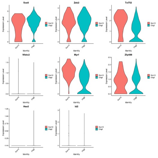
(2) In Figure 1B it appears that the Sox10- MBP+ tdTomato+ cells decreases from D12 to D14. Does this make sense considering MBP is a marker of more mature OLCs?
Thank you for this comment. To address this, we compared the number of MBP+tdTomato+ Sox10 cells across reprogramming timepoints. We saw no difference between the number of MBP+tdTomato+ OLs at D12 and D14 (Author response image 2, p = 0.2314). However, we do see a [nonsignificant] decrease in MBP+tdTomato+ Sox10 cells from D12 to D22 (Manuscript Supplementary Figure 3B, Author response image 2, p= 0.0543), which suggests that culture conditions are not optimal for longer-term cell survival [2], [3], [4].
Author response image 2.
Comparison of Sox10- induced MBP+tdTomato+ iOLCs over time. Quantification of MBP<sup>+</sup>tdTomato<sup>+</sup> iOLs in Sox10 cultures at D8 (n=5), D10 (n=5), D12 (n=5), D14 (n=7) and D22 (n=3) post transduction. Data are presented as mean ± SEM, each data point represents one individual cell culture experiment, Brown-Forsythe and Welch ANOVA on transformed percentages with Dunnett’s T3 multiple comparisons test (*= p<0.05).
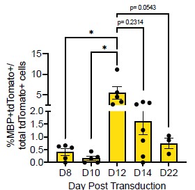
(3) Previous studies have shown that MBP expression and myelination in vitro occurs at the earliest around 4-6 weeks of culturing. When assessing whether further maturation would increase MBP positivity, authors only cultured cells up to 22 DPT and saw no significant increase. Has a lengthier culture timeline been attempted?
We agree with the Reviewer that previous studies of pluripotent stem cell derived (hESCs or iPSCs) have shown MBP+ OLCs in vitro around 4-6 weeks [5], [6], [7]. However, studies of neural stem cells [8] or fibroblasts [9] conversion show OLC appearance after 7 and 24 days, respectively, demonstrating that OLCs can be generated in vitro within 1-3 weeks of plating. Moreover, as noted above in response to #2, we see fewer MBP+ cells at 22DPT, suggesting that extended time in culture may require additional factors for support. Therefore, we did not attempt longer timepoints.
(4) Figure S4D is described as "examples of tdTomatonegzsGreen+OLCmarker+ cells that arose from a tdTomatoneg cell with an astrocyte morphology." The zsGreen+ tdTomato- cell is not convincingly of "astrocyte morphology"; it could be a bipolar OLC. To strengthen the conclusions and remove this subjectivity, more extensive characterizations of astrocyte versus OLC morphology in the introduction or results are warranted. This would make this observation more convincing since there is clearly an overlap in the characteristics of these cell types.
We thank the reviewer for this excellent suggestion. To assess astrocyte morphology, we measured the cell size, nucleus size, number of branches and branch thickness of 70 Aldh1l1+tdTomato+ astrocytes in tamoxifen-labelled Aldh1l1-CreERT2;Ai14 cultures (new Supplemental Table 1). To assess OPC morphology, we performed IHC for PDGFRa in iOLC cultures and measured the same parameters in 70 PDGFRa+ OPCs (new Supplemental Table 1). We found that astrocytes were characterized by larger branch thickness, cell length and nucleus size, while OPCs showed a larger number of branches (new Supplemental Figure 1, and Author response image 3 below). Based on this framework, the AAV9-GFAP::zsGreen<sup>pos</sup>Aldh1l1-tdTomato<sup>neg</sup> and AAV9-GFAP::zsGreen<sup>pos</sup>Aldh1l1-tdTomato<sup>pos</sup>starting cells tracked fall within the bounds of ‘astrocytes’. We have revised the manuscript to include this more rigorous characterization (Line 119-124, Page 4; Line 307-312, Page 9; Line 323-326, Page 9). We also demonstrate (below) that the GFAP::zsGreen<sup>pos</sup> Aldh1l1-tdTomato<sup>pos</sup> and GFAP::zsGreen<sup>pos</sup>Aldh1l1-tdTomato<sup>neg</sup> starting cell depicted in Figure 2G and Supplemental Figure 5D is consistent with astrocyte morphology (Author response image 3).
Author response image 3.
Morphological characterization of astrocytes, oligodendrocyte lineage cells, and starting cells. Quantification of the (A) cell length, (B) nucleus size, (C) number of branches, and (D) branch thickness iAldh1l1+tdTomato+ and PDGFRα+ OPCs (n= 70 per cell type, data are presented as mean ± SEM). Orange line indicates parameter value for GFAP::zsGreen<sup>pos</sup>Aldh1l1-tdTomato<sup>pos</sup> starting cell in Figure 2G. Green line indicates parameter value for GFAP::zsGreen<sup>pos</sup> Aldh1l1-tdTomato<sup>neg</sup> starting cell in Supplemental Figure 5D.
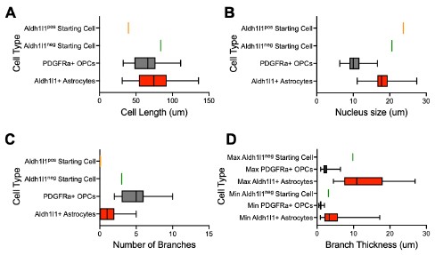
Reviewer #2 (Public Review):
The study by Bajohr investigates the important question of whether astrocytes can generate oligodendrocytes by direct lineage conversion (DLR). The authors ectopically express three transcription factors - Sox10, Olig2 and Nkx6.2 - in cultured postnatal mouse astrocytes and use a combination of Aldh1|1-astrocyte fate mapping and live cell imaging to demonstrate that Sox10 converts astrocytes to MBP+ oligodendrocytes, whereas Olig2 expression converts astrocytes to PDFRalpha+ oligodendrocyte progenitor cells. Nkx6.2 does not induce lineage conversion. The authors use single-cell RNAseq over 14 days post-transduction to uncover molecular signatures of newly generated iOLs.
The potential to convert astrocytes to oligodendrocytes has been previously analyzed and demonstrated. Despite the extensive molecular characterization of the direct astrocyteoligodendrocyte lineage conversion, the paper by Bajohr et al. does not represent significant progress. The entire study is performed in cultured cells, and it is not demonstrated whether this lineage conversion can be induced in astrocytes in vivo, particularly at which developmental stage (postnatal, adult?) and in which brain region. The authors also state that generating oligodendrocytes from astrocytes could be relevant for oligodendrocyte regeneration and myelin repair, but they don't demonstrate that lineage conversion can be induced under pathological conditions, particularly after white matter demyelination. Specific issues are outlined below.
We thank the reviewer for this summary. We agree that there are a handful of reports of astrocytelike cells to OLC conversion [10], [11]. However, our study is the first study to confirm bonafide astrocyte to OLC conversion, which is important given the recent controversy in the field of in vivo astrocyte to neuron reprogramming [12]. In addition, the extensive characterization of the molecular timeline of reprogramming, highlights that although conversion of astrocytes is possible by ectopic expression of any of the three factors, the subtypes of astrocytes converted and maturity of OLCs produced may vary depending on the choice of TF delivered. Our findings will inform future in vivo studies of iOLC generation that aim to understand the impact of brain region, age, pathology, and sex, which are especially important given the diversity of astrocyte responses to disease [13], [14], [15].
(1) The authors perform an extensive characterization of Sox10-mediated DLR by scRNAseq and demonstrate a clear trajectory of lineage conversion from astrocytes to terminally differentiated MBP+ iOLCs. A similar type of analysis should be performed after Olig2 transduction, to determine whether transcriptomics of olig2 conversion overlaps with any phase of sox10 conversion.
We thank the Reviewer for this excellent comment. We chose to include an in-depth analysis of Sox10 in the manuscript, as Sox10-transduced cultures showed a higher percentage of mature iOLCs compared to Olig2 in our studies. We have added this specific rationale to the manuscript (Line 329-330-Page 9).
Nonetheless, we also agree that understanding the underpinnings of Olig2-mediated conversion is important. Therefore, we used Cell Oracle [16] to understand the regulation of cell identity by Olig2. in silico overexpression of Olig2 in our control time course dataset (D0, D3, D8 and D14) showed cell movement from cluster 1, characterized by astrocyte genes [Mmd2[17], Entpd2[18], H2-D1[19]], towards cluster 5, characterized by OPC genes [Pdgfra[20], Myt1[21]] validating astrocyte to OLC conversion by Olig2 (Author response image 4).
We hypothesize that reprogramming via Sox10 and Olig2 take different conversion paths to oligodendrocytes for the following reasons.
(1) Differential astrocyte gene expression at D14 when cells are exposed to Sox10 and Olig2 (Manuscript Figure 1D-E [Sox10 characterized by Lcn2[19], C3[19]; Olig2 characterized by Slc6a11[22], Slc1a2[23]].
(2) Differential expression of key OLC gene regulatory network genes at D14 between cells treated with Sox10 and Olig2 (Author response image 1).
Author response image 4.
in silico modeling of Olig2 reprogramming (A) UMAP clustering of Cre control treated cells from 0, 3, 8, and 14 days post transduction (DPT). (B) UMAP clustering from (A) overlayed with timepoint and treatment group. (C) Cell Oracle modeling of predicted cell trajectories following Olig2 knock in (KI), overlaid onto UMAP plot. Arrows indicate cell movement prediction with Olig2 KI perturbation.
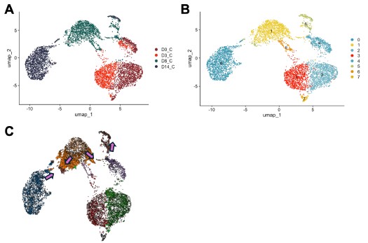
(2) A complete immunohistochemical characterization of the cultures should be performed at different time points after Sox10 and Olig2 transduction to confirm OL lineage cell phenotypes.
We performed a complete immunohistochemical characterization of Ai14 cultures transduced with GFAP::Sox10-Cre and GFAP::Olig2-Cre. This system allows permanent labelling and therefore, enabled the tracking of transduced cells through the process or DLR, which we believe is the most appropriate way to characterize iOLC conversion efficiencies. We then confirmed the conversion of Aldh1l1+ astrocytes in Aldh1l1-CreERT2;Ai14 cultures transduced with GFAP::Sox10-zsGreen and GFAP::Olig2-zsGreen. In this system, GFAP drives the expression of zsGreen, and therefore, may not faithfully track all cells and lead to an underestimate of the numbers of converted cells. For example, iOLCs from Aldh1l1<sup>neg</sup> astrocytes or iOLCs that have lost zsGreen expression following conversion. Therefore we use this system only to confirm astrocyte origin.
Nonetheless, we appreciate this comment and recognize that there may be differences in conversion efficiencies when analyzing Aldh1l1+ astrocytes versus all transduced cells. Therefore, we have softened the language in the manuscript (see below) regarding Olig2 and Sox10 generating different OLC phenotypes and now claim iOLC generation from both Sox10 and Olig2. We thank the Reviewer for this comment, and believe it has strengthened the discussion.
Line 240, Page 7
Line 261-263, Page 8
Line 304-307, Page 8/9
Line 413-414, Page 11
References
(1) E. Sock and M. Wegner, “Using the lineage determinants Olig2 and Sox10 to explore transcriptional regulation of oligodendrocyte development,” Dev Neurobiol, vol. 81, no. 7, pp. 892–901, Oct. 2021, doi: 10.1002/dneu.22849.
(2) B. A. Barres, M. D. Jacobson, R. Schmid, M. Sendtner, and M. C. Raff, “Does oligodendrocyte survival depend on axons?,” Current Biology, vol. 3, no. 8, pp. 489–497, Aug. 1993, doi: 10.1016/0960-9822(93)90039-Q.
(3) A.-N. Cho et al., “Aligned Brain Extracellular Matrix Promotes Differentiation and Myelination of Human-Induced Pluripotent Stem Cell-Derived Oligodendrocytes,” ACS Appl. Mater. Interfaces, vol. 11, no. 17, pp. 15344–15353, May 2019, doi: 10.1021/acsami.9b03242.
(4) E. G. Hughes and M. E. Stockton, “Premyelinating Oligodendrocytes: Mechanisms Underlying Cell Survival and Integration,” Front. Cell Dev. Biol., vol. 9, Jul. 2021, doi: 10.3389/fcell.2021.714169.
(5) M. Ehrlich et al., “Rapid and efficient generation of oligodendrocytes from human induced pluripotent stem cells using transcription factors,” Proc Natl Acad Sci U S A, vol. 114, no. 11, pp. E2243–E2252, Mar. 2017, doi: 10.1073/pnas.1614412114.
(6) Y. Liu, P. Jiang, and W. Deng, “OLIG gene targeting in human pluripotent stem cells for motor neuron and oligodendrocyte differentiation,” Nat Protoc, vol. 6, no. 5, pp. 640–655, May 2011, doi: 10.1038/nprot.2011.310.
(7) S. A. Goldman and N. J. Kuypers, “How to make an oligodendrocyte,” Development, vol. 142, no. 23, pp. 3983–3995, Dec. 2015, doi: 10.1242/dev.126409.
(8) M. Faiz, N. Sachewsky, S. Gascón, K. W. A. Bang, C. M. Morshead, and A. Nagy, “Adult Neural Stem Cells from the Subventricular Zone Give Rise to Reactive Astrocytes in the Cortex after Stroke,” Cell Stem Cell, vol. 17, no. 5, pp. 624–634, Nov. 2015, doi:10.1016/j.stem.2015.08.002.
(9) F. J. Najm et al., “Transcription factor–mediated reprogramming of fibroblasts to expandable, myelinogenic oligodendrocyte progenitor cells,” Nat Biotechnol, vol. 31, no. 5, pp. 426–433, May 2013, doi: 10.1038/nbt.2561.
(10) A. Mokhtarzadeh Khanghahi, L. Satarian, W. Deng, H. Baharvand, and M. Javan, “In vivo conversion of astrocytes into oligodendrocyte lineage cells with transcription factor Sox10; Promise for myelin repair in multiple sclerosis,” PLoS One, vol. 13, no. 9, p. e0203785, Sep. 2018, doi: 10.1371/journal.pone.0203785.
(11) S. Farhangi, S. Dehghan, M. Totonchi, and M. Javan, “In vivo conversion of astrocytes to oligodendrocyte lineage cells in adult mice demyelinated brains by Sox2,” Mult Scler Relat Disord, vol. 28, pp. 263–272, Feb. 2019, doi: 10.1016/j.msard.2018.12.041.
(12) L.-L. Wang, C. Serrano, X. Zhong, S. Ma, Y. Zou, and C.-L. Zhang, “Revisiting astrocyte to neuron conversion with lineage tracing in vivo,” Cell, vol. 184, no. 21, pp. 5465-5481.e16, Oct. 2021, doi: 10.1016/j.cell.2021.09.005.
(13) I Matias, J. Morgado, and F. C. A. Gomes, “Astrocyte Heterogeneity: Impact to Brain Aging and Disease,” Front. Aging Neurosci., vol. 11, Mar. 2019, doi: 10.3389/fnagi.2019.00059.
(14) N. Habib et al., “Disease-associated astrocytes in Alzheimer’s disease and aging,” Nat Neurosci, vol. 23, no. 6, pp. 701–706, Jun. 2020, doi: 10.1038/s41593-020-0624-8.
(15) M. A. Wheeler et al., “MAFG-driven astrocytes promote CNS inflammation,” Nature, vol. 578, no. 7796, pp. 593–599, Feb. 2020, doi: 10.1038/s41586-020-1999-0.
(16) K. Kamimoto, B. Stringa, C. M. Hoffmann, K. Jindal, L. Solnica-Krezel, and S. A. Morris, “Dissecting cell identity via network inference and in silico gene perturbation,” Nature, vol. 614, no. 7949, pp. 742–751, Feb. 2023, doi: 10.1038/s41586-022-05688-9.
(17) P. Kang et al., “Sox9 and NFIA coordinate a transcriptional regulatory cascade during the initiation of gliogenesis,” Neuron, vol. 74, no. 1, pp. 79–94, Apr. 2012, doi:10.1016/j.neuron.2012.01.024.
(18) K. Saito et al., “Microglia sense astrocyte dysfunction and prevent disease progression in an Alexander disease model,” Brain, vol. 147, no. 2, pp. 698–716, Nov. 2023, doi:10.1093/brain/awad358.
(19) S. A. Liddelow et al., “Neurotoxic reactive astrocytes are induced by activated microglia,” Nature, vol. 541, no. 7638, pp. 481–487, Jan. 2017, doi: 10.1038/nature21029.
(20) Q. Zhu et al., “Genetic evidence that Nkx2.2 and Pdgfra are major determinants of the timing of oligodendrocyte differentiation in the developing CNS,” Development, vol. 141, no. 3, pp. 548–555, Feb. 2014, doi: 10.1242/dev.095323.
(21) J. A. Nielsen, J. A. Berndt, L. D. Hudson, and R. C. Armstrong, “Myelin transcription factor 1 (Myt1) modulates the proliferation and differentiation of oligodendrocyte lineage cells,” Mol Cell Neurosci, vol. 25, no. 1, pp. 111–123, Jan. 2004, doi:10.1016/j.mcn.2003.10.001.
(22) J. Liu, X. Feng, Y. Wang, X. Xia, and J. C. Zheng, “Astrocytes: GABAceptive and GABAergic Cells in the Brain,” Front. Cell. Neurosci., vol. 16, Jun. 2022, doi:10.3389/fncel.2022.892497.
(23) A. Sharma et al., “Divergent roles of astrocytic versus neuronal EAAT2 deficiency on cognition and overlap with aging and Alzheimer’s molecular signatures,” Proceedings of the National Academy of Sciences, vol. 116, no. 43, pp. 21800–21811, Oct. 2019, doi:10.1073/pnas.1903566116
Ser libre para el republicanismo tiene que ver con la capacidad para ser dueños y amos de nuestras propias vidas en sentido pleno. Esta idea de libertad dentro del marco del pensamiento republicano está ligada a otros conceptos que son fundamentales, como el de la virtud cívica. Ser virtuosos dentro de una república implica el deber de involucrarse en los asuntos públicos y, por tanto, en el gobierno de la comunidad política (en distinto grado).
RRID:CVCL_0620
DOI: 10.1038/s44320-025-00160-y
Resource: (BCRC Cat# 60549, RRID:CVCL_0620)
Curator: @evieth
SciCrunch record: RRID:CVCL_0620
RRID:AB_10709300
DOI: 10.1038/s44320-025-00160-y
Resource: (Santa Cruz Biotechnology Cat# sc-271682, RRID:AB_10709300)
Curator: @scibot
SciCrunch record: RRID:AB_10709300
RRID:AB_2078685
DOI: 10.1038/s44320-025-00160-y
Resource: (Cell Signaling Technology Cat# 2561, RRID:AB_2078685)
Curator: @scibot
SciCrunch record: RRID:AB_2078685
RRID:AB_2736361
DOI: 10.1038/s44320-025-00160-y
Resource: None
Curator: @scibot
SciCrunch record: RRID:AB_2736361
RRID:CVCL_0031
DOI: 10.1038/s44320-025-00160-y
Resource: (NCI-DTP Cat# MCF7, RRID:CVCL_0031)
Curator: @scibot
SciCrunch record: RRID:CVCL_0031
RRID:AB_2078855
DOI: 10.1038/s44320-025-00160-y
Resource: (Cell Signaling Technology Cat# 2506, RRID:AB_2078855)
Curator: @scibot
SciCrunch record: RRID:AB_2078855
RRID:SCR_024202
DOI: 10.1038/s44320-025-00160-y
Resource: python-bx (RRID:SCR_024202)
Curator: @scibot
SciCrunch record: RRID:SCR_024202
RRID:AB_627238
DOI: 10.1038/s44320-025-00160-y
Resource: (Santa Cruz Biotechnology Cat# sc-6248, RRID:AB_627238)
Curator: @scibot
SciCrunch record: RRID:AB_627238
RRID:SCR_014782
DOI: 10.1038/s44320-025-00160-y
Resource: OncoKB (RRID:SCR_014782)
Curator: @scibot
SciCrunch record: RRID:SCR_014782
RRID:CVCL_0062361
DOI: 10.1038/s44320-025-00160-y
Resource: None
Curator: @evieth
SciCrunch record: RRID:CVCL_0062
RRID:IMSR_JAX:004847
DOI: 10.1038/s41593-025-02094-y
Resource: (IMSR Cat# JAX_004847,RRID:IMSR_JAX:004847)
Curator: @scibot
SciCrunch record: RRID:IMSR_JAX:004847
RRID:IMSR_JAX
DOI: 10.1038/s41593-025-02094-y
Resource: None
Curator: @evieth
SciCrunch record: RRID:IMSR_JAX:029655
Es también una estrategiaretórica y un método político para el que yo pido más respeto dentro del feminismosocialista.
La ironía es un recurso estilístico importante porque no presenta la información como una verdad absoluta, sino que muestra como un discurso puede ser contradictorio y ambiguo en aquello que desconoce. Además, sirve de unión entre comunidades marginales y desafía las normas establecidas.
No existenada en el hecho de ser ‘mujer’ que una de manera natural a las mujeres. No existeincluso el estado de ’ser’ mujer, que, en sí mismo, es una categoría enormementecompleja construida dentro de contestados discursos científicosexuales y de otrasprácticas sociales
La autora revela que el propio concepto de "mujer" es problemático, ya que la experiencia femenina se construye en base a diferentes factores como son la raza, la clase social o la sexualidad. Por tanto, un feminismo inclusivo debería recoger todas las realidades sociales, basándose en políticas de afinidad y coaliciones donde no sea necesario identificarse con un problema, pero sí ser consciente de ello y aliarse para luchar contra él.
Author response:
The following is the authors’ response to the current reviews.
Reviewer #2 (Public review):
Summary:
Using a gerbil model, the authors tested the hypothesis that loss of synapses between sensory hair cells and auditory nerve fibers (which may occur due to noise exposure or aging) affects behavioral discrimination of the rapid temporal fluctuations of sounds. In contrast to previous suggestions in the literature, their results do not support this hypothesis; young animals treated with a compound that reduces the number of synapses did not show impaired discrimination compared to controls. Additionally, their results from older animals showing impaired discrimination suggest that age-related changes aside from synaptopathy are responsible for the age-related decline in discrimination.
Strengths:
(1) The rationale and hypothesis are well-motivated and clearly presented.
(2) The study was well conducted with strong methodology for the most part, and good experimental control. The combination of physiological and behavioral techniques is powerful and informative. Reducing synapse counts fairly directly using ouabain is a cleaner design than using noise exposure or age (as in other studies), since these latter modifiers have additional effects on auditory function.
(3) The study may have a considerable impact on the field. The findings could have important implications for our understanding of cochlear synaptopathy, one of the most highly researched and potentially impactful developments in hearing science in the past fifteen years.
Weaknesses:
(1) I have concerns that the gerbils may not have been performing the behavioral task using temporal fine structure information.
Human studies using the same task employed a filter center frequency that was (at least) 11 times the fundamental frequency (Marmel et al., 2015; Moore and Sek, 2009). Moore and Sek wrote: "the default (recommended) value of the centre frequency is 11F0." Here, the center frequency was only 4 or 8 times the fundamental frequency (4F0 or 8F0). Hence, relative to harmonic frequency, the harmonic spacing was considerably greater in the present study. However, gerbil auditory filters are thought to be broader than those in human. In the revised version of the manuscript, the authors provide modelling results suggesting that the excitation patterns were discriminable for the 4F0 conditions, but may not have been for the 8F0 conditions. These results provide some reassurance that the 8F0 discriminations were dependent on temporal cues, but the description of the model lacks detail. Also, the authors state that "thus, for these two conditions with harmonic number N of 8 the gerbils cannot rely on differences in the excitation patterns but must solve the task by comparing the temporal fine structure." This is too strong. Pulsed tone intensity difference limens (the reference used for establishing whether or not the excitation pattern cues were usable) may not be directly comparable to profile-analysis-like conditions, and it has been argued that frequency discrimination may be more sensitive to excitation pattern cues than predicted from a simple comparison to intensity difference limens (Micheyl et al. 2013, https://doi.org/10.1371/journal.pcbi.1003336
We can assume that our conclusions based on the excitation patterns are adequate when putting gerbil auditory filter data, frequency difference limens and intensity difference limens together into perspective. Kittel et al. (2002) observed an about factor 2 larger auditory-filter bandwidth in the gerbil than in humans reducing the number of independent frequency channels in the analysis of excitation patterns. The gerbil frequency-difference limen for pure tones being an indicator for the sensitivity to make use of excitation patterns is more than an order of magnitude larger than the corresponding human frequency difference limen (Klinge and Klump 2009, https://doi.org/10.1121/1.3021315). Finally, the gerbil intensity-difference limen of 2.8 dB observed for 1-kHz pure tones is considerably larger than the 0.75 dB observed for humans in the same study (Sinnott et al. 1992). Thus, taken together these lines of evidence indicate that our conclusions regarding the potential use of excitation patterns are not too strong.
I'm also somewhat concerned that the masking noise used in the present study was too low in level to mask cochlear distortion products. Based on their excitation pattern modelling, the authors state (without citation) that "since the level of excitation produced by the pink noise is less than 30 dB below that produced by the complex tones, distortion products will be masked." The basis for this claim is not clear. In human, distortion products may be only ~20 dB below the levels of the primaries (referenced to an external sound masker / canceller, which is appropriate, assuming that the modelling reported in the present paper did not include middle-ear effects; see Norman-Haignere and McDermott, 2016, doi: 10.1016/j.neuroimage.2016.01.050). Oxenham et al. (2009, doi: 10.1121/1.3089220) provide further cautionary evidence on the potential use of distortion product cues when the background noise level is too low (in their case the relative level of the noise in the compromised condition was only a little below that used in the present study). The masking level used in the present study may have been sufficient, but it would be useful to have some further reassurance on this point.
In the method section, we provide the citation for estimating the size of the distortion products and the estimated signal-to-noise ratio making the basis for our estimates clear.
We consulted Oxenham et al. (2009, doi: 10.1121/1.3089220) who suggested that distortion products may have been used in human subjects. However, in Fig. 1 of their paper, they convincingly demonstrate that even for humans that have more narrow auditory filters than gerbils, spectral cues cannot be used to evaluate the frequency shift in harmonic complex tones. We are confident that the same limitation applies to gerbils that have wider auditory filters than humans and a lower ability to use spectral cues as indicated by their higher frequency-difference limens and intensity-difference limens compared to humans.
(2) The synapse reductions in the high ouabain and old groups were relatively small (mean of 19 synapses per hair cell compared to 23 in the young untreated group). In contrast, in some mouse models of the effects of noise exposure or age, a 50% reduction in synapses is observed, and in the human temporal bone study of Wu et al. (2021, https://doi.org/10.1523/JNEUROSCI.3238-20.2021) the age-related reduction in auditory nerve fibres was ~50% or greater for the highest age group across cochlear location. It could be simply that the synapse loss in the present study was too small to produce significant behavioral effects. Hence, although the authors provide evidence that in the gerbil model the age-related behavioral effects are not due to synaptopathy, this may not translate to other species (including human).
(3) The study was not pre-registered, and there was no a priori power calculation, so there is less confidence in replicability than could have been the case. Only three old animals were used in the behavioral study, which raises concerns about the reliability of comparisons involving this group.
Reviewer #3 (Public review):
This study is a part of the ongoing series of rigorous work from this group exploring neural coding deficits in the auditory nerve, and dissociating the effects of cochlear synaptopathy from other age-related deficits. They have previously shown no evidence of phase-locking deficits in the remaining auditory nerve fibers in quiet-aged gerbils. Here, they study the effects of aging on the perception and neural coding of temporal fine structure cues in the same Mongolian gerbil model.
They measure TFS coding in the auditory nerve using the TFS1 task which uses a combination of harmonic and tone-shifted inharmonic tones which differ primarily in their TFS cues (and not the envelope). They then follow this up with a behavioral paradigm using the TFS1 task in these gerbils. They test young normal hearing gerbils, aged gerbils, and young gerbils with cochlear synaptopathy induced using the neurotoxin ouabain to mimic synapse losses seen with age.
In the behavioral paradigm, they find that aging is associated with decreased performance compared to the young gerbils, whereas young gerbils with similar levels of synapse loss do not show these deficits. When looking at the auditory nerve responses, they find no differences in neural coding of TFS cues across any of the groups. However, aged gerbils show an increase in the representation of periodicity envelope cues (around f0) compared to young gerbils or those with induced synapse loss. The authors hence conclude that synapse loss by itself doesn't seem to be important for distinguishing TFS cues, and rather the behavioral deficits with age are likely having to do with the misrepresented envelope cues instead.
The manuscript is well written, and the data presented are robust. Some of the points below will need to be considered while interpreting the results of the study, in its current form. These considerations are addressable if deemed necessary, with some additional analysis in future versions of the manuscript.
Spontaneous rates - Figure S2 shows no differences in median spontaneous rates across groups. But taking the median glosses over some of the nuances there. Ouabain (in the Bourien study) famously affects low spont rates first, and at a higher degree than median or high spont rates. It seems to be the case (qualitatively) in figure S2 as well, with almost no units in the low spont region in the ouabain group, compared to the other groups. Looking at distributions within each spont rate category and comparing differences across the groups might reveal some of the underlying causes for these changes. Given that overall, the study reports that low-SR fibers had a higher ENV/TFS log-z-ratio, the distribution of these fibers across groups may reveal specific effects of TFS coding by group.
[Update: The revised manuscript has addressed these issues]
Threshold shifts - It is unclear from the current version if the older gerbils have changes in hearing thresholds, and whether those changes may be affecting behavioral thresholds. The behavioral stimuli appear to have been presented at a fixed sound level for both young and aged gerbils, similar to the single unit recordings. Hence, age-related differences in behavior may have been due to changes in relative sensation level. Approaches such as using hearing thresholds as covariates in the analysis will help explore if older gerbils still show behavioral deficits.
[Update: The issue of threshold shifts with aging gerbils is still unresolved in my opinion. From the revised manuscript, it appears that aged gerbils have a 36dB shift in thresholds. While the revised manuscript provides convincing evidence that these threshold shifts do not affect the auditory nerve tuning properties, the behavioral paradigm was still presented at the same sound level for young and aged animals. But a potential 36 dB change in sensation level may affect behavioral results. The authors may consider adding thresholds as covariates in analyses or present any evidence that behavioral thresholds are plateaued along that 30dB range].
Since we do not have behavioural detection thresholds from our individual animals, only CAP thresholds that represent the auditory-nerve data and cannot be translated to behavioural thresholds directly, we want to refrain from using these indirect measures as covariates in the present analysis. In addition, the study by Hamann et al. (2002, https://doi.org/10.1016/S0378-5955(02)00454-9) indicates that age-related behavioural threshold increases are smaller than threshold increases obtained from auditory brainstem response measurements. Finally, statistical analyses on very small samples can be unreliable due to problems of power, generalisability, and susceptibility to outliers.
Moore and Sek (2009) in their paper on the TFS1 test pointed out that the effect of signal level on the TFS1 threshold in normal hearing human subjects was small when the signal-to-noise ratio between the broadband masking noise and the complex tone was kept constant. Furthermore, the masking noise will raise the thresholds of normal hearing gerbils and old gerbils with an audibility threshold increase to about the same signal-to-noise ratio. Thus, as long as the signal remains audible to the behaviourally tested gerbil which can be expected at an overall signal level of 68 dB SPL, we expect little effect of raised audibility thresholds on the TFS1 threshold. The lack of temporal processing deficits in the auditory-nerve fibers of old, mildly hearing impaired gerbils compared to those in normal hearing young adult gerbils further strengthens this argument.
Task learning in aged gerbils - It is unclear if the aged gerbils really learn the task well in two of the three TFS1 test conditions. The d' of 1 which is usually used as the criterion for learning was not reached in even the easiest condition for aged gerbils in all but one condition for the aged gerbils (Fig. 5H) and in that condition, there doesn't seem to be any age-related deficits in behavioral performance (Fig. 6B). Hence dissociating the inability to learn the task from the inability to perceive TFS 1 cues in those animals becomes challenging.
[Update: The revised manuscript sufficiently addresses these issues, with the caveat of hearing threshold changes affecting behavioral thresholds mentioned above].
As we argued above, an audibility threshold increase in the old gerbils is unlikely to explain the raised TFS1 thresholds in the old gerbils.
Increased representation of periodicity envelope in the AN - the mechanisms for increased representation of periodicity envelope cues is unclear. The authors point to some potential central mechanisms but given that these are recordings from the auditory nerve what central mechanisms these may be is unclear. If the authors are suggesting some form of efferent modulation only at the f0 frequency, no evidence for this is presented. It appears more likely that the enhancement may be due to outer hair cell dysfunction (widened tuning, distorted tonotopy). Given this increased envelope coding, the potential change in sensation level for the behavior (from the comment above), and no change in neural coding of TFS cues across any of the groups, a simpler interpretation may be -TFS coding is not affected in remaining auditory nerve fibers after age-related or ouabain induced synapse loss, but behavioral performance is affected by altered outer hair cell dysfunction with age.
[Update: The revised manuscript has addressed these issues]
Emerging evidence seems to suggest that cochlear synaptopathy and/or TFS encoding abilities might be reflected in listening effort rather than behavioral performance. Measuring some proxy of listening effort in these gerbils (like reaction time) to see if that has changed with synapse loss, especially in the young animals with induced synaptopathy, would make an interesting addition to explore perceptual deficits of TFS coding with synapse loss.
[Update: The revised manuscript has addressed these issues]
Reviewer #3 (Recommendations for the authors):
Thank you for your revisions. They largely address most of my initial concerns. The issue of threshold shifts potentially affecting behavioral thresholds still remains unresolved in my opinion. The new data about unaltered tuning curves is convincing that the auditory nerve fiber recordings are unaffected by threshold shifts. But am I correct in my understanding that the threshold shift with age was 36 dB relative to the young (L168)? If so, wouldn't the fact that behavior was performed at 68 dB SPL regardless of group affect the behavioral thresholds with age? Is there any additional evidence that suggests that behavioral performance plateaus along that ~30dB range that the authors could include to strengthen this claim?
In our response above to reviewer #3 and to reviewer #2 we provided additional arguments why we think that an audibility threshold increase in old gerbils cannot explain their compromised TFS1 thresholds.
The following is the authors’ response to the original reviews.
Reviewer #1(Public review)
Summary:
The authors investigate the effects of aging on auditory system performance in understanding temporal fine structure (TFS), using both behavioral assessments and physiological recordings from the auditory periphery, specifically at the level of the auditory nerve. This dual approach aims to enhance understanding of the mechanisms underlying observed behavioral outcomes. The results indicate that aged animals exhibit deficits in behavioral tasks for distinguishing between harmonic and inharmonic sounds, which is a standard test for TFS coding. However, neural responses at the auditory nerve level do not show significant differences when compared to those in young, normalhearing animals. The authors suggest that these behavioral deficits in aged animals are likely attributable to dysfunctions in the central auditory system, potentially as a consequence of aging. To further investigate this hypothesis, the study includes an animal group with selective synaptic loss between inner hair cells and auditory nerve fibers, a condition known as cochlear synaptopathy (CS).CS is a pathology associated with aging and is thought to be an early indicator of hearing impairment. Interestingly, animals with selective CS showed physiological and behavioral TFS coding similar to that of the young normal-hearing group, contrasting with the aged group's deficits. Despite histological evidence of significant synaptic loss in the CS group, the study concludes that CS does not appear to affect TFS coding, either behaviorally or physiologically.
We agree with the reviewer’s summary.
Strengths:
This study addresses a critical health concern, enhancing our understanding of mechanisms underlying age-related difficulties in speech intelligibility, even when audiometric thresholds are within normal limits. A major strength of this work is the comprehensive approach, integrating behavioral assessments, auditory nerve (AN) physiology, and histology within the same animal subjects. This approach enhances understanding of the mechanisms underlying the behavioral outcomes and provides confidence in the actual occurrence of synapse loss and its effects. The study carefully manages controlled conditions by including five distinct groups: young normal-hearing animals, aged animals, animals with CS induced through low and high doses, and a sham surgery group. This careful setup strengthens the study's reliability and allows for meaningful comparisons across conditions. Overall, the manuscript is well-structured, with clear and accessible writing that facilitates comprehension of complex concepts.
Weaknesses:
The stimulus and task employed in this study are very helpful for behavioral research, and using the same stimulus setup for physiology is advantageous for mechanistic comparisons. However, I have some concerns about the limitations in auditory nerve (AN) physiology. Due to practical constraints, it is not feasible to record from a large enough population of fibers that covers a full range of best frequencies (BFs) and spontaneous rates (SRs) within each animal. This raises questions about how representative the physiological data are for understanding the mechanism in behavioral data. I am curious about the authors' interpretation of how this stimulus setup might influence results compared to methods used by Kale and Heinz (2010), who adjusted harmonic frequencies based on the characteristic frequency (CF) of recorded units. While, the harmonic frequencies in this study are fixed across all CFs, meaning that many AN fibers may not be tuned closely to the stimulus frequencies. If units are not responsive to the stimulus further clarification on detecting mistuning and phase locking to TFS effects within this setup would be valuable. Since the harmonic frequencies in this study are fixed across all CFs, this means that many AN fibers may not be tuned closely to the stimulus frequencies, adding sampling variability to the results.
We chose the stimuli for the AN recordings to be identical to the stimuli used in the behavioral evaluation of the perceptual sensitivity. Only with this approach can we directly compare the response of the population of AN fibers with perception measured in behavior.
The stimuli are complex, i.e., comprise of many frequency components AND were presented at 68 dB SPL. Thus, the stimuli excite a given fiber within a large portion of the fiber’s receptive field. Furthermore, during recordings, we assured ourselves that fibers responded to the stimuli by audiovisual control. Otherwise it would have cost valuable recording time to record from a nonresponsive AN fiber.
Given the limited number of units per condition-sometimes as few as three for certain conditions - I wonder if CF-dependent variability might impact the results of the AN data in this study and discussing this factor can help with better understanding the results. While the use of the same stimuli for both behavioral and physiological recordings is understandable, a discussion on how this choice affects interpretation would be beneficial. In addition a 60 dB stimulus could saturate high spontaneous rate (HSR) AN fibers, influencing neural coding and phase-locking to TFS. Potentially separating SR groups, could help address these issues and improve interpretive clarity.
A deeper discussion on the role of fiber spontaneous rate could also enhance the study. How might considering SR groups affect AN results related to TFS coding? While some statistical measures are included in the supplement, a more detailed discussion in the main text could help in interpretation. We do not think that it will be necessary to conduct any statistical analysis in addition to that already reported in the supplement.
We considered moving some supplementary information back into the main manuscript but decided against it. Our single-unit sample was not sufficient, i.e. not all subpopulations of auditory-nerve fibers were sufficiently sampled for all animal treatment groups, to conclusively resolve every aspect that may be interesting to explore. The power of our approach lies in the direct linkage of several levels of investigation – cochlear synaptic morphology, single-unit representation and behavioral performance – and, in the main manuscript, we focus on the core question of synaptopathy and its relation to temporal fine structure perception. This is now spelled out clearly in lines 197 - 203 of the main manuscript.
Although Figure S2 indicates no change in median SR, the high-dose treatment group lacks LSR fibers, suggesting a different distribution based on SR for different animal groups, as seen in similar studies on other species. A histogram of these results would be informative, as LSR fiber loss with CS-whether induced by ouabain in gerbils or noise in other animals-is well documented (e.g., Furman et al., 2013).
Figure S2 was revised to avoid overlap of data points and show the distributions more clearly. Furthermore, the sample sizes for LSR and HSR fibers are now provided separately.
Although ouabain effects on gerbils have been explored in previous studies, since these data already seems to be recorded for the animal in this study, a brief description of changes in auditory brainstem response (ABR) thresholds, wave 1 amplitudes, and tuning curves for animals with cochlear synaptopathy (CS) in this study would be beneficial. This would confirm that ouabain selectively affects synapses without impacting outer hair cells (OHCs). For aged animals, since ABR measurements were taken, comparing hearing differences between normal and aged groups could provide insights into the pathologies besides CS in aged animals. Additionally, examining subject variability in treatment effects on hearing and how this correlates with behavior and physiology would yield valuable insights. If limited space maybe a brief clarification or inclusion in supplementary could be good enough.
We thank the reviewer for this constructive suggestion. The requested data were added in a new section of the Results, entitled “Threshold sensitivity and frequency tuning were not affected by the synapse loss.” (lines 150 – 174). Our young-adult, ouabain-treated gerbils showed no significant elevations of CAP thresholds and their neural tuning was normal. Old gerbils showed the typical threshold losses for individuals of comparable age, and normal neural tuning, confirming previous reports. Thus, there was no evidence for relevant OHC impairments in any of our animal groups.
Another suggestion is to discuss the potential role of MOC efferent system and effect of anesthesia in reducing efferent effects in AN recordings. This is particularly relevant for aged animals, as CS might affect LSR fibers, potentially disrupting the medial olivocochlear (MOC) efferent pathway. Anesthesia could lessen MOC activity in both young and aged animals, potentially masking efferent effects that might be present in behavioral tasks. Young gerbils with functional efferent systems might perform better behaviorally, while aged gerbils with impaired MOC function due to CS might lack this advantage. A brief discussion on this aspect could potentially enhance mechanistic insights.
Thank you for this suggestion. The potential role of olivocochlear efferents is now discussed in lines 597 - 613.
Lastly, although synapse counts did not differ between the low-dose treatment and NH I sham groups, separating these groups rather than combining them with the sham might reveal differences in behavior or AN results, particularly regarding the significance of differences between aged/treatment groups and the young normal-hearing group.
For maximizing statistical power, we combined those groups in the statistical analysis. These two groups did not differ in synapse number, threshold sensitivity or neural tuning bandwidths.
Reviewer #2 (Public review):
Summary:
Using a gerbil model, the authors tested the hypothesis that loss of synapses between sensory hair cells and auditory nerve fibers (which may occur due to noise exposure or aging) affects behavioral discrimination of the rapid temporal fluctuations of sounds. In contrast to previous suggestions in the literature, their results do not support this hypothesis; young animals treated with a compound that reduces the number of synapses did not show impaired discrimination compared to controls. Additionally, their results from older animals showing impaired discrimination suggest that agerelated changes aside from synaptopathy are responsible for the age-related decline in discrimination.
We agree with the reviewer’s summary.
Strengths:
(1) The rationale and hypothesis are well-motivated and clearly presented.
(2) The study was well conducted with strong methodology for the most part, and good experimental control. The combination of physiological and behavioral techniques is powerful and informative. Reducing synapse counts fairly directly using ouabain is a cleaner design than using noise exposure or age (as in other studies), since these latter modifiers have additional effects on auditory function.
(3) The study may have a considerable impact on the field. The findings could have important implications for our understanding of cochlear synaptopathy, one of the most highly researched and potentially impactful developments in hearing science in the past fifteen years.
Weaknesses:
(1) My main concern is that the stimuli may not have been appropriate for assessing neural temporal coding behaviorally. Human studies using the same task employed a filter center frequency that was (at least) 11 times the fundamental frequency (Marmel et al., 2015; Moore and Sek, 2009). Moore and Sek wrote: "the default (recommended) value of the centre frequency is 11F0." Here, the center frequency was only 4 or 8 times the fundamental frequency (4F0 or 8F0). Hence, relative to harmonic frequency, the harmonic spacing was considerably greater in the present study. By my calculations, the masking noise used in the present study was also considerably lower in level relative to the harmonic complex than that used in the human studies. These factors may have allowed the animals to perform the task using cues based on the pattern of activity across the neural array (excitation pattern cues), rather than cues related to temporal neural coding. The authors show that mean neural driven rate did not change with frequency shift, but I don't understand the relevance of this. It is the change in response of individual fibers with characteristic frequencies near the lowest audible harmonic that is important here.
The auditory filter bandwidth of the gerbil is about double that of human subjects. Because of this, the masking noise has a larger overall level than in the human studies in the filter, prohibiting the use of distortion products. The larger auditory filter bandwidth precludes that the gerbils can use excitation patterns, especially in the condition with a center frequency of 1600 Hz and a fundamental of 200 Hz and in the condition with a center frequency of 3200 Hz and a fundamental of 400 Hz. In the condition with a center frequency of 1600 Hz and a fundamental of 400 Hz, it is possible that excitation patterns are exploited. We have now added modeling of the excitation patterns, and a new figure showing their change at the gerbils’ perception threshold, in the discussion of the revised version (lines 440 - 446 and Fig. 8).
The case against excitation pattern cues needs to be better made in the Discussion. It could be that gerbil frequency selectivity is broad enough for this not to be an issue, but more detail needs to be provided to make this argument. The authors should consider what is the lowest audible harmonic in each case for their stimuli, given the level of each harmonic and the level of the pink noise. Even for the 8F0 center frequency, the lowest audible harmonic may be as low as the 4th (possibly even the 3rd). In human, harmonics are thought to be resolvable by the cochlea up to at least the 8th.
This issue is now covered in the discussion, see response to the previous point.
(2) The synapse reductions in the high ouabain and old groups were relatively small (mean of 19 synapses per hair cell compared to 23 in the young untreated group). In contrast, in some mouse models of the effects of noise exposure or age, a 50% reduction in synapses is observed, and in the human temporal bone study of Wu et al. (2021, https://doi.org/10.1523/JNEUROSCI.3238-20.2021) the age-related reduction in auditory nerve fibres was ~50% or greater for the highest age group across cochlear location. It could be simply that the synapse loss in the present study was too small to produce significant behavioral effects. Hence, although the authors provide evidence that in the gerbil model the age-related behavioral effects are not due to synaptopathy, this may not translate to other species (including human). This should be discussed in the manuscript.
We agree that our results apply to moderate synaptopathy, which predominantly characterizes early stages of hearing loss or aged individuals without confounding noise-induced cochlear damage. This is now discussed in lines 486 – 498.
It would be informative to provide synapse counts separately for the animals who were tested behaviorally, to confirm that the pattern of loss across the group was the same as for the larger sample.
Yes, the pattern was the same for the subgroup of behaviorally tested animals. We have added this information to the revised version of the manuscript (lines 137 – 141).
(3) The study was not pre-registered, and there was no a priori power calculation, so there is less confidence in replicability than could have been the case. Only three old animals were used in the behavioral study, which raises concerns about the reliability of comparisons involving this group.
The results for the three old subjects differed significantly from those of young subjects and young ouabain-treated subjects. This indicates a sufficient statistical power, since otherwise no significant differences would be observed.
Reviewer #3 (Public review):
This study is a part of the ongoing series of rigorous work from this group exploring neural coding deficits in the auditory nerve, and dissociating the effects of cochlear synaptopathy from other agerelated deficits. They have previously shown no evidence of phase-locking deficits in the remaining auditory nerve fibers in quiet-aged gerbils. Here, they study the effects of aging on the perception and neural coding of temporal fine structure cues in the same Mongolian gerbil model.
They measure TFS coding in the auditory nerve using the TFS1 task which uses a combination of harmonic and tone-shifted inharmonic tones which differ primarily in their TFS cues (and not the envelope). They then follow this up with a behavioral paradigm using the TFS1 task in these gerbils. They test young normal hearing gerbils, aged gerbils, and young gerbils with cochlear synaptopathy induced using the neurotoxin ouabain to mimic synapse losses seen with age.
In the behavioral paradigm, they find that aging is associated with decreased performance compared to the young gerbils, whereas young gerbils with similar levels of synapse loss do not show these deficits. When looking at the auditory nerve responses, they find no differences in neural coding of TFS cues across any of the groups. However, aged gerbils show an increase in the representation of periodicity envelope cues (around f0) compared to young gerbils or those with induced synapse loss. The authors hence conclude that synapse loss by itself doesn't seem to be important for distinguishing TFS cues, and rather the behavioral deficits with age are likely having to do with the misrepresented envelope cues instead.
We agree with the reviewer’s summary.
The manuscript is well written, and the data presented are robust. Some of the points below will need to be considered while interpreting the results of the study, in its current form. These considerations are addressable if deemed necessary, with some additional analysis in future versions of the manuscript.
Spontaneous rates - Figure S2 shows no differences in median spontaneous rates across groups. But taking the median glosses over some of the nuances there. Ouabain (in the Bourien study) famously affects low spont rates first, and at a higher degree than median or high spont rates. It seems to be the case (qualitatively) in Figure S2 as well, with almost no units in the low spont region in the ouabain group, compared to the other groups. Looking at distributions within each spont rate category and comparing differences across the groups might reveal some of the underlying causes for these changes. Given that overall, the study reports that low-SR fibers had a higher ENV/TFS log-zratio, the distribution of these fibers across groups may reveal specific effects of TFS coding by group.
As the reviewer points out, our sample from the group treated with a high concentration of ouabain showed very few low-spontaneous-rate auditory-nerve fibers, as expected from previous work. However, this was also true, e.g., for our sample from sham-operated animals, and may thus well reflect a sampling bias. We are therefore reluctant to attach much significance to these data distributions. We now point out more clearly the limitations of our auditory-nerve sample for the exploration of interesting questions beyond our core research aim (see also response to Reviewer 1 above).
Threshold shifts - It is unclear from the current version if the older gerbils have changes in hearing thresholds, and whether those changes may be affecting behavioral thresholds. The behavioral stimuli appear to have been presented at a fixed sound level for both young and aged gerbils, similar to the single unit recordings. Hence, age-related differences in behavior may have been due to changes in relative sensation level. Approaches such as using hearing thresholds as covariates in the analysis will help explore if older gerbils still show behavioral deficits.
Unfortunately, we did not obtain behavioral thresholds that could be used here. We want to point out that the TFS 1 stimuli had an overall level of 68 dB SPL, and the pink noise masker would have increased the threshold more than expected from the moderate, age-related hearing loss in quiet. Thus, the masked thresholds for all gerbil groups are likely similar and should have no effect on the behavioral results.
Task learning in aged gerbils - It is unclear if the aged gerbils really learn the task well in two of the three TFS1 test conditions. The d' of 1 which is usually used as the criterion for learning was not reached in even the easiest condition for aged gerbils in all but one condition for the aged gerbils (Fig. 5H) and in that condition, there doesn't seem to be any age-related deficits in behavioral performance (Fig. 6B). Hence dissociating the inability to learn the task from the inability to perceive TFS 1 cues in those animals becomes challenging.
Even in the group of gerbils with the lowest sensitivity, for the condition 400/1600 the animals achieved a d’ of on average above 1. Furthermore, stimuli were well above threshold and audible, even when no discrimination could be observed. Finally, as explained in the methods, different stimulus conditions were interleaved in each session, providing stimuli that were easy to discriminate together with those being difficult to discriminate. This approach ensures that the gerbils were under stimulus control, meaning properly trained to perform the task. Thus, an inability to discriminate does not indicate a lack of proper training.
Increased representation of periodicity envelope in the AN - the mechanisms for increased representation of periodicity envelope cues is unclear. The authors point to some potential central mechanisms but given that these are recordings from the auditory nerve what central mechanisms these may be is unclear. If the authors are suggesting some form of efferent modulation only at the f0 frequency, no evidence for this is presented. It appears more likely that the enhancement may be due to outer hair cell dysfunction (widened tuning, distorted tonotopy). Given this increased envelope coding, the potential change in sensation level for the behavior (from the comment above), and no change in neural coding of TFS cues across any of the groups, a simpler interpretation may be -TFS coding is not affected in remaining auditory nerve fibers after age-related or ouabain induced synapse loss, but behavioral performance is affected by altered outer hair cell dysfunction with age.
A similar point was made by Reviewer #1. As indicated above, new data on threshold sensitivity and neural tuning were added in a new section of the Results which indirectly suggest that significant OHC pathologies were not a concern, neither in our young-adult, synaptopathic gerbils nor in the old gerbils.
Emerging evidence seems to suggest that cochlear synaptopathy and/or TFS encoding abilities might be reflected in listening effort rather than behavioral performance. Measuring some proxy of listening effort in these gerbils (like reaction time) to see if that has changed with synapse loss, especially in the young animals with induced synaptopathy, would make an interesting addition to explore perceptual deficits of TFS coding with synapse loss.
This is an interesting suggestion that we now explore in the revision of the manuscript. Reaction times can be used as a proxy for listening effort and were recorded for all responses. The the new analysis now reported in lines 378 - 396 compared young-adult control gerbils with young-adult gerbils that had been treated with the high concentration of ouabain. No differences in response latencies was found, indicating that listening effort did not change with synapse loss.
Reviewer #1 (Recommendations for the authors):
Figure 2: The y-axis labeled as "Frequency" is potentially misleading since there are additional frequency values on the right side of the panels. It would be helpful to clarify more in the caption what these right-side frequency values represent. Additionally, the legend could be positioned more effectively for clarity.
Thank you for your suggestion. The axis label was rephrased.
Figure 7: This figure is a bit unclear, as it appears to show two sets of gerbil data at 1500 Hz, yet the difference between them is not explained.
We added the following text to the figure legend: „The higher and lower thresholds shown for the gerbil data reflect thresholds at fc of 1600 Hz for fundamentals f0 of 200 Hz and 400 Hz, respectively.“
Maybe a short description of fmax that is used in Figure 4 could help or at least point to supplementary for finding the definition.
We thank the reviewer for pointing out this typo/inaccuracy. The correct terminology in line with the remainder of the manuscript is “fmaxpeak”. We corrected the caption of figure 5 (previously figure 4) and added the reference pointing to figure 11 (previously figure 9), which explains the terms.
I couldn't find information about the possible availability of data.
The auditory-nerve recordings reported in this paper are part of a larger study of single-unit auditorynerve responses in gerbils, formally described and published by Heeringa (2024) Single-unit data for sensory neuroscience: Responses from the auditory nerve of young-adult and aging gerbils. Scientific Data 11:411, https://doi.org/10.1038/s41597-024-03259-3. As soon as the Version of Record will be submitted, the raw single-unit data can be accessed directly through the following link: https://doi.org/10.5061/dryad.qv9s4mwn4. The data that are presented in the figures of the present manuscript and were statistically analyzed are uploaded to the Zenodo repository (https://doi.org/10.5281/zenodo.15546625).
Reviewer #2 (Recommendations for the authors):
L22. The term "hidden hearing loss" is used in many different ways in the literature, from being synonymous with cochlear synaptopathy, to being a description of any listening difficulties that are not accounted for by the audiogram (for which there are many other / older terms). The original usage was much more narrow than your definition here. It is not correct that Schaette and McAlpine defined HHL in the broad sense, as you imply. I suggest you avoid the term to prevent further confusion.
We eliminated the term hidden hearing loss.
L43. SNHL is undefined.
Thank you for catching that. The term is now spelled out.
L64. "whether" -> "that"
We corrected this issue.
L102. It would be informative to see the synapse counts (across groups) for the animals tested in the behavioral part of the study. Did these vary between groups in the same way?
Yes, the pattern was the same for the subgroup of behaviorally tested animals. We have added this information to the revised version of the manuscript (lines 137 – 141).
L108. How many tests were considered in the Bonferroni correction? Did this cover all reported tests in the paper?
The comparisons of synapse numbers between treatment groups were done with full Bonferroni correction, as in the other tests involving posthoc pair-wise comparisons after an ANOVA.
Figure 1 and 6 captions. Explain meaning of * and ** (criteria values).
The information was added to the figure legends of now Figs. 1 and 7.
L139. I don't follow the argument - the mean driven rate is not important. It is the rate at individual CFs and how that changes with frequency shift that provides the cue.
L142. I don't follow - individual driven rates might have been a cue (some going up, some down, as frequency was shifted).
Yes, theoretically it is possible that the spectral pattern of driven rates (i.e., excitation pattern) can be specifically used for profile analysis and subsequently as a strong cue for discriminating the TFS1 stimuli. In order to shed some light on this question with regard to the actual stimuli used in this study, we added a comprehensive figure showing simulated excitation patterns (figure 8). The excitation patterns were generated with a gammatone filter bank and auditory filter bandwidths appropriate for gerbils (Kittel et al. 2002). The simulated excitation patterns allow to draw some at least semi-quantitative conclusions about the possibility of profile analysis: 1. In the 200/1600 Hz and 400/3200 Hz conditions (i.e., harmonic number of fc is 8), the difference between all inharmonic excitation patterns and the harmonic reference excitation pattern is far below the threshold for intensity discrimination (Sinnott et al. 1992). 2. In the same conditions, the statistics of the pink noise make excitation patterns differences at or beyond the filter slopes (on both high and low frequency limits) useless for frequency shift discrimination. 3. In the 400/1600 Hz condition (i.e., harmonic number of fc is 4), there is a non-negligible possibility that excitation pattern differences were a main cue for discrimination. All of these conclusions are compatible with the results of our study.
L193. Is this p-value Bonferroni corrected across the whole study? If not, the finding could well be spurious given the number of tests reported.
Yes, it is Bonferroni corrected
L330. TFS is already defined.
L346. AN is already defined.
L408. "temporal fine structure" -> "TFS"
It was a deliberate decision to define these terms again in the Discussion, for readers who prefer to skip most of the detailed Results.
L364-366. This argument is somewhat misleading. Cochlear resolvability largely depends on the harmonic spacing (i.e., F0) relative to harmonic frequency (in other words, on harmonic rank). Marmel et al. (2015) and Moore and Sek (2009) used a center frequency (at least) 11 times F0. Here, the center frequency was only 4 or 8 times F0. In human, this would not be sufficient to eliminate excitation pattern cues.
We have now included results from modeling the excitation patterns in the discussion with a new figure demonstrating that at a center frequency of 8 times F0, excitation patterns provide no useful cue while this is a possibility at a center frequency of 4 times F0 (Fig. 8, lines 440 - 446).
L541. Was that a spectrum level of 20 dB SPL (level per 1-Hz wide band) at 1 kHz? Need to clarify.
The power spectral density of the pink noise at 1 kHz (i.e., the level in a 1 Hz wide band centered at 1 kHz) was 13.3 dB SPL. The total level of the pink noise (including edge filters at 100 Hz and 11 kHz) was 50 dB SPL.
L919. So was the correction applied across only the tests within each ANOVA? Don't you need to control the study-wise error rate (across all primary tests) to avoid spurious findings?
We added information about the family-wise error rate (line 1077 - 1078). Since the ANOVAs tested different specific research questions, we do not think that we need to control the study-wise error rate.
Reviewer #3 (Recommendations for the authors):
There was no difference in TFS sensitivity in the AN fiber activity across all the groups. Potential deficits with age were only sound in the behavioral paradigm. Given that, it might make it clearer to specify that the deficits or lack thereof are in behavior, in multiple instances in the manuscript where it says synaptopathy showed no decline in TFS sensitivity (For example Line 342-344).
We carefully went through the entire text and clarified a couple more instances.
L353 - this statement is a bit too strong. It implies causality when there is only a co-occurrence of increased f0 representation and age-related behavioral deficits in TFS1 task.
The statement was rephrased as “Thus, cue representation may be associated with the perceptual deficits, but not reduced synapse numbers, as originally proposed.”
L465-467 - while this may be true, I think it is hard to say this with the current dataset where only AN fibers are being recorded from. I don't think we can say anything about afferent central mechanisms with this data set.
We agree. However, we refer here to published data on central inhibition to provide a possible explanation.
Hearing thresholds with ABRs are mentioned in the methods, but that data is not presented anywhere. Would be nice to see hearing thresholds across the various groups to account or discount outer hair cell dysfunction.
This important point was made repeatedly and we thank the Reviewers for it. As indicated above, new data on threshold sensitivity and neural tuning were added in a new section of the Results which indirectly suggest that significant OHC pathologies were not a concern, neither in our young-adult, synaptopathic gerbils nor in the old gerbils.
net = Network(select_menu=True) net.from_nx(G) neighbor_map = net.get_adj_list() for node in net.nodes: x, y = pos[node["id"]] node["x"] = x*10000 node["y"] = y*10000 node["title"] += " Neighbors:\n" + "\n".join(neighbor_map[node["id"]]) node["value"] = len(neighbor_map[node["id"]]) net.toggle_physics(False) net.save_graph("trc_graph_select.html")
I had to use this code:
net = Network(select_menu=True, notebook=True, cdn_resources='remote') net.from_nx(G) neighbor_map = net.get_adj_list() for node in net.nodes: x, y = pos[node["id"]] node["x"] = x10000 node["y"] = y10000 node["title"] += " Neighbors:\n" + "\n".join(neighbor_map[node["id"]]) node["value"] = len(neighbor_map[node["id"]]) net.toggle_physics(False) net.save_graph("trc_graph_select.html") net.show("trc_graph_select.html")
stožár umístěný v pevném uchycení, účinně ukotvený k podkladu. Konstrukce si zachovává plnou stabilitu i při silném větru.
stožár/y umístěné ve stabilní základně zajišťují odolnost vůči nepřiznivému počasí.
这是一个非常典型的“PNC(规控)选手误入CV(计算机视觉)深水区”的课表。
作为PNC架构师,我必须敲醒你:李沐老师的课虽然是神课,但他是讲CV和NLP通用的。如果你全看,至少浪费50%的时间。 对于PNC算法岗,你的核心战场是“时序预测”和“决策逻辑”,而不是教车子怎么“看图”。
以下是基于PNC高薪Offer标准的剪裁版学习指南:
优先级:S+ 理由:这是现代自动驾驶Prediction(预测)和End-to-End Planning(端到端规划)的基石。不懂这个,你只能做传统的规则代码,拿不到顶薪。
优先级:A 理由:PNC的输入是Perception发来的。你不需要会写检测算法,但你必须懂“输入数据”的特性,才能在规划层做鲁棒性处理(Safety Shield)。
优先级:C (Direct Pass) 理由:这是CV算法岗或者Infra架构师的活,PNC看了没用。
你的学习路径应该是这样的:
下一步建议: 学完 Transformer 后,不要去微调 BERT 做文本分类。 直接去找一篇自动驾驶轨迹预测的经典论文(比如 VectorNet 或 Trajectron++)的代码读一下,看看他们是怎么用 LSTM/Transformer 处理 (x,y) 坐标序列的。这才是把你学到的东西变现的唯一路径。
Supplementary Information
DOI: 10.1038/s41467-025-57051-x
Resource: None
Curator: @Apiekniewska
SciCrunch record: RRID:WB-STRAIN:WBStrain00007498
Author response:
The following is the authors’ response to the previous reviews
Reviewer #1 (Public review):
Introduction & Theory
(1) It is difficult to appreciate why the first trial of extinction in a standard protocol does NOT produce the retrieval-extinction effect. This applies to the present study as well as others that have purported to show a retrieval-extinction effect. The importance of this point comes through at several places in the paper. E.g., the two groups in Study 1 experienced a different interval between the first and second CS extinction trials; and the results varied with this interval: a longer interval (10 min) ultimately resulted in less reinstatement of fear than a shorter interval. Even if the different pattern of results in these two groups was shown/known to imply two different processes, there is nothing in the present study that addresses what those processes might be. That is, while the authors talk about mechanisms of memory updating, there is little in the present study that permits any clear statement about mechanisms of memory. The references to a "short-term memory update" process do not help the reader to understand what is happening in the protocol.
We agree with the reviewer that whether and how the retrieval-extinction paradigm works is still under debate. Our results provide another line of evidence that such a paradigm is effective in producing long term fear amnesia. The focus of the current manuscript is to demonstrate that the retrieval-extinction paradigm can also facilitate a short-term fear memory deficit measured by SCR. Our TMS study provided some preliminary evidence in terms of the brain mechanisms involved in the causal relationship between the dorsolateral prefrontal cortex (dlPFC) activity and the short-term fear amnesia and showed that both the retrieval interval and the intact dlPFC activity were necessary for the short-term fear memory deficit and accordingly were referred to as the “mechanism” for memory update. We acknowledge that the term “mechanism” might have different connotations for different researchers. We now more explicitly clarify what we mean by “mechanisms” in the manuscript (line 99) as follows:
“In theory, different cognitive mechanisms underlying specific fear memory deficits, therefore, can be inferred based on the difference between memory deficits.”
In reply to this point, the authors cite evidence to suggest that "an isolated presentation of the CS+ seems to be important in preventing the return of fear expression." They then note the following: "It has also been suggested that only when the old memory and new experience (through extinction) can be inferred to have been generated from the same underlying latent cause, the old memory can be successfully modified (Gershman et al., 2017). On the other hand, if the new experiences are believed to be generated by a different latent cause, then the old memory is less likely to be subject to modification. Therefore, the way the 1stand 2ndCS are temporally organized (retrieval-extinction or standard extinction) might affect how the latent cause is inferred and lead to different levels of fear expression from a theoretical perspective." This merely begs the question: why might an isolated presentation of the CS+ result in the subsequent extinction experiences being allocated to the same memory state as the initial conditioning experiences? This is not yet addressed in any way.
As in our previous response, this manuscript is not about investigating the cognitive mechanism why and how an isolated presentation of the CS+ would suppress fear expression in the long term. As the reviewer is aware, and as we have addressed in our previous response letters, both the positive and negative evidence abounds as to whether the retrieval-extinction paradigm can successfully suppress the long-term fear expression. Previous research depicted mechanisms instigated by the single CS+ retrieval at the molecular, cellular, and systems levels, as well as through cognitive processes in humans. In the current manuscript, we simply set out to test that in addition to the long-term fear amnesia, whether the retrieval-extinction paradigm can also affect subjects’ short-term fear memory.
(2) The discussion of memory suppression is potentially interesting but, in its present form, raises more questions than it answers. That is, memory suppression is invoked to explain a particular pattern of results but I, as the reader, have no sense of why a fear memory would be better suppressed shortly after the retrieval-extinction protocol compared to the standard extinction protocol; and why this suppression is NOT specific to the cue that had been subjected to the retrieval-extinction protocol.
Memory suppression is the hypothesis we proposed that might be able to explain the results we obtained in the experiments. We discussed the possibility of memory suppression and listed the reasons why such a mechanism might be at work. As we mentioned in the manuscript, our findings are consistent with the memory suppression mechanism on at least two aspects: 1) cue-independence and 2) thought-control ability dependence. We agree that the questions raised by the reviewer are interesting but to answer these questions would require a series of further experiments to disentangle all the various variables and conceptual questions about the purpose of a phenomenon, which we are afraid is out of the scope of the current manuscript. We refer the reviewer to the discussion section where memory suppression might be the potential mechanism for the short-term amnesia we observed (lines 562-569) as follows:
“Previous studies indicate that a suppression mechanism can be characterized by three distinct features: first, the memory suppression effect tends to emerge early, usually 10-30 mins after memory suppression practice and can be transient (MacLeod and Macrae, 2001; Saunders and MacLeod, 2002); second, the memory suppression practice seems to directly act upon the unwanted memory itself (Levy and Anderson, 2002), such that the presentation of other cues originally associated with the unwanted memory also fails in memory recall (cue-independence); third, the magnitude of memory suppression effects is associated with individual difference in control abilities over intrusive thoughts (Küpper et al., 2014).”
(3) Relatedly, how does the retrieval-induced forgetting (which is referred to at various points throughout the paper) relate to the retrieval-extinction effect? The appeal to retrieval-induced forgetting as an apparent justification for aspects of the present study reinforces points 2 and 3 above. It is not uninteresting but lacks clarification/elaboration and, therefore, its relevance appears superficial at best.
We brought the topic of retrieval-induced forgetting (RIF) to stress the point that memory suppression can be unconscious. In a standard RIF paradigm, unlike the think/no-think paradigm, subjects are not explicitly told to suppress the non-target memories. However, to successfully retrieve the target memory, the cognitive system actively inhibits the non-target memories, effectively implementing a memory suppression mechanism (though unconsciously). Therefore, it is possible our results might be explained by the memory suppression framework. We elaborated this point in the discussion section (lines 578-584):
“In our experiments, subjects were not explicitly instructed to suppress their fear expression, yet the retrieval-extinction training significantly decreased short-term fear expression. These results are consistent with the short-term amnesia induced with the more explicit suppression intervention (Anderson et al., 1994; Kindt and Soeter, 2018; Speer et al., 2021; Wang et al., 2021; Wells and Davies, 1994). It is worth noting that although consciously repelling unwanted memory is a standard approach in memory suppression paradigm, it is possible that the engagement of the suppression mechanism can be unconscious.”
(4) I am glad that the authors have acknowledged the papers by Chalkia, van Oudenhove & Beckers (2020) and Chalkia et al (2020), which failed to replicate the effects of retrieval-extinction reported by Schiller et al in Reference 6. The authors have inserted the following text in the revised manuscript: "It should be noted that while our long-term amnesia results were consistent with the fear memory reconsolidation literature, there were also studies that failed to observe fear prevention (Chalkia, Schroyens, et al., 2020; Chalkia, Van Oudenhove, et al., 2020; Schroyens et al., 2023). Although the memory reconsolidation framework provides a viable explanation for the long-term amnesia, more evidence is required to validate the presence of reconsolidation, especially at the neurobiological level (Elsey et al., 2018). While it is beyond the scope of the current study to discuss the discrepancies between these studies, one possibility to reconcile these results concerns the procedure for the retrieval-extinction training. It has been shown that the eligibility for old memory to be updated is contingent on whether the old memory and new observations can be inferred to have been generated by the same latent cause (Gershman et al., 2017; Gershman and Niv, 2012). For example, prevention of the return of fear memory can be achieved through gradual extinction paradigm, which is thought to reduce the size of prediction errors to inhibit the formation of new latent causes (Gershman, Jones, et al., 2013). Therefore, the effectiveness of the retrieval-extinction paradigm might depend on the reliability of such paradigm in inferring the same underlying latent cause." Firstly, if it is beyond the scope of the present study to discuss the discrepancies between the present and past results, it is surely beyond the scope of the study to make any sort of reference to clinical implications!!!
As we have clearly stated in our manuscript that this paper was not about discussing why some literature was or was not able to replicate the retrieval-extinction results originally reported by Schiller et al. 2010. Instead, we aimed to report a novel short-term fear amnesia through the retrieval-extinction paradigm, above and beyond the long-term amnesia reported before. Speculating about clinical implications of these finding is unrelated to the long-term, amnesia debate in the reconsolidation world. We now refer the reader to several perspectives and reviews that have proposed ways to resolve these discrepancies as follows (lines 642-673).
Secondly, it is perfectly fine to state that "the effectiveness of the retrieval-extinction paradigm might depend on the reliability of such paradigm in inferring the same underlying latent cause..." This is not uninteresting, but it also isn't saying much. Minimally, I would expect some statement about factors that are likely to determine whether one is or isn't likely to see a retrieval-extinction effect, grounded in terms of this theory.
Again, as we have responded many times, we simply do not know why some studies were able to suppress the fear expression using the retrieval-extinction paradigm and other studies weren’t. This is still an unresolved issue that the field is actively engaging with, and we now refer the reader to several papers dealing with this issue. However, this is NOT the focus of our manuscript. Having a healthy debate does not mean that every study using the retrieval-extinction paradigm must address the long-standing question of why the retrieval-extinction paradigm is effective (at least in some studies).
Clarifications, Elaborations, Edits
(5) Some parts of the paper are not easy to follow. Here are a few examples (though there are others):
(a) In the abstract, the authors ask "whether memory retrieval facilitates update mechanisms other than memory reconsolidation"... but it is never made clear how memory retrieval could or should "facilitate" a memory update mechanism.
We meant to state that the retrieval-extinction paradigm might have effects on fear memory, above and beyond the purported memory reconsolidation effect. Sentence modified (lines 25-26) as follows:
“Memory reactivation renders consolidated memory fragile and thereby opens the window for memory updates, such as memory reconsolidation.”
(b) The authors state the following: "Furthermore, memory reactivation also triggers fear memory reconsolidation and produces cue specific amnesia at a longer and separable timescale (Study 2, N = 79 adults)." Importantly, in study 2, the retrieval-extinction protocol produced a cue-specific disruption in responding when testing occurred 24 hours after the end of extinction. This result is interesting but cannot be easily inferred from the statement that begins "Furthermore..." That is, the results should be described in terms of the combined effects of retrieval and extinction, not in terms of memory reactivation alone; and the statement about memory reconsolidation is unnecessary. One can simply state that the retrieval-extinction protocol produced a cue-specific disruption in responding when testing occurred 24 hours after the end of extinction.
The sentence the reviewer referred to was in our original manuscript submission but had since been modified based on the reviewer’s comments from last round of revision. Please see the abstract (lines 30-35) of our revised manuscript from last round of revision:
“Furthermore, across different timescales, the memory retrieval-extinction paradigm triggers distinct types of fear amnesia in terms of cue-specificity and cognitive control dependence, suggesting that the short-term fear amnesia might be caused by different mechanisms from the cue-specific amnesia at a longer and separable timescale (Study 2, N = 79 adults).”
(c) The authors also state that: "The temporal scale and cue-specificity results of the short-term fear amnesia are clearly dissociable from the amnesia related to memory reconsolidation, and suggest that memory retrieval and extinction training trigger distinct underlying memory update mechanisms." ***The pattern of results when testing occurred just minutes after the retrieval-extinction protocol was different to that obtained when testing occurred 24 hours after the protocol. Describing this in terms of temporal scale is unnecessary; and suggesting that memory retrieval and extinction trigger different memory update mechanisms is not obviously warranted. The results of interest are due to the combined effects of retrieval+extinction and there is no sense in which different memory update mechanisms should be identified with the different pattern of results obtained when testing occurred either 30 min or 24 hours after the retrieval-extinction protocol (at least, not the specific pattern of results obtained here).
Again, we are afraid that the reviewer referred to the abstract in the original manuscript submission, instead of the revised abstract we submitted in the last round. Please see lines 37-39 of the revised abstract where the sentence was already modified (or the abstract from last round of revision).
The facts that the 30min, 6hr and 24hr test results are different in terms of their cue-specificity and thought-control ability dependence are, to us, an important discovery in terms of delineating different cognitive processes at work following the retrieval-extinction paradigm. We want to emphasize that the fear memories after going through the retrieval-extinction paradigm showed interesting temporal dynamics in terms of their magnitudes, cue-specificity and thought-control ability dependence.
(d) The authors state that: "We hypothesize that the labile state triggered by the memory retrieval may facilitate different memory update mechanisms following extinction training, and these mechanisms can be further disentangled through the lens of temporal dynamics and cue-specificities." *** The first part of the sentence is confusing around usage of the term "facilitate"; and the second part of the sentence that references a "lens of temporal dynamics and cue-specificities" is mysterious. Indeed, as all rats received the same retrieval-extinction exposures in Study 2, it is not clear how or why any differences between the groups are attributed to "different memory update mechanisms following extinction"
The term “facilitate” was used to highlight the fact that the short-term fear amnesia effect is also memory retrieval dependent, as study 1 demonstrated. The novelty of the short-term fear memory deficit can be distinguished from the long-term memory effect via cue-specificity and thought-control ability dependence. Sentence has been modified (lines 97-101) as follows:
“We hypothesize that the labile state triggered by the memory retrieval may facilitate different memory deficits following extinction training, and these deficits can be further disentangled through the lens of temporal dynamics and cue-specificities. In theory, different cognitive mechanisms underlying specific fear memory deficits, therefore, can be inferred based on the difference between memory deficits.”
Data
(6A) The eight participants who were discontinued after Day 1 in Study 1 were all from the no reminder group. The authors should clarify how participants were allocated to the two groups in this experiment so that the reader can better understand why the distribution of non-responders was non-random (as it appears to be).
(6B) Similarly, in study 2, of the 37 participants that were discontinued after Day 2, 19 were from Group 30 min and 5 were from Group 6 hours. The authors should comment on how likely these numbers are to have been by chance alone. I presume that they reflect something about the way that participants were allocated to groups: e.g., the different groups of participants in studies 1 and 2 could have been run at quite different times (as opposed to concurrently). If this was done, why was it done? I can't see why the study should have been conducted in this fashion - this is for myriad reasons, including the authors' concerns re SCRs and their seasonal variations.
As we responded in the previous response letters (as well as in the revised the manuscript), subjects were excluded because their SCR did not reach the threshold of 0.02 S when electric shock was applied. Subjects were assigned to different treatments daily (eg. Day 1 for the reminder group and Day 2 for no-reminder group) to avoid potential confusion in switching protocols to different subjects within the same day. We suspect that the non-responders might be related to the body thermal conditions caused by the lack of central heating for specific dates. Please note that the discontinued subjects (non-responders) were let go immediately after the failure to detect their SCR (< 0.02 S) on Day 1 and never invited back on Day 2, so it’s possible that the discontinued subjects were all from certain dates on which the body thermal conditions were not ideal for SCR collection. Despite the number of excluded subjects, we verified the short-term fear amnesia effect in three separate studies, which to us should serve as strong evidence in terms of the validity of the effect.
(6C) In study 2, why is responding to the CS- so high on the first test trial in Group 30 min? Is the change in responding to the CS- from the last extinction trial to the first test trial different across the three groups in this study? Inspection of the figure suggests that it is higher in Group 30 min relative to Groups 6 hours and 24 hours. If this is confirmed by the analysis, it has implications for the fear recovery index which is partly based on responses to the CS-. If not for differences in the CS- responses, Groups 30 min and 6 hours are otherwise identical. That is, the claim of differential recovery to the CS1 and CS2 across time may simply an artefact of the way that the recovery index was calculated. This is unfortunate but also an important feature of the data given the way in which the fear recovery index was calculated.
We have provided detailed analysis to this question in our previous response letter, and we are posting our previous response there:
Following the reviewer’s comments, we went back and calculated the mean SCR difference of CS- between the first test trial and the last extinction trial for all three studies (see Author response image 1 below). In study 1, there was no difference in the mean CS- SCR (between the first test trial and last extinction trial) between the reminder and no-reminder groups (Kruskal-Wallis test 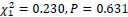 , though both groups showed significant fear recovery even in the CS- condition (Wilcoxon signed rank test, reminder: P = 0.0043, no-reminder: P = 0.0037). Next, we examined the mean SCR for CS- for the 30min, 6h and 24h groups in study 2 and found that there was indeed a group difference (one-way ANOVA,F<sub>2.76</sub> = 5.3462, P = 0.0067, panel b), suggesting that the CS- related SCR was influenced by the test time (30min, 6h or 24h). We also tested the CS- related SCR for the 4 groups in study 3 (where test was conducted 1 hour after the retrieval-extinction training) and found that across TMS stimulation types (PFC vs. VER) and reminder types (reminder vs. no-reminder) the ANOVA analysis did not yield main effect of TMS stimulation type (F<sub>1.71</sub> = 0.322, P = 0.572) nor main effect of reminder type (F<sub>1.71</sub> = 0.0499, P = 0.824, panel c). We added the R-VER group results in study 3 (see panel c) to panel b and plotted the CS- SCR difference across 4 different test time points and found that CS- SCR decreased as the test-extinction delay increased (Jonckheere-Terpstra test, P = 0.00028). These results suggest a natural “forgetting” tendency for CS- related SCR and highlight the importance of having the CS- as a control condition to which the CS+ related SCR was compared with.
Author response image 1.
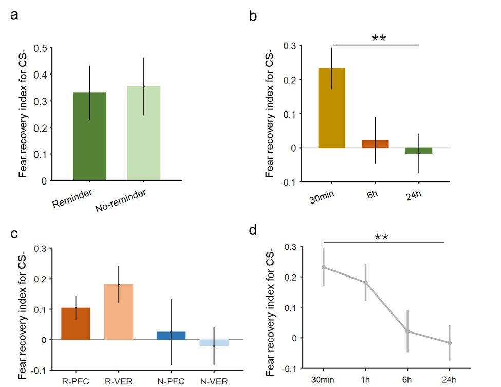
(6D) The 6 hour group was clearly tested at a different time of day compared to the 30 min and 24 hour groups. This could have influenced the SCRs in this group and, thereby, contributed to the pattern of results obtained.
Again, we answered this question in our previous response. Please see the following for our previous response:
For the 30min and 24h groups, the test phase can be arranged in the morning, in the afternoon or at night. However, for the 6h group, the test phase was inevitably in the afternoon or at night since we wanted to exclude the potential influence of night sleep on the expression of fear memory (see Author response table 1 below). If we restricted the test time in the afternoon or at night for all three groups, then the timing of their extinction training was not matched.
Author response table 1.
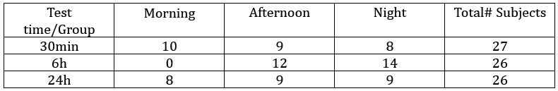
Nevertheless, we also went back and examined the data for the subjects only tested in the afternoon or at nights in the 30min and 24h groups to match with the 6h group where all the subjects were tested either in the afternoon or at night. According to the table above, we have 17 subjects for the 30min group (9+8),18 subjects for the 24h group (9 + 9) and 26 subjects for the 6h group (12 + 14). As Author response image 2 shows, the SCR patterns in the fear acquisition, extinction and test phases were similar to the results presented in the original figure.
Author response image 2.
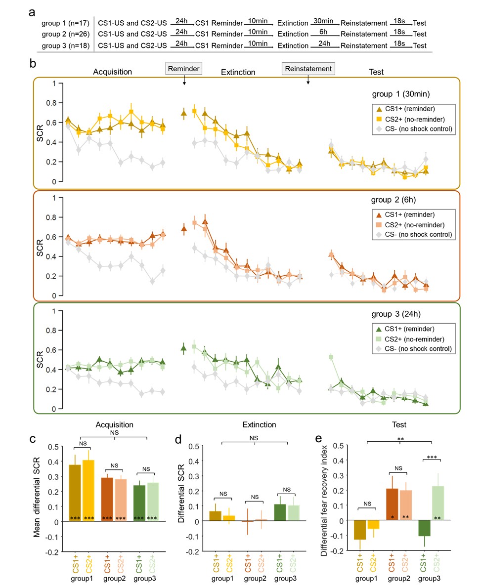
(6E) The authors find different patterns of responses to CS1 and CS2 when they were tested 30 min after extinction versus 24 h after extinction. On this basis, they infer distinct memory update mechanisms. However, I still can't quite see why the different patterns of responses at these two time points after extinction need to be taken to infer different memory update mechanisms. That is, the different patterns of responses at the two time points could be indicative of the same "memory update mechanism" in the sense that the retrieval-extinction procedure induces a short-term memory suppression that serves as the basis for the longer-term memory suppression (i.e., the reconsolidation effect). My pushback on this point is based on the notion of what constitutes a memory update mechanism; and is motivated by what I take to be a rather loose use of language/terminology in the reconsolidation literature and this paper specifically (for examples, see the title of the paper and line 2 of the abstract).
As we mentioned previously, the term “mechanism” might have different connotations for different researchers. We aim to report a novel memory deficit following the retrieval-extinction paradigm, which differed significantly from the purported reconsolidation related long-term fear amnesia in terms of its timescale, cue-specificity and thought-control ability. Further TMS study confirmed that the intact dlPFC function is necessary for the short-term memory deficit. It’s based on these results we proposed that the short-term fear amnesia might be related to a different cognitive “mechanism”. As mentioned above, we now clarify what we mean by “mechanism” in the abstract and introduction (lines 31-34, 97-101).
Reviewer #2 (Public review):
The fear acquisition data is converted to a differential fear SCR and this is what is analysed (early vs late). However, the figure shows the raw SCR values for CS+ and CS- and therefore it is unclear whether acquisition was successful (despite there being an "early" vs "late" effect - no descriptives are provided).
(1) There are still no descriptive statistics to substantiate learning in Experiment 1.
We answered this question in our previous response letter. We are sorry that the definition of “early” and “late” trials was scattered in the manuscript. For example, we wrote “the late phase of acquisition (last 5 trials)” (Line 375-376) in the results section. Since there were 10 trials in total for the acquisition stage, we define the first 5 trials and the last 5 trials as “early” and “late” phases of the acquisition stage and explicitly added them into the first occasion “early” and “late” terms appeared (lines 316-318).
In the results section, we did test whether the acquisition was successful in our previous manuscript (Line 316-325):
“To assess fear acquisition across groups (Figure 1B and C), we conducted a mixed two-way ANOVA of group (reminder vs. no-reminder) x time (early vs. late part of the acquisition; first 5 and last 5 trials, correspondingly) on the differential fear SCR. Our results showed a significant main effect of time (early vs. late; F<sub>1,55</sub> \= 6.545, P \= 0.013, η<sup>2</sup> \= 0.106), suggesting successful fear acquisition in both groups. There was no main effect of group (reminder vs. no-reminder) or the group x time interaction (group: F<sub>1,55</sub> \= 0.057, P \= 0.813, η<sup>2</sup> \= 0.001; interaction: F<sub>1,55</sub> \= 0.066, P \= 0.798, η<sup>2</sup> \= 0.001), indicating similar levels of fear acquisition between two groups. Post-hoc t-tests confirmed that the fear responses to the CS+ were significantly higher than that of CS- during the late part of acquisition phase in both groups (reminder group: t<sub>29</sub> \= 6.642, P < 0.001; no-reminder group: t<sub>26</sub> = 8.522, P < 0.001; Figure 1C). Importantly, the levels of acquisition were equivalent in both groups (early acquisition: t<sub>55</sub> \= -0.063, P \= 0.950; late acquisition: t<sub>55</sub> \= -0.318, P \= 0.751; Figure 1C).”
In Experiment 1 (Test results) it is unclear whether the main conclusion stems from a comparison of the test data relative to the last extinction trial ("we defined the fear recovery index as the SCR difference between the first test trial and the last extinction trial for a specific CS") or the difference relative to the CS- ("differential fear recovery index between CS+ and CS-"). It would help the reader assess the data if Fig 1e presents all the indexes (both CS+ and CS-). In addition, there is one sentence which I could not understand "there is no statistical difference between the differential fear recovery indexes between CS+ in the reminder and no reminder groups (P=0.048)". The p value suggests that there is a difference, yet it is not clear what is being compared here. Critically, any index taken as a difference relative to the CS- can indicate recovery of fear to the CS+ or absence of discrimination relative to the CS-, so ideally the authors would want to directly compare responses to the CS+ in the reminder and no-reminder groups. In the absence of such comparison, little can be concluded, in particular if SCR CS- data is different between groups. The latter issue is particularly relevant in Experiment 2, in which the CS- seems to vary between groups during the test and this can obscure the interpretation of the result.
(2) In the revised analyses, the authors now show that CS- changes in different groups (for example, Experiment 2) so this means that there is little to conclude from the differential scores because these depend on CS-. It is unclear whether the effects arise from CS+ performance or the differential which is subject to CS- variations.
There was a typo in the “P = 0.048” sentence and we have corrected it in our last response letter. Also in the previous response letter, we specifically addressed how the fear recovery index was defined (also in the revised manuscript).
In most of the fear conditioning studies, CS- trials were included as the baseline control. In turn, most of the analyses conducted also involved comparisons between different groups. Directly comparing CS+ trials across groups (or conditions) is rare. In our study 2, we showed that the CS- response decreased as a function of testing delays (30min, 1hr, 6hr and 24hr). Ideally, it would be nice to show that the CS- across groups/conditions did not change. However, even in those circumstances, comparisons are still based on the differential CS response (CS+ minus CS-), that is, the difference of difference. It is also important to note that difference score is important as CS+ alone or across conditions is difficult to interpret, especially in humans, due to noise, signal fluctuations, and irrelevant stimulus features; therefore trials-wise reference is essential to assess the CS+ in the context of a reference stimulus in each trial (after all, the baselines are different). We are listing a few influential papers in the field that the CS- responses were not particularly equivalent across groups/conditions and argue that this is a routine procedure (Kindt & Soeter 2018 Figs. 2-3; Sevenster et al., 2013 Fig. 3; Liu et al., 2014 Fig. 1; Raio et al., 2017 Fig. 2).
In experiment 1, the findings suggest that there is a benefit of retrieval followed by extinction in a short-term reinstatement test. In Experiment 2, the same effect is observed to a cue which did not undergo retrieval before extinction (CS2+), a result that is interpreted as resulting from cue-independence, rather than a failure to replicate in a within-subjects design the observations of Experiment 1 (between-subjects). Although retrieval-induced forgetting is cue-independent (the effect on items that are suppressed [Rp-] can be observed with an independent probe), it is not clear that the current findings are similar, and thus that the strong parallels made are not warranted. Here, both cues have been extinguished and therefore been equally exposed during the critical stage.
(3) The notion that suppression is automatic is speculative at best
We have responded the same question in our previous revision. Please note that our results from study 1 (the comparison between reminder and no-reminder groups) was not set up to test the cue-independence hypothesis for the short-term amnesia with only one CS+. Results from both study 2 (30min condition) and study 3 confirmed the cue-independence hypothesis and therefore we believe interpreting results from study 2 as “a failure to replicate in a within-subject design of the observations of Experiment 1” is not the case.
We agree that the proposal of automatic or unconscious memory suppression is speculative and that’s why we mentioned it in the discussion. The timescale, cue-specificity and the thought-control ability dependence of the short-term fear amnesia identified in our studies was reminiscent of the memory suppression effects reported in the previous literature. However, memory suppression typically adopted a conscious “suppression” treatment (such as the think/no-think paradigm), which was absent in the current study. However, the retrieval-induced forgetting (RIF), which is also considered a memory suppression paradigm via inhibitory control, does not require conscious effort to suppress any particular thought. Based on these results and extant literature, we raised the possibility of memory suppression as a potential mechanism. We make clear in the discussion that the suppression hypothesis and connections with RIF will require further evidence (lines 615-616):
“future research will be needed to investigate whether the short-term effect we observed is specifically related to associative memory or the spontaneous nature of suppression as in RIF (Figure 6C).”
(4) It still struggle with the parallels between these findings and the "limbo" literature. Here you manipulated the retention interval, whereas in the cited studies the number of extinction (exposure) was varied. These are two completely different phenomena.
We borrowed the “limbo” term to stress the transitioning from short-term to long-term memory deficits (the 6hr test group). Merlo et al. (2014) found that memory reconsolidation and extinction were dissociable processes depending on the extent of memory retrieval. They argued that there was a “limbo” transitional state, where neither the reconsolidation nor the extinction process was engaged. Our results suggest that at the test delay of 6hr, neither the short-term nor the long-term effect was present, signaling a “transitional” state after which the short-term memory deficit wanes and the long-term deficit starts to take over. We make this idea more explicit as follows (lines 622-626):
“These works identified important “boundary conditions” of memory retrieval in affecting the retention of the maladaptive emotional memories. In our study, however, we showed that even within a boundary condition previously thought to elicit memory reconsolidation, mnemonic processes other than reconsolidation could also be at work, and these processes jointly shape the persistence of fear memory.”
(5) My point about the data problematic for the reconsolidation (and consolidation) frameworks is that they observed memory in the absence of the brain substrates that are needed for memory to be observed. The answer did not address this. I do not understand how the latent cause model can explain this, if the only difference is the first ITI. Wouldn't participants fail to integrate extinction with acquisition with a longer ITI?
We take the sentence “they observed memory in the absence of the brain substrates that are needed for memory to be observed” as referring to the long-term memory deficit in our study. As we responded before, the aim of this manuscript was not about investigating the brain substrates involved in memory reconsolidation (or consolidation). Using a memory retrieval-extinction paradigm, we discovered a novel short-term memory effect, which differed from the purported reconsolidation effect in terms of timescale, cue-specificity and thought-control ability dependence. We further showed that both memory retrieval and intact dlPFC functions were necessary to observe the short-term memory deficit effect. Therefore, we conclude that the brain mechanism involved in such an effect should be different from the one related to the purported reconsolidation effect. We make this idea more explicit as follows (lines 546-547):
“Therefore, findings of the short-term fear amnesia suggest that the reconsolidation framework falls short to accommodate this more immediate effect (Figure 6A and B).”
Whilst I could access the data in the OFS site, I could not make sense of the Matlab files as there is no signposting indicating what data is being shown in the files. Thus, as it stands, there is no way of independently replicating the analyses reported.
(6) The materials in the OSF site are the same as before, they haven't been updated.
Last time we thought the main issue was the OSF site not being publicly accessible and thus made it open to all visitors. We have added descriptive file to explain the variables to help visitors to replicate the analyses we took.
(7) Concerning supplementary materials, the robustness tests are intended to prove that you 1) can get the same results by varying the statistical models or 2) you can get the same results when you include all participants. Here authors have done both so this does not help. Also, in the rebuttal letter, they stated "Please note we did not include non-learners in these analyses " which contradicts what is stated in the figure captions "(learners + non learners)"
In the supplementary materials, we did the analyses of varying the statistical models and including both learners and non-learners separately, instead of both. In fact, in the supplementary material Figs. 1 & 2, we included all the participants and performed similar analysis as in the main text and found similar results (learners + non-learners). Also, in the text of the supplementary material, we used a different statistical analysis method to only learners (analyzing subjects reported in the main text using a different method) and achieved similar results. We believe this is exactly what the reviewer suggested us to do. Also there seems to be a misunderstanding for the "Please note we did not include non-learners in these analyses" sentence in the rebuttal letter. As the reviewer can see, the full sentence read “Please note we did not include non-learners in these analyses (the texts of the supplementary materials)”. We meant to express that the Figures and texts in the supplementary material reflect two approaches: 1) Figures depicting re-analysis with all the included subjects (learners + non learners); 2) Text describing different analysis with learners. We added clarifications to emphasize these approaches in the supplementary materials.
(8) Finally, the literature suggesting that reconsolidation interference "eliminates" a memory is not substantiated by data nor in line with current theorising, so I invite a revision of these strong claims.
We agree and have toned down the strong claims.
Overall, I conclude that the revised manuscript did not address my main concerns.
In both rounds of responses, we tried our best to address the reviewer’s concerns. We hope that the clarifications in this letter and revisions in the text address the remaining concerns. Thank you for your feedback.
Reference:
Kindt, M. and Soeter, M. 2018. Pharmacologically induced amnesia for learned fear is time and sleep dependent. Nat Commun, 9, 1316.
Liu, J., Zhao, L., Xue, Y., Shi, J., Suo, L., Luo, Y., Chai, B., Yang, C., Fang, Q., Zhang, Y., Bao, Y., Pickens, C. L. and Lu, L. 2014. An unconditioned stimulus retrieval extinction procedure to prevent the return of fear memory. Biol Psychiatry, 76, 895-901.
Raio, C. M., Hartley, C. A., Orederu, T. A., Li, J. and Phelps, E. A. 2017. Stress attenuates the flexible updating of aversive value. Proc Natl Acad Sci U S A, 114, 11241-11246.
Sevenster, D., Beckers, T., & Kindt, M. 2013. Prediction error governs pharmacologically induced amnesia for learned fear. Science (New York, N.Y.), 339(6121), 830–833.
Author response:
The following is the authors’ response to the current reviews.
eLife Assessment<br /> This study offers valuable insights into how humans detect and adapt to regime shifts, highlighting distinct contributions of the frontoparietal network and ventromedial prefrontal cortex to sensitivity to signal diagnosticity and transition probabilities. The combination of an innovative task design, behavioral modeling, and model-based fMRI analyses provides a solid foundation for the conclusions; however, the neuroimaging results have several limitations, particularly a potential confound between the posterior probability of a switch and the passage of time that may not be fully controlled by including trial number as a regressor. The control experiments intended to address this issue also appear conceptually inconsistent and, at the behavioral level, while informing participants of conditional probabilities rather than requiring learning is theoretically elegant, such information is difficult to apply accurately, as shown by well-documented challenges with conditional reasoning and base-rate neglect. Expressing these probabilities as natural frequencies rather than percentages may have improved comprehension. Overall, the study advances understanding of belief updating under uncertainty but would benefit from more intuitive probabilistic framing and stronger control of temporal confounds in future work.
We thank the editors for the assessment. The editor added several limitations based on the new reviewer 3 in this round, which we address below.
With regard to temporal confounds, we clarified in the main text and response to Reviewer 3 that we had already addressed the potential confound between posterior probability of a switch and passage of time in GLM-2 with the inclusion of intertemporal prior. After adding intertemporal prior in the GLM, we still observed the same fMRI results on probability estimates. In addition, we did two other robustness checks, which we mentioned in the manuscript.
With regard to response mode (probability estimation rather than choice or indicating natural frequencies), we wish to point out that the in previous research by Massey and Wu (2005), which the current study was based on, the concern of participants showing system-neglect tendencies due to the mode of information delivery, namely indicating beliefs through reporting probability estimates rather than through choice or other response mode was addressed. Massy and Wu (2005, Study 3) found the same biases when participants performed a choice task that did not require them to indicate probability estimates.
With regard to the control experiments, the control experiments in fact were not intended to address the confounds between posterior probability and passage of time. Rather, they aimed to address whether the neural findings were unique to change detection (Experiment 2) and to address visual and motor confounds (Experiment 3). These and the results of the control experiments were mentioned on page 18-19.
Finally, we wish to highlight that we had performed detailed model comparisons after reviewer 2’s suggestions. Although reviewer 2 was unable to re-review the manuscript, we believe this provides insight into the literature on change detection. See “Incorporating signal dependency into system-neglect model led to better models for regime-shift detection” (p.27-30). The model comparison showed that system-neglect models that incorporate signal dependency are better models than the original system-neglect model in describing participants probability estimates. This suggests that people respond to change-consistent and change-inconsistent signals differently when judging whether the regime had changed. This was not reported in previous behavioral studies and was largely inspired by the neural finding on signal dependency in the frontoparietal cortex. It indicates that neural findings can provide novel insights into computational modeling of behavior.
Public Reviews:
Reviewer #1 (Public review):
Summary:
The study examines human biases in a regime-change task, in which participants have to report the probability of a regime change in the face of noisy data. The behavioral results indicate that humans display systematic biases, in particular, overreaction in stable but noisy environments and underreaction in volatile settings with more certain signals. fMRI results suggest that a frontoparietal brain network is selectively involved in representing subjective sensitivity to noise, while the vmPFC selectively represents sensitivity to the rate of change.
Strengths:
- The study relies on a task that measures regime-change detection primarily based on descriptive information about the noisiness and rate of change. This distinguishes the study from prior work using reversal-learning or change-point tasks in which participants are required to learn these parameters from experiences. The authors discuss these differences comprehensively.
- The study uses a simple Bayes-optimal model combined with model fitting, which seems to describe the data well. The model is comprehensively validated.
- The authors apply model-based fMRI analyses that provide a close link to behavioral results, offering an elegant way to examine individual biases.
We thank the reviewer for the comments.
Weaknesses:
The authors have adequately addressed most of my prior concerns.
We thank the reviewer for recognizing our effort in addressing your concerns.
My only remaining comment concerns the z-test of the correlations. I agree with the non-parametric test based on bootstrapping at the subject level, providing evidence for significant differences in correlations within the left IFG and IPS.
However, the parametric test seems inadequate to me. The equation presented is described as the Fisher z-test, but the numerator uses the raw correlation coefficients (r) rather than the Fisher-transformed values (z). To my understanding, the subtraction should involve the Fisher z-scores, not the raw correlations.
More importantly, the Fisher z-test in its standard form assumes that the correlations come from independent samples, as reflected in the denominator (which uses the n of each independent sample). However, in my opinion, the two correlations are not independent but computed within-subject. In such cases, parametric tests should take into account the dependency. I believe one appropriate method for the current case (correlated correlation coefficients sharing a variable [behavioral slope]) is explained here:
Meng, X.-l., Rosenthal, R., & Rubin, D. B. (1992). Comparing correlated correlation coefficients. Psychological Bulletin, 111(1), 172-175. https://doi.org/10.1037/0033-2909.111.1.172
It should be implemented here:
Diedenhofen B, Musch J (2015) cocor: A Comprehensive Solution for the Statistical Comparison of Correlations. PLoS ONE 10(4): e0121945. https://doi.org/10.1371/journal.pone.0121945
My recommendation is to verify whether my assumptions hold, and if so, perform a test that takes correlated correlations into account. Or, to focus exclusively on the non-parametric test.
In any case, I recommend a short discussion of these findings and how the authors interpret that some of the differences in correlations are not significant.
Thank you for the careful check. Yes. This was indeed a mistake from us. We also agree that the two correlations are not independent. Therefore, we modified the test that accounts for dependent correlations by following Meng et al. (1992) suggested by the reviewer.
We referred to the correlation between neural and behavioral sensitivity at change-consistent (blue) signals as , and that at change-inconsistent (red) signals as 𝑟<sub>𝑟𝑒𝑑</sub>. To statistically compare these two correlations, we adopted the approach of Meng et al. (1992), which specifically tests differences between dependent correlations according to the following equation
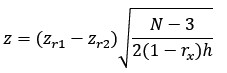
where is the number of subjects, 𝑧<sub>𝑟𝑖</sub> is the Fisher z-transformed value of 𝑟<sub>𝑖</sub>, 𝑟<sub>1</sub> = 𝑟<sub>𝑏𝑙𝑢𝑒</sub> and 𝑟<sub>2</sub> = 𝑟<sub>𝑟𝑒𝑑</sub>. 𝑟<sub>𝑥</sub> is the correlation between the neural sensitivity at change-consistent signals and change-inconsistent signals.
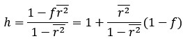
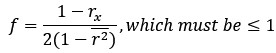
Where  is the mean of the
 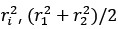 , and 𝑓 should be set to 1 if > 1.
We found that among the five ROIs in the frontoparietal network, two of them, namely the left IFG and left IPS, the difference in correlation was significant (one-tailed z test; left IFG: 𝑧 = 1.8908, 𝑝 = 0.0293; left IPS: 𝑧 = 2.2584, 𝑝 = 0.0049). For the remaining three ROIs, the difference in correlation was not significant (dmPFC: 𝑧 = 0.9522, 𝑝 = 0.1705; right IFG: 𝑧 = 0.9860, 𝑝 = 0.1621; right IPS: 𝑧 = 1.4833, 𝑝 = 0.0690). We chose one-tailed test because we already know the correlation under the blue signals was significantly greater than 0. These updated results are consistent with the nonparametric tests we had already performed and we will update them in the revised manuscript.
Reviewer #3 (Public review):
This study concerns how observers (human participants) detect changes in the statistics of their environment, termed regime shifts. To make this concrete, a series of 10 balls are drawn from an urn that contains mainly red or mainly blue balls. If there is a regime shift, the urn is changed over (from mainly red to mainly blue) at some point in the 10 trials. Participants report their belief that there has been a regime shift as a % probability. Their judgement should (mathematically) depend on the prior probability of a regime shift (which is set at one of three levels) and the strength of evidence (also one of three levels, operationalized as the proportion of red balls in the mostly-blue urn and vice versa). Participants are directly instructed of the prior probability of regime shift and proportion of red balls, which are presented on-screen as numerical probabilities. The task therefore differs from most previous work on this question in that probabilities are instructed rather than learned by observation, and beliefs are reported as numerical probabilities rather than being inferred from participants' choice behaviour (as in many bandit tasks, such as Behrens 2007 Nature Neurosci).
The key behavioural finding is that participants over-estimate the prior probability of regime change when it is low, and under estimate it when it is high; and participants over-estimate the strength of evidence when it is low and under-estimate it when it is high. In other words participants make much less distinction between the different generative environments than an optimal observer would. This is termed 'system neglect'. A neuroeconomic-style mathematical model is presented and fit to data.
Functional MRI results how that strength of evidence for a regime shift (roughly, the surprise associated with a blue ball from an apparently red urn) is associated with activity in the frontal-parietal orienting network. Meanwhile, at time-points where the probability of a regime shift is high, there is activity in another network including vmPFC. Both networks show individual differences effects, such that people who were more sensitive to strength of evidence and prior probability show more activity in the frontal-parietal and vmPFC-linked networks respectively.
We thank the reviewer for the overall descriptions of the manuscript.
Strengths:
(1) The study provides a different task for looking at change-detection and how this depends on estimates of environmental volatility and sensory evidence strength, in which participants are directly and precisely informed of the environmental volatility and sensory evidence strength rather than inferring them through observation as in most previous studies
(2) Participants directly provide belief estimates as probabilities rather than experimenters inferring them from choice behaviour as in most previous studies<br /> (3) The results are consistent with well-established findings that surprising sensory events activate the frontal-parietal orienting network whilst updating of beliefs about the word ('regime shift') activates vmPFC.
Thank you for these assessments.
Weaknesses:
(1) The use of numerical probabilities (both to describe the environments to participants, and for participants to report their beliefs) may be problematic because people are notoriously bad at interpreting probabilities presented in this way, and show poor ability to reason with this information (see Kahneman's classic work on probabilistic reasoning, and how it can be improved by using natural frequencies). Therefore the fact that, in the present study, people do not fully use this information, or use it inaccurately, may reflect the mode of information delivery.
We appreciate the reviewer’s concern on this issue. The concern was addressed in Massey and Wu (2005) as participants performed a choice task in which they were not asked to provide probability estimates (Study 3 in Massy and Wu, 2005). Instead, participants in Study 3 were asked to predict the color of the ball before seeing a signal. This was a more intuitive way of indicating his or her belief about regime shift. The results from the choice task were identical to those found in the probability estimation task (Study 1 in Massey and Wu). We take this as evidence that the system-neglect behavior the participants showed was less likely to be due to the mode of information delivery.
(2) Although a very precise model of 'system neglect' is presented, many other models could fit the data.
For example, you would get similar effects due to attraction of parameter estimates towards a global mean - essentially application of a hyper-prior in which the parameters applied by each participant in each block are attracted towards the experiment-wise mean values of these parameters. For example, the prior probability of regime shift ground-truth values [0.01, 0.05, 0.10] are mapped to subjective values of [0.037, 0.052, 0.069]; this would occur if observers apply a hyper-prior that the probability of regime shift is about 0.05 (the average value over all blocks). This 'attraction to the mean' is a well-established phenomenon and cannot be ruled out with the current data (I suppose you could rule it out by comparing to another dataset in which the mean ground-truth value was different).
We thank the reviewer for this comment. It is true that the system-neglect model is not entirely inconsistent with regression to the mean, regardless of whether the implementation has a hyper prior or not. In fact, our behavioral measure of sensitivity to transition probability and signal diagnosticity, which we termed the behavioral slope, is based on linear regression analysis. In general, the modeling approach in this paper is to start from a generative model that defines ideal performance and consider modifying the generative model when systematic deviations in actual performance from the ideal is observed. In this approach, a generative model with hyper-prior would be more complex to begin with, and a regression to the mean idea by itself does not generate a priori predictions.
More generally, any model in which participants don't fully use the numerical information they were given would produce apparent 'system neglect'. Four qualitatively different example reasons are: 1. Some individual participants completely ignored the probability values given. 2. Participants did not ignore the probability values given, but combined them with a hyperprior as above. 3. Participants had a reporting bias where their reported beliefs that a regime-change had occurred tend to be shifted towards 50% (rather than reporting 'confident' values such 5% or 95%). 4. Participants underweighted probability outliers resulting in underweighting of evidence in the 'high signal diagnosticity' environment (10.1016/j.neuron.2014.01.020 )
In summary I agree that any model that fits the data would have to capture the idea that participants don't differentiate between the different environments as much as they should, but I think there are a number of qualitatively different reasons why they might do this - of which the above are only examples - hence I find it problematic that the authors present the behaviour as evidence for one extremely specific model.
Thank you for raising this point. The modeling principle we adopt is the following. We start from the normative model—the Bayesian model—that defined what normative behavior should look like. We compared participants’ behavior with the Bayesian model and found systematic deviations from it. To explain those systematic deviations, we considered modeling options within the confines of the same modeling framework. In other words, we considered a parameterized version of the Bayesian model, which is the system-neglect model and examined through model comparison the best modeling choice. This modeling approach is not uncommon, and many would agree this is the standard approach in economics and psychology. For example, Kahneman and Tversky adopted this approach when proposing prospect theory, a modification of expected utility theory where expected utility theory can be seen as one specific model for how utility of an option should be computed.
(3) Despite efforts to control confounds in the fMRI study, including two control experiments, I think some confounds remain.
For example, a network of regions is presented as correlating with the cumulative probability that there has been a regime shift in this block of 10 samples (Pt). However, regardless of the exact samples shown, doesn't Pt always increase with sample number (as by the time of later samples, there have been more opportunities for a regime shift)? Unless this is completely linear, the effect won't be controlled by including trial number as a co-regressor (which was done).
Thank you for raising this concern. Yes, Pt always increases with sample number regardless of evidence (seeing change-consistent or change-inconsistent signals). This is captured by the ‘intertemporal prior’ in the Bayesian model, which we included as a regressor in our GLM analysis (GLM-2), in addition to Pt. In short, GLM-1 had Pt and sample number. GLM-2 had Pt, intertemporal prior, and sample number, among other regressors. And we found that, in both GLM-1 and GLM-2, both vmPFC and ventral striatum correlated with Pt.
To make this clearer, we updated the main text to further clarify this on p.18:
On the other hand, two additional fMRI experiments are done as control experiments and the effect of Pt in the main study is compared to Pt in these control experiments. Whilst I admire the effort in carrying out control studies, I can't understand how these particular experiment are useful controls. For example in experiment 3 participants simply type in numbers presented on the screen - how can we even have an estimate of Pt from this task?
We thank the reviewer for this comment. The purpose of Experiment 3 was to control for visual and motor confounds. In other words, if subjects saw the similar visual layout and were just instructed to press numbers, would we observe the vmPFC, ventral striatum, and the frontoparietal network like what we did in the main experiment (Experiment 1)?
The purpose of Experiment 2 was to establish whether what we found about Pt was unique to change detection. In Experiment 2, subjects estimated the probability that the current regime is the blue regime (just as they did in Experiment 1) except that there were no regime shifts involved. In other words, it is possible that the regions we identified were generally associated with probability estimation and not particularly about change detection. And we used Experiment 2 to examine whether this were true.
(4) The Discussion is very long, and whilst a lot of related literature is cited, I found it hard to pin down within the discussion, what the key contributions of this study are. In my opinion it would be better to have a short but incisive discussion highlighting the advances in understanding that arise from the current study, rather than reviewing the field so broadly.
Thank you. We received different feedbacks from previous reviews on what to include in Discussion. To address the reviewer’s concern, we will revise the Discussion to better highlight the key contributions of the current study at the beginning of Discussion.
Recommendations for the authors:
Reviewer #3 (Recommendations for the authors):
Many of the figures are too tiny - the writing is very small, as are the pictures of brains. I'd suggest adjusting these so they will be readable without enlarging.
Thank you. We will enlarge the figures to make them more readable.
The following is the authors’ response to the original reviews.
Public Reviews:
Reviewer #1 (Public review):
Summary:
The study examines human biases in a regime-change task, in which participants have to report the probability of a regime change in the face of noisy data. The behavioral results indicate that humans display systematic biases, in particular, overreaction in stable but noisy environments and underreaction in volatile settings with more certain signals. fMRI results suggest that a frontoparietal brain network is selectively involved in representing subjective sensitivity to noise, while the vmPFC selectively represents sensitivity to the rate of change.
Strengths:
(1) The study relies on a task that measures regime-change detection primarily based on descriptive information about the noisiness and rate of change. This distinguishes the study from prior work using reversal-learning or change-point tasks in which participants are required to learn these parameters from experiences. The authors discuss these differences comprehensively.
Thank you for recognizing our contribution to the regime-change detection literature and our effort in discussing our findings in relation to the experience-based paradigms.
(2) The study uses a simple Bayes-optimal model combined with model fitting, which seems to describe the data well.
Thank you for recognizing the contribution of our Bayesian framework and systemneglect model.
(3) The authors apply model-based fMRI analyses that provide a close link to behavioral results, offering an elegant way to examine individual biases.
Thank you for recognizing our execution of model-based fMRI analyses and effort in using those analyses to link with behavioral biases.
Weaknesses:
My major concern is about the correlational analysis in the section "Under- and overreactions are associated with selectivity and sensitivity of neural responses to system parameters", shown in Figures 5c and d (and similarly in Figure 6). The authors argue that a frontoparietal network selectively represents sensitivity to signal diagnosticity, while the vmPFC selectively represents transition probabilities. This claim is based on separate correlational analyses for red and blue across different brain areas. The authors interpret the finding of a significant correlation in one case (blue) and an insignificant correlation (red) as evidence of a difference in correlations (between blue and red) but don't test this directly. This has been referred to as the "interaction fallacy" (Niewenhuis et al., 2011; Makin & Orban de Xivry 2019). Not directly testing the difference in correlations (but only the differences to zero for each case) can lead to wrong conclusions. For example, in Figure 5c, the correlation for red is r = 0.32 (not significantly different from zero) and r = 0.48 (different from zero). However, the difference between the two is 0.1, and it is likely that this difference itself is not significant. From a statistical perspective, this corresponds to an interaction effect that has to be tested directly. It is my understanding that analyses in Figure 6 follow the same approach.
Relevant literature on this point is:
Nieuwenhuis, S, Forstmann, B & Wagenmakers, EJ (2011). Erroneous analyses of interactions in neuroscience: a problem of significance. Nat Neurosci 14, 11051107. https://doi.org/10.1038/nn.2886
Makin TR, Orban de Xivry, JJ (2019). Science Forum: Ten common statistical mistakes to watch out for when writing or reviewing a manuscript. eLife 8:e48175. https://doi.org/10.7554/eLife.48175
There is also a blog post on simulation-based comparisons, which the authors could check out: https://garstats.wordpress.com/2017/03/01/comp2dcorr/
I recommend that the authors carefully consider what approach works best for their purposes. It is sometimes recommended to directly compare correlations based on Monte-Carlo simulations (cf Makin & Orban). It might also be appropriate to run a regression with the dependent variable brain activity (Y) and predictors brain area (X) and the model-based term of interest (Z). In this case, they could include an interaction term in the model:
Y = \beta_0 + \beta_1 \cdot X + \beta_2 \cdot Z + \beta_3 \cdot X \cdot Z
The interaction term reflects if the relationship between the model term Z and brain activity Y is conditional on the brain area of interest X.
Thank you for the suggestion. In response, we tested for the difference in correlation both parametrically and nonparametrically. The results were identical. In the parametric test, we used the Fisher z transformation to transform the difference in correlation coefficients to the z statistic. That is, for two correlation coefficients, 𝑟<sub>1</sub> (with sample size 𝑛<sub>1</sub>) and 𝑟<sub>2</sub>, (with sample size 𝑛<sub>2</sub>), the z statistic of the difference in correlation is given by
We referred to the correlation between neural and behavioral sensitivity at change-consistent (blue) signals as 𝑟<sub>𝑏𝑙𝑢𝑒</sub>, and that at change-inconsistent (red) signals as 𝑟<sub>𝑟𝑒𝑑</sub>. For the Fisher z transformation 𝑟<sub>1</sub>= 𝑟<sub>𝑏𝑙𝑢𝑒</sub> and 𝑟<sub>2</sub> \= 𝑟<sub>𝑟𝑒𝑑</sub>. We found that among the five ROIs in the frontoparietal network, two of them, namely the left IFG and left IPS, the difference in correlation was significant (one-tailed z test; left IFG: 𝑧 = 1.8355, 𝑝 =0.0332; left IPS: 𝑧 = 2.3782, 𝑝 = 0.0087). For the remaining three ROIs, the difference in correlation was not significant (dmPFC: 𝑧 = 0.7594, 𝑝 = 0.2238; right IFG: 𝑧 = 0.9068, 𝑝 = 0.1822; right IPS: 𝑧 = 1.3764, 𝑝 = 0.0843). We chose one-tailed test because we already know the correlation under the blue signals was significantly greater than 0.
In the nonparametric test, we performed nonparametric bootstrapping to test for the difference in correlation (Efron & Tibshirani, 1994). We resampled with replacement the dataset (subject-wise) and used the resampled dataset to compute the difference in correlation. We then repeated the above for 100,000 times so as to estimate the distribution of the difference in correlation coefficients, tested for significance and estimated p-value based on this distribution. Consistent with our parametric tests, here we also found that the difference in correlation was significant in left IFG and left IPS (left IFG: 𝑟<sub>𝑏𝑙𝑢𝑒</sub> − 𝑟<sub>𝑟𝑒𝑑</sub> \= 0.46, 𝑝 = 0.0496; left IPS: 𝑟<sub>𝑏𝑙𝑢𝑒</sub> − 𝑟<sub>𝑟𝑒𝑑</sub> \= 0.5306, 𝑝 = 0.0041), but was not significant in dmPFC, right IFG, and right IPS (dmPFC: 𝑟<sub>𝑏𝑙𝑢𝑒</sub> − 𝑟<sub>𝑟𝑒𝑑</sub> \= 0.1634, 𝑝 = 0.1919; right IFG: 𝑟<sub>𝑏𝑙𝑢𝑒</sub> − 𝑟<sub>𝑟𝑒𝑑</sub> \= 0.2123, 𝑝 = 0.1681; right IPS: 𝑟<sub>𝑏𝑙𝑢𝑒</sub> − 𝑟<sub>𝑟𝑒𝑑</sub> \= 0.3434, 𝑝 = 0.0631).
In summary, we found that neural sensitivity to signal diagnosticity in the frontoparietal network measured at change-consistent signals significantly correlated with individual subjects’ behavioral sensitivity to signal diagnosticity (𝑟<sub>𝑏𝑙𝑢𝑒</sub>). By contrast, neural sensitivity to signal diagnosticity measured at change-inconsistent did not significantly correlate with behavioral sensitivity (𝑟<sub>𝑟𝑒𝑑</sub>). The difference in correlation, 𝑟<sub>𝑏𝑙𝑢𝑒</sub> − 𝑟<sub>𝑟𝑒𝑑</sub>, however, was statistically significant in some (left IPS and left IFG) but not all brain regions within the frontoparietal network.
To incorporate these updates, we added descriptions of the methods and results in the revised manuscript. In the Results section (p.26-27):
“We further tested, for each brain region, whether the difference in correlation was significant using both parametric and nonparametric tests (see Parametric and nonparametric tests for difference in correlation coefficients in Methods). The results were identical. In the parametric test, we used the Fisher 𝑧 transformation to transform the difference in correlation coefficients to the 𝑧 statistic. We found that among the five ROIs in the frontoparietal network, two of them, namely the left IFG and left IPS, the difference in correlation was significant (one-tailed z test; left IFG: 𝑧 = 1.8355, 𝑝 = 0.0332; left IPS: 𝑧 = 2.3782, 𝑝 = 0.0087). For the remaining three ROIs, the difference in correlation was not significant (dmPFC: 𝑧 = 0.7594, 𝑝 = 0.2238; right IFG: 𝑧 = 0.9068, 𝑝 = 0.1822; right IPS: 𝑧 = 1.3764, 𝑝 = 0.0843). We chose one-tailed test because we already know the correlation under change-consistent signals was significantly greater than 0. In the nonparametric test, we performed nonparametric bootstrapping to test for the difference in correlation. We referred to the correlation between neural and behavioral sensitivity at change-consistent (blue) signals as 𝑟<sub>𝑏𝑙𝑢𝑒</sub>, and that at change-inconsistent (red) signals as 𝑟<sub>𝑟𝑒𝑑</sub>. Consistent with the parametric tests, we also found that the difference in correlation was significant in left IFG and left IPS (left IFG: 𝑟<sub>𝑏𝑙𝑢𝑒</sub> − 𝑟<sub>𝑟𝑒𝑑</sub> \= 0.46, 𝑝 = 0.0496; left IPS: 𝑟<sub>𝑏𝑙𝑢𝑒</sub> − 𝑟<sub>𝑟𝑒𝑑</sub> \= 0.5306, 𝑝 = 0.0041), but was not significant in dmPFC, right IFG, and right IPS (dmPFC: 𝑟<sub>𝑏𝑙𝑢𝑒</sub> − 𝑟<sub>𝑟𝑒𝑑</sub> \=0.1634, 𝑝 = 0.1919; right IFG: 𝑟<sub>𝑏𝑙𝑢𝑒</sub> − 𝑟<sub>𝑟𝑒𝑑</sub> \= 0.2123, 𝑝 = 0.1681; right IPS: 𝑟<sub>𝑏𝑙𝑢𝑒</sub> − 𝑟<sub>𝑟𝑒𝑑</sub> \= 0.3434, 𝑝 = 0.0631). In summary, we found that neural sensitivity to signal diagnosticity measured at change-consistent signals significantly correlated with individual subjects’ behavioral sensitivity to signal diagnosticity. By contrast, neural sensitivity to signal diagnosticity measured at change-inconsistent signals did not significantly correlate with behavioral sensitivity. The difference in correlation, however, was statistically significant in some (left IPS and left IFG) but not all brain regions within the frontoparietal network.”
In the Methods section, we added on p.53:
“Parametric and nonparametric tests for difference in correlation coefficients. We implemented both parametric and nonparametric tests to examine whether the difference in Pearson correlation coefficients was significant. In the parametric test, we used the Fisher 𝑧 transformation to transform the difference in correlation coefficients to the 𝑧 statistic. That is, for two correlation coefficients, 𝑟<sub>1</sub> (with sample size 𝑛<sub>2</sub>) and 𝑟<sub>2</sub>, (with sample size 𝑛<sub>1</sub>), the 𝑧 statistic of the difference in correlation is given by
We referred to the correlation between neural and behavioral sensitivity at changeconsistent (blue balls) signals as 𝑟<sub>𝑏𝑙𝑢𝑒</sub>, and that at change-inconsistent (red balls) signals as 𝑟<sub>𝑟𝑒𝑑</sub>. For the Fisher 𝑧 transformation, 𝑟<sub>1</sub> \= 𝑟 𝑟<sub>𝑏𝑙𝑢𝑒</sub> and 𝑟<sub>2</sub> \= 𝑟<sub>𝑟𝑒𝑑</sub>. In the nonparametric test, we performed nonparametric bootstrapping to test for the difference in correlation (Efron & Tibshirani, 1994). That is, we resampled with replacement the dataset (subject-wise) and used the resampled dataset to compute the difference in correlation. We then repeated the above for 100,000 times so as to estimate the distribution of the difference in correlation coefficients, tested for significance and estimated p-value based on this distribution.”
Another potential concern is that some important details about the parameter estimation for the system-neglect model are missing. In the respective section in the methods, the authors mention a nonlinear regression using Matlab's "fitnlm" function, but it remains unclear how the model was parameterized exactly. In particular, what are the properties of this nonlinear function, and what are the assumptions about the subject's motor noise? I could imagine that by using the inbuild function, the assumption was that residuals are Gaussian and homoscedastic, but it is possible that the assumption of homoscedasticity is violated, and residuals are systematically larger around p=0.5 compared to p=0 and p=1. Relatedly, in the parameter recovery analyses, the authors assume different levels of motor noise. Are these values representative of empirical values?
We thank the reviewer for this excellent point. The reviewer touched on model parameterization, assumption of noise, and parameter recovery analysis. We answered these questions point-by-point below.
On how our model was parameterized
We parameterized the model according to the system-neglect model in Eq. (2) and estimated the alpha parameter separately for each level of transition probability and the beta parameter separately for each level of signal diagnosticity. As a result, we had a total of 6 parameters (3 alpha and 3 beta parameters) in the model. The system-neglect model is then called by fitnlm so that these parameters can be estimated. The term ‘nonlinear’ regression in fitnlm refers to the fact that you can specify any model (in our case the system-neglect model) and estimate its parameters when calling this function. In our use of fitnlm, we assume that the noise is Gaussian and homoscedastic (the default option).
On the assumptions about subject’s motor noise
We actually never called the noise ‘motor’ because it can be estimation noise as well. In the context of fitnlm, we assume that the noise is Gaussian and homoscedastic.
On the possibility that homoscedasticity is violated
We take the reviewer’s point. In response, we separately estimated the residual standard deviation at different probability intervals ([0.0–0.2), [0.2–0.4), [0.4–0.6), [0.6– 0.8), and [0.8–1.0]). The result is shown in the figure below. The black data points are the average residual standard deviation (across subjects) and the error bars are the standard error of the mean. The residual standard deviation is indeed heteroscedastic— smallest at 0.1 probability and increasing as probability increases and asymptote at 0.5 (Fig. S4).
To examine how this would affect model fitting (parameter estimation), we performed parameter recovery analysis based on these empirically estimated, probabilitydependent residual standard deviation. That is, we simulated subjects’ probability estimates using the system-neglect model and added the heteroscedastic noise according to the empirical values and then estimated the parameter estimates of the system-neglect model. The recovered parameter estimates did not seem to be affected by the heteroscedasticity of the variance. The parameter recovery results were identical to the parameter recovery results when homoscedasticity was assumed. This suggested that although homoscedasticity was violated, it did not affect the accuracy of the parameter estimates (Fig.S4).
We added a section ‘Impact of noise homoscedasticity on parameter estimation’ in Methods section (p.47-48) and a figure in the supplement (Fig. S4) to describe this:
On whether the noise levels in parameter recovery analysis are representative of empirical values
To address the reviewer’s question, we conducted a new analysis using maximum likelihood estimation to simultaneously estimate the system-neglect model and the noise level of each individual subject. To estimate each subject’s noise level, we incorporated a noise parameter into the system-neglect model. We assumed that probability estimates are noisy and modeled them with a Gaussian distribution where the noise parameter (𝜎,-./&) is the standard deviation. At each period, a probability estimate of regime shift was computed according to the system-neglect model where Θ is the set of parameters including parameters in the system-neglect model and the noise parameter. The likelihood function, 𝐿(Θ), is the probability of observing the subject’s actual probability estimate at period 𝑡, 𝑝), given Θ, 𝐿(Θ) = 𝑃(𝑝)|Θ). Since we modeled the noisy probability estimates with a Gaussian distribution, we can therefore express 𝐿(Θ) as 𝐿(Θ)~𝑁(𝑝); 𝑝)*+, 𝜎,-./&) where 𝑝)*+ is the probability estimate predicted by the system-neglect (SN) model at period 𝑡. As a reminder, we referred to a ‘period’ as the time when a new signal appeared during a trial (for a given transition probability and signal diagnosticity). To find that maximum likelihood estimates of ΘMLE, we summed over all periods the negative natural logarithm of likelihood and used MATLAB’s fmincon function to find ΘMLE. Across subjects, we found that the mean noise estimate was 0.1735 and ranged from 0.1118 to 0.2704 (Supplementary Figure S3).”
Compared with our original parameter recovery analysis where the maximum noise level was set at 0.1, our data indicated that some subjects’ noise was larger than this value. Therefore, we expanded our parameter recovery analysis to include noise levels beyond 0.1 to up to 0.3. The results are now updated in Supplementary Fig. S3.
We updated the parameter recovery section (p. 47) in Methods:
The main study is based on N=30 subjects, as are the two control studies. Since this work is about individual differences (in particular w.r.t. to neural representations of noise and transition probabilities in the frontoparietal network and the vmPFC), I'm wondering how robust the results are. Is it likely that the results would replicate with a larger number of subjects? Can the two control studies be leveraged to address this concern to some extent?
We can address the issue of robustness through looking at the effect size. In particular, with respect to individual differences in neural sensitivity of transition probability and signal diagnosticity, since the significant correlation coefficients between neural and behavioral sensitivity were between 0.4 and 0.58 for signal diagnosticity in frontoparietal network (Fig. 5C), and -0.38 and -0.37 for transition probability in vmPFC (Fig. 5D), the effect size of these correlation coefficients was considered medium to large (Cohen, 1992).
It would be challenging to use the control studies to address the robustness concern. The two control studies did not allow us to examine individual differences – in particular with respect to neural selectivity of noise and transition probability – and therefore we think it is less likely to leverage the control studies. Having said that, it is possible to look at neural selectivity of noise (signal diagnosticity) in the first control experiment where subjects estimated the probability of blue regime in a task where there was no regime change (transition probability was 0). However, the fact that there were no regime shifts changed the nature of the task. Instead of always starting at the Red regime in the main experiment, in the first control experiment we randomly picked the regime to draw the signals from. It also changed the meaning and the dynamics of the signals (red and blue) that would appear. In the main experiment the blue signal is a signal consistent with change, but in the control experiment this is no longer the case. In the main experiment, the frequency of blue signals is contingent upon both noise and transition probability. In general, blue signals are less frequent than red signals because of small transition probabilities. But in the first control experiment, the frequency of blue signals may not be less frequent because the regime was blue in half of the trials. Due to these differences, we do not see how analyzing the control experiments could help in establishing robustness because we do not have a good prediction as to whether and how the neural selectivity would be impacted by these differences.
It seems that the authors have not counterbalanced the colors and that subjects always reported the probability of the blue regime. If so, I'm wondering why this was not counterbalanced.
We are aware of the reviewer’s concern. The first reason we did not do these (color counterbalancing and report blue/red regime balancing) was to not confuse the subjects in an already complicated task. Balancing these two variables also comes at the cost of sample size, which was the second reason we did not do it. Although we can elect to do these balancing at the between-subject level to not impact the task complexity, we could have introduced another confound that is the individual differences in how people respond to these variables. This is the third reason we were hesitant to do these counterbalancing.
Reviewer #2 (Public review):
Summary:
This paper focuses on understanding the behavioral and neural basis of regime shift detection, a common yet hard problem that people encounter in an uncertain world.
Using a regime-shift task, the authors examined cognitive factors influencing belief updates by manipulating signal diagnosticity and environmental volatility. Behaviorally, they have found that people demonstrate both over and under-reaction to changes given different combinations of task parameters, which can be explained by a unified system-neglect account. Neurally, the authors have found that the vmPFC-striatum network represents current belief as well as belief revision unique to the regime detection task. Meanwhile, the frontoparietal network represents cognitive factors influencing regime detection i.e., the strength of the evidence in support of the regime shift and the intertemporal belief probability. The authors further link behavioral signatures of system neglect with neural signals and have found dissociable patterns, with the frontoparietal network representing sensitivity to signal diagnosticity when the observation is consistent with regime shift and vmPFC representing environmental volatility, respectively. Together, these results shed light on the neural basis of regime shift detection especially the neural correlates of bias in belief update that can be observed behaviorally.
Strengths:
(1) The regime-shift detection task offers a solid ground to examine regime-shift detection without the potential confounding impact of learning and reward. Relatedly, the system-neglect modeling framework provides a unified account for both over or under-reacting to environmental changes, allowing researchers to extract a single parameter reflecting people's sensitivity to changes in decision variables and making it desirable for neuroimaging analysis to locate corresponding neural signals.
Thank you for recognizing our task design and our system-neglect computational framework in understanding change detection.
(2) The analysis for locating brain regions related to belief revision is solid. Within the current task, the authors look for brain regions whose activation covary with both current belief and belief change. Furthermore, the authors have ruled out the possibility of representing mere current belief or motor signal by comparing the current study results with two other studies. This set of analyses is very convincing.
Thank you for recognizing our control studies in ruling out potential motor confounds in our neural findings on belief revision.
(3) The section on using neuroimaging findings (i.e., the frontoparietal network is sensitive to evidence that signals regime shift) to reveal nuances in behavioral data (i.e., belief revision is more sensitive to evidence consistent with change) is very intriguing. I like how the authors structure the flow of the results, offering this as an extra piece of behavioral findings instead of ad-hoc implanting that into the computational modeling.
Thank you for appreciating how we showed that neural insights can lead to new behavioral findings.
Weaknesses:
(1) The authors have presented two sets of neuroimaging results, and it is unclear to me how to reason between these two sets of results, especially for the frontoparietal network. On one hand, the frontoparietal network represents belief revision but not variables influencing belief revision (i.e., signal diagnosticity and environmental volatility). On the other hand, when it comes to understanding individual differences in regime detection, the frontoparietal network is associated with sensitivity to change and consistent evidence strength. I understand that belief revision correlates with sensitivity to signals, but it can probably benefit from formally discussing and connecting these two sets of results in discussion. Relatedly, the whole section on behavioral vs. neural slope results was not sufficiently discussed and connected to the existing literature in the discussion section. For example, the authors could provide more context to reason through the finding that striatum (but not vmPFC) is not sensitive to volatility.
We thank the reviewer for the valuable suggestions.
With regard to the first comment, we wish to clarify that we did not find frontoparietal network to represent belief revision. It was the vmPFC and ventral striatum that we found to represent belief revision (delta Pt in Fig. 3). For the frontoparietal network, we identified its involvement in our task through finding that its activity correlated with strength of change evidence (Fig. 4) and individual subjects’ sensitivity to signal diagnosticity (Fig. 5). Conceptually, these two findings reflect how individuals interpret the signals (signals consistent or inconsistent with change) in light of signal diagnosticity. This is because (1) strength of change evidence is defined as signals (+1 for signal consistent with change, and -1 for signal inconsistent with change) multiplied by signal diagnosticity and (2) sensitivity to signal diagnosticity reflects how individuals subjectively evaluate signal diagnosticity. At the theoretical level, these two findings can be interpreted through our computational framework in that both the strength of change evidence and sensitivity to signal diagnosticity contribute to estimating the likelihood of change (Eqs. 1 and 2). We added a paragraph in Discussion to talk about this.
We added on p. 36:
“For the frontoparietal network, we identified its involvement in our task through finding that its activity correlated with strength of change evidence (Fig. 4) and individual subjects’ sensitivity to signal diagnosticity (Fig. 5). Conceptually, these two findings reflect how individuals interpret the signals (signals consistent or inconsistent with change) in light of signal diagnosticity. This is because (1) strength of change evidence is defined as signals (+1 for signal consistent with change, and −1 for signal inconsistent with change) multiplied by signal diagnosticity and (2) sensitivity to signal diagnosticity reflects how individuals subjectively evaluate signal diagnosticity. At the theoretical level, these two findings can be interpreted through our computational framework in that both the strength of change evidence and sensitivity to signal diagnosticity contribute to estimating the likelihood of change (Equations 1 and 2 in Methods).”
With regard to the second comment, we added a discussion on the behavioral and neural slope comparison. We pointed out previous papers conducting similar analysis (Vilares et al., 2011; Ting et al., 2015; Yang & Wu, 2020), their findings and how they relate to our results. Vilares et al. found that sensitivity to prior information (uncertainty in prior distribution) in the orbitofrontal cortex (OFC) and putamen correlated with behavioral measure of sensitivity to prior. In the current study, transition probability acts as prior in the system-neglect framework (Eq. 1) and we found that ventromedial prefrontal cortex represents subjects’ sensitivity to transition probability. Together, these results suggest that OFC (with vmPFC being part of OFC, see Wallis, 2011) is involved in the subjective evaluation of prior information in both static (Vilares et al., 2011) and dynamic environments (current study).
We added on p. 37-38:
“In the current study, our psychometric-neurometric analysis focused on comparing behavioral sensitivity with neural sensitivity to the system parameters (transition probability and signal diagnosticity). We measured sensitivity by estimating the slope of behavioral data (behavioral slope) and neural data (neural slope) in response to the system parameters. Previous studies had adopted a similar approach (Ting et al., 2015a; Vilares et al., 2012; Yang & Wu, 2020). For example, Vilares et al. (2012) found that sensitivity to prior information (uncertainty in prior distribution) in the orbitofrontal cortex (OFC) and putamen correlated with behavioral measure of sensitivity to the prior.
In the current study, transition probability acts as prior in the system-neglect framework (Eq. 2 in Methods) and we found that ventromedial prefrontal cortex represents subjects’ sensitivity to transition probability. Together, these results suggest that OFC (with vmPFC being part of OFC, see Wallis, 2011) is involved in the subjective evaluation of prior information in both static (Vilares et al., 2012) and dynamic environments (current study). In addition, distinct from vmPFC in representing sensitivity to transition probability or prior, we found through the behavioral-neural slope comparison that the frontoparietal network represents how sensitive individual decision makers are to the diagnosticity of signals in revealing the true state (regime) of the environment.”
(2) More details are needed for behavioral modeling under the system-neglect framework, particularly results on model comparison. I understand that this model has been validated in previous publications, but it is unclear to me whether it provides a superior model fit in the current dataset compared to other models (e.g., a model without \alpha or \beta). Relatedly, I wonder whether the final result section can be incorporated into modeling as well - i.e., the authors could test a variant of the model with two \betas depending on whether the observation is consistent with a regime shift and conduct model comparison.
Thank you for the great suggestion. We rewrote the final Results section to specifically focus on model comparison. To address the reviewer’s suggestion (separately estimate beta parameters for change-consistent and change-inconsistent signals), we indeed found that these models were better than the original system-neglect model.
To incorporate these new findings, we rewrote the entire final result section “Incorporating signal dependency into system-neglect model led to better models for regime-shift detection “(p.28-30).
Recommendations for the authors:
Reviewer #1 (Recommendations for the authors):
(1) Use line numbers for the next round of reviews.
We added line numbers in the revised manuscript.
(2) Figure 2b: Can the empirical results be reproduced by the system-neglect model? This would complement the analyses presented in Figure S4.
Yes. We now add Figure S6 based on system-neglect model fits. For each subject, we first computed period-by-period probability estimates based on the parameter estimates of the system-neglect model. Second, we computed index of overreaction (IO) for each combination of transition probability and signal diagnosticity. Third, we plot the IO like we did using empirical results in Fig. 2b. We found that the empirical results in Fig. 2b are similar to the system-neglect model shown in Figure S6, indicating that the empirical results can be reproduced by the model.
(3) Page 14: Instead of referring to the "Methods" in general, you could be more specific about where the relevant information can be found.
Fixed. We changed “See Methods” to “See System-neglect model in Methods”.
(4) Page 18: Consider avoiding the term "more significantly". Consider effect sizes if interested in comparing effects to each other.
Fixed. On page 19, we changed that to
“In the second analysis, we found that for both vmPFC and ventral striatum, the regression coefficient of 𝑃) was significantly different between Experiment 1 and Experiment 2 (Fig. 3C) and between Experiment 1 and Experiment 3 (Fig. 3D; also see Tables S5 and S6 in SI).”
(5) Page 30: Cite key studies using reversal-learning paradigms. Currently, readers less familiar with the literature might have difficulties with this.
We now cite key studies using reversal-learning paradigms on p.32:
“Our work is closely related to the reversal-learning paradigm—the standard paradigm in neuroscience and psychology to study change detection (Fellows & Farah, 2003; Izquierdo et al., 2017; O'Doherty et al., 2001; Schoenbaum et al., 2000; Walton et al., 2010). In a typical reversal-learning task, human or animal subjects choose between two options that differ in the reward magnitude or probability of receiving a reward. Through reward feedback the participants gradually learn the reward contingencies associated with the options and have to update knowledge about reward contingencies when contingencies are switched in order to maximize rewards.”
Reviewer #2 (Recommendations for the authors):
(1) Some literature on change detection seems missing. For example, the author should also cite Muller, T. H., Mars, R. B., Behrens, T. E., & O'Reilly, J. X. (2019). Control of entropy in neural models of environmental state. elife, 8, e39404. This paper suggests that medial PFC is correlated with the entropy of the current state, which is closely related to regime change and environmental volatility.
Thank you for pointing to this paper. We have now added it and other related papers in the Introduction and Discussion.
In Introduction, we added on p.5-6:
“Different behavioral paradigms, most notably reversal learning, and computational models were developed to investigate its neurocomputational substrates (Behrens et al., 2007; Izquierdo et al., 2017; Payzan-LeNestour et al., 2011, 2013; Nasser et al., 2010; McGuire et al., 2014; Muller et al., 2019). Key findings on the neural implementations for such learning include identifying brain areas and networks that track volatility in the environment (rate of change) (Behrens et al., 2007), the uncertainty or entropy of the current state of the environment (Muller et al., 2019), participants’ beliefs about change (Payzan-LeNestour et al., 2011; McGuire et al., 2014; Kao et al., 2020), and their uncertainty about whether a change had occurred (McGuire et al., 2014; Kao et al., 2020).”
In Discussion (p.35), we added a new paragraph:
“Related to OFC function in decision making and reinforcement learning, Wilson et al. (2014) proposed that OFC is involved in inferring the current state of the environment. For example, medial OFC had been shown to represent probability distribution on possible states of the environment (Chan et al., 2016), the current task state (Schuck et al., 2016) and uncertainty or entropy associated with the state of the environment (Muller et al., 2019). In the context of regime-shift detection, regimes can be regarded as states of the environment and therefore a change in regime indicates a change in the state of the environment. Muller et al. (2019) found that in dynamic environments where changes in the state of the environment happen regularly, medial OFC represented the level of uncertainty in the current state of the environment. Our finding that vmPFC represented individual participants’ probability estimates of regime shifts suggest that vmPFC and/or OFC are involved in inferring the current state of the environment through estimating whether the state has changed. Our finding that vmPFC represented individual participants’ sensitivity to transition probability further suggest that vmPFC and/or OFC contribute to individual participants’ biases in state inference (over- and underreactions to change) in how these brain areas respond to the volatility of the environment.”
(2) The language used when describing the selective relationship between frontoparietal network activation and change-consistent signal can be clearer. When describing separating those two signals, the authors refer to them as when the 'blue' signal shows up and when the 'red' signal shows up, assuming that the current belief state is blue. This is a little confusing cuz it is hard to keep in mind what is the default color in this example. It would be more intuitive if the author used language such as the 'change consistent' signal.
Thank you for the suggestion. We have changed the wording according to your suggestion. That is, we say ‘change-consistent (blue) signals’ and ‘change-inconsistent (red) signals’ throughout pages 22-28.
(3) Figure 4B highlights dmPFC. However, in the associated text, it says p = .10 so it is not significant. To avoid misleading readers, I would recommend pointing this out explicitly beyond saying 'most brain regions in the frontoparietal network also correlated with the intertemporal prior'.
Thank you for pointing this out. We now say on p.20
“With independent (leave-one-subject-out, LOSO) ROI analysis, we examined whether brain regions in the frontoparietal network (shown to represent strength of change evidence) correlated with intertemporal prior and found that all brain regions, with the exception of dmPFC, in the frontoparietal network correlated with the intertemporal prior.”
(4) There is a full paragraph in the discussion talking about the central opercular cortex, but this terminology has not shown up in the main body of the paper. If this is an important brain region to the authors, I would recommend mentioning it more often in the result section.
Thank you for this suggestion. We have now added central opercular cortex in the Results section (p.18):
“For 𝑃<sub>𝑡</sub>, we found that the ventromedial prefrontal cortex (vmPFC) and ventral striatum correlated with this behavioral measure of subjects’ belief about change. In addition, many other brain regions, including the motor cortex, central opercular cortex, insula, occipital cortex, and the cerebellum also significantly correlated with 𝑃<sub>𝑡</sub>.”
(5) The authors have claimed that people make more extreme estimates under high diagnosticity (Supplementary Figure 1). This is an interesting point because it seems to be different from what is shown in the main graph where it seems that people are not extreme enough compared to an ideal Bayesian observer. I understand that these are effects being investigated under different circumstances. It would be helpful if for Supplementary Figure 1 the authors could overlay, or generate a different figure showing what an ideal Bayesian observer would do in this situation.
We thank the reviewer for pointing this out. We wish to clarify that when we said “more extreme estimates under high diagnosticity” we meant compared with low diagnosticity and not with the ideal Bayesian observer. We clarified this point by rephrasing our sentence on p.11:
“We also found that subjects tended to give more extreme Pt under high signal diagnosticity than low diagnosticity (Fig. S1 in Supplementary Information, SI).”
When it comes to comparing subjects’ probability estimates with the normative Bayesian, subjects tended to “underreact” under high diagnosticity. This can be seen in Fig. 4B, which shows a trend of increasing underreaction (or decreasing overreaction) as diagnosticity increased (row-wise comparison for a given transition probability).
We see the reviewer’s point in overlaying the Bayesian on Fig. S1 and update it by adding the normative Bayesian in orange.
proceso adaptado y cádlág
estos dos conceotis deben ser colocados en los preliminares
第一梯队:必刷,且要深挖 (★★★★★) 这部分直接对应PNC的核心算法逻辑,面试必考,工作中常用。
为什么刷: 全局路径规划(Global Routing)完全依赖图搜索。
重点题目类型:
BFS / DFS (广度/深度优先搜索): 是一切搜索的基础。
最短路径 (Dijkstra / Floyd): 必须滚瓜烂熟。
拓扑排序 (Topological Sort): 处理任务依赖关系时偶尔用到。
(注:LeetCode上很少有直接的 A 题目,但你需要用 Dijkstra 的题去练习 A 的写法)
为什么刷: 自动驾驶处理的是矩阵、栅格地图(Grid Map)、点云。
重点题目类型:
二维矩阵操作: 比如“矩阵旋转”、“岛屿数量”(本质是搜索)、“搜索二维矩阵”。
前缀和 (Prefix Sum): 快速计算某段轨迹的累积代价。
为什么刷: 图片里可能把“堆”归类在了这里。你需要精通 std::priority_queue(最小堆/最大堆)。
重点题目类型: Top K 问题、合并K个排序链表(类似多路归并)。这直接对应 A* 算法中 OpenList 的维护。
第二梯队:选刷,理解思想 (★★★) 这部分有助于解决特定子问题,或者优化性能。
刷题策略: 不需要刷太偏太难的数学DP,重点刷“网格路径类”和“打家劫舍类”(相邻约束问题)。
刷题策略: 重点练习树的遍历(递归与非递归)、计算树的深度。这是为了让你理解如何在一个层级结构中快速查找数据。
场景: 比如你需要检查一条长轨迹中,是否存在一段连续的曲率过大的点。这就是一个滑动窗口问题。
第三梯队:可以直接跳过 / 浏览即可 (★) 这部分在PNC领域性价比极低,除非为了应付纯计算机类的通用面试,否则别浪费时间。
字符串 (String)理由: 自动驾驶处理的是坐标 $(x, y, z, v, a)$,不是文本。除了简单的日志解析,你基本不会遇到“回文串”、“括号匹配”这种问题。
链表 (Linked List)理由: 正如之前所说,链表内存不连续,对 Cache 不友好,在追求极致性能的 C++ PNC 代码中几乎被 std::vector 全面取代。面试手撕链表通常是为了考察指针操作能力,而不是因为工程中真这么用。会反转链表就行,别钻太深。
单调栈 (Monotonic Stack) / 回溯算法 (Backtracking)理由:回溯: 也就是暴力穷举。自动驾驶要求 10ms-100ms 必须出结果,回溯的时间复杂度通常是指数级的,工程上不可接受(除非解空间极小)。单调栈: 太针对特定题目,通用性不强。
Relacionar con el de Ortega y Cardenas Ayala. Quizás bueno para Medieval también
RRID:MMRRC_000117-UNC
DOI: 10.1186/s12974-025-03616-y
Resource: (MMRRC Cat# 000117-UNC,RRID:MMRRC_000117-UNC)
Curator: @scibot
SciCrunch record: RRID:MMRRC_000117-UNC
In turn, the literature consistently reports that students with low expectations of specialized self-efficacy sometimes score higher on standardized tests of digital skills
No es así, mayor spec DSE = menor cil; la general si tiene una relación al menos en ICILS. Al respecto Campos y Scherer
we aim to clarify whether differences in DSE are consistent across contexts or instead a product of how assessments operationalize the construct.
Me hace ruido la segunda afirmación. No tenemos una hipótesis sobre el efecto de la operacionalización de los constructos. El fallo de la invarianza puede deberse a muchas cosas (diferencias culturales, fallos de aplicación, errores de medición, países muy disímiles con el resto), y creo que esto plantea algo binario (o es consistente o está mal operacionalizado).
☑️The most up to date version will be the canonical version that will point to the latest version using IPNS
all versions thus will be available via links
My to do list is on the annotation margins
use hypothesis search to see a reverse chronological listing of todo tasks
This annotation is at the top of that list when this annotation was made
Origo Folder for my hyperpost Peergos Account
No Groan Zome
but
Not just Converge but UpVerge in an autopoietic emregent upward spiral
Beyond all expectations
Imagined a whole new way what that leads to is beyond prior imaginings
Le droit des enfants à une justice adaptée : Synthèse du rapport 2025 du Défenseur des droits
Le rapport 2025 du Défenseur des droits, intitulé « Le droit des enfants à une justice adaptée », dresse un état des lieux critique de la justice pénale des mineurs en France. S'appuyant sur une vaste consultation de plus de 1 600 jeunes, le rapport réaffirme le principe fondamental selon lequel un enfant n'est pas un adulte, ce qui justifie une justice spécialisée, dont la primauté doit être éducative plutôt que répressive.
Les conclusions clés sont les suivantes :
• Un principe fondamental menacé :
La spécificité de la justice des mineurs, fondée sur l'atténuation de la responsabilité pénale et la recherche du relèvement éducatif, est fragilisée par des discours publics et des réformes législatives prônant un durcissement des sanctions, au mépris de l'intérêt supérieur de l'enfant et des engagements internationaux de la France.
• La délinquance, symptôme de vulnérabilités :
Loin d'être un phénomène isolé, la délinquance juvénile est intrinsèquement liée à des facteurs de vulnérabilité multiples : 55 % des mineurs délinquants sont suivis par la protection de l’enfance, souvent après avoir été victimes de maltraitances.
La pauvreté, l'échec scolaire, les troubles de santé mentale et l'exposition à la violence sont des déterminants majeurs.
• Un parcours pénal parsemé de défaillances :
De l'interpellation à l'incarcération, le rapport met en évidence des manquements systémiques au respect des droits des enfants.
Les contrôles d'identité discriminatoires, les violences lors des interpellations, les conditions de garde à vue inadaptées et les atteintes à la dignité en détention nourrissent une profonde défiance des jeunes envers les institutions.
• Une réponse judiciaire sous-dotée et incohérente :
Malgré les efforts des professionnels, le système souffre d'un manque criant de moyens.
Les mesures éducatives ne sont pas toujours mises en œuvre faute de personnel, et les conditions d'incarcération, qui devrait être l'ultime recours, compromettent gravement les chances de réinsertion en raison d'un accès insuffisant à l'éducation, aux soins et aux activités.
• La parole des jeunes, un appel à une justice plus humaine :
La consultation révèle une méconnaissance généralisée des droits et une perception négative de la justice chez les jeunes qui y ont été confrontés.
Ils appellent à une justice plus juste, compréhensible, préventive et bienveillante, qui prenne en compte leur vécu et leur offre une véritable seconde chance.
En conclusion, le rapport alerte sur le risque d'une justice qui, en privilégiant une approche exclusivement répressive, reproduirait l'exclusion qu'elle entend combattre.
Il formule 25 recommandations visant à sanctuariser les principes d'une justice adaptée, à renforcer la prévention en luttant contre les vulnérabilités, et à garantir le respect des droits des enfants à chaque étape de leur parcours pénal.
--------------------------------------------------------------------------------
Le rapport rappelle que la nécessité d'une justice pénale distincte pour les mineurs repose sur des principes juridiques, constitutionnels et scientifiques solides, bien que régulièrement remis en cause dans le débat public.
Le discernement, c'est-à-dire la capacité à comprendre et vouloir son acte, se développe progressivement.
Les neurosciences confirment que le cortex préfrontal, responsable du raisonnement et de la régulation des émotions, n'atteint sa pleine maturité qu'autour de 24-25 ans.
Les adolescents sont donc physiologiquement plus sujets à l'impulsivité, à l'influence du groupe et à une mauvaise évaluation des conséquences de leurs actes.
« On n’est pas assez mature, on n’a pas conscience de nos actes. » - Jeune consulté
Le Code de la justice pénale des mineurs (CJPM) de 2021 a instauré une présomption simple de non-discernement pour les enfants de moins de 13 ans.
Le Défenseur des droits estime cette mesure insuffisante et recommande d'inscrire dans la loi un principe de non-responsabilité pénale absolue en deçà de cet âge (Recommandation 1).
La justice des mineurs en France, héritière de l'ordonnance du 2 février 1945, repose sur des principes à valeur constitutionnelle :
• L'atténuation de la responsabilité pénale en fonction de l'âge.
• La primauté de l'éducatif sur le répressif, visant le « relèvement éducatif et moral » de l'enfant.
• La spécialisation des juridictions (juge des enfants, tribunal pour enfants) et des professionnels.
Ces principes sont conformes aux engagements internationaux de la France, notamment la Convention internationale des droits de l’enfant (CIDE).
Le rapport s'inquiète des récentes tentatives de les éroder, comme la loi du 23 juin 2025 qui visait initialement à instaurer une comparution immédiate pour les mineurs de plus de 16 ans, une mesure largement censurée par le Conseil constitutionnel.
La consultation nationale « J’ai des droits, entends-moi ! » révèle une fracture profonde :
• Les jeunes n'ayant jamais eu affaire à la justice ont une perception plutôt positive de son rôle protecteur.
• Ceux qui y ont été confrontés décrivent une expérience marquée par le déficit d'information, le sentiment de ne pas être écoutés et des pratiques discriminatoires, notamment pour les jeunes issus de quartiers prioritaires ou perçus comme d'origine étrangère.
« Dans la justice, y a une injustice : quand c’est des Blancs ou des Arabes c’est différent, ce n’est pas le même traitement. » - Jeune consulté
Globalement, les jeunes aspirent à une justice « compréhensible, éducative, préventive, cadrante mais bienveillante, accompagnante », qui répare et offre une seconde chance.
« Une justice adaptée, ce n’est pas seulement juger, c’est aider les jeunes dans leur souffrance. (...) Nous enfermer (...) n’est probablement pas la meilleure solution. Nous voulons être éduqués et obtenir une seconde chance. » - Lettre collective de mineurs incarcérés
Le rapport insiste sur le fait que la lutte contre la délinquance juvénile passe avant tout par un investissement massif dans la prévention et la protection des enfants contre les facteurs de vulnérabilité.
La délinquance est souvent la conséquence de parcours de vie marqués par des ruptures et des fragilités.
Données et Constats du Rapport
Situation familiale et sociale
55 % des mineurs délinquants sont suivis par la protection de l’enfance. 46 % de ceux en Centre Éducatif Fermé (CEF) ont un père absent.
La précarité socio-économique est citée par les jeunes comme la première cause du passage à l'acte.
Rupture scolaire
Le risque de délinquance est multiplié par huit en cas d'absentéisme scolaire. 72 % des jeunes suivis par la PJJ à Marseille sont ou ont été déscolarisés.
Santé mentale et handicap
90 % des jeunes en CEF présentent au moins un trouble psychiatrique. Le manque de structures de soins et d'accompagnement adapté aggrave leur fragilité.
Exposition à la violence
L'exposition à la violence (familiale, scolaire, numérique, sexuelle) favorise la reproduction des comportements violents. Le rapport note une augmentation de 77 % des mineurs mis en cause pour violences sexuelles entre 2017 et 2024.
Exploitation par des réseaux
Des mineurs, notamment les non-accompagnés (MNA), sont victimes de traite des êtres humains à des fins de délinquance forcée (trafic de stupéfiants, prostitution). Ils sont souvent traités comme des auteurs et non comme des victimes.
Pour contrer ces facteurs, le rapport préconise de renforcer plusieurs dispositifs.
• La prévention spécialisée : Les "éducateurs de rue" qui vont à la rencontre des jeunes en marge jouent un rôle capital. Cependant, ce secteur souffre d'un déploiement inégal sur le territoire et d'une pénurie de professionnels.
• Le soutien à la parentalité : Le rapport privilégie un accompagnement des familles en difficulté plutôt qu'une approche purement punitive, s'interrogeant sur l'efficacité des sanctions financières contre des parents souvent déjà précaires.
• La protection de l’enfance : L'articulation entre l'Aide Sociale à l'Enfance (ASE) et la Protection Judiciaire de la Jeunesse (PJJ) est jugée indispensable mais défaillante, entravant une prise en charge globale des jeunes.
Le rapport détaille, étape par étape, comment les droits spécifiques des mineurs sont mis à mal tout au long de la procédure pénale.
1. Premier Contact : Contrôles d'Identité et Interpellations
• Contrôles d'identité : Le rapport dénonce l'existence de pratiques discriminatoires, s'appuyant sur ses propres enquêtes qui montrent que les jeunes hommes perçus comme noirs ou arabes ont 12 fois plus de risques de subir un contrôle "poussé".
Ces pratiques, reconnues par la justice française (Cour de cassation, Conseil d'État) et européenne (CEDH), nourrissent un sentiment d'injustice et de défiance.
• Interpellations : Les témoignages de jeunes font état d'un usage disproportionné de la force, d'humiliations et de propos racistes, transformant l'interpellation en une expérience traumatisante.
« Ils cherchent à provoquer les jeunes lors des contrôles, pour que cela dérape et qu’ils puissent les embarquer. » - Jeune consulté
Bien que le CJPM prévoie des garanties fortes (droit à un avocat sans dérogation, enregistrement audiovisuel, information des parents), leur application est défaillante.
• Auditions : Des mineurs sont interrogés sans notification de leurs droits ou dans des conditions inadaptées.
• Garde à vue : Décrite comme une expérience traumatisante, avec des conditions matérielles souvent médiocres, un manque d'information et un isolement anxiogène. La situation des mineurs en situation de handicap est particulièrement préoccupante.
La réforme du CJPM a permis de réduire les délais de jugement (de 23 à 9,4 mois en moyenne), mais a engendré de nouvelles difficultés.
• Mise à l'épreuve éducative : Cette période entre l'audience de culpabilité et celle de sanction n'est souvent pas effective faute de moyens, vidant la réforme de son sens.
• Recours à l'audience unique : Prévue comme une exception, cette procédure qui statue en une seule fois sur la culpabilité et la sanction tend à se généraliser, au détriment de l'évaluation éducative.
• Compréhension : Les jeunes se plaignent d'un langage judiciaire inaccessible et du sentiment de ne pas être écoutés par les magistrats.
L'incarcération des mineurs, possible dès 13 ans, doit rester exceptionnelle. Le rapport alerte sur ses conséquences dramatiques.
• "Choc carcéral" et suicides : L'enfermement est un traumatisme majeur. Cinq adolescents se sont suicidés en détention entre octobre 2023 et août 2024.
• Conditions de détention :
◦ Éducation : L'accès à la scolarité est très insuffisant (bien en deçà des 12 à 20 heures hebdomadaires prévues) et entravé par les contraintes sécuritaires.
◦ Santé : La continuité des soins, notamment psychiatriques, est rompue.
◦ Coordination : La collaboration entre l'Administration Pénitentiaire (AP) et la PJJ est difficile, avec des logiques parfois contradictoires (sécurité vs. éducatif).
◦ Dignité : Les jeunes dénoncent la qualité et la quantité de la nourriture, le coût élevé des communications avec la famille, et des pratiques de fouilles intégrales jugées humiliantes et abusives.
« Mettre ensemble plusieurs jeunes “perturbateurs”, ça ne fait que rassembler des idées de perturbations encore plus grandes. » - Jeune incarcéré
La réinsertion n'est pas une simple étape post-sanction, mais un processus qui doit être engagé dès le début du parcours pénal.
• Préparer la sortie : Les fins de placement ou de détention sont des moments à haut risque de récidive.
Le rapport souligne le besoin crucial d'anticiper ces transitions en coordonnant l'action de tous les acteurs (PJJ, ASE, éducation, etc.).
• Le droit à l'oubli : L'effacement des condamnations du casier judiciaire est essentiel pour permettre aux jeunes de se reconstruire sans être stigmatisés.
Ce droit reste largement méconnu des principaux intéressés.
Les jeunes eux-mêmes insistent sur l'importance de l'accompagnement, du soutien à leurs projets et de la possibilité de rencontrer des pairs au parcours de réinsertion réussi, qui incarnent une source d'espoir.
« Nous devons avoir la possibilité de nous racheter sans être stigmatisés à vie. » - Jeune consulté
Parmi les 25 recommandations du rapport, plusieurs se distinguent par leur portée structurelle.
• Principes fondamentaux :
◦ Recommandation 1 : Inscrire dans la loi le principe de non-responsabilité pénale des mineurs de moins de 13 ans, sans exception.
◦ Recommandation 4 : Créer un code de l’enfance pour unifier et clarifier l'ensemble des dispositions civiles et pénales.
• Prévention :
◦ Recommandation 5 : Renforcer les moyens alloués à la prévention du décrochage scolaire (plus de psychologues, d'assistants sociaux, etc.).
◦ Recommandation 9 : Remettre la prévention spécialisée au cœur des politiques publiques avec un financement sécurisé et renforcé.
• Parcours Pénal :
◦ Recommandation 12 : Assurer la traçabilité des contrôles d’identité pour lutter contre les discriminations.
◦ Recommandation 18 : Rendre la justice compréhensible pour les enfants en formant les professionnels à l'usage d'un langage simple et clair.
• Détention et Réinsertion :
◦ Recommandation 21 : Garantir l'effectivité de l'accès à l'éducation, à la santé et au maintien des liens familiaux en détention.
◦ Recommandation 24 : Anticiper systématiquement la fin d’un placement ou d’une incarcération pour favoriser la réinsertion.
◦ Recommandation 25 : Rendre systématique l'information des mineurs sur les procédures d’effacement du casier judiciaire pour rendre effectif le droit à l’oubli.
Author response:
The following is the authors’ response to the original reviews
We would like to thank all reviewers for their constructive and in-depth reviews. Thanks to your feedback, we realized that the main objective of the paper was not presented clearly enough, and that our use of the same “modality-agnostic” terminology for both decoders and representations caused confusion. We addressed these two major points as outlined in the following.
In the revised manuscript, we highlight that the main contribution of this paper is to introduce modality-agnostic decoders. Apart from introducing this new decoder type, we put forward their advantages in comparison to modality-specific decoders in terms of decoding performance and analyze the modality-invariant representations (cf. updated terminology in the following paragraph) that these decoders rely on. The dataset that these analyses are based on is released as part of this paper, in the spirit of open science (but this dataset is only a secondary contribution for our paper).
Regarding the terminology, we clearly define modality-agnostic decoders as decoders that are trained on brain imaging data from subjects exposed to stimuli in multiple modalities. The decoder is not given any information on which modality a stimulus was presented in, and is therefore trained to operate in a modality-agnostic way. In contrast, modality-specific decoders are trained only on data from a single stimulus modality. These terms are explained in Figure 2. While these terms describe different ways of how decoders can be trained, there are also different ways to evaluate them afterwards (see also Figure 3); but obviously, this test-time evaluation does not change the nature of the decoder, i.e., there is no contradiction in applying a modality-specific decoder to brain data from a different modality.
Further, we identify representations that are relevant for modality-agnostic decoders using the searchlight analysis. We realized that our choice of using the same “modality-agnostic” term to describe these brain representations created unnecessary debate and confusion. In order to not conflate the terminology, in the updated manuscript we call these representations modality-invariant (and the opposite modality-dependent). Our methodology does not allow us to distinguish whether certain representations merely share representational structure to a certain degree, or are truly representations that abstract away from any modality-dependent information. However, in order to be useful for modality-agnostic decoding, a significant degree of shared representational structure is sufficient, and it is this property of brain representations that we now define as “modality-invariant”.
We updated the manuscript in line with this new terminology and focus: in particular, the first Related Work section on Modality-invariant brain representations, as well as the Introduction and Discussion.
Public Reviews:
Reviewer #1 (Public review):
Summary:
The authors introduce a densely-sampled dataset where 6 participants viewed images and sentence descriptions derived from the MS Coco database over the course of 10 scanning sessions. The authors further showcase how image and sentence decoders can be used to predict which images or descriptions were seen, using pairwise decoding across a set of 120 test images. The authors find decodable information widely distributed across the brain, with a left-lateralized focus. The results further showed that modality-agnostic models generally outperformed modality-specific models, and that data based on captions was not explained better by caption-based models but by modality-agnostic models. Finally, the authors decoded imagined scenes.
Strengths:
(1) The dataset presents a potentially very valuable resource for investigating visual and semantic representations and their interplay.
(2) The introduction and discussion are very well written in the context of trying to understand the nature of multimodal representations and present a comprehensive and very useful review of the current literature on the topic.
Weaknesses:
(1) The paper is framed as presenting a dataset, yet most of it revolves around the presentation of findings in relation to what the authors call modality-agnostic representations, and in part around mental imagery. This makes it very difficult to assess the manuscript, whether the authors have achieved their aims, and whether the results support the conclusions.
Thanks for this insightful remark. The dataset release is only a secondary contribution of our study; this was not clear enough in the previous version. We updated the manuscript to make the main objective of the paper more clear, as outlined in our general response to the reviews (see above).
(2) While the authors have presented a potential use case for such a dataset, there is currently far too little detail regarding data quality metrics expected from the introduction of similar datasets, including the absence of head-motion estimates, quality of intersession alignment, or noise ceilings of all individuals.
As already mentioned in the general response, the main focus of the paper is to introduce modality-agnostic decoders. The dataset is released in addition, this is why we did not focus on reporting extensive quality metrics in the original manuscript. To respond to your request, we updated the appendix of the manuscript to include a range of data quality metrics.
The updated appendix includes head motion estimates in the form of realignment parameters and framewise displacement, as well as a metric to assess the quality of intersession alignment. More detailed descriptions can be found in Appendix 1 of the updated manuscript.
Estimating noise ceilings based on repeated presentations of stimuli (as for example done in Allen et al. (2022)) requires multiple betas for each stimulus. All training stimuli were only presented once, so this could only be done for the test stimuli which were presented repeatedly. However, during our preprocessing procedure we directly calculated stimulus-specific betas based on data from all sessions using one single GLM, which means that we did not obtain separate betas for repeated presentations of the same stimulus. We will however share the raw data publicly, so that such noise ceilings can be calculated using an adapted preprocessing procedure if required.
Allen, E. J., St-Yves, G., Wu, Y., Breedlove, J. L., Prince, J. S., Dowdle, L. T., Nau, M., Caron, B., Pestilli, F., Charest, I., Hutchinson, J. B., Naselaris, T., & Kay, K. (2022). A massive 7T fMRI dataset to bridge cognitive neuroscience and artificial intelligence. Nature Neuroscience, 25(1), 116–126. https://doi.org/10.1038/s41593-021-00962-x
(3) The exact methods and statistical analyses used are still opaque, making it hard for a reader to understand how the authors achieved their results. More detail in the manuscript would be helpful, specifically regarding the exact statistical procedures, what tests were performed across, or how data were pooled across participants.
In the updated manuscript, we improved the level of detail for the descriptions of statistical analyses wherever possible (see also our response to your “Recommendations for the authors”, Point 6).
Regarding data pooling across participants:
Figure 8 shows averaged results across all subjects (as indicated in the caption)
Regarding data pooling for the estimation of the significance threshold of the searchlight analysis for modality-invariant regions: We updated the manuscript to clarify that we performed a permutation test, combined with a bootstrapping procedure to estimate a group-level null distribution: “For each subject, we evaluated the decoders 100 times with shuffled labels to create per-subject chance-level results. Then, we randomly selected one of the 100 chance-level results for each of the 6 subjects and calculated group-level statistics (TFCE values) the exact same way as described in the preceding paragraph. We repeated this procedure 10,000 times resulting in 10,000 permuted group-level results.”
Additionally, we indicated that the same permutation testing methods were applied to assess the significance threshold for the imagery decoding searchlight maps (Figure 10).
(4) Many findings (e.g., Figure 6) are still qualitative but could be supported by quantitative measures.
The Figures 6 and 7 are intentionally qualitative results to support the quantitative decoding results presented in Figures 4 and 5. (see also Reviewer 2 Comment 2)
Figures 4 and 5 show pairwise decoding accuracy as a quantitative measure for evaluation of the decoders. This metric is the main metric we used to compare different decoder types and features. Based on the finding that modality-agnostic decoders using imagebind features achieve the best score on this metric, we performed the additional qualitative analysis presented in Figures 6 and 7. (Note that we expanded the candidate set for the qualitative analysis in order to have a larger and more diverse set of images.)
(5) Results are significant in regions that typically lack responses to visual stimuli, indicating potential bias in the classifier. This is relevant for the interpretation of the findings. A classification approach less sensitive to outliers (e.g., 70-way classification) could avoid this issue. Given the extreme collinearity of the experimental design, regressors in close temporal proximity will be highly similar, which could lead to leakage effects.
It is true that our searchlight analysis revealed significant activity in regions outside of the visual cortex. However, it is assumed that the processing of visual information does not stop at the border of the visual cortex. The integration of information such as the semantics of the image is progressively processed in other higher-level regions of the brain. Recent studies have shown that activity in large areas of the cortex (including many outside of the visual cortex) can be related to visual stimulation (Solomon et al. 2024; Raugel et al. 2025). Our work confirms this finding and we therefore do not see reason to believe that this is due to a bias in our decoders.
Further, you are suggesting that we could replace our regression approach with a 70-way classification. However, this is difficult using our fMRI data as we do not see a straightforward way to assign the training and testing stimuli with class labels (the two datasets consist of non-overlapping sets of naturalistic images).
To address your concerns regarding the collinearity of the experimental design and possible leakage effects, we trained and evaluated a decoder for one subject after running a “null-hypothesis” adapted preprocessing. More specifically, for all sessions, we shifted the functional data of all runs by one run (moving the data of the last run to the very front), but leaving the design matrices in place. Thereby, we destroyed the relationship of stimuli and brain activity but kept the original data and design with its collinearity (and possible biases). We preprocessed this adapted data for subject 1, and ran a whole-brain decoding using Imagebind features and verified that the decoding performance was at chance level: Pairwise accuracy (captions): 0.43 | Pairwise accuracy (images): 0.47 | Pairwise accuracy (imagery): 0.50. This result provides evidence against the notion that potential collinearity or biases in our experimental design or evaluation procedure could have led to inflated results.
Raugel, J., Szafraniec, M., Vo, H.V., Couprie, C., Labatut, P., Bojanowski, P., Wyart, V. and King, J.R. (2025). Disentangling the Factors of Convergence between Brains and Computer Vision Models. arXiv preprint arXiv:2508.18226.
Solomon, S. H., Kay, K., & Schapiro, A. C. (2024). Semantic plasticity across timescales in the human brain. bioRxiv, 2024-02.
(6) The manuscript currently lacks a limitations section, specifically regarding the design of the experiment. This involves the use of the overly homogenous dataset Coco, which invites overfitting, the mixing of sentence descriptions and visual images, which invites imagery of previously seen content, and the use of a 1-back task, which can lead to carry-over effects to the subsequent trial.
Regarding the dataset CoCo: We agree that CoCo is somewhat homogenous, it is however much more diverse and naturalistic than the smaller datasets used in previous fMRI experiments with multimodal stimuli. Additionally, CoCo has been widely adopted as a benchmark dataset in the Machine Learning community, and features rich annotations for each image (e.g. object labels, segmentations, additional captions, people’s keypoints) facilitating many more future analyses based on our data.
Regarding the mixing of sentence descriptions and images: Subjects were not asked to visualize sentences and different techniques for the one-back tasks might have been used. Generally, we do not see it as problematic if subjects are performing visual imagery to some degree while reading sentences, and this might even be the case during normal reading as well. A more targeted experiment comparing reading with and without interleaved visual stimulation in the form of images and a one-back task would be required to assess this, but this was not the focus of our study. For now, it is true that we can not be sure that our results generalize to cases in which subjects are just reading and are less incentivized to perform mental imagery.
Regarding the use of a 1-back task: It was necessary to make some design choices in order to realize this large-scale data collection with approximately 10 hours of recording per subject. Specifically, the 1-back task was included in the experimental setup in order to assure continuous engagement of the participant during the rather long sessions of 1 hour. The subjects did indeed need to remember the previous stimulus to succeed at the 1-back task, which means that some brain activity during the presentation of a stimulus is likely to be related to the previous stimulus. We aimed to account for this confound during the preprocessing stage when fitting the GLM, which was fit to capture only the response to the presented image/caption, not the preceding one. Still, it might have picked up on some of the activity from preceding stimuli, causing some decrease of the final decoding performance.
We added a limitations section to the updated manuscript to discuss these important issues.
(7) I would urge the authors to clarify whether the primary aim is the introduction of a dataset and showing the use of it, or whether it is the set of results presented. This includes the title of this manuscript. While the decoding approach is very interesting and potentially very valuable, I believe that the results in the current form are rather descriptive, and I'm wondering what specifically they add beyond what is known from other related work. This includes imagery-related results. This is completely fine! It just highlights that a stronger framing as a dataset is probably advantageous for improving the significance of this work.
Thanks a lot for pointing this out. Based on this comment and feedback from the other reviewers we restructured the abstract, introduction and discussion section of the paper to better reflect the primary aim. (cf. general response above).
You further mention that it is not clear what our results add beyond what is known from related work. We list the main contributions here:
A single modality-agnostic decoder can decode the semantics of visual and linguistic stimuli irrespective of the presentation modality with a performance that is not lagging behind modality-specific decoders.
Modality-agnostic decoders outperform modality-specific decoders for decoding captions and mental imagery.
Modality-invariant representations are widespread across the cortex (a range of previous work has suggested they were much more localized (Bright et al. 2004; Jung et al. 2018; Man et al. 2012; Simanova et al. 2014).
Regions that are useful for imagery are largely overlapping with modality-invariant regions
Bright, P., Moss, H., & Tyler, L. K. (2004). Unitary vs multiple semantics: PET studies of word and picture processing. Brain and language, 89(3), 417-432.
Jung, Y., Larsen, B., & Walther, D. B. (2018). Modality-Independent Coding of Scene Categories in Prefrontal Cortex. Journal of Neuroscience, 38(26), 5969–5981.
Liuzzi, A. G., Bruffaerts, R., Peeters, R., Adamczuk, K., Keuleers, E., De Deyne, S., Storms, G., Dupont, P., & Vandenberghe, R. (2017). Cross-modal representation of spoken and written word meaning in left pars triangularis. NeuroImage, 150, 292–307. https://doi.org/10.1016/j.neuroimage.2017.02.032
Man, K., Kaplan, J. T., Damasio, A., & Meyer, K. (2012). Sight and Sound Converge to Form Modality-Invariant Representations in Temporoparietal Cortex. Journal of Neuroscience, 32(47), 16629–16636.
Simanova, I., Hagoort, P., Oostenveld, R., & van Gerven, M. A. J. (2014). Modality-Independent Decoding of Semantic Information from the Human Brain. Cerebral Cortex, 24(2), 426–434.
Reviewer #2 (Public review):
Summary:
This study introduces SemReps-8K, a large multimodal fMRI dataset collected while subjects viewed natural images and matched captions, and performed mental imagery based on textual cues. The authors aim to train modality-agnostic decoders--models that can predict neural representations independently of the input modality - and use these models to identify brain regions containing modality-agnostic information. They find that such decoders perform comparably or better than modality-specific decoders and generalize to imagery trials.
Strengths:
(1) The dataset is a substantial and well-controlled contribution, with >8,000 image-caption trials per subject and careful matching of stimuli across modalities - an essential resource for testing theories of abstract and amodal representation.
(2) The authors systematically compare unimodal, multimodal, and cross-modal decoders using a wide range of deep learning models, demonstrating thoughtful experimental design and thorough benchmarking.
(3) Their decoding pipeline is rigorous, with informative performance metrics and whole-brain searchlight analyses, offering valuable insights into the cortical distribution of shared representations.
(4) Extension to mental imagery decoding is a strong addition, aligning with theoretical predictions about the overlap between perception and imagery.
Weaknesses:
While the decoding results are robust, several critical limitations prevent the current findings from conclusively demonstrating truly modality-agnostic representations:
(1) Shared decoding ≠ abstraction: Successful decoding across modalities does not necessarily imply abstraction or modality-agnostic coding. Participants may engage in modality-specific processes (e.g., visual imagery when reading, inner speech when viewing images) that produce overlapping neural patterns. The analyses do not clearly disambiguate shared representational structure from genuinely modality-independent representations. Furthermore, in Figure 5, the modality-agnostic encoder did not perform better than the modality-specific decoder trained on images (in decoding images), but outperformed the modality-specific decoder trained on captions (in decoding captions). This asymmetry contradicts the premise of a truly "modality-agnostic" encoder. Additionally, given the similar performance between modality-agnostic decoders based on multimodal versus unimodal features, it remains unclear why neural representations did not preferentially align with multimodal features if they were truly modality-independent.
We agree that successful modality-agnostic and cross-modal decoding does not necessarily imply that abstract patterns were decoded. In the updated manuscript, we therefore refer to these representations as modality-invariant (see also the updated terminology explained in the general response above).
If participants are performing mental imagery when reading, and this is allowing us to perform cross-decoding, then this means that modality-invariant representations are formed during this mental imagery process, i.e. that the representations formed during this form of mental imagery are compatible with representations during visual perception (or, in your words, produce overlapping neural patterns). While we can not know to what extent people were performing mental imagery while reading (or having inner speech while viewing images), our results demonstrate that their brain activity allows for decoding across modalities, which implies that modality-invariant representations are present.
It is true that our current analyses can not disambiguate modality-invariant representations (or, in your words, shared representational structure) from abstract representations (in your words, genuinely modality-independent representations). As the main goal of the paper was to build modality-agnostic decoders, and these only require what we call “modality-invariant” representations (see our updated terminology in the general reviewer response above), we leave this question open for future work. We do however discuss this important limitation in the Discussion section of the updated manuscript.
Regarding the asymmetry of decoding results when comparing modality-agnostic decoders with the two respective modality-specific decoders for captions and images: We do not believe that this asymmetry contradicts the premise of a modality-agnostic decoder. Multiple explanations for this result are possible: (1) The modality-specific decoder for images might benefit from the more readily decodable lower-level modality-dependent neural activity patterns in response to images, which are less useful for the modality-agnostic decoder because they are not useful for decoding caption trials. The modality-specific decoders for captions might not be able to pick up on low-level modality-dependent neural activity patterns as these might be less easily decodable.
The signal-to-noise ratio for caption trials might be lower than for image trials (cf. generally lower caption decoding performance), therefore the addition of training data (even if it is from another modality) improves the decoding performance for captions, but not for images (which might be at ceiling already).
Regarding the similar performance between modality-agnostic decoders based on multimodal versus unimodal features: Unimodal features are based on rather high-level features of the respective modality (e.g. last-layer features of a model trained for semantic image classification), which can be already modality-invariant to some degree. Additionally, as already mentioned before, in the updated manuscript we only require representations to be modality-invariant and not necessarily abstract.
(2) The current analysis cannot definitively conclude that the decoder itself is modality-agnostic, making "Qualitative Decoding Results" difficult to interpret in this context. This section currently provides illustrative examples, but lacks systematic quantitative analyses.
The qualitative decoding results in Figures 6 and 7 present exemplary qualitative results for the quantitative results presented in Figures 4 and 5 (see also Reviewer 1 Comment 4).
Figures 4 and 5 show pairwise decoding accuracy as a quantitative measure for evaluation of the decoders. This metric is the main metric we used to compare different decoder types and features. Based on the finding that modality-agnostic decoders using imagebind features achieve the best score on this metric, we performed the additional qualitative analysis presented in Figures 6 and 7. (Note that we expanded the candidate set for the qualitative analysis in order to have a larger and more diverse set of images.)
(3) The use of mental imagery as evidence for modality-agnostic decoding is problematic.
Imagery involves subjective, variable experiences and likely draws on semantic and perceptual networks in flexible ways. Strong decoding in imagery trials could reflect semantic overlap or task strategies rather than evidence of abstraction.
It is true that mental imagery does not necessarily rely on modality-agnostic representations. In the updated manuscript we revised our terminology and refer to the analyzed representations as modality-invariant, which we define as “representations that significantly overlap between modalities”.
The manuscript presents a methodologically sophisticated and timely investigation into shared neural representations across modalities. However, the current evidence does not clearly distinguish between shared semantics, overlapping unimodal processes, and true modality-independent representations. A more cautious interpretation is warranted.
Nonetheless, the dataset and methodological framework represent a valuable resource for the field.
We fully agree with these observations, and updated our terminology as outlined in the general response.
Reviewer #3 (Public review):
Summary:
The authors recorded brain responses while participants viewed images and captions. The images and captions were taken from the COCO dataset, so each image has a corresponding caption, and each caption has a corresponding image. This enabled the authors to extract features from either the presented stimulus or the corresponding stimulus in the other modality.
The authors trained linear decoders to take brain responses and predict stimulus features.
"Modality-specific" decoders were trained on brain responses to either images or captions, while "modality-agnostic" decoders were trained on brain responses to both stimulus modalities. The decoders were evaluated on brain responses while the participants viewed and imagined new stimuli, and prediction performance was quantified using pairwise accuracy. The authors reported the following results:
(1) Decoders trained on brain responses to both images and captions can predict new brain responses to either modality.
(2) Decoders trained on brain responses to both images and captions outperform decoders trained on brain responses to a single modality.
(3) Many cortical regions represent the same concepts in vision and language.
(4) Decoders trained on brain responses to both images and captions can decode brain responses to imagined scenes.
Strengths:
This is an interesting study that addresses important questions about modality-agnostic representations. Previous work has shown that decoders trained on brain responses to one modality can be used to decode brain responses to another modality. The authors build on these findings by collecting a new multimodal dataset and training decoders on brain responses to both modalities.
To my knowledge, SemReps-8K is the first dataset of brain responses to vision and language where each stimulus item has a corresponding stimulus item in the other modality. This means that brain responses to a stimulus item can be modeled using visual features of the image, linguistic features of the caption, or multimodal features derived from both the image and the caption. The authors also employed a multimodal one-back matching task, which forces the participants to activate modality-agnostic representations. Overall, SemReps-8K is a valuable resource that will help researchers answer more questions about modality-agnostic representations.
The analyses are also very comprehensive. The authors trained decoders on brain responses to images, captions, and both modalities, and they tested the decoders on brain responses to images, captions, and imagined scenes. They extracted stimulus features using a range of visual, linguistic, and multimodal models. The modeling framework appears rigorous, and the results offer new insights into the relationship between vision, language, and imagery. In particular, the authors found that decoders trained on brain responses to both images and captions were more effective at decoding brain responses to imagined scenes than decoders trained on brain responses to either modality in isolation. The authors also found that imagined scenes can be decoded from a broad network of cortical regions.
Weaknesses:
The characterization of "modality-agnostic" and "modality-specific" decoders seems a bit contradictory. There are three major choices when fitting a decoder: the modality of the training stimuli, the modality of the testing stimuli, and the model used to extract stimulus features. However, the authors characterize their decoders based on only the first choice-"modality-specific" decoders were trained on brain responses to either images or captions, while "modality-agnostic" decoders were trained on brain responses to both stimulus modalities. I think that this leads to some instances where the conclusions are inconsistent with the methods and results.
In our analysis setup, a decoder is entirely determined by two factors: (1) the modality of the stimuli that the subject was exposed to, and (2) the machine learning model used to extract stimulus features.
The modality of the testing stimuli defines whether we are evaluating the decoder in a within-modality or cross-modality setting, but is not an inherent characteristic of a trained decoder
First, the authors suggest that "modality-specific decoders are not explicitly encouraged to pick up on modality-agnostic features during training" (line 137) while "modality-agnostic decoders may be more likely to leverage representations that are modality-agnostic" (line 140). However, whether a decoder is required to learn modality-agnostic representations depends on both the training responses and the stimulus features. Consider the case where the stimuli are represented using linguistic features of the captions. When you train a "modality-specific" decoder on image responses, the decoder is forced to rely on modality-agnostic information that is shared between the image responses and the caption features. On the other hand, when you train a "modality-agnostic" decoder on both image responses and caption responses, the decoder has access to the modality-specific information that is shared by the caption responses and the caption features, so it is not explicitly required to learn modality-agnostic features. As a result, while the authors show that "modality-agnostic" decoders outperform "modality-specific" decoders in most conditions, I am not convinced that this is because they are forced to learn more modality-agnostic features.
It is true that for example a modality-specific decoder trained on fmri data from images with stimulus features extracted from captions might also rely on modality-invariant features. We still call this decoder modality-specific, as it has been trained to decode brain activity recorded from a specific stimulus modality. In the updated manuscript we corrected the statement that “modality-specific decoders are not explicitly encouraged to pick up on modality-invariant features during training” to include the case of decoders trained on features from the other modality which might also rely on modality-invariant features.
It is true that a modality-agnostic decoder can also have access to modality-dependent information for captions and images. However, as it is trained jointly with both modalities and the modality-dependent features are not compatible, it is encouraged to rely on modality-invariant features. The result that modality-agnostic decoders are outperforming modality-specific decoders trained on captions for decoding captions confirms this, because if the decoder was only relying on modality-dependent features the addition of additional training data from another stimulus modality could not increase the performance. (Also, the lack of a performance drop compared to modality-specific decoders trained on images is only possible thanks to the reliance on modality-invariant features. If the decoder only relied on modality-dependent features the addition of data from another modality would equal an addition of noise to the training data which must result in a performance drop at test time.). We can not exclude the possibility that modality-agnostic decoders are also relying on modality-dependent features, but our results suggest that they are relying at least to some degree on modality-invariant features.
Second, the authors claim that "modality-specific decoders can be applied only in the modality that they were trained on, while "modality-agnostic decoders can be applied to decode stimuli from multiple modalities, even without knowing a priori the modality the stimulus was presented in" (line 47). While "modality-agnostic" decoders do outperform "modality-specific" decoders in the cross-modality conditions, it is important to note that "modality-specific" decoders still perform better than expected by chance (figure 5). It is also important to note that knowing about the input modality still improves decoding performance even for "modality-agnostic" decoders, since it determines the optimal feature space-it is better to decode brain responses to images using decoders trained on image features, and it is better to decode brain responses to captions using decoders trained on caption features.
Thanks for this important remark. We corrected this statement and now say that “modality-specific decoders that are trained to be applied only in the modality that they were trained on”, highlighting that their training process optimizes them for decoding in a specific modality. They can indeed be applied to the other modality at test time, this however results in a substantial performance drop.
It is true that knowing the input modality can improve performance even for modality-agnostic decoders. This can most likely be explained by the fact that in that case the decoder can leverage both, modality-invariant and modality-dependent features. We will not further focus on this result however as the main motivation to build modality-agnostic decoders is to be able to decode stimuli without knowing the stimulus modality a priori.
Recommendations for the authors:
Reviewer #1 (Recommendations for the authors):
I will list additional recommendations below in no specific order:
(1) I find the term "modality agnostic" quite unusual, and I believe I haven't seen it used outside of the ML community. I would urge the authors to change the terminology to be more common, or at least very early explain why the term is much better suited than the range of existing terms. A modality agnostic representation implies that it is not committed to a specific modality, but it seems that a representation cannot be committed to something.
In the updated manuscript we now refer to the identified brain patterns as modality-invariant, which has previously been used in the literature (Man et al. 2012; Devereux et al. 2013; Patterson et al. 2016; Deniz et al. 2019, Nakai et al. 2021) (see also the general response on top and the Introduction and Related Work sections of the updated manuscript).
We continue to refer to the decoders as modality-agnostic, as this is a new type of decoder, and describes the fact that they are trained in a way that abstracts away from the modality of the stimuli. We chose this term as we are not aware of any work in which brain decoders were trained jointly on multiple stimulus modalities and in order not to risk contradictions/confusions with other definitions.
Deniz, F., Nunez-Elizalde, A. O., Huth, A. G., & Gallant, J. L. (2019). The Representation of Semantic Information Across Human Cerebral Cortex During Listening Versus Reading Is Invariant to Stimulus Modality. Journal of Neuroscience, 39(39), 7722–7736. https://doi.org/10.1523/JNEUROSCI.0675-19.2019
Devereux, B. J., Clarke, A., Marouchos, A., & Tyler, L. K. (2013). Representational Similarity Analysis Reveals Commonalities and Differences in the Semantic Processing of Words and Objects. The Journal of Neuroscience, 33(48).
Nakai, T., Yamaguchi, H. Q., & Nishimoto, S. (2021). Convergence of Modality Invariance and Attention Selectivity in the Cortical Semantic Circuit. Cerebral Cortex, 31(10), 4825–4839. https://doi.org/10.1093/cercor/bhab125
Man, K., Kaplan, J. T., Damasio, A., & Meyer, K. (2012). Sight and Sound Converge to Form Modality-Invariant Representations in Temporoparietal Cortex. Journal of Neuroscience, 32(47), 16629–16636.
Patterson, K., & Lambon Ralph, M. A. (2016). The Hub-and-Spoke Hypothesis of Semantic Memory. In Neurobiology of Language (pp. 765–775). Elsevier. https://doi.org/10.1016/B978-0-12-407794-2.00061-4
(2) The table in Figure 1B would benefit from also highlighting the number of stimuli that have overlapping captions and images.
The number of overlapping stimuli is rather small (153-211 stimuli depending on the subject). We added this information to Table 1B.
(3) The authors wrote that training stimuli were presented only once, yet they used a one-back task. Did the authors also exclude the first presentation of these stimuli?
Thanks for pointing this out. It is indeed true that some training stimuli were presented more than once, but only for the case of one-back target trials. In these cases the second presentation of the stimulus was excluded, but not the first. As the subject can not be aware of the fact that the upcoming presentation is going to be a one-back target, the first presentation can not be affected by the presence of the subsequent repeated presentation. We updated the manuscript to clarify this issue.
(4) Coco has roughly 80-90 categories, so many image captions will be extremely similar (e.g., "a giraffe walking", "a surfer on a wave", etc.). How can people keep these apart?
It is true that some captions and images are highly similar even though they are not matching in the dataset. This might result in several false button presses because the subjects identified an image-caption pair as matching when in fact it wasn't intended to. However, as there was no feedback given on the task performance, this issue should not have had a major influence on the brain activity of the participants.
(5) Footnotes for statistics are quite unusual - could the authors integrate statistics into the text?
Thanks for this remark, in the updated manuscript all statistics are part of the main text.
(6) It may be difficult to achieve the assumptions of a permutation test - exchangeability, which may bias statistical results. It is not uncommon for densely sampled datasets to use bootstrap sampling on the predictions of the test data to identify if a given percentile of that distribution crosses 0. The lowest p-value is given by the number of bootstrap samples (e.g., if all 10,000 bootstrap samples are above chance, then p < 0.0001). This may turn out to be more effective.
Thanks for this comment. Our statistical procedure was in fact involving a bootstrapping procedure to generate a null distribution on the group-level. We updated the manuscript to describe this method in more detail. Here is the updated paragraph: “To estimate the statistical significance of the resulting clusters we performed a permutation test, combined with a bootstrapping procedure to estimate a group-level null distribution see also Stelzer et al., 2013). For each subject, we evaluated the decoders 100 times with shuffled labels to create per-subject chance-level results. Then, we randomly selected one of the 100 chance-level results for each of the 6 subjects and calculated group-level statistics (TFCE values) the exact same way as described in the preceding paragraph. We repeated this procedure 10,000 times resulting in 10,000 permuted group-level results. We ensured that every permutation was unique, i.e. no two permutations were based on the same combination of selected chance-level results. Based on this null distribution, we calculated p-values for each vertex by calculating the proportion of sampled permutations where the TFCE value was greater than the observed TFCE value. To control for multiple comparisons across space, we always considered the maximum TFCE score across vertices for each group-level permutation (Smith and Nichols, 2009).”
(7) The authors present no statistical evidence for some of their claims (e.g., lines 335-337). It would be good if they could complement this in their description. Further, the visualization in Figure 4 is rather opaque. It would help if the authors could add a separate bar for the average modality-specific and modality-agnostic decoders or present results in a scatter plot, showing modality-specific on the x-axis and modality-agnostic on the y-axis and color-code the modality (i.e., making it two scatter colors, one for images, one for captions). All points will end up above the diagonal.
We updated the manuscript and added statistical evidence for the claims made:
We now report results for the claim that when considering the average decoding performance for images and captions, modality-agnostic decoders perform better than modality-specific decoders, irrespective of the features that the decoders were trained on.
Additionally, we report the average modality-agnostic and modality-specific decoding accuracies corresponding to Figure 4. For modality-agnostic decoders the average value is 81.86\%, for modality-specific decoders trained on images 78.15\%, and for modality-specific decoders trained on captions 72.52\%. We did not add a separate bar to Figure 4 as this would add additional information to a Figure which is already very dense in its information content (cf. Reviewers 2’s recommendations for the authors). We therefore believe it is more useful to report the average values in the text and provide results for a statistical test comparing the decoder types. A scatter plot would make it difficult to include detailed information on the features, which we believe is crucial.
We further provide statistical evidence for the observation regarding the directionality of cross-modal decoding.
Reviewer #2 (Recommendations for the authors):
For achieving more evidence to support modality-agnostic representations in the brain, I suggest more thorough analyses, for example:
(1) Traditional searchlight RSA using different deep learning models. Through this approach, it might identify different brain areas that are sensitive to different formats of information (visual, text, multimodal); subsequently, compare the decoding performance using these ROIs.
(2) Build more dissociable decoders for information of different modality formats, if possible. While I do not have a concrete proposal, more targeted decoder designs might better dissociate representational formats (i.e., unimodal vs. modality-agnostic).
(3) A more detailed exploration of the "qualitative decoding results"--for example, quantitatively examining error types produced by modality-agnostic versus modality-specific decoders--would be informative for clarifying what specific content the decoder captures, potentially providing stronger evidence for modality-agnostic representations.
Thanks for these suggestions. As the main goal of the paper is to introduce modality-agnostic decoders (which should be more clear from the updated manuscript, see also the general response to reviews), we did not include alternative methods for identifying modality-invariant regions. Nonetheless, we agree that in order to obtain more in-depth insight into the nature of representations that were recorded, performing analyses with additional methods such as RSA, comparisons with more targeted decoder designs in terms of their target features will be indispensable, as well as more in-depth error type analyses. We leave these analyses as promising directions for future work.
The writing could be further improved in the introduction and, accordingly, the discussion. The authors listed a series of theories about conceptual representations; however, they did not systematically explain the relationships and controversies between them, and it seems that they did not aim to address the issues raised by these theories anyway. Thus, the extraction of core ideas is suggested. The difference between "modality-agnostic" and terms like "modality-independent," "modality-invariant," "abstract," "amodal," or "supramodal," and the necessity for a novel term should be articulated.
The updated manuscript includes an improved introduction and discussion section that highlight the main focus and contributions of the study.
We believe that a systematic comparison of theories on conceptual representations involving their relationships and controversies would require a dedicated review paper. Here, we focused on the aspects that are relevant for the study at hand (modality-invariant representations), for which we find that none of the considered theories can be rejected based on our results.
Regarding the terminology (modality-agnostic vs. modality-invariant, ..) please refer to the general response.
The figures also have room to improve. For example, Figures 4 and 5 present dense bar plots comparing multiple decoding settings (e.g., modality-specific vs. modality-agnostic decoders, feature space, within-modal vs. cross-modal, etc.); while comprehensive, they would benefit from clearer labels or separated subplots to aid interpretation. All figures are recommended to be optimized for greater clarity and directness in future revisions.
Thanks for this remark. We agree that the figures are quite dense in information. However, splitting them up into subplots (e.g. separate subplots for different decoder types) would make it much less straightforward to compare the accuracy scores between conditions. As the main goal of these figures is to compare features and decoder types, we believe that it is useful to keep all information in the same plot.
You are also suggesting to improve the clarity of the labels. It is true that the top left legend of Figures 4 and 5 was mixing information about decoder type and broad classes of features (vision/language/multimodal). To improve clarity, we updated the figures and clearly separated information on decoder type (the hue of different bars) and features (x-axis labels). The broad classes of features (vision/language/multimodal) are distinguished by alternating light gray background colors and additional labels at the very bottom of the plots.
The new plots allow for easy performance comparison of the different decoder types and additionally provide information on confidence intervals for the performance of modality-specific decoders, which was not available in the previous figures.
Reviewer #3 (Recommendations for the authors):
(1) As discussed in the Public Review, I think the paper would greatly benefit from clearer terminology. Instead of describing the decoders as "modality-agnostic" and "modality-specific", perhaps the authors could describe the decoding conditions based on the train and test modalities (e.g., "image-to-image", "caption-to-image", "multimodal-to-image") or using the terminology from Figure 3 (e.g., "within-modality", "cross-modality", "modality-agnostic").
We updated our terminology to be clearer and more accurate, as outlined in the general response. The terms modality-agnostic and modality-specific refer to the training conditions, and the test conditions are described in Figure 3 and are used throughout the paper.
(2) Line 244: I think the multimodal one-back task is an important aspect of the dataset that is worth highlighting. It seems to be a relatively novel paradigm, and it might help ensure that the participants are activating modality-agnostic representations.
It is true that the multimodal one-back task could play an important role for the activation of modality-invariant representations. Future work could investigate to what degree the presence of widespread modality-invariant representations is dependent on such a paradigm.
(3) Line 253: Could the authors elaborate on why they chose a random set of training stimuli for each participant? Is it to make the searchlight analyses more robust?
A random set of training stimuli was chosen in order to maximize the diversity of the training sets, i.e. to avoid bias based on a specific subsample of the CoCo dataset. Between-subject comparisons can still be made based on the test set which was shared for all subjects, with the limitation that performance differences due to individual differences or to the different training sets can not be disentangled. However, the main goal of the data collection was not to make between-subject comparisons based on common training sets, but rather to make group-level analyses based on a large and maximally diverse dataset.
(4) Figure 4: Could the authors comment more on the patterns of decoding performance in Figure 5? For instance, it is interesting that ResNet is a better target than ViT, and BERT-base is a better target than BERT-large.
A multitude of factors influence the decoding performance, such as features dimensionality, model architecture, training data, and training objective(s) (Conwell et al. 2023; Raugel et al. 2025). Bert-base might be better than bert-large because the extracted features are of lower dimension. Resnet might be better than ViT because of its architecture (CNN vs. Transformer). To dive deeper into these differences further controlled analysis would be necessary, but this is not the focus of this paper. The main objective of the feature comparison was to provide a broad overview over visual/linguistic/multimodal feature spaces and to identify the most suitable features for modality-agnostic decoding.
Conwell, C., Prince, J. S., Kay, K. N., Alvarez, G. A., & Konkle, T. (2023). What can 1.8 billion regressions tell us about the pressures shaping high-level visual representation in brains and machines? (p. 2022.03.28.485868). bioRxiv. https://doi.org/10.1101/2022.03.28.485868
Raugel, J., Szafraniec, M., Vo, H.V., Couprie, C., Labatut, P., Bojanowski, P., Wyart, V. and King, J.R. (2025). Disentangling the Factors of Convergence between Brains and Computer Vision Models. arXiv preprint arXiv:2508.18226.
(5) Figure 7: It is interesting that the modality-agnostic decoder predictions mostly appear traffic-related. Is there a possibility that the model always produces traffic-related predictions, making it trivially correct for the presented stimuli that are actually traffic-related? It could be helpful to include some examples where the decoder produces other types of predictions to dispel this concern.
The presented qualitative examples were randomly selected. To make sure that the decoder is not always predicting traffic-related content, we included 5 additional randomly selected examples in Figures 6 and 7 of the updated manuscript. In only one of the 5 new examples the decoder was predicting traffic-related content, and in this case the stimulus had actually been traffic-related (a bus).
Figura 3.25: KPI 18 - Nivelamento Limite Durante o Cruzeiro
01 - Retirar as casas decimais; 02 - Label da coluna na vertical; 03 - Inserir mais um ano para comparação; 04 - Alterar o título do eixo y (Altitude ao invés de nível); 05 - Harmonizar com gráficos de rotas.
Dispersão entre KPI 01 - Pontualidade de Partida e KPI 14 - Pontualidade de Chegada por Regional
Alterar o ponto de corte do eixo X e Y. Diminuir a fonte da legenda, para ficar em uma linha.
Dispersão entre KPI 01 - Pontualidade de Partida e KPI 14 - Pontualidade de Chegada
Alterar o ponto de corte do eixo X e Y. Diminuir a fonte da legenda, para ficar padronizar com o gráfico do regional.
Note: This response was posted by the corresponding author to Review Commons. The content has not been altered except for formatting.
Learn more at Review Commons
__Reviewer #1 (Evidence, reproducibility and clarity (Required)): __
This study explores chromatin organization around trans-splicing acceptor sites (TASs) in the trypanosomatid parasites Trypanosoma cruzi, T. brucei and Leishmania major. By systematically re-analyzing MNase-seq and MNase-ChIP-seq datasets, the authors conclude that TASs are protected by an MNase-sensitive complex that is, at least in part, histone-based, and that single-copy and multi-copy genes display differential chromatin accessibility. Altogether, the data suggest a common chromatin landscape at TASs and imply that chromatin may modulate transcript maturation, adding a new regulatory layer to an unusual gene-expression system.
I value integrative studies of this kind and appreciate the careful, consistent data analysis the authors implemented to extract novel insights. That said, several aspects require clarification or revision before the conclusions can be robustly supported. My main concerns are listed below, organized by topic/result section.
TAS prediction * Why were TAS predictions derived only from insect-stage RNA-seq data? Restricting TAS calls to one life stage risks biasing predictions toward transcripts that are highly expressed in that stage and may reduce annotation accuracy for lowly expressed or stage-specific genes. Please justify this choice and, if possible, evaluate TAS robustness using additional transcriptomes or explicitly state the limitation.
TAS predictions derived only from insect-stage RNA-seq data because in a previous study it was shown that there are no significant differences between stages in the 5'UTR procesing in T. cruzi life stages (https://doi.org/10.3389/fgene.2020.00166) We are not testing an additional transcriptome here, because the robustness of the software was already probed in the original article were UTRme was described (Radio S, 2018 doi:10.3389/fgene.2018.00671).
Results - "There is a distinctive average nucleosome arrangement at the TASs in TriTryps": * You state that "In the case of L. major the samples are less digested." However, Supplementary Fig. S1 suggests that replicate 1 of L. major is less digested than the T. brucei samples, while replicate 2 of L. major looks similarly digested. Please clarify which replicates you reference and correct the statement if needed.
The reviewer has a good point. We made our statement based on the value of the maximum peak of the sequenced DNA molecules, which in general is a good indicative of the extension of the digestion achieved by the sample (Cole H, NAR, 2011).
As the reviewer correctly points, we should have also considered the length of the DNA molecules in each percentile. However, in this case both, T. brucei's and L major's samples were gel purified before sequencing and it is hard to know exactly what fragments were left behind in each case. Therefore, it is better not to over conclude on that regard.
We have now comment on this in the main manuscript, and we have clarified in the figure legends which data set we used in each case in the figure legends and in Table S1.
* It appears you plot one replicate in Fig. 1b and the other in Suppl. Fig. S2. Please indicate explicitly which replicate is in each plot. For T. brucei, the NDR upstream of the TAS is clearer in Suppl. Fig. S2 while the TAS protection is less prominent; based on your digestion argument, this should correspond to the more-digested replicate. Please confirm.
The replicates used for the construction of each figure are explicitly indicated in Table S1. Although we have detailed in the table the original publication, the project and accession number for each data set, the reviewer is correct that in this case it was still not completely clear to which length distribution heatmap was each sample associated with. To avoid this confusion, we have now added the accession number for each data set to the figure legends and also clarified in Table S1. Regarding the reviewer's comment on the correspondence between the observed TAS protection and the extent of samples digestion, he/she is correct that for a more digested sample we would expect a clearer NDR. In this case, the difference in the extent of digestion between these two samples is minor, as observed the length of the main peak in the length distribution histogram for sequenced DNA molecules is the same. These two samples GSM5363006, represented in Fig1 b, and GSM5363007, represented in S2, belong to the same original paper (Maree et al 2017), and both were gel purified before sequencing. Therefore, any difference between them could not only be the result of a minor difference in the digestion level achieved in each experiment but could be also biased by the fragments included or not during gel purification. Therefore, I would not over conclude about TAS protection from this comparison. We have now included a brief comment on this, in the figure discussion
* The protected region around the TAS appears centered on the TAS in T. brucei but upstream in L. major. This is an interesting difference. If it is technical (different digestion or TAS prediction offset), explain why; if likely biological, discuss possible mechanisms and implications.
We appreciate the reviewer suggestion. We cannot assure if it is due to technical or biological reasons, but there is evidence that L. major 's genome has a different dinucleotide content and it might have an impact on nucleosome assembly. We have now added a comment about this observation in the final discussion of the manuscript.
Additionally, we analyzed DRIP-seq data for L. major, recently published doi: 10.1038/s41467-025-56785-y, and we observed that the R-loop footprint co-localized with the MNase-protected region upstream of the TAS (new S5 Fig), suggesting that the shift is not related to the MNase-seq technique.
Results - "An MNase sensitive complex occupies the TASs in T. brucei": * The definition of "MNase activity" and the ordering of samples into Low/Intermediate/High digestion are unclear. Did you infer digestion levels from fragment distributions rather than from controlled experimental timepoints? In Suppl. Fig. S3a it is not obvious how "Low digestion" was defined; that sample's fragment distribution appears intermediate. Please provide objective metrics (e.g., median fragment length, fraction 120-180 bp) used to classify digestion levels.
As the reviewer suggests, the ideal experiment would be to perform a time course of MNase reaction with all the samples in parallel, or to work with a fixed time point adding increasing amounts of MNase. However, even when making controlled experimental timepoints, you need to check the length distribution histogram of sequenced DNA molecules to be sure which level of digestion you have achieved.
In this particular case, we used public available data sets to make this analysis. We made an arbitrary definition of low, intermediate and high level of digestion, not as an absolute level of digestion, but as a comparative output among the tested samples. We based our definition on the comparison of __the main peak in length distribution heatmaps because this parameter is the best metric to estimate the level of digestion of a given sample. It represents the percentage of the total DNA sequenced that contains the predominant length in the sample tested. __Hence, we considered:
low digestion: when the main peak is longer than the expected protection for a nucleosome (longer than 150 bp). We expect this sample to contain additional longer bands that correspond to less digested material.
intermediate digestion, when the main peak is the expected for the nucleosome core-protection (˜146-150bp).
high digestion, when the main peak is shorter than that (shorter than 146 bp). This case, is normally accompanied by a bigger dispersion in fragment sizes.
To do this analysis, we chose samples that render different MNase protection of the TAS when plotting all the sequenced DNA molecules relative to this point and we used this protection as a predictor of the extent of sample digestion (Figure 2). To corroborate our hypothesis, that the degree of TAS protection was indeed related to the extent of the MNase digestion of a given sample, we looked at the length distribution histogram of the sequenced DNA molecules in each case. It is the best measurement of the extent of the digestion achieved, especially, when sequencing the whole sample without any gel purification and representing all the reads in the analysis as we did. The only caveat is with the sample called "intermediate digestion 1" that belongs to the original work of Mareé 2017, since only this data set was gel purified. To avoid this problem, we decided to remove this data from figures 2 and S3. In summary, the 3 remaining samples comes from the same lab, and belong to the same publication (Mareé 2022). These sample are the inputs of native MNase ChIp-seq, obtain the same way, totally comparable among each other.
* Several fragment distributions show a sharp cutoff at ~100-125 bp. Was this due to gel purification or bioinformatic filtering? State this clearly in Methods. If gel purification occurred, that can explain why some datasets preserve the MNase-sensitive region.
The sharp cutoff is neither due to gel purification or bioinformatic filtering, it is just due to the length of the paired-end read used in each case. In earlier works the most common was to sequence only 50bp, with the improvement of technologies it went up to 75,100 or 125 bp. We have now clarified in Table S1 the length of the paired-reads used in each case when possible.
* Please reconcile cases where samples labeled as more-digested contain a larger proportion of >200 bp fragments than supposedly less-digested samples; this ordering affects the inference that digestion level determines the loss/preservation of TAS protection. Based on the distributions I see, "Intermediate digestion 1" appears most consistent with an expected MNase curve - please confirm and correct the manuscript accordingly.
As explained above, it's a common observation in MNase digestion of chromatin that more extensive digestion can still result in a broad range of fragment sizes, including some longer fragments. This seemingly counter-intuitive result is primarily due to the non-uniform accessibility of chromatin and the sequence preference of the MNase enzyme, which has a preference for AT reach sequences.
The rationale of this is as follows: when you digest chromatin with MNase and the objective is to map nucleosomes genome-wide, the ideal situation would be to get the whole material contained in the mononucleosome band. Given that MNase is less efficient to digest protected DNA but, if the reaction proceeds further, it always ends up destroying part of it, the result is always far from perfect. The better situation we can get, is to obtain samples were ˜80% of the material is contained in the mononucloesome band. __And here comes the main point: __even in the best scenario, you always get some additional longer bands, such as those for di or tri nucleosomes. If you keep digesting, you will get less than 80 % in the nucleosome band and, those remaining DNA fragments that use to contain di and tri nucleosomes start getting digested as well, originating a bigger dispersion in fragments sizes. How do we explain persistence of Long Fragments? The longest fragments (di-, tri-nucleosomes) that persist in a highly digested sample are the ones that were originally most highly protected by proteins or higher-order structure, or by containing a poor AT sequence content, making their linker DNA extremely resistant to initial cleavage. Once the majority of the genome is fragmented, these few resistant longer fragments become a more visible component of the remaining population, contributing to a broader size dispersion. Hence, you end up observing a bigger dispersion in length distributions in the final material. Bottom line, it is not a good practice to work with under or over digested samples. Our main point, is to emphasize that especially when comparing samples, it important to compare those with comparable levels of digestion. Otherwise, a different sampling of the genome will be represented in the remaining sequenced DNA.
Results - "The MNase sensitive complexes protecting the TASs in T. brucei and T. cruzi are at least partly composed of histones": * The evidence that histones are part of the MNase-sensitive complex relies on H3 MNase-ChIP signal in subnucleosomal fragment bins. This seems to conflict with the observation (Fig. 1) that fragments protecting TASs are often nucleosome-sized. Please reconcile these points: are H3 signals confined to subnucleosomal fragments flanking the TAS while the TAS itself is depleted of H3? Provide plots that compare MNase-seq and H3 ChIP signals stratified by consistent fragment-size bins to clarify this.
What we learned from other eukaryotic organisms that were deeply studied, such as yeast, is that NDRs are normally generated at regulatory points in the genome. In this sense, yeast tRNA genes have a complex with a bootprint smaller than a nucleosome formed by TFIIIC-TFIIB (Nagarajavel, doi: 10.1093/nar/gkt611). On the other hand, many promotor regions have an MNase-sensitive complex with a nucleosome-size footprint, but it does not contain histones (Chereji, et al 2017, doi:10.1016/j.molcel.2016.12.009). The reviewer is right that from Figure 1 and S2 we could observe that the footprint of whatever occupies the TAS region, especially in T. brucei, is nucleosome-size. However, it only shows the size, but it doesn't prove the nature of its components. Nevertheless, those are only MNase-seq data sets. Since it does not include a precipitation with specific antibodies, we cannot confirm the protecting complex is made up by histones. In parallel, a complementary study by Wedel 2017, from Siegel's lab, shows that using a properly digested sample and further immunoprecipitating with a-H3 antibody, the TAS is not protected by nucleosomes at least not when analyzing nucleosome size-DNA molecules. Besides, Briggs et. al 2018 (doi: 10.1093/nar/gky928) showed that at least at intergenic regions H3 occupancy goes down while R-loops accumulation increases. We have now added a new figure 4 replotting R-loops and MNase-ChIP-seq for H3 relative to our predicted TAS showing this anti-correlation and how it partly correlates with MNase protection as well. As a control we show that Rpb9 trends resembles H3 as Siegel's lab have shown in Wedel 2018. Moreover, we analyzed redate from a recently published paper (doi: 10.1038/s41467-025-56785-y) added a new supplemental figure 5 showing that a similar correlation between MNase protection and R-loop footprint occurs in L. major (S5 Fig).
* Please indicate which datasets are used for each panel in Suppl. Fig. S4 (e.g., Wedel et al., Maree et al.), and avoid calling data from different labs "replicates" unless they are true replicates.
In most of our analysis we used real replicated experiments. Such is the case MNase-seq data used in Figure 1, with the corresponding replicate experiments used in Figure S2; T. cruzi MNase-ChIP-seq data used in Figure 3b and 4a with the respective replicate used in Figures S4 and S5 (now S6 in the revised manuscript). The only case in which we used experiments coming from two different laboratories, is in the case of MNase-ChIP-seq for H3 from T. brucei. Unfortunately, there are only two public data sets coming each of them from different laboratories. The samples used in Fig 3 (from Siegel's lab) whether the IP from H3 represented in S4 and S5 (S6 n the updated version) comes from another lab (Patterton's). To be more rigorous, we now call them data 1 and 2 when comparing these particular case.
The reviewer is right that in this particular case one is native chromatin (Pattertons') while the other one is crosslinked (Siegel's). We have now clarified it in the main text that unfortunately we do not count on a replicate but even under both condition the result remains the same, and this is compatible with my own experience, were crosslinking does not affect the global nucleosome patterns (compared nucleosome organization from crosslinked chromatin MNAse-seq inputs Chereji, Mol Cell, 2017 doi: 10.1016/j.molcel.2016.12.009 and native MNase-seq from Ocampo, NAR, 2016 doi: 10.1093/nar/gkw068).
* Several datasets show a sharp lower bound on fragment size in the subnucleosomal range (e.g., ~80-100 bp). Is this a filtering artifact or a gel-size selection? Clarify in Methods and, if this is an artifact, consider replotting after removing the cutoff.
We have only filtered adapter dimmer or overrepresented sequences when needed. In Figures 2 and S3 we represented all the sequenced reads. In other figures when we sort fragments sizes in silico, such as nucleosome range, dinucleosome or subnucleosome size, we make a note in the figure legends. What the reviewer points is related to the length of the sequence DNA fragment in each experiment. As we explained above, the older data-sets were performed with 50 bp paired-end reads, the newer ones are 75, 100 or 125bp. This is information is now clarified in Table S1.
__Results - "The TASs of single and multi-copy genes are differentially protected by nucleosomes": __
__ __* Please include T. brucei RNA-seq data in Suppl. Fig. S5b as you did for T. cruzi.
We have shown chromatin organization for T. brucei in previous S5b to illustrate that there is a similar trend. Unfortunately, we did not get a robust list of multi-copy genes for T. brucei as we did get for T. cruzi, therefore we do not want to over conclude showing the RNA-seq for these subsets of genes. The limitation is related to the fact that UTRme restrict the search and is extremely strict when calling sites at repetitive regions. Additionally, attending to the request of one reviewer we have now changed the UTR predictions for T. brucei using a different RNA-seq data set from Lister 427(detail in method section). Given that with the new predictions it was even harder to obtain the list of multicopy genes for T. brucei, we decided to remove that figure in the updated version of the manuscript.
* Discuss how low or absent expression of multigene families affects TAS annotation (which relies on RNA-seq) and whether annotation inaccuracies could bias the observed chromatin differences.
The mapping of occurrence and annotations that belong to repetitive regions has great complexity. UTRme is specially designed to avoid overcalling those sites. In other words, there is a chance that we could be underestimating the number of predicted TASs at multi-copy genes. Regarding the impact on chromatin analysis, we cannot rule out that it might have an impact, but the observation favors our conclusion, since even when some TASs at multi-copy genes can remain elusive, we observe more nucleosome density at those places.
* The statement that multi-copy genes show an "oscillation" between AT and GC dinucleotides is not clearly supported: the multi-copy average appears noisier and is based on fewer loci. Please tone down this claim or provide statistical support that the pattern is periodic rather than noisy.
We have fixed this now in the preliminary revised version
* How were multi-copy genes defined in T. brucei? Include the classification method in Methods.
This classification was done the same way it was explained for T. cruzi. However, decided to remove the supplemental figure that included this sorting.
Genomes and annotations: * If transcriptomic data for the Y strain was used for T. cruzi, please explain why a Y strain genome was not used (e.g., Wang et al. 2021 GCA_015033655.1), or justify the choice. For T. brucei, consider the more recent Lister 427 assembly (Tb427_2018) from TriTrypDB. Use strain-matched genomes and transcriptomes when possible, or discuss limitations.
The most appropriate way to analyze high throughput data, is to aline it to the same genome were the experiments were conducted. This was clearly illustrated in a previous publication from our group were we explained how should be analyzed data from the hybrid CL Brener strain. A common practice in the past was to use only Esmeraldo-like genome for simplicity, but this resulted in output artifacts. Therefore, we aligned it to CL Brener genome, and then focused the main analysis on the Esmeraldo haplotype (Beati Plos ONE, 2023). Ideally, we should have counted on transcriptomic data for the same strain (CL Brener or Esmeraldo). Since this was not the case at that moment, we used data from Y strain that belongs to the same DTU with Esmeraldo.
In the case of T. brucei, when we started our analysis and the software code for UTRme was written, the previous version of the genome was available. Upon 2018 version came up, we checked chromatin parameters and observed that it did not change the main observations. Therefore, we continue working with our previous setups.
Reproducibility and broader integration: * Please share the full analysis pipeline (ideally on GitHub/Zenodo) so the results are reproducible from raw reads to plots.
We are preparing a full pipeline in GitHub. We will make it available before manuscript full revision
* As an optional but helpful expansion, consider including additional datasets (other life stages, BSF MNase-seq, ATAC-seq, DRIP-seq) where available to strengthen comparative claims.
We are now including a new figure 4 and a supplemental figure 5 including DRIP-seq and Rp9 ChIP-seq for T. brucei (revised Fig 4) and DRIP-seq for L. major (S5 Fig). Additionally, we added FAIRE-seq data to previous Fig 4 now Fig 5 (revised Fig 5C).
We are analyzing ATAC-seq data for T. brucei.
Regarding BSF MNase-seq, the original article by Mareé 2017 claims that there is not significant difference for average chromatin organization between the two life forms; therefore, is not worth including that analysis.
Optional analyses that would strengthen the study: * Stratify single-copy genes by expression (high / medium / low) and examine average nucleosome occupancy at TASs for each group; a correlation between expression and NDR depth would strengthen the functional link to maturation.
We have now included a panel in suplemental figure 5 (now revised S6), showing the concordance for chromatin organization of stratified genes by RNA-seq levels relative to TAS.
__Minor / editorial comments: __ * In the Introduction, the sentence "transcription is initiated from dispersed promoters and in general they coincide with divergent strand switch regions" should be qualified: such initiation sites also include single transcription start regions.
We have clarified this in the preliminary revised version
* Define the dotted line in length distribution plots (if it is not the median, please clarify) and consider placing it at 147 bp across plots to ease comparison.
The dotted line is just to indicate where the maximum peak is located. It is now clarified in figure legends.
* In Suppl. Fig. 4b "Replicate2" the x-axis ticks are misaligned with labels - please fix.
We have now fixed the figure. Thanks for noticing this mistake.
* Typo in the Introduction: "remodellingremodeling" → "remodeling
Thanks for noticing this mistake, it is fixed in the current version of the manuscript
**Referee cross-commenting** Comment 1: I think Reviewer #2 and Reviewer #3 missed that they authors of this manuscript do cite and consider the results from Wedel at al. 2017. They even re-analysed their data (e.g. Figure 3a). I second Reviewer #2 comment indicating that the inclusion of a schematic figure to help readers visualize and better understand the findings would be an important addition.
Comment 2: I agree with Reviewer #3 that the use of different MNase digestion procedures in the different datasets have to be considered. On the other hand, I don't think there is a problem with figure 1 showing an MNase-protected TAS for T. brucei as it is based on MNase-seq data and reproduces the reported results (Maree et al. 2017). What the Siegel lab did in Wedel et al. 2017 was MNase-ChIPseq of H3 showing nucleosome depletion at TAS, but both results are not necessary contradictory: There could still be something else (which does not contain H3) sitting on the TAS protecting it from MNase digestion.
Reviewer #1 (Significance (Required)):
This study provides a systematic comparative analysis of chromatin landscapes at trans-splicing acceptor sites (TASs) in trypanosomatids, an area that has been relatively underexplored. By re-analyzing and harmonizing existing MNase-seq and MNase-ChIP-seq datasets, the authors highlight conserved and divergent features of nucleosome occupancy around TASs and propose that chromatin contributes to the fidelity of transcript maturation. The significance lies in three aspects: 1. Conceptual advance: It broadens our understanding of gene regulation in organisms where transcription initiation is unusual and largely constitutive, suggesting that chromatin can still modulate post-transcriptional processes such as trans-splicing. 2. Integrative perspective: Bringing together data from T. cruzi, T. brucei and L. major provides a comparative framework that may inspire further mechanistic studies across kinetoplastids. 3. Hypothesis generation: The findings open testable avenues about the role of chromatin in coordinating transcript maturation, the contribution of DNA sequence composition, and potential interactions with R-loops or RNA-binding proteins. Researchers in parasitology, chromatin biology, and RNA processing will find it a useful resource and a stimulus for targeted experimental follow-up.
My expertise is in gene regulation in eukaryotic parasites, with a focus on bioinformatic analysis of high-throughput sequencing data
__Reviewer #2 (Evidence, reproducibility and clarity (Required)): __
Siri et al. perform a comparative analysis using publicly available MNase-seq data from three trypanosomatids (T. brucei, T. cruzi, and Leishmania), showing that a similar chromatin profile is observed at TAS (trans-splicing acceptor site) regions. The original studies had already demonstrated that the nucleosome profile at TAS differs from the rest of the genome; however, this work fills an important gap in the literature by providing the most reliable cross-species comparison of nucleosome profiles among the tritryps. To achieve this, the authors applied the same computational analysis pipeline and carefully evaluated MNase digestion levels, which are known to influence nucleosome profiling outcomes.
In my view, the main conclusion is that the profiles are indeed similar-even when comparing T. brucei and T. cruzi. This was not clear in previous studies (and even appeared contradictory, reporting nucleosome depletion versus enrichment) largely due to differences in chromatin digestion across these organisms. The manuscript could be improved with some clarifications and adjustments:
- The authors state from the beginning that available MNase data indicate altered nucleosome occupancy around the TAS. However, they could also emphasize that the conclusions across the different trypanosomatids are inconsistent and even contradictory: NDR in T. cruzi versus protection-in different locations-in T. brucei and Leishmania.
We start our manuscript by referring to the first MNase-seq data sets publicly available for each TriTryp and we point that one of the main observations, in each of them, is the occurrence of a change in nucleosome density or occupancy at intergenic regions. In T. cruzi, in a previous publication from our group, we stablished that this intergenic drop in nucleosome density occurs near the trans-splicing acceptor site. In this work, we extend our study to the other members of TriTryps: T. brucei and L. major.
In T. brucei the papers from Patterton's lab and Siegel's lab came out almost simultaneously in 2017. Hence, they do not comment on each other's work. The first one claims the presence of a well-positioned nucleosome at the TAS by using MNase-seq, while the second one, shows an NDR at the TAS by using MNase-ChIP-seq. However, we do not think they are contradictory, or they have inconsistency. We brought them together along the manuscript because we think these works can provide complementary information.
On one hand, we infer data from Pattertons lab is slightly less digested than the sample from Siegel's lab. Therefore, we discuss that this moderate digestion must be the reason why they managed to detect an MNase protecting complex sitting at the TAS (Figure 1). On the other hand, Sigel's lab includes an additional step by performing MNase-ChIP-seq, showing that when analyzing nucleosome size fragments, histones are not detected at the TAS. Here, we go further in this analysis on figure 3, showing that only when looking at subnucleosome-size fragments, we can detect histone H3. And this is also true for T. cruzi.
By integrating every analysis in this work and the previous ones, we propose that TASs are protected by an MNase-sensitive complex (proved in Figure 2). This complex most likely is only partly formed by histones, since only when analyzing sub-nucleosomes size DNA molecules we can detect histone H3 (Figure 3). To be sure that the complex is not entirely made up by histones, future studies should perform an MNse-ChIP-seq with less digested samples. However, it was previously shown that R-loops are enriched at those intergenic NDRs (Briggs, 2018 doi: 10.1093/nar/gky928) and that R-loops have plenty of interacting proteins (Girasol, 2023 10.1093/nar/gkad836). Therefore, most likely, this MNase-sensitive complexed have a hybrid nature made up by H3 and some other regulatory molecules, possibly involved in trans-splicing. We have now added a new figure 4 showing R-loop co-localization with the NDR.
Regarding the comparison between different organisms, after explaining the sensitivity to MNase of the TAS protecting complex, we discuss that when comparing equally digested samples T. cruzi and T. brucei display a similar chromatin landscape with a mild NDR at the TAS (See T. cruzi represented in Figure 1 compared to T. brucei represented in Intermediate digestion 2 in Figure 2, intermediate digestion in the revised manuscript). Unfortunately, we cannot make a good comparison with L. major, since we do not count on a similar level of digestion. However, by analyzing a recently published DRIP-seq data-set for L. major we show that R-loop signal co localize with MNase-protection in a similar way (new S5 Fig).
Another point that requires clarification concerns what the authors mean in the introduction and discussion when they write that trypanosomes have "...poorly organized chromatin with nucleosomes that are not strikingly positioned or phased." On the other hand, they also cite evidence of organization: "...well-positioned nucleosome at the spliced-out region.. in Leishmania (ref 34)"; "...a well-positioned nucleosome at the TASs for internal genes (ref37)"; "...a nucleosome depletion was observed upstream of every gene (ref 35)." Aren't these examples of organized chromatin with at least a few phased nucleosomes? In addition, in ref 37, figure 4 shows at least two (possibly three to four) nucleosomes that appear phased. In my opinion, the authors should first define more precisely what they mean by "poorly organized chromatin" and clarify that this interpretation does not contradict the findings highlighted in the cited literature.
For a better understanding of nucleosome positioning and phasing I recommend the review: Clark 2010 doi:10.1080/073911010010524945, Figure 4. Briefly, in a cell population there are different alternative positions that a given nucleosome can adopt. However, some are more favorable. When talking about favorable positions, we refer to the coordinates in the genome that are most likely covered by a nucleosome and are predominant in the cell population. Additionally, nucleosomes could be phased or not. This refers not only the position in the genome, but to the distance relative to a given point. In yeast, or in highly transcribed genes of more complex eukaryotes, nucleosomes are regularly spaced and phased relative to the transcription start site (TSS) or to the +1 nucleosome (Ocampo, NAR, 2016, doi:10.1093/nar/gkw068). In trypanosomes, nucleosomes have some regular distribution when making a browser inspection but, given that they are not properly phased with respect to any point, it is almost impossible to make a spacing estimation from paired-end data. This is also consistent with a chromatin that is transcribed in an almost constitutive manner.
As the reviewer mention, we do site evidence of organization. We think the original observations are correct, but we do not fully agree with some of the original statements. In this manuscript our aim is to take the best we learned from their original works and to make a constructive contribution adding to the original discussions. In this regard, in trypanosomes there are some conserved patterns in the chromatin landscape, but their nucleosomes are far from being well-positioned or phased. For a better understanding, compare the variations observed in the y axis when representing av. nucleosome occupancy in yeast with those observed in trypanosomes and you will see that the troughs and peaks are much more prominent in yeast than the ones observed in any TryTryp member.
Following the reviewer's suggestion we have now clarified this in the main text.
The paper would also benefit from the inclusion of a schematic figure to help readers visualize and better understand the findings. What is the biological impact of having nucleosomes, di-nucleosomes, or sub-nucleosomes at TAS? This is not obvious to readers outside the chromatin field. For example, the following statement is not intuitive: "We observed that, when analyzing nucleosome-size (120-180 bp) DNA molecules or longer fragments (180-300 bp), the TASs of either T. cruzi or T. brucei are mostly nucleosome-depleted. However, when representing fragments smaller than a nucleosome-size (50-120 bp) some histone protection is unmasked (Fig. 3 and Fig. S4). This observation suggests that the MNase sensitive complex sitting at the TASs is at least partly composed of histones." Please clarify.
We appreciate the reviewer's suggestion to make a schematic figure. We have now added a new Figure 6.
Regarding the biological impact of having mono, di or subnucleosome fragments, it is important to unveil the fragment size of the protected DNA to infer the nature of the protecting complex. In the case of tRNA genes in yeast, at pol III promoters they found footprints smaller than a nucleosome size that ended up being TFIIB-TFIIC (Nagarajavel, doi: 10.1093/nar/gkt611). Therefore, detecting something smaller than a nucleosome might suggest the binding of trans-acting factors different than histones or involving histones in a mixed complex. These mixed complexes are also observed, and that is the case of the centromeric nucleosome which has a very peculiar composition (Ocampo and Clark, Cells Reports, 2015). On the other hand, if instead we detect bigger fragments, it could be indicative of the presence of bigger protecting molecules or that those regions are part of higher order chromatin organization still inaccessible for MNase linker digestions.
Here we show on 2Dplots, that complex or components protecting the TAS have nucleosome size, but we cannot assure they are entirely made up by histones, since, only when looking at subnucleosome-size fragments, we are able to detect histone H3. We have now added part of this explanation to the discussion.
By integrating every analysis in this work and the previous ones, we propose that the TAS is protected by an MNase-sensitive complex (Figure 2). This complex most likely is only partly formed by histones, since only when analyzing sub-nucleosomes size DNA molecules we can detect histone H3 (Figure 3). As explained above, to be sure that the complex is not entirely made up by histones, future studies should perform an MNse-ChIP-seq with less digested samples. However, it was previously shown that R-loops are enriched at those intergenic NDRs (Briggs 2018) and that R-loops have plenty of interacting proteins (Girasol, 2023). Therefore, most likely, this MNase-sensitive complexed have a hybrid nature made up by H3 and some other regulatory molecules. We have now added a new figure 4 showing R-loop partial co-localization with MNase protection.
Some references are missing or incorrect:
we will make a thorough revision
"In trypanosomes, there are no canonical promoter regions." - please check Cordon-Obras et al. (Navarro's group). Thank you for the appropiate suggestion.
Thank you for the appropriate suggestion. We have now added this reference
Please, cite the study by Wedel et al. (Siegel's group), which also performed MNase-seq analysis in T. brucei.
We understand that reviewer number 2# missed that we cited this reference and that we did used the raw data from the manuscript of Wedel et. al 2017 form Siegel's group. We used the MNase-ChIP-seq data set of histone H3 in our analysis for Figures 3, S4 and S6 (in the revised version), also detailed in table S1. To be even more explicit, we have now included the accession number of each data set in the figure legends.
Figure-specific comments: Fig. S3: Why does the number of larger fragments increase with greater MNase digestion? Shouldn't the opposite be expected?
This a good observation. As we also explained to reviewer#1:
It's a common observation in MNase digestion of chromatin that more extensive digestion can still result in a broad range of fragment sizes, including some longer fragments. This seemingly counter-intuitive result is primarily due to the non-uniform accessibility of chromatin and the sequence preference of the MNase enzyme.
The rationale of this is as follows: when you digest chromatin with MNase and the objective is to map nucleosomes genome-wide, the ideal situation would get the whole material contained in the mononucleosome band. Given that MNase is less efficient to digest protected DNA but, if the reaction proceeds further, it always ends up destroying part of it, the result is always far from perfect. The better situation we can get, is to obtain samples were ˜80% of the material is contained in the mononucloesome band. __And here comes the main point: __even in the best scenario, you always have some additional longer bands, such as those for di or tri nucleosomes. If you keep digesting, you will get less than 80 % in the nucleosome band and, those remaining DNA fragments that use to contain di and tri nucleosomes start getting digested as well originating a bigger dispersion in fragments sizes. How do we explain persistence of Long Fragments? The longest fragments (di-, tri-nucleosomes) that persist in a highly digested sample are the ones that were originally most highly protected by proteins or higher-order structure, making their linker DNA extremely resistant to initial cleavage. Once most of the genome is fragmented, these few resistant longer fragments become a more visible component of the remaining population, contributing to a broader size dispersion. Hence, there you end up having a bigger dispersion in length distributions in the final material. Bottom line, it is not a good practice to work with under or overdirected samples. Our main point is to emphasize that especially when comparing samples, it important to compare those with comparable levels of digestion. Otherwise, a different sampling of the genome will be represented in the remaining sequenced DNA.
Minor points:
There are several typos throughout the manuscript.
Thanks for the observation. We will check carefully.
Methods: "Dinucelotide frecuency calculation."
We will add a code in GitHub
Reviewer #2 (Significance (Required)):
In my view, the main conclusion is that the profiles are indeed similar-even when comparing T. brucei and T. cruzi. This was not clear in previous studies (and even appeared contradictory, reporting nucleosome depletion versus enrichment) largely due to differences in chromatin digestion across these organisms. Audience: basic science and specialized readers.
Expertise: epigenetics and gene expression in trypanosomatids.
__Reviewer #3 (Evidence, reproducibility and clarity (Required)): __
The authors analysed publicly accessible MNase-seq data in TriTryps parasites, focusing on the chromatin structure around trans-splicing acceptor sites (TASs), which are vital for processing gene transcripts. They describe a mild nucleosome depletion at the TAS of T. cruzi and L. major, whereas a histone-containing complex protects the TASs of T. brucei. In the subsequent analysis of T. brucei, they suggest that a Mnase-sensitive complex is localised at the TASs. For single-copy versus multi-copy genes, the authors show different di-nucleotide patterns and chromatin structures. Accordingly, they propose this difference could be a novel mechanism to ensure the accuracy of trans-splicing in these parasites.
Before providing an in- depth review of the manuscript, I note that some missing information would have helped in assessing the study more thoroughly; however, in the light of the available information, I provide the following comments for consideration.
The numbering of the figures, including the figure legends, is missing in the PDF file. This is essential for assessing the provided information.
We apologized for not including the figure numbers in the main text, although they are located in the right place when called in the text. The omission was unwillingly made when figure legends were moved to the bottom of the main text. This is now fixed in the updated version of the manuscript.
The publicly available Mnase- seq data are manyfold, with multiple datasets available for T. cruzi, for example. It is unclear from the manuscript which dataset was used for which figure. This must be clarified.
This was detailed in Table S1. We have now replaced the table by an improved version, and we have also included the accession number of each data set used in the figure legends.
Why do the authors start in figure 1 with the description of an MNase- protected TAS for T.brucei, given that it has been clearly shown by the Siegel lab that there is a nucleosome depletion similar to other parasites?
We did not want to ignore the paper from Patterton's lab because it was the first one to map nucleosomes genome-wide in T. brucei and the main finding of that paper claimed the existence of a well-positioned nucleosome at intergenic regions, what we though constitutes a point worth to be discussed. While Patterton's work use MNase-seq from gel-purified samples and provides replicated experiments sequenced in really good depth; Siegel's lab uses MNase-ChIP-seq of histone H3 but performs only one experiment and its input was not sequenced. So, each work has its own caveats and provides different information that together contributes to make a more comprehensive study. We think that bringing up both data sets to the discussion, as we have done in Figures 1 and 3, helps us and the community working in the field to enrich the discussion.
If the authors re- analyse the data, they should compare their pipeline to those used in the other studies, highlighting differences and potential improvements.
We are working on this point. We will provide a more detail description in the final revision.
Since many figures resemble those in already published studies, there seems little reason to repeat and compare without a detailed comparison of the pipelines and their differences.
Following the reviewer advice, we are now working on highlighting the main differences that justify analyzing the data the way we did and will be added in the finally revised method section.
At a first glance, some of the figures might look similar when looking at the original manuscripts comparing with ours. However, with a careful and detailed reading of our manuscripts you can notice that we have added several analyses that allow to unveil information that was not disclosed before.
First, we perform a systematic comparison analyzing every data set the same way from beginning to end, being the main difference with previous studies the thorough and precise prediction of TAS for the three organisms. Second, we represent the average chromatin organization relative to those predicted TASs for TriTryps and discuss their global patterns. Third, by representing the average chromatin into heatmaps, we show for the very first time, that those average nucleosome landscape are not just an average, they keep a similar organization in most of the genome. These was not done in any of the previous manuscripts except for our own (Beati, PLOS One 2023). Additionally, we introduce the discussion of how the extension of MNase reaction can affect the output of these experiments and we show 2D-plots and length distribution heatmaps to discuss this point (a point completely ignored in all the chromatin literature for trypanosomes). Furthermore, we made a far-reaching analysis by considering the contributions of each publish work even when addressed by different techniques. Finally, we discuss our findings in the context of a topic of current interest in the field, such as TriTryp's genome compartmentalization.
Several previous Mnase- seq analysis studies addressing chromatin accessibility emphasized the importance of using varying degrees of chromatin digestion, from low to high digestion (30496478, 38959309, 27151365).
The reviewer is correct, and this point is exactly what we intended to illustrate in figure number 2. We appreciate he/she suggests these references that we are now citing in the final discussion. Just to clarify, using varying degrees of chromatin digestion is useful to make conclusions about a given organism but when comparing samples, strains, histone marks, etc. It is extremely important to do it upon selection of similar digested samples.
No information on the extent of DNA hydrolysis is provided in the original Mnase- seq studies. This key information can not be inferred from the length distribution of the sequenced reads.
The reviewer is correct that "No information on the extent of DNA hydrolysis is provided in the original Mnase-seq studies" and this is another reason why our analysis is so important to be published and discussed by the scientific community working in trypanosomes. We disagree with the reviewer in the second statement, since the level of digestion of a sequenced sample is actually tested by representing the length distribution of the total DNA sequenced. It is true that before sequencing you can, and should, check the level of digestion of the purified samples in an agarose gel and/or in a bioanalyzer. It could be also tested after library preparation, but before sequencing, expecting to observe the samples sizes incremented in size by the addition of the library adapters. But, the final test of success when working with MNase digested samples is to analyze length of DNA molecules by representing the histograms with length distribution of the sequenced DNA molecules. Remarkably, on occasions different samples might look very similar when run in a gel, but they render different length distribution histograms and this is because the nucleosome core could be intact but they might have suffered a differential trimming of the linker DNA associated to it or even be chewed inside (see Cole Hope 2011, section 5.2, doi: 10.1016/B978-0-12-391938-0.00006-9, for a detailed explanation).
As the input material are selected, in part gel- purified mono- nucleosomal DNA bands. Furthermore the datasets are not directly comparable, as some use native MNase, while others employ MNase after crosslinking; some involve short digestion times at 37 {degree sign} C, while others involve longer digestion at lower temperatures. Combining these datasets to support the idea of an MNase- sensitive complex at the TAS of T. brucei therefore may not be appropriate, and additional experiments using consistent methodologies would strengthen the study's conclusions.
In my opinion, describing an MNase- sensitive complex based solely on these data is not feasible. It requires specifically designed experiments using a consistent method and well- defined MNase digestion kinetics.
As the reviewer suggests, the ideal experiment would be to perform a time course of MNase reaction with all the samples in parallel, or to work with a fix time point adding increasing amounts of MNase. However, the information obtained from the detail analysis of the length distribution histogram of sequenced DNA molecules the best test of the real outcome. In fact, those samples with different digestion levels were probably not generated on purpose.
The only data sets that were gel purified are those from Mareé 2017 (Patterton's lab), used in Figures 1, S1 and S2 and those from L. major shown in Fig 1. It was a common practice during those years, then we learned that is not necessary to gel purify, since we can sort fragment sizes later in silico when needed.
As we explained to reviewer #1, to avoid this conflict, we decided to remove this data from figures 2 and S3. In summary, the 3 remaining samples comes from the same lab, and belong to the same publication (Mareé 2022). These sample are the inputs of native MNase ChIp-seq, obtain the same way, totally comparable among each other.
Reviewer #3 (Significance (Required)):
Due to the lack of controlled MNase digestion, use of heterogeneous datasets, and absence of benchmarking against previous studies, the conclusions regarding MNase-sensitive complexes and their functional significance remain speculative. With standardized MNase digestion and clearly annotated datasets, this study could provide a valuable contribution to understanding chromatin regulation in TriTryps parasites.
As we have explained in the previous point our conclusions are valid since we do not compare in any figure samples coming from different treatments. The only exception to this comment could be in figure 3 when talking about MNase-ChIP-seq. We have now added a clear and explicit comment in the section and the discussion that despite having subtle differences in experimental procedures we arrive to the same results. This is the case for T. cruzi IP, run from crosslinked chromatin, compared to T. brucei's IP, run from native chromatin.
Along the years it was observed in the chromatin field that nucleosomes are so tightly bound to DNA that crosslinking is not necessary. However, it is still a common practice specially when performing IPs. In our own hands, we did not observe any difference at the global level neither in T. cruzi (unpublished) nor in my previous work with yeast (compared nucleosome organization from crosslinked chromatin MNAse-seq inputs Chereji, Mol Cell, 2017 doi:10.1016/j.molcel.2016.12.009 and native MNase-seq from Ocampo, NAR, 2016 doi: 10.1093/nar/gkw068).
Note: This preprint has been reviewed by subject experts for Review Commons. Content has not been altered except for formatting.
Learn more at Review Commons
This study explores chromatin organization around trans-splicing acceptor sites (TASs) in the trypanosomatid parasites Trypanosoma cruzi, T. brucei and Leishmania major. By systematically re-analyzing MNase-seq and MNase-ChIP-seq datasets, the authors conclude that TASs are protected by an MNase-sensitive complex that is, at least in part, histone-based, and that single-copy and multi-copy genes display differential chromatin accessibility. Altogether, the data suggest a common chromatin landscape at TASs and imply that chromatin may modulate transcript maturation, adding a new regulatory layer to an unusual gene-expression system.
I value integrative studies of this kind and appreciate the careful, consistent data analysis the authors implemented to extract novel insights. That said, several aspects require clarification or revision before the conclusions can be robustly supported. My main concerns are listed below, organized by topic/result section.
TAS prediction:
Results
Results
Genomes and annotations:
Reproducibility and broader integration:
Minor / editorial comments:
Referee cross-commenting
Comment 1: I think Reviewer #2 and Reviewer #3 missed that they authors of this manuscript do cite and consider the results from Wedel at al. 2017. They even re-analysed their data (e.g. Figure 3a). I second Reviewer #2 comment indicating that the inclusion of a schematic figure to help readers visualize and better understand the findings would be an important addition.
Comment 2: I agree with Reviewer #3 that the use of different MNase digestion procedures in the different datasets have to be considered. On the other hand, I don't think there is a problem with figure 1 showing an MNase-protected TAS for T. brucei as it is based on MNase-seq data and reproduces the reported results (Maree et al. 2017). What the Siegel lab did in Wedel et al. 2017 was MNase-ChIPseq of H3 showing nucleosome depletion at TAS, but both results are not necessary contradictory: There could still be something else (which does not contain H3) sitting on the TAS protecting it from MNase digestion.
This study provides a systematic comparative analysis of chromatin landscapes at trans-splicing acceptor sites (TASs) in trypanosomatids, an area that has been relatively underexplored. By re-analyzing and harmonizing existing MNase-seq and MNase-ChIP-seq datasets, the authors highlight conserved and divergent features of nucleosome occupancy around TASs and propose that chromatin contributes to the fidelity of transcript maturation.
The significance lies in three aspects:
My expertise is in gene regulation in eukaryotic parasites, with a focus on bioinformatic analysis of high-throughput sequencing data
Figura 2.26: Percentual de ATCO com NP Operacional (4 ou acima)
01 - Inserir o gráfico de variação; 02 - Inserir a legenda; 03 - Inserir mais um ano de comparação; 04 - Inserir o título do eixo y; 05 - Alterar no nome da figura.
Note: This preprint has been reviewed by subject experts for Review Commons. Content has not been altered except for formatting.
Learn more at Review Commons
Major criticisms
The manuscript by Chapa-y-Lazo et al. is confusing. It does not provide precise information about the three photostable monomers developed by different research groups. Please read the review (ref. 17) carefully. The monomeric version analyzed in this study was developed by Ivorra-Molla et al. and should be referred to as StayGold-E138D. This variant excels in dispersibility (monomericity), photostability, and molecular brightness (the product of the molar extinction coefficient and the fluorescence quantum yield). However, when analyzed in animal cells, StayGold-E138D is practically dim, and its brightness is poor. This can be seen in Figures 2, 3, S5, and S6 of the manuscript. The maturation efficiency of the chromophore is not so good in fly embryos. On the other hand, Ando et al. independently developed a monomeric version of StayGold called mStayGold at FPbase and Addgene. Therefore, I think that the authors should acknowledge that their analysis of StayGold monomer behavior is still incomplete. Additionally, the evolution tree of StayGold shown in Figure S2 is incorrect. The side-by side comparison of the three monomeric variants of StayGold, including StayGold-E138D and mStayGold, is documented in a recent preprint. Comparison of monomeric variants of StayGold | bioRxiv
Minor comments
Line 84 z-stacks were acquired using a spinning disc confocal microscope. Line 100 we collected a z-stack through each embryo. Line373 We analyzed the slices from 7 µm to 20.5 µm depth. Line 390 Depth 9 µm to 21 µm was analyzed. It is not clear what "z-stack" means in these sentences.
Nothing in particular.
Note: This preprint has been reviewed by subject experts for Review Commons. Content has not been altered except for formatting.
Learn more at Review Commons
Chapa-y-Lazo and colleagues report the detailed characterization of a number of different genetically-encoded fluorescent proteins in Drosophila embryos. The screening and selection of an appropriate fluorescent protein for imaging tasks is an important and often neglected part of experimental design, and datasets such as this one will be extremely useful in guiding decision making for other users. The manuscript is well-written and carefully controlled for different developmental stages and nicely compares the most pertinent properties of FPs such as brightness, photobleaching, and folding time. There would be a couple of additional experiments that would be nice to see but are not strictly necessary for improving the paper as-is, but might be helpful points to include in the discussion.
Comments:
1) All fluorophores in this study were fused to H2Av, at the same insertion site, which makes for a nice and easy comparison between lines. However, histone-binding proteins can sometimes behave unpredictably when tagged with different things and in addition it would be interesting to see if the fusion protein affects the FP properties in anyway. I.e. would sfGFP be brighter than mEmerald when bound to a CAAX sequence or some other organelle? It would be impractical for this study to re-do all the FPs, but the top two hits could be interesting and would potentially be quite interesting if there is a significant difference in behaviour between FPs when bound to different proteins/cellular compartments. Else maybe a mention in the discussion?
2) Another way to compare the fluorophore folding time would be to selectively bleach a portion of the embryo at the same developmental stage and measure the time it takes for each FP to recover to the same intensity as the rest of the embryo. This could potentially control for any delay for developmental reasons.
3) Some of the lines in the figure plots could be a bit thicker - purple and pink when overlapping are hard to distinguish.
This manuscript will be quite useful for those who are deciding between which fluorescent protein or combination to use for their live-imaging work, and additionally has created a number of useful fly strains in the process. It will hopefully also start a discussion about proper characterization and quantification of fluorescent reporters under different conditions, ideally before all the effort to generate an entirely new genetically modified animal is performed.
/hyperpost/🌐/🧊/0/
Origo Folder - hyperpost web directory on IPFS
RRID:Addgene_38915
DOI: 10.1038/s41594-025-01502-y
Resource: RRID:Addgene_38915
Curator: @scibot
SciCrunch record: RRID:Addgene_38915
RRID:Addgene_26096
DOI: 10.1038/s41589-024-01660-y
Resource: RRID:Addgene_26096
Curator: @scibot
SciCrunch record: RRID:Addgene_26096
RRID:AB_10956588
DOI: 10.1038/s41589-024-01660-y
Resource: (LI-COR Biosciences Cat# 926-68070, RRID:AB_10956588)
Curator: @scibot
SciCrunch record: RRID:AB_10956588
RRID:AB_2688011
DOI: 10.1038/s41589-024-01660-y
Resource: (Promega Cat# G9211, RRID:AB_2688011)
Curator: @scibot
SciCrunch record: RRID:AB_2688011
RRID:AB_10954442
DOI: 10.1038/s41589-024-01660-y
Resource: (LI-COR Biosciences Cat# 926-68073, RRID:AB_10954442)
Curator: @scibot
SciCrunch record: RRID:AB_10954442
RRID:AB_259529
DOI: 10.1038/s41589-024-01660-y
Resource: (Sigma-Aldrich Cat# F3165, RRID:AB_259529)
Curator: @scibot
SciCrunch record: RRID:AB_259529
RRID:AB_2728768
DOI: 10.1038/s41589-024-01660-y
Resource: (Cell Signaling Technology Cat# 13901, RRID:AB_2728768)
Curator: @scibot
SciCrunch record: RRID:AB_2728768
RRID:AB_621843
DOI: 10.1038/s41589-024-01660-y
Resource: (LI-COR Biosciences Cat# 926-32211, RRID:AB_621843)
Curator: @scibot
SciCrunch record: RRID:AB_621843
RRID:AB_1131294
DOI: 10.1038/s41589-024-01660-y
Resource: (Santa Cruz Biotechnology Cat# sc-73614, RRID:AB_1131294)
Curator: @scibot
SciCrunch record: RRID:AB_1131294
RRID:AB_2737344
DOI: 10.1038/s41589-024-01660-y
Resource: (Abcam Cat# ab179467, RRID:AB_2737344)
Curator: @scibot
SciCrunch record: RRID:AB_2737344
RRID:AB_2882143
DOI: 10.1038/s41589-024-01660-y
Resource: (Proteintech Cat# 66800-1-Ig, RRID:AB_2882143)
Curator: @scibot
SciCrunch record: RRID:AB_2882143
RRID:AB_2104403
DOI: 10.1038/s41589-024-01660-y
Resource: (Proteintech Cat# 13606-1-AP, RRID:AB_2104403)
Curator: @scibot
SciCrunch record: RRID:AB_2104403
RRID:AB_2086291
DOI: 10.1038/s41589-024-01660-y
Resource: (Proteintech Cat# 12895-1-AP, RRID:AB_2086291)
Curator: @scibot
SciCrunch record: RRID:AB_2086291
RRID:AB_2187492
DOI: 10.1038/s41589-024-01660-y
Resource: (Proteintech Cat# 10990-2-AP, RRID:AB_2187492)
Curator: @scibot
SciCrunch record: RRID:AB_2187492
RRID:AB_2633279
DOI: 10.1038/s41589-024-01660-y
Resource: (Thermo Fisher Scientific Cat# A32730, RRID:AB_2633279)
Curator: @scibot
SciCrunch record: RRID:AB_2633279
RRID:AB_2633283
DOI: 10.1038/s41589-024-01660-y
Resource: (Thermo Fisher Scientific Cat# A32734, RRID:AB_2633283)
Curator: @scibot
SciCrunch record: RRID:AB_2633283
RRID:AB_2756816
DOI: 10.1038/s41589-024-01660-y
Resource: (Cell Signaling Technology Cat# 14269, RRID:AB_2756816)
Curator: @scibot
SciCrunch record: RRID:AB_2756816
RRID:SCR_014579
DOI: 10.1038/s41589-024-01660-y
Resource: Odyssey CLx (RRID:SCR_014579)
Curator: @scibot
SciCrunch record: RRID:SCR_014579
RRID:AB_621847
DOI: 10.1038/s41589-024-01660-y
Resource: (LI-COR Biosciences Cat# 926-32212, RRID:AB_621847)
Curator: @scibot
SciCrunch record: RRID:AB_621847
RRID:AB_11212215
DOI: 10.1038/s41589-024-01660-y
Resource: (Millipore Cat# 05-814, RRID:AB_11212215)
Curator: @scibot
SciCrunch record: RRID:AB_11212215
RRID:AB_1310816
DOI: 10.1038/s41589-024-01660-y
Resource: (Abcam Cat# ab75359, RRID:AB_1310816)
Curator: @scibot
SciCrunch record: RRID:AB_1310816
RRID:AB_2616029
DOI: 10.1038/s41589-024-01660-y
Resource: (Cell Signaling Technology Cat# 9733, RRID:AB_2616029)
Curator: @scibot
SciCrunch record: RRID:AB_2616029